Technical Report: Asynchronous Distributed Trajectory
Estimation of Multi-Robot Systems
July 01, 2026
Abstract
Distributed trajectory estimation arises in many applications across robotics, but existing implementations typically do not consider asynchrony in agents’ communications and computations. Therefore, we propose an asynchronous block coordinate descent algorithm for distributed trajectory estimation. We consider a team of agents that observes a team of robots and estimates their states over a sliding window. The agents solve an approximation of the maximum a posteriori estimation problem, which we derive. We show this approximation introduces negligible errors and eliminates up to 96.9% of communications among agents. Next, we prove that agents’ iterates converge exponentially fast to the optimal estimate of the robots’ states. Simulations show that this approach has up to 64% less error than a comparable state-of-the-art algorithm. Experiments on mobile robots show the robustness of this approach to delays whose lengths span three orders of magnitude.
1 Introduction↩︎
State estimation is a fundamental problem in autonomy, with applications ranging from mobile robotics and transportation to co-robots working alongside humans [1]–[3]. State estimates can be computed with data from multiple sensors, and decentralized sensing offers several benefits, including robustness to individual sensor failures and the ability to use different sensing modalities. When sensors are embedded in systems that can compute and communicate, distributed state estimation (DSE) allows for collaborative estimation of the state of a system. In this paper, we refer to the computing entities as “agents” and the observed robots as the “targets”, because estimation may be done by external processors rather than the robots themselves.
Existing works in the DSE literature [2], [4]–[9] often assume that agents compute and communicate synchronously. However, real-world systems often face computation and communication delays, e.g., due to physical barriers [10], adversarial jamming [11], and saturated bandwidth [12]. Computation speeds can vary between agents due to heterogeneous hardware among them [13], [14]. Attempts to synchronize agents’ operations can induce the “straggler effect” [15], which causes agents to only compute and communicate at the rate of the slowest among them. In such scenarios, synchronizing agents can significantly slow the convergence of multi-agent systems [16].
Therefore, in this paper we propose a decentralized state estimation algorithm that is designed to operate with asynchronous computations and communications. We assume only that delays in agents’ computations and communications are bounded (though the bound can be arbitrary), which is called “partial asynchrony” [17]. We consider state estimation for multi-robot systems, and agents solve a maximum a posteriori (MAP) optimization problem whose solution is the optimal state estimate of the target system. Our problem formulation estimates states over a sliding window of time, which enables new measurements of the target system’s outputs to be used to improve estimates of past states.
Our algorithm uses block coordinate descent (BCD) to jointly compute state estimates. Each agent stores estimated values of all states of the target system onboard, but each agent computes estimates for only a subset of these states. Agents communicate with each other to share updated values of state estimates over time. We emphasize that we do not simply apply BCD to a state estimation problem. Instead, we show in a precise way how using BCD to solve the MAP problem requires certain pairs of agents to communicate. Then, we derive an approximation of the MAP problem that substantially reduces required communications while inducing only negligible errors.
1.1 Summary of Contributions↩︎
The contributions of this work are as follows:
We derive an approximated update law that maintains high accuracy while promoting sparsity of the required communications among agents (Lemma 3).
We prove convergence to the solution of the approximated MAP problem and derive an exponential convergence rate under both asynchronous communications and asynchronous computations (Theorem 1).
We present simulation results that compare our algorithm to a state-of-the-art algorithm and show an error reduction of up to 64% (Section 7.1).
We present hardware results that show the robustness of our algorithm under varying magnitudes of communication delays (Section 7.2).
1.2 Related Works↩︎
Different notions of asynchrony exist across the literature. We define asynchrony as in the distributed optimization literature [17], which allows asynchronous computations and communications among agents. The development of asynchronous algorithms has been identified as a goal in the robotics literature [18], [19], and this paper contributes to that goal by developing a parallelized asynchronous algorithm for state estimation. Related work in [20], [21] applies distributed optimization techniques to state estimation problems for certain classes of UAV swarms, though we differ by estimating states of an arbitrary time-varying system. The most relevant prior work is [2]. That work uses synchronous CADMM-based updates, while the algorithm we present uses asynchronous BCD updates. We show in Section 7 that our algorithm attains up to a 64% reduction in estimation error relative to the algorithm from [2].
The rest of the paper is organized as follows: Section 2 provides a problem statement, Section 3 analyzes communications, Section 4 presents our approximation that promotes communication sparsity, Section 5 presents our algorithm, Section 6 provides convergence analysis, Section 7 presents simulations and experimental results, and Section 8 concludes.
1.3 Notation↩︎
We use \(\mathbb{N}\) to denote the non-negative integers and \(\mathbb{N}^+\) to denote the positive integers. We use \(\left\lVert \cdot \right\rVert\) to denote the Euclidean norm. Given a symmetric, positive-definite matrix \(Q\in\mathbb{R}^{n\times n}\) and some \(x\in\mathbb{R}^{n}\), we define \(\left\lVert x \right\rVert_Q = \sqrt{x^\top Q x}\). We use \(\mathbf{0}^{n\times m}\) to denote the matrix of zeros with \(n\) rows and \(m\) columns. We use \(\mathbf{I}^{n\times n}\) to denote the \(n \times n\) identity matrix. We use \([d]\) to denote \(\{1,\dots,d\}\) for \(d\in\mathbb{N}^+\). For matrices \(A, B, C\), we write \(\text{blkdiag}(A, B, C)\) for the block-diagonal matrix with \(A\), \(B\), and \(C\) on its main diagonal. Any union of the form \(\bigcup_{i=a}^{b} S_i\) is empty if \(b < a\).
2 Problem Statement↩︎
This section describes our system model and MAP formulation, followed by a formal problem statement.
2.1 Multi-Agent Sensing Model↩︎
We consider \(N \in \mathbb{N}^+\) agents, each of which measures outputs of the “target system”, which is a multi-robot system with state \(\mathbf{x}_{t} \in \mathbb{R}^{n}\) at time step \(t \in \mathbb{N}\) for some \(n \in \mathbb{N}^+\). The state \(\mathbf{x}_{t}\) contains the states of all robots in the system, and it has the time-varying dynamics \[\label{eq95state95transition95model} \mathbf{x}_{t+1} = \mathbf{A}_{t}\mathbf{x}_{t} + \mathbf{w}_{t},\tag{1}\] where \(\mathbf{A}_{t}\in\mathbb{R}^{n\times n}\) and the process noise \(\mathbf{w}_{t}\in\mathbb{R}^{n}\) obeys \(\mathbf{w}_{t}\sim\mathcal{N}\left(\mathbf{0}^{},\mathbf{Q}_{t}\right)\in\mathbb{R}^{n}\) with \(\mathbf{Q}_{t} = \mathbf{Q}_{t}^\top \succ 0\).
For each \(i \in [N]\), agent \(i\)’s measurement at time \(t\) is denoted \(\mathbf{y}_{i,t}\in\mathbb{R}^{m_i}\) with \(m_i \in \mathbb{N}^+\), and it is given by \(\mathbf{y}_{i,t} = \mathbf{C}_{i,t} \mathbf{x}_{t} + \mathbf{v}_{t}^{i}\), where \(\mathbf{C}_{i,t}\in\mathbb{R}^{m_i\times n}\) and \(\mathbf{v}_{t}^{i}\in\mathbb{R}^{m_i}\) is measurement noise. We set \(\mathbf{y}_{t} = \left[ (\mathbf{y}_{1,t})^\top \cdots (\mathbf{y}_{N,t})^\top \right]^\top \in \mathbb{R}^{m}\), \(\mathbf{C}_{t} = \left[ (\mathbf{C}_{1,t})^\top \cdots (\mathbf{C}_{N,t})^\top \right]^\top \in \mathbb{R}^{m\times n}\), along with \(\mathbf{v}_{t} = \left[ (\mathbf{v}_{t}^{1})^\top \cdots (\mathbf{v}_{t}^{N})^\top \right]^\top \in \mathbb{R}^{m}\), with \(m = \sum_{i=1}^N m_i\). Then \[\label{eq95measurement95model} \mathbf{y}_{t} = \mathbf{C}_{t} \mathbf{x}_{t} + \mathbf{v}_{t}\tag{2}\] models measurements from all agents at time \(t\). We consider measurement noise \(\mathbf{v}_{t}\sim \mathcal{N}\left(\mathbf{0}^{},\mathbf{R}_{t}\right)\), where \(\mathbf{R}_{t} = \mathbf{R}_{t}^\top \succ 0\). We allow \(\mathbf{R}_{t}\) to be non-block diagonal, which allows measurements to be correlated among agents.
2.2 MAP Formulation↩︎
We first consider trajectory estimation in a centralized setting with the objective function initially drawn from [2]. We modify this objective function below in Section 4 to make it more amenable to decentralized implementation.
Consider estimating the state trajectory of a multi-robot system across a time horizon from time \(0\) to some time \(t\). We denote the optimal state estimate of the system by \(\hat{\mathbf{x}}_{0:t} := [\hat{\mathbf{x}}_{0}^\top \, \cdots \, \hat{\mathbf{x}}_{t}^\top]^\top \in \mathbb{R}^{n(t+1)}\), where \(\hat{\mathbf{x}}_{\ell} \in \mathbb{R}^n\) is the estimated state at time \(\ell \in \{0, \ldots, t\}\). We model the system’s initial state \(\mathbf{x}_{0}\) as a Gaussian distributed random variable with mean \(\overline{\mathbf{x}}_{0}\) and covariance \(\overline{\mathbf{P}}_{0}\). The optimal estimate \(\hat{\mathbf{x}}_{0:t}\) can be computed in terms of the initial state prior, namely \(\overline{\mathbf{x}}_{0}\), and all measurements up to time \(t\), namely \(\mathbf{y}_{1:t} = [\mathbf{y}_{1}^\top \, \cdots \, \mathbf{y}_{t}^\top]^\top\). Mathematically, the MAP estimate \(\hat{\mathbf{x}}_{0:t}\) of the trajectory \(\mathbf{x}_{0:t}\) is given by \[\hat{\mathbf{x}}_{0:t} \label{eq95map95total} \!=\! \mathop{\mathrm{argmax}}_{\mathbf{X}_{0:t}} p(\mathbf{X}_{0} \!\mid\! \overline{\mathbf{x}}_{0}) \prod_{\ell=0}^{t-1} p(\mathbf{X}_{\ell+1} \!\mid\! \mathbf{X}_{\ell}) \prod_{\ell=1}^{t}p(\mathbf{y}_{\ell} \!\mid\! \mathbf{X}_{\ell}),\tag{3}\] where the conditional PDFs are Gaussians. That property implies that the posterior PDF of \(\mathbf{x}_{0:t}\) is also a Gaussian PDF, which we represent in closed form using the mean \(\hat{\mathbf{x}}_{0:t}\) and the covariance \(\hat{\mathbf{P}}_{0:t}\).
We are interested in using current measurements to improve the accuracy of state estimates from up to \(T\in \mathbb{N}\) time steps prior to the current time. Therefore, we consider a sliding window approach in which measurements at time \(t\) can be used to improve state estimates over the sliding window \(\{t - T_{t}, \ldots, t\}\), where \(T_{t} = \min\{t,T\}\). The estimated trajectory over this window is denoted by \(\hat{\mathbf{x}}_{t-T_{t}:t} = \begin{bmatrix} \hat{\mathbf{x}}_{t-T_{t}}^\top & \cdots & \hat{\mathbf{x}}_{t}^\top \end{bmatrix}^\top\).
To recursively estimate the target’s trajectory, we begin with a prior belief over the sliding window \(\{t-T_{t}, \dots, t-1\}\), which is Gaussian distributed with mean \(\overline{\mathbf{x}}_{t-T_{t}:t-1}\) and covariance \(\overline{\mathbf{P}}_{t-T_{t}:t-1}\succ0\). We calculate the estimate \(\hat{\mathbf{x}}_{t-T_{t}:t}\) by maximizing the posterior probability of the estimate over the current sliding window, \(\mathbf{x}_{t-T_{t}:t}\), conditioned on the prior estimate \(\overline{\mathbf{x}}_{t-T_{t}:t-1}\) and the current measurement \(\mathbf{y}_{t}\). This maximization is written as \[\begin{gather} \label{eq95map95sliding95window} \hat{\mathbf{x}}_{t-T_{t}:t} = \mathop{\mathrm{argmax}}_{\mathbf{x}_{t-T_{t}:t}}\{ p(\mathbf{x}_{t-T_{t}:t-1}\mid\overline{\mathbf{x}}_{t-T_{t}:t-1})\\ \cdot p(\mathbf{x}_{t}\mid\mathbf{x}_{t-1}) p(\mathbf{y}_{t}\mid\mathbf{x}_{t}) \}. \end{gather}\tag{4}\]
We use 1 and 2 to write an objective function whose minimizer is the solution to 4 , given by \[\begin{gather} \label{eq95obj95func95true95norms} J(\hat{\mathbf{x}}_{t-T_{t}:t}) = \left\lVert \hat{\mathbf{x}}_{t}-\mathbf{A}_{t-1}\hat{\mathbf{x}}_{t-1} \right\rVert_{\mathbf{Q}_{t-1}^{-1}}^2 + \left\lVert \mathbf{y}_{t}-\mathbf{C}_{t}\hat{\mathbf{x}}_{t} \right\rVert_{\mathbf{R}_{t}^{-1}}^2 \\ + \left\lVert \hat{\mathbf{x}}_{t-T_{t}:t-1} - \overline{\mathbf{x}}_{t-T_{t}:t-1} \right\rVert_{\overline{\mathbf{P}}_{t-T_{t}:t-1}^{-1}}^2. \end{gather}\tag{5}\]
We define \[\begin{align} \mathbf{F}_{t} &= \begin{bmatrix} \mathbf{0}^{n\times n(T_{t}-1)} & -\mathbf{A}_{t-1} & \mathbf{I}^{n\times n} \end{bmatrix}, \mathbf{G}_{t} = \begin{bmatrix} \mathbf{0}^{m\times nT_{t}} & \mathbf{C}_{t} \end{bmatrix} \\ \mathbf{\Pi}_{t} &= \begin{bmatrix} \mathbf{I}^{nT_{t} \times nT_{t}} & \mathbf{0}^{nT_{t} \times n} \end{bmatrix}, \, \mathbf{H}_{t} = \begin{bmatrix} \mathbf{F}_{t}^\top & \mathbf{G}_{t}^\top & \mathbf{\Pi}_{t}^\top \end{bmatrix}^\top \tag{6} \\ \mathbf{z}_{t} &= \begin{bmatrix} \mathbf{0}^{1\times n} & \mathbf{y}_{t}^\top & \overline{\mathbf{x}}_{t-T_{t}:t-1}^\top \end{bmatrix}^\top \\ \tag{7} \mathbf{W}_{t} &= \text{blkdiag}\left(\mathbf{Q}_{t-1}, \mathbf{R}_{t}, \overline{\mathbf{P}}_{t-T_{t}:t-1}\right). \end{align}\] These matrices allow us to express \(J\) in 5 as \[\label{eq95obj95func95true95quad} J(\hat{\mathbf{x}}_{t-T_{t}:t}) = \frac{1}{2} \hat{\mathbf{x}}_{t-T_{t}:t}^\top \mathbf{K}_{t} \hat{\mathbf{x}}_{t-T_{t}:t} + \mathbf{f}_{t}^\top \hat{\mathbf{x}}_{t-T_{t}:t} + c_t,\tag{8}\] where \(\mathbf{K}_{t} = 2\mathbf{H}_{t}^\top \mathbf{W}_{t}^{-1} \mathbf{H}_{t}\), \(\mathbf{f}_{t} = -2\mathbf{H}_{t}^\top \mathbf{W}_{t}^{-1} \mathbf{z}_{t}\), and \({c_t = \mathbf{z}_{t}^\top \mathbf{W}_{t}^{-1} \mathbf{z}_{t}}\).
For brevity, we define two sequences of time steps, \(\tau(t) = \{t-T_{t},\dots,t\}\) and \(\pi(t) = \{t-T_{t},\dots,t-1\}\), which allows us to denote terms like \(\hat{\mathbf{x}}_{t-T_{t}:t}\) and \(\overline{\mathbf{x}}_{t-T_{t}:t-1}\) by \(\hat{\mathbf{x}}_{\tau(t)}\) and \(\overline{\mathbf{x}}_{\pi(t)}\), respectively.
2.3 Problem Statement↩︎
The following problem is the focus of the rest of the paper.
Problem 1. Consider \(N\) agents observing a target system with dynamics given by 1 and measurement model given by 2 . Given a prior distribution with mean \(\overline{\mathbf{x}}_{\pi(t)}\) and covariance \(\overline{\mathbf{P}}_{\pi(t)}\), over a sliding window \(\{t-T_{t},\dots,t\}\) solve \[\hat{\mathbf{x}}_{\tau(t)} = \underset{\mathbf{x}_{\tau(t)}}{\text{minimize}}J(\mathbf{x}_{\tau(t)}),\] for \(t=1,2,\dots\), where \(J\) is given by 8 .
The solution to Problem 1 will be the estimate \(\hat{\mathbf{x}}_{\tau(t)}\). After solving this problem at time \(t\), the sliding window is advanced forward by one time step and the problem is reinitialized at time \(t+1\), which requires a new prior distribution. By defining \[\label{eq95def95U} \mathbf{U}_{t} = \begin{bmatrix} \mathbf{0}^{nT_{t+1}\times n(T_{t}-T_{t+1}+1)} & \mathbf{I}^{nT_{t+1}\times nT_{t+1}} \end{bmatrix},\tag{9}\] we relate the prior at time \(t+1\) to the sliding window estimate from time \(t\) via \[\begin{align} \tag{10} \overline{\mathbf{x}}_{\pi(t+1)} &= \mathbf{U}_{t} \hat{\mathbf{x}}_{\tau(t)}, \\ \tag{11} \overline{\mathbf{P}}_{\pi(t+1)} &= \mathbf{U}_{t} \hat{\mathbf{P}}_{\tau(t)} \mathbf{U}_{t}^\top. \end{align}\]
In words, 10 and 11 calculate the prior at time \(t+1\) while accounting for the growth of the sliding window. We note that when \(t<T\), the sliding window grows and the entire previous estimate becomes the next prior. Mathematically, if \(t<T\), then \(\mathbf{U}_{t} = \mathbf{I}^{nT_{t+1}\times nT_{t+1}}\), the relation in 10 reduces to \(\overline{\mathbf{x}}_{\pi(t+1)} = \hat{\mathbf{x}}_{\tau(t)}\), and 11 reduces to \(\overline{\mathbf{P}}_{\pi(t+1)} = \hat{\mathbf{P}}_{\tau(t)}\).
3 Problem-Induced Communications↩︎
This section presents a synchronous algorithm to solve Problem 1 in order to determine the required communications among agents. By showing that agents will generally be required to perform all-to-all communications, we motivate the development of an approximation to the prior update law that reduces required communications while only introducing negligible estimation error, which we derive in Section 4. Then we present an asynchronous algorithm in Section 5.
3.1 Block Notation↩︎
We present notation for manipulating blocks of vectors and matrices. Consider a vector \(\mathbf{v}\in\mathbb{R}^{r}\) and a matrix \(\mathbf{W}\in\mathbb{R}^{r\times q}\), where \(r=\sum_{i=1}^N r_i\) and \(q=\sum_{i=1}^N q_i\). We denote the “\(i^{\text{th}}\) block” of \(\mathbf{v}\) as \(\mathbf{v}^{[i]}\in\mathbb{R}^{r_i}\), such that \(\mathbf{v}= \begin{bmatrix} \left(\mathbf{v}^{[1]}\right)^\top & \cdots & \left(\mathbf{v}^{[N]}\right)^\top \end{bmatrix}^\top\). We denote the “\(i^{\text{th}}\) row block” of \(\mathbf{W}\) as \(\mathbf{W}^{[i]}\in\mathbb{R}^{r_i\times q}\), such that \(\mathbf{W}= \begin{bmatrix} \left(\mathbf{W}^{[1]}\right)^\top & \cdots & \left(\mathbf{W}^{[N]}\right)^\top \end{bmatrix}^\top\), and we denote the “\(i^{\text{th}}j^{\text{th}}\) block” of \(\mathbf{W}\) as \(\mathbf{W}^{[i][j]}\in\mathbb{R}^{r_i\times q_i}\), such that \(\mathbf{W}^{[i]} = \begin{bmatrix} \mathbf{W}^{[i][1]} & \cdots & \mathbf{W}^{[i][N]} \end{bmatrix}\). We define the block slicing matrix \(\mathbf{B}^{[i]}_{r} \in \mathbb{R}^{r_i \times r}\) according to \[\mathbf{B}^{[i]}_{r} = \begin{bmatrix} \mathbf{0}^{r_i\times r_1} & \cdots & \mathbf{0}^{r_i\times r_{i-1}} & \mathbf{I}^{r_i \times r_i} & \mathbf{0}^{r_i\times r_{i+1}} & \cdots & \mathbf{0}^{r_i\times r_N} \end{bmatrix},\] such that \(\mathbf{v}^{[i]} = \mathbf{B}^{[i]}_{r} \mathbf{v}\), \(\mathbf{W}^{[i]} = \mathbf{B}^{[i]}_{r} \mathbf{W}\), and \(\mathbf{W}^{[i][j]} = \mathbf{B}^{[i]}_{r} \mathbf{W}(\mathbf{B}^{[j]}_{q})^\top\).
3.2 Trajectory Block Notation↩︎
To apply these ideas to concatenations of vectors and matrices, we define the concatenated block slicing matrix \[\label{eq95def95M} \mathbf{M}^{[i]}_{r,\ell} = \mathbf{I}^{\ell\times\ell} \otimes \mathbf{B}^{[i]}_{r}.\tag{12}\]
Consider a concatenated vector \(\mathbf{v}_{1:\ell} = [\mathbf{v}_{1}^\top \cdots \mathbf{v}_{\ell}^\top]^\top \in \mathbb{R}^{\ell r}\), where \(\mathbf{v}_{i}\in\mathbb{R}^{r}\) for all \(i\in[\ell]\), and a concatenated matrix \(\mathbf{W}_{1:\ell} = \begin{bmatrix} \mathbf{W}_{1,1} & \cdots & \mathbf{W}_{1,\ell} \\ \vdots & \ddots & \vdots \\ \mathbf{W}_{\ell,1} & \cdots & \mathbf{W}_{\ell,\ell} \end{bmatrix} \in \mathbb{R}^{\ell r \times \ell q}\), where \(\mathbf{W}_{i,j}\in\mathbb{R}^{r\times q}\) for all \(i,j \in [\ell]\). We denote the “\(i^{\text{th}}\) block” of \(\mathbf{v}_{1:\ell}\) as \(\mathbf{v}^{[i]}_{1:\ell} \in \mathbb{R}^{\ell r_i}\), such that \(\mathbf{v}^{[i]}_{1:\ell} = \mathbf{M}^{[i]}_{r,\ell} \mathbf{v}_{1:\ell}\). We denote the “\(i^{\text{th}}\) row block” of \(\mathbf{W}_{1:\ell}\) as \(\mathbf{W}^{[i]}_{1:\ell} \in \mathbb{R}^{\ell r_i \times \ell q}\), such that \(\mathbf{W}^{[i]}_{1:\ell} = \mathbf{M}^{[i]}_{r,\ell} \mathbf{W}_{1:\ell}\), and we denote the “\(i^{\text{th}}j^{\text{th}}\) block” of \(\mathbf{W}_{1:\ell}\) as \(\mathbf{W}^{[i][j]}_{1:\ell} \in \mathbb{R}^{\ell r_i \times \ell q_i}\), such that \(\mathbf{W}^{[i][j]}_{1:\ell} = \mathbf{M}^{[i]}_{r,\ell} \mathbf{W}_{1:\ell} (\mathbf{M}^{[j]}_{q,\ell})^\top\).
For brevity, \(\mathbf{B}^{[i]}_{r}\) and \(\mathbf{M}^{[i]}_{r,\ell}\) are often written as \(\mathbf{B}^{[i]}\) and \(\mathbf{M}^{[i]}\), where \(r\) and \(\ell\) are implied by the dimensions of the matrices and vectors they multiply.
3.3 Block Coordinate Descent↩︎
We first describe some of the computations BCD must perform to solve Problem 1. Agent \(i\) computes the \(i^{\text{th}}\) block of the estimate, which is \(\hat{\mathbf{x}}_{\tau(t)}^{[i]} = \mathbf{M}^{[i]} \hat{\mathbf{x}}_{\tau(t)}\). Estimation is performed via iterative rounds of computing new estimates and communicating them with other agents. The times at which these operations are performed is indexed by an iteration counter \(k\). For a fixed \(t\), the algorithm initializes at \(k=0\) and performs \(k_{\max}\geq 1\) iterations. Both \(k\) and \(k_{\max}\) are introduced only for analysis. The agents do not need to know \(k_{\max}\), nor the value of \(k\) over time.
Agent \(i\) stores three quantities onboard: (i) \(\mathbf{y}_{t}^{i}\), which is agent \(i\)’s local copy of all measurements of the target system at time \(t\), (ii) \(\hat{\mathbf{x}}_{\tau(t)}^{i}(k)\), which is agent \(i\)’s local copy of the trajectory estimate \(\hat{\mathbf{x}}_{\tau(t)}\) at iteration \(k\), and (iii) \(\overline{\mathbf{x}}_{\pi(t)}^{i}\), which is agent \(i\)’s local copy of the prior \(\overline{\mathbf{x}}_{\pi(t)}\). These variables are listed in Table 1.
| Symbol | Definition |
|---|---|
| \(\xesto{\sliwin{t}}{i} \in \R{n(\T{t}+1)}\) | Agent \(i\)’s local copy of the estimate \(\xest{\sliwin{t}}\) |
| \(\yo{t}{i} \in \R{m}\) | Agent \(i\)’s local copy of the measurement \(\y{t}\) |
| \(\xestprioro{\psliwin{t}}{i} \in \R{n\T{t}}\) | Agent \(i\)’s local copy of the prior \(\xestprior{\psliwin{t}}\) |
| \(\xestbo{\sliwin{t}}{i}{i} \in \R{n_i(\T{t}+1)}\) | Agent \(i\)’s local copy of the \(\superth{i}\) block of the estimate \(\xest{\sliwin{t}}\) |
| \(\ybo{t}{i}{i} \in \R{m_i}\) | Agent \(i\)’s local copy of the \(\superth{i}\) block of the measurement \(\y{t}\) |
| \(\xestpriorbo{\psliwin{t}}{i}{i} \in \R{n_i\T{t}}\) | Agent \(i\)’s local copy of the \(\superth{i}\) block of the prior \(\xestprior{\psliwin{t}}\) |
At the start of time step \(t\), all agents take their measurement of the target system, which for agent \(i\) is denoted \(\mathbf{y}_{t}^{i,[i]}\). Then, an initial round of communication occurs in which, for each \(i\in[N]\), agent \(i\) broadcasts their measurement \(\mathbf{y}_{t}^{i,[i]}\) and prior estimate \(\overline{\mathbf{x}}_{\pi(t)}^{i,[i]}\). Agent \(i\) receives \(\mathbf{y}_{t}^{j,[j]}\) from agents \(j\in[N]\setminus \{i\}\) and agent \(i\) receives \(\overline{\mathbf{x}}_{\pi(t)}^{j,[j]}\) from agents \(j\in[N]\setminus \{i\}\). Agent \(i\) sets \(\mathbf{y}_{t}^{i,[j]} = \mathbf{y}_{t}^{j,[j]}\) and \(\overline{\mathbf{x}}_{\pi(t)}^{i,[j]} = \overline{\mathbf{x}}_{\pi(t)}^{j,[j]}\) for all \(j\in[N]\setminus\{i\}\).
For all \(i\in[N]\), agent \(i\) initializes time step \(t\)’s estimate \(\hat{\mathbf{x}}_{\tau(t)}^{i,[i]}(0)\) using the prior estimate \(\overline{\mathbf{x}}_{\pi(t)}^{i}\) and the \(i^{\text{th}}\) block of the transition model 1 , according to \[\label{eq95alg95prior95propagate} \hat{\mathbf{x}}_{\tau(t)}^{i,[i]}(0) = \mathbf{L}_{t}^{[i]} \overline{\mathbf{x}}_{\pi(t)}^{i}, \quad \mathbf{L}_{t} = \begin{bmatrix} \mathbf{I}^{nT_{t} \times nT_{t}} \\ \begin{matrix} \mathbf{0}^{n\times n(T_{t}-1)} & \mathbf{A}_{t-1} \end{matrix} \end{bmatrix}.\tag{13}\] This step forms the initial trajectory estimate with the prior estimate \(\overline{\mathbf{x}}_{\pi(t)}^{i,[i]}\), along with its final state value propagated through the dynamics, given by \(\mathbf{A}_{t-1}^{[i]} \overline{\mathbf{x}}_{t-1}^{i}\). Agents communicate and compute for \(k_{\max}\) iterations for each timestep \(t\).
At certain times, agent \(i\) receives \(\hat{\mathbf{x}}_{\tau(t)}^{j,[j]}(k)\) from agent \(j\) for \(j\in[N]\setminus\{i\}\). Agent \(i\) overwrites its local copy of \(\hat{\mathbf{x}}_{\tau(t)}^{[j]}\) by setting \(\hat{\mathbf{x}}_{\tau(t)}^{i,[j]}(k) = \hat{\mathbf{x}}_{\tau(t)}^{j,[j]}(k)\). Agent \(i\) uses \(\hat{\mathbf{x}}_{\tau(t)}^{i}\) to perform a block gradient update with step size \(\eta\), given by \[\label{eq95bcd95update95gradient} \hat{\mathbf{x}}_{\tau(t)}^{i,[i]}(k+1) = \hat{\mathbf{x}}_{\tau(t)}^{i,[i]}(k) - \eta\cdot \nabla_{i} J(\hat{\mathbf{x}}_{\tau(t)}^{i}(k)),\tag{14}\] where \(\nabla_{i} J\) denotes the \(i^{\text{th}}\) block of the gradient of \(J\), i.e., \(\nabla_{i} J= \mathbf{M}^{[i]} \nabla J\), where \(\nabla J\) is calculated as \[\label{eq95gradient95true} \nabla J(\hat{\mathbf{x}}_{\tau(t)}) = \mathbf{K}_{t} \hat{\mathbf{x}}_{\tau(t)} + \mathbf{f}_{t},\tag{15}\] and \(\mathbf{M}^{[i]}\) is from 12 . The step size \(\eta\) is constant for all agents and will be discussed in Section 6. We define \[\label{eq95coeffmaty} \mathbf{N}_{t} = -2\mathbf{G}_{t}^\top \mathbf{R}_{t}^{-1} \quad \textrm{ and } \quad \mathbf{S}_{t} = -2\mathbf{\Pi}_{t}^\top \overline{\mathbf{P}}_{\pi(t)}^{-1},\tag{16}\] which we use to express 15 via \[\label{eq95gradient95true95explicit} \nabla J(\hat{\mathbf{x}}_{\tau(t)}) = \mathbf{K}_{t} \hat{\mathbf{x}}_{\tau(t)} + \mathbf{N}_{t} \mathbf{y}_{t} + \mathbf{S}_{t} \overline{\mathbf{x}}_{\pi(t)}.\tag{17}\] Using 17 in 14 yields \[\begin{gather} \label{eq95alg95bcd95update95synch} \hat{\mathbf{x}}_{\tau(t)}^{i,[i]}(k+1) = \hat{\mathbf{x}}_{\tau(t)}^{i,[i]}(k) \\ - \eta \mathbf{K}_{t}^{[i]} \hat{\mathbf{x}}_{\tau(t)}^{i}(k) - \eta \mathbf{N}_{t}^{[i]} \mathbf{y}_{t}^{i} - \eta \mathbf{S}_{t}^{[i]} \overline{\mathbf{x}}_{\pi(t)}^{i}. \end{gather}\tag{18}\]
After completing \(k_{\max}\) iterations for time step \(t\), agent \(i\) calculates its next prior estimate, \(\overline{\mathbf{x}}_{\pi(t+1)}^{i,[i]}\), using their final estimate, \(\hat{\mathbf{x}}_{\tau(t)}^{i,[i]}(k_{\max})\), and the \(i^{\text{th}}\) block of 10 , according to \[\label{eq95alg95prior95update} \overline{\mathbf{x}}_{\pi(t+1)}^{i,[i]} = \mathbf{U}_{t}^{[i][i]} \hat{\mathbf{x}}_{\tau(t)}^{i,[i]}(k_{\max}).\tag{19}\] We emphasize that \(\hat{\mathbf{x}}_{\tau(t)}^{i,[i]}(k_{\max})\) is simply the last iterate generated by agent \(i\) when estimating \(\mathbf{x}_{\tau(t)}\). Agents do not need to know \(k_{\max}\).
3.4 Induced Communications↩︎
Each agent’s update law contains terms that must be sent to it by other agents. To analyze required communications, we express 13 and 18 , respectively, as \[\label{eq95alg95prior95propagate95sum} \hat{\mathbf{x}}_{\tau(t)}^{i,[i]}(0) = \sum_{j=1}^N \mathbf{L}_{t}^{[i][j]} \overline{\mathbf{x}}_{\pi(t)}^{i,[j]},\tag{20}\] and \[\begin{gather} \label{eq95alg95bcd95update95synch95sum} \hat{\mathbf{x}}_{\tau(t)}^{i,[i]}(k+1) = \hat{\mathbf{x}}_{\tau(t)}^{i,[i]}(k) - \eta \sum_{j=1}^N \mathbf{K}_{t}^{[i][j]} \hat{\mathbf{x}}_{\tau(t)}^{i,[j]}(k) \\ - \eta \sum_{j=1}^N \mathbf{N}_{t}^{[i][j]} \mathbf{y}_{t}^{i,[j]} - \eta \sum_{j=1}^N \mathbf{S}_{t}^{[i][j]} \overline{\mathbf{x}}_{\pi(t)}^{i,[j]}. \end{gather}\tag{21}\]
To minimize the induced communications, we seek to eliminate as many terms as possible from the sums in 20 and 21 . We can remove any terms whose corresponding \(i^{\text{th}}j^{\text{th}}\) matrix block equals zero. We introduce the dependency operator on the \(i^{\text{th}}\) row block of a matrix \(\mathbf{A}\) as \[\label{eq95depop} \phi^{[i]}\left(\mathbf{A}\right) = \left\{j: (\mathbf{A})^{[i][j]} \neq \mathbf{0}^{}\right\},\tag{22}\] which contains the indices of nonzero column blocks of \(\mathbf{A}^{[i]}\).
We formally define the dependency sets according to \[\begin{gather} \label{eq95depsets95synch} \mathcal{D}^{i}_{\mathbf{A}_{},t} = \phi^{[i]}\left(\mathbf{L}_{t}\right), \quad \mathcal{D}^{i}_{\hat{\mathbf{x}}_{},t} = \phi^{[i]}\left(\mathbf{K}_{t}\right), \\ \mathcal{D}^{i}_{\mathbf{y}_{},t} = \phi^{[i]}\left(\mathbf{N}_{t}\right), \quad \mathcal{D}^{i}_{\overline{\mathbf{x}}_{},t} = \phi^{[i]}\left(\mathbf{S}_{t}\right), \end{gather}\tag{23}\] where \(\mathcal{D}^{i}_{\mathbf{A}_{},t}\) encodes the blocks of \(\overline{\mathbf{x}}_{\pi(t)}^{i}\) needed to initialize the current estimate, and the sets \(\mathcal{D}^{i}_{\hat{\mathbf{x}}_{},t}\), \(\mathcal{D}^{i}_{\mathbf{y}_{},t}\), and \(\mathcal{D}^{i}_{\overline{\mathbf{x}}_{},t}\), respectively, encode the blocks of \(\hat{\mathbf{x}}_{\tau(t)}^{i}\), \(\mathbf{y}_{t}^{i}\), and \(\overline{\mathbf{x}}_{\pi(t)}^{i}\) needed to calculate the next gradient update. Using these sets, we express 20 as \(\hat{\mathbf{x}}_{\tau(t)}^{i,[i]}(0) = \sum_{j\in\mathcal{D}^{i}_{\mathbf{A}_{},t}} \mathbf{L}_{t}^{[i][j]} \overline{\mathbf{x}}_{\pi(t)}^{i,[j]}\) and 21 as \[\begin{gather} \label{eq95alg95bcd95update95synch95minsum} \hat{\mathbf{x}}_{\tau(t)}^{i,[i]}(k+1) = \hat{\mathbf{x}}_{\tau(t)}^{i,[i]}(k) - \eta \sum_{j\in\mathcal{D}^{i}_{\hat{\mathbf{x}}_{},t}} \mathbf{K}_{t}^{[i][j]} \hat{\mathbf{x}}_{\tau(t)}^{i,[j]}(k) \\ - \eta \sum_{j\in\mathcal{D}^{i}_{\mathbf{y}_{},t}} \mathbf{N}_{t}^{[i][j]} \mathbf{y}_{t}^{i,[j]} - \eta \sum_{j\in\mathcal{D}^{i}_{\overline{\mathbf{x}}_{},t}} \mathbf{S}_{t}^{[i][j]} \overline{\mathbf{x}}_{\pi(t)}^{i,[j]}. \end{gather}\tag{24}\]
To compute these expressions, agent \(i\) must receive \(\overline{\mathbf{x}}_{\pi(t)}^{j,[j]}\) from agents with indices \(j \in \mathcal{D}^{i}_{\mathbf{A}_{},t}\cup\mathcal{D}^{i}_{\overline{\mathbf{x}}_{},t}\), the measurement \(\mathbf{y}_{t}^{j,[j]}\) from agents with indices \(j \in \mathcal{D}^{i}_{\mathbf{y}_{},t}\), and \(\hat{\mathbf{x}}_{\tau(t)}^{j,[j]}(k)\) from agents with indices \(j \in \mathcal{D}^{i}_{\hat{\mathbf{x}}_{},t}\). We define the information matrices \(\overline{\mathbf{\Omega}}_{0:0} = \overline{\mathbf{P}}_{0:0}^{-1}\), \(\hat{\mathbf{\Omega}}_{\tau(t)} = \hat{\mathbf{P}}_{\tau(t)}^{-1}\), and \(\overline{\mathbf{\Omega}}_{\pi(t)} = \overline{\mathbf{P}}_{\pi(t)}^{-1}\).
1. Let \(\mathcal{D}^{i}_{\hat{\mathbf{x}}_{},t} = \phi^{[i]}\left(\mathbf{K}_{t}\right)\) be defined from 23 . Then for \(t\geq T\), we have \(\phi^{[i]}\left(\alpha_{t}\right) \subseteq \mathcal{D}^{i}_{\hat{\mathbf{x}}_{},t}\), where, for \(t=T\), \(\alpha_{t} = \overline{\mathbf{\Omega}}_{0:0} + \mathbf{A}_{0}^\top \mathbf{Q}_{0}^{-1} \mathbf{A}_{0}\), and for \(t>T\), \(\alpha_{t}\) is recursively calculated according to \[\begin{gather} \label{eq95infmatA95recursive} \alpha_{t} = \mathbf{C}_{t-T_{}}^\top \mathbf{R}_{t-T_{}}^{-1} \mathbf{C}_{t-T_{}} + \mathbf{A}_{t-T_{}}^\top \mathbf{Q}_{t-T_{}}^{-1} \mathbf{A}_{t-T_{}} \\ + \mathbf{Q}_{t-T_{}-1}^{-1} - \mathbf{Q}_{t-T_{}-1}^{-1} \mathbf{A}_{t-T_{}-1} \alpha_{t-1}^{-1} \mathbf{A}_{t-T_{}-1}^\top \mathbf{Q}_{t-T_{}-1}^{-1}. \end{gather}\tag{25}\]
See Appendix [sec:subsect95proposition95dep95synch].
Proposition 1 shows that \(\alpha_{t}\) is recursively calculated as a function of \(\alpha_{t-1}^{-1}\) and all other model terms \(\mathbf{A}_{t-T_{}}\), \(\mathbf{Q}_{t-T_{}}\), \(\mathbf{C}_{t-T_{}}\), \(\mathbf{R}_{t-T_{}}\), and initialized using \(\overline{\mathbf{P}}_{0:0}\). The presence of the inverse of \(\alpha_{t-1}\) in this recursive definition generally does not maintain sparsity, in the sense that \(\alpha_{t-1}^{-1}\) may have many non-zero entries even when \(\alpha_{t-1}\) has few non-zero entries. In fact, \(\alpha_{t}\) may be completely dense, i.e., it may have no zero entries. In that case, the dependency set \(\mathcal{D}^{i}_{\hat{\mathbf{x}}_{},t}\) would equal the set of all other agents \([N]\setminus\{i\}\), requiring that agent \(i\) performs all-to-all communication. To illustrate this, we consider the following example.
Example 1. We consider an example with \(10\) agents where \(T_{}=5\), \(n_i = m_i = 2\) for all agents \(i\in[10]\), \(\mathbf{C}_{t} = \mathbf{Q}_{t} = \mathbf{R}_{t} = \overline{\mathbf{P}}_{0:0} = \mathbf{I}^{20 \times 20}\), and \(\mathbf{A}_{t}\in\mathbb{R}^{20\times 20}\) is \[\label{eq95example95A95bidiagonal} \mathbf{A}_{t} = \begin{bmatrix} 1 & 1 & \cdots & 0 \\ 0 & 1 & \ddots & \vdots \\ \vdots & \ddots & \ddots & 1 \\ 0 & \cdots & 0 & 1 \end{bmatrix}.\qquad{(1)}\] In this example, \(\mathbf{A}_{t}\) is the only model term to present inter-agent dependencies because all other matrices are diagonal. Simulating this problem shows that after only 6 time steps, the matrix \(\alpha_{T_{}+1}\) from 25 is completely dense, with all 400 elements being nonzero. Because \(\alpha_{t}\) appears in \(\hat{\mathbf{\Omega}}_{t}\) and because this term determines agent communication dependencies, we can see that \(\mathcal{D}^{i}_{\hat{\mathbf{x}}_{},t} = [N]\), and these agents will have to perform all-to-all communications to perform their calculations.
4 Approximate Objective Formulation↩︎
In this section, we approximate the prior information matrix, denoted \(\widetilde{\mathbf{\Omega}}_{\pi(t)}\), which is calculated for \(t\geq 1\) via \[\label{eq95infmatapxprior95vibe} \widetilde{\mathbf{\Omega}}_{\pi(t+1)} = \mathbf{U}_{t} \hat{\mathbf{\Omega}}_{\tau(t)} \mathbf{U}_{t}^\top.\tag{26}\] Following the same analysis in Section 2.2, we will calculate the estimate \(\breve{\mathbf{x}}_{\tau(t)}\) by maximizing the posterior probability of the estimate over the current sliding window, \(\mathbf{x}_{\tau(t)}\), conditioned on the prior estimate \(\widetilde{\mathbf{x}}_{\pi(t)}\) with prior information matrix \(\widetilde{\mathbf{\Omega}}_{\pi(t)}\) and the current measurement \(\mathbf{y}_{t}\). We apply 1 and 2 to yield the approximate objective \[\begin{gather} \label{eq95obj95func95approx95norms} \breve{J}(\breve{\mathbf{x}}_{\tau(t)}) = \left\lVert \breve{\mathbf{x}}_{t} - \mathbf{A}_{t-1} \breve{\mathbf{x}}_{t-1} \right\rVert^2_{\mathbf{Q}_{t-1}^{-1}} + \left\lVert \mathbf{y}_{t} - \mathbf{C}_{t} \breve{\mathbf{x}}_{t} \right\rVert^2_{\mathbf{R}_{t}^{-1}} \\ + \left\lVert \breve{\mathbf{x}}_{\pi(t)} - \widetilde{\mathbf{x}}_{\pi(t)} \right\rVert^2_{\widetilde{\mathbf{\Omega}}_{\pi(t)}}. \end{gather}\tag{27}\]
We define \[\label{eq95Wapx} \breve{\mathbf{W}}_{t} = \text{blkdiag}(\mathbf{Q}_{t-1}, \mathbf{R}_{t}, \widetilde{\mathbf{\Omega}}_{\pi(t)}^{-1})\tag{28}\] and \(\breve{\mathbf{z}}_{t} = [\mathbf{0}^{1\times n} \mathbf{y}_{t}^\top \widetilde{\mathbf{x}}_{\pi(t)}^\top]^\top\). Then we can express 27 as \[\label{eq95obj95func95approx95quad} \breve{J}(\breve{\mathbf{x}}_{\tau(t)}) = \frac{1}{2} \breve{\mathbf{x}}_{\tau(t)}^\top \breve{\mathbf{K}}_{t} \breve{\mathbf{x}}_{\tau(t)} + \breve{\mathbf{f}}_{t}^\top \breve{\mathbf{x}}_{\tau(t)} + \breve{c}_{t},\tag{29}\] where \(\breve{\mathbf{K}}_{t} = 2\mathbf{H}_{t}^\top \breve{\mathbf{W}}_{t}^{-1} \mathbf{H}_{t}\), \(\breve{\mathbf{f}}_{t} = -2\mathbf{H}_{t}^\top \breve{\mathbf{W}}_{t}^{-1} \breve{\mathbf{z}}_{t}\), and \(\breve{c}_{t} = \breve{\mathbf{z}}_{t}^\top \breve{\mathbf{W}}_{t}^{-1} \breve{\mathbf{z}}_{t}\).
The minimizer of \(\breve{J}\) is the estimate \(\breve{\mathbf{x}}_{\tau(t)}\) with information matrix \(\breve{\mathbf{\Omega}}_{\tau(t)}\). After minimizing \(\breve{J}\) at time \(t\), the sliding window is advanced forward by one time step, and the problem is reinitialized at time \(t+1\), which requires a new prior distribution \(\widetilde{\mathbf{x}}_{\pi(t+1)}\), which is calculated via \(\widetilde{\mathbf{x}}_{\pi(t+1)} = \mathbf{U}_{t} \breve{\mathbf{x}}_{\tau(t)}\). The matrix \(\widetilde{\mathbf{\Omega}}_{\pi(t+1)}\) is calculated via \[\label{eq95infmatapxprior} \widetilde{\mathbf{\Omega}}_{\pi(t+1)} = \mathbf{U}_{t} \breve{\mathbf{\Omega}}_{\tau(t)} \mathbf{U}_{t}^\top.\tag{30}\]
Rather than propagating a submatrix of the covariance \(\hat{\mathbf{P}}_{\tau(t)}\) to compute the next prior covariance \(\overline{\mathbf{P}}_{\pi(t+1)}\) as in 11 , the update law in 30 propagates a submatrix of the information matrix \(\breve{\mathbf{\Omega}}_{\tau(t)}\) to compute the next prior information matrix \(\widetilde{\mathbf{\Omega}}_{\pi(t+1)}\).
Lemma 1. For \(\breve{J}\) given by 29 , the analytical solution to minimizing \(\breve{J}\) is the estimate \(\breve{\mathbf{x}}_{\tau(t)} = -\breve{\mathbf{K}}_{t}^{-1} \breve{\mathbf{f}}_{t}\), with information matrix \[\label{eq95infmatapx} \breve{\mathbf{\Omega}}_{\tau(t)} = \frac{1}{2} \breve{\mathbf{K}}_{t}.\qquad{(2)}\]
See Appendix [sec:subsect95lemma95asynch95analytical95solution].
Lemma 2. Let \(\widetilde{\mathbf{\Omega}}_{\pi(t)}\) be initialized with \(\widetilde{\mathbf{\Omega}}_{\pi(1)} = \widetilde{\mathbf{\Omega}}_{0:0}\) and suppose the update laws in 30 and ?? are used. Then, the updates of \(\widetilde{\mathbf{\Omega}}_{\pi(t)}\) from 26 and 30 are identical for all \(t \geq 1\), i.e., \(\mathbf{U}_{t} \hat{\mathbf{\Omega}}_{\tau(t)} \mathbf{U}_{t}^\top = \mathbf{U}_{t} \breve{\mathbf{\Omega}}_{\tau(t)} \mathbf{U}_{t}^\top\).
See Appendix [sec:subsect95lemma95infmatapxprior95equivalent].
This approximate update avoids propagating \(\alpha_{t}\) as presented in Proposition 1 to maintain sparsity. To illustrate this difference, we revisit Example 1.
Example 2 (Example 1 Revisited). We consider Example 1 again, with 10 agents where \(T_{}=5\), \(n_i = m_i = 2\) for all agents \(i\in[10]\), \(\mathbf{C}_{t} = \mathbf{Q}_{t} = \mathbf{R}_{t} = \overline{\mathbf{P}}_{0:0} = \mathbf{I}^{20 \times 20}\), and \(\mathbf{A}_{t}\in\mathbb{R}^{20\times 20}\) is given by ?? . Again, \(\mathbf{A}_{t}\) is the only model term to present inter-agent dependencies.
Simulating this example for \(t\in\{1,\dots,10\}\) shows that the resulting communication topology is an undirected line graph, such that agent 1 communicated with agent 2, agent 10 communicated with agent 9, and for \(i\in\{2,\dots,9\}\), agent \(i\) communicated with agent \(i-1\) and agent \(i+1\).
Example 1 requires \(O(N^2)\) communication edges, while Example 2 requires \(O(N)\). We show in Section 7 that this reduction in communications introduces only negligible errors into state estimates, while reducing the number of required communication edges by as much 96.9%.
5 Asynchronous Algorithm↩︎
In this section, we use the sparse communication structure induced by the approximate prior information matrix in 30 , and we allow agents to compute and communicate asynchronously.
5.1 Revised Block Coordinate Descent↩︎
We next present an asynchronous BCD algorithm by building on the operations presented in Section 3. All \(N\) agents collaborate to estimate \(\breve{\mathbf{x}}_{\tau(t)}\) with each agent \(i\) estimating \(\breve{\mathbf{x}}_{\tau(t)}^{[i]}\) and communicating with other agents. For each \(i\in[N]\), agent \(i\) stores three quantities onboard: (i) \(\mathbf{y}_{t}^{i}\), which is agent \(i\)’s local copy of the measurements of the target system at time \(t\), (ii) \(\breve{\mathbf{x}}_{\tau(t)}^{i}(k)\), which is agent \(i\)’s local copy of the trajectory estimate \(\breve{\mathbf{x}}_{\tau(t)}\) at iteration \(k\), and (iii) \(\widetilde{\mathbf{x}}_{\pi(t)}^{i}\), which is agent \(i\)’s local copy of the prior \(\widetilde{\mathbf{x}}_{\pi(t)}\).
We define \[\label{eq95coeffmatxapxprior} \breve{\mathbf{S}}_{t} = -2\mathbf{\Pi}_{t}^\top \widetilde{\mathbf{\Omega}}_{\pi(t)},\tag{31}\] which allows us to define the dependency sets \[\begin{gather} \label{eq95depsets95asynch} \breve{\mathcal{D}}^{i}_{\mathbf{A}_{},t} = \phi^{[i]}\left(\mathbf{L}_{t}\right), \quad \breve{\mathcal{D}}^{i}_{\breve{\mathbf{x}}_{},t} = \phi^{[i]}\left(\breve{\mathbf{K}}_{t}\right), \\ \breve{\mathcal{D}}^{i}_{\mathbf{y}_{},t} = \phi^{[i]}\left(\mathbf{N}_{t}\right), \quad \breve{\mathcal{D}}^{i}_{\widetilde{\mathbf{x}}_{},t} = \phi^{[i]}\left(\breve{\mathbf{S}}_{t}\right), \end{gather}\tag{32}\] where \(\mathbf{L}_{t}\), \(\breve{\mathbf{K}}_{t}\), and \(\mathbf{N}_{t}\) are given by 13 , 29 , and 16 , respectively. We now compute the equivalent updates from Section 3 using minimal communications.
Similar to 13 , agent \(i\) for \(i\in[N]\) initializes the current time step’s estimate \(\breve{\mathbf{x}}_{\tau(t)}^{i,[i]}(0)\) using the prior estimate \(\widetilde{\mathbf{x}}_{\pi(t)}^{i}\), according to \[\label{eq95xapx95init95minsum} \breve{\mathbf{x}}_{\tau(t)}^{i,[i]}(0) = \sum_{j=\breve{\mathcal{D}}^{i}_{\mathbf{A}_{},t}} \mathbf{L}_{t}^{[i][j]} \widetilde{\mathbf{x}}_{\pi(t)}^{i,[j]}.\tag{33}\]
After initializing their estimates, agents will asynchronously compute updates to \(\breve{\mathbf{x}}_{\tau(t)}^{i,[i]}\) and asynchronously communicate with other agents until a stopping criterion is met. We define \(\Psi_{t}^{i}\) as the set of all iteration indices for which agent \(i\) computes an update to their block. Since \(\Psi_{t}^{i}\) is a purely analytical tool, agents do not need to know \(\Psi_{t}^{i}\). When agent \(i\) computes an update to \(\breve{\mathbf{x}}_{\tau(t)}^{i,[i]}\) at iteration \(k\in\Psi_{t}^{i}\), the updated quantity is denoted by \(\theta_{t}^{i}(k) \in \mathbb{R}^{n_i (T_{t}+1)}\) and calculated with step size \(\eta\) via \[\label{eq95bcd95update95asynch95gradient} \theta_{t}^{i}(k) = \breve{\mathbf{x}}_{\tau(t)}^{i,[i]}(k) - \eta\cdot \nabla_{i} \breve{J}(\breve{\mathbf{x}}_{\tau(t)}^{i}(k)).\tag{34}\] We calculate \(\nabla \breve{J}(\breve{\mathbf{x}}_{\tau(t)}) = \breve{\mathbf{K}}_{t} \breve{\mathbf{x}}_{\tau(t)} + \mathbf{N}_{t} \mathbf{y}_{t} + \breve{\mathbf{S}}_{t} \widetilde{\mathbf{x}}_{\pi(t)}\), allowing us to express 34 as \[\begin{gather} \label{eq95alg95bcd95update95asynch95minsum} \theta_{t}^{i}(k) = \breve{\mathbf{x}}_{\tau(t)}^{i,[i]}(k) - \eta \sum_{j\in\breve{\mathcal{D}}^{i}_{\breve{\mathbf{x}}_{},t}} \breve{\mathbf{K}}_{t}^{[i][j]} \breve{\mathbf{x}}_{\tau(t)}^{i,[j]}(k) \\ - \eta \sum_{j\in\breve{\mathcal{D}}^{i}_{\mathbf{y}_{},t}} \mathbf{N}_{t}^{[i][j]} \mathbf{y}_{t}^{i,[j]} - \eta \sum_{j\in\breve{\mathcal{D}}^{i}_{\widetilde{\mathbf{x}}_{},t}} \breve{\mathbf{S}}_{t}^{[i][j]} \widetilde{\mathbf{x}}_{\pi(t)}^{i,[j]}. \end{gather}\tag{35}\]
Due to asynchrony, agent \(i\) may use outdated information from agent \(j\) to compute its own block update. We define \(\sigma_{t}^{i,[j]}(k)\) as the iteration at which agent \(j\) originally computed the value of \(\breve{\mathbf{x}}_{\tau(t)}^{i,[j]}\). That is, \(\breve{\mathbf{x}}_{\tau(t)}^{i,[j]}(k) = \breve{\mathbf{x}}_{\tau(t)}^{j,[j]}(\sigma_{t}^{i,[j]}(k))\).
Using this notation, we can define agent \(i\)’s update for each block as \[\begin{align} \label{eq95alg95bcd95asynch} \breve{\mathbf{x}}_{\tau(t)}^{i,[i]}(k+1) &= \begin{cases} \theta_{t}^{i}(k) & k \in \Psi_{t}^{i} \\ \breve{\mathbf{x}}_{\tau(t)}^{i,[i]}(k) & k \notin \Psi_{t}^{i} \end{cases}, \\ \breve{\mathbf{x}}_{\tau(t)}^{i,[j]}(k+1) &= \begin{cases} \breve{\mathbf{x}}_{\tau(t)}^{j,[j]}(\sigma_{t}^{i,[j]}(k+1)) & \begin{matrix} \text{if } i \text{ receives } \breve{\mathbf{x}}_{\tau(t)}^{j,[j]} \\ \text{ at iteration } k+1 \end{matrix} \\ \breve{\mathbf{x}}_{\tau(t)}^{i,[j]}(k) & \text{otherwise} \end{cases}. \end{align}\tag{36}\]
Because \(\breve{\mathbf{x}}_{\tau(t)}^{i,[j]}\) is only updated whenever agent \(i\) receives new values of \(\breve{\mathbf{x}}_{\tau(t)}^{j,[j]}\) from agent \(j\), old values of \(\breve{\mathbf{x}}_{\tau(t)}^{i,[j]}\) are held constant and potentially reused for many iterations. Once the stopping criterion is met, agent \(i\) calculates their next prior estimate, \(\widetilde{\mathbf{x}}_{\pi(t+1)}^{i,[i]}\), using their final estimate \(\breve{\mathbf{x}}_{\tau(t)}^{i,[i]}(k)\), according to \[\label{eq95alg95asynch95prior95update} \widetilde{\mathbf{x}}_{\pi(t+1)}^{i,[i]} = \mathbf{U}_{t}^{[i][i]} \breve{\mathbf{x}}_{\tau(t)}^{i,[i]}(k).\tag{37}\]
To compute 33 and 35 , agent \(i\) must receive \(\widetilde{\mathbf{x}}_{\pi(t)}^{i,[j]}\) from agents with indices \(j\in\breve{\mathcal{D}}^{i}_{\mathbf{A}_{},t} \cup \breve{\mathcal{D}}^{i}_{\widetilde{\mathbf{x}}_{},t}\), the measurement \(\mathbf{y}_{t}^{i,[j]}\) from agents with indices \(j\in\breve{\mathcal{D}}^{i}_{\mathbf{y}_{},t}\), and \(\breve{\mathbf{x}}_{\tau(t)}^{i,[j]}(k)\) from agents with indices \(j\in\breve{\mathcal{D}}^{i}_{\breve{\mathbf{x}}_{},t}\). The next lemma uses the sets \[\begin{align} \breve{\mathcal{D}}^{i,0}_{t} &= \begin{cases} \phi^{[i]}\left(\widetilde{\mathbf{\Omega}}_{0:0}\right) & \text{if } t\leq T \\ \begin{pmatrix} \phi^{[i]}\left(\mathbf{Q}_{t-T_{t}-1}^{-1}\right) \cup \\ \phi^{[i]}\left(\mathbf{C}_{t-T_{t}}^\top \mathbf{R}_{t-T_{t}}^{-1} \mathbf{C}_{t-T_{t}}\right) \end{pmatrix} & \text{if } t>T \end{cases} \tag{38} \\ \breve{\mathcal{D}}^{i}_{t,q} &= \phi^{[i]}\left(\mathbf{Q}_{q}^{-1}\right) \cup \phi^{[i]}\left(\mathbf{Q}_{q}^{-1} \mathbf{A}_{q}\right) \cup \phi^{[i]}\left(\mathbf{A}_{q}^\top \mathbf{Q}_{q}^{-1}\right) \\ &\cup\phi^{[i]}\left(\mathbf{A}_{q}^\top \mathbf{Q}_{q}^{-1} \mathbf{A}_{q}\right) \cup \phi^{[i]}\left(\mathbf{C}_{q+1}^\top \mathbf{R}_{q+1}^{-1} \mathbf{C}_{q+1}\right)\!. \tag{39} \end{align}\]
Lemma 3. Given the definitions of \(\breve{\mathcal{D}}^{i,0}_{t}\) and \(\breve{\mathcal{D}}^{i}_{t,q}\) from 38 and 39 , the dependency sets \(\breve{\mathcal{D}}^{i}_{\mathbf{A}_{},t}\), \(\breve{\mathcal{D}}^{i}_{\breve{\mathbf{x}}_{},t}\), \(\breve{\mathcal{D}}^{i}_{\mathbf{y}_{},t}\), and \(\breve{\mathcal{D}}^{i}_{\widetilde{\mathbf{x}}_{},t}\) from 32 can be expressed using the terms \(\mathbf{A}_{t}\), \(\mathbf{Q}_{t}\), \(\mathbf{C}_{t}\), \(\mathbf{R}_{t}\), and the initial prior information matrix \(\widetilde{\mathbf{\Omega}}_{0:0}\), via \(\breve{\mathcal{D}}^{i}_{\mathbf{A}_{},t} = i \cup \phi^{[i]}\left(\mathbf{A}_{t-1}\right)\), \(\breve{\mathcal{D}}^{i}_{\breve{\mathbf{x}}_{},t} = \breve{\mathcal{D}}^{i,0}_{t} \cup \bigcup_{q=t-T_{t}}^{t-1} \breve{\mathcal{D}}^{i}_{t,q}\), \(\breve{\mathcal{D}}^{i}_{\mathbf{y}_{},t} = \phi^{[i]}\left(\mathbf{C}_{t}^\top \mathbf{R}_{t}^{-1}\right)\), and \(\breve{\mathcal{D}}^{i}_{\widetilde{\mathbf{x}}_{},t} = \breve{\mathcal{D}}^{i,0}_{t} \cup \bigcup_{q=t-T_{t}}^{t-2} \breve{\mathcal{D}}^{i}_{t,q}\).
See Appendix [sec:subsect95lemma95depsetapx].
This algorithm is summarized in Algorithm 1.

6 Convergence↩︎
As previously described, we use a global clock indexed by \(k\) to track when agent calculations occur and how communication delays induce outdated information. The value of \(k\) is used only for analysis and does not need to be known by agents. Because agents operate with outdated information, agents can disagree on the total estimated trajectory vector, in the sense that we may have \(\breve{\mathbf{x}}_{\tau(t)}^{i}(k)\neq\breve{\mathbf{x}}_{\tau(t)}^{j}(k)\) for all time steps \(t\) and iterations \(k\). We assume that agents’ onboard information is outdated by no more than \(B\) iterations, for some constant \(B\in\mathbb{N}^+\). This idea is stated formally in the following two assumptions that are standard in the existing partially asynchronous optimization literature [22].
Assumption 1. Let \(\Psi_{t}^{i}\) denote the set of iteration indices for which agent \(i\) computes an update to \(\breve{\mathbf{x}}_{\tau(t)}^{i,[i]}\). For all iteration indices \(k \geq 0\) and for some positive integer \(B\), \(\{k, k+1, \dots, k+B-1\} \cap \Psi_{t}^{i} \neq \emptyset, \text{ for all } i \in [N]\).
This assumption states that agent \(i\) will perform a computation to update \(\breve{\mathbf{x}}_{\tau(t)}^{i,[i]}\) at least once every \(B\) iterations.
Assumption 2. Let \(\sigma_{t}^{i,[j]}(k)\) denote the iteration at which agent \(j\) originally computed the value of \(\breve{\mathbf{x}}_{\tau(t)}^{i,[j]}\), such that \(\breve{\mathbf{x}}_{\tau(t)}^{i,[j]}(k) = \breve{\mathbf{x}}_{\tau(t)}^{j,[j]}(\sigma_{t}^{i,[j]}(k))\). For some positive integer \(B\), \(0 \leq k - \sigma_{t}^{i,[j]}(k) \leq B - 1.\)
This assumption states that agent \(i\)’s local copy of agent \(j\)’s decision variables, namely \(\breve{\mathbf{x}}_{\tau(t)}^{i,[j]}\), is no more than \(B\) iterations out of date. The terms \(\Psi_{t}^{i}\) and \(\sigma^{i,[j]}_t\) for all \(i\), \(j\), and \(t\) are used only for analysis and are not known by the agents.
To derive an exponential convergence rate, we first present a few analytical tools. Because agent \(i\) is responsible for computing updates to \(\breve{\mathbf{x}}_{\tau(t)}^{i,[i]}\), we define \(\mathbf{x}_{\tau(t)}\in\mathbb{R}^{n(T_{t}+1)}\) as a “true” global estimate, computed as the concatenation of agent \(i\)’s most recent estimate of \(\breve{\mathbf{x}}_{\tau(t)}^{i,[i]}\), for all \(i\in[N]\). Mathematically, at time step \(t\) and global iteration counter \(k\), we define \(\mathbf{x}_{\tau(t)}^{[i]}(k) = \breve{\mathbf{x}}_{\tau(t)}^{i,[i]}(k)\).
We define the sub-optimality error metric between the current estimate \(\mathbf{x}_{\tau(t)}\) and the global minimizer \(\mathbf{x}_{\tau(t)}^*\) as \(\mu_{t}(k) = \breve{J}(\mathbf{x}_{\tau(t)}(k)) - \breve{J}(\mathbf{x}_{\tau(t)}^*)\). As our algorithm converges to the global minimizer, we want \(\mu_{t}(k)\) to converge to 0.
We now present the primary result of this work.
Theorem 1. There exists a scalar \(\eta_1>0\) such that if \(0 < \eta< \eta_1\), then the sequence of estimates \(\{\mathbf{x}_{\tau(t)}\}\) produced by Algorithm 1 converges at least exponentially to the unique minimizer \(\mathbf{x}_{\tau(t)}^*\) with a \(B\)-step convergence ratio of \(\rho = 1-c\eta\), where \(c>0\) is some scalar constant. That is, for some scalar \(a_t>0\), we have \(\mu_{t}(rB) \leq a_t \rho^{r-1}\).
See Appendix [sec:subsect95theorem95convergence95rate].
This theorem shows that completing \(B\) iterations of Algorithm 1 reduces the sub-optimality error \(\mu_{t}\) by a factor of \(\rho\). This formally validates the suitability of our approach for distributed estimation, demonstrating that even when subject to asynchronous computation and asynchronous communication, the true estimate \(\mathbf{x}_{\tau(t)}\) exponentially approaches the global minimizer \(\mathbf{x}_{\tau(t)}^*\).
7 Results↩︎
We now validate Algorithm 1 in simulation and on hardware, and we compare to the DRWT algorithm from [2].
7.1 Performance Comparison in Simulation↩︎
We simulated \(N \in \{4, 8, 16, 32, 64, 128\}\) agents estimating the trajectory of \(N\) holonomic robots in \(\mathbb{R}^{2}\). The dynamics of the target system are \(\mathbf{x}_{t+1} = \mathbf{I}^{2N}\mathbf{x}_{t} + \mathbf{u}_t + \mathbf{w}_{t}\), where \(\mathbf{u}_t = -\mathbf{E}\mathbf{x}_{t}\), the matrix \(\mathbf{E}\in\mathbb{R}^{2N\times 2N}\) is produced by an LQR controller that regulates the robots to a goal state, and \(\mathbf{w}_{t}\sim\mathcal{N}\left(\mathbf{0}^{},\mathbf{Q}_{t}\right)\) with \(\mathbf{Q}_{t}=\mathbf{I}^{2N\times 2N}\). The LQR parameters were chosen such that the dependency sets \(\breve{\mathcal{D}}^{i}_{\mathbf{A}_{},t}, \breve{\mathcal{D}}^{i}_{\breve{\mathbf{x}}_{},t},\) and \(\breve{\mathcal{D}}^{i}_{\widetilde{\mathbf{x}}_{},t}\) require agents to communicate with four other agents when computing state estimates. The joint measurement model is given by \(\mathbf{y}_{t} = \mathbf{x}_{t} + \mathbf{v}_{t}\), where \(\mathbf{v}_{t}\sim\mathcal{N}\left(\mathbf{0}^{},\mathbf{R}_{t}\right)\) with \(\mathbf{R}_{t}=\mathbf{I}^{2N\times 2N}\).
Every \(B\) iterations of Algorithm 1, agents communicated a single time with just their neighbors in the dependency sets in Algorithm 1. Agents executing DRWT [2] were permitted to perform all-to-all communications. Algorithm 1 used the step size \(\eta=10^{-3}\) and DRWT used the step size \(\eta=1\). Agents executing Algorithm 1 performed \(k_{\max}\) computations per value of \(t\), while agents performing DRWT were only able perform an update when communication occurred due to its synchronous algorithm formulation.
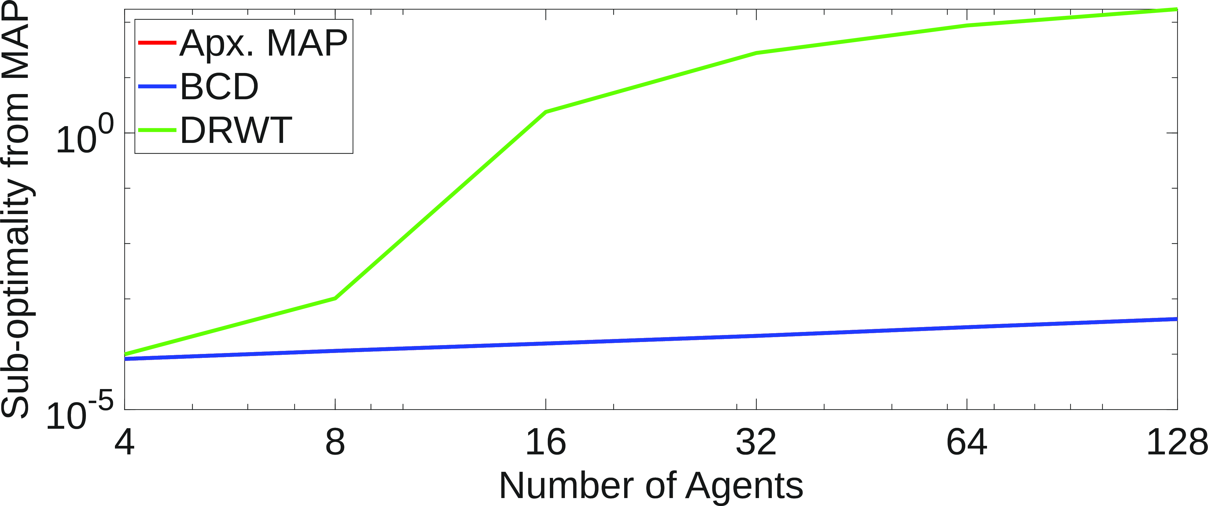
We ran these simulations while varying the number of agents \(N\in\{4, 8, 16, 32, 64, 128\}\), the number of calculations per time step \(k_{\max}\in\{50, 100, 500, 2500, 5000, 10000\}\), and the communication delay \(B\in\{1, 2, 5, 10, 100, 500, 2500, 5000\}\). Additionally, each parameter combination was simulated 8 times with different random number generator initializations1. For each estimate \(\hat{x}\) and MAP estimate \(x\), we compute the sub-optimality from MAP as \(\left\lVert \hat{x} - x \right\rVert_2\).
Figure 2 shows the sub-optimality from MAP for every \(N\in \{4, \ldots, 128\}\) with \(k_{\max}=10000\), \(B=10\), and averaged over the randomized runs. We note that for all \(N\), the BCD curve visually overlaps with the approximate MAP curve, indicating convergence. Additionally, the BCD estimate and the approximate MAP estimate attain a small sub-optimality for all \(N\). In contrast, while DRWT approaches the MAP estimate with 4 agents, the DRWT estimation error increases quickly as the number of agents increases. BCD attains error up to \(64\)% lower than DRWT, and the RMSE between the MAP and the approximate MAP is upper bounded by \(4.4\cdot 10^{-4}\) across all simulations.
7.2 Experimental Results↩︎
We implemented our algorithm with \(4\) agents to estimate the trajectories of \(4\) robots navigating between waypoints. This demonstration was executed on the Robotarium [23], shown in Figure 3. Agent \(1\) uses GPS measurements of robot \(1\), while agent \(i\) for \(i\in\{2,3,4\}\) measures the relative position between robots \(i\) and \(i-1\), which induces dependencies between the agents, shown as green arrows in Figure 3. The demonstration was repeatedly executed for values of \(B\in\{25,50,500,1000,2000,2500,5000\}\) with agents performing \(30000\) onboard calculations per time step. For each \(B\), the agents performed BCD over time steps \(t\in\{1,\dots,20\}\) and advanced time steps after \(1.32\) seconds.

Figure 4 shows the error between the approximate MAP estimate \(x\) and the BCD estimate \(\hat{x}\) over time, computed as \(\left\lVert \hat{x}-x \right\rVert_2\). When \(t\) advances and the problem reinitializes, the error spikes, followed by an exponential decrease as BCD iterations are performed. As shown in Figure 4, the BCD estimates converge to the approximate MAP solution faster for smaller values of \(B\).

8 Conclusion↩︎
We have presented a novel application of block coordinate descent to estimate a sliding window trajectory under partially asynchronous conditions. Compared to synchronous sliding window trajectory estimation, our algorithm attains lower error when performed with lower communication rates. Future work will take advantage of independently selected step sizes for faster convergence.
References↩︎
Code available on GitHub: https://github.com/pooleya19/asynch-dist-estimation-cpp↩︎