CausalMix: Data Mixture as Causal Inference for Language Model Training
July 01, 2026
Abstract
In Large Language Model (LLM) training, data mixing plays a pivotal role in determining model performance. Recent methods optimize mixture weights via proxy models, but they rely on the assumption of static data distributions. As a result, when the
underlying data pool shifts, these methods require costly retraining from scratch. This limitation restricts their ability to scale seamlessly from small settings to larger data pools and model sizes. In this paper, we propose CausalMix to address this limitation by casting data mixture optimization as a causal inference problem. We formulate the statistical features of the data pool as covariates and the domain mixture as the treatment. After fitting a
causal model on 512 runs of Qwen2.5-0.5B to estimate the Conditional Average Treatment Effect (CATE), we extrapolate the optimal mixture for an 800K data pool and apply it to train a 7B model. Furthermore, we successfully generalize the
framework to long chain-of-thought data on Qwen3-4B-Base. By leveraging causal modeling to isolate confounding biases, CausalMix dynamically infers state-dependent optimal data mixtures. Extensive experiments
show that the mixture guided by CausalMix consistently improves performance across multiple downstream tasks, outperforming RegMix and other baselines. In addition, we use the CATE Interpreter to provide visual analysis of
the learned mixing strategy. Overall, CausalMix offers a causal and interpretable framework for optimizing LLM data mixtures.
1 Introduction↩︎
The remarkable capabilities of Large Language Models (LLMs) are driven by the quality and composition of their training data [1]–[4]. During Supervised Fine-Tuning (SFT), where models are aligned with human intent and specialized for complex tasks, the data mixture, namely the relative proportion of different domains such as instruction following, mathematical reasoning, and coding, has a substantial impact on downstream performance [5]. However, determining the optimal mixture remains a notoriously challenging problem. One reason is that training LLMs is expensive, making exhaustive grid search over the continuous simplex of mixture weights intractable for large-scale models.
Existing automated data mixing strategies typically approach this problem through the lens of representation learning or proxy modeling. Methods such as RegMix [6] optimize data weights by minimizing validation loss on a reference dataset, treating historical training runs as independent samples to fit a global mapping from mixture weights to loss. While effective for pre-training, these loss-centric approaches often falter during SFT [7]–[9]. Moreover, global mappings fail to account for the profound impact of the data state, namely the inherent complexity, quality, and difficulty of the specific data pool being used. In other words, a single static optimal mixture does not exist [10], [11].
To bridge this gap, we propose CausalMix, a framework that formulates data mixture optimization not as a black-box hyperparameter search, but as a causal marginal return estimation problem. Instead of seeking a universal mapping from mixture proportions \(T\) to absolute performance \(Y\), we treat historical proxy training runs as treatments. By conditioning on the data state \(X\), characterized by metrics such as normalized loss [12], entropy [13], and writing style [14], we ask a localized causal question: How does a relative change in domain proportions causally affect downstream performance under the current data state?
Drawing upon Double Machine Learning (DML) [15] and causal forests [16], [17], CausalMix orthogonalizes the treatment and outcome variables with respect to the data state. This ensures that the estimated marginal returns are isolated from the confounding effects of the data pool’s inherent quality. Once the causal direction is identified, we employ a conservative policy update, constrained by a trust region, to adjust the mixture weights.
The causal perspective of CausalMix not only provides a principled optimization objective but also unlocks interpretability and transferability. By analyzing the Conditional Treatment Effects (CATE), we empirically unearth the “skill conflicts” between factual knowledge and complex logical reasoning [18], [19], and demonstrate how data quality thresholds dictate the effectiveness of math and coding data. Furthermore, because CausalMix learns the underlying causal dynamics rather than memorizing a specific dataset, it successfully extrapolates to entirely unseen data pools and larger model architectures without requiring new proxy experiments. Taken together, these results position CausalMix as a principled and practical framework for scalable, interpretable, and transferable data mixture optimization in LLM training.
2 Related works↩︎
2.0.0.1 Data mixture optimization.
Data mixture plays an important role in LLM training and strongly affects downstream task performance. Most existing offline methods [6], [20]–[24] focus on the pre-training stage, deriving domain weights through proxy models or modeling training loss as a function of the data mixture. In contrast, data mixture optimization for SFT remains relatively underexplored. Existing SFT-oriented methods, such as DMO [25] and IDEAL [26], still fundamentally use validation loss as the optimization objective. SMART [27] is a relatively rare exception that does not directly optimize validation loss; instead, it formulates data selection as two consecutive cardinality-constrained submodular maximization problems.
2.0.0.2 Causal inference in machine learning.
Integrating causal inference with machine learning helps mitigate spurious correlations and distribution shifts in traditional data-driven models [28], [29]. This line of research is grounded in the potential outcomes framework [30], [31] and causal graphical models [32], [33]. Recent work has mainly progressed along three directions: improving treatment effect estimation through deep representation learning for confounder control [34]–[36] and DML frameworks [15]; uncovering latent data-generating structure through differentiable causal discovery [37] and mechanism disentanglement [38]; and improving generalization by incorporating causal invariance into objectives [39]–[41].
3 Methodology↩︎
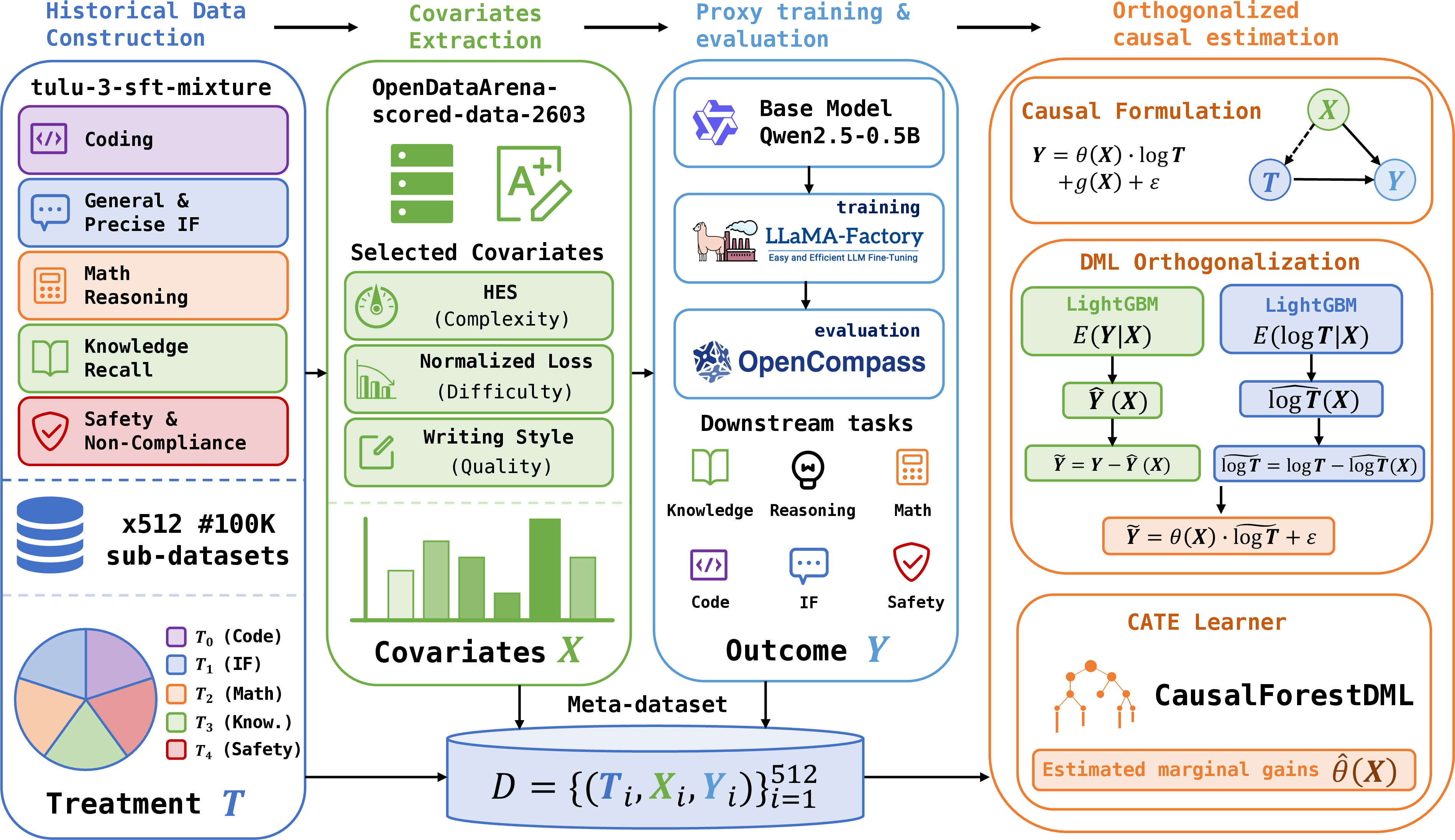
We formulate data mixture optimization as a state-conditioned causal marginal return estimation problem. An overview of the CausalMix pipeline is shown in Figure 1.
3.1 Target estimand and identification↩︎
Given \(K\) data domains and a fixed training budget, a mixture is represented as \[T=(T_1,\ldots,T_K), \qquad T_k\geq 0, \qquad \sum_{k=1}^{K}T_k=1.\] Each training run with a prescribed mixture can be viewed as a data-mixture treatment, and the resulting downstream performance is the corresponding outcome. To simultaneously capture the diminishing marginal returns dictated by empirical scaling laws [7], [42] and accommodate the standard geometric transformations for compositional data on a probability simplex [43], we define the continuous treatment using a log-mixture representation: \[Z=\log(T+\varepsilon),\] where the logarithm is applied element-wise and \(\varepsilon>0\) is a small smoothing constant.
For the \(i\)-th historical proxy run, we observe a triplet \((X_i,T_i,Y_i)\), where covariates \(X_i\) denotes the data state available before training and evaluation, treatment \(T_i\) is the mixture fixed before training, and outcome \(Y_i\) is the downstream performance after training. The state \(X_i\) is a policy context, such as quality, difficulty, complexity, or stylistic statistics of the data pool; it must not include post-training model information or downstream evaluation results. Let \(Y_i(t)\) be the potential outcome that would be obtained if run \(i\) were trained with raw mixture \(t\) under the same training budget, recipe, sampling rule, and evaluation protocol. We define the conditional response function with respect to the corresponding log-mixture \(z=\log(t+\varepsilon)\) as \[\mu(x,z)=\mathbb{E}[Y(t)\mid X=x].\] Learning the full response surface \(\mu(x,z)\) is difficult because the mixture space is continuous and the number of proxy runs is limited. We therefore focus on the local marginal response within the treatment support covered by historical mixtures. For a given \(x\), we use the partially linear approximation [15], [44], [45] \[\mu(x,Z) \approx g(x)+\theta_0(x)^{\top}Z,\] where \(g(x)\) captures the state-dependent baseline performance, and \(\theta_0(x)\in\mathbb{R}^{K}\) is the state-conditioned marginal data return. The quantity \(\theta_0(x)\) can be understood as a generalized CATE for multidimensional continuous treatments. If \(\theta_{0,k}(x)>0\), increasing the relative proportion of domain \(k\) tends to improve downstream performance under state \(x\); if \(\theta_{0,k}(x)<0\), increasing that domain may induce negative transfer. Unlike feature importance in standard supervised learning, \(\theta_0(x)\) describes the local causal response of potential outcomes to mixture treatments.
To identify this quantity from proxy runs, we assume consistency and ignorability by design: \[Y_i=Y_i(T_i), \qquad Y(t)\perp T\mid X.\] The second condition requires that the mixture-generation mechanism be specified before training and evaluation, and that it does not depend on downstream outcomes, training feedback, or other unobserved information that would systematically affect potential outcomes. Since \(Z\) is a deterministic transformation of \(T\), this directly implies \(Y(z)\perp Z\mid X\). We also assume local overlap and local smoothness within the historical treatment support. Under these assumptions, \[\mathbb{E}[Y\mid X=x,Z=z] = \mathbb{E}[Y(z)\mid X=x] = \mu(x,z),\] so the local marginal return \(\theta_0(x)\) is identifiable from proxy mixture experiments. If mixtures are selected adaptively using training or evaluation results, this interpretation should be weakened to a causally motivated marginal-response estimate.
3.2 Orthogonal estimation of marginal returns↩︎
Direct regression is not aligned with our objective, because it mixes state-dependent baseline effects with the causal effect of mixture changes. We address this issue using Double Machine Learning (DML) [15], which residualizes both the outcome and the treatment with respect to the covariates to isolate the local causal response. We therefore define the nuisance functions \[m_0(X)=\mathbb{E}[Y\mid X], \qquad e_0(X)=\mathbb{E}[Z\mid X],\] and construct residuals \[\widetilde{Y}=Y-m_0(X), \qquad \widetilde{Z}=Z-e_0(X).\] The marginal return is estimated from the residualized relation \[\widetilde{Y} \approx \theta_0(X)^{\top}\widetilde{Z}.\] This asks whether deviations in log-mixture proportions beyond their state-conditioned expectation explain performance deviations beyond the state-conditioned baseline.
In practice, the nuisance functions are estimated with cross-fitting [16], [17]: historical proxy runs are split into folds, and each residual is generated by first-stage models trained without the corresponding sample. We then learn a heterogeneous effect model by minimizing the orthogonal loss \[\hat{\theta} = \arg\min_{\theta} \sum_i \left( \widetilde{Y}_i - \theta(X_i)^{\top}\widetilde{Z}_i \right)^2.\] This is an R-loss-style objective: it does not optimize absolute-score prediction, but instead estimates how residual treatment variation explains residual outcome variation.
3.3 From marginal returns to mixture policies↩︎
After estimating the target-state marginal return \(\hat{\theta}(X_{\mathrm{tar}})\) with respect to log-mixture proportions, we convert it into a feasible raw mixture on the simplex. The guiding principle is simple: domains with larger positive log-mixture marginal returns should receive larger weights, while domains with low or negative marginal returns should not be encouraged to increase.
A deterministic analytical extraction maps positive log-mixture marginal returns to the simplex: \[T^{\mathrm{A}}_k = \frac{[\hat{\theta}_k(X_{\mathrm{tar}})]_+}{\sum_{j=1}^{K} [\hat{\theta}_j(X_{\mathrm{tar}})]_+}, \qquad [a]_+=\max(a,0).\] The detailed mathematical proof is provided in Appendix 8. And a search-based extraction instead evaluates a set of raw candidate mixtures \(T^{(1)},\ldots,T^{(M)}\). Each candidate is transformed into its log-treatment representation \(Z^{(m)}=\log(T^{(m)}+\varepsilon)\) before being passed to the fitted causal model. Let \(\widehat{S}(Z^{(m)};X_{\mathrm{tar}})\) denote the predicted score or predicted gain of candidate \(T^{(m)}\) at the target state. The final strategy is obtained by averaging the top candidates in the original mixture space: \[T^{\mathrm{S}} = \frac{1}{K_{\mathrm{top}}} \sum_{m\in\mathrm{Top}} T^{(m)}.\] This can be viewed as local bagging over high-scoring candidates: instead of relying on a single potentially overestimated mixture, it averages several strong raw-mixture candidates to reduce inference noise, smooth the resulting policy, and enhance generalization.
4 Experiments↩︎
In this section, we first describe the experimental setup, then compare CausalMix with strong baselines across different data scales and model sizes, further conduct extension experiments on LongCoT data, and finally present ablation studies. We provide experimental details including introductions of datasets, models, benchmarks and baselines, training and evaluation hyperparameters, and computing costs in Appendix 7.
4.1 Experimental setup↩︎
Data preparation. We use the tulu-3-sft-mixture [46] dataset and adopt the domain partitioning strategy
introduced in Tulu 3. Specifically, we consider five domains: Coding, Instruction Following (IF, combining General and Precise IF), Math Reasoning, Knowledge Recall, and Safety & Non-Compliance. We sample 512 sub-datasets, each containing 100K
instances, and denote the domain mixture proportions of each sub-dataset as the treatment \(T\). To efficiently extract data features, we leverage OpenDataArena-scored-data-2603 [47]–[49], which provides
pre-computed scores on 30 metrics spanning multiple dimensions such as Diversity, Complexity and Quality. A carefully selected subset of these metrics, namely Normalized_Loss [12], Writing_Style [14], and
HES [13], serves as our covariates \(X\). Detailed analysis of this selection is provided in
Section 5.3.
lcccccc>cc>cc Method & Knowledge & Reasoning & Math & Coding & IF & Safety
& \(\mathbf{Avg}_{\mathrm{Dev}}\) & \(\mathbf{Avg}_{\mathrm{Uns}}\)
Qwen2.5-0.5B-Instruct & 29.90 & 32.14 & 35.84 & 34.10 & 30.31 & 11.14 & 28.90 & 28.60
Qwen2.5-7B-Instruct & 60.24 & 52.36 & 54.70 & 68.67 & 44.36 & 60.47 & 56.80 & 46.94
Llama-3.1-Tulu-3-8B-SFT & 51.63 & 67.37 & 56.14 & 57.91 & 68.39 & 46.39 & 57.97 & 41.46
Equal & 27.65 & 29.80 & 23.32 & 33.00 & 33.83 & 14.57 & 27.03 & 24.43
Grid & 28.46 & 31.98 & 30.41 & 33.50 & 20.15 & 23.38 & 27.98 & 23.45
RegMix & 27.29 & 30.04 & 25.53 & 31.28 & 17.01 & 32.56 & 27.28 & 26.24
DoReMi & 29.81 & 31.70 & 22.90 & 33.40 & 35.30 & 25.34 & 29.74 & 24.12
ODM & 27.50 & 30.53 & 25.41 & 33.10 & 26.06 & 23.62 & 27.70 & 23.59
DMO & 28.86 & 30.91 & 22.51 & 30.68 & 35.86 & 26.19 & 29.17 & 26.08
-A & 28.37 & 31.31 & 24.67 & 29.57 & 38.63 & 26.93 & 29.91 & 23.42
-S & 27.27 & 30.23 & 27.77 & 34.94 & 34.94 & 14.81 & 27.85 & 25.90
Equal & 28.39 & 32.98 & 23.96 & 32.10 & 37.89 & 27.78 & 30.51 & 24.71
Grid & 29.34 & 31.84 & 26.68 & 35.02 & 16.64 & 17.26 & 26.13 & 27.08
RegMix & 28.57 & 30.19 & 27.02 & 34.32 & 24.21 & 16.65 & 26.82 & 26.07
DoReMi & 28.58 & 31.12 & 22.14 & 33.61 & 39.74 & 26.56 & 30.29 & 25.69
ODM & 28.65 & 30.74 & 24.35 & 34.62 & 30.50 & 12.61 & 26.91 & 25.51
DMO & 27.74 & 31.75 & 24.25 & 31.80 & 38.63 & 41.62 & 32.63 & 25.84
-A & 28.73 & 30.63 & 24.67 & 30.48 & 42.51 & 43.45 & 33.41 & 24.26
-S & 29.45 & 31.30 & 26.37 & 32.40 & 38.82 & 25.95 & 30.71 & 26.93
Equal & 28.07 & 29.28 & 21.59 & 36.06 & 46.95 & 25.09 & 31.78 & 25.64
Grid & 23.94 & 24.40 & 29.67 & 23.81 & 17.93 & 22.64 & 31.17 & 22.53
RegMix & 24.90 & 29.94 & 30.25 & 25.46 & 25.32 & 22.52 & 26.40 & 22.82
DoReMi & 27.70 & 29.66 & 20.58 & 34.53 & 42.88 & 32.93 & 31.38 & 24.88
ODM & 28.59 & 30.50 & 25.18 & 36.06 & 33.64 & 10.28 & 27.37 & 25.36
DMO & 28.07 & 31.88 & 22.42 & 26.90 & 41.59 & 41.37 & 32.04 & 26.49
-A & 27.93 & 29.68 & 23.56 & 27.76 & 43.81 & 50.92 & 33.94 & 25.02
-S & 28.31 & 30.96 & 27.64 & 30.97 & 42.51 & 36.47 & 32.81 & 25.04
Equal & 60.85 & 64.55 & 59.03 & 53.61 & 68.58 & 53.49 & 60.02 & 49.55
Grid & 59.08 & 68.77 & 65.99 & 61.55 & 44.92 & 56.43 & 59.46 & 46.37
RegMix & 59.60 & 68.12 & 63.37 & 55.76 & 58.04 & 55.94 & 60.14 & 48.12
DoReMi & 58.02 & 63.20 & 57.35 & 57.28 & 68.21 & 52.75 & 59.47 & 46.19
ODM & 60.25 & 65.69 & 59.42 & 44.22 & 63.59 & 54.83 & 58.00 & 48.00
DMO & 59.15 & 63.70 & 60.62 & 54.05 & 70.24 & 54.35 & 60.35 & 48.98
-A & 57.14 & 64.03 & 58.51 & 65.52 & 68.21 & 57.65 & 61.84 & 49.09
-S & 59.35 & 62.88 & 58.63 & 64.43 & 67.47 & 60.95 & 62.28 & 47.98
Proxy model training and evaluation. We select Qwen2.5-0.5B [50], [51] as the proxy
model and conduct training using LlamaFactory [52]. For evaluation, we use OpenCompass [53] to assess the models on a diverse suite of downstream tasks aligned with the training domains, following the Tulu 3 evaluation protocol [46]. We group the downstream tasks into six capabilities: Knowledge, Reasoning, Math, Coding, IF and Safety. We further partition these benchmarks
into Development set \(\mathcal{S}_{\mathrm{Dev}}\) and Unseen set \(\mathcal{S}_{\mathrm{Uns}}\). We adopt the domain-level micro-average score on \(\mathcal{S}_{\mathrm{Dev}}\) as the final outcome \(Y\).
Causal model fitting and inference. We use the EconML [54] framework for causal model fitting and inference. Specifically, we
adopt LightGBM [55] as the first-stage predictor and CausalForestDML [15]–[17] as the core causal estimator;
detailed rationales for these choices are provided in Section 5.1 and Section 5.2. After fitting the causal model on a meta-dataset of 512 historical \((X,T,Y)\) triplets, we set the covariate \(X\) to the comprehensive feature profile of the full tulu-3-sft-mixture training dataset. We consider two variants: CausalMix-A (Analytical), which directly computes the exact closed-form solution. And CausalMix-S (Search), following the practice of RegMix [6], we draw \(100{,}000\) candidate mixtures from a Dirichlet distribution and perform inference on these candidates. We then average the top-100 performing
mixtures to obtain the final strategy.
Baselines. We compare CausalMix against several representative baselines. These include Grid, which denotes the best mixture proportion empirically identified from the 512 proxy-model runs, as well as existing automated mixing methods including RegMix [6], DoReMi [56], ODM [21] and DMO [5]. To ensure a fair comparison, rather than directly adopting the static mixture proportions reported in the original papers, we re-implement these automated methods and train them on our own historical runs following their official protocols. For DMO, we instead use the mixing ratios reported in its paper.
4.2 Main result↩︎
As illustrated in Table ¿tbl:tab:main95result?, CausalMix achieves strong performance on \(\mathbf{Avg}_{\mathrm{Dev}}\) and also demonstrates strong generalization on \(\mathcal{S}_{\mathrm{Uns}}\). Notably, CausalMix-S performs better than CausalMix-A on \(\mathbf{Avg}_{\mathrm{Uns}}\), which may result from averaging the top-100 candidate mixtures: this procedure can smooth out idiosyncratic variance in individual solutions and thus yield a more robust strategy. To reduce the possibility that the observed gains are due to chance, we conduct repeated comparisons across multiple training data scales, ranging from 100K to 800K. Across these settings, our method always outperforms several baselines, especially the recent SFT-oriented state-of-the-art (SOTA) method DMO. Inspired by the rank invariance hypothesis proposed by RegMix [6], we further scale the model size to 7B under the 800K data setting and observe a similar performance trend. This cross-scale consistency further supports the effectiveness and robustness of our approach.
4.3 Extension experiments↩︎
lcc>cccc>cc>cc Method & GSM8K & MATH & \(\mathbf{Avg}_{\mathrm{Math}}\) & HumanEval &
MBPP & \(\mathbf{Avg}_{\mathrm{Code}}\) & \(\mathbf{Avg}\)
Equal & 90.45 & 56.78 & 73.62 & 59.76 & 48.20 & 53.98 & 63.80
Grid & 87.34 & 61.20 & 74.27 & 62.80 & 47.60 & 55.20 & 64.74
RegMix & 89.61 & 40.80 & 65.21 & 61.59 & 53.60 & 57.60 & 61.40
DoReMi & 88.55 & 42.22 & 65.39 & 63.41 & 53.80 & 58.61 & 62.00
ODM & 88.32 & 41.16 & 64.74 & 63.41 & 42.20 & 52.81 & 58.77
DMO & 89.61 & 54.38 & 72.00 & 54.88 & 55.00 & 54.94 & 63.47
& 88.86 & 60.58 & 74.72 & 62.20 & 55.00 & 58.60 & 66.66
To rigorously evaluate the transferability of CausalMix, we conduct an extended generalization experiment across disparate data pools and model architectures. Specifically, we repurpose the historical data from
tulu-3-sft-mixture [46], retain the same covariate selection for \(X\), and define the outcome
\(Y\) as the average downstream performance in the coding and math domains. Subsequently, we apply the trained causal predictor to the entirely unseen dataset AM-Thinking-v1-Distilled-math&code [57] to infer the optimal mixture proportions. To validate the effectiveness of these extrapolated
weights, we train and evaluate Qwen3-4B [58], a model series distinct from the proxy model (the Qwen2.5
series [51]). Empirical evaluations demonstrate that CausalMix consistently achieves the best performance. This robust
transferability demonstrates that our CausalMix successfully captures the intrinsic laws of data mixing, enabling seamless extrapolation across datasets and models without costly proxy-model retraining, and further validating
its effectiveness on LongCoT data.
4.4 Ablation study↩︎
lcccccc>cc Method & Knowledge & Reasoning & Math & Coding & IF & Safety & \(\mathbf{Avg}\)
w/o \(X\) & 29.27 & 31.39 & 29.97 & 33.41 & 39.37 & 36.35 & 33.29
w/o Orth. & 27.41 & 31.29 & 24.74 & 31.90 & 41.04 & 37.82 & 32.66
-A & 27.93 & 29.68 & 23.56 & 27.76 & 43.81 & 50.92 & 33.94
-S & 28.31 & 30.96 & 27.64 & 30.97 & 42.51 & 36.47 & 32.81
w/o \(X\) & 60.45 & 63.95 & 61.16 & 55.62 & 69.69 & 56.92 & 61.30
w/o Orth. & 59.50 & 64.66 & 60.45 & 45.82 & 68.76 & 58.75 & 59.65
-A & 57.14 & 64.03 & 58.51 & 65.52 & 68.21 & 57.65 & 61.84
-S & 59.35 & 62.88 & 58.63 & 64.43 & 67.47 & 60.95 & 62.28
We compare CausalMix against two degraded variants, both of which use LightGBM as the underlying regressor, to validate the necessity of its key components. (1) w/o \(X\). We entirely remove the state covariates, yielding a RegMix-like variant [6]. Unlike RegMix, however, its
optimization target is not validation loss but the average performance on downstream tasks. In this setting, the model reduces to learning a global mapping from treatment to outcome, \(\hat{Y} = g(T).\) By attempting to
learn this static mapping without conditioning on the data state, this context-agnostic variant becomes highly vulnerable to distribution shifts, leading to the performance degradation. (2) w/o Orth. We bypass the DML orthogonalization step and
directly concatenate covariates \(X\) and treatment \(T\) to predict the absolute outcome \(\hat{Y}\), i.e., \(\hat{Y} = f(X,
T).\) As shown in Table ¿tbl:tab:ablation?, this direct regression leads to clear performance degradation, even performing worse than directly fitting \(T\), which further highlights the
regularization bias inherent in standard supervised learning.
5 Analysis↩︎
In this section, we analyze the choices of the causal estimator and covariates. We further use the CATE model interpreter to provide interpretable insights into the dynamics of data mixing.
5.1 Causal model selection↩︎
To identify the most suitable causal estimator, we perform model selection using the R-Scorer (R-loss) metric. The R-Scorer provides a principled and approximately unbiased criterion based on[44]’s orthogonalization technique. It enables us to compare different causal estimators by evaluating how well their predicted causal effects \(\hat{\theta}(X)\)
explain variation in the residual outcomes \(\tilde{Y}\) given the residual treatments \(\tilde{T}\). We evaluate a range of causal estimators in the EconML framework that
support multidimensional continuous treatments, and report the results in Table ¿tbl:tab:model95selection? (a). Among them, CausalForestDML achieves the best performance. We attribute this advantage to its non-parametric,
tree-based recursive partitioning architecture. Unlike linear causal models that impose rigid parametric assumptions, CausalForestDML is suited to capturing the complex interactions between the multidimensional covariates and treatment space.
It also naturally accommodates feature saturation and localized heterogeneous effects, making it particularly suitable for the intricate dynamics of data mixing [15]–[17].
0.38
| Model | RScore (\(\uparrow\)) |
|---|---|
| LinearDML | +0.1445 |
| SparseLinearDML | -1.7065 |
| CausalForestDML | +0.1683 |
| CausalForestDML_Deep | -0.1238 |
| CausalForestDML_Shallow | +0.0207 |
| DML_Poly2_Lasso | +0.1404 |
| DML_Poly2_Ridge | +0.0340 |
| DML_Poly3_Lasso | +0.1533 |
| DML_Poly3_Ridge | +0.0653 |
0.61
| Rank | \(\mathbf{Y}\) Predictor | \(\mathbf{T}\) Predictor | RScore (\(\uparrow\)) | Time (s) |
|---|---|---|---|---|
| 1 | LightGBM | LightGBM | 0.1683 | 12.9 |
| 5 | RandomForest | LightGBM | -0.0556 | 10.3 |
| 6 | RidgeCV | LightGBM | -0.1408 | 6.8 |
| 7 | ElasticNetCV | LightGBM | -0.1681 | 5.5 |
| 8 | GradientBoosting | LightGBM | -0.1686 | 15.4 |
| 19 | RandomForest | RandomForest | -0.2840 | 18.7 |
| 23 | GradientBoosting | RandomForest | -0.3241 | 22.5 |
| 24 | LassoCV | LightGBM | -0.4098 | 11.1 |
| 25 | LightGBM | RandomForest | -0.4323 | 18.0 |
| 29 | GradientBoosting | GradientBoosting | -0.4816 | 10.0 |
5.2 First-stage predictor selection↩︎
The first-stage predictors estimate the conditional expectations \(\hat{Y}(X)\) and \(\hat{T}(X)\). We evaluate a diverse set of regression algorithms and their combinations for the
outcome and treatment models. As summarized in Table ¿tbl:tab:model95selection? (b), with the full results provided in the Appendix, using LightGBM for both models achieves the highest RScore. This configuration substantially
outperforms all other standalone regressors as well as linear models. Notably, LightGBM also emerges as the best treatment predictor across all top-ranked configurations. We attribute this strong performance to LightGBM’s
efficient framework, which handles the multidimensional statistical features while capturing variable interactions without severe overfitting [55]. Although its computational cost is not the lowest among the candidates, this trade-off is acceptable given the substantial performance gains.
5.3 Covariates selection↩︎
In causal inference, covariate selection is of central importance. To efficiently identify the most informative covariates from [49], we randomly sample 64 instances from our 512 historical records as a validation set. Keeping all other hyperparameters fixed, we train distinct causal models with different covariate combinations. We then generate predictions and evaluate them by computing the Spearman rank correlation with the ground-truth scores. We experiment with the vast majority of combinations across different sizes.
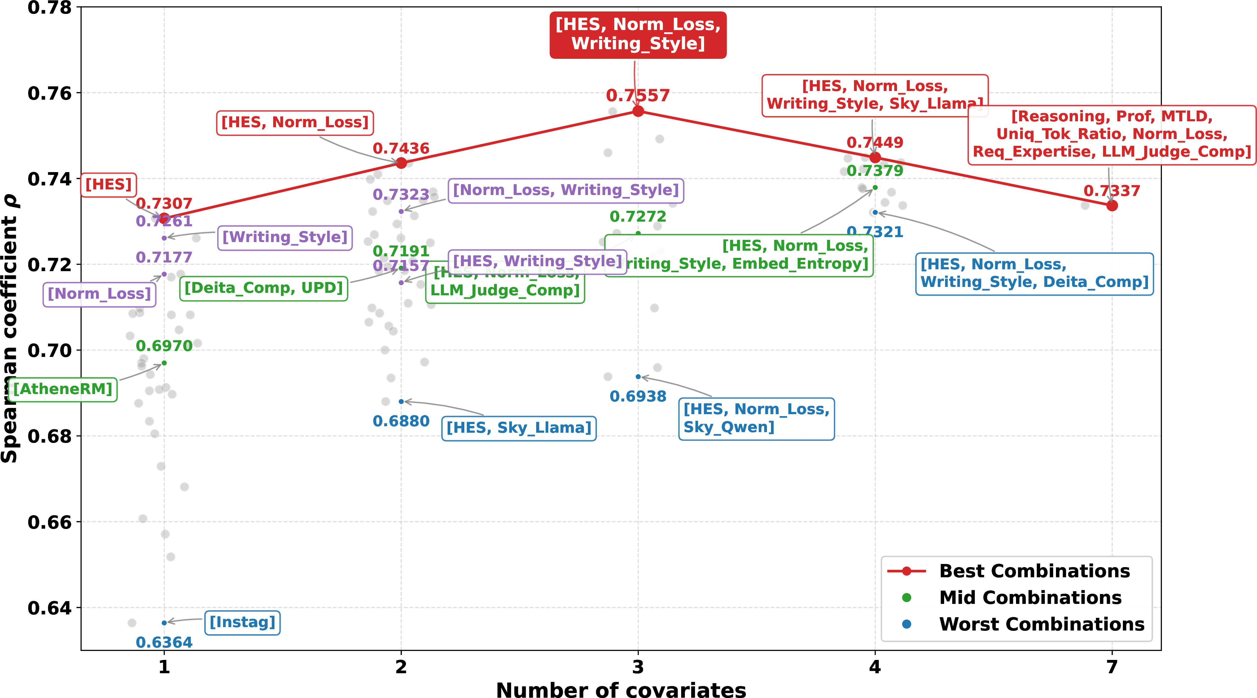
As shown in Figure 2, the best performance is achieved with a combination of three covariates. Specifically, HES sums the entropy of the top 0.5% highest-entropy tokens in reasoning traces produced by
Qwen3-8B to capture critical decision points and genuine reasoning complexity [13]. Normalized_Loss computes the
normalized cross-entropy using Qwen3-8B [12], reflecting data predictability and training utility. Finally,
Writing_Style evaluates the clarity, coherence, and stylistic quality of the text using QuRater-1.3B [14].
These three metrics naturally correspond to the broader dimensions of data Complexity, Difficulty, and Quality, respectively. This leads to an important finding: effective causal modeling requires controlling for a diverse feature profile rather than focusing on only one aspect of the data. However, incorporating too many covariates degrades performance. We attribute this decline primarily to the limited size of our historical meta-dataset, which makes the causal estimator more vulnerable to the curse of dimensionality. For a fair comparison with prior methods such as RegMix [6], we fix the number of proxy models to 512. We expect that scaling up the number of proxy models to support more covariates could further improve performance.
5.4 CATE Interpreter↩︎
We conduct a Tree Interpreter analysis of the trained causal model, as shown in Figure 3. The results show that IF data is the primary driver of downstream alignment, yielding stable positive returns across feature
subspaces. In contrast, Knowledge data has negative effects on difficult target data characterized by high Normalized_Loss and high HES, corroborating the existence of “skill conflicts” between logical reasoning and factual
knowledge injection [18], [19]. Moreover, the marginal returns
of different domains depend strongly on the characteristics of the target data. In low-quality regions, characterized by low Writing_Style and low HES, complex domains such as Math, Coding, and Safety introduce distributional
noise and degrade performance. However, when Writing_Style and HES is moderate, these domains produce strong synergistic gains, effectively mitigating the performance penalty typically associated with Safety data.

6 Conclusion↩︎
In this work, we introduced CausalMix, a framework that shifts SFT data mixture optimization from static validation-loss minimization to state-conditioned causal marginal return estimation. By treating historical proxy training runs as causal treatments and combining orthogonalized estimation with a conservative trust-region policy, CausalMix isolates the marginal utility of domain proportions from the confounding effects of the underlying data state. Extensive experiments show that our approach consistently outperforms strong baselines across different model scales and data budgets, while also exhibiting strong transferability to unseen LongCoT data pools. Furthermore, the interpretable insights derived from our causal framework, including quantified skill conflicts between factual knowledge injection and complex logical reasoning, provide a principled foundation for future research on understanding and optimizing the dynamics of LLM training.
7 Experimental details↩︎
7.1 Datasets↩︎
We evaluate CausalMix on two SFT datasets.
tulu-3-sft-mixture [46] is used to train the Tulu 3 series of models. It contains 939,344 samples spanning
seven domains: General (Tulu 3 Hardcoded, OpenAssistant Guanaco [59], No Robots [60], and WildChat GPT-4 [61], [62]), Knowledge Recall (FLAN v2 [63], SciRIFF [64], and TableGPT [65]), Math Reasoning (Tulu 3 Persona MATH, Tulu 3 Persona GSM, Tulu 3 Persona Algebra, OpenMathInstruct 2 [66], and NuminaMath-TIR [67]), Coding (Tulu 3 Persona Python and Evol CodeAlpaca [68]), Safety &
Non-Compliance (CoCoNot [69], Tulu 3 WildJailbreak [70], and Tulu 3 WildGuardMix [71]), Multilingual
(Aya [72]), and Precise IF (Tulu 3 Persona IF). We exclude the multilingual subset in our experiments.
AM-Thinking-v1-Distilled [57] is a reasoning dataset
distilled from AM-Thinking-v1 [73]. It contains high-quality,
automatically verified responses generated from a shared set of 1.89 million queries spanning a wide range of reasoning domains. Its format and verification pipeline allow for direct comparison and seamless integration into downstream tasks. It is intended
to support the development of open-source language models with strong reasoning abilities. In our experiments, we use the code and math subsets.
We obtain the data-state covariates from OpenDataArena-scored-data-2603 [47]–[49].
OpenDataArena-scored-data-2603 [47]–[49] is a scored SFT dataset collection comprising 63 high-quality instruction-following datasets with nearly 25 million samples. Its core value lies in its 30-dimensional scoring
scheme: each sample is evaluated on metrics such as Normalized_Loss [12], Writing_Style [14], HES [13], and 27 others, enabling fine-grained data selection for filtering, curriculum learning, and mixture optimization.
7.2 Models↩︎
We use Qwen2.5-0.5B as the proxy model, scale the learned mixture strategy up to Qwen2.5-7B, and further conduct an extension experiment on Qwen3-4B-Base.
Qwen2.5 [50] is a series of large language models developed by Qwen. It includes both base and instruction-tuned models
ranging from 0.5B to 72B parameters. Compared with Qwen2 [51], Qwen2.5 offers substantially more knowledge and stronger coding and
mathematical reasoning capabilities, partly due to specialized expert models in these domains. It also improves instruction following, long-form generation (over 8K tokens), structured-data understanding (e.g., tables), and structured output generation,
especially in JSON format. In addition, it is more robust to diverse system prompts, which improves role-play and controllability in chatbot settings. Qwen2.5 supports contexts of up to 128K tokens and can generate up to 8K tokens, and it
supports more than 29 languages, including Chinese, English, French, Spanish, Portuguese, German, Italian, Russian, Japanese, Korean, Vietnamese, Thai, and Arabic. In our experiments, we use the smallest model, Qwen2.5-0.5B, as the proxy and
scale to the widely used Qwen2.5-7B.
Qwen3 [58] is a newer generation of large language models than Qwen2.5 in the Qwen
series, offering a comprehensive suite of dense and mixture-of-experts (MoE) models. Built on extensive pretraining, Qwen3 provides substantial advances in reasoning, instruction following, agent capabilities, and multilingual support. Its key
features include seamless switching between a thinking mode for complex reasoning, mathematics, and coding and a non-thinking mode for efficient general-purpose dialogue within a single model, enabling strong performance across a wide range of scenarios.
It also substantially improves reasoning performance, surpassing previous QwQ [74] models in thinking mode and Qwen2.5-Instruct models in
non-thinking mode on mathematics, code generation, and commonsense reasoning. In addition, Qwen3 shows stronger human preference alignment, with better performance in creative writing, role-playing, multi-turn dialogue, and instruction
following, resulting in a more natural and engaging conversational experience. It also offers strong agent capabilities, enabling effective integration with external tools in both thinking and non-thinking modes and achieving leading performance among
open-source models on complex agentic tasks. Finally, it supports more than 100 languages and dialects and demonstrates strong multilingual instruction-following and translation capabilities. In our extension experiments, we use the 4B dense model.
7.3 Benchmarks↩︎
Following Tulu 3, we assess model performance on multiple tasks and corresponding benchmarks, including Knowledge (MMLU [75], MMLU-Pro [76], GPQA [77]), Reasoning (BBH [78], DROP [79], AGIEval [80]), Math (GSM8K [81], MATH [82], OlympiadBench [83]), Code (HumanEval [84], HumanEval+ [85], MBPP [86]), Instruction Following (IFEval [87], IFBench [88]), and Safety (ToxiGen [89], TruthfulQA [90]).
MMLU [75] is heterogeneous with respect to the reasoning skills required to answer the questions, including instances that require basic factual recall as well as those that demand logical reasoning and problem-solving skills. Following Tulu 3, we use a zero-shot chain-of-thought (CoT) setting that asks the model to “summarize” its reasoning before answering the question. We compute the macro average over all subjects in MMLU as the final task metric.
MMLU-Pro [76] is a 10-way multiple-choice extension of the MMLU dataset. We use essentially the same prompt and answer extraction procedure as in our AGIEval setup, adjusting only the number of answer choices.
GPQA [77] is a set of very challenging multiple-choice questions written by domain experts in biology, physics, and chemistry. We use the same zero-shot prompt and answer extraction procedure as for AGIEval.
BBH (BigBench-Hard) [78] contains challenging reasoning problems for which models benefit from step-by-step reasoning. We use the default setting of OpenCompass [53].
DROP [79] is a reading comprehension task that requires discrete reasoning. We use the default setting of OpenCompass.
AGIEval (English subset) [80] includes the English-language subset of the AGIEval benchmark, specifically
the following multiple-choice tasks: aqua-rat, logiqa-en, lsat-ar, lsat-lr, lsat-rc, sat-en, sat-math, and gaokao-english. We formulate the task using a simple zero-shot CoT prompt
that encourages concise reasoning ending with a clearly stated answer choice. The model’s answer choice is extracted by first matching the requested format, with fallback patterns if the format is not followed precisely. Specifically, we first look for the
exact phrase indicated in the prompt (“Therefore, the answer is [ANSWER]”) and take the last such match. If that fails, we look for a sequence of softer variants, such as “answer is [ANSWER]” or “answer: [ANSWER]”,
before falling back to the last parenthesized letter found; if that also fails, we use the last stand-alone capital letter.
GSM8K [81] contains grade-school math word problems. We use the default setting of OpenCompass.
MATH [82] contains problems from mathematics competitions spanning various categories, such as algebra and calculus. We use the default setting of OpenCompass. We compute the macro average across subsections to obtain the final task metric.
OlympiadBench [83] is an Olympiad-level bilingual multimodal scientific benchmark featuring 8,476 problems from Olympiad-level mathematics and physics competitions, including the Chinese college entrance exam. We evaluate only the English math subset and use the same evaluation logic as for MATH.
HumanEval [84] and HumanEval+ [85] evaluate models’ ability to complete Python code from docstrings. HumanEval+ uses a more rigorous evaluation procedure than the original HumanEval benchmark, with additional tests. We use the default setting of OpenCompass.
MBPP [86] contains 974 programming tasks designed to be solvable by entry-level programmers. We use the default setting of OpenCompass.
IFEval [87] evaluates the instruction-following ability of models in a setting where each instruction corresponds to constraints such that it can be programmatically verified whether the outputs satisfy those constraints. We use the default setting of OpenCompass and measure prompt-level accuracy in the loose evaluation setting.
IFBench [88] is designed to evaluate generalization in precise instruction following on 58 new, diverse, and challenging verifiable out-of-domain constraints. We use the default setting of OpenCompass.
ToxiGen [89] is a large-scale machine-generated dataset of 274k toxic and benign statements about 13 minority groups. We use a zero-shot setting with unnormalized accuracy.
TruthfulQA [90] is a benchmark for measuring whether a language model generates truthful answers to
questions. The benchmark comprises 817 questions spanning 38 categories, including health, law, finance, and politics. We use the test split of mc1 in a zero-shot setting.
We further partition these benchmarks into the development set \(\mathcal{S}_{\mathrm{Dev}}\) and the unseen set \(\mathcal{S}_{\mathrm{Uns}}\). \(\mathcal{S}_{\mathrm{Dev}}\) comprises MMLU, MMLU-Pro, BBH, DROP, GSM8K, MATH, HumanEval, MBPP, IFEval, and TruthfulQA, while \(\mathcal{S}_{\mathrm{Uns}}\) consists of GPQA, AGIEval, OlympiadBench, HumanEval+, IFBench, and ToxiGen.
7.4 Baselines↩︎
We compare CausalMix with recent methods for offline data mixture optimization.
RegMix [6] is designed to automatically identify a high-performing data mixture by formulating the problem as a regression task. It trains many small models on diverse data mixtures, uses regression to predict the performance of unseen mixtures, and applies the best predicted mixture to train a large-scale model with orders of magnitude more compute.
DoReMi [56] first trains a small proxy model using group distributionally robust optimization (Group DRO) over domains to obtain domain weights (mixture proportions) without access to downstream tasks. It then resamples the dataset according to these domain weights and trains a larger full-sized model.
ODM [21] combines elements of both data selection and data mixing. Based on multi-armed bandit algorithms, ODM optimizes the data mixing proportions during training.
DMO [5] frames data mixing as an optimization problem and introduces a method designed to minimize validation loss. DMO parameterizes the loss by modeling effective data transfer and leveraging scaling laws for fine-tuning.
7.5 Computing costs↩︎
We train 512 proxy models with 0.5B parameters, each on 100K SFT examples. The average sequence length is approximately 4096 tokens, and the total estimated FLOPs are \(5.53 \times 10^{20}\). Because our method is state-aware, it maintains strong generalization when transferred to out-of-distribution (OOD) data, as demonstrated by the extension experiments in Section 4.3, without requiring the proxy models to be retrained.
For fair comparison, we use the same proxy-model configuration for baseline methods that require proxy training. Specifically, for RegMix [6], we also use 512 proxy models. For DoReMi [56], we use a single proxy model. For ODM [21], we use a single model to determine the data mixing proportions and training order. For DMO [5], since it is trained on the same data, we directly use the mixture proportions reported in the original paper.
7.6 Hyperparameters↩︎
All random seeds in our experiments are set to 42, and all experiments are conducted on NVIDIA H800 GPUs.
7.6.0.1 Training.
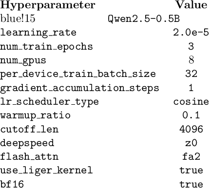
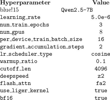
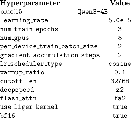
For Qwen2.5-0.5B and Qwen2.5-7B, we follow DMO [5]; for Qwen3-4B-Base, we follow
OpenDataArena [48]. All training hyperparameters are listed in Table ¿tbl:tab:hyper95train?.
7.6.0.2 Evaluation.
All evaluation hyperparameters are listed in Table 1. For Qwen2.5-0.5B and Qwen2.5-7B, we set max_tokens to 4096, whereas for Qwen3-4B-Base, we set it to 32,768. This
difference is determined by whether the training data includes LongCoT-style reasoning.
| Hyperparameter | Value |
|---|---|
| pass@n | n=1 |
| presence_penalty | 0.0 |
| frequency_penalty | 0.0 |
| repetition_penalty | 1.0 |
| temperature | 0.0 |
| top_p | 1.0 |
| top_k | -1 |
| min_p | 0.0 |
| max_tokens | 4096 / 32768 |
| min_tokens | 0 |
8 Proof of the analytical mixture policy↩︎
In this section, we provide a rigorous mathematical derivation for the analytical policy extraction CausalMix-A described in Section 3.3.
Given the estimated state-conditioned marginal return \(\hat{\theta}(X_{\mathrm{tar}}) \in \mathbb{R}^K\), our objective is to find the optimal raw mixture strategy \(T^*\) that maximizes the expected causal performance gain under the Level-Log formulation. This yields a constrained optimization problem over the probability simplex: \[\max_{T} \quad \mathcal{J}(T) = \sum_{k=1}^{K} \hat{\theta}_k \log(T_k)\] \[\text{subject to} \quad \sum_{k=1}^{K} T_k = 1, \quad T_k \geq 0 \quad \forall k \in \{1, \dots, K\}.\]
To explicitly handle the non-negativity constraints, we reformulate the problem as a minimization problem and apply the Karush–Kuhn–Tucker (KKT) conditions. We minimize \(-\mathcal{J}(T)\) and define the Lagrangian \(\mathcal{L}(T, \lambda, \mu)\): \[\mathcal{L}(T, \lambda, \mu) = - \sum_{k=1}^{K} \hat{\theta}_k \log(T_k) + \lambda \left( \sum_{k=1}^{K} T_k - 1 \right) - \sum_{k=1}^{K} \mu_k T_k,\] where \(\lambda \in \mathbb{R}\) is the Lagrange multiplier for the equality constraint, and \(\mu_k \geq 0\) are the KKT multipliers for the inequality constraints \(T_k \geq 0\).
The KKT optimality conditions require that the optimal solution \((T^*, \lambda^*, \mu^*)\) satisfy: (1) Stationarity: \(\frac{\partial \mathcal{L}}{\partial T_k} = -\frac{\hat{\theta}_k}{T_k^*} + \lambda^* - \mu_k^* = 0\), which implies \(\lambda^* - \mu_k^* = \frac{\hat{\theta}_k}{T_k^*}\). (2) Primal feasibility: \(\sum_{k=1}^{K} T_k^* = 1\) and \(T_k^* \geq 0\). (3) Dual feasibility: \(\mu_k^* \geq 0\). (4) Complementary slackness: \(\mu_k^* T_k^* = 0\).
We analyze the optimal solution by partitioning the domains based on the sign of their estimated marginal returns \(\hat{\theta}_k\):
8.0.0.1 Domains with negative or zero marginal returns (\(\hat{\theta}_k \leq 0\)).
Suppose, for the sake of contradiction, that \(T_k^* > 0\). By the complementary slackness condition, \(T_k^* > 0 \implies \mu_k^* = 0\). Substituting this into the stationarity condition yields \(\lambda^* = \frac{\hat{\theta}_k}{T_k^*}\). Since \(\hat{\theta}_k \leq 0\) and \(T_k^* > 0\), this implies \(\lambda^* \leq 0\). However, there must exist at least one domain \(j\) with \(\hat{\theta}_j > 0\) and \(T_j^* > 0\) (otherwise the objective is unbounded negatively, and empirical mixtures always contain positive-return domains). For that domain \(j\), \(\mu_j^* = 0\) implies \(\lambda^* = \frac{\hat{\theta}_j}{T_j^*} > 0\), leading to a contradiction. Furthermore, since \(\log(T_k) \to -\infty\) as \(T_k \to 0\), a negative \(\hat{\theta}_k\) pushes the objective value to \(+\infty\) as \(T_k \to 0^+\). Therefore, the optimal allocation strictly binds at the boundary: \[T_k^* = 0 \quad \text{for all} \quad \hat{\theta}_k \leq 0.\]
8.0.0.2 Domains with positive marginal returns (\(\hat{\theta}_k > 0\)).
Let \(\mathcal{P} = \{k \mid \hat{\theta}_k > 0\}\) denote the active set. For \(k \in \mathcal{P}\), since \(T_k^* > 0\) (otherwise the objective drops to \(-\infty\)), the complementary slackness condition dictates \(\mu_k^* = 0\). The stationarity condition simplifies to: \[\lambda^* = \frac{\hat{\theta}_k}{T_k^*} \implies T_k^* = \frac{\hat{\theta}_k}{\lambda^*}.\] To determine \(\lambda^*\), we invoke the primal feasibility condition over the active set \(\mathcal{P}\): \[\sum_{k \in \mathcal{P}} T_k^* = \sum_{k \in \mathcal{P}} \frac{\hat{\theta}_k}{\lambda^*} = 1 \implies \lambda^* = \sum_{k \in \mathcal{P}} \hat{\theta}_k.\] Substituting \(\lambda^*\) back, we obtain the exact proportional assignment: \[T_k^* = \frac{\hat{\theta}_k}{\sum_{j \in \mathcal{P}} \hat{\theta}_j} \quad \text{for} \quad k \in \mathcal{P}.\]
By unifying both cases, the global optimal solution maps strictly to zero for non-positive causal effects, and scales proportionally for positive effects. This is analytically identical to applying a Rectified Linear Unit (ReLU) activation to the causal marginal returns followed by \(L_1\) normalization: \[T_k^{\mathrm{A}} = \frac{[\hat{\theta}_k(X_{\mathrm{tar}})]_+}{\sum_{j=1}^{K} [\hat{\theta}_j(X_{\mathrm{tar}})]_+}, \qquad \text{where} \quad [a]_+ = \max(a, 0).\] This completes the proof, confirming that our analytical extraction is the mathematically exact closed-form policy under the simplex constraint.