Staleness–Learning Rate Scaling Laws for Asynchronous RLHF
January 01, 1970
Abstract
High-throughput RLHF systems often decouple rollout generation from policy optimization, causing the learner to update on stale rollouts. We study this effect in asynchronous GRPO. The analysis makes the behavior policy explicit in the GRPO surrogate and distinguishes the surrogate-gradient mapping used by the learner from the total derivative of a distribution-dependent population objective. Under local boundedness, distributional smoothness, and behavior-policy smoothness assumptions, stale rollouts induce a per-step surrogate-gradient bias of order \(O(S\eta)\), where \(S\) is the maximum rollout lag and \(\eta\) is the learning rate. We further formulate a conditional collapse-time scaling: when within-cycle drift remains below a batch-level clipping radius, the observed collapse horizon is governed primarily by cumulative learner drift \(T\eta\); when the local stale-rollout condition is binding, stability instead depends explicitly on \(S\eta\). This yields the two-constraint rule \(\eta \ll \min\{R_{\mathrm{batch}}/(S G_{\mathrm{upd}}), R_{\mathrm{crit}}/(T G_{\mathrm{upd}})\}\), explaining why the maximum stable learning rate can appear weakly dependent on staleness only in the horizon-limited regime.
1 Introduction↩︎
Reinforcement Learning from Human Feedback (RLHF) has emerged as a pivotal technique for aligning Large Language Models (LLMs) with human intent, enabling improvements in instruction following, reasoning capabilities, and safety [1]–[3]. The canonical RLHF pipeline, exemplified by InstructGPT [1], typically comprises three stages: supervised fine-tuning (SFT), reward model training on human preference data, and policy optimization via Proximal Policy Optimization (PPO) [4]. Despite its empirical success, this paradigm faces substantial computational challenges: PPO requires maintaining a separate value network (critic) alongside the policy and reward models, creating significant memory overhead and synchronization bottlenecks in distributed training environments [5], [6].
To address these limitations, Group Relative Policy Optimization (GRPO) was introduced by [5] as an efficient alternative to PPO for LLM fine-tuning. GRPO eliminates the critic network by estimating baselines from group-wise reward statistics, reducing memory consumption and computational cost. This design choice has proven effective for mathematical reasoning tasks and has been adopted in subsequent large-scale systems such as DeepSeek-R1 [7]. By removing the critic and lowering the memory and compute cost of each optimization step, GRPO makes distributed asynchronous training increasingly attractive for RLHF pipelines.
Asynchronous training architectures have long been recognized as a promising avenue for accelerating large-scale optimization [8]–[10]. In the standard asynchronous parameter-server framework [11], multiple rollout workers generate experience in parallel using potentially stale policy snapshots, while a central learner continuously applies gradient updates. This decoupling of rollout generation from policy optimization maximizes throughput by reducing idle waiting time. The same idea underlies a long line of decoupled actor-learner architectures in deep RL, beginning with Gorila [12] and A3C [13] and continuing through IMPALA [14], Ape-X [15], and SEED RL [16], where dedicated actors stream experience to a centralized learner. A recurring lesson from this literature is that decoupling is not free: because the actor policy lags the learner, training becomes off-policy, and stable high-throughput learning required explicit corrections—most notably the V-trace off-policy correction introduced by IMPALA [14]. Indeed, some distributed PPO systems deliberately remain synchronous to avoid staleness altogether; DD-PPO [17], for instance, is designed so that “no computation is ever stale,” and reproducibility studies show that even a single step of staleness in actor-learner pipelines measurably alters the learning dynamics [18]. However, the resulting staleness—the discrepancy between the policy used to generate rollouts and the current learner policy—introduces off-policy bias that can destabilize training [10], [19]. Existing convergence analyses of asynchronous SGD typically characterize staleness as a bounded delay [8], [10], yet do not directly quantify how this delay interacts with the distribution shift inherent in policy-gradient methods. Crucially, modern RLHF pipelines based on GRPO [5] typically rely on clipped importance ratios and KL regularization rather than the dedicated off-policy corrections used in classic distributed RL, which makes the staleness–learning-rate interaction the primary lever for controlling stability.
The tension between throughput and stability becomes particularly acute in RLHF because policy-induced distribution shift compounds the staleness effect: as the learner policy evolves, rollouts generated by stale policies become progressively less representative of the current optimization landscape. Empirical observations in asynchronous GRPO suggest a characteristic two-phase pattern—stable improvement followed by abrupt degradation—indicating that the interaction between staleness and learning rate follows structured regimes rather than arbitrary failure. Understanding these regimes is useful for designing asynchronous RLHF systems that exploit parallelism while controlling training instability.
Scaling laws have provided foundational insights into the training dynamics of neural language models [20], [21], characterizing how loss evolves with model size, data volume, and compute budget. More recently, scaling-law formulations have been extended to incorporate learning rate schedules and optimization hyperparameters [22]. However, the interaction between pipeline staleness and learning rate remains less understood, particularly in policy-gradient-based RLHF.
Contributions. This paper develops a local theoretical framework for the staleness–learning rate interaction in asynchronous GRPO training. Our main contributions are:
Behavior-policy-aware formulation. We make the behavior policy explicit in the GRPO surrogate and define a surrogate-gradient mapping \(\mathcal{H}(\theta,\phi)\), separating the learner parameter \(\theta\) from the rollout policy \(\phi\). This avoids identifying the GRPO surrogate gradient with the total derivative of a distribution-dependent objective.
Per-step staleness bias. Under local boundedness, distributional smoothness, and behavior-policy smoothness assumptions, we prove that the stale-rollout surrogate-gradient bias scales as \(O(S\eta)\), yielding a single-step safe region controlled by \(S\eta\).
Conditional collapse-time scaling. We refine the collapse-time argument by distinguishing batch-level clipping from horizon-level learner drift. When the local stale-rollout condition is not binding, collapse follows a \(T\eta\)-type horizon law; otherwise, stability can depend explicitly on \(S\eta\).
Two-constraint stability rule. Combining the two regimes gives a practical condition of the form \(\eta \ll \min\{R_{\mathrm{batch}}/(S G_{\mathrm{upd}}), R_{\mathrm{crit}}/(T G_{\mathrm{upd}})\}\), explaining why the maximum stable learning rate may appear nearly independent of \(S\) only in the horizon-limited regime.
2 Preliminaries↩︎
We study Reinforcement Learning from Human Feedback (RLHF) for Large Language Models (LLMs). Let \(\pi_\theta(\cdot \mid x)\) denote an autoregressive policy parameterized by \(\theta \in \mathbb{R}^d\) that maps a prompt \(x\) to a distribution over completions \(y\). Throughout, \(\theta\) denotes the trainable policy parameters, and all norms and constants are understood in this parameter space.
2.0.0.1 GRPO surrogate objective.
Our analysis focuses on Group Relative Policy Optimization (GRPO) [5], a critic-free RLHF algorithm suited to high-throughput asynchronous pipelines. For each prompt \(x \sim \mathcal{D}\), GRPO samples a group of \(G_{\mathrm{grp}}\) completions \(y_{1:G_{\mathrm{grp}}} \sim \pi_\phi(\cdot \mid x)\) from a behavior policy \(\pi_\phi\), computes per-completion rewards \(r_i = r_{\mathrm{model}}(x,y_i)\), and forms group-normalized advantages \[\hat{A}_i \;=\; \frac{r_i-\mu(r_{1:G_{\mathrm{grp}}})}{\sigma(r_{1:G_{\mathrm{grp}}})}, \qquad i=1,\ldots,G_{\mathrm{grp}}. \label{eq:grpo-advantage}\tag{1}\] For a rollout batch generated by \(\pi_\phi\), define the importance ratio \[\rho_i(\theta,\phi) \;=\; \frac{\pi_\theta(y_i\mid x)}{\pi_\phi(y_i\mid x)} . \label{eq:importance-ratio}\tag{2}\] The behavior-policy-dependent GRPO surrogate, with KL regularization to a reference policy \(\pi_{\mathrm{ref}}\), is \[\ell_{\mathrm{GRPO}}(z;\theta,\phi) \;=\; \frac{1}{G_{\mathrm{grp}}} \sum_{i=1}^{G_{\mathrm{grp}}} \Big[ \operatorname{clip}\!\left(\rho_i(\theta,\phi),1-\epsilon,1+\epsilon\right)\hat{A}_i - \beta\,\mathop{\mathrm{KL}}\!\left(\pi_\theta(\cdot\mid x)\,\|\,\pi_{\mathrm{ref}}(\cdot\mid x)\right) \Big], \label{eq:grpo-surrogate}\tag{3}\] where \(z=(x,y_{1:G_{\mathrm{grp}}})\) is a group instance. The explicit behavior-policy argument \(\phi\) captures the denominator of the importance ratio, the clipping boundary induced by the rollout policy, and the group statistics of the sampled batch. We reserve \(G_{\mathrm{grp}}\) for the GRPO group size; gradient and update magnitude constants are denoted separately below.
2.0.0.2 Rollout distribution.
Let \(p(\cdot;\phi)\) denote the distribution over group instances induced by sampling \(x\sim\mathcal{D}\) and \(y_{1:G_{\mathrm{grp}}}\sim \pi_\phi(\cdot\mid x)\). Because this distribution depends on the policy used to generate rollouts, the theory below works with the GRPO surrogate-gradient mapping rather than the total derivative of an objective of the form \(\mathbb{E}_{z\sim p(\cdot;\theta)}[\ell(z;\theta)]\).
2.0.0.3 Stochastic gradients under stale rollouts.
In practice, stochastic gradients are computed at learner parameters \(\theta\) using a batch \(\mathcal{B}_\phi\) collected under a possibly different behavior policy \(\pi_\phi\): \[g(\theta;\mathcal{B}_\phi) \;\triangleq\; \frac{1}{|\mathcal{B}_\phi|} \sum_{z\in\mathcal{B}_\phi} \nabla_\theta \ell_{\mathrm{GRPO}}(z;\theta,\phi), \qquad z\sim p(\cdot;\phi). \label{eq:grpo-gradient}\tag{4}\] We use gradient ascent notation throughout, treating \(\ell_{\mathrm{GRPO}}\) as a utility to be maximized. While the notation is specialized to GRPO, the bias decomposition in Section 3 applies to RLHF policy-optimization methods whose stochastic gradient has the behavior-policy-dependent form in 4 .
2.0.0.4 Synchronous vs. asynchronous updates.
Let \(\eta>0\) denote the learning rate.
Synchronous (on-policy) update. Rollouts are generated by the current policy (\(\phi=\theta_t\)), and the learner updates \[\theta_{t+1} \;=\; \theta_t + \eta\,g(\theta_t;\mathcal{B}_{\theta_t}). \label{eq:sync-update}\tag{5}\]
Asynchronous (stale-rollout) update. To maximize throughput, rollout workers may generate trajectories using a stale snapshot \(\theta_{t-k_t}\), where \(k_t\ge 0\) is the staleness lag at step \(t\). The learner updates \[\theta_{t+1} \;=\; \theta_t + \eta\,g(\theta_t;\mathcal{B}_{\theta_{t-k_t}}). \label{eq:async-update}\tag{6}\] We denote the maximum staleness by \(S\triangleq \sup_t k_t\). Throughout this paper, \(S\) is the central pipeline design knob: a larger \(S\) permits higher rollout throughput at the cost of greater off-policy error. Our goal is to quantify the bias introduced by staleness in 6 and derive scaling rules relating \((S,\eta)\) for both a single-step safe region and a finite training horizon.
3 Method: The Staleness-Aware Scaling Law↩︎
Asynchronous SGD analyses typically assume bounded delay, but do not directly characterize how delay interacts with policy-induced distribution shift in RLHF. In this section, we study this interaction in asynchronous GRPO. We first define a behavior-policy-aware surrogate-gradient mapping and use it to bound the per-step staleness bias induced by stale rollouts. This gives a single-step scaling rule controlled by \(S\eta\) (Theorem 1). We then state a conditional collapse-time scaling that applies when the local stale-rollout condition is not the binding failure mode (Theorem 2).
3.1 Assumptions↩︎
Assumption 1 (Local bounded surrogate gradient and update). Within the local training region considered by the analysis, there exist constants \(G_{\mathrm{grad}},G_{\mathrm{upd}}>0\) such that for all relevant learner parameters \(\theta\), behavior policies \(\phi\), and group instances \(z\), \[\bigl\|\nabla_\theta \ell_{\mathrm{GRPO}}(z;\theta,\phi)\bigr\| \le G_{\mathrm{grad}}, \label{eq:bounded-grad}\tag{7}\] and the applied update direction satisfies \[\bigl\|g(\theta;\mathcal{B}_\phi)\bigr\| \le G_{\mathrm{upd}}. \label{eq:bounded-update}\tag{8}\]
The first part controls the magnitude of the per-instance surrogate gradient; the second part controls the actual learner displacement and can be enforced by update or gradient clipping. For plain minibatch ascent, one may take \(G_{\mathrm{upd}}\le G_{\mathrm{grad}}\) under 7 . The boundedness assumption is used as a local condition in the stable training region rather than as a global statement about all language-model parameters.
Assumption 2 (Local distributional smoothness). There exists \(C_\pi>0\) such that for any behavior policies \(\phi,\phi'\) in the local training region, \[\mathop{\mathrm{KL}}\!\left(p(\cdot;\phi)\,\|\,p(\cdot;\phi')\right) \le C_\pi \|\phi-\phi'\|^2, \label{eq:kl-smoothness}\tag{9}\] where \(p(\cdot;\phi)\) denotes the distribution over group instances induced by \(\pi_\phi\).
Assumption 3 (Behavior-policy smoothness of the surrogate). There exists \(L_\rho>0\) such that, for any learner parameter \(\theta\) and behavior policies \(\phi,\phi'\) in the local training region, \[\left\| \mathbb{E}_{z\sim p(\cdot;\phi)} \left[ \nabla_\theta \ell_{\mathrm{GRPO}}(z;\theta,\phi) - \nabla_\theta \ell_{\mathrm{GRPO}}(z;\theta,\phi') \right] \right\| \le L_\rho\|\phi-\phi'\|. \label{eq:behavior-smoothness}\tag{10}\]
Assumption 3 captures the local sensitivity of the importance-ratio denominator, clipping boundary, and group-normalized advantages to the behavior policy. It is not intended as a global smoothness claim; it is the regime in which the stale-rollout analysis is meant to be applied.
Remark 1 (Relevance to GRPO). The KL regularizer in GRPO, either with a fixed coefficient \(\beta\) or through a target-KL controller, keeps successive policies locally close in the stable training regime, supporting the local nature of Assumption 2. All norms and constants are understood in the policy’s trainable-parameter space.
3.1.0.1 Pipeline convention.
We follow the asynchronous-GRPO pipeline in which a rollout batch generated by \(\pi_{\theta_\tau}\) is consumed by the learner for \(S\) consecutive optimization steps before being refreshed. Thus the policy lag \(k_t\) at learner step \(t\) ranges from \(0\) to \(S-1\) within each rollout cycle, and \(S\) is both the maximum staleness and the rollout reuse factor. Consequently, the \(M\)-th rollout batch corresponds approximately to learner steps \(t\in\{(M-1)S,\dots,MS-1\}\), so \[t\approx MS. \label{eq:rollout-to-step}\tag{11}\]
3.2 Staleness as a Controlled Bias↩︎
Let \(\theta_t\) be the learner policy at optimization step \(t\) and let \[\phi_t \triangleq \theta_{t-k_t} \label{eq:phi-t}\tag{12}\] be the behavior policy used to generate the batch consumed at step \(t\). Define the population GRPO surrogate-gradient mapping \[\mathcal{H}(\theta,\phi) \triangleq \mathbb{E}_{z\sim p(\cdot;\phi)} \left[ \nabla_\theta \ell_{\mathrm{GRPO}}(z;\theta,\phi) \right], \label{eq:H-def}\tag{13}\] and the on-policy surrogate-gradient mapping \[\mathcal{H}_{\mathrm{on}}(\theta) \triangleq \mathcal{H}(\theta,\theta). \label{eq:H-on-def}\tag{14}\] These quantities are the gradients actually used by the GRPO surrogate update; they should not be confused with the total derivative of a distribution-dependent objective.
Taking expectation over batch sampling, \[\mathbb{E}\!\left[g(\theta_t;\mathcal{B}_{\phi_t})\right] = \mathcal{H}(\theta_t,\phi_t). \label{eq:expected-async}\tag{15}\] Adding and subtracting the on-policy surrogate gradient gives \[\mathbb{E}\!\left[g(\theta_t;\mathcal{B}_{\phi_t})\right] = \mathcal{H}_{\mathrm{on}}(\theta_t)+\delta_t, \label{eq:decomposition}\tag{16}\] where \[\delta_t \triangleq \mathcal{H}(\theta_t,\phi_t)-\mathcal{H}(\theta_t,\theta_t). \label{eq:delta-def}\tag{17}\] The term \(\delta_t\) is the staleness bias: it captures the systematic difference between optimizing on stale rollout data and optimizing on data sampled from the current policy, including both distribution shift and behavior-policy dependence of the surrogate.
3.3 Bounding the Staleness Bias↩︎
Lemma 1 (Per-step staleness bias). Under Assumptions 1–3, \[\|\delta_t\| \le C_{\mathrm{stale}}\|\theta_t-\phi_t\|, \label{eq:bias-bound}\tag{18}\] where \[C_{\mathrm{stale}} \triangleq L_\rho + 2G_{\mathrm{grad}}\sqrt{C_\pi/2}. \label{eq:cstale-def}\tag{19}\]
Proof. Using \(\phi_t=\theta_{t-k_t}\), decompose \[\begin{align} \delta_t &= \mathbb{E}_{z\sim p(\cdot;\phi_t)} \left[\nabla_\theta \ell_{\mathrm{GRPO}}(z;\theta_t,\phi_t)\right] - \mathbb{E}_{z\sim p(\cdot;\theta_t)} \left[\nabla_\theta \ell_{\mathrm{GRPO}}(z;\theta_t,\theta_t)\right]\\ &= \underbrace{ \mathbb{E}_{z\sim p(\cdot;\phi_t)} \left[ \nabla_\theta \ell_{\mathrm{GRPO}}(z;\theta_t,\phi_t) - \nabla_\theta \ell_{\mathrm{GRPO}}(z;\theta_t,\theta_t) \right] }_{\text{behavior-policy surrogate shift}}\\ &\quad+ \underbrace{ \mathbb{E}_{z\sim p(\cdot;\phi_t)} \left[\nabla_\theta \ell_{\mathrm{GRPO}}(z;\theta_t,\theta_t)\right] - \mathbb{E}_{z\sim p(\cdot;\theta_t)} \left[\nabla_\theta \ell_{\mathrm{GRPO}}(z;\theta_t,\theta_t)\right] }_{\text{rollout distribution shift}}. \end{align}\] The first term is bounded by \(L_\rho\|\theta_t-\phi_t\|\) by Assumption 3. For the second term, let \(h(z)=\nabla_\theta\ell_{\mathrm{GRPO}}(z;\theta_t,\theta_t)\). By Assumption 1, \(\|h(z)\|\le G_{\mathrm{grad}}\). Therefore, for \(P=p(\cdot;\phi_t)\) and \(Q=p(\cdot;\theta_t)\), \[\|\mathbb{E}_P[h(z)]-\mathbb{E}_Q[h(z)]\| \le 2G_{\mathrm{grad}}\,\mathrm{TV}(P,Q).\] Pinsker’s inequality and Assumption 2 give \[\mathrm{TV}\!\left(p(\cdot;\phi_t),p(\cdot;\theta_t)\right) \le \sqrt{\frac{1}{2}\mathop{\mathrm{KL}}\!\left(p(\cdot;\phi_t)\,\|\,p(\cdot;\theta_t)\right)} \le \sqrt{C_\pi/2}\,\|\theta_t-\phi_t\|.\] Combining the two bounds yields 18 . ◻
3.4 Single-Step Staleness Scaling↩︎
We next relate the stale-policy drift \(\|\theta_t-\phi_t\|\) to the learning rate and policy lag. From the asynchronous update rule and Assumption 1, \[\|\theta_t-\phi_t\| = \|\theta_t-\theta_{t-k_t}\| \le \sum_{j=1}^{k_t} \eta\,\bigl\|g(\theta_{t-j};\mathcal{B}_{\theta_{t-j-k_{t-j}}})\bigr\| \le k_t\eta G_{\mathrm{upd}} \le S\eta G_{\mathrm{upd}}. \label{eq:drift}\tag{20}\] Combining Lemma 1 with 20 gives the main single-step scaling law.
Theorem 1 (Single-step staleness scaling). Under Assumptions 1–3, the staleness bias at step \(t\) satisfies \[\|\delta_t\| \le C_{\mathrm{stale}}k_t\eta G_{\mathrm{upd}} \le C_{\mathrm{stale}}S\eta G_{\mathrm{upd}}. \label{eq:linear-scaling}\tag{21}\] Consequently, the asynchronous GRPO update can be written as \[\theta_{t+1} = \theta_t + \eta\left( \mathcal{H}_{\mathrm{on}}(\theta_t)+\xi_t+\delta_t \right), \label{eq:effective-update}\tag{22}\] where \[\xi_t \triangleq g(\theta_t;\mathcal{B}_{\phi_t}) - \mathcal{H}(\theta_t,\phi_t) \label{eq:noise-def}\tag{23}\] is a zero-mean sampling noise term conditional on \((\theta_t,\phi_t)\), and \(\delta_t\) obeys 21 .
3.4.0.1 Single-step implication.
The bias in the gradient estimator scales as \(O(S\eta)\), and the staleness-induced perturbation to a single parameter update scales as \[\eta\|\delta_t\| = O(S\eta^2). \label{eq:single-step-perturbation}\tag{24}\] Keeping the stale-rollout drift small relative to the local trust region gives a single-step safe region of the form \[S\eta \lesssim C_{\mathrm{safe}}, \label{eq:safe-region}\tag{25}\] where \(C_{\mathrm{safe}}\) absorbs the local trust-region radius, target-KL budget, curvature, and effective update scale.
3.5 Collapse-Time Scaling↩︎
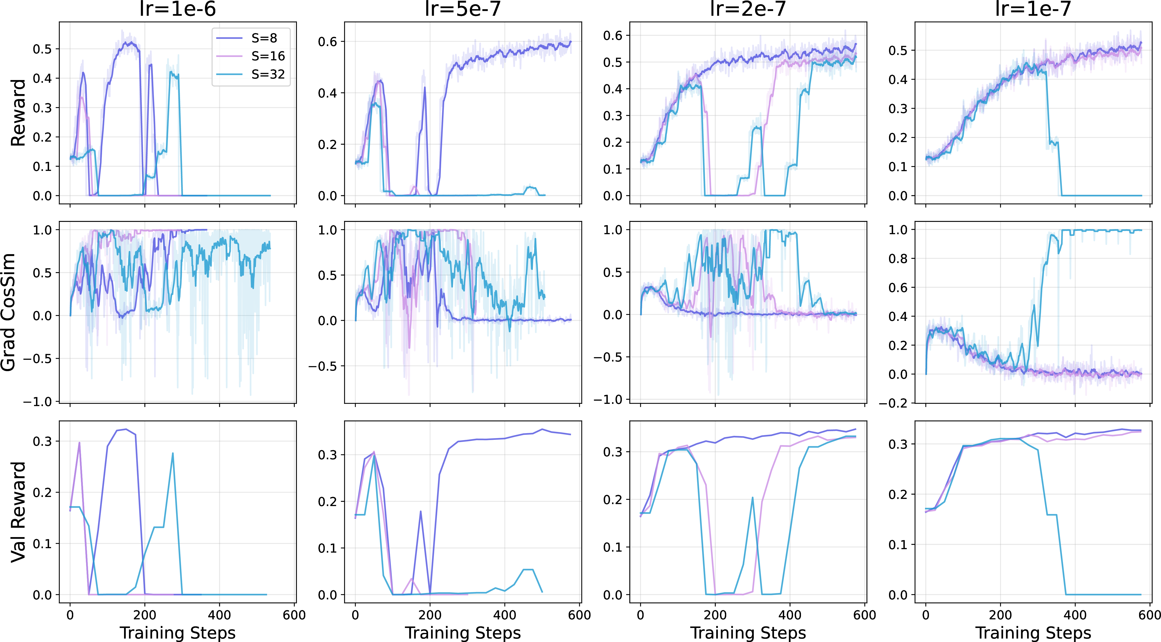
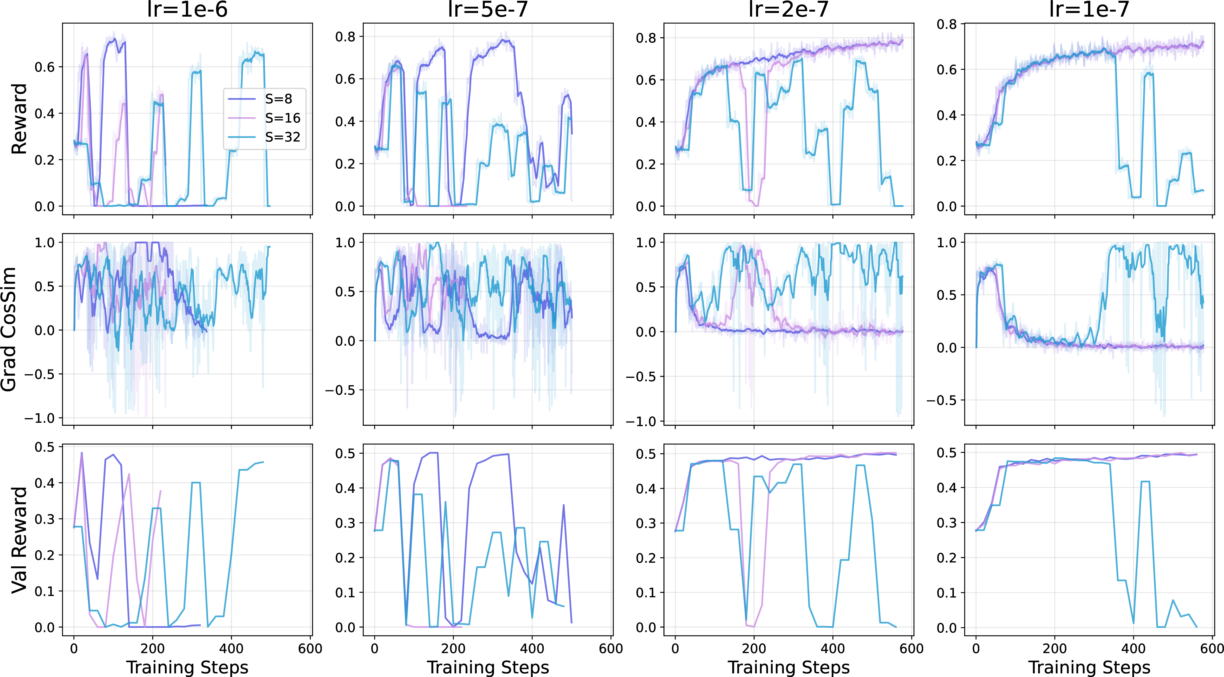
Theorem 1 bounds the per-step bias, but it does not by itself determine when an unstable configuration will fail. Empirically, high-learning-rate configurations can train normally for several rollout batches and then collapse abruptly (Figures 1 and 2). We now separate two mechanisms: batch-level stale-rollout clipping and horizon-level learner drift.
3.5.0.1 Batch-level clipping radius.
Consider a rollout batch generated by \(\pi_\phi\) and consumed under learner policy \(\pi_\theta\). The clipped importance ratio \(\operatorname{clip}(\rho_i(\theta,\phi),1-\epsilon,1+\epsilon)\) provides a meaningful policy-gradient signal only while a sufficient fraction of sampled ratios remain inside, or close to, the clipping interval. Let \(R_{\mathrm{batch}}(\epsilon)\) denote a local radius such that the batch-level clipped-ratio signal remains non-degenerate whenever \[\|\theta-\phi\| \ll R_{\mathrm{batch}}(\epsilon). \label{eq:rbatch-def}\tag{26}\] Within one rollout reuse cycle, Eq. 20 gives \(\|\theta_t-\phi_t\|\le S\eta G_{\mathrm{upd}}\). Thus batch-level stale-rollout clipping is controlled by \(S\eta\), not by the cumulative number of learner steps since initialization.
3.5.0.2 Horizon-level learner drift.
Suppose the local stale-rollout condition \[S\eta G_{\mathrm{upd}} \ll R_{\mathrm{batch}}(\epsilon) \label{eq:local-stale-condition}\tag{27}\] is satisfied, so within-cycle clipping caused by stale rollouts is not the binding failure mode. Training may still collapse when the learner leaves a broader local surrogate-validity region of radius \(R_{\mathrm{crit}}\). This radius summarizes the range over which the GRPO surrogate, local curvature, and reference-policy regularization continue to provide a reliable optimization signal. Under the update bound in Assumption 1, \[\|\theta_t-\theta_0\| \le \sum_{s=0}^{t-1}\eta\,\bigl\|g(\theta_s;\mathcal{B}_{\phi_s})\bigr\| \le t\eta G_{\mathrm{upd}}. \label{eq:total-drift}\tag{28}\] Therefore, reaching a horizon-level radius \(R_{\mathrm{crit}}\) requires \(t\eta G_{\mathrm{upd}}\gtrsim R_{\mathrm{crit}}\).
Theorem 2 (Conditional collapse-time scaling, informal). Assume Assumptions 1–3 and the local stale-rollout condition 27 . If collapse is governed by the learner leaving a surrogate-validity region of radius \(R_{\mathrm{crit}}\), then the first collapse step satisfies \[t_{\mathrm{collapse}}\cdot\eta \gtrsim \frac{R_{\mathrm{crit}}}{G_{\mathrm{upd}}}. \label{eq:t-collapse-bound}\tag{29}\] Equivalently, in rollout-batch units, using \(t_{\mathrm{collapse}}\approx M_{\mathrm{collapse}}S\), \[M_{\mathrm{collapse}}S\eta \gtrsim \frac{R_{\mathrm{crit}}}{G_{\mathrm{upd}}}. \label{eq:m-collapse-bound}\tag{30}\] If \(S\eta G_{\mathrm{upd}}\) is comparable to or larger than \(R_{\mathrm{batch}}(\epsilon)\), collapse can instead be governed by within-cycle stale-rollout clipping, and the learner-step collapse time may depend explicitly on \(S\).
3.5.0.3 When \(S\) does not appear in the learner-step horizon.
Theorem 1 and Theorem 2 describe different quantities. Theorem 1 bounds the direction error of an individual gradient estimator and therefore produces an \(S\eta\) condition. Theorem 2 describes the horizon-level learner displacement after the \(S\eta\) condition is already controlled. In that horizon-limited regime, increasing \(S\) mainly changes how many rollout batches correspond to a fixed number of learner steps: a larger \(S\) packs more learner steps into each rollout batch, so collapse can occur at a smaller batch count \(M_{\mathrm{collapse}}\) even if the learner-step horizon is similar.
3.5.0.4 Two-tier picture.
Combining the two results gives the following interpretation:
Local stale-rollout condition: \(S\eta G_{\mathrm{upd}}\ll R_{\mathrm{batch}}(\epsilon)\) keeps within-cycle stale-rollout bias and clip saturation controlled.
Horizon-level drift condition: \(t\eta G_{\mathrm{upd}}\lesssim R_{\mathrm{crit}}\), equivalently \(MS\eta G_{\mathrm{upd}}\lesssim R_{\mathrm{crit}}\), keeps the cumulative learner drift inside the surrogate-validity region.
The first condition can make the stable learning rate decrease with \(S\); the second can make the observed threshold appear nearly independent of \(S\) when it is the active constraint.
3.6 Practical Stability Rule↩︎
For a target training horizon of \(T\) learner steps, a configuration \((S,\eta)\) should satisfy both a local stale-rollout condition and a horizon-level drift condition: \[S\eta \ll \frac{R_{\mathrm{batch}}(\epsilon)}{G_{\mathrm{upd}}}, \qquad T\eta \ll \frac{R_{\mathrm{crit}}}{G_{\mathrm{upd}}}. \label{eq:two-conditions}\tag{31}\] Equivalently, \[\eta \ll \min\left\{ \frac{R_{\mathrm{batch}}(\epsilon)}{S G_{\mathrm{upd}}}, \frac{R_{\mathrm{crit}}}{T G_{\mathrm{upd}}} \right\}. \label{eq:practical-rule}\tag{32}\] The apparent dependence of the maximum stable learning rate on \(S\) depends on which constraint is active. When the horizon-level condition is binding, \[\frac{R_{\mathrm{crit}}}{T G_{\mathrm{upd}}} \ll \frac{R_{\mathrm{batch}}(\epsilon)}{S G_{\mathrm{upd}}}, \label{eq:horizon-binding}\tag{33}\] the maximum stable learning rate is approximately independent of \(S\), and increasing \(S\) primarily reduces the number of rollout batches before collapse through \(M_{\mathrm{collapse}}S\eta\gtrsim R_{\mathrm{crit}}/G_{\mathrm{upd}}\). When the local stale-rollout condition is binding, however, the stable learning rate decreases as \(1/S\).
3.6.0.1 Scope.
This analysis does not claim that stale rollouts are harmless. It separates two effects: the per-step stale-rollout bias controlled by \(S\eta\), and the horizon-level learner drift controlled by \(T\eta\). The empirical observation that the learning-rate threshold can be weakly dependent on \(S\) should therefore be interpreted as evidence for the horizon-limited regime, not as a general guarantee that staleness never affects stability.
4 Experiments↩︎
Our experiments are designed to test the two-tier picture of Section 3 term by term, rather than merely to demonstrate that staleness can destabilize training. Each of the three result subsections below targets one prediction of the theory and follows the same Prediction \(\rightarrow\) Observation \(\rightarrow\) Takeaway structure, so that every empirical claim is tied to a specific theorem or equation. Table 1 summarizes this correspondence.
| Theoretical prediction | Empirical question | Evidence |
|---|---|---|
| Local stale-rollout condition \(S\eta\lesssim R_{\mathrm{batch}}/G_{\mathrm{upd}}\) (Thm. [thm:scaling], Eq. [eq:safe-region]) | Does the maximum stable learning rate fall as \(\eta_{\max}\!\propto\!1/S\)? | §[sec:subsec:phase], Figs. [fig:metrics95grid951b]–[fig:metrics95grid953b] |
| Horizon-limited collapse \(t_{\mathrm{collapse}}\eta\gtrsim R_{\mathrm{crit}}/G_{\mathrm{upd}}\) (Thm. [thm:collapse], Eqs. [eq:t-collapse-bound]–[eq:m-collapse-bound]) | For collapsing runs, is the collapse horizon set by \(T\eta\) and independent of \(S\)? | §[sec:subsec:escape], Table [tbl:tab:collapse] |
| Update decomposition \(g=\mathcal{H}_{\mathrm{on}}+\xi_t+\delta_t\) with \(\|\delta_t\|=O(S\eta)\) (Thm. [thm:scaling], Eq. [eq:effective-update]) | Do the stable/unstable regimes correspond to diffusive/ballistic drift? | §[sec:subsec:coherence], Fig. [fig:smalllr953b] |
4.1 Datasets, Models, and Evaluation Metrics↩︎
4.1.0.1 Task and reward.
We train on a mathematical-reasoning task with a rule-based, verifiable reward: a completion receives reward \(1\) if its final answer matches the ground truth and \(0\) otherwise. This binary, low-variance signal isolates the optimization dynamics of interest from reward-model noise, so that any collapse can be attributed to the staleness–learning-rate interaction rather than to reward hacking. We hold out a fixed validation split that is never used for rollouts.
4.1.0.2 Models.
We use two instruction-tuned policies of different scale, Llama-3.2-1B-Instruct and Llama-3.2-3B-Instruct, optimized with GRPO [5]. Following the convention of Section 2, all parameter norms, drift quantities, and constants are measured in the policy’s trainable-parameter space. A KL penalty to the SFT
reference policy keeps successive policies locally close, consistent with the local-smoothness regime of Assumptions 2–3.
4.1.0.3 Asynchronous pipeline.
We adopt the rollout-reuse pipeline of Section 3: a rollout batch generated by the snapshot \(\pi_{\theta_\tau}\) is consumed by the learner for \(S\) consecutive optimization steps before the rollout workers refresh their weights. A weight synchronization (or weight sync) thus marks the boundary between consecutive rollout cycles, and the \(M\)-th weight sync occurs at learner step \(t\approx MS\) (Eq. 11 ). We sweep the maximum staleness \(S\in\{8,16,32\}\) against the learning rate \(\eta\in\{1\!\times\!10^{-6},\,5\!\times\!10^{-7},\,2\!\times\!10^{-7},\,1\!\times\!10^{-7}\}\), holding all other hyperparameters (group size, batch size, clip range \(\epsilon\), KL coefficient \(\beta\)) fixed across runs so that \((S,\eta)\) is the only varying factor.
4.1.0.4 Evaluation metrics.
We track three quantities, each chosen to probe a specific term in the theory.
Training Reward: the mean group reward per optimization step. A collapse manifests as the reward dropping to and remaining at zero; this is our operational definition of instability.
Gradient Cosine Similarity (Grad CosSim): the cosine similarity between consecutive applied update directions, \(\cos\!\big(g(\theta_{t};\mathcal{B}_{\phi_{t}}),\,g(\theta_{t-1};\mathcal{B}_{\phi_{t-1}})\big)\). This is our direct probe of which term dominates the update in Eq. 22 : a persistently high value indicates a coherent direction (the staleness bias \(\delta_t\)), whereas a value near zero indicates that the zero-mean sampling noise \(\xi_t\) dominates and successive steps decorrelate.
Validation Reward: the reward on the held-out split, evaluated periodically, used to confirm that a training-reward collapse reflects a genuine loss of the optimization signal rather than a metric artifact.
4.2 Staleness Lowers the Maximum Stable Learning Rate↩︎
4.2.0.1 Theory prediction.
The single-step safe region \(S\eta\lesssim C_{\mathrm{safe}}\) of Eq. 25 , equivalently the first term \(S\eta\ll R_{\mathrm{batch}}/G_{\mathrm{upd}}\) of the two-constraint rule 32 , predicts that the maximum stable learning rate should scale inversely with staleness, \(\eta_{\max}\propto 1/S\), so that the product \(S\,\eta_{\max}\) is approximately constant.
4.2.0.2 Observation.
Figures 1 and 2 sweep \((S,\eta)\) for the 1B and 3B policies. Reading across each row (fixed \(\eta\), increasing \(S\)) and down each column (fixed \(S\), decreasing \(\eta\)) reveals a clear monotone phase structure: the larger the staleness, the smaller the learning rate required to maintain stability. At the largest learning rate \(\eta=10^{-6}\), every staleness setting eventually collapses to zero reward. As \(\eta\) is reduced, the stable region expands from large-\(S\) to small-\(S\) configurations, and at \(\eta=10^{-7}\) the small- and moderate-staleness runs (\(S=8,16\)) converge stably while only \(S=32\) remains unstable. Quantitatively, the stability boundary \(\eta_{\max}(S)\) moves down by roughly a factor of two each time \(S\) doubles: \(S=8\) is stable up to \(\eta=2\!\times\!10^{-7}\), \(S=16\) up to \(\eta=1\!\times\!10^{-7}\), and \(S=32\) collapses even at \(\eta=10^{-7}\). The product \(S\,\eta_{\max}\approx 1.6\!\times\!10^{-6}\) is invariant across the three staleness levels, and the same trend holds at both model scales.
The maximum stable learning rate obeys \(\eta_{\max}\propto 1/S\) (\(S\,\eta_{\max}\approx 1.6\!\times\!10^{-6}\)), confirming that the stability boundary is set by the local stale-rollout constraint \(S\eta\lesssim R_{\mathrm{batch}}/G_{\mathrm{upd}}\) (Thm. 1). Staleness and learning rate trade off through their product \(S\eta\), not independently.
4.3 An Escape-Time Scaling Law: \(M_{\mathrm{collapse}}\,S\,\eta\approx\text{const}\)↩︎
4.3.0.1 Theory prediction.
Once a run is in the unstable regime, Theorem 2 predicts that collapse occurs when the cumulative learner drift reaches the surrogate-validity radius \(R_{\mathrm{crit}}\), i.e.\(t_{\mathrm{collapse}}\,\eta\gtrsim R_{\mathrm{crit}}/G_{\mathrm{upd}}\) (Eq. 29 ). In learner steps this horizon depends only on \(\eta\) and is independent of \(S\); in rollout-batch units it becomes \(M_{\mathrm{collapse}}\,S\,\eta\gtrsim R_{\mathrm{crit}}/G_{\mathrm{upd}}\) (Eq. 30 ).
4.3.0.2 Observation.
We record \(M_{\mathrm{collapse}}\), the index of the weight synchronization at which the training reward first drops to zero. Table 2 reports these counts for every collapsing configuration.
| \(\eta=10^{-6}\) | \(\eta=5\!\times\!10^{-7}\) | \(\eta=2\!\times\!10^{-7}\) | \(\eta=10^{-7}\) | |
|---|---|---|---|---|
| \(S=8\) | \(4\) (320) | \(8\) (320) | stable | stable |
| \(S=16\) | \(2\) (320) | \(4\) (320) | \(10\) (320) | stable |
| \(S=32\) | \(1\) (320) | \(2\) (320) | \(5\) (320) | \(10\) (320) |
| \(t_{\mathrm{collapse}}=M_{\mathrm{collapse}}S\) | \(32\) | \(64\) | \(160\) | \(320\) |
Two regularities stand out. First, converting weight-sync counts to learner steps via \(t_{\mathrm{collapse}}=M_{\mathrm{collapse}}S\) (bottom row of Table 2), the collapse step depends only on \(\eta\) and is identical across \(S=8,16,32\): \(t_{\mathrm{collapse}}=32,64,160,320\) for \(\eta=10^{-6},5\!\times\!10^{-7},2\!\times\!10^{-7},10^{-7}\), so that \(t_{\mathrm{collapse}}\,\eta\approx 3.2\!\times\!10^{-5}\) in every collapsing run—exactly the \(S\)-independent horizon law of Eq. 29 . Second, because \(M_{\mathrm{collapse}}=t_{\mathrm{collapse}}/S\), the same fixed step budget is reached in fewer weight syncs as \(S\) grows, giving \(M_{\mathrm{collapse}}\,S\,\eta\approx\text{const}\) (the normalized product equals \(320\) in all nine collapsing cells). This explains why collapse appears to “arrive faster” at higher staleness when watching the weight-sync counter (e.g.\(S=32,\eta=10^{-6}\) fails after a single rollout cycle): a larger \(S\) packs more learner steps into each batch, even though the underlying learner-step horizon is unchanged.
For runs that collapse, the learner-step collapse time satisfies \(t_{\mathrm{collapse}}\,\eta\approx 3.2\!\times\!10^{-5}\), independent of \(S\), and equivalently \(M_{\mathrm{collapse}}\,S\,\eta\approx\text{const}\) (Thm. 2). The collapse horizon is governed by cumulative learner drift \(T\eta\), not by staleness; \(S\) only rescales how many weight syncs fit inside that horizon.
The escape-time law applies only to runs already in the unstable regime, and does not contradict the stability boundary of §4.2: by the bare horizon budget, \(S=8,\eta=2\!\times\!10^{-7}\) would reach \(t_{\mathrm{collapse}}=160\) within the training window, yet it does not collapse. The next subsection resolves this apparent tension.
4.4 Coherent vs.Diffusive Drift: Reading the Gradient Cosine Similarity↩︎
4.4.0.1 Theory prediction.
The asynchronous update decomposes as \(g=\mathcal{H}_{\mathrm{on}}(\theta_t)+\xi_t+\delta_t\) (Eq. 22 ), with a systematic staleness bias \(\|\delta_t\|=O(S\eta)\) (Thm. 1) and zero-mean noise \(\xi_t\). When \(\delta_t\) dominates, consecutive updates share a direction and drift is ballistic (\(\sim t\eta\)), reaching \(R_{\mathrm{crit}}\) on the escape-time horizon; when \(\xi_t\) dominates, updates decorrelate and drift is diffusive (\(\sim\sqrt{t}\eta\)), which accumulates too slowly to reach \(R_{\mathrm{crit}}\). The Grad CosSim between consecutive updates should therefore read out which regime a run is in.
4.4.0.2 Observation: unstable runs are ballistic.
In every configuration that collapses (Figures 1–2), the Grad CosSim remains persistently high—frequently near \(1\)—throughout the run leading up to the collapse. A high cosine similarity means successive updates point in a common direction, so per-step displacements add up linearly and the learner drifts ballistically toward the surrogate-validity boundary, consistent with the \(t_{\mathrm{collapse}}\,\eta\approx R_{\mathrm{crit}}/G_{\mathrm{upd}}\) timescale of Table 2. The collapse in the reward and validation-reward panels is correspondingly abrupt rather than gradual.
4.4.0.3 Observation: stable runs are diffusive.
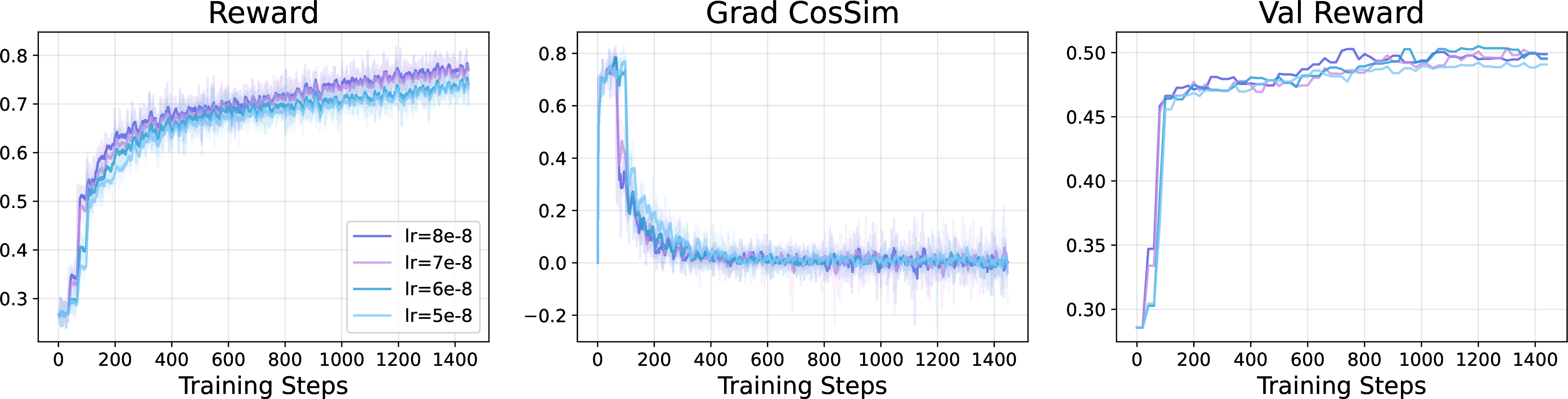
Figure 3 isolates the small-learning-rate regime (\(\eta\in\{8,7,6,5\}\!\times\!10^{-8}\)) on the 3B policy, deliberately trained over an extended horizon of roughly \(1.4\!\times\!10^{3}\) steps—more than twice the window of the main sweep. Here the Grad CosSim rises only briefly during the initial reward climb and then decays toward zero, where it remains for the rest of training: consecutive updates are essentially uncorrelated, so \(\xi_t\) dominates \(\delta_t\) and the learner performs a diffusive walk. This sub-linear (\(\sqrt{t}\eta\)) accumulation is the decisive point: were the drift ballistic, the escape-time law \(t_{\mathrm{collapse}}\eta\approx\text{const}\) would place no lower bound on \(\eta\) below which collapse is forbidden, so even these tiny learning rates would eventually exhaust the horizon budget. Instead, all four runs train stably for the entire extended horizon with monotonically improving validation reward and show no sign of collapse, ruling out a merely-delayed ballistic escape.
The Grad CosSim directly witnesses the decomposition of Eq. 22 : high cosine (coherent \(\delta_t\), ballistic, collapses on the \(t\eta\) horizon) versus near-zero cosine (noise \(\xi_t\) dominates, diffusive \(\sqrt{t}\eta\), stable indefinitely). The extended-horizon stability of small-\(\eta\) runs confirms that small \(S\eta\) does not merely delay collapse—it removes the coherent drift that would cause it.
4.4.0.4 Reconciling the two constraints.
The two regimes are two facets of the same decomposition, and together they instantiate the two-constraint rule \(\eta\ll\min\{R_{\mathrm{batch}}/(S G_{\mathrm{upd}}),\,R_{\mathrm{crit}}/(T G_{\mathrm{upd}})\}\) of Eq. 32 . The local stale-rollout condition \(S\eta\lesssim R_{\mathrm{batch}}/G_{\mathrm{upd}}\) governs whether \(\delta_t\) is large enough to dominate \(\xi_t\) and make the drift coherent; crossing it flips a run from the diffusive (stable) to the ballistic (collapsing) regime, yielding \(\eta_{\max}\propto 1/S\) (§4.2). The horizon-level condition \(T\eta\lesssim R_{\mathrm{crit}}/G_{\mathrm{upd}}\) then governs when a ballistic run reaches the boundary, yielding the \(S\)-independent escape-time law (§4.3). The case \(S=8,\eta=2\!\times\!10^{-7}\) survives not because its horizon budget is unspent, but because its small \(S\eta\) keeps it on the diffusive side of the first constraint, where the escape-time argument does not apply.
5 Related Work↩︎
5.0.0.1 RLHF policy optimization.
RLHF commonly combines supervised fine-tuning, reward modeling, and policy optimization [1]–[3]. PPO-style methods use clipped importance ratios and value baselines [4], while GRPO removes the critic by using group-relative reward statistics [5]. Our analysis focuses on the asynchronous behavior-policy mismatch that arises when such surrogate objectives are optimized using stale rollout batches.
5.0.0.2 Asynchronous and delayed optimization.
Asynchronous SGD has been studied in shared-memory and parameter-server settings [8]–[11], [19]. Those analyses typically model staleness as a bounded delay in gradient computation. In RLHF, the delay also changes the data distribution and the behavior-policy denominator in the policy-ratio surrogate; the resulting bias is therefore not captured by delayed-SGD bounds alone.
5.0.0.3 Decoupled actor-learner architectures in RL.
Decoupling acting from learning is the central design pattern of large-scale distributed RL, from Gorila [12] and A3C [13] to IMPALA [14], Ape-X [15], and SEED RL [16]. A consistent theme is that the throughput gained by decoupling must be paid for in off-policy bias: IMPALA stabilizes high-throughput training only after adding the V-trace off-policy correction [14], while DD-PPO [17] avoids the problem by remaining fully synchronous, and reproducibility studies highlight how stale rollouts perturb actor-learner PPO dynamics [18]. Our setting differs in two respects. First, GRPO-based RLHF [5] relies on clipped importance ratios and KL regularization rather than a dedicated off-policy estimator, so the burden of stability falls on the \((S,\eta)\) configuration itself. Second, rather than proposing a new correction, we characterize when stale rollouts are tolerable, separating a per-step bias controlled by \(S\eta\) from a horizon-level drift controlled by \(T\eta\).
5.0.0.4 Scaling laws and training stability.
Scaling laws for language models relate loss or efficiency to model size, data, compute, and optimization hyperparameters [20]–[22]. This paper studies a complementary scaling interaction between rollout staleness and learning rate in asynchronous policy optimization.
6 Conclusion↩︎
We analyzed asynchronous GRPO training with stale rollout batches by making the behavior policy explicit in the surrogate gradient. The resulting decomposition shows that stale rollouts introduce a per-step surrogate-gradient bias of order \(O(S\eta)\) under local smoothness assumptions. The collapse-time argument should be interpreted conditionally: when within-cycle stale-rollout drift remains below a batch-level clipping radius, the observed collapse horizon is governed primarily by cumulative learner drift \(T\eta\); otherwise, the stable learning rate can depend directly on \(S\eta\). This yields a two-constraint stability rule that reconciles the single-step stale-bias bound with the empirical observation that learning-rate thresholds may appear weakly dependent on staleness in the horizon-limited regime.
7 Relaxing Bounded Updates↩︎
Assumption 1 is a convenient main-text condition. A weaker version can replace the almost-sure update bound with a bounded second moment, for example \[\mathbb{E}\left[\|g(\theta_t;\mathcal{B}_{\phi_t})\|^2\mid \theta_t,\phi_t\right] \le G_2^2.\] Then the expected stale-policy drift obeys \[\mathbb{E}\left[\|\theta_t-\theta_{t-k_t}\|\right] \le \eta k_t G_2 \le \eta S G_2,\] by Jensen’s inequality and the triangle inequality. Under standard sub-Gaussian or clipped-update conditions, the same scaling holds with high probability up to logarithmic factors. Thus the main-text \(O(S\eta)\) staleness scaling is not tied to an almost-sure bound, although the constants and probability statements change.
8 Separate Rewards↩︎

