AutoSpeed: Annotation-Free Stage-Adaptive Motion Speed Learning for Robot Manipulation
July 01, 2026
1 Introduction↩︎
Imitation learning (IL) is widely adopted for visuomotor policy learning. In recent years, it has catalyzed a diverse range of visuomotor policies [1]–[4] for robotic manipulation, including prominent Vision-Language-Action (VLA) models [5]–[8]. Existing IL-based policies typically mimic the motion speed exhibited in expert demonstrations. [9] Regardless of the stage of the task, the policy predicts actions over a fixed future horizon, i.e., it uses fixed-length action chunking [1], [2]. However, the motion speeds in expert demonstrations are often suboptimal, thereby limiting the efficiency and performance of the learned policy. In practical deployment scenarios, task completion efficiency is often critical, especially in industrial settings.
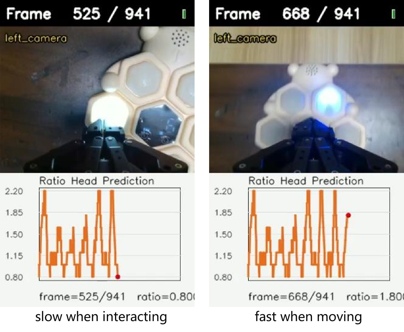
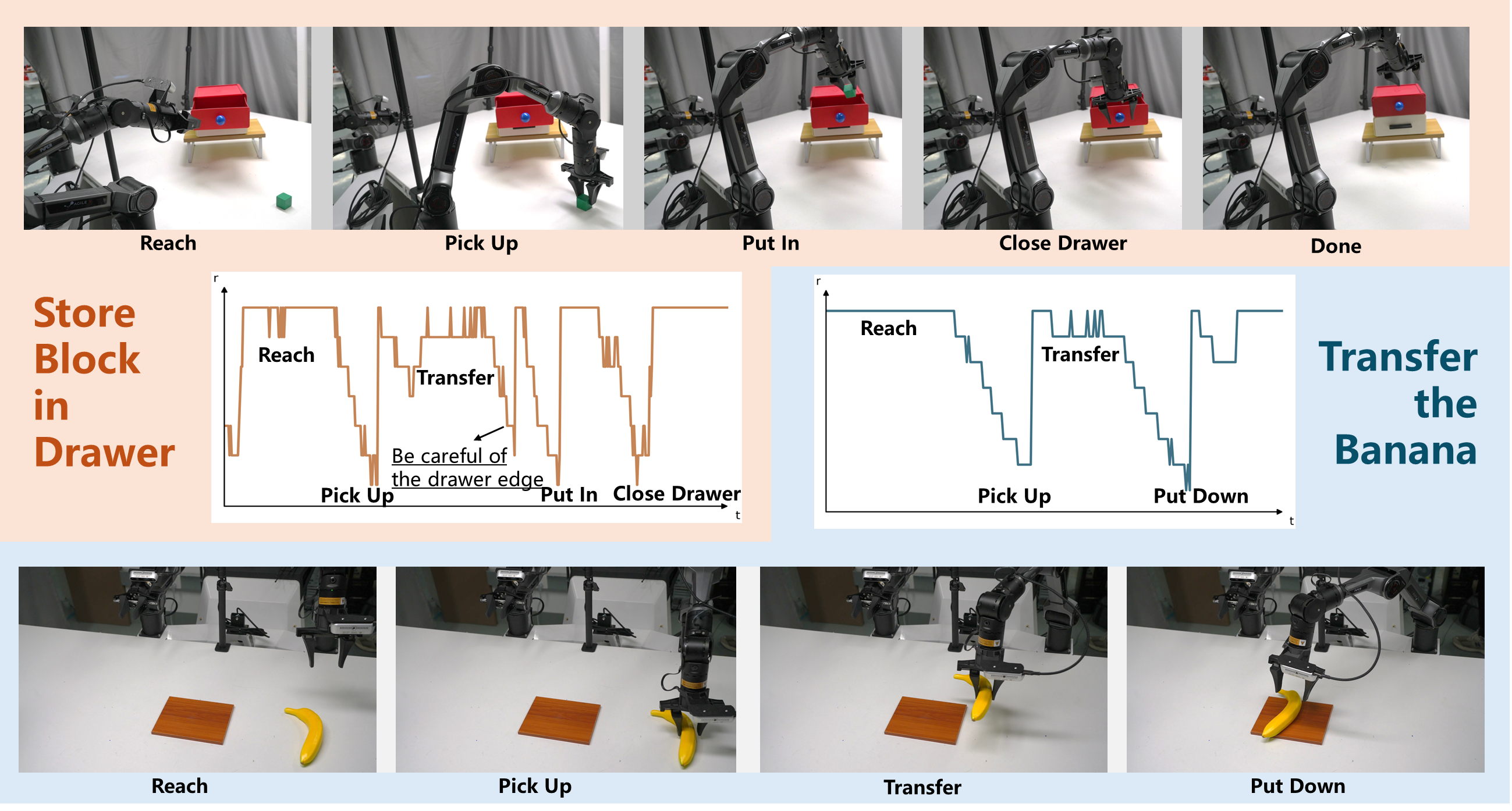
Different stages of manipulation tasks exhibit varying levels of difficulty [10], [11], suggesting that both the motion speed and the temporal prediction horizon should be stage-dependent. Empirically, we find a consistent positive relationship between motion speed and effective prediction horizon, aligning with prior findings in human motor and cognitive control [12], [13]. As shown in Fig. [fig:coarse], in easy stages, such as free-space reaching or coarse repositioning, long-horizon action chunks can be predicted reliably from the current observation [14], [15], allowing faster execution. In contrast, fine-grained stages such as insertion or sustained interaction demand higher precision and tighter perception–action coupling, and are therefore better served by shorter effective prediction horizons and slower execution. This is consistent with findings in human motor and cognitive control: when task demands are low, humans can act faster with relatively little monitoring, whereas precision-critical behaviors require closer feedback monitoring and often slower movements to preserve accuracy [16]–[18].
Building on these motivations, we introduce AutoSpeed, a model-agnostic learning framework that enables existing visuomotor policies to predict trajectories at stage-adaptive motion speeds. In this work, we hypothesize and validate that the stage-dependent speed ratio can be implicitly inferred during end-to-end policy training. This obviates the need to train an additional proxy policy [19] or to rely on VLM-based or manual annotations [20]–[22]. Moreover, AutoSpeed jointly optimizes the quality of implicit speed ratio inference and trajectory prediction in an end-to-end training pipeline.
Concretely, as shown in Fig. [fig:coarse], given a set of speed ratios (e.g., sampled from 0.8 to 2.2 in increments of 0.2), we obtain action chunks at different speeds by applying discrete cosine transform (DCT)[23] to the original trajectories in the frequency domain (section 2.3). This technique enables non-integer speed modulation while preserving more high-frequency action details for fine-grained manipulation[24]. We use fixed-length action chunks to keep the model’s output dimensionality consistent; acceleration compresses trajectories in time and increases the effective horizon, while deceleration expands them and reduces it. We then treat future trajectories at different speeds as a set of candidate supervision targets. Each candidate is evaluated with a composite cost that trades off prediction error against prediction horizon, and we optimize the policy toward the minimum-cost candidate (section 2.2). A lightweight Ratio Head is trained jointly to predict the speed ratio from latent observation features. Additionally, similar to the temporal ensemble [1], we introduce a nonlinear temporal ensemble (section 2.4.2) that outputs actions by combining the speed prediction of the ratio head with multiple overlapping fragment predictions, allowing for smooth deployment at inference time.
Through extensive experiments across diverse simulation benchmarks and real-world tasks, we show that visuomotor policies trained with AutoSpeed consistently reduce task execution time while improving success rates. AutoSpeed supports both single-task and multi-task learning and works across policy classes, spanning non-generative (e.g., MLP-based) and generative (e.g., diffusion- and flow-based) action prediction models. We further demonstrate additional capabilities of AutoSpeed, including controllable motion style and improved policy performance on datasets with substantial demonstration-speed variability. We summarize the contributions of this paper as follows:
We introduce AutoSpeed, which to our knowledge is the first annotation-free, stage-aware framework to implicitly infer motion speed ratios within end-to-end policy learning.
With DCT-based frequency-domain scaling, AutoSpeed enables non-integer acceleration and deceleration while preserving high-frequency action details.
Policies trained with AutoSpeed substantially shorten task completion time while improving success rates. Moreover, the inferred speed ratios are closely aligned with task stages.
2 Method↩︎
2.1 Problem Setup↩︎
Imitation learning for robotic manipulation aims to train a policy by minimizing the prediction error of demonstrated trajectories conditioned on observations. An expert dataset is given as \(\mathcal{D}=\{(l^{(i)}, \tau^{(i)})\}_{i=1}^{N}\), where each trajectory \(\tau\) is denoted by \(\tau=\{(o_t, a_t, s_t)\}_{t=1}^{T}\) and the task instruction \(l\) specifies the task. At each time step \(t\), \(o_t\) denotes the image observation, \(a_t\) denotes the motion control signal, and \(s_t\) denotes the robot state. We denote the chunk size by \(H\), and the observation horizon by \(K\). For brevity, we omit conditioning inputs other than \(\mathbf{o}_{t-K+1:t}\). A standard visuomotor policy \(\pi_\theta\) predicts a length-\(H\) action chunk conditioned on the recent observation context: \[\pi_\theta\!\left(\mathbf{a}_{t:t+H-1}\mid \mathbf{o}_{t-K+1:t}\right).\]
To enable stage-adaptive motion speed learning, the key challenge is to identify which stages in demonstration trajectories can be safely accelerated. We define the motion speed ratio as \(r_t\) at time step \(t\). Larger \(r_t\) corresponds to easier stages, allowing faster execution and a longer temporal prediction horizon; smaller \(r_t\) corresponds to precision-critical stages, demanding slower execution, a shorter horizon and higher-frequency feedback.
In our framework we use a fixed number of chunks to keep the model’s output tensor shape consistent. Therefore, the temporal prediction horizon \(h_t\) is positively correlated with the motion speed ratio \(r_t\). then: \[\mathrm h_t \;=\;{H} \cdot r_t \;\]
Accordingly, a visuomotor policy trained with AutoSpeed is formulated as: \[\pi_\theta\!\left(\mathbf{a'}_{t:t+{h_t}-1},\mid \mathbf{o}_{t-K+1:t}\right).\]
where \(\mathbf{a'}_{t:t+h_t-1}\) has a motion speed \(r_t\) matched to the current task stage. The transformation from \(\mathbf{a}_{t:t+H-1}\) to \(\mathbf{a'}_{t:t+{h_t}-1}\) is described in Sec. 2.3. Besides, Sec. 2.2 details the AutoSpeed optimization procedure. Sec. 2.4 presents training recipes for generative policy classes and introduces a compatible inference-time strategy that aggregates overlapping predictions to improve smoothness. In the following sections, we denote an action chunk by \(A\).
2.2 Multi-Target Selective Optimization↩︎
Recent studies have analyzed and empirically validated quantifiable stage signatures in robotic manipulation: fine-grained behaviors are often reflected in the high-frequency components of action trajectories[24], while the policy’s predicted action entropy can serve as a proxy for identifying difficult, failure-prone stages[19], [25], [26]. We hypothesize that the stage-dependent signal \(r_t\) can be implicitly inferred during end-to-end training, and in this work we validate that it is feasible and model-agnostic. We formulate training as cost-aware multi-target optimization.
2.2.1 Optimization Target Set↩︎
At each time step \(t\), we construct a set of candidate future trajectories at different speeds \(\{r_t^{(m)}\}_{m=1}^M\) , denoted by \(\{A_t^{(m)}\}_{m=1}^M\). AutoSpeed supports a user-defined discrete set of motion-speed ratios (e.g., sampled from 0.8 to 2.2 in increments of 0.2), and \(M\) denotes the number of speed candidates. Compared to manually downsampling demonstrations at only integer-rate factors[19], [20], this design provides greater flexibility and enables smoother speed transitions.
2.2.2 Cost-based Selective Optimization↩︎
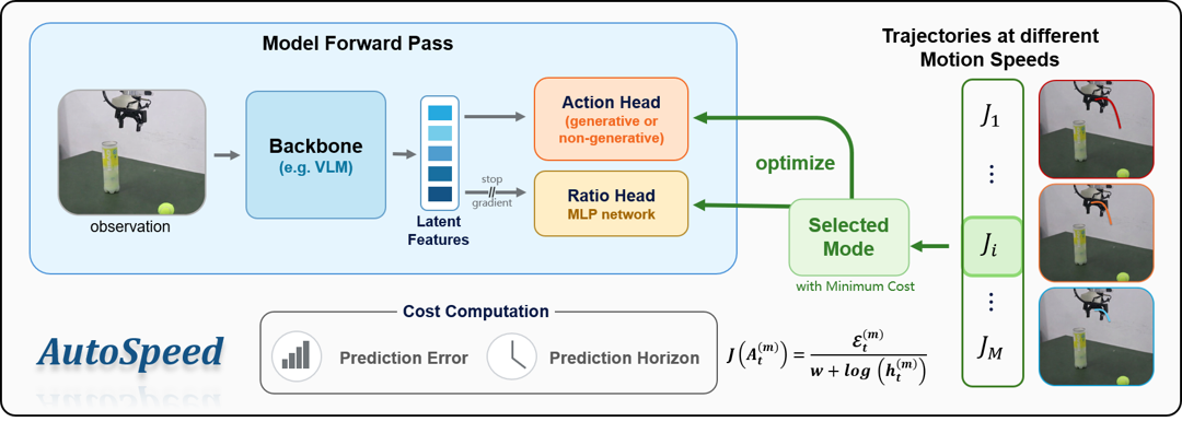
As shown in Fig. 1, the multi-target setting yields a set of losses, each corresponding to an optimization direction. We evaluate these candidates using a composite cost \(J\) that trades off prediction error against temporal prediction horizon: \[J\left({A_t^{(m)}}\right) = \frac{ \mathcal{E}^{(m)}_t }{ w + \log\!\left(h_t^{(m)}\right) }, \label{eq:composite-cost}\tag{1}\]
\(\mathcal{E}^{(m)}_t\) denotes the model’s mean-squared prediction error (MSE) for candidate \(m\) at time \(t\). For non-generative models, \(\mathcal{E}^{(m)}_t\) reduces to the MSE between the predicted action chunk and \(A_t^{(m)}\). For generative models, \(\mathcal{E}^{(m)}_t\) can be instantiated as an MSE either on the denoising target (i.e., the injected noise) or directly on the ground-truth actions[27], with the former being more commonly used[2], [7], [28]. The denominator serves as an adaptive normalization term. Candidates with shorter prediction horizons receive a larger penalty, encouraging the model to favor well-predicted futures while selecting faster speeds whenever possible. Intuitively, in easier stages, future actions remain predictable over longer horizons, permitting higher speed ratios; in precision-critical stages, long-horizon prediction becomes less predictable, yielding lower speed ratios. Additionally, \(w\) is a constant term that can be tuned to control motion style. A smaller \(w\) biases the policy toward a more aggressive motion style. We examine the sensitivity of the results to this setting in Sec. 3.6.2.
We then select the minimum-cost candidate:
\[m^\star = \arg\min_{m\in\{1,\dots,M\}} J\!\left({\mathbf{A}}^{(m)}\right) \label{eq:target-selection}\tag{2}\]
AutoSpeed trains the policy by minimizing the loss on the selected target, \[\min_{\theta}\; \mathbb{E}_{\tau\sim\mathcal{D}} \left[ \sum_{t} \mathcal{L}_\theta\!\left(\mathbf{o}_{t-K+1:t},\, \mathbf{A}^{(m^{\star)}}\right) \right]. \label{eq:elasticmotion-objective}\tag{3}\]
2.2.3 Criterion for different models.↩︎
AutoSpeed is model-agnostic. For policies with non-generative action heads, the model output is the action prediction; therefore, we set \(\mathcal{E}^{(m)}_t\) to the mean-squared error (MSE) of the predicted actions.
For diffusion-based action heads, the action chunk \(A_t^{(m)}\) serves as the generation target and is progressively corrupted by Gaussian noise \(\boldsymbol{\epsilon}\sim\mathcal{N}(\mathbf{0},\mathbf{I})\) during training to obtain a noised sample \(\mathbf{x}^{(m)}_\kappa\) at diffusion step \(\kappa\); the denoiser \(\epsilon_\theta(\cdot)\), conditioned on the observation context \(\mathbf{o}_{t-K+1:t}\), learns to predict the injected noise. Therefore, we set \(\mathcal{E}^{(m)}_t\) to the mean-squared error (MSE) of the predicted noise: \[\mathcal{E}^{(m)}_t = \mathbb{E}_{\boldsymbol{\epsilon}\sim\mathcal{N}(\mathbf{0},\mathbf{I}),\,\kappa} \left[ \left\| \boldsymbol{\epsilon}- \epsilon_\theta\!\left(\mathbf{o}_{t-K+1:t},\,\mathbf{x}^{(m)}_\kappa,\,\kappa\right) \right\|_2^2 \right], \label{eq:Em-diff}\tag{4}\]
For flow-matching-based action heads, the model learns a conditional velocity field \(v_\theta(\cdot)\) that transports a noise sample \(\boldsymbol{\epsilon}\) to the target action chunk \(A_t^{(m)}\) along an interpolation \(\mathbf{x}^{(m)}_\tau=(1-\tau)\boldsymbol{\epsilon}+\tau A_t^{(m)}\), where \(\tau\in[0,1]\) is the interpolation time. Accordingly, we set \[\mathcal{E}^{(m)}_t = \mathbb{E}_{\tau\sim \mathcal{U}(0,1),\,\boldsymbol{\epsilon}\sim\mathcal{N}(\mathbf{0},\mathbf{I})} \left[ \left\| v_\theta\!\left(\mathbf{o}_{t-K+1:t},\,\mathbf{x}^{(m)}_\tau,\,\tau\right) - \left(A_t^{(m)}-\boldsymbol{\epsilon}\right) \right\|_2^2 \right]. \label{eq:Em-flow}\tag{5}\]
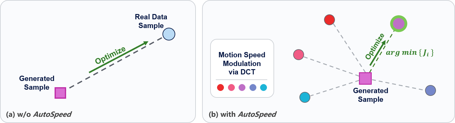
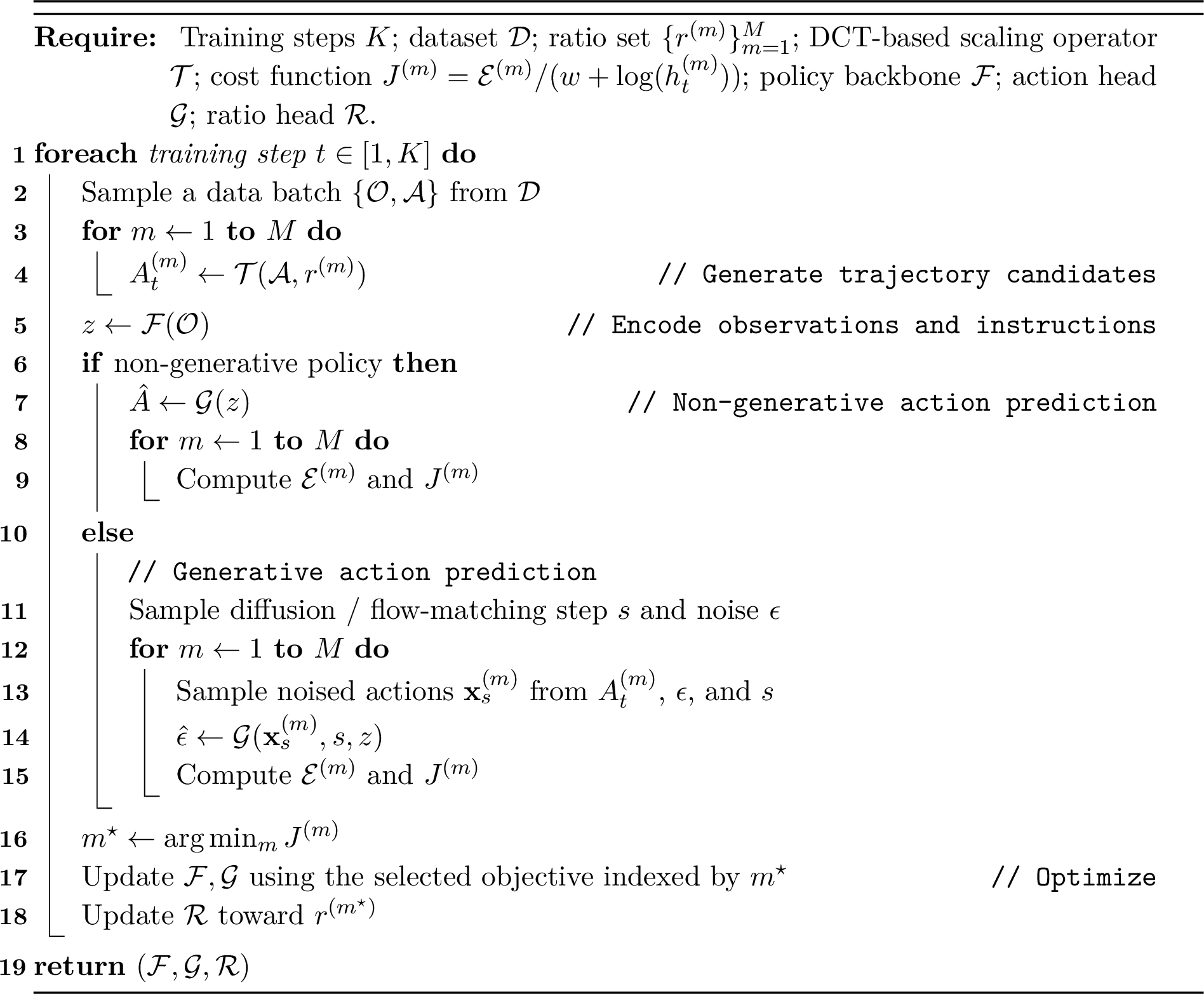
As shown in Fig. 2, AutoSpeed extends the general mechanism to generative action heads by constructing multiple speed-modulated generation targets for each training sample. At each denoising or flow-matching prediction step, the model is no longer constrained to match a single fixed target; instead, it performs Multi-Target Selective Optimization by selecting the candidate with the minimum cost.
2.2.4 Ratio Head.↩︎
We introduce a lightweight Ratio Head trained to predict the speed ratio \(r_t\) from latent observation features. It provides stage-adaptive motion speeds in the third stage of generative-model training 2.4.1, and its predictions are used by the Nonlinear Temporal Aggregation (NTA) module 2.4.2 during inference.
2.3 Motion Speed Transform↩︎
We apply the discrete cosine transform (DCT) [23] to map time-domain action signals into the frequency domain, perform temporal scaling there to realize stretching/compression along the time axis, and then transform the actions back to the time domain.
In details, we first compute DCT-II coefficients of the original action chunk \(A\in\mathbb{R}^{H_0\times D}\) along the temporal axis, where \(H_0\) denotes the maximum number of action samples required: \[\mathbf{C}=\mathrm{DCT}\!\left(A\right)\in\mathbb{R}^{H_0\times D}\]
We then retime by evaluating the inverse-DCT basis at the speed ratio \(r\) and reconstruct the retimed chunk via a basis–coefficient product: \[\tilde{A}=\mathbf{B}(r)\mathbf{C},\qquad \mathbf{B}(r)_{i,k}=\sqrt{\frac{2}{H_0}}\,\alpha_k\cos\!\Big(\frac{\pi k (t_i+0.5)}{H_0}\Big),\] where \(t_i=i\cdot r\) for \(i=0,\dots,H-1\), \(k=0,\dots,H_0-1\), \(\alpha_0=1/\sqrt{2}\), and \(\alpha_k=1\) for \(k\ge 1\). During training, the candidates \(\{{A}^{(m)}\}_{m=1}^{M}\) are generated by applying the operator with the speed ratio set \(\{r^{(m)}\}_{m=1}^{M}\).
This enables both acceleration and deceleration with non-integer scaling factors, while the frequency-domain processing effectively preserves high-frequency details that are crucial for fine-grained manipulation[24].
2.4 Other Techniques↩︎
2.4.1 Training Recipe for Generative Models↩︎
In practice, we find across multiple training and testing runs that even when using Multi-Target Selective Optimization throughout the entire process, the model can still learn favorable speed profiles and achieve strong performance.
To further improve training stability for generative models and reduce the additional computational cost, we propose a three-stage training strategy:
Inspired by [29], which shows that diffusion models tend to preferentially learn smooth, low-complexity, and generalizable structure in the early stages of training, we optimize the model in the early training stage by minimizing the average loss over all candidates. The second stage corresponds to the multi-objective optimization process (Sec. 2.2). In the third stage, the Ratio Head is frozen, and the model is optimized directly using the motion speed predicted by the Ratio Head, allowing the remaining steps in the generation process to rapidly converge to the selected mode. This provides a training optimization direction for scaling to larger datasets.
2.4.2 Nonlinear Temporal Aggregation↩︎
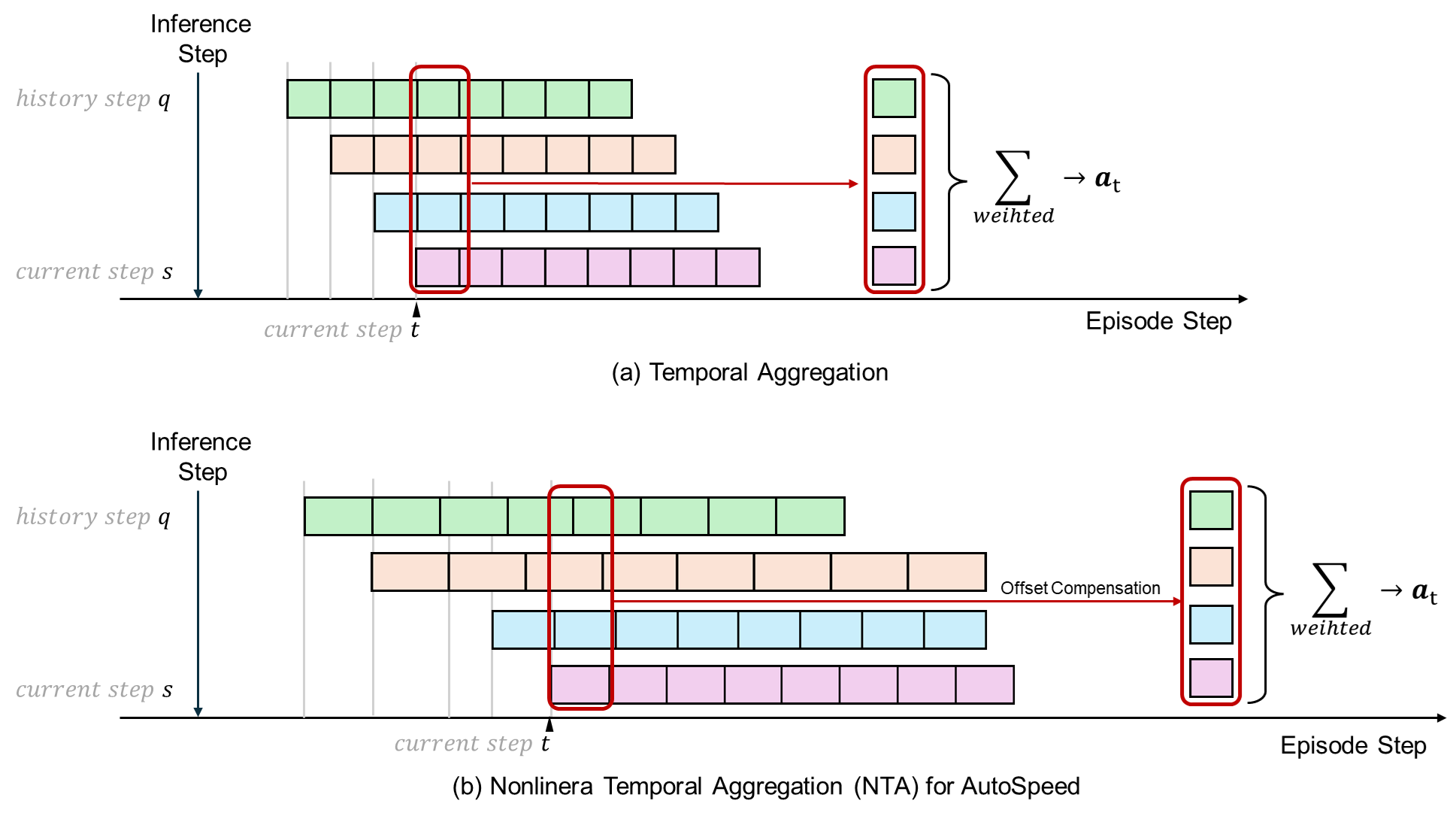
Conventional temporal aggregation assumes uniform time intervals consecutive actions across all chunks, rendering it incompatible with the variable-speed predictions generated by AutoSpeed. To address this limitation, we introduce Nonlinear Temporal Aggregation (NTA), a novel mechanism that enables the ensembling of overlapping prediction across action chunks operating at different temporal scales.
NTA computes a weighted average of actions from multiple chunks within a predefined time window. Specifically, at a given control step \(s\) (denoted temporally as \(t=0\)), all predicted actions from previously generated chunks that fall within the time window \([-i,+i]\) are collected. Then, we compute a weighted average of the candidate actions using an exponential-decay weighting scheme and slight temporal misalignment is also corrected via the same frequency-domain transformation. We provide the details of NTA in the appendix.
3 Evaluation↩︎
Our evaluations aim to investigate and answer the following questions:
Can AutoSpeed effectively reduce the time required to complete tasks while maintaining task success rates?
Can the inferred speed ratios produced by AutoSpeed effectively indicate different task stages?
Is AutoSpeed effective in both single-task and multi-task learning settings, and does it work for both non-generative and generative models?
3.1 Experimental Setup↩︎
We evaluate AutoSpeed across a range of standard manipulation benchmarks and real-world tasks.
3.1.1 Simulation Tasks:↩︎
We experiment with two bimanual tasks from the ALOHA benchmark [1], 10 tasks from the LIBERO-10 suite [30], 50 tasks from the Meta-World benchmark [31], shown in Fig. 4. In ALOHA simulation, we evaluate the Transfer Cube and Insertion tasks, utilizing 50 expert demonstrations per task. For both the LIBERO-10 suite and the Meta-World benchmark, the policies are trained using 50 expert demonstrations per task under a multi-task learning paradigm.
3.1.2 Real-world Tasks:↩︎
We conduct real robot experiments on an Agilex Piper bimanual robot platform in a tabletop manipulation environment. The policies are trained on RGB images and robot proprioceptive state. The images are captured via two wrist cameras mounted on the top of the grippers and one fixed camera installed on top of the table. The action space comprises the joint states and the gripper state. Using a teleoperation system, we collect a dataset for four distinct tabletop tasks, with each task comprising approximately 50 expert demonstrations. Notably, the expert action trajectories are temporally oversampled by a factor of 2, enabling fine-grained actions when deploying deceleration.
![Figure 4: Simulation Tasks. We select a total of 62 tasks from ALOHA Sim[1], MetaWorld[31], and LIBERO-Long[30], and use 50 demonstration trajectories for each task.](/article/2607.01051/figures/SimTasks.png "fig:")
3.1.3 Models↩︎
We compare policies optimized with our AutoSpeed framework against their vanilla counterparts trained with original objectives.
3.1.3.1 ACT
: Action Chunking Transformer(ACT) [1] is a visuomotor policy composed of a transformer encoder and decoder. We use it as a representative non-generative baseline model.
3.1.3.2 BAKU
: BAKU[3] is a transformer-based architecture designed for multi-task learning. This architecture is highly representative: most existing visuomotor policies, including VLA models, are largely built upon an Observation Encoder–Backbone–Action Head design. It employs a transformer encoder to fuse information from different modalities and trains a decoupled action head to generate action chunks. This modular design enables the action head to be readily substituted with several generative variants.
We use these from-scratch models to isolate the contribution of AutoSpeed and show that its effectiveness does not depend on capabilities inherited from large-scale pretraining. AutoSpeed can also be applied to training or fine-tuning larger-scale models. Moreover, after applying AutoSpeed once to a training dataset, the inferred stage-aware motion speed annotations can be stored and reused, thereby avoiding repeated Multi-Target Selective Optimization in future training or fine-tuning pipelines.
3.1.4 Metrics↩︎
In addition to the standard metric of task success rate, we report the average episode length of successful rollouts to assess overall execution efficiency. For the Aloha benchmark, we perform 50 evaluation rollouts per task. For both the LIBERO-10 suite and the Meta-World benchmark, we adopt a consistent evaluation protocol, executing 10 trials per task and reporting the aggregated success rates and execution length. For the real-world evaluation, we report the task success rate and average completion time (in seconds) across 20 trials per task, with a weighted success rate computed over individual subtask stages.
3.2 Main Results on Single-Task Learning Simulation↩︎
Table 1 summarizes the quantitative results evaluated on the ALOHA benchmark.
Compared to the vanilla ACT baseline, the policy trained with AutoSpeed (denoted as AutoSpeed) achieves a substantial reduction in task execution time without compromising overall performance. Specifically, on the Transfer Cube task, AutoSpeed reduces the average episode length from 272 to 160 steps, yielding a maximum speedup of 1.7x. While this accelerated execution slightly lowers the success rate (from 72% to 64%) under standard control due to the heightened sensitivity of high-speed interactions, coupling AutoSpeed with a high-gain controller effectively mitigates this issue. This combination not only preserves the execution efficiency but also surpasses the original baseline with a 6% improvement. Furthermore, on the contact-rich Insertion task, AutoSpeed simultaneously improves the success rate (from 22% to 24%) and reduces execution length (from 353 to 296 steps with high-gain), demonstrating its robust execution efficiency in single-task learning scenarios.
| Method | Transfer Cube | Insertion | ||
|---|---|---|---|---|
| 2-3 (lr)4-5 | SR (\(\uparrow\)) | Len (\(\downarrow\)) | SR (\(\uparrow\)) | Len (\(\downarrow\)) |
| ACT | 72% | 272 | 22% | 353 |
| ACT(AutoSpeed) | 64% | 160 | 24% | 300 |
| ACT(AutoSpeed\(^{\dagger}\)) | 78% | 165 | 24% | 296 |
3.3 Main Results on Multi-Task Learning Simulation↩︎
The quantitative results on the LIBERO-10 and Meta-World benchmark are presented in Table 2. AutoSpeed consistently outperforms the strongest baselines across both multi-task benchmarks. On Meta-World, AutoSpeed yields substantial improvements in success rates regardless of the underlying action head: BAKU-DiT exhibits a 19.0% increases, while BAKU-Flow improves by 7.8% to achieve the highest overall success rate (65%). Crucially, these gains are accompanied by marked reductions in average episode lengths. On the LIBERO-10 suite, AutoSpeed-trained policy compresses the execution time with a maximum acceleration of approximately 40% to its vanilla counterpart. Compared to baselines that naively execute actions at a fixed, dataset-dictated speed, AutoSpeed’s stage-adaptive optimization empowers policies to complete tasks substantially faster, while simultaneously improving success rates by dynamically adjusting to the complexity of the current task phase.
Crucially, our experiments demonstrate that reducing task execution time and improving success rates are not mutually exclusive. By predicting trajectories at stage-adaptive motion speeds, AutoSpeed leverages long-horizon action chunks for faster execution during easy stages, where future actions can be predicted reliably. Conversely, during fine-grained stages that demand tighter perception-action coupling, the framework naturally adopts slower execution and shorter effective horizons to preserve control accuracy. Because this stage-aware modulation is implicitly inferred during end-to-end training via our composite cost, AutoSpeed generalizes effectively across multi-task scenarios, delivering superior execution efficiency while preserving task success compared to baselines.
| Method | LIBERO-10 | Meta-World | ||
|---|---|---|---|---|
| 2-3 (lr)4-5 | SR (\(\uparrow\)) | Len (\(\downarrow\)) | SR (\(\uparrow\)) | Len (\(\downarrow\)) |
| BAKU-DiT | 50% | 261 | 43% | 87 |
| BAKU-Flow | 47% | 287 | 57% | 82 |
| BAKU-DiT (AutoSpeed) | 49% | 259 | 62% | 70 |
| BAKU-Flow (AutoSpeed) | 52% | 171 | 65% | 71 |
4pt
3.4 Main Results on Real-World Tasks↩︎
As shown in Table 3, AutoSpeed consistently outperforms the baselines across all evaluated real-world tasks with various length and difficulty levels. Most notably, when integrated with our proposed Nonlinear Temporal Aggregation (NTA), the AutoSpeed-trained policy significantly reduces execution time, delivering an average speedup of approximately 1.78\(\times\) across the diverse task suite.
Crucially, this substantial acceleration does not compromise manipulation precision but yields consistent absolute improvements in task success rates. As illustrated in Fig. 5, in the highly challenging Place the Toy task, AutoSpeed increases the success rate by a notable 10%. These physical deployments further validate AutoSpeed’s capacity to autonomously extract stage-dependent motion speed patterns from unannotated demonstrations. By leveraging the proposed multi-target optimization, the policy translates these learned patterns into superior task efficiency and robust real-world performance.
As shown in Table 4, since action oversampling is practically feasible (easy to reach over 100 Hz), it serves as an optional way to improve fine-grained action fidelity under AutoSpeed, enabled by DCT-based retiming.
| Method | Transfer the Banana | Place the Toy | |||
|---|---|---|---|---|---|
| 2-3 (lr)4-5 | SR (\(\uparrow\)) | Time (\(\downarrow\)) | SR (\(\uparrow\)) | Time (\(\downarrow\)) | |
| BAKU-Flow+TA | 77% | 20.80s | 33% | 18.13s | |
| BAKU-Flow (AutoSpeed)+NTA | 83% | 11.24s | 43% | 10.13s | |
| Method | Stacking Two Cubes | Store Block in Drawer | |||
| SR (\(\uparrow\)) | Time (\(\downarrow\)) | SR (\(\uparrow\)) | Time (\(\downarrow\)) | ||
| BAKU-Flow+TA | 60% | 50.11s | 77% | 38.67s | |
| BAKU-Flow (AutoSpeed)+NTA | 63% | 28.52s | 80% | 23.01s | |
4pt
| Real-world 4 Tasks | 1\(\times\) Sampling | 2\(\times\) Sampling | Baseline |
|---|---|---|---|
| Avg. Time (s) (\(\downarrow\)) | 19.41 | 18.23 | 31.93 |
| Avg. SR (%) (\(\uparrow\)) | 65.50 | 67.25 | 61.75 |
5pt
3.5 Training Overhead↩︎
For non-generative models, applying AutoSpeed introduces no additional model computation overhead. For generative models, AutoSpeed incurs a small additional computational cost because the model’s action head needs to denoise each noise-perturbed trajectory candidate.
However, this overhead is limited for two reasons. We report the wall-clock training times across benchmarks in Table 5. First, the parameters of the action head typically constitute only a small fraction of the overall model[3], [6], [8]. Second, the denoising of different trajectory candidates can be performed in parallel[32], [33], which prevents the training process from being significantly slowed down.
All policy training and evaluation procedures are conducted on the NVIDIA A100 GPU. The approximate wall-clock training times for our experiments are presented in Table 5.
| Method | ALOHA | LIBERO-10 | Meta-World | Real-World | |||
|---|---|---|---|---|---|---|---|
| 2-3 (lr)4-5 (lr)6-7 (lr)8-8 | Transfer | Insertion | Flow | DiT | Flow | DiT | Flow |
| Vanilla | 7.6 | 7.6 | 6.2 | 6.5 | 8.0 | 7.2 | 10.1 |
| AutoSpeed | 7.9 | 7.8 | 7.8 | 7.7 | 8.2 | 8.0 | 12.4 |
5pt
3.6 Ablation Studies↩︎
3.6.1 Speed Range↩︎
We evaluate how different predefined speed ranges impact the model’s ability to learn phase-dependent motion patterns and its overall task performance. Specifically, we train the ACT policy equipped with AutoSpeed on the ALOHA Transfer Cube task under three distinct speed range settings: AutoSpeed [1x, 2x], AutoSpeed [1x, 4x], and AutoSpeed [2x, 4x]. All other hyperparameters remain identical for a fair comparison, and a vanilla ACT model is evaluated as the baseline. Note that while this ablation uses a reduced image resolution compared to the main experiments, the same resolution and all other hyperparameters are kept identical across all variants to ensure a fair comparison.
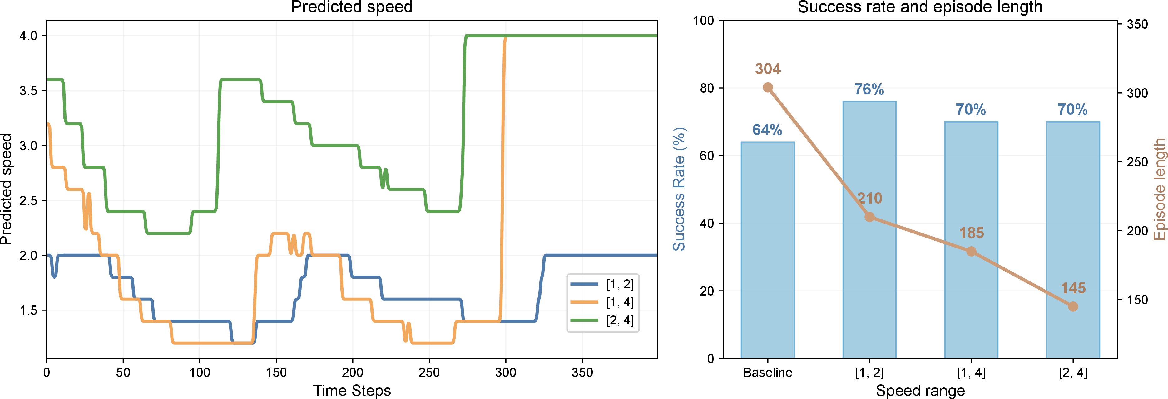
As illustrated in Fig. 6 (left), despite the varying upper and lower bounds, the learned speed trajectories across all three variants exhibit a remarkably consistent phase-aware pattern. The policies autonomously decelerate (forming a valley in the speed curve) during complex, interaction-critical task phases, and accelerate during simpler, unconstrained stages.
Furthermore, Fig. 6 (right) demonstrates that all three AutoSpeed variants consistently outperform the vanilla baseline in both success rate and execution efficiency. Notably, the results reveal a clear tradeoff dictated by the speed bounds: the more conservative [1x, 2x] setting achieves the highest success rate (76% vs. the baseline’s 64%), while the aggressive [2x, 4x] setting maximally minimizes the episode length (dropping from 304 to 145 steps) while still maintaining a highly competitive success rate of 70%.
3.6.2 Sensitivity to \(w\)↩︎
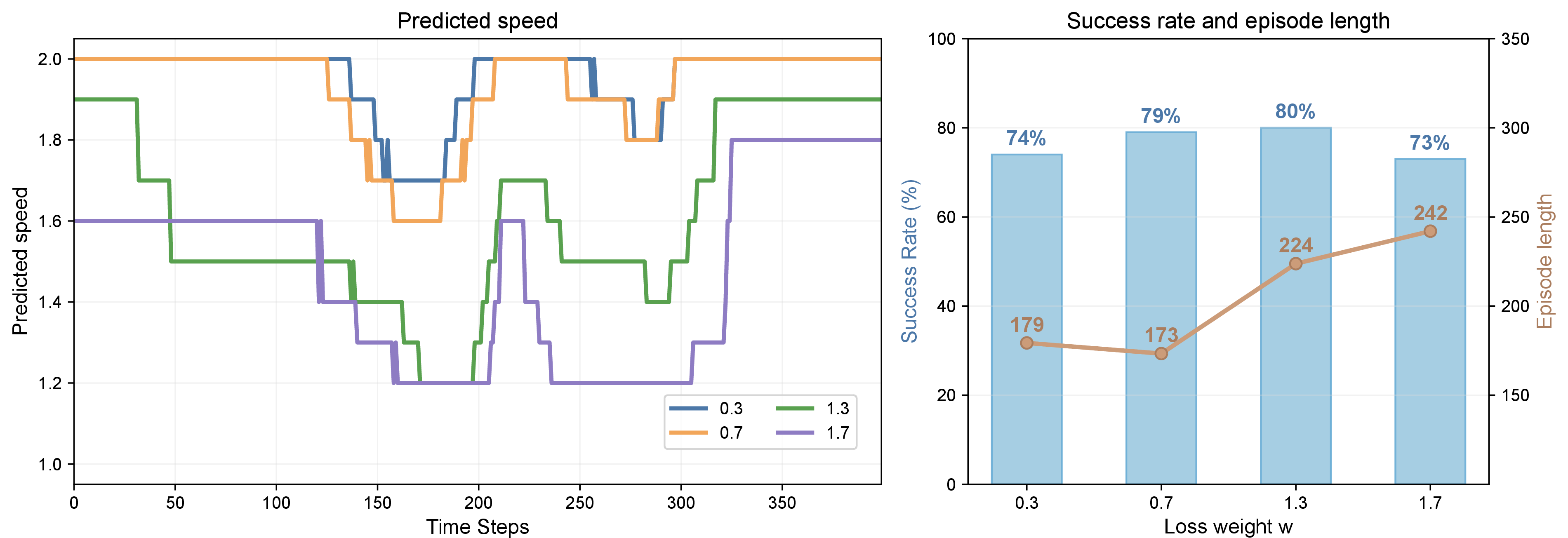
The speed range and \(w\) are both practical design choices for specific task requirements. Different length penalty coefficients inherently shift the model’s preference for speed selection. As the penalty decreases, the relative cost of predicting shorter action chunk increases. Consequently, the model is penalized more heavily for selecting slower speeds and tends to predict action chunk with longer horizons. Fig. 7 shows as policy trained with a smaller length penalty favors generating action chunk with higher speed. Overall, different choices share the phase-aware pattern: the policy accelerates in predictable stages and decelerates in critical interaction stages.
4 Conclusion↩︎
AutoSpeed is a simple yet effective training paradigm for learning stage-adaptive motion speed and temporal prediction horizon directly from standard expert demonstrations. Rather than relying on external annotations or post-hoc trajectory retiming, AutoSpeed uncovers an endogenous signal \(r_t\) during end-to-end policy learning by selecting, among re-timed candidate futures, the target that best balances prediction error and temporal prediction horizon. This unifies speed control and temporal reasoning under a single objective and is compatible with both non-generative and generative visuomotor policies. Across a broad suite of simulation and real-world manipulation tasks, AutoSpeed improves efficiency while maintaining success rates. We hope AutoSpeed offers a practical and broadly applicable route toward faster, safer, and more reliable visuomotor policy deployment.
We provide further details on the following aspects:
The AutoSpeed Training Procedure.(Sec. 5)
Related Works.(Sec. 6)
The Experimental Hyperparameter Settings and Training Details.(Sec. 7)
Implementation Details of Nonlinear Temporal Aggregation.(Sec. 8)
Main Failure Modes for Adaptive-Speed Manipulation.(Sec. 9)
Connection and Comparison with Action Entropy.(Sec. 10)
More AutoSpeed-Identified Speed Ratio Curves.(Sec. 11)
5 The AutoSpeed Training Procedure↩︎
We present the AutoSpeed training procedure to clarify how training differs across model classes and to illustrate the selective optimization process.
6 Related Work↩︎
6.1 Motion Speed Modulation in Robot Manipulation↩︎
We categorize the literature on motion speed modulation in robot manipulation by when the motion speed ratio is inferred: (1) pre-training inference, where it is inferred before training and used to annotate the dataset; (2) test-time inference, where it is inferred during model deployment; and (3) training-time emergence from unlabeled data, where it is implicitly inferred during end-to-end training.
The following methods fall into the first category: DemoSpeedUp [19] derives safe-to-accelerate regions by estimating action entropy with a proxy policy, and retrains a faster policy on the annotated dataset. Similarly, ESPADA [20] uses VLM/LLM-based stage annotations to identify the safe-to-accelerate regions. Moreover, SpeedAug [34] constructs tempo-augmented trajectories to learn a tempo-enriched imitation prior, then applies RL-based fine-tuning to push toward faster policies. And the following methods fall into the second category: SAIL [35] integrates complexity-aware speed modulation with high-gain tracking and scheduling to safely increase execution speed, while SRIL [36] reduces computing latency by learning when to skip inference. VFIL [37] treats speed as an explicit command and conditions the policy on sampling frequency, enabling variable-speed execution by changing the control frequency at deployment without retraining.
However, the third paradigm remains underexplored despite its practical importance. Annotation-based approaches face two key limitations. First, introducing external tools or training additional models to produce annotations is costly and often requires task-specific heuristics or rules. Second, annotation quality and cross-trajectory consistency directly affect the final policy performance, yet these annotations are not optimized end-to-end with the policy. Moreover, prior work largely focuses on when to accelerate; in AutoSpeed, we unify acceleration and deceleration within a single speed-modulation perspective.
6.2 Flexible Reconfiguration of Action Chunking↩︎
Action chunking, which models the joint distribution of future actions conditioned on past states, is a standard practice in robotic manipulation [1], [2]. While action chunking strengthens temporal consistency and mitigates error accumulation, long chunks reduce access to the most recent observations during execution and thus limit reactivity [14]. A growing body of work shows that the prediction horizon in action chunking can substantially impact policy performance, suggesting the existence of an optimal horizon [14], [38], [39]. Embodied manipulation is inherently stage-structured: predictability and feedback requirements vary substantially across stages, so a single global optimal horizon is at best an average-case compromise. A more appropriate view is local optimality, where the effective horizon should be adapted to the current context during policy prediction or execution.
From the training-time perspective, MoH [40] formulates action chunking as a mixture over multiple horizons, processes them in parallel with a shared action transformer, and fuses the outputs via a gating module. From the inference-time perspective, AutoHorizon [38] adjusts the execution horizon online based on the model’s attention weights. GBC [41] improves diffusion-based behavior cloning via self-guidance adaptive chunking mechanism that selectively refreshes action chunks when higher reactivity is needed.
The shared motivation between motion speed modulation and action chunking reconfiguration is to move beyond a single globally tuned trade-off toward stage-aware, locally optimal adaptation across task stages. Dynamic adjustment of the prediction horizon covered by action chunks is also one of our motivations, and we find it is strongly positively correlated with motion-speed modulation across task stages. Accordingly, we keep the output chunk size fixed to preserve architectural compatibility, and use motion-speed modulation to induce a coupled change in the effective inference horizon, enabling stage-adaptive temporal reasoning without altering the model output dimensionality.
7 Experiment Details and Hyperparameters↩︎
This section provides comprehensive details regarding the experimental setup and hyperparameters utilized across both simulation and real-world evaluations.
The complete list of training hyperparameters is summarized in Table 6. To ensure a strict and fair comparison, the hyperparameter configuration within each specific setting is kept entirely identical between the AutoSpeed-augmented policies and their respective vanilla baselines.
| ALOHA | LIBERO-10 | Meta-World | Real-World | ||||
|---|---|---|---|---|---|---|---|
| 2-3 (lr)4-5 (lr)6-7 (lr)8-8 | Transfer | Insertion | Flow | DiT | Flow | DiT | Flow |
| Chunk Size | 32 | 32 | 32 | 32 | 16 | 16 | 32 |
| Total Steps | 80K | 80K | 300K | 300K | 400K | 400K | 120K |
| Batch Size | 16 | 16 | 128 | 64 | 128 | 128 | 64 |
| LR | \(1\times10^{-4}\) | \(1\times10^{-4}\) | \(1.4\times10^{-4}\) | \(1.4\times10^{-4}\) | \(1\times10^{-4}\) | \(1\times10^{-4}\) | \(1\times10^{-4}\) |
The hyperparameters specific to the AutoSpeed framework are detailed in Table 7. The speed range defines the boundaries within which the policy can optimize the motion speed, while the speed step determines the discrete granularity of the candidate speeds. The speed sets used in these tasks are specified empirically. In AutoSpeed, these settings are treated as user-defined hyperparameters that can be adjusted as needed, allowing the model to exhibit different behaviors and performance characteristics. As shown in the distillation experiments in the main paper, AutoSpeed demonstrates stable performance across different hyperparameter settings.
| ALOHA | LIBERO-10 | Meta-World | Real-World | ||||
|---|---|---|---|---|---|---|---|
| 2-3 (lr)4-5 (lr)6-7 (lr)8-8 | Transfer | Insertion | Flow | DiT | Flow | DiT | Flow |
| Speed Range | [1.0, 2.0] | [0.8, 1.5] | [1.0, 2.0] | [1.0, 2.0] | [1.0, 2.0] | [1.0, 2.0] | [0.8, 2.2] |
| Speed Step | 0.1 | 0.1 | 0.2 | 0.2 | 0.2 | 0.2 | 0.2 |
| Penalty | 1.3 | 1.2 | 1.3 | 1.3 | 1.3 | 1.3 | 2.0 |
8 Implementation details of Nonlinear Temporal Aggregation.↩︎
Temporal aggregation (also called temporal ensembling) is an inference-time mechanism originally introduced alongside action chunking [1] to make closed-loop execution smoother and more reactive without changing the policy architecture. For the current timestep \(t\), multiple past queries provide multiple predictions of the same action \(a_t\); the executor then computes a weighted average over these candidates using an exponential decay scheme (e.g., \(w_i=\exp(-m i)\)), where \(m\) controls how quickly new predictions override older ones. AutoSpeed extends this idea to the speed-adaptive setting. Because AutoSpeed retimes each predicted chunk with a stage-aware speed ratio \(r_t\), overlapping chunks are no longer aligned on a uniform time grid, making conventional temporal aggregation (which assumes equal step intervals) incompatible.
We therefore propose Nonlinear Temporal Aggregation (NTA), which aggregates overlapping predictions produced by a model trained with AutoSpeed. In our setting, task progress is no longer assumed to advance linearly. We use the task progress in the expert trajectory as the reference, denoted by the episode step \(t\). At the next step, the task will advance by \(r_t\) rather than 1. To aggregate overlapping predictions, for each previous chunk predicted at inference step \(q\) that still covers the next episode step \(t+r_t\) under its effective episode horizon \(h_q\), we take into consider the actions within the relative time window \([-i,i]\).
We then assign each candidate action \(a_q\) an exponential-decay weight according to its recency, including the first action from the current predicted action chunk: \[w_q=\exp \;\!\bigl(-m(s-q)\bigr)\] where \(s\) is the current inference step and \(m\) controls how fast recent predictions override older ones. We then normalize these weights to obtain the weighting coefficient \[\tilde{w}_q=\frac{w_q}{\sum_i w_i}\].
For each candidate action \(a_q\), we denote by \(\delta t_a\) its deviation in task progress from the current step. We then apply a frequency-domain transformation to the original action chunk from which \(a_q\) is drawn, yielding an aligned action \(a_q'\) that compensates for this temporal offset.
Let \(\mathcal{Q}_t\) denote the set of all candidate actions. The final action is computed by weighted averaging: \[a_t=\sum_{q\in\mathcal{Q}_t}\tilde{w}_q\,a_q',\]
9 Main Failure Modes for Adaptive-Speed Manipulation.↩︎
(1) Delayed controller response.
Under accelerated execution, rapidly changing actions may exceed the tracking capability of the low-level controller. As supported by Table 1 in the main paper, accelerated execution benefits from a higher-gain controller.
(2) Distortion under sub-\(1\times\) deceleration.
When executing below \(1\times\) speed, frequency-domain retiming may introduce distortion. One optional solution is action oversampling as shown in 4.
(3) Coupled pick-up–lifting transition.
The policy may occasionally start lifting before the grasp is fully stabilized. This is often recoverable by re-grasping, but leaves room for improvement.
(4) Over-aggressive \(w\) or speed bounds.
We will explore adaptive \(w\) and refined retiming in our future work.
10 Connection and comparison with action entropy↩︎
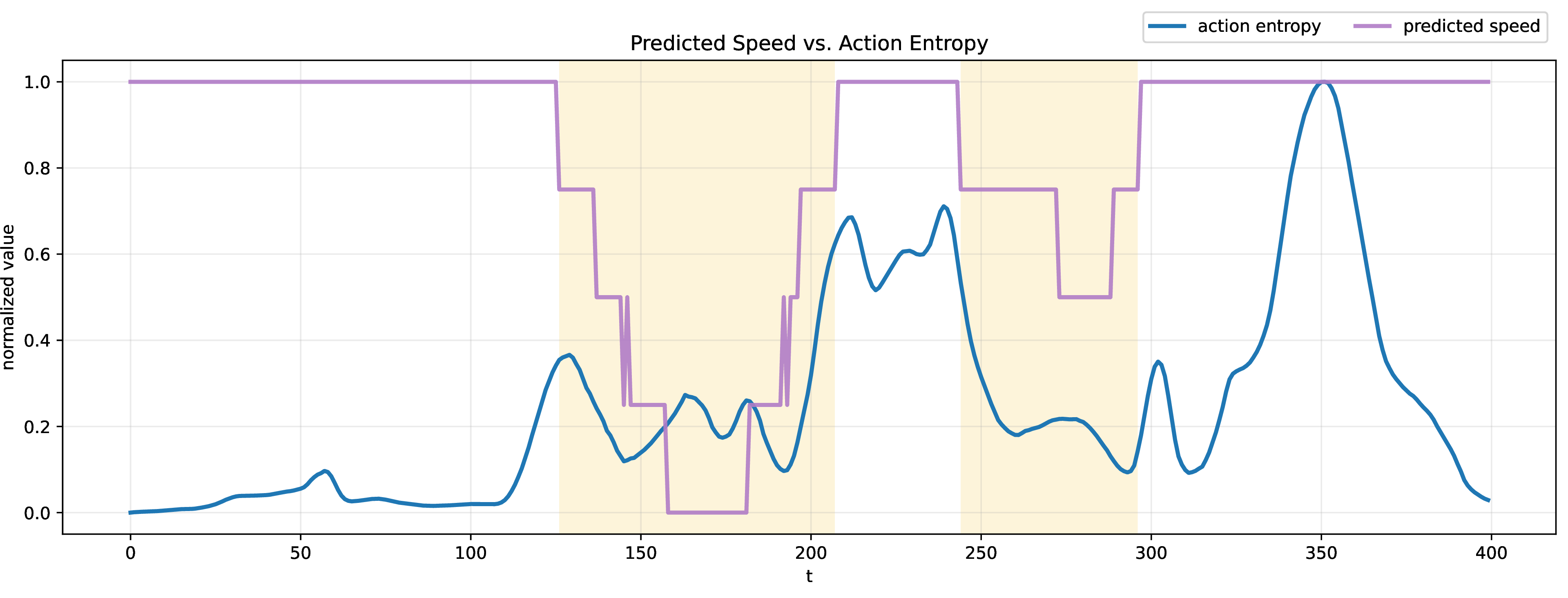
Beyond qualitative observations, we further analyze the consistency between the predicted speed ratios and action entropy from DemoSpeedUp (Ref. [11] in the main paper), which reflects divergence across multiple sampled action predictions. As shown in 9, their extrema are stage-aligned: lower predicted speeds correspond to higher action-entropy stages. Unlike action entropy, which relies on grouped predictions from a proxy policy and struggles to distinguish uncertainty from multi-modality, AutoSpeed more accurately identifies safely acceleratable stages, such as robot start-up and return-to-home fast motions.
11 More AutoSpeed-Identified Speed Ratio Curves↩︎

11.1 Qualitative Analysis in Simulation Tasks↩︎
In this section, we present a qualitative analysis of the motion speed trajectories predicted by the AutoSpeed framework across diverse simulation environments. As illustrated in Figure 10, the inferred speed ratios exhibit a strong, interpretable correspondence with the underlying task phases without any explicit annotations.
In the Transfer Cube task from the ALOHA benchmark [1], the robot must perform a bimanual object handover, transferring a cube from the right gripper to the left. The predicted speed curve accurately captures the two most interaction-critical phases. The policy first decelerates significantly to approach and grasp the cube with the right arm. Following a brief period of high-speed transit, the speed drops to its minimum during the complex object handover, where precise coordination is required as the left arm approaches and grasps the cube, and the right arm releases. Other phases are executed efficiently at higher speeds.
The long-horizon task from LIBERO-10 [30] (Turn on the Stove and Put the Moka Pot on It) involves three sequential interaction stages. The speed curve accurately reflects this multi-stage complexity by exhibiting three corresponding deceleration valleys. Specifically, AutoSpeed actively drops the execution speed when the gripper makes contact with the stove knob, when it carefully grasps the handle of the moka pot, and when it precisely aligns the pot onto the stove burner. The coarse reaching motions bridging these interaction phases are executed efficiently at peak speeds.
The Meta-World [31] task demands the policy to Pick up a Nut and Place It onto A Peg. Firstly the arm approaches the nut quickly, slows down to grasp, and accelerates moderately during transport. Notably, during the most challenging stage where the arm should hover and align the nut with the peg, the policy executes at its minimum speed to improve spatial precision. Finally, once the nut is successfully placed, the arm swiftly retracts.
11.2 More Curves↩︎
This is an interesting dynamic manipulation task named Mole Game, where an xArm 7 must press a randomly lit button within 2 s. This task provides an intuitive demonstration of AutoSpeed’s characteristics. We visualize the learned ratio curve after training in Fig. 11. In safe motion phases, the policy increases the motion speed, while in critical interaction phases, such as button pressing, it slows down to ensure precise execution.