Generative Model Proposal based Particle Filtering for Data Assimilation
July 01, 2026
Abstract
Data assimilation models state dynamics conditioned on sequential observations, and has wide-ranging scientific applications. In the filtering setting, the goal is to model the posterior over the current state given all observations so far. Classical solutions typically make simplifying distributional or functional assumptions, e.g., linear-Gaussian systems, which can be inaccurate in many scenarios. In principle, particle filters (PFs) remove these assumptions, yet often collapse in high dimensions. Recent generative approaches learn conditional state transitions, but without principled Bayesian updates they do not recover the correct filtering posterior and can accumulate error over long horizons. In this work, we introduce Flow Proposal Particle Filters (FPPF), which learn a conditional generative model based proposal approximating the variance-minimizing optimal proposal for particle propagation. Conditioning on observations steers particles toward high-likelihood regions before weighting, reducing weight variance and delaying degeneracy. Since our proposal admits tractable likelihood evaluation, FPPF computes accurate importance weights and retains a Bayesian update step. We further extend FPPF to high-dimensional problems through localization strategies, adressing another standard PF failure mode. Extensive experiments on a variety of dynamical systems show that FPPF outperforms statistical baselines and other generative methods in non-linear, non-Gaussian, and high-dimensional regimes. Code is available at https://github.com/cnagda/fppf/tree/main.
1 Introduction↩︎
Data assimilation (DA) is the inverse problem of inferring the latent state trajectory \(\mathbf{x}_{1:T}\) of a dynamical system from imperfect observations \(\mathbf{o}_{1:T}\), using knowledge of the system’s dynamics \(p(\mathbf{x}_t \mid \mathbf{x}_{t-1})\) and an observation model \(p(\mathbf{o}_t \mid \mathbf{x}_t)\). DA is fundamental to many scientific and engineering applications, including weather forecasting [1]–[3], climate analysis [4], [5], agriculture [6], [7], and motion tracking [8], [9]. In these domains, point estimates of latent states \(\mathbf{x}_t\) alone are inadequate. Since downstream decisions based on latent state estimates carry significant consequences, reliable uncertainty quantification requires recovering a full distribution over states.
In this work, we focus on one of the most widely studied DA tasks called filtering [10], [11]: at time \(t\), given observations \(\mathbf{o}_{1:t}\), we seek the filtering posterior \(p(\mathbf{x}_t \mid \mathbf{o}_{1:t})\). Bayesian filtering proceeds via a recursive prediction–update cycle, in which the state dynamics model defines the prior over the next state, and conditioning on the observation using Bayes’ rule gives the posterior. When the dynamics and observation models are linear and the noise is Gaussian, this is solved exactly by the Kalman filter (KF) [12]. To handle nonlinear dynamics, models like the Ensemble KF (EnKF) [13], which are heavily used in operational settings [14], propagate an ensemble of samples through the true dynamics but retain Gaussian assumptions in the update step.
In principle, particle filters (PFs) [15], [16] provide an appealing alternative, performing Bayesian filtering without linearity or Gaussianity assumptions by representing the posterior through a weighted ensemble of particles. However, they suffer from degeneracy: in high-dimensional state spaces, the ensemble size required to prevent the weights from collapsing onto a few particles grows exponentially with the effective state dimension [17], [18]. Intuitively, particles propagated through the dynamics model often do not land in regions supported by the new observations, so most receive negligible weight. This curse of dimensionality has largely confined particle filters to low-dimensional problems.
In the general sequential importance resampling (SIR) framework [19], one samples from an arbitrary proposal \(q(\mathbf{x}_t \mid \mathbf{x}_{t-1}, \mathbf{o}_t)\) and corrects via importance weights. The variance-minimizing choice is the optimal proposal \(q^\star(\mathbf{x}_t \mid \mathbf{x}_{t-1}, \mathbf{o}_t) = p(\mathbf{x}_t \mid \mathbf{x}_{t-1}, \mathbf{o}_t)\), which steers particles toward regions supported by the new observation before weighting [16]. However, \(q^\star\) is hard to compute outside special cases (such as linear-Gaussian models) which reintroduce restrictive assumptions. A line of work has sought to move beyond this setting by incorporating the incoming observation into how particles are selected or propagated, including look-ahead particle selection [20], implicit sampling via per-particle optimization [21], [22], and equal-weight constructions [23], [24]. However, these schemes either recover \(q^\star\) only under restrictive distributional structure or replace it with a hand-designed surrogate, limiting their fidelity in the nonlinear, non-Gaussian regimes that motivate PFs in the first place. What we would want instead is a flexible approximation to \(q^\star\) that keeps the full generality of PFs.
This is where recent ML-based approaches to DA become relevant. Recent methods [25], [26] learn the conditional \(p(\mathbf{x}_t \mid \mathbf{x}_{t-1}, \mathbf{o}_t)\) directly with a generative model; note that this is precisely the object the optimal proposal requires, free of Gaussian or linearity assumptions. The prevailing strategy, however, is to apply the learned conditional autoregressively, rolling a state estimate forward by repeatedly sampling from the generator. This amounts to propagating a single unweighted particle: at no point is the filtering posterior \(p(\mathbf{x}_t \mid \mathbf{o}_{1:t})\) formed by combining the propagated prior \(p(\mathbf{x}_t \mid \mathbf{o}_{1:t-1})\) with the likelihood \(p(\mathbf{o}_t \mid \mathbf{x}_t)\) via Bayes’ rule. Thus, each step incurs a discrepancy with respect to the filtering posterior and empirically, these purely generative rollouts rapidly accumulate error over long horizons.
In this work, we show that these two threads resolve each other. SIR filters benefit from a flexible approximation of \(q^\star\); generative DA methods learn one, but deploy it naively. We propose Flow Proposal Particle Filters (FPPF), which uses a learned conditional distribution as a proposal. Particles are proposed in an observation-informed manner and then reweighted, so the filter targets the true posterior even when the proposal is imperfect, while proximity to \(q^\star\) keeps weight variance low and delays degeneracy. While natural in hindsight, realizing this step is nontrivial. We show how to learn \(q_\phi(\mathbf{x}_t \mid \mathbf{x}_{t-1}, \mathbf{o}_t)\) with conditional flow matching, which offers both efficient sampling and exact likelihood evaluation via the instantaneous change-of-variables formula, making the weight computation feasible. To extend the approach to high-dimensional settings, where even well-proposed particles suffer weight collapse, we introduce a localized variant, L-FPPF, whose velocity network yields a per-site factorization of the proposal log-density and keeps both computation and weighting local.
We evaluate FPPF and L-FPPF on chaotic dynamical systems, including Lorenz-63, Lorenz-96, and the Kuramoto-Sivashinsky equation, under both Gaussian and strongly non-Gaussian observation operators, against classical filters, prior proposal learning methods, autoregressive generative DA, and localized particle filters. FPPF consistently improves state estimation accuracy and probabilistic calibration over these baselines, with the largest gains in non-Gaussian regimes where Kalman updates fail. Unlike autoregressive rollouts, it remains stable over long assimilation horizons. L-FPPF sustains these gains as the state dimension grows, whereas global PFs degenerate.
We summarize our main contributions below:
.
We propose FPPF, a filtering method that learns an observation-informed conditional generative model based proposal distribution approximating the variance-minimizing optimal proposal, and integrates it into the standard sequential importance resampling framework.
We instantiate the proposal with conditional flow matching, and show that likelihood evaluation can be leveraged to compute particle weights for a principled update step.
To extend the approach to high-dimensional settings, we propose L-FPPF, which uses a patch-based velocity network to obtain a factorization of the proposal log-density, extending localized particle filtering to general learned proposals.
We empirically demonstrate on chaotic dynamical systems (Lorenz-63, Lorenz-96, Kuramoto-Sivashinsky) that FPPF improves state estimation and probabilistic calibration over classical baselines and autoregressive generative models, and that L-FPPF scales to high-dimensional systems.
The rest of the paper is organized as follows. Section 2 reviews related work, Section 3 provides background on Bayesian filtering and particle filters, Sections 4 and 5 present FPPF and its localized variant L-FPPF, Section 6 reports experiments, and we conclude in Section 7.
2 Related Work↩︎
2.0.0.1 Classical data assimilation.
The Kalman filter solves linear-Gaussian filtering exactly [12]. The EnKF and its transform variants propagate an ensemble through nonlinear dynamics but retain a Gaussian update [13], [27], [28], and are widely used in operational weather prediction [29], [30]. Variational methods such as 3D-Var and 4D-Var optimize a cost over the state trajectory [31], [32], producing point estimates rather than the posterior distributions we target.
Particle filters drop these assumptions entirely [15], but the bootstrap proposal ignores the incoming observation, and the ensemble size needed to prevent weight collapse grows exponentially with the effective state dimension [18], [33]. The optimal proposal \(q^\star\) minimizes incremental weight variance [16] but is hard to obtain. Classical mitigations approximate it indirectly: APF selects ancestors by observation look-ahead without changing where particles land [20], implicit sampling targets posterior modes via per-particle optimization [21], [22], and equal-weight constructions hand-design moves toward the observation [23], [24]. These recover \(q^\star\) only under restrictive structure or replace it with a surrogate. For spatially extended systems, localized PFs attack degeneracy along a different axis, computing weights and resampling per region from tapered local likelihoods [34]–[36]. This construction is specific to the bootstrap PF, whose weight is just the local observation likelihood; L-FPPF extends localization to learned proposals.
2.0.0.2 Learned proposals for SMC.
Early adaptive methods optimize proposals within parametric families with closed-form densities [37], [38]. NASMC [39] and variational SMC [40]–[42] learn neural proposals by running a particle filter inside the training loop, yielding gradient estimates that suffer high variance when the proposal is poor or due to resampling. InfNN [43] trains offline by maximum likelihood but restricts the proposal to a factorized autoregressive form to keep its density tractable. In contrast, FPPF trains offline by velocity regression on simulated tuples, imposes no distributional form, and retains exact density evaluation via the instantaneous change-of-variables formula.
2.0.0.3 Generative models for data assimilation.
Score- and flow-based generative models have been applied to DA in two ways. The first learns a conditional generator for the states themselves, incorporating observations through inference-time methods such as guidance or inpainting: SDA samples short trajectory windows given observations [44], while DiffDA and FlowDAS apply a one-step conditional generator autoregressively [25], [26]. The guided iterates are not draws from the filtering posterior, and in the autoregressive case this discrepancy compounds, so errors accumulate over long rollouts (Section 6.3). A second line of work targets the analysis distribution: EnSF [45] and EnFF [46] estimate the score or velocity of the filtering density training-free and fold in observations through likelihood-gradient guidance, latent variants improve handling of sparse observations [47], [48], and the concurrent DAISI folds forecast information into a pretrained prior by inverse sampling before guidance [49]. In both approaches observations enter through guidance, an approximate correction to the generative dynamics, with no mechanism to remove the resulting bias. Closest and concurrent to our work, [50] restore the Bayesian update for this class, guiding a pretrained diffusion emulator with the likelihood score inside a fully adapted auxiliary PF; FPPF learns a directly conditioned proposal whose tractable density supplies the full SIR correction, keeping the update valid even when the proposal is imperfect.
2.0.0.4 Learning the state-space model components.
A complementary thread learns components of the state-space model itself. [51] emulate dynamics from EnKF analyses, [52] jointly infer the dynamical model and the state, and AD-EnKF [53] differentiates through the EnKF for joint state and parameter estimation. Differentiable particle filters likewise learn transition, observation, and proposal end-to-end through differentiable resampling [54]–[58]. These methods target model learning and parameter estimation; we assume known dynamics and observation models and learn only the proposal, which also avoids optimizing through the filter over long chaotic trajectories.
3 Background and Preliminaries↩︎
This section reviews the Bayesian filtering approach to data assimilation, and provides background on particle filters and the proposal distribution.
3.1 Data Assimilation↩︎
We consider a dynamical system with latent state \(\mathbf{x}_t \in \mathbb{R}^{d_x}\) and observations \(\mathbf{o}_t \in \mathbb{R}^{d_o}\), where \(t\) denotes the discrete time index. The evolution of the system is governed by a state transition model \(p(\mathbf{x}_t \mid \mathbf{x}_{t-1})\). At each time step, observations are related to the latent state through the likelihood \(p(\mathbf{o}_t \vert \mathbf{x}_t)\). The goal is to estimate the filtering posterior \(p(\mathbf{x}_t \mid \mathbf{o}_{1:t})\), the distribution over the current state given all observations up to time \(t\). In the Bayesian filtering framework [10], [19], [59], [60], this distribution is computed recursively via a prediction-update cycle: \[\label{eq:filtering} \begin{align} &p(\mathbf{x}_t \mid \mathbf{o}_{1:t-1}) = \int p(\mathbf{x}_t \mid \mathbf{x}_{t-1}) p(\mathbf{x}_{t-1} \mid \mathbf{o}_{1:t-1}) \, d\mathbf{x}_{t-1}~, && \textcolor{predictcol}{\boldsymbol{[\mathrm{\small Predict}]}} \\ &p(\mathbf{x}_t \mid \mathbf{o}_{1:t}) \propto p(\mathbf{o}_t \mid \mathbf{x}_t) p(\mathbf{x}_t \mid \mathbf{o}_{1:t-1})~. && \textcolor{updatecol}{\boldsymbol{[\mathrm{\small Update}]}} \end{align}\tag{1}\] For linear-Gaussian systems, i.e.when the transition dynamics are linear and the observation likelihood is Gaussian, the Kalman filter (KF) [12] provides an analytical solution to this recursion. Nonlinear extensions relax these assumptions approximately: the extended KF linearizes the dynamics and observation models [59], the unscented KF propagates deterministically chosen sigma points [61], and the ensemble KF [13] replaces analytical covariance propagation with an ensemble, but retains a Gaussian update. In general, for nonlinear dynamics and non-Gaussian observation models, the prediction integral remains intractable and the update step admits no closed form, necessitating other inference methods.
3.2 Particle Filters↩︎
Particle filters (PFs) approximate the filtering posterior \(p(\mathbf{x}_t \mid \mathbf{o}_{1:t})\) using a weighted ensemble of \(N\) samples \(\{ \mathbf{x}_t^{(i)}, w_t^{(i)} \}_{i=1}^N\) with \(\sum_i w_t^{(i)} = 1\), representing the posterior through the empirical measure \(\sum_i w_t^{(i)} \delta_{\mathbf{x}_t^{(i)}}\).
3.2.0.1 Bootstrap particle filter.
The bootstrap particle filter (BPF) [15] instantiates the recursion of Eq. 1 via Monte Carlo. Given the weighted ensemble \(\{\mathbf{x}_{t-1}^{(i)}, w_{t-1}^{(i)}\}\) approximating \(p(\mathbf{x}_{t-1} \mid \mathbf{o}_{1:t-1})\), the Predict step propagates each particle through the transition dynamics, and the Update step reweights by the new observation likelihood: \[\label{eq:bpf} \begin{align} \mathbf{x}_t^{(i)} &\sim p(\mathbf{x}_t \mid \mathbf{x}_{t-1}^{(i)})~, && \textcolor{predictcol}{\boldsymbol{[\mathrm{\small Predict}]}} \\ w_t^{(i)} &\propto w_{t-1}^{(i)} \, p(\mathbf{o}_t \mid \mathbf{x}_t^{(i)})~, \qquad \textstyle\sum_i w_t^{(i)} = 1~. && \textcolor{updatecol}{\boldsymbol{[\mathrm{\small Update}]}} \end{align}\tag{2}\] Sampling from the transition realizes the prediction integral in Eq. 1 , and multiplying by the likelihood realizes the Bayesian update; the weight recursion is exactly importance sampling against the one-step prior. The BPF is appealing because it requires only the ability to simulate the dynamics and evaluate the likelihood, with no Gaussian or linearity assumptions.
3.2.0.2 Weight degeneracy.
The standard BPF suffers from degeneracy in high-dimensional spaces because particles propagated through the transition prior often fail to land in regions supported by the new observations. Consequently, most particles receive negligible weight, causing the mass to collapse onto a single particle during the Update step. The severity of this collapse is captured by the variance of the log-likelihoods across the propagated ensemble, \(\tau^2 := \mathrm{Var}\big[\log p(\mathbf{o}_t \mid \mathbf{x}_t^{(i)})\big]\): [18] and [17] show that the largest normalized weight tends to \(1\) unless the ensemble size satisfies \(\log N \gtrsim \tau^2/2\). Since \(\tau^2\) grows roughly linearly with the effective dimension of the system, avoiding degeneracy demands \(N \gtrsim \exp(\tau^2/2)\) particles, a requirement that quickly becomes intractable and fundamentally limits the use of BPF in high-dimensional domains [62].
3.2.0.3 Resampling.
To mitigate weight degeneracy, which occurs even in low-dimensional problems, the BPF resamples. This step draws \(N\) particles with replacement proportional to \(w_t^{(i)}\), duplicating high-weight particles, discarding low-weight ones, and resetting all weights to \(1/N\) [15], [63]. Stochastic model dynamics can subsequently restore particle diversity. However, if the weights collapse completely before resampling, the algorithm duplicates a single surviving particle \(N\) times, an unrecoverable loss of diversity known as sample impoverishment [64]. Therefore, keeping weights balanced is a fundamental problem, and designing better proposal distributions provides a path to achieving this.
3.2.0.4 Proposal distribution.
The sequential importance resampling (SIR) framework [16], [65] generalizes BPF by drawing particles from a proposal \(q(\mathbf{x}_t \mid \mathbf{x}_{t-1}, \mathbf{o}_t)\) that may depend on the current observation, with weights updated as \[\label{eq:sir95weight} w_t^{(i)} \propto w_{t-1}^{(i)} \, \frac{p(\mathbf{o}_t \mid \mathbf{x}_t^{(i)}) \, p(\mathbf{x}_t^{(i)} \mid \mathbf{x}_{t-1}^{(i)})}{q(\mathbf{x}_t^{(i)} \mid \mathbf{x}_{t-1}^{(i)}, \mathbf{o}_t)} \, .\tag{3}\] BPF corresponds to the choice \(q = p(\mathbf{x}_t \mid \mathbf{x}_{t-1})\), which ignores \(\mathbf{o}_t\) at the Predict stage; the incremental weight then reduces to the likelihood \(p(\mathbf{o}_t \mid \mathbf{x}_t^{(i)})\) (Eq. 2 ). A natural way to do better is to fold the current observation into the proposal itself, drawing from \(p(\mathbf{x}_t \mid \mathbf{x}_{t-1}, \mathbf{o}_t)\). Expanding this density by Bayes’ rule, and using that \(\mathbf{o}_t\) depends on the state only through \(\mathbf{x}_t\) so that \(p(\mathbf{o}_t \mid \mathbf{x}_t, \mathbf{x}_{t-1}) = p(\mathbf{o}_t \mid \mathbf{x}_t)\), gives \[\label{eq:optimal95proposal} q^\star(\mathbf{x}_t \mid \mathbf{x}_{t-1}, \mathbf{o}_t) = p(\mathbf{x}_t \mid \mathbf{x}_{t-1}, \mathbf{o}_t) = \frac{p(\mathbf{o}_t \mid \mathbf{x}_t, \mathbf{x}_{t-1}) \, p(\mathbf{x}_t \mid \mathbf{x}_{t-1})}{p(\mathbf{o}_t \mid \mathbf{x}_{t-1})} = \frac{p(\mathbf{o}_t \mid \mathbf{x}_t) \, p(\mathbf{x}_t \mid \mathbf{x}_{t-1})}{p(\mathbf{o}_t \mid \mathbf{x}_{t-1})} \, .\tag{4}\] Substituting \(q^\star\) into the weight update collapses the numerator against the proposal, leaving \[\label{eq:opt-weight} w_t^{(i)} \propto w_{t-1}^{(i)} \, p(\mathbf{o}_t \mid \mathbf{x}_{t-1}^{(i)}) \, ,\tag{5}\] so that the weight at time \(t\) depends only on the ancestor particle \(\mathbf{x}_{t-1}^{(i)}\) and not on the sampled \(\mathbf{x}_t^{(i)}\). In this sense, the proposal \(q^\star\) is often termed “optimal” [16]: conditional on \(\mathbf{x}_{t-1}^{(i)}\) and \(\mathbf{o}_t\), the incremental weight is independent of the random draw \(\mathbf{x}_t^{(i)}\), and hence has zero variance with respect to the proposal. This optimality is therefore local; it does not imply that the resulting particle filter performs optimally overall, but only that it minimizes the variance \(\mathrm{Var}\!\big(w_t^{(i)}/w_{t-1}^{(i)} \mid \mathbf{x}_{t-1}^{(i)}, \mathbf{o}_t\big)\) introduced at the current sampling step. Intuitively, this proposal shifts the effect of the likelihood from the weighting step into the sampling step, so that particles are drawn preferentially in regions of high posterior probability, which reduces the weight degeneracy problem, although it does not completely solve it.
3.2.0.5 High-dimensional particle filtering.
The optimal proposal above admits a tractable closed form only in special cases, most notably linear–Gaussian state space models, where \(q^\star\) is Gaussian and reproduces the Kalman analysis [16]. Outside these restricted settings, evaluating the normalizing integral in \(p(\mathbf{o}_t \mid \mathbf{x}_{t-1})\) is intractable, and even if one can sample exactly from \(q^\star\), the ensemble size required to avoid weight collapse still grows too rapidly for many high-dimensional problems [17], [18], [62].
A wide range of approaches has been proposed to mitigate this degeneracy [66]. One primary direction builds more informative proposals that fold the observation into propagation, but approximates \(q^\star\) only indirectly. The auxiliary particle filter (APF), for instance, performs a one-step look-ahead through a first-stage weight \[\lambda_t^{(i)} \propto w_{t-1}^{(i)} \, p\big(\mathbf{o}_t \mid \boldsymbol{\mu}_t^{(i)}\big), \qquad \boldsymbol{\mu}_t^{(i)} = \mathbb{E}\big[\mathbf{x}_t \mid \mathbf{x}_{t-1}^{(i)}\big],\] that ranks ancestors by the observation likelihood at their predicted mean without changing where particles are drawn. Other approaches such as implicit sampling and equal-weight constructions (Section 2), also recover \(q^\star\) only under restrictive distributional structure.
A second primary direction exploits spatial locality. Localized particle filters partition the domain into regions \(\{\mathcal{B}_b\}\) with centers \(c_b\) and weight each from a tapered local likelihood, \[\log w_{b,t}^{(i)} \propto \log w_{t-1}^{(i)} + \sum_{o} G\!\left(\frac{d(o, c_b)}{r_{\mathrm{loc}}}\right) \log p\big(\mathbf{o}_{t,o} \mid \mathbf{x}_t^{(i)}\big),\] so that a region’s effective dimension is governed by the radius \(r_{\mathrm{loc}}\) rather than \(d_x\) [34], [67]. This localization, however, is formulated for the bootstrap proposal, whose weight is simply the observation likelihood.
Our method builds on both threads, learning an approximation of \(q^\star\) with a tractable weight correction and extending it to a localized setting for high-dimensional problems.
4 Flow Proposal Particle Filter (FPPF)↩︎
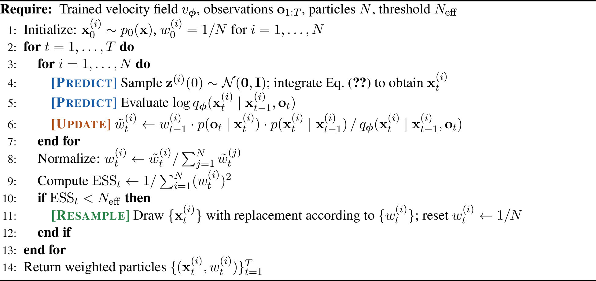
We now present Flow Proposal Particle Filter (FPPF), our approach for learning proposal distributions that approximate the locally optimal proposal. We parameterize the proposal using conditional flow matching (FM) [68], [69], a generative modeling framework that learns a time-dependent velocity field to transport samples from a simple base distribution to a target distribution via an ordinary differential equation (ODE). FM admits stable and efficient training via simple regression and tractable exact density evaluation for importance weight computation. The full method is summarized in Algorithm 1.
4.1 Learning the Proposal Distribution↩︎
We learn a conditional proposal distribution for the filtering problem of the form \(q_\phi(\mathbf{x}_t \mid \mathbf{x}_{t-1}, \mathbf{o}_t)\), used to propagate particles from time \(t-1\) to time \(t\) given the current observation. It is a flexible approximation to the locally optimal proposal \(q^\star(\mathbf{x}_t \mid \mathbf{x}_{t-1}, \mathbf{o}_t)\) of Eq. 4 . The proposal is parameterized implicitly via a conditional velocity field \(v_\phi(\mathbf{z}(s), s; \mathbf{x}_{t-1}, \mathbf{o}_t)\) that defines a deterministic flow transporting samples from a simple base distribution to the proposal distribution.
Here \(t\) is the discrete filtering time indexing the state sequence, while \(s \in [0,1]\) is an auxiliary flow time internal to the generative model; one full integration in \(s\) produces a single proposal draw at filtering step \(t\). We define \(\mathbf{z}(s)\) by the ordinary differential equation, holding the conditioning variables \((\mathbf{x}_{t-1}, \mathbf{o}_t)\) fixed: \[\frac{d\mathbf{z}(s)}{ds} = v_\phi\!\left(\mathbf{z}(s), s; \mathbf{x}_{t-1}, \mathbf{o}_t \right), \qquad \mathbf{z}(0) \sim \mathcal{N}(\mathbf{0}, \mathbf{I}). \label{eq:proposal95ode}\tag{6}\] Integrating 6 from \(s=0\) to \(s=1\) yields a proposal sample \(\mathbf{x}_t := \mathbf{z}(1)\).
4.1.0.1 Network conditioning.
We parameterize \(v_\phi\) as a neural network taking as input both the previous state \(\mathbf{x}_{t-1}\) and the current observation \(\mathbf{o}_t\) to approximate the optimal proposal. We use simple concatenation, providing \([\mathbf{x}_{t-1}; \mathbf{o}_t]\) as additional input alongside the noised state \(\mathbf{x}_s\) and flow time \(s\). Alternative conditioning mechanisms such as FiLM [70] or cross-attention can also be employed. We choose direct conditioning, rather than guidance-based approaches [25], [71] that incorporate observations at inference time by adding an approximate likelihood-gradient term to the generative drift. Inference-time guidance is appealing because the same generative prior serves any observation model without retraining; however, in practice the guidance scale is sensitive to the observation operator and noise level and must be retuned per setting (too small and the observation is under-enforced, too large and the approximate gradient distorts the samples) [72], [73]. It also keeps density evaluation simple: with no auxiliary likelihood-gradient term in the dynamics, the proposal density follows from applying the change-of-variables formula to \(v_\phi\) alone (Section 4.2).
To prevent the model from over-relying on observations, which could degrade performance when they are noisy or uninformative, we apply observation dropout during training (similar to [72]): for each training tuple independently, with probability \(p_{\mathrm{cond}}\) we replace the entire observation vector \(\mathbf{o}_t\) with zeros, while leaving \(\mathbf{x}_{t-1}\) intact. This exposes the network to both observation-conditioned and observation-free inputs, encouraging it to also leverage dynamical information from \(\mathbf{x}_{t-1}\) rather than relying solely on \(\mathbf{o}_t\). We use \(p_{\mathrm{cond}} = 0.1\). Similarly, to prevent over-reliance on the previous state \(\mathbf{x}_{t-1}\), we corrupt it during training with a coordinate-masking schedule. At training step \(k\) of \(K\) total, with probability \(p_{\mathrm{mask}}(k) = \max\!\big(p_{\min},\, p_0(1 - k/K)\big)\) we zero a uniformly random subset of \(\lceil r_{\mathrm{mask}}\, d_x \rceil\) coordinates of \(\mathbf{x}_{t-1}\) before passing it to the network, and otherwise use it intact. The masking probability is annealed linearly from \(p_0\) to a floor \(p_{\min}\) over training, so the network is forced to recover masked coordinates from \(\mathbf{o}_t\) early on, when it would otherwise lock onto the highly predictable dynamics, and is relaxed toward the clean state as training converges. All masking is disabled at inference.
4.1.0.2 Training data.
For a given dynamical system, using a transition model \(p(\mathbf{x}_t \mid \mathbf{x}_{t-1})\) and an observation model \(p(\mathbf{o}_t \mid \mathbf{x}_t)\), we simulate trajectories and form supervised training tuples \((\mathbf{x}_{t-1}, \mathbf{o}_t, \mathbf{x}_t)\), where \(\mathbf{o}_t\) is sampled from \(p(\mathbf{o}_t \mid \mathbf{x}_t)\). Specific choices for trajectory generation are in Section 6.
4.1.0.3 Conditional flow matching objective.
Following [69], we adopt linear interpolation paths between paired base and target samples, which induce a target velocity \(\mathbf{z}(1) - \mathbf{z}(0)\) that \(v_{\boldsymbol{\phi}}\) regresses onto. For each training tuple, we sample noise \(\mathbf{z}(0) \sim \mathcal{N}(\mathbf{0}, \mathbf{I})\), set \(\mathbf{z}(1) := \mathbf{x}_t\), draw \(s \sim \mathrm{Unif}[0,1]\), and form the linear interpolant \(\mathbf{z}(s) = (1-s)\mathbf{z}(0) + s\mathbf{z}(1)\), whose constant velocity is \(\mathbf{z}(1) - \mathbf{z}(0)\). We train \(v_{\boldsymbol{\phi}}\) to regress onto this target by minimizing \[\mathcal{L}_{\mathrm{FM}}({\boldsymbol{\phi}}) = \mathbb{E}_{(\mathbf{x}_{t-1}, \mathbf{o}_t, \mathbf{x}_t),\, \mathbf{z}(0),\, s} \left[ \big\| v_{\boldsymbol{\phi}}\big(\mathbf{z}(s), s;\, \mathbf{x}_{t-1}, \mathbf{o}_t\big) - \big(\mathbf{z}(1) - \mathbf{z}(0)\big) \big\|_2^2 \right], \label{eq:fm95objective}\tag{7}\] where \((\mathbf{x}_{t-1}, \mathbf{o}_t, \mathbf{x}_t)\) is a training tuple from the simulated trajectories (with \(\mathbf{z}(1) := \mathbf{x}_t\)), \(\mathbf{z}(0) \sim \mathcal{N}(\mathbf{0}, \mathbf{I})\), \(s \sim \mathrm{Unif}[0,1]\), and \(\mathbf{z}(s) = (1-s)\mathbf{z}(0) + s\,\mathbf{z}(1)\).
4.2 Importance Weight Computation↩︎
Given particles \(\{(\mathbf{x}_{t-1}^{(i)}, w_{t-1}^{(i)})\}_{i=1}^N\) approximating \(p(\mathbf{x}_{t-1} \mid \mathbf{o}_{1:t-1})\) (weights initialized to \(1/N\)), we sample \(\mathbf{x}_t^{(i)} \sim q_{\boldsymbol{\phi}}(\mathbf{x}_t \mid \mathbf{x}_{t-1}^{(i)}, \mathbf{o}_t)\) via 6 . We then apply the SIR update of Eq. 3 with our learned proposal \(q_{\boldsymbol{\phi}}\) (Algorithm 1, line 7): \[\tilde{w}_t^{(i)} = w_{t-1}^{(i)} \frac{p(\mathbf{o}_t \mid \mathbf{x}_t^{(i)}) \, p(\mathbf{x}_t^{(i)} \mid \mathbf{x}_{t-1}^{(i)})}{q_{\boldsymbol{\phi}}(\mathbf{x}_t^{(i)} \mid \mathbf{x}_{t-1}^{(i)}, \mathbf{o}_t)}. \label{eq:weight95update}\tag{8}\] Since the model dynamics and observation model are known, the numerator is straightforward to compute. A key property of FM is exact density evaluation via the instantaneous change of variables formula [74]. For a sample \(\mathbf{x}_t\) generated by integrating Eq. 6 from initial noise \(\mathbf{z}(0)\), \[\log q_{\boldsymbol{\phi}}(\mathbf{x}_t \mid \mathbf{x}_{t-1}, \mathbf{o}_t) = \log p_0(\mathbf{z}(0)) - \int_0^1 \mathrm{Tr}\left(\frac{\partial v_{\boldsymbol{\phi}}}{\partial \mathbf{z}(s)}\right) ds,\] where \(p_0 = \mathcal{N}(\mathbf{0}, \mathbf{I})\) is the base distribution. Computing the exact trace requires \(d_x\) backward passes through the network, which becomes prohibitive in high dimensions. We instead use the Hutchinson trace estimator, as in previous works [74]: \(\mathrm{Tr}(\mathbf{J}) = \mathbb{E}_{\boldsymbol{\epsilon}}\left[\boldsymbol{\epsilon}^\top \mathbf{J} \boldsymbol{\epsilon}\right],\) where \(\boldsymbol{\epsilon}\) satisfies \(\mathbb{E}[\boldsymbol{\epsilon}\mathbf{\epsilon}^\top] = \mathbf{I}\). The vector-Jacobian product \(\boldsymbol{\epsilon}^\top \mathbf{J}\) is computed efficiently via a single backward pass. We use Rademacher random vectors (\(\epsilon_j \in \{-1, +1\}\) uniformly). For a fixed matrix \(\mathbf{J}\), the single-probe estimator variance is \(2\|\mathbf{J}\|_F^2\) for Gaussian probes and \(2\sum_{i \neq j} J_{ij}^2\) for Rademacher probes [75]; the latter removes the diagonal contribution and is never larger, which is why Rademacher probes are standard and match our empirical observation of lower variance. Finally, resampling is triggered when the effective sample size \(\mathrm{ESS} = 1 / \sum_i (w_t^{(i)})^2\) falls below a threshold \(N_{\mathrm{eff}}\) [63].
4.2.0.1 Temporally sparse observations.
When no observation is available at a given step, we default to the bootstrap transition, sampling \(\mathbf{x}_t^{(i)} \sim p(\mathbf{x}_t \mid \mathbf{x}_{t-1}^{(i)})\) and omitting the observation update, and apply the learned proposal and SIR correction only at steps where an observation arrives.
5 Localized Flow Proposal Particle Filter (L-FPPF)↩︎
Particle filters require ensembles that grow exponentially with the effective state dimension (Section 3.2), even under the optimal proposal [33], [62]. One solution is localization, which mitigates this by exploiting sparse conditional dependence. Such structure is naturally described by a graphical model, i.e. the filtering posterior factorizes according to a graph whose nodes are the state coordinates (which we call sites) and whose edges encode direct statistical dependence, so that each site is conditionally independent of the rest given its neighbors [76]. Sparse graphs of this kind are common in high-dimensional dynamical systems and can be learned from data when not known a priori [77], [78]. In the spatially extended systems we study the graph is both known and local, since each site couples directly only to its spatial neighbors.
5.0.0.1 Localized Particle Filters (LPFs).
A class of methods known as localized particle filters (LPFs) exploit this structure to avoid collapse [34]–[36]. Exact inference over a graphical model is tractable only when the graph has small treewidth, a condition the dense couplings of a filtering posterior generally violate, so localized PFs approximate the single global update with many overlapping local ones. Each local update is restricted by a localization radius, which bounds its effective dimension independently of \(d_x\). Because the required ensemble size scales only with this local effective dimension, localization prevents weight collapse and drastically reduces the necessary number of particles for a high-dimensional problem. This whole construction rests on the bootstrap proposal. Because the bootstrap importance weight is just the observation likelihood \(p(\mathbf{o}_t \mid \mathbf{x}_t^{(i)})\) (Eq. 2 ), it factorizes over sites whenever the observation noise is independent across coordinates, and the per-site terms can then be tapered by spatial distance and aggregated block by block.
A learned proposal breaks this decomposition. We avoid the bootstrap proposal in the first place because it ignores the incoming observation and degenerates quickly in high dimensions, but moving to a learned \(q_\phi\) creates a different obstacle. A global velocity network couples all sites at once, so the proposal density \(\log q_\phi\) that appears in the denominator of the importance weight (Eq. 3 ) no longer factorizes, and without that factorization the weights cannot be localized. We therefore localize the proposal itself, restricting the network so that \(\log q_\phi\) factorizes across sites by construction.
5.0.0.2 Localized velocity field.
We replace the global velocity network with a patch network \(u_\phi\) shared across all state dimensions, which we call sites. For the spatially extended systems considered here, the sites lie on a periodic one-dimensional lattice, so neighborhoods wrap around at the boundary. Thus, the radius-\(r\) neighborhood of site \(j\) is \(W_j^r=\{j-r,\ldots,j+r\}\), where indices outside \(\{1,\ldots,d_x\}\) are wrapped periodically. Writing \(c_t=(\mathbf{x}_{t-1},\mathbf{o}_t)\), the localized velocity is \[v_{\phi,j}(\mathbf{z}(s),s;c_t) = u_\phi\!\left(\mathbf{z}_{W_j^r}(s),\mathbf{x}_{t-1,W_j^r},\mathbf{o}_{t,W_j^r},s\right). \label{eq:local95velocity}\tag{9}\]
This architecture is motivated by localized generative modeling. For distributions with sparse or approximately sparse graphical dependence, [79] show that score components can be approximated from local graph neighborhoods, with localization error decaying as the neighborhood radius grows. Their analysis applies to score-based diffusion models, while our proposal is trained by conditional flow matching along rectified-flow interpolation paths; we therefore use this result as motivation for imposing locality on the proposal velocity, leaving a formal analysis of localized rectified-flow proposals to future work. In the spatial systems considered here, the transition and observation mechanisms are local or coordinate-wise, so the observation-informed proposal \(q^\star(\mathbf{x}_t\mid\mathbf{x}_{t-1},\mathbf{o}_t)\) is expected to be dominated by local dependencies.
The locality constraint also makes proposal-density evaluation tractable. Since \(v_{\phi,j}\) depends only on \(\mathbf{z}_{W_j^r}\), the velocity Jacobian is sparse: \(\partial v_{\phi,j}/\partial z_k=0\) whenever \(k\notin W_j^r\). Applying the instantaneous change-of-variables formula used for the global FPPF proposal, the localized proposal log-density decomposes as \[\log q_\phi(\mathbf{x}_t\mid\mathbf{x}_{t-1},\mathbf{o}_t) = \sum_{j=1}^{d_x}\ell_j, \qquad \ell_j = \log \mathcal{N}(z_j(0);0,1) - \int_0^1 \frac{\partial v_{\phi,j}}{\partial z_j}(\mathbf{z}(s),s;c_t)\,ds . \label{eq:logq95local95trace}\tag{10}\] This follows because the base distribution factorizes across coordinates and the change-of-variables trace is the sum of diagonal Jacobian entries. The site-wise terms \(\ell_j\) provide the proposal-density contribution used by the localized SIR correction: in the block-wise update, each block \(B_b\) uses \(\sum_{j\in B_b}\ell_j\), together with the corresponding local transition and tapered observation-likelihood terms.
In implementation, local patches for all sites are formed as a single batch, and \(u_\phi\) is applied once to produce all site velocities in parallel. The diagonal terms \(\partial v_{\phi,j}/\partial z_j\) are computed exactly by differentiating each scalar site output with respect to the center coordinate of its input patch. Thus, L-FPPF replaces the Hutchinson trace estimator used by global FPPF with an exact deterministic trace computation whose cost scales with the local patch size. Training and implementation details are provided in Appendix 8.2.
5.0.0.3 Block-wise update step.
Following the standard LPF recipe [34], [36], we partition the state sites into \(B\) disjoint contiguous blocks \(\{\mathcal{B}_b\}_{b=1}^B\) with centers \(c_b\). The blocks determine where resampling decisions are made, and are distinct from the observation neighborhoods used to form the weights. Each block’s weight uses observations within a smooth distance-based taper around \(c_b\), so the neighborhoods of nearby blocks overlap even though the blocks themselves do not.
We obtain the block weights by localizing the global SIR log-weight (Eq. 8 ). We assume that the observation likelihood and the transition density to factorize over sites: \[\log p(\mathbf{o}_t \mid \mathbf{x}_t) = \sum_{m=1}^{d_o} \log p(o_{t,m} \mid \mathbf{x}_t), \qquad \log p(\mathbf{x}_t \mid \mathbf{x}_{t-1}) = \sum_{j=1}^{d_x} \log p(x_{t,j} \mid \mathbf{x}_{t-1}). \label{eq:factorization}\tag{11}\] This further requires that the observation and process noise are independent across coordinates (diagonal Gaussian noise in our experiments). Together with the per-site proposal terms \(\ell_j\) from Eq. 10 , every ingredient of the SIR correction is then site-wise, so it can be localized by tapering the observation likelihoods and restricting the transition/proposal correction to each block. Writing \(\rho_{b,m} = G\!\left(d_{m,b} / r_{\mathrm{loc}}\right)\) for the taper between observation \(m\) and block center \(c_b\), the Update step becomes \[\log \tilde{w}_{b,t}^{(i)} = \log w_{t-1}^{(i)} + \sum_{m=1}^{d_o} \rho_{b,m} \log p(o_{t,m} \mid \mathbf{x}_t^{(i)}) + \sum_{j \in \mathcal{B}_b}\!\left[\log p(x_{t,j}^{(i)} \mid \mathbf{x}_{t-1}^{(i)}) - \ell_j^{(i)}\right], \label{eq:lfppf95weights}\tag{12}\] where \(G\) is the Gaspari–Cohn taper [80], \(r_{\mathrm{loc}}\) is the localization radius, and \(d_{m,b}\) is the distance between observation \(m\) and block center \(c_b\) on the spatial dependency graph (the wrapped lattice distance in our experiments). The first sum is the tapered observation log-likelihood used by the localized bootstrap PF; the second is the block-restricted SIR correction, made tractable by Eq. 10 and absent from prior LPFs, which all use the bootstrap transition as proposal. This is a localized approximation to the global SIR update, not an exact factorization of the filtering posterior across blocks. We also note that the localized velocity restricts how each site depends on its neighbors, but the flow ODE is integrated jointly over all coordinates.
For each block \(b\), the unnormalized weights in Eq. 12 are normalized over particles, \(\bar{w}_{b,t}^{(i)} = \tilde{w}_{b,t}^{(i)} / \sum_{n=1}^N \tilde{w}_{b,t}^{(n)}\). We then resample independently within each block: let \(a_b^{(i)}\) denote the ancestor index selected for output particle \(i\) from the normalized block weights \(\{\bar{w}_{b,t}^{(n)}\}_{n=1}^N\). Following [36], the selected ancestor indices are reordered to preserve particle identity where possible. A new full-state particle is then assembled site by site, \[x_{t,j}^{(i),\,\mathrm{new}} = x_{t,j}^{(a_{b(j)}^{(i)})}, \label{eq:reconstruction}\tag{13}\] where \(b(j)\) is the block containing site \(j\). This replaces the ESS-triggered global Resample of Algorithm 1 with block-wise resampling at every observation time.
6 Experiments↩︎
We evaluate FPPF on dynamical systems which highlight distinct challenges in nonlinear filtering: scaling to high state dimension, non-Gaussian posteriors that break Gaussian-assumption filters, and long-horizon stability under temporally sparse observations.
6.0.0.1 Setup.
ML-based DA methods are typically trained on simulated trajectories from the exact dynamics [25], [44], but in realistic settings this is rarely available; dynamics are known only up to model error from unresolved physics, discretization, etc. We mirror this by perturbing the training dynamics with process noise \(\sigma_\eta\), simulating \(\mathbf{x}_t = \mathbf{f}(\mathbf{x}_{t-1}) + \sigma_\eta \boldsymbol{\zeta}_t\), \(\boldsymbol{\zeta}_t \sim \mathcal{N}(\mathbf{0}, \mathbf{I})\), similar to [81]; this also improves robustness at inference. Evaluation uses the unperturbed dynamics, which fixes a single ground-truth trajectory to score against. We obtain the ground-truth initial state \(\mathbf{x}_0^\star\) by running the deterministic dynamics through a burn-in from a random start, and center the initial ensemble at the truth, \(\mathbf{x}_0^{(i)} \sim \mathcal{N}(\mathbf{x}_0^\star, \sigma_{\text{init}}^2 \mathbf{I})\), where \(\sigma_{\text{init}}\) is the per-coordinate standard deviation of the state estimated from the training trajectories. For FlowDAS [25], which tracks a single trajectory rather than an ensemble, we initialize at \(\mathbf{x}_0^\star\).
6.0.0.2 Baselines.
We compare against BPF [15] (transition-prior proposal), APF [20] (one-step observation look-ahead), EnKF [13] (dominant operational DA method), and FlowDAS [25] (a recent stochastic-interpolant DA method with observation-based guidance, outperforming prior generative methods [44]). We also include two learned-proposal methods: NASMC [39], with diagonal-Gaussian and \(K\)-component MDN variants trained online via particle-weighted log-likelihood; and InfNN [43], an autoregressive conditional density (RNADE) trained offline by maximum likelihood. The other learned-proposal methods, NASMC and InfNN, are deployed with the same SIR particle filter settings as FPPF for fairness. For architectural parity, the same backbone with matched parameter count is used as the velocity field in FPPF, the drift network in FlowDAS, and the conditional network in NASMC and InfNN; only the output head differs for NASMC and InfNN, to match their parametric density families. Architecture choices and hyperparameters are detailed in Appendix 8.2; baseline implementation details are in Appendix 8.3.
6.0.0.3 Dynamical systems.
We evaluate on three chaotic systems, each chosen to stress a different filtering regime. Lorenz-63 [82] is a three-dimensional model of atmospheric convection whose two-lobe attractor produces multimodal forecast distributions under sparse observations, isolating the non-Gaussian regime where Kalman-type updates fail. Lorenz-96 [83] is a spatially extended model on a periodic latitude circle whose dimension can be set freely, letting us probe scaling and localization in high dimensions. The Kuramoto-Sivashinsky equation [84], [85] is a fourth-order nonlinear PDE exhibiting spatiotemporal chaos, which we use to test long-horizon stability under temporally sparse observations. Full dynamics, discretization, and observation operators for each system are given in the corresponding subsections below.
6.0.0.4 Evaluation metrics.
We report root mean square error (RMSE) for state estimation accuracy and continuous ranked probability score (CRPS) [86] for probabilistic calibration. CRPS measures the quality of probabilistic forecasts by comparing the predicted CDF to the observed outcome; lower values indicate better calibration. For an ensemble of size N, at time step \(t\), it is defined as: \[\text{CRPS}_{t} = \frac{1}{N} \sum_{i=1}^N |x_{t}^{(i)} - x_{t}^\star| - \frac{1}{2N^2} \sum_{i=1}^N \sum_{i'=1}^N |x_{t}^{(i)} - x_{t}^{(i')}|. \label{eq:ess}\tag{14}\] We also monitor effective sample size (ESS) over time to diagnose filter health, \(\mathrm{ESS}_t = 1 / \sum_{i=1}^{N} (w_t^{(i)})^2\), where \(w_t^{(i)}\) denotes the normalized importance weight of particle \(i\) at time \(t\). When the weights are uniform (\(w_t^{(i)} = 1/N\)), ESS attains its maximum value \(N\); an ESS near 1 indicates weight collapse.
6.1 Scaling with state dimension↩︎
6.1.1 Global filters across dimensions↩︎
We test scaling on the Lorenz-96 system [87], which models atmospheric dynamics along a latitude circle. The state \(\mathbf{x}_t \in \mathbb{R}^{d_x}\) evolves according to \[\frac{dx_j}{dt} = (x_{j+1} - x_{j-2})x_{j-1} - x_j + F + \xi_{j,t},\] with periodic boundary conditions and forcing \(F = 8\) (chaotic regime). Process noise is \(\xi_{j,t} \sim \mathcal{N}(0, \sigma_{\mathrm{proc}}^2)\) with \(\sigma_{\mathrm{proc}} = 0.2\) and integration step \(\Delta t = 0.05\). We vary \(d_x \in \{5, 10, 15, 20, 25, 50\}\) to create systems with increasing state dimensionality. Observations are \(\mathbf{o}_t = \arctan(\mathbf{x}_t) + \mathbf{v}_t\) with \(\mathbf{v}_t \sim \mathcal{N}(\mathbf{0}, \sigma_{\mathrm{obs}}^2 \mathbf{I})\), \(\sigma_{\mathrm{obs}} = 0.2\), applied at every integration step.
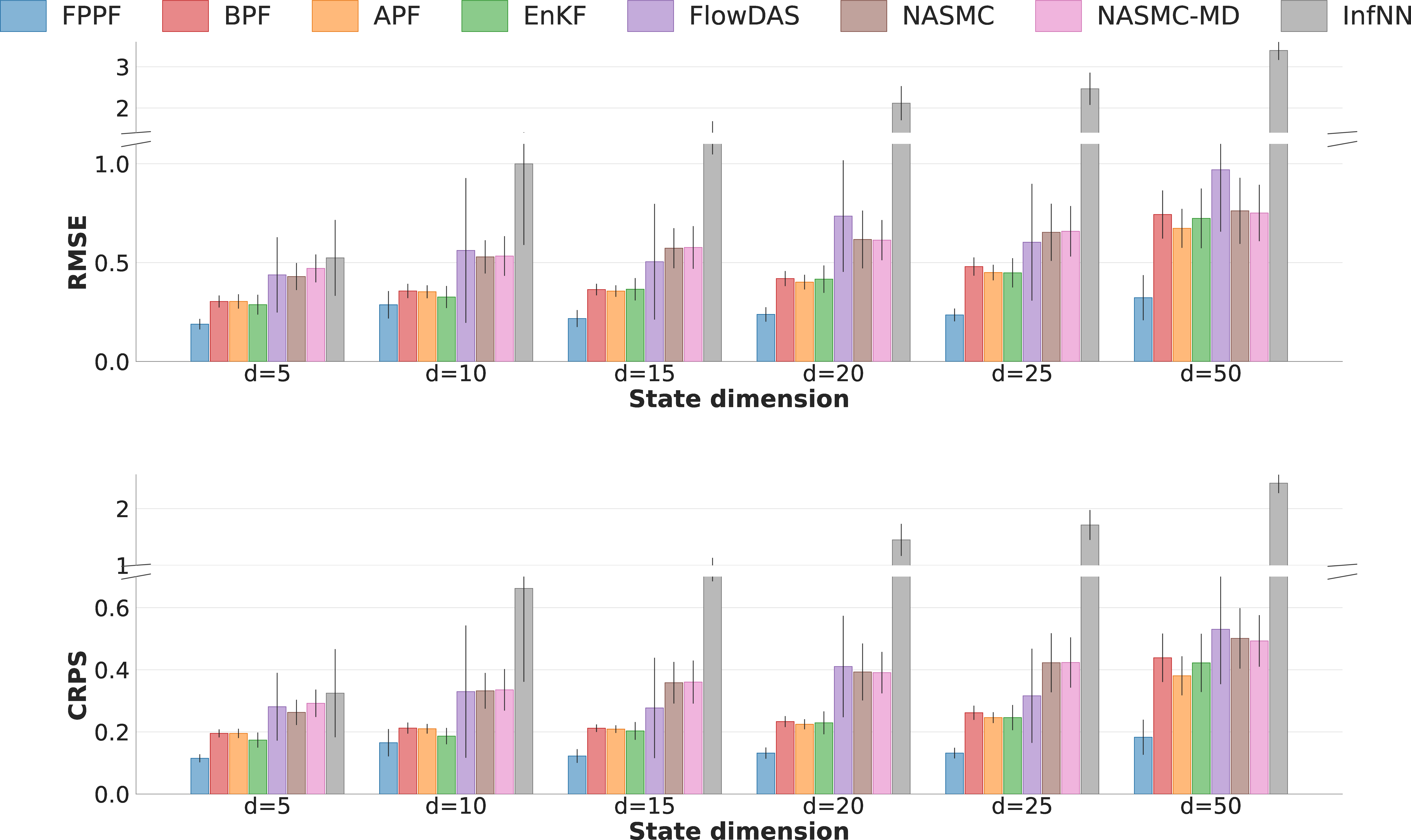
Results. Figure 2 reports results averaged over 100 trajectories of 200 steps, with \(N = 1000\) particles for \(d_x \in \{5, 10\}\) and \(N = 5000\) for \(d_x \in \{15, 20, 25, 50\}\); refer to Appendix 10 for the corresponding table. FPPF achieves the best RMSE and CRPS at every state dimension, and the margin over BPF widens with \(d_x\). Its learned proposal directly targets high-posterior regions by conditioning on observations, whereas the bootstrap proposal uses no observation information and increasingly suffers from the curse of dimensionality. APF, which incorporates observations through auxiliary resampling weights rather than the proposal itself, performs worse than FPPF, but shows gains over BPF that grow with dimension. NASMC also learns an observation-informed proposal but restricts it to a single Gaussian (NASMC-Gauss) or mixture density (NASMC-MD), and underperforms BPF, as does InfNN. EnKF performs slightly better than BPF: under the near-Gaussian likelihood induced by arctan, the Gaussian update used in EnKF remains adequate.
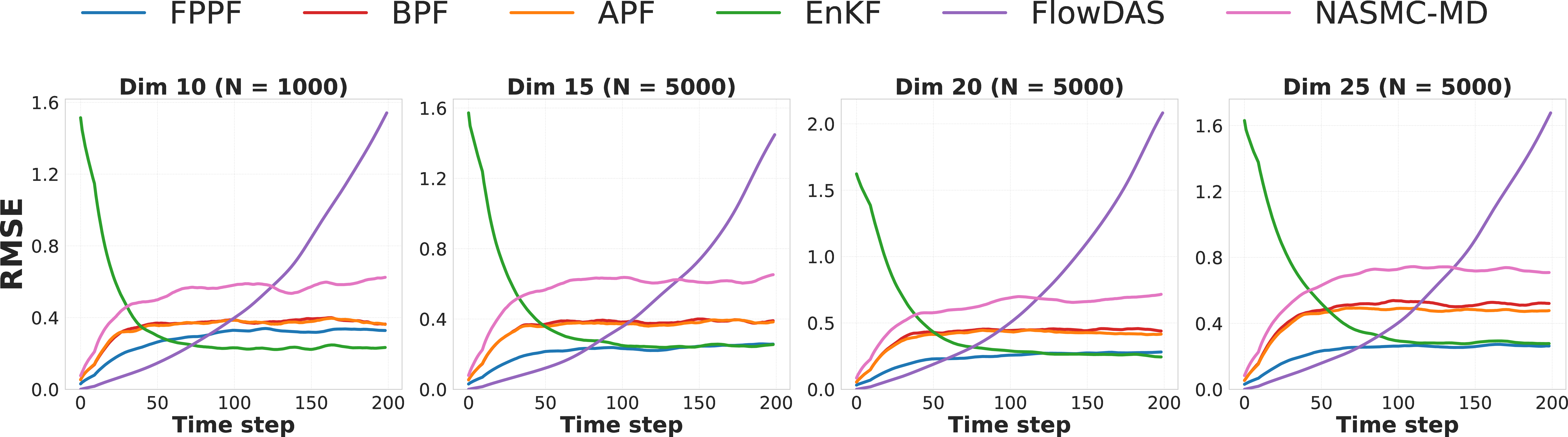
Figure 3 plots RMSE over time for a subset of the baselines. Filtering methods exhibit stable tracking throughout, with FPPF maintaining the lowest error. FlowDAS [25] accumulates error rapidly due to its “single particle” autoregressive generation and lack of principled update step. EnKF has high error early due to poor initialization of sample covariance from the ensemble members.
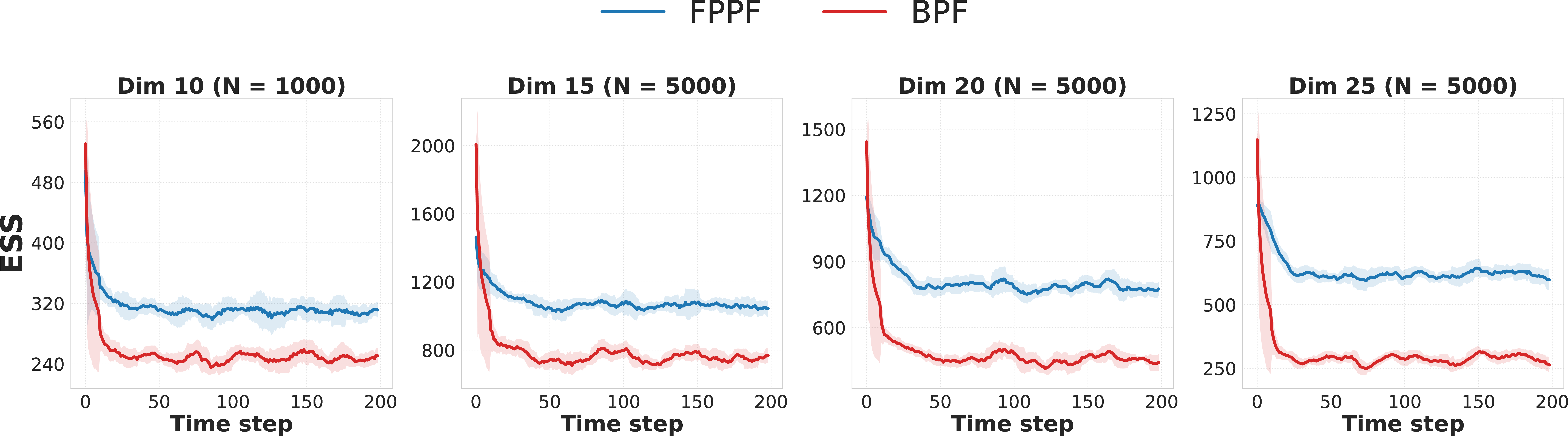
Figure 4 plots pre-resample ESS over time. FPPF maintains a higher ESS than BPF, and the gap widens with dimension. At \(d_x = 25\) the absolute ESS is nonetheless low enough to be concerning, and naively increasing the particle count is computationally infeasible. This motivates the localized variant L-FPPF (Section 5, Section 6.1.2), which exploits the local correlation structure of spatially extended systems to mitigate degeneracy and scale efficiently with state dimensionality.
6.1.2 Localized filters for high-dimensional systems.↩︎
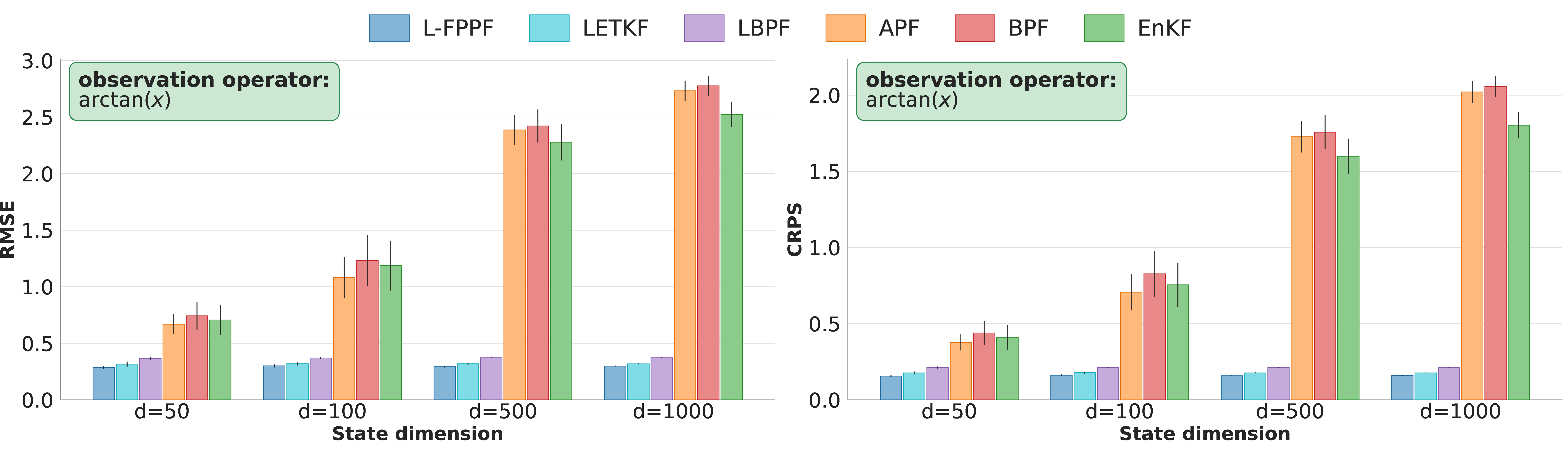
We evaluate L-FPPF on Lorenz-96 at \(d_x = 50\), \(100\), \(500\), and \(1000\), a regime where global particle filters collapse. The L-FPPF proposal is trained once on the \(d_x{=}25\) dataset and applied zero-shot at all four target dimensions. Network inputs have the window dimension \(2r{+}1\), where we fix localization radius \(r{=}4\) across all filtering methods. This allows us to train a lightweight model just once, and the per-step sampling and likelihood integration stays tractable even at \(d_x{=}1000\). Localization also allows us to reduce ensemble size for all PFs to \(N_p{=}500\) particles, with negligible performance decline. While the necessary \(N_p\) for global PFs scale exponentially with the effective state dimension [33], [36], block-wise localization replaces the global problem with overlapping local ones whose effective dimension is set by the localization radius rather than \(d_x\), so the ensemble requirement stays bounded as the state dimension grows [34], [36].
For evaluation, we introduce two localized DA baselines. LETKF [28] performs EnKF analysis in local windows under a Gaussian-posterior assumption and is deployed in operational settings [29], [30]. LBPF [34], [36] propagates particles under global dynamics with tapering local importance weights and per-site resampling; it shares L-FPPF’s block-wise machinery and resampling step, isolating the contribution of the learned local proposal. We also report global BPF, APF, and EnKF for reference.
Results. Figure 5 reports RMSE; the full table including CRPS is in Appendix 11. L-FPPF achieves the lowest RMSE and CRPS at all dimensions, staying relatively flat as \(d_x\) grows from 50 to 1000 while BPF, APF, and EnKF degrade sharply. LBPF is likewise stable with dimension. This is expected, since its block-wise weighting and resampling reduce the effective dimension of the importance-sampling problem from \(d_x\) to a local neighborhood of size set by \(r\). L-FPPF reduces RMSE over LBPF at every dimension. Both filters avoid global particle collapse, but the learned observation-informed proposal places particles nearer the current local posterior, further reducing the residual local weight variance.
6.2 Non-linear and non-Gaussian filtering regimes↩︎
EnKF and related Gaussian-assumption filters are common in operational data assimilation, but their Gaussian posterior approximation breaks down in two key regimes: (i) when the observation operator induces a non-Gaussian observation distribution, and (ii) when the dynamics produce a multimodal prior between observations. We construct experiments that isolate each.
6.2.0.1 Non-Gaussian likelihoods.
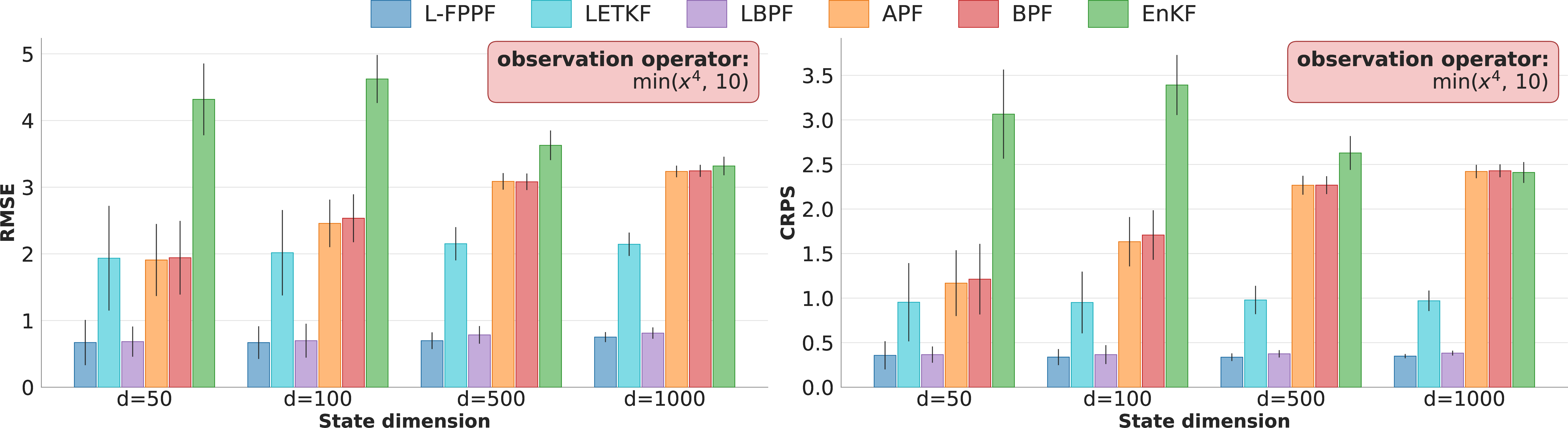
We retain the Lorenz-96 setup of Section 6.1 but replace the arctangent operator with \(h(\mathbf{x}) = \min(\mathbf{x}^4, 10)\) elementwise. This is substantially more challenging: \(\mathbf{x}^4\) is sign-ambiguous, inducing per-component multimodality, and the cap saturates for \(|x_j| > 10^{1/4}\), where the observation carries no magnitude information. Table ¿tbl:tab:lorenz9695quad95capped95s02? reports the same scaling sweep. EnKF fails catastrophically at all dimensions, since a Gaussian posterior cannot represent the induced bimodality. APF also degrades, as its one-step look-ahead is unreliable under a sign-ambiguous, saturating observation model. NASMC-MD recovers some advantage over its Gaussian counterpart by accommodating multimodality. FPPF retains the best RMSE and CRPS at every dimension, with larger margins over BPF than under arctan—likely reflecting the flow proposal’s capacity to learn the multimodal observation-conditional density directly from data. Figure 6 extends the localized comparison to \(d_x \in \{50, 100, 500, 1000\}\) (full table in Appendix 11). LETKF inherits EnKF’s failure mode locally and degrades sharply; LBPF is competitive but still trails L-FPPF.
6.2.0.2 Multimodal distributions.
Lorenz-63 [88] is a three-dimensional chaotic model of atmospheric convection whose attractor has two lobes between which trajectories switch at irregular intervals. The bimodal regime this experiment targets emerges under temporally sparse observations. Between updates the ensemble evolves freely under the nonlinear dynamics, and members straddling a lobe transition are carried into different lobes, so the forecast/prior at the next assimilation time is non-Gaussian and bimodal [89]. Were observations sufficiently frequent, each update would pin the ensemble to the truth within a single lobe and the prior would stay unimodal, leaving little for a non-Gaussian filter to exploit. We therefore assimilate only every 50 integration steps, allowing substantial ensemble dispersion between updates. The state \(\mathbf{x}_t = (x, y, z) \in \mathbb{R}^3\) evolves as \[\dot{x} = \sigma(y - x), \qquad \dot{y} = x(\rho - z) - y, \qquad \dot{z} = xy - \beta z,\] with \(\sigma = 10\), \(\rho = 28\), \(\beta = 8/3\), integrated at \(\Delta t = 0.01\) with process noise \(\sigma_{\mathrm{proc}} = 0.25\). Observations are \(\mathbf{o}_t = \arctan(\mathbf{x}_t) + \mathbf{v}_t\) with \(\mathbf{v}_t \sim \mathcal{N}(\mathbf{0}, \sigma_{\mathrm{obs}}^2 \mathbf{I})\) and \(\sigma_{\mathrm{obs}} = 0.25\).
Table ¿tbl:tab:l6395freq5095results? reports results over 50 trajectories of 1000 steps with \(N = 1000\) particles. FlowDAS is the worst by a wide margin, consistent with the autoregressive error accumulation for long trajectories in previous experiments. Among the remaining filters EnKF is the weakest, its Gaussian posterior is unable to capture the bimodal filtering density, which is precisely the failure this setup isolates. BPF, APF, and FPPF are essentially tied. The bootstrap proposal is adequate here only because the three-dimensional state keeps particle weight variance small, so weights do not collapse (Section 3.2.0.2); this is the low-dimensional regime in which particle filters have always been reliable, and the benefit of an observation-informed proposal instead grows with state dimension (Section 6.1).
\begin{table}[t] 6pt| Metric | BPF | APF | EnKF | FPPF | FlowDAS |
|---|---|---|---|---|---|
| RMSE \(\downarrow\) | 2.7473 \(\pm\) 0.4553 | 2.7650 \(\pm\) 0.4490 | 4.7246 \(\pm\) 0.6827 | 2.7504 \(\pm\) 0.4436 | 7.2579 \(\pm\) 0.9512 |
| CRPS \(\downarrow\) | 1.6760 \(\pm\) 0.2662 | 1.6839 \(\pm\) 0.2617 | 3.0084 \(\pm\) 0.4655 | 1.6755 \(\pm\) 0.2527 | 4.9863 \(\pm\) 0.7024 |
-0.1in \end{table}
6.3 Long-horizon stability under temporally sparse observations↩︎
Operational DA systems must remain stable over long trajectories with observations that are sparse in time. Between observations, the system evolves substantially, the prior at the next observation step can become highly non-Gaussian, and small errors compound across the rollout. We use the Kuramoto-Sivashinsky (KS) equation, a fourth-order nonlinear PDE exhibiting spatiotemporal chaos, to test this regime: \[\partial_t u = -u\, \partial_x u - \partial_x^2 u - \partial_x^4 u,\] with periodic boundary conditions on \([0, L]\), \(L \in \{16\pi, 32\pi\}\). We discretize using a pseudo-spectral method with \(J = 128\) grid points (so \(d_x = J\)), time step \(\Delta t = 0.25\), and process noise \(\sigma_{\mathrm{proc}} = 0.1\). Linearizing about the trivial state \(u \equiv 0\), each Fourier mode grows at rate \(\lambda_k = k^2 - k^4\), so wavenumbers \(0 < |k| < 1\) are linearly unstable. The admissible wavenumbers are \(k = 2\pi n / L\), so a larger domain places more of them in the unstable band; \(L = 16\pi\) admits \(7\) unstable modes and \(L = 32\pi\) admits \(15\). \(L = 32\pi\) is thus the more chaotic, complex regime. All grid points are observed through \[\mathbf{o}_t = h(\mathbf{x}_t) + \mathbf{v}_t, \qquad \mathbf{v}_t \sim \mathcal{N}(\mathbf{0}, \sigma_{\mathrm{obs}}^2 \mathbf{I}), \quad \sigma_{\mathrm{obs}} = 0.1,\] where \(h\) is applied elementwise and is either the smooth \(\arctan\) operator or the sign-ambiguous, saturating \(\min(x^4, 10)\) operator, and observations arrive every 10 steps.
Table 1 reports results over 25 trajectories of 1000 steps using \(N = 5000\) particles, for both observation operators. FlowDAS fails to track the system over the full trajectory in all settings. Under the smooth \(\arctan\) operator, EnKF achieves the lowest error on both domains, with FPPF close behind, since the Gaussian observation update is not heavily violated. Under the more difucult \(\min(x^4, 10)\) operator, FPPF is best on both \(L = 16\pi\) and \(L = 32\pi\). On the more chaotic \(L = 32\pi\) domain FPPF improves the most substantially over BPF. Another proposal learning method, NASMC, also performs well. EnKF performs the worst since its Gaussian likelihood assumption now breaks down under the multimodal observation distribution.
| \(L = 16\pi\) | \(L = 32\pi\) | |||||||
|---|---|---|---|---|---|---|---|---|
| 2-5(l)6-9 | \(\arctan\) | \(\min(z^4,10)\) | \(\arctan\) | \(\min(z^4,10)\) | ||||
| 2-3(lr)4-5(lr)6-7(l)8-9 Method | RMSE \(\downarrow\) | CRPS \(\downarrow\) | RMSE \(\downarrow\) | CRPS \(\downarrow\) | RMSE \(\downarrow\) | CRPS \(\downarrow\) | RMSE \(\downarrow\) | CRPS \(\downarrow\) |
| BPF | 0.14 | 0.08 | 0.91 | 0.65 | 1.21 | 0.84 | 1.59 | 1.17 |
| APF | 0.11 | 0.06 | 0.49 | 0.33 | 0.76 | 0.48 | 1.53 | 1.12 |
| EnKF | 0.07 | 0.05 | 0.18 | 0.12 | 0.11 | 0.06 | 1.65 | 1.17 |
| NASMC-Gauss | 0.09 | 0.05 | 0.15 | 0.08 | 0.19 | 0.10 | 1.24 | 0.82 |
| NASMC-MD | 0.09 | 0.05 | 0.15 | 0.09 | 0.19 | 0.10 | 1.24 | 0.82 |
| InfNN | 1.48 | 1.08 | 1.84 | 1.44 | 1.52 | 1.12 | 1.77 | 1.36 |
| FPPF | 0.09 | 0.05 | 0.11 | 0.06 | 0.19 | 0.10 | 1.15 | 0.76 |
| FlowDAS | 1.18 | 0.70 | 1.55 | 1.12 | 1.23 | 0.72 | 1.62 | 1.18 |
3pt
6.4 Additional experiments↩︎
6.4.0.1 Convergence for linear-Gaussian setting.
To verify that the rectified flow proposal converges to the correct target, we test on a synthetic linear Gaussian state-space model (full settings in Appendix 9), where the locally optimal one-step proposal \(q^\star(\mathbf{x}_t \mid \mathbf{x}_{t-1}, \mathbf{o}_t)\) admits a closed form. Using the same architecture as our L96 experiments, we train \(q_\phi\) on a \(d_x{=}8\) system for 200 epochs.
The left panel of Figure 7 reports the Wasserstein \(W_2\) distance between \(q_\phi\) and \(q^\star\), averaged over \(500\) test set conditioning pairs \((\mathbf{x}_{t-1}, \mathbf{o}_t)\). It decreases over training to 0, indicating convergence to the closed-form optimal proposal. The dotted horizontal line indicates the \(W_2\) distance between the bootstrap proposal \(p(\mathbf{x}_t \mid \mathbf{x}_{t-1})\) and the closed-form optimal proposal \(q^\star(\mathbf{x}_t \mid \mathbf{x}_{t-1}, \mathbf{o}_t)\).
The middle panel reports a one-step ESS. For each conditioning pair we draw \(N{=}250\) samples \(\mathbf{x}_t^{(i)} \sim q_\phi(\cdot \mid \mathbf{x}_{t-1}, \mathbf{o}_t)\), form the one-step SIR importance weights \[\tilde{w}^{(i)} \propto \frac{p(\mathbf{o}_t \mid \mathbf{x}_t^{(i)})\,p(\mathbf{x}_t^{(i)} \mid \mathbf{x}_{t-1})}{q_\phi(\mathbf{x}_t^{(i)} \mid \mathbf{x}_{t-1}, \mathbf{o}_t)},\] and compute \(\mathrm{ESS} = 1 / \sum_i (\bar w^{(i)})^2\) from the normalized weights \(\bar w^{(i)}\), averaging over the \(500\) pairs. This is the ESS the filter would achieve after a single observation update with the proposal. It attains its ceiling of \(N{=}250\) when the incremental weights are uniform (\(\bar w^{(i)} = 1/N\)), which is exactly what the optimal proposal achieves, since under \(q^\star\) the incremental weight is independent of the sampled \(\mathbf{x}_t\) (Eq. 5 ). The bootstrap baseline collapses to near \(80\) (dashed line), while \(q_\phi\) stabilizes near \(250\) over training.
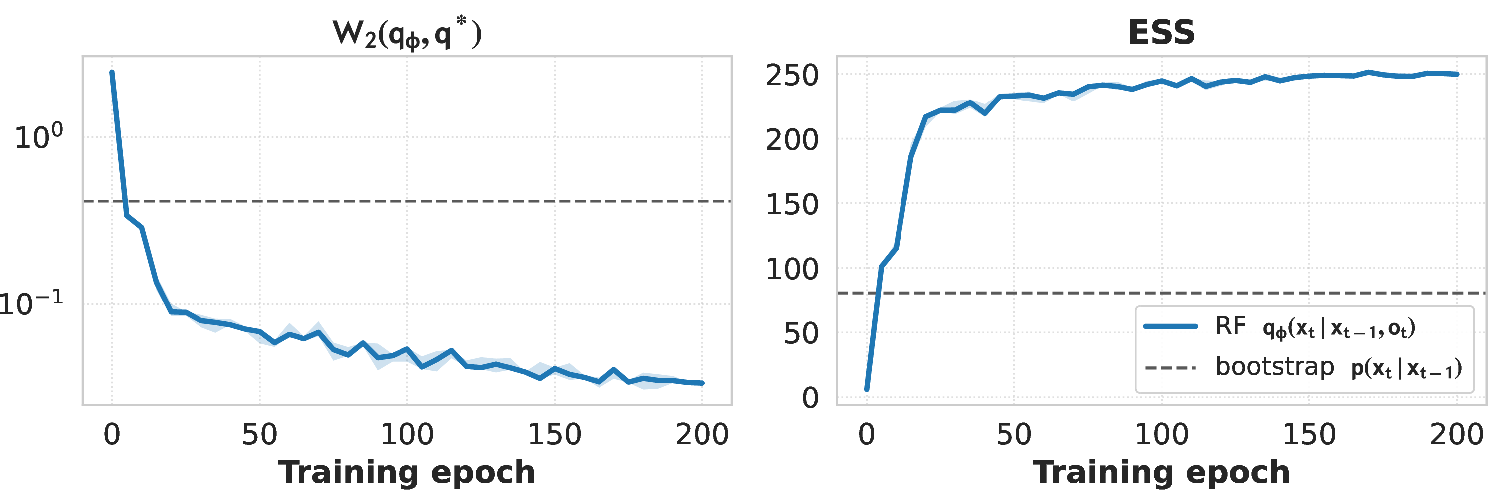
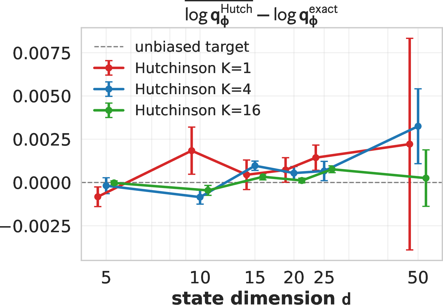
Figure 7: Left: Wasserstein \(W_2\) distance from the learned proposal \(q_\phi\) to the closed-form optimal proposal \(q^\star\) over training epochs, averaged over \(500\) test conditioning pairs; it decreases toward \(0\), while the dashed line is the bootstrap proposal’s \(W_2\) to \(q^\star\). Middle: one-step ESS out of \(N{=}250\) over training epochs; \(q_\phi\) rises toward the maximum of \(250\), while the bootstrap proposal’s (dashed) is near \(80\). Right: bias of the Hutchinson trace estimator relative to the exact trace on the Lorenz-96 proposals across state dimension \(d_x\), for \(K \in \{1, 4, 16\}\) probes; points show mean bias where ideal is 0. Error bars indicate standard deviation across \(N_{\mathrm{pairs}}{=}10\) conditioning pairs..
6.4.0.2 Hutchinson trace estimator.
Computing \(\log q_\phi(\mathbf{x}_t \mid \mathbf{x}_{t-1}, \mathbf{o}_t)\) requires the divergence of the proposal velocity field, which we estimate with the Hutchinson trace estimator (Section 4.2, Eq. 8 ). One concern is that the single-probe estimator (\(K{=}1\)) injects noise into \(\log q_\phi\) and could inflate importance weight variance. We quantify the single-probe estimator error on the trained Lorenz-96 RF proposals from Section 6.1. At \(N_{\mathrm{pairs}}{=}10\) test-set conditioning pairs we draw \(\mathbf{x}_t \sim q_\phi\), evaluate the Hutchinson estimate of \(\log q_\phi\) at \(K \in \{1, 4, 16\}\) probes (\(M{=}200\) random-probe seeds each), and measure its bias and standard deviation against the deterministic exact-trace value. The empirical bias is consistent with zero at every \(d_x\) within pair-to-pair, see Figure 7 (right). Estimator standard deviation stays below \(0.05\) for \(d_x \leq 25\) but grows to \(0.247\) at \(d_x{=}50\) for \(K{=}1\); it is substantially reduced for \(K=16\). While we keep \(K{=}1\) by default for efficiency, at high dimensions increasing \(K\) at the expense of compute may improve performance.
7 Conclusion and Future Work↩︎
We introduced Flow Proposal Particle Filters (FPPF), which replace the bootstrap dynamics with a learned conditional flow proposal approximating the variance-minimizing optimal proposal \(p(\mathbf{x}_t \mid \mathbf{x}_{t-1}, \mathbf{o}_t)\). Conditional flow matching provides efficient sampling and tractable density evaluation, so the SIR weight update remains correct rather than absorbed into approximate guidance. The localized variant L-FPPF uses a patch-based velocity network, making the SIR correction itself decomposable. Across chaotic systems with non-Gaussian likelihoods and long horizons, FPPF and L-FPPF improve state estimation and calibration over classical, learned-proposal, and autoregressive generative baselines, and L-FPPF generalizes to high dimensions zero-shot at fixed ensemble size.
Several directions remain open. A consequential challenge is scaling to operational systems such as ERA5-scale reanalysis [4]. Localization is encouraging in this regard, as it caps the effective dimension at the localization radius rather than the ambient state dimension, allowing methods like L-FPPF to operate stably at large scale with fixed ensemble size. Further, in practice, atmospheric observations are spatially sparse, irregularly distributed, and collected from heterogeneous instruments, with complex, nonlinear observation operators mapping between state and measurement spaces. These features introduce additional structure absent from our benchmarks and can significantly complicate inference. Second, since FPPF assumes access to the transition density for the SIR weight, extending it to data-driven dynamics through a learned forecast emulator is a natural next step. A third concerns cost, as sampling and likelihood evaluation each require multiple integration steps per particle per step; few-step distillation [90]–[92] together with fast divergence estimation [93] could reduce this (Appendix 8.3). Finally, FPPF targets the proposal rather than the analysis distribution, and combining it with latent or score-based ensemble representations is a promising direction we leave to future work.
8 Experimental Setup↩︎
8.1 Data split↩︎
For each system we generate 2048 simulated trajectories and split 80/10/10 into train/validation/test. A subset of the test split is used to report results due to compute constraints; exact subset sizes are listed per experiment.
8.2 FPPF architecture and hyperparameters↩︎
8.2.0.1 Backbone.
For architectural parity, the same backbone with matched parameter count is used as the velocity field in FPPF, the drift network in FlowDAS, and the conditional network in NASMC and InfNN, with only the output head differing across methods. Across all methods we use one of two velocity / feature backbones, picked by spatial structure of the system. (i) For the periodic systems (L96 and KS) the backbone is a 1D ResNet with circular padding and adaptive layer normalization (AdaLN) for flow-time conditioning. Each residual block applies \(\mathrm{AdaLN}(\cdot,s)\!\to\!\mathrm{SiLU}\!\to\! \mathrm{Conv1d}_\mathrm{circ}\!\to\!\mathrm{AdaLN}(\cdot,s)\!\to\! \mathrm{SiLU}\!\to\!\mathrm{Conv1d}_\mathrm{circ}\) with kernel size 5 and a residual skip; AdaLN regresses per-channel \((\gamma, \beta)\) from the flow-time embedding (zero-initialized so the block is initially the identity). The output projection (\(1{\times}1\) conv to one channel) is also zero-initialized. (ii) For the low-dimensional system (L63) the backbone is a flat MLP with SiLU activations and concatenation conditioning. The same body is used as the velocity field in FPPF, the drift in FlowDAS, and the conditional density backbone in NASMC and InfNN; the methods differ only in the output head (vector velocity vs. mixture-of-Gaussians vs.RNADE).
8.2.0.2 Conditioning.
We apply two training-only conditioning regularizers. (1) Similar to classifier-free conditioning dropout with probability \(p_\text{cond}=0.1\) the conditioning \(\mathbf{o}_t\) is zeroed before being fed to the backbone, so the network sees both conditional and unconditional batches with respect to the observation. (2) Previous-state corruption schedule: during training only, with annealed probability \(p(t)=\max(p_\text{min},\, p_0\,(1-t/T))\) we corrupt \(\mathbf{x}_{t-1}\) by zeroing a random subset of its coordinates of size \(\lceil r_\text{mask}\,d_x\rceil\) (no additive Gaussian noise). We use \(p_0=0.3\), \(p_\text{min}=0.05\), \(r_\text{mask}=0.4\), with \(T\) set to the total number of training steps. This forces the conditional network to use \(\mathbf{o}_t\) rather than over-relying on the clean \(\mathbf{x}_{t-1}\) on systems whose forward dynamics is highly predictable. The corruption is disabled at inference.
8.2.0.3 Training
All models are trained for a minimum of 80 epochs, with an early-stopping patience set to 50 epochs.
8.2.0.4 L-FPPF patch network.
The localized velocity field \(u_\phi\) is a small 1D ResNet operating on spatial patches of size \(W = 2r+1\). We use radius \(r = 4\) (so \(W = 9\)), \(C = 64\) channels, 2 residual blocks of kernel size 3, and a 64-dim flow-time embedding fed via AdaLN. Inputs are stacked as a 4-channel window \([\mathbf{z}_{[j-r:j+r]},\,\mathbf{x}_{t-1,[j-r:j+r]},\,\mathbf{o}_{t,[j-r:j+r]}^{\text{full}}, \,m_{t,[j-r:j+r]}]\).
8.3 Baseline Implementation Details↩︎
8.3.0.1 Auxiliary particle filter (APF).
We use the classical Pitt–Shephard [20] auxiliary-particle filter with the prior proposal \(q = p(\mathbf{x}_t \mid \mathbf{x}_{t-1})\) and a point look-ahead. Concretely, the auxiliary adjustment multiplier is \(m_t^{(i)} \;=\; g\!\left(\mathbf{o}_t \,\Big|\, \boldsymbol{\mu}_t^{(i)}\right)\), where \(\boldsymbol{\mu}_t^{(i)} = \mathbb{E}\!\left[\mathbf{x}_t \mid \mathbf{x}_{t-1}^{(i)}\right]\) is the deterministic transition mean (one \(\Delta t\) Euler step of the true dynamics, no process noise). With \(q = p\), the APF incremental weight collapses to \(\log w_t^{(i)} = \log g(\mathbf{o}_t \mid \mathbf{x}_t^{(i)}) - \log m_t^{(k_i)}\), where \(k_i\) is the ancestor selected in the first-stage resample drawn from \(\lambda^{(i)} \propto w_{t-1}^{(i)} m_t^{(i)}\). Weights are reset to the second-stage incremental weight after each step, and a final \(\mathrm{\small ess}<0.33\,N\)-triggered systematic resample is applied to keep the cloud healthy.
8.3.0.2 Ensemble Kalman filter (EnKF).
We use EnKF with multiplicative covariance inflation. The inflation factor is tuned over \(\lambda \in \{0.8, 0.9, 1.0, 1.1\}\) on the validation set and reported at the best-performing \(\lambda\) (lowest RMSE), ensemble size \(N=50\).
8.3.0.3 LETKF.
Our LETKF [28] uses a per-coordinate local analysis on a 1-D periodic spatial domain. For each state index \(j\), observations are tapered by a Gaspari–Cohn polynomial \(\rho(d / r)\) with periodic distance \(d\) (modulo \(d_x\)) and localization radius \(r\), the local symmetric square-root analysis is solved in ensemble space, and the resulting analysis ensemble member \(\mathbf{x}^{(i)}_j\) is assembled by stacking centre-coordinate analyses We tune inflation factor on a held-out validation subset over \(\lambda \in \{0.8,0.9,\ldots,1.8\}\) and set \(r\) to match other localized baselines. For the L96-25 in-distribution and high-dim (\(d_x \in \{50, 100, 500, 1000\}\)) cells we use \(r=4\) (matched to the L-FPPF localization radius of \(r=4\) patches), \(\lambda=1.0\), ensemble size \(N=50\).
8.3.0.4 LBPF.
The localized BPF is the block-localized particle filter of [36]: the spatial domain is partitioned into contiguous blocks and the analysis weights, ancestor resampling, and patchwork particle reassembly are computed independently within each block on tapered local likelihoods. We use block size 1 (per-coordinate analysis), with localization radius \(r=4\) (matched to L-FPPF), and systematic local resampling with the identity-preserving (adjustment-minimizing) ancestor-permutation tie-break of [36]. No post-regularization jitter is applied.
8.3.0.5 FlowDAS.
For all FlowDAS experiments [25] we use the official implementation. The guidance scale is set to 0.01 (selected via ablation), \(J=21\) Monte Carlo sampling times, learning rate \(3\times10^{-4}\) with early stopping. Inference uses 50 first-order Euler steps. FlowDAS does not produce an ensemble by default; for CRPS we draw 20 independent rollouts per evaluation trajectory and compute CRPS from this empirical predictive distribution.
8.3.0.6 NASMC.
We follow [39] and report two variants: NASMC\(_{K{=}1}\), the single-Gaussian baseline of [39], and NASMC\(_{K{=}3}\), the “-MD-” mixture-density variant with \(K=3\)
components (paper default). We do not use the paper’s LSTM history conditioning; conditioning is Markovian on \((\mathbf{x}_{t-1},
\mathbf{o}_t)\), matching the FPPF / InfNN comparison. At evaluation, the trained \(q_\phi\) is plugged into our standard BPF and inherits all per-cell PF settings (\(N\), ESS
threshold, \(\sigma_x\), \(\sigma_y\), batch size) from the corresponding FPPF cell.
8.3.0.7 InfNN.
We use InfNN-RNADE variant from the paper: coordinates are factorized in their natural index order \(\prod_{j=1}^{d_x} q_\phi(x_t^{(j)} \mid x_t^{(<j)}, \mathbf{x}_{t-1},
\mathbf{o}_t)\), with each factor a \(K=3\)-component diagonal Gaussian mixture produced by a \(2\)-layer MLP of hidden size \(128\) (rnade head, mirroring the original paper). At evaluation, the trained \(q_\phi\) is plugged into our standard BPF and inherits all per-cell PF settings (\(N\), ESS
threshold, \(\sigma_x\), \(\sigma_y\), batch size) from the corresponding FPPF cell.
8.4 Inference time proposal cost↩︎
For all experiments we use \(N_s = N_\ell = 32\) Euler integration steps for both forward sampling and reverse likelihood evaluation, on a uniform time grid for sampling and a \(\gamma{=}2\) non-uniform power-back grid for likelihood, where \(s_k = 1 - (1-u_k)^{\gamma}\), \(\gamma > 1\). This results in smaller step sizes closer to the target distribution. Empirically, we find that the non-uniform grid allowed us to decrease the number of integration steps from 100 to 32 with minimal performance degradation, compared to a uniform grid. A natural direction to reduce the inference-time cost of FPPF, which currently runs \(\sim\)32-step Euler integration twice per particle per step (once for sampling, once for likelihood evaluation), is to replace the rectified-flow teacher with a few-step student. Recent work on consistency models [90], MeanFlow [91], and Shortcut models [92] produces high-quality samples in one or a handful of NFEs, and the F2D2 framework [93] extends this idea to fast divergence estimation, opening a path to also accelerate the likelihood evaluation step rather than only sampling. In our preliminary experiments, however, we found that the resulting few-step proposals were of substantially lower quality than the teacher: students tended to collapse toward the conditional mean, eroding the observation-informed structure that makes the proposal useful in the first place, and the residual bias in the distilled divergence degraded ESS over long horizons. We therefore report the 32-step teacher throughout the main paper. Bridging the gap between distillation quality and proposal informativeness is an interesting direction for reducing the compute cost of FPPF.
9 Linear-Gaussian System Details↩︎
9.0.0.1 System.
We use \(d_x{=}8\) with \(\mathbf{x}_t = \mathbf{A} \mathbf{x}_{t-1} + \mathbf{w}_t\), \(\mathbf{o}_t = \mathbf{H} \mathbf{x}_t + \mathbf{v}_t\), where \(\mathbf{w}_t \sim \mathcal{N}(\mathbf{0}, \mathbf{Q})\), \(\mathbf{v}_t \sim \mathcal{N}(\mathbf{0}, \mathbf{R})\), and \(\mathbf{x}_0 \sim \mathcal{N}(\mathbf{0}, \mathbf{I})\). Writing \(\mathbf{S}\) for the cyclic shift and \(\mathbf{C}(\alpha)_{ij} = \alpha^{|i-j|}\) for a Toeplitz correlation, we set \(\mathbf{A} = 0.92\,\mathbf{I} + 0.05\,\mathbf{S} + 0.02\,\mathbf{S}^{\!\top}\), \(\mathbf{H} = \mathbf{I} + 0.25\,\mathbf{S} - 0.15\,\mathbf{S}^{\!\top}\), \(\mathbf{Q} = 0.35^2(0.7\,\mathbf{I} + 0.3\,\mathbf{C}(0.5))\), \(\mathbf{R} = 0.25^2(0.6\,\mathbf{I} + 0.4\,\mathbf{C}(0.7))\). \(\mathbf{A}\) is stable (\(\rho(\mathbf{A}){<}1\)), \(\mathbf{H}\) mixes neighbours asymmetrically, and both noises are spatially correlated. All states are observed.
9.0.0.2 Dataset.
\(N_\text{traj}{=}1024\) trajectories of length \(T{=}200\) after a \(100\)-step burn-in, split \(80/10/10\) by trajectory into train / val / test.
9.0.0.3 Optimal proposal.
For this system \(q^\star(\mathbf{x}_t \mid \mathbf{x}_{t-1}, \mathbf{o}_t)\) is Gaussian with \[\mathbf{K} = \mathbf{Q} \mathbf{H}^{\!\top}(\mathbf{H} \mathbf{Q} \mathbf{H}^{\!\top} + \mathbf{R})^{-1}, \quad \boldsymbol{\mu}^\star = \mathbf{A} \mathbf{x}_{t-1} + \mathbf{K}(\mathbf{o}_t - \mathbf{H} \mathbf{A} \mathbf{x}_{t-1}), \quad \boldsymbol{\Sigma}^\star = (\mathbf{I} - \mathbf{K} \mathbf{H})\mathbf{Q}.\] \(\boldsymbol{\Sigma}^\star\) is independent of \((\mathbf{x}_{t-1}, \mathbf{o}_t)\), so all conditioning enters through \(\boldsymbol{\mu}^\star\). This is the target the learned proposal \(q_\phi\) must match.
9.0.0.4 Bootstrap reference.
The dynamics prior \(q_b(\mathbf{x}_t \mid \mathbf{x}_{t-1}) = \mathcal{N}(\mathbf{A} \mathbf{x}_{t-1}, \mathbf{Q})\) ignores \(\mathbf{o}_t\) and serves as the floor a useful learned proposal must beat.
10 Full Lorenz-96 Results↩︎
Complete results are in Table ¿tbl:tab:lorenz9695arctan95s02? and Table ¿tbl:tab:lorenz9695quad95capped95s02?.
\begin{table}[!t]| State Dimension \(d_x\) | ||||||
|---|---|---|---|---|---|---|
| 2-7 Method | 5 | 10 | 15 | 20 | 25 | 50 |
| RMSE \(\downarrow\) | ||||||
| BPF | 0.303 \(\pm\) 0.030 | 0.357 \(\pm\) 0.036 | 0.364 \(\pm\) 0.029 | 0.419 \(\pm\) 0.038 | 0.480 \(\pm\) 0.046 | 0.743 \(\pm\) 0.122 |
| APF | 0.304 \(\pm\) 0.036 | 0.353 \(\pm\) 0.033 | 0.356 \(\pm\) 0.029 | 0.401 \(\pm\) 0.037 | 0.450 \(\pm\) 0.039 | 0.673 \(\pm\) 0.099 |
| EnKF | 0.287 \(\pm\) 0.050 | 0.326 \(\pm\) 0.056 | 0.365 \(\pm\) 0.056 | 0.416 \(\pm\) 0.069 | 0.448 \(\pm\) 0.074 | 0.724 \(\pm\) 0.151 |
| NASMC-Gauss | 0.430 \(\pm\) 0.068 | 0.529 \(\pm\) 0.084 | 0.573 \(\pm\) 0.101 | 0.617 \(\pm\) 0.146 | 0.653 \(\pm\) 0.145 | 0.762 \(\pm\) 0.167 |
| NASMC-MD | 0.471 \(\pm\) 0.071 | 0.533 \(\pm\) 0.100 | 0.577 \(\pm\) 0.108 | 0.614 \(\pm\) 0.102 | 0.659 \(\pm\) 0.128 | 0.751 \(\pm\) 0.143 |
| InfNN | 0.524 \(\pm\) 0.192 | 1.000 \(\pm\) 0.411 | 1.363 \(\pm\) 0.316 | 2.117 \(\pm\) 0.415 | 2.467 \(\pm\) 0.392 | 3.396 \(\pm\) 0.231 |
| FPPF | 0.189 \(\pm\) 0.027 | 0.287 \(\pm\) 0.070 | 0.217 \(\pm\) 0.043 | 0.238 \(\pm\) 0.037 | 0.235 \(\pm\) 0.032 | 0.323 \(\pm\) 0.114 |
| FlowDAS | 0.438 \(\pm\) 0.191 | 0.562 \(\pm\) 0.366 | 0.505 \(\pm\) 0.293 | 0.735 \(\pm\) 0.282 | 0.603 \(\pm\) 0.295 | 0.970 \(\pm\) 0.313 |
| CRPS \(\downarrow\) | ||||||
| BPF | 0.195 \(\pm\) 0.013 | 0.212 \(\pm\) 0.018 | 0.212 \(\pm\) 0.012 | 0.233 \(\pm\) 0.018 | 0.262 \(\pm\) 0.023 | 0.439 \(\pm\) 0.078 |
| APF | 0.195 \(\pm\) 0.015 | 0.210 \(\pm\) 0.016 | 0.209 \(\pm\) 0.012 | 0.225 \(\pm\) 0.016 | 0.246 \(\pm\) 0.018 | 0.381 \(\pm\) 0.063 |
| EnKF | 0.174 \(\pm\) 0.024 | 0.186 \(\pm\) 0.026 | 0.203 \(\pm\) 0.029 | 0.229 \(\pm\) 0.037 | 0.246 \(\pm\) 0.041 | 0.422 \(\pm\) 0.094 |
| NASMC-Gauss | 0.263 \(\pm\) 0.041 | 0.332 \(\pm\) 0.058 | 0.358 \(\pm\) 0.067 | 0.393 \(\pm\) 0.092 | 0.423 \(\pm\) 0.095 | 0.501 \(\pm\) 0.097 |
| NASMC-MD | 0.292 \(\pm\) 0.044 | 0.336 \(\pm\) 0.067 | 0.360 \(\pm\) 0.069 | 0.391 \(\pm\) 0.067 | 0.423 \(\pm\) 0.081 | 0.493 \(\pm\) 0.083 |
| InfNN | 0.325 \(\pm\) 0.142 | 0.662 \(\pm\) 0.301 | 0.908 \(\pm\) 0.224 | 1.448 \(\pm\) 0.283 | 1.711 \(\pm\) 0.264 | 2.450 \(\pm\) 0.176 |
| FPPF | 0.115 \(\pm\) 0.013 | 0.165 \(\pm\) 0.044 | 0.122 \(\pm\) 0.022 | 0.132 \(\pm\) 0.018 | 0.132 \(\pm\) 0.017 | 0.183 \(\pm\) 0.056 |
| FlowDAS | 0.281 \(\pm\) 0.109 | 0.330 \(\pm\) 0.213 | 0.277 \(\pm\) 0.162 | 0.411 \(\pm\) 0.163 | 0.316 \(\pm\) 0.152 | 0.530 \(\pm\) 0.177 |
-0.1in \end{table}
\begin{table}[!t]| State Dimension \(d_x\) | ||||||
|---|---|---|---|---|---|---|
| 2-7 Method | 5 | 10 | 15 | 20 | 25 | 50 |
| RMSE \(\downarrow\) | ||||||
| BPF | 0.279 \(\pm\) 0.034 | 0.411 \(\pm\) 0.070 | 0.404 \(\pm\) 0.051 | 0.591 \(\pm\) 0.318 | 0.803 \(\pm\) 0.474 | 1.942 \(\pm\) 0.552 |
| APF | 0.288 \(\pm\) 0.032 | 0.416 \(\pm\) 0.061 | 0.429 \(\pm\) 0.071 | 0.606 \(\pm\) 0.367 | 0.772 \(\pm\) 0.471 | 1.878 \(\pm\) 0.560 |
| EnKF | 0.757 \(\pm\) 0.976 | 1.661 \(\pm\) 1.580 | 2.621 \(\pm\) 1.543 | 3.157 \(\pm\) 1.319 | 3.474 \(\pm\) 1.149 | 4.353 \(\pm\) 0.531 |
| NASMC-Gauss | 0.556 \(\pm\) 0.332 | 0.957 \(\pm\) 0.690 | 1.060 \(\pm\) 0.650 | 1.248 \(\pm\) 0.699 | 1.502 \(\pm\) 0.707 | 1.425 \(\pm\) 0.486 |
| NASMC-MD | 0.639 \(\pm\) 0.419 | 0.857 \(\pm\) 0.616 | 1.050 \(\pm\) 0.574 | 1.416 \(\pm\) 0.796 | 1.184 \(\pm\) 0.628 | 1.605 \(\pm\) 0.514 |
| InfNN | 0.962 \(\pm\) 1.086 | 3.282 \(\pm\) 0.914 | 3.599 \(\pm\) 0.624 | 4.213 \(\pm\) 0.425 | 4.314 \(\pm\) 0.424 | 4.726 \(\pm\) 0.262 |
| FPPF | 0.201 \(\pm\) 0.032 | 0.321 \(\pm\) 0.125 | 0.237 \(\pm\) 0.059 | 0.382 \(\pm\) 0.310 | 0.254 \(\pm\) 0.068 | 0.519 \(\pm\) 0.298 |
| FlowDAS | 0.354 \(\pm\) 0.132 | 0.560 \(\pm\) 0.387 | 0.510 \(\pm\) 0.283 | 0.740 \(\pm\) 0.288 | 0.629 \(\pm\) 0.320 | 0.945 \(\pm\) 0.321 |
| CRPS \(\downarrow\) | ||||||
| BPF | 0.205 \(\pm\) 0.013 | 0.250 \(\pm\) 0.036 | 0.242 \(\pm\) 0.023 | 0.332 \(\pm\) 0.176 | 0.456 \(\pm\) 0.307 | 1.213 \(\pm\) 0.396 |
| APF | 0.207 \(\pm\) 0.013 | 0.250 \(\pm\) 0.030 | 0.253 \(\pm\) 0.033 | 0.342 \(\pm\) 0.226 | 0.431 \(\pm\) 0.302 | 1.143 \(\pm\) 0.385 |
| EnKF | 0.520 \(\pm\) 0.772 | 1.145 \(\pm\) 1.203 | 1.761 \(\pm\) 1.157 | 2.102 \(\pm\) 1.022 | 2.368 \(\pm\) 0.941 | 3.102 \(\pm\) 0.491 |
| NASMC-Gauss | 0.358 \(\pm\) 0.263 | 0.657 \(\pm\) 0.539 | 0.703 \(\pm\) 0.456 | 0.823 \(\pm\) 0.482 | 0.961 \(\pm\) 0.487 | 0.901 \(\pm\) 0.311 |
| NASMC-MD | 0.423 \(\pm\) 0.335 | 0.581 \(\pm\) 0.472 | 0.697 \(\pm\) 0.410 | 0.920 \(\pm\) 0.542 | 0.773 \(\pm\) 0.421 | 0.995 \(\pm\) 0.333 |
| InfNN | 0.684 \(\pm\) 0.915 | 2.441 \(\pm\) 0.747 | 2.606 \(\pm\) 0.538 | 3.149 \(\pm\) 0.381 | 3.227 \(\pm\) 0.401 | 3.651 \(\pm\) 0.244 |
| FPPF | 0.125 \(\pm\) 0.017 | 0.191 \(\pm\) 0.083 | 0.134 \(\pm\) 0.032 | 0.223 \(\pm\) 0.205 | 0.142 \(\pm\) 0.037 | 0.289 \(\pm\) 0.143 |
| FlowDAS | 0.233 \(\pm\) 0.075 | 0.331 \(\pm\) 0.229 | 0.283 \(\pm\) 0.154 | 0.411 \(\pm\) 0.163 | 0.330 \(\pm\) 0.165 | 0.511 \(\pm\) 0.181 |
-0.1in \end{table}
11 Full High-dimensional Lorenz-96 Results↩︎
Complete results are in Table ¿tbl:tab:lorenz9695highdim95arctan95s02? and Table ¿tbl:tab:lorenz9695highdim95quartic95capped95s02?.
\begin{table}[!t] 5pt@lcccc@ &
(l)2-5 Method & 50 & 100 & 500 & 1000
L-FPPF & 0.287 \(\pm\) 0.012 & 0.300 \(\pm\) 0.014 & 0.293 \(\pm\) 0.007 & 0.299
\(\pm\) 0.004
LETKF & 0.316 \(\pm\) 0.022 & 0.319 \(\pm\) 0.015 & 0.319 \(\pm\) 0.007 & 0.318 \(\pm\) 0.004
LBPF & 0.366 \(\pm\) 0.016 & 0.370 \(\pm\) 0.011 & 0.372 \(\pm\) 0.005 & 0.372 \(\pm\) 0.004
APF & 0.669 \(\pm\) 0.087 & 1.082 \(\pm\) 0.183 & 2.386 \(\pm\) 0.135 & 2.732 \(\pm\) 0.089
BPF & 0.743 \(\pm\) 0.122 & 1.232 \(\pm\) 0.224 & 2.421 \(\pm\) 0.146 & 2.776 \(\pm\) 0.090
EnKF & 0.706 \(\pm\) 0.133 & 1.187 \(\pm\) 0.220 & 2.278 \(\pm\) 0.162 & 2.522 \(\pm\) 0.109
L-FPPF & 0.156 \(\pm\) 0.006 & 0.162 \(\pm\) 0.006 & 0.158 \(\pm\) 0.003 & 0.161
\(\pm\) 0.002
LETKF & 0.177 \(\pm\) 0.009 & 0.178 \(\pm\) 0.006 & 0.177 \(\pm\) 0.003 & 0.177 \(\pm\) 0.002
LBPF & 0.212 \(\pm\) 0.007 & 0.213 \(\pm\) 0.004 & 0.213 \(\pm\) 0.002 & 0.213 \(\pm\) 0.002
APF & 0.377 \(\pm\) 0.053 & 0.707 \(\pm\) 0.120 & 1.727 \(\pm\) 0.103 & 2.021 \(\pm\) 0.072
BPF & 0.439 \(\pm\) 0.078 & 0.827 \(\pm\) 0.150 & 1.757 \(\pm\) 0.110 & 2.058 \(\pm\) 0.070
EnKF & 0.411 \(\pm\) 0.082 & 0.755 \(\pm\) 0.144 & 1.599 \(\pm\) 0.116 & 1.803 \(\pm\) 0.084
-0.1in \end{table}
\begin{table}[!t] 5pt@lcccc@ &
(l)2-5 Method & 50 & 100 & 500 & 1000
L-FPPF & 0.670 \(\pm\) 0.339 & 0.669 \(\pm\) 0.245 & 0.698 \(\pm\) 0.125 & 0.752
\(\pm\) 0.075
LETKF & 1.935 \(\pm\) 0.785 & 2.017 \(\pm\) 0.640 & 2.152 \(\pm\) 0.249 & 2.144 \(\pm\) 0.175
LBPF & 0.684 \(\pm\) 0.226 & 0.698 \(\pm\) 0.254 & 0.785 \(\pm\) 0.132 & 0.812 \(\pm\) 0.085
APF & 1.908 \(\pm\) 0.540 & 2.457 \(\pm\) 0.356 & 3.087 \(\pm\) 0.124 & 3.236 \(\pm\) 0.087
BPF & 1.942 \(\pm\) 0.552 & 2.534 \(\pm\) 0.359 & 3.081 \(\pm\) 0.124 & 3.245 \(\pm\) 0.090
EnKF & 4.317 \(\pm\) 0.538 & 4.623 \(\pm\) 0.360 & 3.628 \(\pm\) 0.222 & 3.318 \(\pm\) 0.139
L-FPPF & 0.358 \(\pm\) 0.158 & 0.338 \(\pm\) 0.090 & 0.337 \(\pm\) 0.043 & 0.349
\(\pm\) 0.024
LETKF & 0.954 \(\pm\) 0.439 & 0.951 \(\pm\) 0.346 & 0.979 \(\pm\) 0.159 & 0.970 \(\pm\) 0.115
LBPF & 0.366 \(\pm\) 0.091 & 0.366 \(\pm\) 0.106 & 0.375 \(\pm\) 0.041 & 0.383 \(\pm\) 0.027
APF & 1.168 \(\pm\) 0.369 & 1.633 \(\pm\) 0.277 & 2.267 \(\pm\) 0.106 & 2.421 \(\pm\) 0.075
BPF & 1.213 \(\pm\) 0.396 & 1.708 \(\pm\) 0.278 & 2.268 \(\pm\) 0.100 & 2.429 \(\pm\) 0.072
EnKF & 3.065 \(\pm\) 0.500 & 3.392 \(\pm\) 0.337 & 2.629 \(\pm\) 0.190 & 2.410 \(\pm\) 0.117
-0.1in \end{table}
References↩︎
Correspondence to:
cnagda2@illinois.edu↩︎