The Binary Tree Mechanism is Optimal for Approximate Differentially Private Continual Counting
July 01, 2026
Abstract
Private continual counting is a fundamental problem in differential privacy: given a binary stream of length \(n\), where each \(1\) corresponds to the contribution of one individual, the goal is to release all running counts while protecting the privacy of each individual. The standard algorithm is the binary tree mechanism, whose Gaussian-noise variant achieves expected \(\ell_\infty\) error proportional to \(\log^{3/2} n\) for approximate differential privacy. Whether this dependence on the stream length is necessary has remained a central open problem.
In this work, we resolve the dependence on \(n\) by proving that every differentially private mechanism for continual counting must incur expected \(\ell_\infty\) error \(\Omega(\log^{3/2} n)\). This shows that the binary tree mechanism is asymptotically optimal in the approximate-DP setting.
As a consequence, we also obtain a largest-possible separation between hereditary discrepancy and private \(\ell_\infty\) error for linear queries, showing that the known general upper bound in terms of hereditary discrepancy has the optimal dependence on the number of queries.
1 Introduction↩︎
How can an organization track the occurrence of sensitive events over time without compromising the privacy of individuals? Such scenarios arise naturally in many settings, including monitoring daily disease cases, counting user interactions on a platform, or measuring responses to a public poll. This motivates the study of private continual counting, the focus of this paper. The standard formulation of the problem models time as discrete steps \(1, \ldots, n\), where at each step a bit indicates whether an event occurred. Each \(1\) corresponds to the contribution of one individual and each individual participates in at most one event. The goal is to release an accurate running count at every time step without revealing any individual’s contribution.
The study of private continual counting was initiated by [1], [2], who established the foundations for differentially private computations under continual observation. Differential privacy (DP) [3] is the standard framework for formal privacy guarantees, ensuring that the output of a mechanism reveals little about any individual’s data. Private continual counting has found applications in a broad range of tasks including private online learning [4], [5], convex optimization [6] and federated learning [7]. In many of these applications, it appears as a subroutine, and improving its accuracy directly translates to improvements in the downstream task. The appropriate notion of error, however, depends on the application: \(\ell_\infty\) error (the expected worst-case error over all time steps) is a natural measure for monitoring tasks, while \(\ell_2\) error (the expected root mean squared error over all time steps) is more relevant for learning applications [8]. In this work, we focus on the \(\ell_\infty\) error.
The most well-known method for private continual counting is the binary tree mechanism [1], [2], which computes carefully structured subset counts in a differentially private manner and combines them to recover the running count at any given time step.
For pure differential privacy, the binary tree mechanism uses Laplace noise to make the subset counts \(\varepsilon\)-differentially private. Here, and throughout the paper, we focus on the regime where \(\varepsilon\in (0,1)\). While the original analysis achieves \(\ell_\infty\) error \(O(\log^{5/2} (n)/\varepsilon)\) [1], [2], a more careful analysis of the same algorithm yields an improved bound of \(O(\log^2 (n)/\varepsilon)\). The best known lower bound is \(\Omega(\log (n)/\varepsilon)\) [1], leaving a multiplicative gap of \(\log n\).
For approximate DP, the binary tree mechanism uses Gaussian noise instead of Laplace, yielding an \((\varepsilon, \delta)\)-differentially private mechanism with \(\ell_\infty\) error \(O(\log^{3/2} (n) \sqrt{\log(1/\delta)}/\varepsilon)\) [9]. Prior to our work, the best known lower bound related to the \(\ell_\infty\) error under approximate DP was an \(\Omega(\log (n)/\varepsilon)\) lower bound on the square root of the expected value of the square of the worst-case error over all \(n\) time steps (\(\sqrt{\ell_{\infty}^2}\) error) [10].
Whether the \(\ell_\infty\) error upper bounds are tight in the dependency on the stream length \(n\) has remained an important open problem. In this work, we resolve the approximate DP setting by proving a lower bound of \(\Omega(\log^{3/2}(n)/\max\{\varepsilon,\delta\})\). For \(\delta = 0\), this applies to pure DP, tightening the gap there as well. 1 summarizes the best known upper and lower bounds for pure and approximate DP with \(\varepsilon\in (0,1)\).
| Setting | Error Notion | Upper Bound | Lower Bound | |
|---|---|---|---|---|
| Pure DP | \(\ell_\infty\) error | \(\log^{2}(n)/\varepsilon\) | \(\log^{3/2}(n)/\varepsilon\) [Our result] | |
| Approx. DP | \(\ell_\infty\) error | \(\log^{3/2}(n)\log^{1/2}(1/\delta)/\varepsilon\) [9] | \(\log^{3/2}(n)/\max\{\varepsilon,\delta\}\) [Our result] | |
| \(\sqrt{\ell_\infty^2}\) error | \(\log(n)/\varepsilon\) [10] |
Before stating our result, we formally define the problem of private continual counting and the privacy notion we work with. Let \(x \in \{0,1\}^n\) be the binary input vector, where \(x_i = 1\) indicates that an event occurred at time step \(i\) and since the mechanism operates in an online fashion, at time step \(i\) only the entries \(x_1, \ldots, x_i\) are visible to it. The goal is to approximate, at each time step \(i\), the running count \(\sum_{j\leq i}x_j\) in a differentially private manner. These \(n\) running counts can be written compactly as \(Ax\), where \(A\) is the \(n \times n\) lower triangular matrix of all ones, known as the prefix-sum matrix, with \((Ax)_i=\sum_{j \leq i} x_j\). This problem can be seen as a specific instance of linear queries (mechanisms that answer queries of the form \(Ax\) for a fixed matrix \(A\)), where the query matrix is the prefix-sum matrix \(A\). A private mechanism \(\mathbf{M}\) must output a vector \(\mathbf{M}(x) \in \mathbb{R}^n\), where \(\mathbf{M}(x)_i\) is the estimate released at time step \(i\), so that \(\|\mathbf{M}(x)-Ax\|_\infty\) is small while ensuring privacy of any individual’s entry in \(x\). With this notation, the \(\ell_\infty\) error is \(\mathbb{E}[\|\mathbf{M}(x)-Ax\|_\infty]\), whereas the \(\ell_2\) error is \(n^{-1/2}\mathbb{E}[\|\mathbf{M}(x)-Ax\|_2]\).
We say that two binary vectors \(x,x' \in \{0,1\}^n\) are neighboring if they differ in exactly one coordinate. The mechanism \(\mathbf{M}\) is required to satisfy differential privacy, defined as follows.
Definition 1 (Differential Privacy [3]). Fix \(\varepsilon> 0\) and \(\delta \in [0,1)\). A mechanism \(\mathbf{M}\) is \((\varepsilon,\delta)\)-DP if for any measurable set \(S \subseteq \mathbb{R}^n\), \[\Pr[\mathbf{M}(x) \in S] \leq e^\varepsilon\Pr[\mathbf{M}(x') \in S]+\delta\] for all pairs of neighboring inputs \(x,x' \in \{0,1\}^n\).
The case where \(\delta = 0\) is referred to as pure DP and the case where \(\delta > 0\) is referred to as approximate DP.
Our main result establishes a fundamental lower bound on the \(\ell_\infty\) error of any \((\varepsilon, \delta)\)-DP mechanism for continual counting.
Theorem 1. For any \(0 < \varepsilon< 1\), \(0 < \delta < C\) for a sufficiently small constant \(C>0\), it holds that any \((\varepsilon,\delta)\)-DP mechanism \(\mathbf{M}\) for continual counting has error \[\max_{x \in \{0,1\}^n }\mathbb{E}[\|\mathbf{M}(x)-Ax\|_\infty] = \Omega\left(\frac{\log^{3/2} n }{\max\{\varepsilon,\delta\}}\right),\] where \(A\) is the \(n \times n\) prefix-sum matrix.
This shows that the binary tree mechanism has an asymptotically optimal dependency on \(n\) in the approximate DP setting.
We now make a few observations about the lower bound in 1. The binary tree mechanism can operate in both the continual observation model, where the input stream arrives online, and the offline observation model [11], where the mechanism receives the entire input stream at once. Our lower bound holds in the offline observation model and, since any mechanism for continual observation also yields a mechanism for offline observation, lower bounds in the offline model imply lower bounds for the continual observation model. Specifically, such lower bounds emphasize that the hardness comes from releasing \(n\) outputs privately rather than one.
1.0.0.1 Maximum Separation Between Privacy and Hereditary Discrepancy.
As an interesting corollary of Theorem 1, we also derive the largest possible separation between hereditary discrepancy and the error of \((\varepsilon,\delta)\)-DP mechanisms for linear queries.
Recall that continual counting, or prefix sums, can be seen as a special case where \(A\) is the \(n\times n\) prefix-sum matrix. More generally, for an arbitrary query matrix \(A \in \mathbb{R}^{m \times n}\), a well-studied task is to design a private mechanism \(\mathbf{M}(x)\) for releasing an approximation of \(Ax\) for \(x \in \{0,1\}^n\). Let \(\mathop{\mathrm{err}}^{\varepsilon,\delta}_\infty(A)\) denote the smallest achievable \(\ell_\infty\) error of an \((\varepsilon,\delta)\)-DP mechanism \(\mathbf{M}\): \[\mathop{\mathrm{err}}^{\varepsilon,\delta}_\infty(A) := \inf_{\mathbf{M}: \mathbf{M}\textrm{ is }(\varepsilon,\delta)\textrm{-DP}} \max_{x \in \{0,1\}^n} \mathbb{E}[\|\mathbf{M}(x)-Ax\|_\infty].\]
The quantity \(\mathop{\mathrm{err}}^{\varepsilon,\delta}_\infty(A)\) is known to be closely related to the notion of hereditary discrepancy. The discrepancy of an \(m \times n\) matrix \(A\), denoted \(\mathop{\mathrm{disc}}_\infty(A)\), is defined as \(\mathop{\mathrm{disc}}_\infty(A) = \min_{x \in \{-1,1\}^n} \|Ax\|_\infty\). If \(S \subseteq [n]\) denotes a subset of column indices and \(A_{|S}\) the matrix \(A\) restricted to the columns indexed by \(S\) then \[\mathop{\mathrm{herdisc}}_\infty(A) := \max_{S \subseteq [n]} \mathop{\mathrm{disc}}(A_{|S}).\] The ellipsoid mechanism \(\mathbf{M}\) of Nikolov, Talwar and Zhang [12] can be analyzed through the factorization norm framework of Matousek, Nikolov and Talwar [13] to guarantee \[\max_{x \in \{0,1\}^n} \mathbb{E}[\|\mathbf{M}(x)-Ax\|_\infty] = O\left(\varepsilon^{-1} \sqrt{\log m \cdot \log(1/\delta)} \cdot \gamma_2(A)\right),\] where \(\gamma_2(A)\) is the \(\gamma_2\) factorization norm of \(A\). It was further shown in [13] that \(\gamma_2(A) = O(\log m \cdot \mathop{\mathrm{herdisc}}_\infty(A))\). Combining it all gives \[\mathop{\mathrm{err}}^{\varepsilon,\delta}_\infty(A) = O(\varepsilon^{-1} \log^{3/2} m \cdot \sqrt{\log(1/\delta)}\cdot \mathop{\mathrm{herdisc}}_\infty(A)).\] Ignoring the \(\varepsilon\) and \(\delta\) dependencies, this is \(\mathop{\mathrm{err}}^{\varepsilon,\delta}_\infty(A) = O_{\varepsilon,\delta}(\log^{3/2} m \cdot \mathop{\mathrm{herdisc}}_\infty(A))\). At the same time, [12] showed that \(\mathop{\mathrm{err}}_\infty^{\varepsilon,\delta}(A) = \Omega_{\varepsilon,\delta}(\mathop{\mathrm{herdisc}}_\infty(A)/\log m)\) (with a slight twist in the lower bound requiring the definition of \(\mathop{\mathrm{herdisc}}_\infty(A)\) to be only over \(S \subseteq [n]\) of linear size). In summary, there is a constant \(C_{\varepsilon,\delta}>0\) (depending on \(\varepsilon\) and \(\delta\)) such that \[\mathop{\mathrm{herdisc}}_\infty(A)/(C_{\varepsilon,\delta} \log m) \leq \mathop{\mathrm{err}}_\infty^{\varepsilon,\delta}(A) \leq C_{\varepsilon,\delta}\mathop{\mathrm{herdisc}}_\infty(A) \log^{3/2} m.\] If \(A\) denotes the prefix-sum matrix, we have \(\mathop{\mathrm{herdisc}}_\infty(A) = 1\). Our lower bound in Theorem 1 thus shows that the general upper bound \(\mathop{\mathrm{err}}_\infty^{\varepsilon,\delta}(A) = O_{\varepsilon,\delta}(\mathop{\mathrm{herdisc}}_\infty(A) \log^{3/2} m)\) cannot be improved. Prior to our work, the largest separation was a factor \(\log m\), obtainable from prior lower bounds for prefix sums.
1.0.0.2 Overview.
We now outline the proof of 1. To simplify the task, we first use a reduction from prior work [14] that allows us to assume that the mechanism \(\mathbf{M}\) is oblivious, meaning that \(\mathbf{M}(x) = Ax + \mathbf{z}\) for a noise vector \(\mathbf{z}\) independent of \(x\), but possibly with correlations between its coordinates. We thus need to prove that \(\mathbb{E}[\|\mathbf{z}\|_\infty] = \Omega(\log^{3/2} (n)/\max\{\varepsilon,\delta\})\). The proof has two main parts. In the first part, we express the noise vector in a basis induced by a binary tree and show that the noise necessarily accumulates along root-to-leaf paths, converting the task of lower bounding \(\mathbb{E}[\|\mathbf{z}\|_\infty]\) into lower bounding a weighted sum of local residual noise contributions in the tree. In the second part, we use a privacy argument: if all these residual noise contributions were too small, we could construct an adversary that distinguishes neighboring inputs by projecting the output of the mechanism onto a carefully chosen collection of vectors we call linear measurements, contradicting differential privacy. Combining these two parts yields the lower bound of 1. We believe the techniques developed in this proof introduce several ideas that may find further applications in lower bound proofs for differential privacy. We give a detailed presentation of our main ideas in Section 3 before proceeding to the formal proof in Section 4.
2 Related Work↩︎
2.0.0.1 Private Continual Counting.
Private continual counting was introduced independently by [1] and [2], who proposed the binary tree mechanism and established the foundations of differentially private computation under continual observation. While the original analysis achieves \(\ell_\infty\) error \(O_{\varepsilon,\delta}(\log^{5/2} n)\) for pure DP and \(O_{\varepsilon,\delta}(\log^{2}n)\) for approximate DP, a more careful analysis of the same algorithm yields improved bounds of \(O_{\varepsilon,\delta}(\log^2n)\) and \(O_{\varepsilon,\delta}(\log^{3/2}n)\) [9] respectively. [15] and [16] proposed variants of tree mechanisms achieving better error in terms of the constant factors compared to the standard binary tree mechanism for the offline setting and the pure DP continual setting respectively. Since the binary tree mechanism is a special case of matrix factorization mechanisms, other approaches to improving the error include finding alternative matrix factorizations [8], [10]. The best previously known lower bounds were obtained via packing arguments or by lower bounding the error of matrix factorization mechanisms [1], [8]. Our work complements this line of research by proving a matching lower bound for approximate DP, resolving the question of whether the binary tree mechanism is asymptotically optimal for \(\ell_\infty\) error.
2.0.0.2 The Sparse Case.
A natural variant of private continual counting assumes that the total number of events (number of \(1\)’s in \(x\)) is bounded by \(n_e\ll n\). In this sparse setting, [17] gave an upper bound of \(O_{\varepsilon,\delta}(\min\{\log n + \log^2 n_e, n_e\})\), which can significantly improve over the binary tree mechanism when \(n_e\) is small. [11] proved a lower bound of \(\Omega_{\varepsilon,\delta}(\min\{\log n,n_e \})\), showing that this improvement is tight. In our setting, we do not assume a bound on \(n_e\), so the results apply with \(n_e \leq n\), recovering the suboptimal \(O_{\varepsilon,\delta}(\log^2 n)\) upper bound and \(\Omega_{\varepsilon,\delta}(\log n)\) lower bound.
2.0.0.3 Applications.
Private continual counting has found applications across a range of machine learning and optimization tasks. The work of [4] was the first to use it for differentially private online learning via a follow-the-leader approach combined with the binary tree mechanism. Subsequent works extended this to the full-information and bandit setting [5], [18]. These techniques were applied to federated learning [7], enabling practical private deep learning without sampling or shuffling. More recently, [19] showed that DP-FTRL, a correlated noise mechanism based on continual counting, provably outperforms DP-SGD for differentially private learning. In the context of private stochastic convex optimization, variations of the binary tree mechanism have been used to extend the Frank Wolfe algorithm to differential privacy [6], [20]. In all these applications, improving the accuracy of continual counting translates to improved accuracy in the downstream task.
2.0.0.4 Related Continual Observation Problems.
Several other problems in the continual observation model are closely related to private continual counting. The problem of privately counting distinct elements in the case where items can be both inserted and deleted was studied by [21]–[23], where continual counting on a difference stream serves as a subroutine. [24] studied continual decaying sums, a generalization of continual counting where older observations are down-weighted over time. Continual counting with privacy expiration, where the privacy guarantee degrades gracefully over time, was studied by [25]. Graph problems under continual observation, including triangle counting and other graph statistics, were studied by [26], [27], with continual counting appearing as a key subroutine in several of these results.
3 Proof Overview and Main Ideas↩︎
In this section, we present the high level ideas and overall structure of our lower bound proof for private continual counting. Along the way, we present the intuition behind each step and explain the barriers we overcome. Throughout, we assume that the mechanism \(\mathbf{M}\) is oblivious, i.e.\(\mathbf{M}(x)=Ax+\mathbf{z}\) for a noise vector \(\mathbf{z}\) independent of \(x\) (see 4 for the justification).
3.0.0.1 Bounding Noise via Linear Measurements.
In order to best motivate our approach to lower bounding the noise \(\mathbb{E}[\|\mathbf{z}\|_{\infty}]\), let us start by sketching an approach for lower bounding \(\mathbb{E}[\|\mathbf{z}\|_2^2]\), and then argue how we adapt it to a local notion of noise we call residual noise, which will ultimately yield a lower bound on \(\mathbb{E}[\|\mathbf{z}\|_{\infty}]\).
Fix a coordinate \(i \in [n]\). If \(\mathbf{M}(x) = Ax + \mathbf{z}\) is \((\varepsilon,\delta)\)-DP for small enough constants \(\varepsilon,\delta>0\), then it must be the case that for any neighboring pair of inputs \(x',x'' \in \{0,1\}^n\) that differ in the \(i\)’th input bit, if \(\mathbf{x}\) is chosen uniformly among \(\{x',x''\}\), then it is not possible for an adversary to guess \(\mathbf{x}\) from \(\mathbf{M}(\mathbf{x})=A\mathbf{x}+ \mathbf{z}\) with high probability. Importantly, this must be the case even when given knowledge of the pair \(x',x''\). Since \(x',x''\) differ only in the \(i\)’th input bit, the adversary just needs to guess the value of \(\mathbf{x}_i\).
Without loss of generality we consider that \(x'_i=0\) and \(x''_i=1\), whereas \(x'_j = x''_j\) for all \(j \neq i\). Let \(\mathbf{x}\) be uniform in \(\{x',x''\}\). We consider an adversary that estimates \(\mathbf{x}_i\) in the following way. They first compute \(Ax'\) and subtract it from \(\mathbf{M}(\mathbf{x})\) to obtain \(A\mathbf{x}- Ax' + \mathbf{z}= \mathbf{x}_iA e_i + \mathbf{z}\). The idea is now to define a linear measurement \(\psi^i \in \mathbb{R}^n\) for \(i\) (that is, a vector defining a linear form \(y \to \langle \psi^i, y\rangle\) applied to a vector \(y \in \mathbb{R}^n\)), and let the adversary compute the estimate \[\hat{\mathbf{x}}_i = \frac{\langle\psi^{i}, \mathbf{x}_{i} Ae_{i} + \mathbf{z}\rangle}{\langle \psi^{i}, A e_{i} \rangle} = \mathbf{x}_{i} + \frac{\langle\psi^{i}, \mathbf{z}\rangle}{\langle \psi^{i},A e_{i} \rangle}.\]
Since \(\hat{\mathbf{x}}_i\) is a function of \(\mathbf{M}(\mathbf{x})-Ax'\), it is \((\varepsilon,\delta)\)-differentially private by the postprocessing property of differential privacy. We can apply the following lemma to \(\hat{\mathbf{x}}_i\) because it is an estimate of the binary variable \(\mathbf{x}_i\) with additive noise \(\langle\psi^{i}, \mathbf{z}\rangle/\langle \psi^{i},A e_{i} \rangle\).
Lemma 1 ([28]). Any \((\varepsilon,\delta)\)-DP mechanism \(\mathbf{M}\) releasing a private binary variable \(x \in \{0,1\}\) as \(\mathbf{M}(x) = x + \mathbf{z}\) for a noise variable \(\mathbf{z}\) independent of \(x\) must have \(\mathbb{E}[\mathbf{z}^2] = \Omega(\min\{\varepsilon^{-2}, \delta^{-2}\})\).
We conclude that the error of the adversary is \[\frac{\mathbb{E}[\langle \psi^{i}, \mathbf{z}\rangle^2]}{\langle \psi^{i}, Ae_{i} \rangle^2}= \Omega(\min\{\varepsilon^{-2},\delta^{-2}\}).\] Intuitively, this says that the noise \(\mathbf{z}\), when measured in the direction of \(\psi^{i}\), must be large relative to the signal \(\langle \psi^i,Ae_i\rangle\). Otherwise, the adversary could distinguish \(\mathbf{x}_i = 0\) from \(\mathbf{x}_i=1\), violating privacy. Overall, it implies that for all \(i \in [n]\), \(\mathbb{E}[\langle \psi^{i}, \mathbf{z}\rangle^2]=\Omega(\langle \psi^{i}, Ae_{i} \rangle^2\min\{\varepsilon^{-2},\delta^{-2}\})\).
The idea is now to carefully choose the linear measurements \(\psi^i\) as orthogonal and unit length. In this way, we have \(\sum_i \mathbb{E}[\langle \psi^i, \mathbf{z}\rangle^2] \leq \mathbb{E}[\|\mathbf{z}\|_2^2]\). Therefore, \[\mathbb{E}[\|\mathbf{z}\|^2_2] \geq \sum_{i}\mathbb{E}[\langle \psi^{i}, \mathbf{z}\rangle^2] = \Omega\left(\sum_i\langle \psi^{i}, Ae_{i} \rangle^2 \cdot \min\{\varepsilon^{-2}, \delta^{-2}\}\right).\] Variations of this idea can be used to prove the known \(\mathbb{E}[\|\mathbf{z}\|_2^2] = \Omega(n \log^2 n)\) lower bound by choosing \(\psi^i = UV^te_i\) where \(A=U\Sigma V^t\) is the singular value decomposition of \(A\). Unfortunately, this only yields a lower bound of \(\Omega(\log^2 n)\) on \(\mathbb{E}[\|\mathbf{z}\|_\infty^2]\).
3.0.0.2 Tree Basis.
Inspired by the approach just outlined, we next attempt to adapt these ideas to lower bounding \(\mathbb{E}[\|\mathbf{z}\|_\infty]\). The main barrier is that if an adversary again computes \(\mathbf{x}_i Ae_i + \mathbf{z}\) and takes linear measurements \(\psi^i\), then we inevitably lower bound \(\mathbb{E}[\|\mathbf{z}\|_2^2]\). Our first task is thus to find a different decomposition of the mechanism output so that the adversary can instead compute vectors of the form \(\mathbf{x}_i \nu^i + \mathbf{q}\), where \(\mathbf{q}\) is a noise vector whose entries reflect a local rather than global contribution of \(\mathbf{z}\), and \(\nu^i\) is chosen so that \(\sum_i \langle \psi^i, \nu^i \rangle^2\) is large, for some linear measurements \(\psi^i\).
Recall that the proof has two main parts. We now describe the first: rewriting the noise in a basis more closely resembling the binary tree mechanism, which converts the task of lower bounding \(\mathbb{E}[\|\mathbf{z}\|_\infty]\) into lower bounding a weighted sum of residual noise contributions. The basis is constructed as follows. Assuming for simplicity that \(n\) is a power of two, consider a perfect binary tree \(\mathcal{T}\) of height \(h = \log_2 n\), i.e.\(\mathcal{T}\) has \(n\) leaves. We think of the \(n\) leaves as being associated with the coordinates of \(Ax+\mathbf{z}\) so that the \(i\)-th leaf corresponds to \((Ax+\mathbf{z})_i\).
We now define a set of vectors from \(\mathcal{T}\) that together form a basis for \(\mathbb{R}^n\). For every node \(u \in \mathcal{T}\) that is either the root or the right child of its parent, we define a vector \(\chi^u\) which is the indicator vector of the leaves in the subtree rooted at \(u\). There are exactly \(n\) such vectors, and they form a basis of \(\mathbb{R}^n\) (though not an orthonormal basis). See 1 for an example of the tree basis for \(n=8\) leaves.
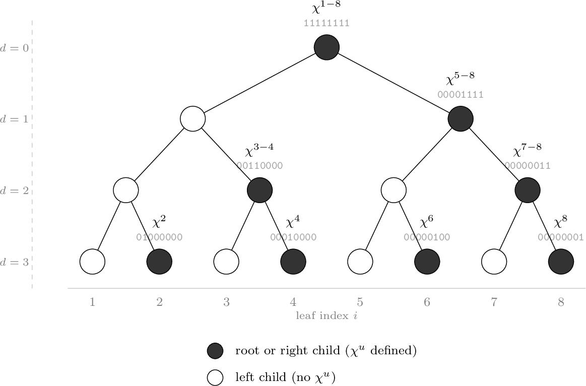
The reason for using this basis is that every suffix vector \(Ae_i\) has a simple representation in it. More precisely, if \(Ae_i\) is the vector with ones in positions \(j \geq i\) and zeros elsewhere, then \[Ae_i = \sum_{u \in \mathcal{I}(i)} \chi^u\] for the set \(\mathcal{I}(i)\) of nodes that are right children of the path to the \(i\)’th leaf from the root (we refer the reader to 4 for the precise statement). Letting \(\mathcal{V}(\mathcal{T}) \subset \mathcal{T}\) be the set of nodes \(u\) with a \(\chi^u\) vector defined (right children and the root), we see that for every input \(x\), we may write \[Ax = \sum_{u \in \mathcal{V}(\mathcal{T})} a_u \chi^u, \qquad a_u = \sum_{i : u \in \mathcal{I}(i)} x_i.\] Similarly, since the \(\chi^u\) vectors form a basis, the noise vector also has a unique expansion \[\mathbf{z}= \sum_{u \in \mathcal{V}(\mathcal{T})} \mathbf{b}_u \chi^u.\] For a leaf \(i\), the released noise in coordinate \(i\) is therefore the sum of the coefficients \(\mathbf{b}_u\) over the nodes \(u\) on the root-to-leaf path to \(i\) for which \(\chi^u\) is defined: \[\mathbf{z}_i = \sum_{u \in \mathop{\mathrm{Anc}}(i) \cap \mathcal{V}(\mathcal{T})} \mathbf{b}_u,\] where \(\mathop{\mathrm{Anc}}(i)\) are the ancestors of the \(i\)’th leaf (including the \(i\)’th leaf). Thus the \(\ell_\infty\) error is controlled by these path sums.
3.0.0.3 Noise Accumulation.
Having established the tree basis, we now turn to the second part of the proof: constructing the adversary. To define the vectors \(\nu^i\) and \(\mathbf{q}\), we need to understand how the noise \(\mathbf{z}\) is distributed across the tree. Specifically, we argue that noise accumulates up the tree when it has “residual uncertainties”, a notion we now formalize.
Consider a node \(u \in \mathcal{T}\), let \(\mathcal{T}^u\) be the subtree rooted at \(u\), and let \(\mathcal{V}(\mathcal{T}^u) = \mathcal{T}^u \cap \mathcal{V}(\mathcal{T})\) be the set of nodes \(v\) in \(\mathcal{T}^u\) with a \(\chi^v\) vector defined. We now consider the accumulation of the noise \(\mathbf{z}_i\) up to node \(u\) defined as \[\mathbf{z}_i^{< u} := \sum_{v \in (\mathcal{V}(\mathcal{T}^u) \setminus \{u\}) \cap \mathop{\mathrm{Anc}}(i)} \mathbf{b}_v.\] Thus \(\mathbf{z}_i^{<u}\) gives the contribution to \(\mathbf{z}_i\) from nodes below \(u\). Our next key idea is to lower bound \(\mathbb{E}[\max_i \mathbf{z}_i - \min_i \mathbf{z}_i]\) rather than \(\mathbb{E}[\|\mathbf{z}\|_\infty]\) directly, avoiding working with absolute values. This is sufficient since \(\|\mathbf{z}\|_\infty\geq (\max_i \mathbf{z}_i - \min_i \mathbf{z}_i)/2\). If \(\mathcal{L}(\mathcal{T}^u)\) denotes the indices of the leaves of \(\mathcal{T}^u\), we may now consider \[\mathop{\mathrm{max}}^{< u}(\mathbf{z}) := \max_{i \in \mathcal{L}(\mathcal{T}^u)} \mathbf{z}_i^{< u}\] and \[\mathop{\mathrm{min}}^{< u}(\mathbf{z}) := \min_{i \in \mathcal{L}(\mathcal{T}^u)} \mathbf{z}^{< u}_i.\] Our main inductive argument is to show that \(\mathbb{E}[\mathop{\mathrm{max}}^{<u}(\mathbf{z})-\mathop{\mathrm{min}}^{<u}(\mathbf{z})]\) increases as we move up the tree towards the root. Finally, for the root \(\rho\), we have \[\mathop{\mathrm{max}}^{<\rho}(\mathbf{z})-\mathop{\mathrm{min}}^{<\rho}(\mathbf{z}) = (\max_i \mathbf{z}_i - \mathbf{b}_\rho)-(\min_i \mathbf{z}_i - \mathbf{b}_\rho) = \max_i \mathbf{z}_i - \min_i \mathbf{z}_i,\] and thus a lower bound on \(\mathbb{E}[\mathop{\mathrm{max}}^{<\rho}(\mathbf{z})-\mathop{\mathrm{min}}^{<\rho}(\mathbf{z}) ]\) directly translates to a lower bound on \(\mathbb{E}[\|\mathbf{z}\|_\infty]\).
Consider now a non-leaf node \(u\) and the range \(\mathop{\mathrm{max}}^{<u}(\mathbf{z})-\mathop{\mathrm{min}}^{<u}(\mathbf{z})\). Let \(\ell(u)\) denote the left child of \(u\) and \(r(u)\) the right child. We see that \[\mathop{\mathrm{max}}^{<u}(\mathbf{z})-\mathop{\mathrm{min}}^{<u}(\mathbf{z}) = \max\{\mathop{\mathrm{max}}^{<\ell(u)}(\mathbf{z}), \mathop{\mathrm{max}}^{<r(u)}(\mathbf{z}) + \mathbf{b}_{r(u)} \} - \min\{\mathop{\mathrm{min}}^{<\ell(u)}(\mathbf{z}), \mathop{\mathrm{min}}^{<r(u)}(\mathbf{z}) + \mathbf{b}_{r(u)} \}.\] This holds since every \(i \in \mathcal{T}^{r(u)}\) has \(r(u)\) as an ancestor (only the right child of \(u\) has a \(\chi\)-vector). Using that \(\max\{a,b\}-\min\{c,d\} = (a-c)/2+(b-d)/2 + |a-b|/2+|c-d|/2\) we get \[\begin{align} \label{eq:recurse} \mathop{\mathrm{max}}^{<u}(\mathbf{z})-\mathop{\mathrm{min}}^{<u}(\mathbf{z}) &= \frac{\mathop{\mathrm{max}}^{<\ell(u)}(\mathbf{z})-\mathop{\mathrm{min}}^{<\ell(u)}(\mathbf{z})}{2}+\frac{\mathop{\mathrm{max}}^{<r(u)}(\mathbf{z})-\mathop{\mathrm{min}}^{<r(u)}(\mathbf{z})}{2} \nonumber \\ &+\frac{\left|\mathop{\mathrm{max}}^{<\ell(u)}(\mathbf{z})-\mathop{\mathrm{max}}^{<r(u)}(\mathbf{z})-\mathbf{b}_{r(u)} \right|}{2}+\frac{\left|\mathop{\mathrm{min}}^{<\ell(u)}(\mathbf{z})-\mathop{\mathrm{min}}^{<r(u)}(\mathbf{z}) - \mathbf{b}_{r(u)} \right|}{2}. \end{align}\tag{1}\] The first line is very convenient as it expresses \(\mathop{\mathrm{max}}^{<u}(\mathbf{z})-\mathop{\mathrm{min}}^{<u}(\mathbf{z})\) recursively as the average of the same quantity in the two children’s subtrees. What remains is thus to argue that the second line introduces a noticeable growth in \(\max^{<u}(\mathbf{z})-\min^{<u}(\mathbf{z})\) as we move up the tree.
Taking expectation on both sides of 1 , we thus need to lower bound \[\begin{align} \mathbb{E}\left[\left|\mathop{\mathrm{max}}^{<\ell(u)}(\mathbf{z})-\mathop{\mathrm{max}}^{<r(u)}(\mathbf{z})-\mathbf{b}_{r(u)} \right|\right], \label{eq:topredict} \end{align}\tag{2}\] and symmetrically for \(\min\). Here our main observation is that \(\mathop{\mathrm{max}}^{<\ell(u)}(\mathbf{z})\) and \(\mathop{\mathrm{max}}^{<r(u)}(\mathbf{z})\) depend only on the noise below \(\ell(u)\) and \(r(u)\). We thus define a type of “residual noise”. Let \(\Delta^{<u}(\mathbf{z})\) denote the random variable giving the noise \(\mathbf{b}_v\) for every \(v\) in the subtree below \(u\) (excluding \(u\)). We now define \(\sigma_{u}\) to capture how well \(\mathbf{b}_{r(u)}\) can be predicted from the noise \(\Delta^{<\ell(u)}(\mathbf{z}), \Delta^{<r(u)}(\mathbf{z})\): \[\sigma_{u}(\Delta^{<\ell(u)}(\mathbf{z}), \Delta^{<r(u)}(\mathbf{z})) := \inf_m \mathbb{E}[|\mathbf{b}_{r(u)}-m| \mid \Delta^{<\ell(u)}(\mathbf{z}), \Delta^{<r(u)}(\mathbf{z})].\]
Returning to 2 and recalling that \(\mathop{\mathrm{max}}^{<\ell(u)}(\mathbf{z})\) and \(\mathop{\mathrm{max}}^{<r(u)}(\mathbf{z})\) depend only on \(\Delta^{<\ell(u)}(\mathbf{z}), \Delta^{<r(u)}(\mathbf{z})\) we thus conclude that 2 is at least \[\begin{align} \sigma_{u} := \mathbb{E}[\sigma_{u}(\Delta^{<\ell(u)}(\mathbf{z}), \Delta^{<r(u)}(\mathbf{z}))]. \end{align}\] We thus get an increase in \(\mathbb{E}[\max^{<u}(\mathbf{z})-\min^{<u}(\mathbf{z})]\) if there is still randomness left in \(\mathbf{b}_{r(u)}\) conditioned on the noise in the subtrees below \(\ell(u)\) and \(r(u)\). In particular, recursively unfolding 1 and letting \(d(u)\) denote the depth of a node \(u \in \mathcal{T}\) with the root \(\rho\) at depth \(0\), we get \[\begin{align} \label{eq:unfolded} \mathbb{E}[\|\mathbf{z}\|_\infty] &\geq \mathbb{E}[\max_i \mathbf{z}_i - \min_i \mathbf{z}_i]/2 \nonumber\\ &= \mathbb{E}[\mathop{\mathrm{max}}^{<\rho}(\mathbf{z}) - \mathop{\mathrm{min}}^{<\rho}(\mathbf{z})]/2 \nonumber\\ &\geq \frac{1}{4} \sum_{d=0}^{h} \sum_{u \in \mathcal{T}: d(u)=d} 2^{-d} \sigma_{u}. \end{align}\tag{3}\] Observe that \(\sum_{d=0}^{h} \sum_{u \in \mathcal{T}: d(u)=d} 2^{-d} \sigma_{u}\) equals the expected sum of \(\sigma_{u}\) values along a uniform random root-to-leaf path in \(\mathcal{T}\).
Before proceeding to explain how we lower bound this sum of \(\sigma_{u}\) values, let us compare to the classic binary tree mechanism upper bound. There, every node in the binary tree adds independent noise of variance \(\Theta(\log n)\). This means that even conditioned on the noise in the subtrees below \(\ell(u)\) and \(r(u)\), we still have \(\mathbb{E}[\inf_m \mathbb{E}[|\mathbf{b}_{r(u)}-m| \mid \Delta^{<\ell(u)}(\mathbf{z}), \Delta^{<r(u)}(\mathbf{z})]] = \Omega(\sqrt{\log n})\). Summing \(\Omega(\sqrt{\log n})\) for each of the \(\log_2 n\) nodes along a root-to-leaf path leads to the claimed \(\Omega(\log^{3/2} n)\) lower bound.
By 3 , our goal reduces to showing that no private mechanism can make do with small residual noise \(\sigma_u\).
3.0.0.4 Obstacles for Bounding Residual Noise via Linear Measurements.
The main obstacle is that the adversary cannot directly compute the subtree noise \(\Delta^{<\ell(u)}(\mathbf{z}), \Delta^{<r(u)}(\mathbf{z})\) needed to predict \(\mathbf{b}_{r(u)}\). To see why, consider the following attempt: let the adversary compute \(\mathbf{x}_i Ae_i + \mathbf{z}\), write it (uniquely) in the basis \(\chi^u\) and thereby obtain, for every node \(u \in \mathcal{V}(\mathcal{T})\), the value \[\mathbf{b}_u + \mathbf{x}_i \mathbb{1}\{u \in \mathcal{I}(i)\}.\] Next, for every non-leaf node \(u \in \mathcal{T}\), if the adversary could compute \(\Delta^{<\ell(u)}(\mathbf{z}), \Delta^{<r(u)}(\mathbf{z})\), they could subtract the conditional median \(m^u(\Delta^{<\ell(u)}(\mathbf{z}), \Delta^{<r(u)}(\mathbf{z}))\), the smallest minimizer of \(\mathbb{E}[|\mathbf{b}_{r(u)} - m | \mid \Delta^{<\ell(u)}(\mathbf{z}), \Delta^{<r(u)}(\mathbf{z})]\) over \(m\), from \(\mathbf{b}_{r(u)} + \mathbf{x}_i \mathbb{1}\{r(u) \in \mathcal{I}(i)\}\), obtaining a residual \(\mathbf{q}_u := \mathbf{b}_{r(u)}- m^u(\Delta^{<\ell(u)}(\mathbf{z}), \Delta^{<r(u)}(\mathbf{z}))\) satisfying \(\mathbb{E}[|\mathbf{q}_u|] = \sigma_{u}\) (see 2 for an illustration). This would produce the desired vector \(\mathbf{x}_i\nu^i + \mathbf{q}\), where both \(\nu^i\) and \(\mathbf{q}\) are indexed over non-leaf nodes \(u \in \mathcal{T}\), with \(\nu^i\) having entries \(\mathbb{1}\{r(u) \in \mathcal{I}(i)\}\).
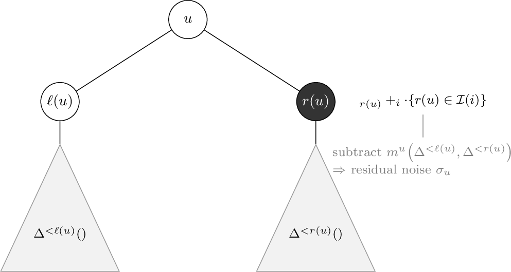
Unfortunately the adversary cannot compute \(\Delta^{<\ell(u)}(\mathbf{z}), \Delta^{<r(u)}(\mathbf{z})\) from \(\mathbf{x}_i A e_i + \mathbf{z}\). The obstacle is that for any node \(v \in \mathcal{I}(i)\) in the subtrees below \(\ell(u)\) or \(r(u)\), the adversary observes \(\mathbf{b}_v+\mathbf{x}_i\) rather than \(\mathbf{b}_v\) alone. Since \(\mathbf{x}_i\) is unknown, the adversary cannot extract the noise \(\mathbf{b}_v\). To remedy this, we take a step back and slightly redefine \(\sigma_{u}\).
3.0.0.5 Noise Prediction via Grandchildren.
Consider again a non-leaf node \(u\) and assume the children of \(u\) are also internal nodes. Instead of arguing that \(\mathop{\mathrm{max}}^{<u}(\mathbf{z})-\mathop{\mathrm{min}}^{<u}(\mathbf{z})\) grows compared to \((\mathop{\mathrm{max}}^{<\ell(u)}(\mathbf{z})-\mathop{\mathrm{min}}^{<\ell(u)}(\mathbf{z}))/2 + (\mathop{\mathrm{max}}^{<r(u)}(\mathbf{z})-\mathop{\mathrm{min}}^{<r(u)}(\mathbf{z}))/2\), we can also relate it to the grandchildren.
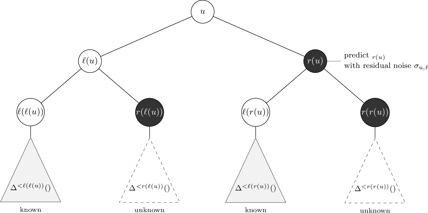
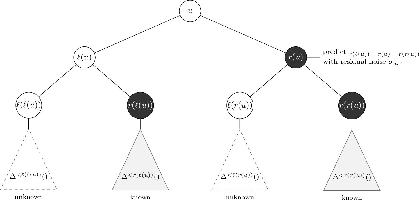
In more detail, consider first the two grandchildren \(\ell(\ell(u))\) and \(\ell(r(u))\) who are both left children of their parent. Since \(\mathop{\mathrm{Anc}}(i)\) for \(i \in \mathcal{L}(\mathcal{T}^{\ell(\ell(u))})\) contains none of \(r(u), r(\ell(u))\) and \(r(r(u))\) (the only nodes among \(u\), the children of \(u\), and the grandchildren, who have a \(\chi\)-vector), we get \(\mathbf{z}^{<u}_i = \mathbf{z}^{<\ell(\ell(u))}_i\). Likewise, \(\mathop{\mathrm{Anc}}(i)\) for \(i \in \mathcal{L}(\mathcal{T}^{\ell(r(u))})\) contains precisely \(r(u)\) and hence, similarly to 1 , we get \[\begin{align} &\mathop{\mathrm{max}}^{<u}(\mathbf{z})-\mathop{\mathrm{min}}^{<u}(\mathbf{z}) \geq \nonumber\\ &\frac{\mathop{\mathrm{max}}^{<\ell(\ell(u))}(\mathbf{z})-\mathop{\mathrm{min}}^{<\ell(\ell(u))}(\mathbf{z})}{2}+\frac{\mathop{\mathrm{max}}^{<\ell(r(u))}(\mathbf{z})-\mathop{\mathrm{min}}^{<\ell(r(u))}(\mathbf{z})}{2} +\nonumber\\ &\frac{\left|\mathop{\mathrm{max}}^{<\ell(\ell(u))}(\mathbf{z})-\mathop{\mathrm{max}}^{<\ell(r(u))}(\mathbf{z})-\mathbf{b}_{r(u)} \right|}{2}+\frac{\left|\mathop{\mathrm{min}}^{<\ell(\ell(u))}(\mathbf{z})-\mathop{\mathrm{min}}^{<\ell(r(u))}(\mathbf{z}) - \mathbf{b}_{r(u)} \right|}{2}.\label{eq:grand1} \end{align}\tag{4}\] We can thus define \(\sigma_{u,\ell}\) to measure the residual noise in \(\mathbf{b}_{r(u)}\) conditioned on the grandchildren \(\ell(\ell(u))\) and \(\ell(r(u))\) (see 3): \[\sigma_{u,\ell} := \mathbb{E}[\inf_m \mathbb{E}[|\mathbf{b}_{r(u)}-m| \mid \Delta^{<\ell(\ell(u))}(\mathbf{z}), \Delta^{<\ell(r(u))}(\mathbf{z})]].\] The symmetric case where we consider the grandchildren \(r(\ell(u))\) and \(r(r(u))\) is slightly more complicated as \(\mathop{\mathrm{Anc}}(i)\) for \(i \in \mathcal{L}(\mathcal{T}^{r(\ell(u))})\) contains \(r(\ell(u))\) and for \(i \in \mathcal{L}(\mathcal{T}^{r(r(u))})\) contains both \(r(u)\) and \(r(r(u))\). This gives \[\begin{align} &\mathop{\mathrm{max}}^{<u}(\mathbf{z})-\mathop{\mathrm{min}}^{<u}(\mathbf{z}) \geq \nonumber\\ &\frac{\mathop{\mathrm{max}}^{<r(\ell(u))}(\mathbf{z})-\mathop{\mathrm{min}}^{<r(\ell(u))}(\mathbf{z})}{2}+\frac{\mathop{\mathrm{max}}^{<r(r(u))}(\mathbf{z})-\mathop{\mathrm{min}}^{<r(r(u))}(\mathbf{z})}{2} + \nonumber\\ &\frac{\left|\mathop{\mathrm{max}}^{<r(\ell(u))}(\mathbf{z})-\mathop{\mathrm{max}}^{<r(r(u))}(\mathbf{z})+\mathbf{b}_{r(\ell(u))}-\mathbf{b}_{r(u)}-\mathbf{b}_{r(r(u))} \right|}{2}+\nonumber \\ &\frac{\left|\mathop{\mathrm{min}}^{<r(\ell(u))}(\mathbf{z})-\mathop{\mathrm{min}}^{<r(r(u))}(\mathbf{z})+\mathbf{b}_{r(\ell(u))}-\mathbf{b}_{r(u)}-\mathbf{b}_{r(r(u))}\right|}{2}. \label{eq:grand2} \end{align}\tag{5}\] We handle this by measuring the residual noise in the sum \(\mathbf{b}_{r(\ell(u))}-\mathbf{b}_{r(u)}-\mathbf{b}_{r(r(u))}\) instead (see 4): \[\sigma_{u,r} := \mathbb{E}[\inf_m \mathbb{E}[|\mathbf{b}_{r(\ell(u))}-\mathbf{b}_{r(u)}-\mathbf{b}_{r(r(u))}-m| \mid \Delta^{<r(\ell(u))}(\mathbf{z}), \Delta^{<r(r(u))}(\mathbf{z})]].\]
Averaging 4 and 5 , we conclude \[\begin{align} &\mathbb{E}[\mathop{\mathrm{max}}^{<u}(\mathbf{z})-\mathop{\mathrm{min}}^{<u}(\mathbf{z})] \geq \sigma_{u,\ell}/2 + \sigma_{u,r}/2 + \sum_{f,g \in \{\ell,r\}} \frac{\mathbb{E}\left[ \mathop{\mathrm{max}}^{<f(g(u))}(\mathbf{z})-\mathop{\mathrm{min}}^{<f(g(u))}(\mathbf{z})\right]}{4}. \end{align}\] Starting from the root, which has depth \(0\), we can recursively unfold this sum and, similarly to 3 , we conclude \[\begin{align} \mathbb{E}[\|\mathbf{z}\|_\infty] = \Omega\left(\sum_{d=0}^{h/2} \sum_{u \in \mathcal{T}: d(u)=2d} 2^{-2d} (\sigma_{u,\ell} + \sigma_{u,r}) \right). \label{eq:evensum} \end{align}\tag{6}\] Note that the sum is again the expectation over a random root-to-leaf path, of the sum of \(\sigma_{u,\ell}\) and \(\sigma_{u,r}\) for nodes \(u\) at even levels of \(\mathcal{T}\).
Now, let us look carefully at what we have gained from predicting the noise from the grandchildren. The key observation is that for an adversary trying to distinguish neighboring \(x',x''\) with \(x'_i \neq x''_i\), it holds for any node \(u\) that if \(i \in \mathcal{L}(\mathcal{T}^{r(\ell(u))}) \cup \mathcal{L}(\mathcal{T}^{r(r(u))})\), then \(v \notin \mathcal{I}(i)\) for all \(v \in \mathcal{T}^{\ell(\ell(u))} \setminus \{\ell(\ell(u))\}\) and all \(v \in \mathcal{T}^{\ell(r(u))} \setminus \{\ell(r(u))\}\). The symmetric thing holds for \(i \in \mathcal{L}(\mathcal{T}^{\ell(\ell(u))}) \cup \mathcal{L}(\mathcal{T}^{\ell(r(u))})\). In a nutshell, if an adversary “attacks” a variable \(\mathbf{x}_i\) with \(i\) in the subtree of one of the two grandchildren \(r(\ell(u))\) and \(r(r(u))\), then the adversary can directly compute \(\Delta^{<\ell(\ell(u))}(\mathbf{z}), \Delta^{<\ell(r(u))}(\mathbf{z})\) and predict \(\mathbf{b}_{r(u)}\) up to an expected absolute error of \(\sigma_{u,\ell}\). A symmetric argument allows the adversary to predict \(\mathbf{b}_{r(\ell(u))}-\mathbf{b}_{r(u)}-\mathbf{b}_{r(r(u))}\) up to expected error \(\sigma_{u,r}\) if \(i\) is in the subtree of either \(\ell(\ell(u))\) or \(\ell(r(u))\). Let us ignore this slightly more tedious case in the proof overview.
Unfortunately, a new obstacle arises from this approach. One central idea in the linear measurements approach for bounding the noise, is to define orthogonal unit length vectors \(\psi^i\) so that \(\sum_i \mathbb{E}[\langle \psi^i, \mathbf{z}\rangle^2] \leq \mathbb{E}[\|\mathbf{z}\|_2^2]\). Now, if we follow the outlined approach and use the noise in the pair of grandchildren not containing the \(i\)’th leaf, then the distribution of the residual noise vector \(\mathbf{q}\) depends on \(i\). That is, if \(i\) falls in one of the subtrees rooted at the grandchildren \(\ell(\ell(u)), \ell(r(u))\), we get one distribution, and if it falls in the subtrees rooted at \(r(\ell(u)), r(r(u))\), we get another. If we have different residual noise vectors \(\mathbf{q}^i\) for different \(i\), then the argument \(\sum_i \mathbb{E}[\langle \psi^i, \mathbf{q}^i \rangle^2] \leq \mathbb{E}[\|\mathbf{q}\|_2^2]\) breaks, since \(\mathbf{q}\) is not a fixed vector as it depends on \(i\).
3.0.0.6 Restricting to a Subtree.
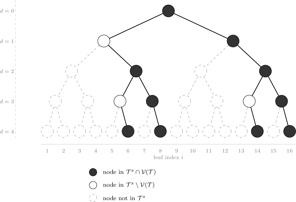
Our next idea is to restrict attention to a collection of leaf indices \(i\) that all result in the same noise predictions across the tree \(\mathcal{T}\). In more detail, consider a string \(s \in \{\ell,r\}^{h/2}\) and let \(\mathcal{T}^s\) be the subset of \(\mathcal{T}\) defined as follows. Starting from the root, from a node at an even depth \(2d\) we descend into both children, and from a node at an odd depth \(2d-1\) we descend only to the left child if \(s_d=\ell\) and only to the right child if \(s_d=r\). Let \(\mathcal{L}(\mathcal{T}^s)\) be the indices of the leaves of \(\mathcal{T}^s\).
The critical observation is that if \(u \in \mathcal{T}^s\) is a node of even depth \(2d\), then every \(i \in \mathcal{L}(\mathcal{T}^s) \cap \mathcal{L}(\mathcal{T}^u)\) falls in one of the two subtrees \(\mathcal{T}^{s_{d+1}(\ell(u))}\) and \(\mathcal{T}^{s_{d+1}(r(u))}\). This implies that an adversary trying to infer \(\mathbf{x}_i\) via a linear measurement can compute \(\Delta^{<\widetilde{s_{d+1}}(\ell(u))}(\mathbf{z}), \Delta^{<\widetilde{s_{d+1}}(r(u))}(\mathbf{z})\) regardless of which \(i \in \mathcal{L}(\mathcal{T}^s)\) the adversary attacks, where \(\widetilde{\ell} = r\) and \(\widetilde{r} = \ell\) denotes the opposite direction. The adversary can thus predict \(\mathbf{b}_{r(u)}\) up to expected absolute error \(\sigma_{u,\ell}\) if \(s_{d+1}=r\), and predict \(\mathbf{b}_{r(\ell(u))}-\mathbf{b}_{r(u)}-\mathbf{b}_{r(r(u))}\) up to error \(\sigma_{u,r}\) if \(s_{d+1}=\ell\).
Assume for simplicity that \(s = r r \cdots r\) is the all-r string, so we do not have to deal with the \(\mathbf{b}_{r(\ell(u))}-\mathbf{b}_{r(u)}-\mathbf{b}_{r(r(u))}\) case. For a neighboring pair \(x',x''\) with \(x'_i \neq x''_i\) and \(\mathbf{x}\) uniform in \(\{x',x''\}\), an adversary can now compute \[\mathbf{b}_{r(u)}+ \mathbf{x}_i \mathbb{1}\{r(u) \in \mathcal{I}(i)\} - m^u_\ell(\Delta^{<\ell(\ell(u))}(\mathbf{z}), \Delta^{<\ell(r(u))}(\mathbf{z}))= \mathbf{q}_u + \mathbf{x}_i \mathbb{1}\{r(u) \in \mathcal{I}(i)\}\] for every \(u \in \mathcal{T}^s\) of even depth, where \(\mathbb{E}[|\mathbf{q}_u|] = \sigma_{u,\ell}\). Here \(m^u_\ell\) is a conditional median of \(\mathbf{b}_{r(u)}\).
Letting \(\nu^i\) be the vector with entries \(\mathbb{1}\{r(u) \in \mathcal{I}(i)\}\) for every \(u \in \mathcal{T}^s\) of even depth, the adversary has thus obtained a vector \(\mathbf{x}_i \nu^i + \mathbf{q}\) with \(\mathbb{E}[|\mathbf{q}_u|] = \sigma_{u,\ell}\). Moreover, if we draw \(\mathbf{s}\) uniformly in \(\{\ell,r\}^{h/2}\), then a uniform random root-to-leaf path in \(\mathcal{T}^{\mathbf{s}}\), is uniform random in \(\mathcal{T}\). Thus if we can lower bound the expected sum of \(\sigma_{u,\ell} + \sigma_{u,r}\) along a uniform random root-to-leaf path in every \(\mathcal{T}^s\), then we get the same lower bound on 6 . We thus fix an arbitrary \(s \in \{\ell,r\}^{h/2}\) and lower bound \[\begin{align} \label{eq:ts} \sum_{d=0}^{h/2} \sum_{u \in \mathcal{T}^s : d(u)=2d} 2^{-d} \sigma_{u,\widetilde{s_{d+1}}}. \end{align}\tag{7}\] For simplicity of the proof overview, let us merely consider \(s=rr \cdots r\) and \(\sum_{d=0}^{h/2} \sum_{u \in \mathcal{T}^s : d(u)=2d} 2^{-d} \sigma_{u,\ell}\). See 5 for an example for \(n=16\) and \(s=rr\).
3.0.0.7 Median-of-Three Trick.
We now have an adversary for every \(i \in \mathcal{L}(\mathcal{T}^s)\) that can compute \(\mathbf{x}_i \nu^i + \mathbf{q}\). Returning to the strategy of using linear measurements, the natural next step would be to define orthogonal unit length vectors \(\psi^i\) for which \(\sum_i \langle \psi^i, \nu^i\rangle^2\) is large. By orthogonality, we would simultaneously get \(\sum_i \mathbb{E}[\langle \psi^i, \mathbf{q}\rangle^2] \leq \mathbb{E}[\|\mathbf{q}\|_2^2] = \sum_{u \in \mathcal{T}^s: d(u) \textrm{ even}} \mathbb{E}[\mathbf{q}_u^2]\). Unfortunately, our guarantee \(\mathbb{E}[|\mathbf{q}_u|] = \sigma_{u,\ell}\) is not sufficient to give any upper bound on \(\mathbb{E}[ \mathbf{q}_u^2]\) and thereby \(\mathbb{E}[\|\mathbf{q}\|_2^2]\). To overcome this, we use a trick from Larsen, Pagh, Tetek [29]. An immediate corollary of their work is the following.
Corollary 1 ([29]). Let \(\mathbf{Z}_1,\mathbf{Z}_2,\mathbf{Z}_3\) be i.i.d.real-valued random variables. Then \[\mathbb{E}[\mathop{\mathrm{median}}\{\mathbf{Z}_1,\mathbf{Z}_2,\mathbf{Z}_3\}^2] \leq 3 \cdot \mathbb{E}[|\mathbf{Z}_1|]^2.\]
Now using the composition property of differential privacy, we have that the mechanism \(\mathbf{M}'\) releasing \((Ax+\mathbf{z}^{(1)}, Ax+\mathbf{z}^{(2)}, Ax+\mathbf{z}^{(3)})\) for three i.i.d.draws of the noise \(\mathbf{z}\) of the mechanism \(\mathbf{M}\) is \((3\varepsilon, 3\delta)\)-DP. Thus even if we give an adversary access to three independent copies of the noise, privacy still guarantees that one cannot distinguish \(x', x''\). Crucially, the adversary trying to infer \(\mathbf{x}_i\) can now compute, for every \(u \in \mathcal{T}^s\) of even depth, the value \[\begin{align} &\mathop{\mathrm{median}}\{\mathbf{x}_i \mathbb{1}\{r(u) \in \mathcal{I}(i)\} + \mathbf{q}_u^{(1)},\mathbf{x}_i \mathbb{1}\{r(u) \in \mathcal{I}(i)\} + \mathbf{q}_u^{(2)},\mathbf{x}_i \mathbb{1}\{r(u) \in \mathcal{I}(i)\} + \mathbf{q}_u^{(3)}\} =\\ & \mathbf{x}_i \mathbb{1}\{r(u) \in \mathcal{I}(i)\} + \mathop{\mathrm{median}}\{ \mathbf{q}_u^{(1)}, \mathbf{q}_u^{(2)}, \mathbf{q}_u^{(3)}\}. \end{align}\] From Corollary 1, this results in a vector \(\mathbf{x}_i \nu^i + \mathbf{q}\) where \[\mathbb{E}[(\mathbf{q}_u)^2] = \mathbb{E}[\mathop{\mathrm{median}}\{ \mathbf{q}_u^{(1)}, \mathbf{q}_u^{(2)}, \mathbf{q}_u^{(3)}\}^2] \leq 3 \mathbb{E}[|\mathbf{q}_u^{(1)}|]^2 = 3 \sigma_{u,\ell}^2.\] We thus have \[\begin{align} \mathbb{E}[\|\mathbf{q}\|_2^2] \leq 3 \sum_{d=0}^{h/2} \sum_{u \in \mathcal{T}^s : d(u)=2d} \sigma^2_{u,\ell}. \label{eq:sumsquare} \end{align}\tag{8}\] As suggested earlier, the next step is to define the linear measurements \(\psi^i\) and then use privacy to argue that \(\mathbb{E}[\|\mathbf{q}\|_2^2] = \Omega(\sum_i \langle \psi^i, \nu^i\rangle^2)\). Indeed this would lower bound the sum of \(\sigma^2_{u,\ell}\). Sadly, this is not enough as we need to bound the weighted sum of \(\sigma_{u,\ell}\) given in 7 . We thus have a mismatch, both in terms of weights, but more critically, 8 is a sum of squares whereas 7 is a sum.
Let us mention that our full proof handles the above in a slightly different manner. Rather than attacking different \(\mathbf{x}_i\) variables directly, we separate the noise reduction step from the linear measurement attacks, making the proof more modular. In essence, we define a derived mechanism \(\widehat{\mathbf{M}}\) that is \((3\varepsilon, 3\delta)\)-DP when restricted to inputs with \(x_i = 0\) for \(i \notin \mathcal{L}(\mathcal{T}^s)\), and apply the linear measurements argument to \(\widehat{\mathbf{M}}\). Since \(|\mathcal{L}(\mathcal{T}^s)| = \sqrt{n}\) and the lower bound is polylogarithmic, the restriction to a smaller input domain is harmless.
3.0.0.8 From Weighted Sum to Max Bound.
We now address the mismatch between the sum of squares in 8 and the weighted sum 7 that we need to lower bound. We will show that for at least half of the \(h/2\) choices of depth \(2d\), at least half of the nodes \(u \in \mathcal{T}^s\) must have \(\sigma_{u,\ell} = \Omega(\sqrt{\log n})\). This still lower bounds 7 by the desired \(\Omega(\log^{3/2} n)\).
The way we approach it is as follows: for every even depth \(2d\), consider the median \[m_d := \mathop{\mathrm{median}}_{u \in \mathcal{T}^s : d(u)=2d} \{\sigma_{u,\ell}\}.\] Now let \(\mathcal{J}\subseteq \{0,\dots,h/2-1\}\) with \(|\mathcal{J}|=h/4\) be so that the medians \(m_d\) with \(d \in \mathcal{J}\) are the \(h/4\) smallest of the \(h/2\) medians. Furthermore, for every \(d \in \mathcal{J}\), let \(\mathcal{J}_d\) consist of the nodes \(u \in \mathcal{T}^s\) of depth \(2d\) having the smallest \(\sigma_{u,\ell}\) values. In particular, each such \(\sigma_{u,\ell}\) satisfies \(\sigma_{u,\ell} \leq m_d\). Let us now define \[\sigma := \max_{d \in \mathcal{J}} \max_{u \in \mathcal{J}_d} \sigma_{u,\ell}.\] Then by definition of \(\mathcal{J}\), for each of the \(h/4\) values of \(d\) not in \(\mathcal{J}\), we have \(m_d \geq \sigma\). Hence, at least half the nodes of depth \(2d\) have \(\sigma_{u,\ell} \geq \sigma\). Summing across the \(h/4\) depths not in \(\mathcal{J}\), we lower bound 7 by \[\begin{align} \label{eq:fullsum} &\sum_{d=0}^{h/2} \sum_{u \in \mathcal{T}^s : d(u)=2d} 2^{-d} \sigma_{u,\ell} \geq \sum_{d \notin \mathcal{J}} \sum_{u \in \mathcal{T}^s : d(u)=2d \wedge \sigma_{u,\ell} \geq m_d} 2^{-d} m_d \geq \sum_{d \notin \mathcal{J}} 2^{d-1} 2^{-d} \sigma = \sum_{d \notin \mathcal{J}} \sigma/2 = h\sigma /8. \end{align}\tag{9}\] With this in mind, we now set out to prove that for any choice of \(\mathcal{J}\subseteq \{0,\dots,h/2-1\}\) with \(|\mathcal{J}|=h/4\) and any choice of \(\{\mathcal{J}_d\}_{d \in \mathcal{J}}\) with \(\mathcal{J}_d\) containing half the nodes in \(\mathcal{T}^s\) of depth \(2d\), there is at least one node \(u \in \cup_{d \in \mathcal{J}} \mathcal{J}_d\) with \(\sigma_{u,\ell} = \Omega(\sqrt{\log n})\).
What we have achieved is that we now need to handle the simpler task of showing that just one residual noise must be large, rather than showing that an intricate weighted sum is large. Furthermore, showing that just one \(\sigma_{u,\ell}\) is large is also possible when given a lower bound on the sum of squared values, as in 8 , making the attacks via linear measurements amenable.
3.0.0.9 Privacy Attacks via Linear Measurements.
We now describe the second part of the proof: constructing the adversary using linear measurements. Having analyzed the noise structure in the tree, we have shown that the noise of mechanism \(\mathbf{M}\) has residual contributions \(\sigma_{u,\ell}\) along the tree. It remains to show that if these residual contributions are small, then privacy is violated. Recall that for simplicity we consider \(s=rr\ldots r\) and an adversary trying to distinguish neighboring inputs \(x', x''\) with \(x_i'\neq x_i''\) for some \(i \in \mathcal{L}(\mathcal{T}^s)\). As shown above, this adversary can compute a vector \(\mathbf{x}_i \nu^i + \mathbf{q}\) with an entry for each non-leaf \(u \in \mathcal{T}^s\) of even depth so that \(\mathbb{E}[\mathbf{q}_u^2] \leq 3 \sigma_{u,\ell}^2\) and \(\nu^i_u = \mathbb{1}\{r(u) \in \mathcal{I}(i) \}\). We now show that if the \(\sigma_{u,\ell}\) are small, the adversary can use linear measurements to distinguish \(x'\) from \(x''\), contradicting privacy.
Recall from above the arbitrary sets \(\mathcal{J}\subseteq \{0,\dots,h/2-1\}\) with \(|\mathcal{J}|=h/4\) and \(\{\mathcal{J}_d\}_{d \in \mathcal{J}}\) with \(\mathcal{J}_d\) containing half the nodes in \(\mathcal{T}^s\) of depth \(2d\). We need to define \(\psi^i\) (specified shortly) with the goal of showing that at least one \(\sigma_{u,\ell}\) for \(u \in \cup_{d \in \mathcal{J}} \mathcal{J}_d\) is large. Since post-processing preserves privacy, the adversary may set all coordinates corresponding to \(u \notin \cup_{d \in \mathcal{J}} \mathcal{J}_d\) to \(0\), obtaining a shorter vector. It now suffices to show that \(\mathbb{E}[\mathbf{q}_u^2]\) is large for at least one remaining coordinate \(u\), which by \(\mathbb{E}[\mathbf{q}_u^2]\leq 3 \sigma^2_{u,\ell}\) implies that \(\sigma_{u,\ell}\) is large. Let \(\sigma = \max_{d \in \mathcal{J}} \max_{u \in \mathcal{J}_d} \sigma_{u,\ell}\). Then by definition, \(\mathbb{E}[\|\mathbf{q}\|_2^2] \leq \sum_{d \in \mathcal{J}} \sum_{u \in \mathcal{J}_d} 3 \sigma^2\). Since \(\mathcal{T}^s\) has \(2^d\) nodes at even depth \(2d\) and \(\mathcal{J}_d\) contains half of them, we have \(|\mathcal{J}_d|=2^{d-1}\), meaning deeper levels contribute more to the sum. To balance this across depths, the adversary scales each coordinate of \(\mathbf{x}_i \nu^i + \mathbf{q}\) by \(2^{-d/2}\) for nodes \(u\) at even depth \(2d\). Let \(\mathbf{r}\) be the resulting noise vector with \(\mathbf{r}_u = 2^{-d/2} \mathbf{q}_u\) for \(u \in \cup_{d \in \mathcal{J}} \mathcal{J}_d\) and let \(\mu^i\) be the vector with coordinates \(\mu^i_u = 2^{-d/2} \nu^i_u\). The adversary has thus computed the vector \(\mathbf{x}_i \mu^i + \mathbf{r}\). With \(\psi^i\) as the linear measurement for leaf index \(i\), the adversary computes the estimate \[\hat{\mathbf{x}}_i = \frac{\langle \psi^i, \mathbf{x}_i\mu^i+\mathbf{r}\rangle}{\langle \psi^i, \mu^i\rangle} = \mathbf{x}_i+\frac{\langle \psi^i, \mathbf{r}\rangle}{\langle \psi^i, \mu^i\rangle}.\]
Since \(\hat{\mathbf{x}}_i\) is a private estimate of the binary variable \(\mathbf{x}_i\), applying 1 the error of the adversary for coordinate \(i\) is \[\frac{\mathbb{E}[\langle \psi^i, \mathbf{r}\rangle^2]}{\langle \psi^i, \mu^i\rangle^2} = \Omega(\min\{\varepsilon^{-2}, \delta^{-2}\}).\]
If we choose orthogonal unit length vectors \(\psi^i\) for \(i \in \mathcal{L}(\mathcal{T}^s)\), then \(\sum_{i \in \mathcal{L}(\mathcal{T}^s)} \mathbb{E}[\langle \psi^i, \mathbf{r}\rangle^2 ] \leq E[\|\mathbf{r}\|_2^2]\) and \[\begin{align} E[\|\mathbf{r}\|_2^2] &= \sum_{d \in \mathcal{J}} \sum_{u \in \mathcal{J}_d} \mathbb{E}[\mathbf{r}_u^2]= \sum_{d \in \mathcal{J}} \sum_{u \in \mathcal{J}_d} 2^{-d} \mathbb{E}[\mathbf{q}_u^2] \\ &\leq \sum_{d \in \mathcal{J}} \sum_{u \in \mathcal{J}_d} 2^{-d} 3 \sigma^2 = O(h \sigma^2) \end{align}\] since \(\sum_{d\in \mathcal{J}} |\mathcal{J}_d|\cdot 2^{-d} = |\mathcal{J}|/2 = h/8\).
The final step of the proof is now to choose appropriate vectors \(\psi^i\) so that \(\sum_i \langle \psi^i , \mu^i \rangle^2\) is large. The choice of \(\psi^i\) is inspired by the Haar wavelet basis. Given a perfect binary tree over \(n\) leaves, the Haar wavelet basis has a vector \(h^u\) for each internal node \(u \in \mathcal{T}\). If the subtree rooted at \(u\) has \(n_u\) leaves, then the vector \(h^u\) has coordinates \(-1/\sqrt{n_u}\) for leaves in the subtree rooted at \(\ell(u)\) and it has coordinates \(1/\sqrt{n_u}\) for leaves in the subtree rooted at \(r(u)\). Finally, the basis also contains the vector with all coordinates \(1/\sqrt{n}\). The Haar wavelet basis is an orthonormal basis of \(\mathbb{R}^n\). If we now arrange the vectors \(h^u\) as columns of a matrix \(H\) and compute its transpose \(H^t\), then the resulting matrix is also orthonormal. More precisely, we use as \(\psi^i\) the columns of \(H^t\), where \(H\) is the matrix of the Haar wavelet basis restricted to \(\mathcal{T}^s\).
Concretely, we let \(\psi^i\) be the vector with one coordinate for every \(u \in \mathcal{T}^s\). For a node \(u\) of depth \(2d\), we let \(\psi^i_u = 0\) if \(i \notin \mathcal{L}(\mathcal{T}^u)\), \(\psi^i_u = -2^{-(h/2-d)/2}\) if \(i \in \mathcal{L}(\mathcal{T}^{\ell(u)})\) and \(\psi^i_u = 2^{-(h/2-d)/2}\) if \(i \in \mathcal{L}(\mathcal{T}^{r(u)})\). Since \(2^{h/2-d}\) is the number of leaves in \(\mathcal{L}(\mathcal{T}^s) \cap \mathcal{L}(\mathcal{T}^u)\), this coincides with the transpose of the matrix \(H\) resulting from the Haar wavelet basis on \(\mathcal{T}^s\). We expand \(\sum_i \langle \psi^i, \mu^i \rangle^2\) and show that the sum is lower bounded by \(\Omega(h^2)\).
Combining the bound \(\sum_i \mathbb{E}[\langle \psi^i, \mathbf{r}\rangle^2] = O(h \sigma^2)\) from above with \(\sum_i \langle \psi^i, \mu^i \rangle^2 = \Omega(h^2)\), implies that \(\sigma^2 = \Omega(h \min\{\varepsilon^{-2},\delta^{-2}\})\). Substituting into 9 finally gives us \[\mathbb{E}[\|\mathbf{z}\|_\infty] = \Omega\left(\sum_{d=0}^{h/2} \sum_{u \in \mathcal{T}^s : d(u)=2d} 2^{-d} \sigma_{u,\ell}\right) = \Omega(h \sigma) = \Omega\left(\frac{h^{3/2}}{\max\{\varepsilon,\delta\}}\right) = \Omega\left(\frac{\log^{3/2} n}{\max\{\varepsilon, \delta\}}\right).\]
4 Formal Lower Bound Proof↩︎
We restate our main result for convenience. For any \(0 < \varepsilon< 1\), \(0 < \delta < C\) for a sufficiently small constant \(C>0\), it holds that any \((\varepsilon,\delta)\)-DP mechanism \(\mathbf{M}\) for continual counting has error \[\max_{x \in \{0,1\}^n }\mathbb{E}[\|\mathbf{M}(x)-Ax\|_\infty] = \Omega\left(\frac{\log^{3/2} n }{\max\{\varepsilon,\delta\}}\right),\] where \(A\) is the \(n \times n\) prefix-sum matrix.
We now prove 1. Our goal is to lower bound the noise needed to release a private version of \(Ax\) for a binary vector \(x \in \{0,1\}^n\). By a reduction in prior works [14], we can assume that a mechanism \(\mathbf{M}_o(x)\) releases \(Ax+\mathbf{z}\) for a noise vector \(\mathbf{z}\) independent of \(x\). Concretely, an \((\varepsilon,\delta)\)-DP data dependent mechanism (\(\mathbf{M}(x)\) may depend on \(x\)) can be made oblivious (\(\mathbf{M}_o(x)=Ax+\mathbf{z}\) for \(\mathbf{z}\) independent of \(x\)) at the cost of scaling \(\varepsilon\) to \(2 \varepsilon\) and \(\delta\) to \(e^\varepsilon\delta\). For the parameter range \(0 < \varepsilon< 1\), this is a constant scaling in the parameters and disappears in the \(\Omega(\cdot)\) notation. Essentially, if \(\mathbf{M}\) is an \((\varepsilon, \delta)\)-DP mechanism with error \(\max_{x \in \{0,1\}^n }\mathbb{E}[\|\mathbf{M}(x)-Ax\|_\infty]\), then there exists an oblivious mechanism \(\mathbf{M}_o\) that is \((2\varepsilon, e\delta)\)-DP with error \[\begin{align} \label{eq:error} \max_{x \in \{0,1\}^n }\mathbb{E}[\|\mathbf{M}(x)-Ax\|_\infty] \geq \max_{x \in \{0,1\}^n }\mathbb{E}[\|\mathbf{M}_o(x)-Ax\|_\infty] = \mathbb{E}[\|\mathbf{z}\|_\infty] . \end{align}\tag{10}\]
4.0.0.1 Tree Structure.
We assume \(n\) is a power of \(16\) and let \(h = \log_2 n\). This only affects the lower bound by a constant factor as we can use the length \(16^{\lfloor \log_{16} n \rfloor}\) prefix of \(x\) to embed the hard instance. To define a basis for \(\mathbb{R}^{n}\), consider a binary tree \(\mathcal{T}\) of height \(h\), i.e.\(\mathcal{T}\) has \(n\) leaves, where the \(i\)-th leaf corresponds to the \(i\)-th coordinate of \(Ax+\mathbf{z}\). Let \(\mathcal{V}(\mathcal{T})\) be the set of nodes that are either the root or the right child of their parent. We use the notation \(\ell(u)\) to denote the left child and \(r(u)\) to denote the right child of a non-leaf node \(u\). For each node \(u \in \mathcal{V}(\mathcal{T})\), we define \(\chi^u\) as the indicator vector having a \(1\) in coordinates corresponding to the leaves in the subtree \(\mathcal{T}^u\) rooted at \(u\) and \(0\) elsewhere. We also define \(\mathcal{V}(\mathcal{T}^u) := \mathcal{V}(\mathcal{T}) \cap \mathcal{T}^u\) as the nodes \(v \in \mathcal{T}^u\) with \(\chi^v\) defined.
We observe that the number of vectors \(|\mathcal{V}(\mathcal{T})| = 1 + \sum_{d =1}^{h} 2^{d-1} = n\). Furthermore, we claim that every suffix vector \(Ae_i \in \mathbb{R}^n\) having a \(1\) in positions \(j \geq i\) and \(0\) elsewhere can be written as a linear combination of the \(\chi^u\) vectors. Since the suffix vectors span \(\mathbb{R}^n\), we conclude that the \(\chi^u\) vectors span \(\mathbb{R}^n\). Moreover, since there are \(n\) of them, they form a basis (although neither orthogonal nor unit length).
To write \(Ae_i\) as a linear combination of the \(\chi^u\) vectors, initialize \(\hat{y}=0\) and traverse the path from the root to the \(i\)’th leaf. For each node \(u\) visited, if \(i\) is the left-most leaf in the subtree \(\mathcal{T}^u\), add \(\chi^u\) to \(\hat{y}\) and terminate. Otherwise, if \(u\) is an internal node and the path descends to \(\ell(u)\), add \(\chi^{r(u)}\) to \(\hat{y}\). Upon termination, we have \(\hat{y} = Ae_i\). Define \(\mathcal{I}(i) \subseteq \mathcal{V}(\mathcal{T})\) as the nodes such that \(Ae_i=\sum_{u \in \mathcal{I}(i)} \chi^{u}\).
We observe that \[\begin{align} Ax = \sum_{i=1}^n x_i Ae_ i = \sum_{i=1}^n \sum_{u \in \mathcal{I}(i)} x_i\chi^{u} = \sum_{u \in \mathcal{V}(\mathcal{T})} \sum_{i : u \in \mathcal{I}(i)} x_i\chi^{u}. \end{align}\] Thus, if we define \[a_u := \sum_{i : u \in \mathcal{I}(i)} x_i,\] then \(Ax = \sum_{u \in \mathcal{V}(\mathcal{T})} a_u \chi^{u}\). We note that since the \(\chi^u\) vectors form a basis, this linear combination is unique.
Since the \(\chi^u\) vectors form a basis, there is also a unique linear combination so that \(\mathbf{z}= \sum_{u \in \mathcal{V}(\mathcal{T})} \mathbf{b}_u \chi^{u}\) with \(\mathbf{b}_u \in \mathbb{R}\). From this it also follows that \[\mathbf{z}_i = \sum_{u \in \mathcal{V}(\mathcal{T}) } \mathbf{b}_u \chi^{u}_i = \sum_{u \in \mathcal{V}(\mathcal{T}) : \chi^{u}_i=1} \mathbf{b}_u.\] Note that the nodes \(u\) with \(\chi^{u}_i=1\) are precisely \(\mathop{\mathrm{Anc}}(i) \cap \mathcal{V}(\mathcal{T})\), where \(\mathop{\mathrm{Anc}}(i)\) is the set of all ancestors of the \(i\)’th leaf, including the leaf itself. Thus, to lower bound \(\|\mathbf{z}\|_\infty\) we need to show that there is an index \(i\) for which \(\sum_{u \in \mathop{\mathrm{Anc}}(i) \cap \mathcal{V}(\mathcal{T})} \mathbf{b}_u\) is large in absolute value.
4.0.0.2 Noise Accumulation.
We next argue that noise accumulates up the tree \(\mathcal{T}\) in a subtle manner. First observe that \(\|\mathbf{z}\|_\infty \geq (\max_i \mathbf{z}_i - \min_i \mathbf{z}_i)/2\). We thus lower bound \(\mathbb{E}[\max_i \mathbf{z}_i - \min_i \mathbf{z}_i]\) instead of directly lower bounding \(\mathbb{E}[\|\mathbf{z}\|_\infty]\), circumventing the absolute value. We do this inductively up the tree \(\mathcal{T}\). For any node \(u \in \mathcal{T}\), let \(\mathcal{T}^u\) be the subtree rooted at \(u\) and define \(\mathcal{L}(\mathcal{T}^u)\) as the indices of the leaves in the subtree rooted at \(u\). For each \(i \in \mathcal{L}(\mathcal{T}^u)\), define \[\mathbf{z}^{< u}_i := \sum_{v \in (\mathcal{V}(\mathcal{T}^u )\setminus \{u\}) \cap \mathop{\mathrm{Anc}}(i)} \mathbf{b}_v.\] That is, \(\mathbf{z}^{< u}_i\) sums only the contributions to \(\mathbf{z}_i\) from nodes strictly below \(u\) on the path from the root to the \(i\)’th leaf. Also define \[\mathop{\mathrm{max}}^{< u}(\mathbf{z}) := \max_{i \in \mathcal{L}(\mathcal{T}^u)} \mathbf{z}_i^{< u}.\] and \[\mathop{\mathrm{min}}^{< u}(\mathbf{z}) := \min_{i \in \mathcal{L}(\mathcal{T}^u)} \mathbf{z}^{< u}_i.\] We will show that \(\mathop{\mathrm{max}}^{< u}(\mathbf{z})-\mathop{\mathrm{min}}^{< u}(\mathbf{z})\) grows as we move up the tree.
For any node \(u \in \mathcal{T}\), define \(\Delta^{<u}(\mathbf{z})\) as the random variable giving \(\mathbf{b}_v\) for every \(v \in \mathcal{V}(\mathcal{T}^u) \setminus \{u\}\). That is, \(\Delta^{<u}(\mathbf{z})\) gives the contributions to the noise vector \(\mathbf{z}\) from \(\chi^v\) vectors in the subtree rooted at \(u\), excluding \(u\) itself. \(\Delta^{<u}(\mathbf{z})\) is thus a function of \(\mathbf{z}\), \(\Delta^{<u}(\mathbf{z}): \mathcal{V}(\mathcal{T}^u) \setminus \{u\} \to \mathbb{R}\) with \(\Delta^{<u}(\mathbf{z})(v) = \mathbf{b}_v\) for \(v \in \mathcal{V}(\mathcal{T}^u) \setminus \{u\}\).
We now consider how well \(\mathbf{b}_{r(u)}\) can be predicted from the noise \(\Delta^{<\ell(\ell(u))}(\mathbf{z}), \Delta^{<\ell(r(u))}(\mathbf{z})\) for \(u \in \mathcal{T}\) that is not a leaf: \[\sigma_{u,\ell}(\Delta^{<\ell(\ell(u))}(\mathbf{z}), \Delta^{<\ell(r(u))}(\mathbf{z})) := \inf_m \mathbb{E}\left[\left|\mathbf{b}_{r(u)} - m\right| \mid \Delta^{<\ell(\ell(u))}(\mathbf{z}), \Delta^{<\ell(r(u))}(\mathbf{z})\right].\] Also let \[\sigma_{u,\ell} = \mathbb{E}[\sigma_{u,\ell}(\Delta^{<\ell(\ell(u))}(\mathbf{z}), \Delta^{<\ell(r(u))}(\mathbf{z}))].\] For later use, we also define \(m_\ell^u(\Delta^{<\ell(\ell(u))}(\mathbf{z}), \Delta^{<\ell(r(u))}(\mathbf{z}))\) as a measurable minimizer \(m\) of \[\inf_m \mathbb{E}\left[\left|\mathbf{b}_{r(u)} - m\right| \mid \Delta^{<\ell(\ell(u))}(\mathbf{z}), \Delta^{<\ell(r(u))}(\mathbf{z})\right],\] chosen as the smallest conditional median.
Similarly, we also consider predicting the sum \(\mathbf{b}_{r(\ell(u))} -\mathbf{b}_{r(u)} - \mathbf{b}_{r(r(u))}\) from \(\Delta^{<r(\ell(u))}(\mathbf{z}), \Delta^{<r(r(u))}(\mathbf{z})\) for internal \(u \in \mathcal{T}\) whose children are not leaves: \[\sigma_{u,r}(\Delta^{<r(\ell(u))}(\mathbf{z}), \Delta^{<r(r(u))}(\mathbf{z})) := \inf_m \mathbb{E}\left[\left|\mathbf{b}_{r(\ell(u))} - \mathbf{b}_{r(u)} - \mathbf{b}_{r(r(u))} - m\right| \mid \Delta^{<r(\ell(u))}(\mathbf{z}), \Delta^{<r(r(u))}(\mathbf{z})\right],\] and let \[\sigma_{u,r} = \mathbb{E}[\sigma_{u,r}(\Delta^{<r(\ell(u))}(\mathbf{z}), \Delta^{<r(r(u))}(\mathbf{z}))].\] Again, we also define \(m^u_r(\Delta^{<r(\ell(u))}(\mathbf{z}), \Delta^{<r(r(u))}(\mathbf{z}))\) as a measurable minimizer of \[\inf_m \mathbb{E}\left[\left|\mathbf{b}_{r(\ell(u))} - \mathbf{b}_{r(u)} - \mathbf{b}_{r(r(u))} - m\right| \mid \Delta^{<r(\ell(u))}(\mathbf{z}), \Delta^{<r(r(u))}(\mathbf{z})\right],\] chosen as the smallest conditional median. Our goal is to show that \(\mathop{\mathrm{max}}^{< u}(\mathbf{z}) - \mathop{\mathrm{min}}^{< u}(\mathbf{z})\) grows proportionally to \(\sigma_{u,r}\) and \(\sigma_{u,\ell}\). Intuitively, this means that if there is still randomness left in \(\mathbf{b}_{r(u)}\) after revealing \(\Delta^{<\ell(\ell(u))}(\mathbf{z}), \Delta^{<\ell(r(u))}(\mathbf{z})\), or in \(\mathbf{b}_{r(\ell(u))} - \mathbf{b}_{r(u)} - \mathbf{b}_{r(r(u))}\) after revealing \(\Delta^{<r(\ell(u))}(\mathbf{z}), \Delta^{<r(r(u))}(\mathbf{z})\), then the noise accumulates up the tree to create a large \(\mathop{\mathrm{max}}^{< u}(\mathbf{z})-\mathop{\mathrm{min}}^{< u}(\mathbf{z})\). This is captured in the following lemma
Lemma 2. For any internal node \(u \in \mathcal{T}\) whose children are not leaves, we have \[\begin{align} &\mathbb{E}[\mathop{\mathrm{max}}^{< u}(\mathbf{z}) - \mathop{\mathrm{min}}^{< u}(\mathbf{z})] \geq \sigma_{u,\ell}/2 + \sigma_{u,r}/2 + \sum_{f,g \in \{\ell,r\}^2} \mathbb{E}[\mathop{\mathrm{max}}^{< f(g(u))}(\mathbf{z}) - \mathop{\mathrm{min}}^{<f(g(u))}(\mathbf{z})]/4. \end{align}\]
Proof. Let \(u\) be an internal node whose children are not leaves. We have \[\begin{align} &\mathop{\mathrm{max}}^{< u}(\mathbf{z}) - \mathop{\mathrm{min}}^{< u}(\mathbf{z}) \geq\\ &\max\{\max_{i \in \mathcal{L}(\mathcal{T}^{\ell(\ell(u))})} \mathbf{z}_i^{< u},\max_{i \in \mathcal{L}(\mathcal{T}^{\ell(r(u))})} \mathbf{z}_i^{< u} \} - \min\{\min_{i \in \mathcal{L}(\mathcal{T}^{\ell(\ell(u))})} \mathbf{z}_i^{< u},\min_{i \in \mathcal{L}(\mathcal{T}^{\ell(r(u))})} \mathbf{z}_i^{< u} \}. \end{align}\] Notice that \(\max\{a,b\} = (a+b)/2 + |a-b|/2\) and \(\min\{a,b\} = (a+b)/2-|a-b|/2\) for any \(a,b\). Hence \(\max\{a,b\}-\min\{c,d\} = (a+b)/2 - (c+d)/2 + |a-b|/2 + |c-d|/2 = (a-c)/2+(b-d)/2+ |a-b|/2 + |c-d|/2\). We now see that \[\begin{align} \max_{i \in \mathcal{L}(\mathcal{T}^{\ell(\ell(u))})} \mathbf{z}_i^{< u} - \min_{i \in \mathcal{L}(\mathcal{T}^{\ell(\ell(u))})} \mathbf{z}_i^{< u} &= \max_{i \in \mathcal{L}(\mathcal{T}^{\ell(\ell(u))})} \mathbf{z}_i^{< \ell(\ell(u))} - \min_{i \in \mathcal{L}(\mathcal{T}^{\ell(\ell(u))})} \mathbf{z}_i^{< \ell(\ell(u))} \\ &= \mathop{\mathrm{max}}^{<\ell(\ell(u))}(\mathbf{z})-\mathop{\mathrm{min}}^{<\ell(\ell(u))}(\mathbf{z}). \end{align}\] and \[\begin{align} \max_{i \in \mathcal{L}(\mathcal{T}^{\ell(r(u))})} \mathbf{z}_i^{< u} - \min_{i \in \mathcal{L}(\mathcal{T}^{\ell(r(u))})} \mathbf{z}_i^{< u} &= \max_{i \in \mathcal{L}(\mathcal{T}^{\ell(r(u))})} \mathbf{z}_i^{< \ell(r(u))} - \min_{i \in \mathcal{L}(\mathcal{T}^{\ell(r(u))})} \mathbf{z}_i^{< \ell(r(u))}\\ &= \mathop{\mathrm{max}}^{<\ell(r(u))}(\mathbf{z})-\mathop{\mathrm{min}}^{<\ell(r(u))}(\mathbf{z}). \end{align}\] Finally, we also have \[\begin{align} &\left|\max_{i \in \mathcal{L}(\mathcal{T}^{\ell(\ell(u))})} \mathbf{z}_i^{< u} - \max_{i \in \mathcal{L}(\mathcal{T}^{\ell(r(u))})} \mathbf{z}_i^{< u}\right| = \\ &\left|\max_{i \in \mathcal{L}(\mathcal{T}^{\ell(\ell(u))})} \mathbf{z}_i^{< \ell(\ell(u))} - \max_{i \in \mathcal{L}(\mathcal{T}^{\ell(r(u))})} \mathbf{z}_i^{< \ell(r(u))} - \mathbf{b}_{r(u)}\right| =\\ &\left| \mathop{\mathrm{max}}^{<\ell(\ell(u))}(\mathbf{z}) - \mathop{\mathrm{max}}^{<\ell(r(u))}(\mathbf{z}) - \mathbf{b}_{r(u)}\right|. \end{align}\] and \[\begin{align} &\left|\min_{i \in \mathcal{L}(\mathcal{T}^{\ell(\ell(u))})} \mathbf{z}_i^{< u} - \min_{i \in \mathcal{L}(\mathcal{T}^{\ell(r(u))})} \mathbf{z}_i^{< u}\right| = \left| \mathop{\mathrm{min}}^{<\ell(\ell(u))}(\mathbf{z}) - \mathop{\mathrm{min}}^{<\ell(r(u))}(\mathbf{z}) - \mathbf{b}_{r(u)}\right|. \end{align}\] We conclude \[\begin{align} &\mathop{\mathrm{max}}^{< u}(\mathbf{z}) - \mathop{\mathrm{min}}^{< u}(\mathbf{z}) \geq\\ &\frac{\mathop{\mathrm{max}}^{<\ell(\ell(u))}(\mathbf{z})-\mathop{\mathrm{min}}^{<\ell(\ell(u))}(\mathbf{z})}{2} + \frac{\mathop{\mathrm{max}}^{<\ell(r(u))}(\mathbf{z})-\mathop{\mathrm{min}}^{<\ell(r(u))}(\mathbf{z})}{2} +\\ &\frac{\left| \mathop{\mathrm{max}}^{<\ell(\ell(u))}(\mathbf{z}) - \mathop{\mathrm{max}}^{<\ell(r(u))}(\mathbf{z}) - \mathbf{b}_{r(u)}\right|}{2} + \frac{\left| \mathop{\mathrm{min}}^{<\ell(\ell(u))}(\mathbf{z}) - \mathop{\mathrm{min}}^{<\ell(r(u))}(\mathbf{z}) - \mathbf{b}_{r(u)}\right|}{2}. \end{align}\] Now observe that \(\mathop{\mathrm{max}}^{<\ell(\ell(u))}(\mathbf{z}), \mathop{\mathrm{max}}^{<\ell(r(u))}(\mathbf{z}),\mathop{\mathrm{min}}^{<\ell(\ell(u))}(\mathbf{z})\) and \(\mathop{\mathrm{min}}^{<\ell(r(u))}(\mathbf{z})\) are all determined from \(\Delta^{<\ell(\ell(u))}(\mathbf{z}), \Delta^{<\ell(r(u))}(\mathbf{z})\). Hence \[\begin{align} &\mathbb{E}\left[\left| \mathop{\mathrm{max}}^{<\ell(\ell(u))}(\mathbf{z}) - \mathop{\mathrm{max}}^{<\ell(r(u))}(\mathbf{z}) - \mathbf{b}_{r(u)}\right| \mid \Delta^{<\ell(\ell(u))}(\mathbf{z}), \Delta^{<\ell(r(u))}(\mathbf{z})\right] \geq \sigma_{u,\ell}(\Delta^{<\ell(\ell(u))}(\mathbf{z}), \Delta^{<\ell(r(u))}(\mathbf{z})) \end{align}\] and \[\begin{align} &\mathbb{E}\left[\left| \mathop{\mathrm{min}}^{<\ell(\ell(u))}(\mathbf{z}) - \mathop{\mathrm{min}}^{<\ell(r(u))}(\mathbf{z}) - \mathbf{b}_{r(u)}\right| \mid \Delta^{<\ell(\ell(u))}(\mathbf{z}), \Delta^{<\ell(r(u))}(\mathbf{z}) \right] \geq \sigma_{u,\ell}(\Delta^{<\ell(\ell(u))}(\mathbf{z}), \Delta^{<\ell(r(u))}(\mathbf{z})). \end{align}\] Thus we have \[\begin{align} &\mathbb{E}[\mathop{\mathrm{max}}^{< u}(\mathbf{z}) - \mathop{\mathrm{min}}^{< u}(\mathbf{z}) \mid \Delta^{<\ell(\ell(u))}(\mathbf{z}), \Delta^{<\ell(r(u))}(\mathbf{z})] \geq\\ &\frac{\mathbb{E}[\mathop{\mathrm{max}}^{<\ell(\ell(u))}(\mathbf{z})-\mathop{\mathrm{min}}^{<\ell(\ell(u))}(\mathbf{z}) \mid \Delta^{<\ell(\ell(u))}(\mathbf{z}), \Delta^{<\ell(r(u))}(\mathbf{z})]}{2} +\\ &\frac{\mathbb{E}[\mathop{\mathrm{max}}^{<\ell(r(u))}(\mathbf{z})-\mathop{\mathrm{min}}^{<\ell(r(u))}(\mathbf{z})\mid \Delta^{<\ell(\ell(u))}(\mathbf{z}), \Delta^{<\ell(r(u))}(\mathbf{z})]}{2} +\\ &\frac{\sigma_{u,\ell}(\Delta^{<\ell(\ell(u))}(\mathbf{z}), \Delta^{<\ell(r(u))}(\mathbf{z}))}{2} + \frac{\sigma_{u,\ell}(\Delta^{<\ell(\ell(u))}(\mathbf{z}), \Delta^{<\ell(r(u))}(\mathbf{z}))}{2}. \end{align}\] By the law of total expectation, we conclude \[\begin{align} &\mathbb{E}[\mathop{\mathrm{max}}^{< u}(\mathbf{z}) - \mathop{\mathrm{min}}^{< u}(\mathbf{z})] \geq \\ &\frac{\mathbb{E}[\mathop{\mathrm{max}}^{<\ell(\ell(u))}(\mathbf{z})-\mathop{\mathrm{min}}^{<\ell(\ell(u))}(\mathbf{z})]}{2} + \frac{\mathbb{E}[\mathop{\mathrm{max}}^{<\ell(r(u))}(\mathbf{z})-\mathop{\mathrm{min}}^{<\ell(r(u))}(\mathbf{z})]}{2} + \sigma_{u,\ell}. \end{align}\] Similarly for the grandchildren of \(u\) that are right children of their parents, namely \(r(\ell(u))\) and \(r(r(u))\), we have \[\begin{align} &\mathop{\mathrm{max}}^{< u}(\mathbf{z}) - \mathop{\mathrm{min}}^{< u}(\mathbf{z}) \geq\\ &\max\{\max_{i \in \mathcal{L}(\mathcal{T}^{r(\ell(u))})} \mathbf{z}_i^{< u},\max_{i \in \mathcal{L}(\mathcal{T}^{r(r(u))})} \mathbf{z}_i^{< u} \} - \min\{\min_{i \in \mathcal{L}(\mathcal{T}^{r(\ell(u))})} \mathbf{z}_i^{< u},\min_{i \in \mathcal{L}(\mathcal{T}^{r(r(u))})} \mathbf{z}_i^{< u} \}. \end{align}\] Using the same formula for \(\max\{a,b\}-\min\{c,d\}\), we notice that \[\begin{align} &\left|\max_{i \in \mathcal{L}(\mathcal{T}^{r(\ell(u))})} \mathbf{z}_i^{< u} - \max_{i \in \mathcal{L}(\mathcal{T}^{r(r(u))})} \mathbf{z}_i^{< u}\right| = \\ &\left|\max_{i \in \mathcal{L}(\mathcal{T}^{r(\ell(u))})} \mathbf{z}_i^{< r(\ell(u))} + \mathbf{b}_{r(\ell(u))} - \max_{i \in \mathcal{L}(\mathcal{T}^{r(r(u))})} \mathbf{z}_i^{< r(r(u))} - \mathbf{b}_{r(u)} - \mathbf{b}_{r(r(u))}\right| =\\ &\left| \mathop{\mathrm{max}}^{<r(\ell(u))}(\mathbf{z}) - \mathop{\mathrm{max}}^{<r(r(u))}(\mathbf{z})+ \mathbf{b}_{r(\ell(u))} - \mathbf{b}_{r(u)} - \mathbf{b}_{r(r(u))}\right|. \end{align}\] and \[\begin{align} &\left|\min_{i \in \mathcal{L}(\mathcal{T}^{r(\ell(u))})} \mathbf{z}_i^{< u} - \min_{i \in \mathcal{L}(\mathcal{T}^{r(r(u))})} \mathbf{z}_i^{< u}\right| = \left| \mathop{\mathrm{min}}^{<r(\ell(u))}(\mathbf{z}) - \mathop{\mathrm{min}}^{<r(r(u))}(\mathbf{z})+ \mathbf{b}_{r(\ell(u))} - \mathbf{b}_{r(u)} - \mathbf{b}_{r(r(u))}\right|. \end{align}\] We notice that \(\mathop{\mathrm{max}}^{<r(\ell(u))}(\mathbf{z}), \mathop{\mathrm{max}}^{<r(r(u))}(\mathbf{z}),\mathop{\mathrm{min}}^{<r(\ell(u))}(\mathbf{z})\) and \(\mathop{\mathrm{min}}^{<r(r(u))}(\mathbf{z})\) are all determined from \(\Delta^{<r(\ell(u))}(\mathbf{z}), \Delta^{<r(r(u))}(\mathbf{z})\). Thus by the same arguments as above, we conclude \[\begin{align} &\mathbb{E}[\mathop{\mathrm{max}}^{< u}(\mathbf{z}) - \mathop{\mathrm{min}}^{< u}(\mathbf{z})] \geq \\ &\frac{\mathbb{E}[\mathop{\mathrm{max}}^{<r(\ell(u))}(\mathbf{z})-\mathop{\mathrm{min}}^{<r(\ell(u))}(\mathbf{z})]}{2} + \frac{\mathbb{E}[\mathop{\mathrm{max}}^{<r(r(u))}(\mathbf{z})-\mathop{\mathrm{min}}^{<r(r(u))}(\mathbf{z})]}{2} + \sigma_{u,r}. \end{align}\] By averaging, we finally conclude \[\begin{align} &\mathbb{E}[\mathop{\mathrm{max}}^{< u}(\mathbf{z}) - \mathop{\mathrm{min}}^{< u}(\mathbf{z})] \geq \sigma_{u,\ell}/2 + \sigma_{u,r}/2 + \sum_{f,g \in \{\ell,r\}^2} \mathbb{E}[\mathop{\mathrm{max}}^{< f(g(u))}(\mathbf{z}) - \mathop{\mathrm{min}}^{<f(g(u))}(\mathbf{z})]/4. \end{align}\] ◻
Recall that we assume \(n\) is a power of \(16\) and thus \(h = \log_2 n\) is even. If we say that the root \(\rho\) is at depth \(0\), then the leaves are at depth \(h\). If we now recursively apply Lemma 2 on the even levels of \(\mathcal{T}\), starting from the root \(\rho\) and using that \(\mathop{\mathrm{max}}^{<u}(\mathbf{z})=\mathop{\mathrm{min}}^{<u}(\mathbf{z})=0\) when \(u\) is a leaf, we conclude \[\begin{align} \mathbb{E}[\mathop{\mathrm{max}}^{<\rho}(\mathbf{z})-\mathop{\mathrm{min}}^{<\rho}(\mathbf{z})] &\geq \sum_{d=0}^{h/2-1} \sum_{u \in \mathcal{T}: d(u)=2d} 2^{-2d-1}(\sigma_{u,\ell} + \sigma_{u,r}), \end{align}\] where \(d(u)\) is the depth of \(u\). Finally, observing that the root \(\rho\) satisfies \(\rho \in \mathop{\mathrm{Anc}}(i)\) for all \(i\) we have \[\begin{align} \mathbb{E}[\|\mathbf{z}\|_\infty] &\geq \mathbb{E}[\mathop{\mathrm{max}}_i \mathbf{z}_i - \mathop{\mathrm{min}}_i \mathbf{z}_i]/2 \\ &= \mathbb{E}[\mathop{\mathrm{max}}^{<\rho}(\mathbf{z}) + \mathbf{b}_\rho - (\mathop{\mathrm{min}}^{<\rho}(\mathbf{z}) + \mathbf{b}_\rho)]/2 \\ &= \mathbb{E}[\mathop{\mathrm{max}}^{<\rho}(\mathbf{z}) - \mathop{\mathrm{min}}^{<\rho}(\mathbf{z})]/2 \\ &\geq \sum_{d=0}^{h/2-1} \sum_{u \in \mathcal{T}: d(u)=2d} 2^{-2d-1}(\sigma_{u,\ell} + \sigma_{u,r}). \end{align}\] We now rewrite this into an alternative, but more convenient representation. Let \(\mathbf{i}\) be a uniform random leaf index. Then for a node \(u\), we have \(\Pr[u \in \mathop{\mathrm{Anc}}(\mathbf{i})] = 2^{-d(u)}\). Letting \(\mathop{\mathrm{pAnc}}(i)\) be the proper ancestors of the \(i\)’th leaf, i.e.\(\mathop{\mathrm{Anc}}(i)\) but without the \(i\)’th leaf itself, we have \[\begin{align} \mathbb{E}[\|\mathbf{z}\|_\infty] &\geq \sum_{d=0}^{h/2-1} \sum_{u \in \mathcal{T}: d(u)=2d} \Pr[u \in \mathop{\mathrm{Anc}}(\mathbf{i})](\sigma_{u,\ell} + \sigma_{u,r})/2 \nonumber\\ &= \sum_{d=0}^{h/2-1} \sum_{u \in \mathcal{T}: d(u)=2d}\mathbb{E}[\mathbb{1}\{u \in \mathop{\mathrm{Anc}}(\mathbf{i})\}](\sigma_{u,\ell} + \sigma_{u,r})/2 \nonumber\\ &= \frac{1}{2} \cdot \mathbb{E}_{\mathbf{i}\in \mathcal{L}(\mathcal{T})}\left[\sum_{u \in \mathop{\mathrm{pAnc}}(\mathbf{i}) : d(u) \equiv 0 \bmod 2 } \sigma_{u,\ell} +\sigma_{u,r}\right]. \end{align}\] What remains is thus to lower bound the expected sum of \(\sigma_{u,\ell}\) and \(\sigma_{u,r}\) on the even levels of a uniformly random root-to-leaf path.
4.0.0.3 Restricting to a Subtree.
We now restrict attention to a subtree of \(\mathcal{T}\). Recall \(h\) is even, so there are \(h/2\) odd depths \(1,3,\dots,h-1\). For a string \(s \in \{\ell,r\}^{h/2}\), let \(\mathcal{T}^s\) be the subset of \(\mathcal{T}\) containing all nodes \(u\) for which the path from the root to \(u\) satisfies that in every odd depth \(2j-1\), the path to \(u\) descends to the left child if \(s_j=\ell\) and to the right child if \(s_j=r\). For even levels, we allow descending into both children. Let \(\mathcal{L}(\mathcal{T}^s)\) be the indices in the leaves of \(\mathcal{T}^s\).
Now let \(\mathbf{s}\) be uniform random in \(\{\ell ,r\}^{h/2}\) and let \(\mathbf{i}\) be uniform random in \(\mathcal{L}(\mathcal{T}^\mathbf{s})\). Then the distribution of \(\mathbf{i}\) is uniform among all leaves of \(\mathcal{T}\). By linearity of expectation, there must exist a choice of \(s \in \{\ell,r\}^{h/2}\) such that \[\begin{align} \mathbb{E}[\|\mathbf{z}\|_\infty] &\geq \frac{1}{2} \cdot \mathbb{E}_{\mathbf{i}\in \mathcal{L}(\mathcal{T}^{s})}\left[\sum_{u \in \mathop{\mathrm{pAnc}}(\mathbf{i}) : d(u) \equiv 0 \bmod 2 } \sigma_{u,\ell} +\sigma_{u,r}\right] \\ &= \frac{1}{2} \cdot \sum_{d=0}^{h/2-1} \sum_{u \in \mathcal{T}^{s} : d(u)=2d} \Pr_{\mathbf{i}\in \mathcal{L}(\mathcal{T}^{s})}[u \in \mathop{\mathrm{Anc}}(\mathbf{i})](\sigma_{u,\ell} + \sigma_{u,r}) \\ &= \frac{1}{2} \cdot \sum_{d=0}^{h/2-1} \sum_{u \in \mathcal{T}^{s} : d(u)=2d} 2^{-d}(\sigma_{u,\ell} + \sigma_{u,r}). \end{align}\] Fix such an \(s \in \{\ell ,r \}^{h/2}\). For a character \(a \in \{\ell,r\}\), let \(\tilde{a}\) denote the opposite character, i.e.\(\tilde{\ell}=r\) and \(\tilde{r}=\ell\). Then, we further have \[\begin{align} \label{eq:needsum} \mathbb{E}[\|\mathbf{z}\|_\infty] &\geq \frac{1}{2} \cdot \sum_{d=0}^{h/2-1} \sum_{u \in \mathcal{T}^{s} : d(u)=2d} 2^{-d} \cdot \sigma_{u,\widetilde{s_{d+1}}}. \end{align}\tag{11}\] We will thus show that this sum is large for any \(s\).
4.0.0.4 From Weighted Sum to Max Bound.
The bound in 11 requires us to bound a weighted sum of \(\sigma_{u,\widetilde{s_{d+1}}}\) values. We reduce this to the simpler case of merely showing that at least one term in the sum is large.
More concretely, consider choosing \(\mathcal{J}\subseteq \{0,\dots,h/2-1\}\) as a subset of \(h/4\) out of the \(h/2\) choices for \(d\) in the outer sum in 11 . Next, for each \(d \in \mathcal{J}\) with \(d>0\), choose a subset \(\mathcal{J}_d\) of \(2^{d-1}\) out of the \(2^d\) nodes \(u \in \mathcal{T}^s\) with \(d(u)=2d\). If \(d=0\) is in \(\mathcal{J}\), then that corresponds to the root and we choose \(\mathcal{J}_0 = \{\rho\}\), which is the only node at depth \(0\). Assume we can show that for any such choice of \(\mathcal{J}\) and \(\{\mathcal{J}_d\}_{d \in \mathcal{J}}\), we have \[\max_{d \in \mathcal{J}} \max_{u \in \mathcal{J}_d} \sigma_{u,\widetilde{s_{d+1}} } \geq \sigma,\] then we claim that \[\begin{align} \mathbb{E}[\|\mathbf{z}\|_\infty] \geq \frac{h \sigma}{16}. \end{align}\] To see this, define for each \(d \in \{0,\dots,h/2-1\}\) the value \[m_d := \mathop{\mathrm{median}}_{u \in \mathcal{T}^s : d(u)=2d}\{ \sigma_{u,\widetilde{s_{d+1}}}\},\] where the median, for an even number of elements \(n_d\), is defined as the \(n_d/2\)’th smallest element and for a set of size \(1\) is defined as the single element. Now let \(\mathcal{J}\subseteq \{0,\dots,h/2-1\}\) be the indices \(d\) with the \(h/4\) smallest values of \(m_d\). For each \(d \in \mathcal{J}\), let \(\mathcal{J}_d\) contain the \(2^{d-1}\) nodes \(u \in \mathcal{T}^s\) with \(d(u)=2d\) having the smallest values of \(\sigma_{u,\widetilde{s_{d+1}}}\). By assumption, there is a \(d^\star \in \mathcal{J}\) and \(u \in \mathcal{J}_{d^\star}\) with \(\sigma_{u,\widetilde{s_{d^\star+1}}} \geq \sigma\). By definition of \(\mathcal{J}_{d^\star}\), this implies \(m_{d^\star} \geq \sigma\). By definition of \(\mathcal{J}\), it follows that for every \(d \notin \mathcal{J}\), we have \(m_d \geq m_{d^\star} \geq \sigma\). Finally, for every \(d \notin \mathcal{J}\), it follows that at least half the nodes \(u \in \mathcal{T}^s\) with \(d(u)=2d\) have \(\sigma_{u,\widetilde{s_{d+1}}} \geq \sigma\). Since there are \(2^d\) nodes \(u\) in \(\mathcal{T}^s\) with \(d(u)=2d\), we conclude from 11 that \[\begin{align} \label{eq:lbhsigma} \mathbb{E}[\|\mathbf{z}\|_\infty] &\geq \frac{1}{2} \cdot \sum_{d=0}^{h/2-1} \sum_{u \in \mathcal{T}^{s} : d(u)=2d} 2^{-d} \cdot \sigma_{u,\widetilde{s_{d+1}}} \nonumber\\ &\geq \frac{1}{2} \cdot \sum_{d \notin \mathcal{J}} \sum_{u \in \mathcal{T}^{s} : d(u)=2d} 2^{-d} \cdot \sigma_{u,\widetilde{s_{d+1}}} \nonumber\\ &\geq \frac{1}{4} \sum_{d \notin \mathcal{J}} \sigma \nonumber\\ &= \frac{h \sigma}{16}. \end{align}\tag{12}\] We can thus focus on showing that for any \(\mathcal{J}\subseteq \{0,\dots,h/2-1\}\) with \(|\mathcal{J}|=h/4\) and any \(\{\mathcal{J}_d\}_{d \in \mathcal{J}}\), with \(\mathcal{J}_d\) consisting of half the nodes of \(\mathcal{T}^s\) at depth \(2d\), there is at least one \(d \in \mathcal{J}\) and one \(u \in \mathcal{J}_d\) such that \(\sigma_{u,\widetilde{s_{d+1}}}\) is large.
4.0.0.5 Noise Reduction.
The first step in bounding \(\sigma = \max_{d \in \mathcal{J}} \max_{u \in \mathcal{J}_d} \sigma_{u, \widetilde{s_{d+1}}}\) for any choice of \(\mathcal{J}\) and \(\{\mathcal{J}_d\}_{d \in \mathcal{J}}\), is to design an alternative mechanism whose noise is bounded in terms of \(\sigma_{u,\widetilde{s_{d+1}}}\).
Consider an arbitrary \(s \in \{\ell,r\}^{h/2}\). We will design a mechanism \(\widehat{\mathbf{M}}_s\) that is \((6\varepsilon,3e\delta)\)-DP when restricted to inputs \(x \in \{0,1\}^n\) with \(x_i=0\) for \(i \notin \mathcal{L}(\mathcal{T}^s)\). The mechanism \(\widehat{\mathbf{M}}_s\) does not itself output a noisy version of the prefix sums \(Ax\). Instead, it outputs a vector \(\widehat{\mathbf{M}}_s(x)=\widehat{\mathbf{m}}\) with one coordinate \(\widehat{\mathbf{m}}_u\) for each node \(u \in \mathcal{T}^s\) with an even depth \(d(u) < h\).
In more detail, the mechanism \(\widehat{\mathbf{M}}_s\) draws three i.i.d.copies \(\mathbf{z}^{(1)}, \mathbf{z}^{(2)}, \mathbf{z}^{(3)}\) of the noise \(\mathbf{z}\) of the mechanism \(\mathbf{M}_o(x) = Ax+\mathbf{z}\). Let \(\mathbf{b}^{(k)}_u\) for \(u \in \mathcal{V}(\mathcal{T})\) be such that \(\mathbf{z}^{(k)} = \sum_{u \in \mathcal{V}(\mathcal{T})} \mathbf{b}^{(k)}_u \chi^u\). Then, for any \(d \in \{0,\dots,h/2-1\}\) and node \(u \in \mathcal{T}^s\) with depth \(2d\), if \(s_{d+1}=r\), let \[\begin{align} \mathbf{q}_u := \mathop{\mathrm{median}}_{k=1,2,3} \{ \mathbf{b}^{(k)}_{r(u)} - m^u_\ell(\Delta^{<\ell(\ell(u))}(\mathbf{z}^{(k)}), \Delta^{<\ell(r(u))}(\mathbf{z}^{(k)})) \}, \label{eq:q95right} \end{align}\tag{13}\] and let the mechanism \(\widehat{\mathbf{M}}_s\) set \[\widehat{\mathbf{m}}_u := \mathbf{q}_u + a_{r(u)}.\] Otherwise, if \(s_{d+1}=\ell\), let \[\begin{align} \mathbf{q}_u := \mathop{\mathrm{median}}_{k=1,2,3} \{ \mathbf{b}^{(k)}_{r(\ell(u))} -\mathbf{b}^{(k)}_{r(u)}-\mathbf{b}^{(k)}_{r(r(u))}- m^u_r(\Delta^{<r(\ell(u))}(\mathbf{z}^{(k)}), \Delta^{<r(r(u))}(\mathbf{z}^{(k)})) \} \label{eq:q95left} \end{align}\tag{14}\] and let the mechanism set \[\begin{align} \widehat{\mathbf{m}}_u &:= \mathbf{q}_u + a_{r(\ell(u))} - a_{r(u)} - a_{r(r(u))}. \end{align}\]
Lemma 3. The mechanism \(\widehat{\mathbf{M}}_s\) is \((6\varepsilon,3e\delta)\)-DP when restricted to inputs \(x \in \{0,1\}^n\) with \(x_i=0\) for \(i \notin \mathcal{L}(\mathcal{T}^s)\).
Proof. Let \(x^{(0)},x^{(1)} \in \{0,1\}^n\) be an arbitrary neighboring pair with \(x^{(0)}_i=x^{(1)}_i=0\) for \(i \notin \mathcal{L}(\mathcal{T}^s)\). Let \(i \in \mathcal{L}(\mathcal{T}^s)\) be the coordinate on which \(0=x_i^{(0)} \neq x^{(1)}_i=1\). Given an \(x \in \{x^{(0)},x^{(1)}\}\), we argue that we can obtain \(\widehat{\mathbf{M}}_s(x)\) as post-processing of \(\mathbf{M}_o'(x)=(Ax+\mathbf{z}^{(1)}, Ax+\mathbf{z}^{(2)}, Ax+\mathbf{z}^{(3)})\). By standard composition, we have that the mechanism \(\mathbf{M}_o'\) is \((6\varepsilon,3e\delta)\)-DP and thus the same holds for \(\widehat{\mathbf{M}}_s\) when restricted to inputs \(x\) with \(x_i =0\) for \(i \notin \mathcal{L}(\mathcal{T}^s)\). Note that our post-processing function depends on the pair \(x^{(0)}, x^{(1)}\). This is sufficient because the DP inequality is checked separately for every neighboring pair.
Now to obtain \(\widehat{\mathbf{M}}_s(x)\) from \(\mathbf{M}_o'(x)\), first compute for every node \(u \in \mathcal{V}(\mathcal{T})\) the value \[a'_u = \sum_{j \neq i : u \in \mathcal{I}(j)} x^{(0)}_j = \sum_{j \neq i : u \in \mathcal{I}(j)} x_j.\] Next, for \(k=1,2,3\), write \(Ax+\mathbf{z}^{(k)}\) in the basis \(\chi^u\) as \(Ax+\mathbf{z}^{(k)} = \sum_{u \in \mathcal{V}(\mathcal{T})} (a_u + \mathbf{b}^{(k)}_u)\chi^u\). For each \(u\), subtract \(a'_u\) from \((a_u + \mathbf{b}^{(k)}_u)\) to obtain the value \[\mathbf{b}^{(k)}_u + \mathbb{1}\{ u \in \mathcal{I}(i)\}x_i.\] Now consider any \(d \in \{0,\dots,h/2-1\}\) and node \(u \in \mathcal{T}^s\) with depth \(2d\).
If \(s_{d+1}=r\), then any leaf with an index \(i \in \mathcal{L}(\mathcal{T}^s)\) falls in either the subtree rooted at \(r(\ell(u))\) or \(r(r(u))\). By definition of \(\mathcal{I}(i)\), we get that \(\mathcal{I}(i)\) is disjoint from \(\mathcal{V}(\mathcal{T}^{\ell(\ell(u))}) \cup \mathcal{V}(\mathcal{T}^{\ell(r(u))}) \setminus \{\ell(\ell(u)), \ell(r(u))\}\). Hence for \(v \in \mathcal{V}(\mathcal{T}^{\ell(\ell(u))}) \cup \mathcal{V}(\mathcal{T}^{\ell(r(u))}) \setminus \{\ell(\ell(u)), \ell(r(u))\}\), we have \[\mathbf{b}^{(k)}_v + \mathbb{1}\{ v \in \mathcal{I}(i)\}x_i = \mathbf{b}^{(k)}_v.\] This allows us to obtain \(\Delta^{<\ell(\ell(u))}(\mathbf{z}^{(k)})\) and \(\Delta^{<\ell(r(u))}(\mathbf{z}^{(k)})\). Finally, since we have \(a_v + \mathbf{b}^{(k)}_v\) for every \(v \in \mathcal{V}(\mathcal{T})\), we can compute \[\begin{align} &\mathop{\mathrm{median}}_{k=1,2,3} \{ a_{r(u)} + \mathbf{b}^{(k)}_{r(u)} - m_\ell^u(\Delta^{<\ell(\ell(u))}(\mathbf{z}^{(k)}),\Delta^{<\ell(r(u))}(\mathbf{z}^{(k)}))\} =\\ &\mathop{\mathrm{median}}_{k=1,2,3} \{ \mathbf{b}^{(k)}_{r(u)} - m_\ell^u(\Delta^{<\ell(\ell(u))}(\mathbf{z}^{(k)}),\Delta^{<\ell(r(u))}(\mathbf{z}^{(k)}))\} + a_{r(u)} = \\ &\widehat{\mathbf{m}}_u. \end{align}\] Symmetrically, if \(s_{d+1}=\ell\), we have that \(\mathcal{I}(i)\) is disjoint from \(\mathcal{V}(\mathcal{T}^{r(\ell(u))}) \cup \mathcal{V}(\mathcal{T}^{r(r(u))}) \setminus \{r(\ell(u)), r(r(u))\}\). We can thus compute \(\Delta^{<r(\ell(u))}(\mathbf{z}^{(k)})\) and \(\Delta^{<r(r(u))}(\mathbf{z}^{(k)})\). Again using that we know \(a_v + \mathbf{b}^{(k)}_v\) for every \(v \in \mathcal{V}(\mathcal{T})\), we can compute \[\begin{align} &\mathop{\mathrm{median}}_{k=1,2,3} \{ a_{r(\ell(u))}-a_{r(u)}-a_{r(r(u))} + \mathbf{b}^{(k)}_{r(\ell(u))}-\mathbf{b}^{(k)}_{r(u)}-\mathbf{b}^{(k)}_{r(r(u))} -m_r^u(\Delta^{<r(\ell(u))}(\mathbf{z}^{(k)}),\Delta^{<r(r(u))}(\mathbf{z}^{(k)}))\} =\\ &\mathop{\mathrm{median}}_{k=1,2,3} \{ \mathbf{b}^{(k)}_{r(\ell(u))}-\mathbf{b}^{(k)}_{r(u)}-\mathbf{b}^{(k)}_{r(r(u))} -m_r^u(\Delta^{<r(\ell(u))}(\mathbf{z}^{(k)}),\Delta^{<r(r(u))}(\mathbf{z}^{(k)}))\}+ a_{r(\ell(u))}-a_{r(u)}-a_{r(r(u))} =\\ &\widehat{\mathbf{m}}_u. \end{align}\] ◻
Next we argue that \(\widehat{\mathbf{m}}_u\) has noise bounded roughly by \(\sigma_{u,\widetilde{s_{d+1}}}^2\).
Lemma 4. For any \(u \in \mathcal{T}^s\) at an even depth \(2d < h\), we have if \(s_{d+1} = r\) \[\mathbb{E}[\mathop{\mathrm{median}}_{k=1,2,3} \{ \mathbf{b}^{(k)}_{r(u)} - m_\ell^u(\Delta^{<\ell(\ell(u))}(\mathbf{z}^{(k)}),\Delta^{<\ell(r(u))}(\mathbf{z}^{(k)}))\}^2] \leq 3 \cdot \sigma_{u,\widetilde{s_{d+1}}}^2,\] and if \(s_{d+1} = \ell\) \[\mathbb{E}[\mathop{\mathrm{median}}_{k=1,2,3} \{ \mathbf{b}^{(k)}_{r(\ell(u))}-\mathbf{b}^{(k)}_{r(u)}-\mathbf{b}^{(k)}_{r(r(u))} -m_r^u(\Delta^{<r(\ell(u))}(\mathbf{z}^{(k)}),\Delta^{<r(r(u))}(\mathbf{z}^{(k)}))\}^2] \leq 3 \cdot \sigma_{u,\widetilde{s_{d+1}}}^2.\]
Lemma 4 follows almost immediately from Corollary 1
Proof of Lemma 4. Using Corollary 1 we have for \(u \in \mathcal{T}^s\) at depth \(2d\) if \(s_{d+1} = r\) \[\begin{align} &\mathbb{E}[\mathop{\mathrm{median}}_{k=1,2,3} \{ \mathbf{b}^{(k)}_{r(u)} - m_\ell^u(\Delta^{<\ell(\ell(u))}(\mathbf{z}^{(k)}),\Delta^{<\ell(r(u))}(\mathbf{z}^{(k)}))\}^2] \leq \\ &3 \cdot \mathbb{E}[| \mathbf{b}^{(1)}_{r(u)} - m_\ell^u(\Delta^{<\ell(\ell(u))}(\mathbf{z}^{(1)}),\Delta^{<\ell(r(u))}(\mathbf{z}^{(1)}))|]^2 =\\ &3 \cdot \sigma^2_{u,\ell} = 3 \cdot \sigma_{u,\widetilde{s_{d+1}}}^2. \end{align}\] and if \(s_{d+1} = \ell\) \[\begin{align} &\mathbb{E}[\mathop{\mathrm{median}}_{k=1,2,3} \{ \mathbf{b}^{(k)}_{r(\ell(u))}-\mathbf{b}^{(k)}_{r(u)}-\mathbf{b}^{(k)}_{r(r(u))} -m_r^u(\Delta^{<r(\ell(u))}(\mathbf{z}^{(k)}),\Delta^{<r(r(u))}(\mathbf{z}^{(k)}))\}^2] \leq \\ &3 \cdot \mathbb{E}[|\mathbf{b}^{(1)}_{r(\ell(u))}-\mathbf{b}^{(1)}_{r(u)}-\mathbf{b}^{(1)}_{r(r(u))} -m_r^u(\Delta^{<r(\ell(u))}(\mathbf{z}^{(1)}),\Delta^{<r(r(u))}(\mathbf{z}^{(1)}))|]^2 =\\ &3 \cdot \sigma_{u,r}^2 = 3 \cdot \sigma_{u,\widetilde{s_{d+1}}}^2. \end{align}\] ◻
4.0.0.6 Privacy Attacks on \(\widehat{\mathbf{M}}_s\).
Based on our analysis of the residual noise above, we now construct an adversary that deduces the value of \(\mathbf{x}_i\) for a fixed \(i \in \mathcal{L}(\mathcal{T}^s)\) from the output of \(\widehat{\mathbf{M}}_s\) via linear measurements, when \(\sigma\) is too small. Specifically, we show that for any \(\mathcal{J}\subseteq \{0,\dots,h/2-1\}\) with \(|\mathcal{J}|=h/4\) and any \(\{\mathcal{J}_d\}_{d \in \mathcal{J}}\), with \(\mathcal{J}_d\) consisting of half the nodes of \(\mathcal{T}^s\) at depth \(2d\) for \(d>0\) and \(\mathcal{J}_0 = \{\rho\}\) if \(0\in \mathcal{J}\), there is at least one \(d \in \mathcal{J}\) and one \(u \in \mathcal{J}_d\) such that \(\sigma_{u,\widetilde{s_{d+1}}}\) is large. Inserting this in 12 implies that the \(\ell_\infty\) error of the original mechanism \(\mathbf{M}\) is large.
For fixed \(s \in \{\ell, r\}^{h/2}\), \(i \in \mathcal{L}(\mathcal{T}^s)\), \(\mathcal{J}\subseteq \{0,\dots,h/2-1\}\) with \(|\mathcal{J}|=h/4\) and any \(\{\mathcal{J}_d\}_{d \in \mathcal{J}}\) with \(\mathcal{J}_d\) consisting of half the nodes of \(\mathcal{T}^s\) at depth \(2d\) for \(d>0\) and \(\mathcal{J}_0 = \{\rho\}\) if \(0 \in \mathcal{J}\), we design an adversary that attempts to predict \(\mathbf{x}_i\) from \(\widehat{\mathbf{M}}_s(\mathbf{x})\), while knowing the values of the coordinates \(\mathbf{x}_j\) for \(j\neq i\). Since \(\widehat{\mathbf{M}}_s(\mathbf{x})\) is \((6\varepsilon,3e\delta)\)-DP for \(\mathbf{x}\) that is zero for \(j \notin \mathcal{L}(\mathcal{T}^s)\), it must be the case that for any neighboring pair of inputs \(x',x'' \in \{0,1\}^n\) with \(x_i' = 0\), \(x_i'' = 1\), \(x_j' = x_j'' = 0\) for \(j\notin \mathcal{L}(\mathcal{T}^s)\), and \(x_j' = x_j''\) for all \(j\neq i\), if \(\mathbf{x}\) is chosen uniformly among \(\{x',x''\}\), then no adversary can guess \(\mathbf{x}_i\) from \(\widehat{\mathbf{M}}_s(\mathbf{x})\) with high probability, even when given knowledge of the pair \(\{x',x''\}\). Let \(\mathbf{x}\) be uniform in \(\{x',x''\}\). We consider an adversary that estimates \(\mathbf{x}_i\) as in 6.
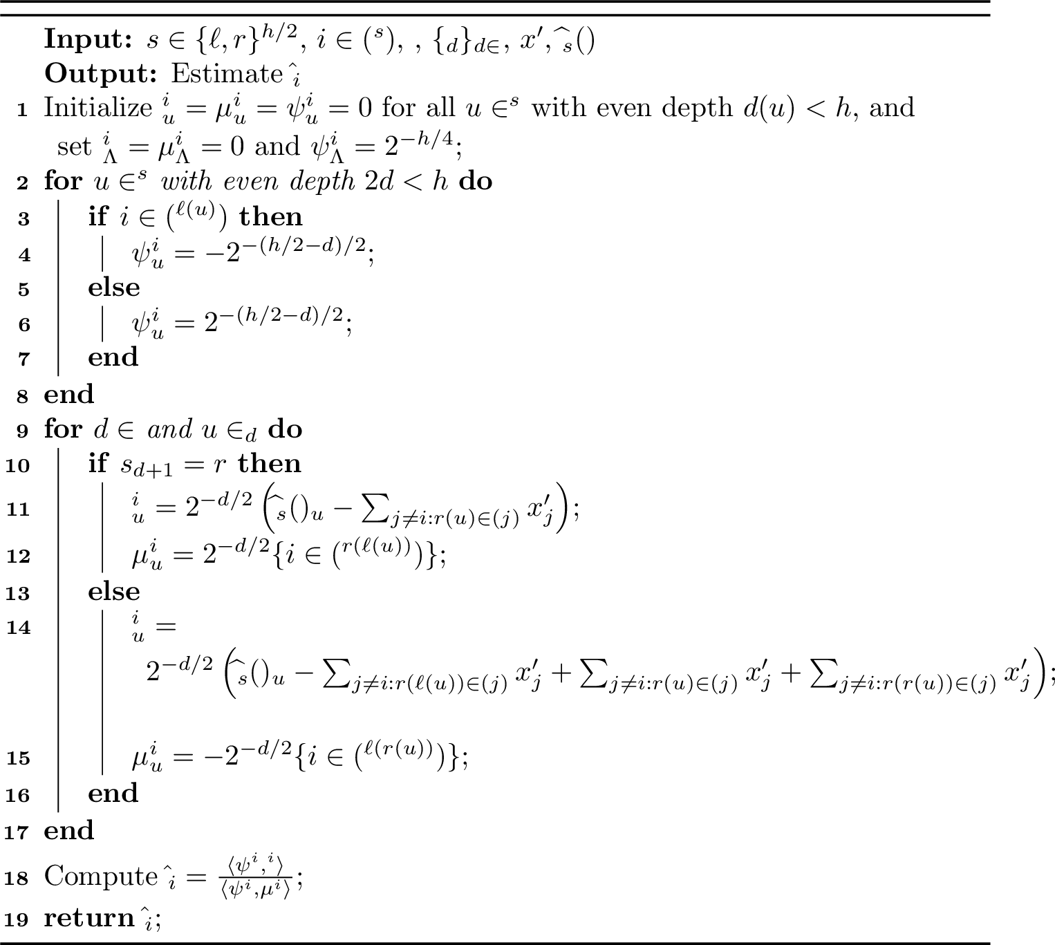
In essence, the adversary performs a privacy attack via linear measurements \(\psi^i\). The vectors \(\psi^i\) are inspired by the Haar wavelet basis and are defined independently of \(\mathbf{x}\). The key step is to show that the vector \(\mathbf{c}^i\) computed by the adversary can be decomposed as \[\mathbf{c}^i = \mathbf{x}_i \mu^i + \mathbf{r},\] where \(\mu^i\) is a deterministic vector depending only on \(i\), \(s\), \(\mathcal{J}\), \(\{\mathcal{J}_d\}_{d\in\mathcal{J}}\), and \(\mathbf{r}\) is a noise vector whose \(\ell_2\) norm is controlled by \(\sigma\). Given this decomposition, the adversary computes \[\hat{\mathbf{x}}_i = \frac{\langle \psi^i, \mathbf{c}^i \rangle}{\langle \psi^i, \mu^i \rangle} = \mathbf{x}_i + \frac{\langle \psi^i, \mathbf{r}\rangle}{\langle \psi^i, \mu^i \rangle},\] which is a private estimate of \(\mathbf{x}_i\) with additive noise \(\langle \psi^i, \mathbf{r}\rangle / \langle \psi^i, \mu^i\rangle\). We now establish the decomposition \(\mathbf{c}^i = \mathbf{x}_i\mu^i + \mathbf{r}\).
For each \(u \in \mathcal{V}(\mathcal{T})\), let \(\mathbf{a}_u = \sum_{i : u \in \mathcal{I}(i)} \mathbf{x}_i\) so that \(A\mathbf{x}= \sum_{u \in \mathcal{V}(\mathcal{T})} \mathbf{a}_u \chi^u\). For every \(d \in \mathcal{J}\) and every \(u \in \mathcal{J}_d\), if \(s_{d+1}=r\), the adversary subtracts \[\sum_{j \neq i : r(u) \in \mathcal{I}(j)} \mathbf{x}_j\] from \(\widehat{\mathbf{M}}_s(\mathbf{x})_u\) to obtain \[\begin{align} &\widehat{\mathbf{M}}_s(\mathbf{x})_u - \sum_{j \neq i : r(u) \in \mathcal{I}(j)} \mathbf{x}_j= \mathbf{q}_u + \mathbf{a}_{r(u)} - \sum_{j \neq i : r(u) \in \mathcal{I}(j)} \mathbf{x}_j = \mathbf{q}_u+ \mathbb{1}\{r(u) \in \mathcal{I}(i)\} \mathbf{x}_i, \end{align}\] where \(\mathbf{q}_u\) is defined as in 13 . We observe that for \(s_{d+1}=r\) we have that \(i\) is in either the subtree rooted at \(r(\ell(u))\) or \(r(r(u))\) and thus \(\mathbb{1}\{r(u) \in \mathcal{I}(i)\} =\mathbb{1}\{i \in \mathcal{L}(\mathcal{T}^{r(\ell(u))})\}\). The adversary has thus computed \[\mathbf{q}_u + \mathbb{1}\{i \in \mathcal{L}(\mathcal{T}^{r(\ell(u))})\}\mathbf{x}_i.\] Now multiply this by \(2^{-d/2}\) to obtain \[\mathbf{c}_u^i = 2^{-d/2}\left(\mathbf{q}_u + \mathbb{1}\{i \in \mathcal{L}(\mathcal{T}^{r(\ell(u))})\}\mathbf{x}_i\right).\] If instead \(s_{d+1}=\ell\), the adversary subtracts \[\sum_{j \neq i: r(\ell(u)) \in \mathcal{I}(j)} \mathbf{x}_j - \sum_{j \neq i: r(u) \in \mathcal{I}(j)} \mathbf{x}_j -\sum_{j \neq i: r(r(u)) \in \mathcal{I}(j)} \mathbf{x}_j\] from \(\widehat{\mathbf{M}}_s(\mathbf{x})_u\) to obtain \[\begin{align} &\widehat{\mathbf{M}}_s(\mathbf{x})_u - \left( \sum_{j \neq i: r(\ell(u)) \in \mathcal{I}(j)} \mathbf{x}_j - \sum_{j \neq i: r(u) \in \mathcal{I}(j)} \mathbf{x}_j -\sum_{j \neq i: r(r(u)) \in \mathcal{I}(j)} \mathbf{x}_j \right)=\\ &\mathbf{q}_u + \mathbf{a}_{r(\ell(u))} -\mathbf{a}_{r(u)} - \mathbf{a}_{r(r(u))} - \left( \sum_{j \neq i: r(\ell(u)) \in \mathcal{I}(j)} \mathbf{x}_j - \sum_{j \neq i: r(u) \in \mathcal{I}(j)} \mathbf{x}_j -\sum_{j \neq i: r(r(u)) \in \mathcal{I}(j)} \mathbf{x}_j \right) =\\ & \mathbf{q}_u + \left(\mathbb{1}\{r(\ell(u)) \in \mathcal{I}(i)\} - \mathbb{1}\{r(u) \in \mathcal{I}(i)\}- \mathbb{1}\{r(r(u)) \in \mathcal{I}(i)\} \right)\mathbf{x}_i, \end{align}\] where \(\mathbf{q}_u\) is defined in 14 . Since for \(s_{d+1}=\ell\) we have that \(i\) is either in the subtree rooted at \(\ell(\ell(u))\) or at \(\ell(r(u))\), we conclude by the definition of \(\mathcal{I}(i)\) that if \(i \in \mathcal{L}(\mathcal{T}^{\ell(\ell(u))})\), we have \[\begin{align} &\mathbb{1}\{r(\ell(u)) \in \mathcal{I}(i)\} - \mathbb{1}\{r(u) \in \mathcal{I}(i)\}- \mathbb{1}\{r(r(u)) \in \mathcal{I}(i)\} = 1-1-0 = 0. \end{align}\] and if \(i \in \mathcal{L}(\mathcal{T}^{\ell(r(u))})\) we have \[\begin{align} &\mathbb{1}\{r(\ell(u)) \in \mathcal{I}(i)\} - \mathbb{1}\{r(u) \in \mathcal{I}(i)\}- \mathbb{1}\{r(r(u)) \in \mathcal{I}(i)\} = 0-0-1 = -1. \end{align}\] The adversary has thus computed \[\mathbf{q}_u - \mathbb{1}\{i \in \mathcal{L}(\mathcal{T}^{\ell(r(u))})\}\mathbf{x}_i.\] Now multiply this by \(2^{-d/2}\) to obtain \[\mathbf{c}_u^i = 2^{-d/2}\left(\mathbf{q}_u - \mathbb{1}\{i \in \mathcal{L}(\mathcal{T}^{\ell(r(u))})\}\mathbf{x}_i \right).\]
Now define a vector \(\mathbf{r}\) with one coordinate \(\mathbf{r}_u\) for each \(u \in \mathcal{T}^s\) at an even depth less than \(h\) and an additional dummy coordinate \(\mathbf{r}_\Lambda = 0\). Define \(\mathbf{r}_u = 0\) for \(u \notin \cup_{d \in \mathcal{J}} \mathcal{J}_d\) and define \(\mathbf{r}_u = 2^{-d/2} \mathbf{q}_u\) otherwise. By the above arguments, \(\mathbf{c}^i = \mathbf{x}_i \mu^i + \mathbf{r}\), establishing the promised decomposition. For \(i \in \mathcal{L}(\mathcal{T}^s)\), the adversary computes the estimate \[\hat{\mathbf{x}}_i = \frac{\langle \psi^i, \mathbf{c}^i\rangle}{\langle \psi^i, \mu^i \rangle}=\frac{\langle \psi^i, \mathbf{r}+ \mathbf{x}_i \mu^i\rangle}{\langle \psi^i, \mu^i \rangle} = \mathbf{x}_i + \frac{\langle \psi^i, \mathbf{r}\rangle}{\langle \psi^i, \mu^i \rangle}.\]
Since \(\hat{\mathbf{x}}_i\) is a deterministic function of \(\widehat{\mathbf{M}}_s(\mathbf{x})\) and \(x'\), it is \((6\varepsilon, 3e\delta)\)-differentially private by the postprocessing property of differential privacy. Moreover, \(\hat{\mathbf{x}}_i\) is an estimate of the binary variable \(\mathbf{x}_i\) with additive noise \(\frac{\langle \psi^i, \mathbf{r}\rangle}{\langle \psi^i, \mu^i \rangle}\), which is independent of \(\mathbf{x}_i\). This is because \(\mathbf{r}\) only depends on \(s\), \(\mathcal{J}\), \(\{\mathcal{J}_d\}_{d\in \mathcal{J}}\), and the noise vectors \(\mathbf{z}^{(1)}, \mathbf{z}^{(2)}, \mathbf{z}^{(3)}\) (which are independent of \(\mathbf{x}\) because \(\mathbf{M}_o\) is oblivious). We observe that none of \(\psi^i\), \(\mu^i\), \(\mathbf{r}\) depend on \(x'\): \(\psi^i\) depends on \(i\) and \(s\), \(\mu^i\) depends on \(i, s, \mathcal{J}, \{\mathcal{J}_d\}_{d\in \mathcal{J}}\) and \(\mathbf{r}\) depends on \(s, \mathcal{J}, \{\mathcal{J}_d\}_{d \in \mathcal{J}}\) and the noise vectors \(\mathbf{z}^{(1)}, \mathbf{z}^{(2)}, \mathbf{z}^{(3)}\). Applying Lemma 1, we conclude that for fixed \(s, i, \mathcal{J}, \{\mathcal{J}_d\}_{d \in \mathcal{J}}\) as defined above
\[\begin{align} \frac{\mathbb{E}[\langle \psi^i,\mathbf{r}\rangle^2]}{\langle\psi^i, \mu^i \rangle^2} = \Omega( \min\{6^{-2} \varepsilon^{-2}, (3e)^{-2}\delta^{-2}\}). \end{align}\] Therefore, for fixed \(s, \mathcal{J}, \{\mathcal{J}_d\}_{d \in \mathcal{J}}\) \[\begin{align} \label{eq:connecting-inequality} \sum_{i \in \mathcal{L}(\mathcal{T}^s)}\mathbb{E}[\langle \psi^i,\mathbf{r}\rangle^2] = \Omega\left( \sum_{i \in \mathcal{L}(\mathcal{T}^s)}\langle\psi^i, \mu^i \rangle^2 \min\{6^{-2} \varepsilon^{-2}, (3e)^{-2}\delta^{-2}\}\right). \end{align}\tag{15}\]
We now want to upper bound \(\sum_{i \in \mathcal{L}(\mathcal{T}^s)}\mathbb{E}[\langle \psi^i,\mathbf{r}\rangle^2]\) and lower bound \(\sum_{i \in \mathcal{L}(\mathcal{T}^s)}\langle\psi^i, \mu^i \rangle^2\), which will give us a lower bound on \(\sigma\).
We start by upper bounding \(\sum_{i \in \mathcal{L}(\mathcal{T}^s)}\mathbb{E}[\langle \psi^i,\mathbf{r}\rangle^2]\). Observe that the \(\psi^i\) vectors are orthogonal and unit length.
Lemma 5. For \(i \in \mathcal{L}(\mathcal{T}^s)\) we have \(\|\psi^i\|^2_2 = 1\) and for \(i \neq j\) with \(i,j \in \mathcal{L}(\mathcal{T}^s)\), we have \(\langle \psi^i, \psi^j \rangle = 0\).
This lemma follows directly from the definition of \(\psi^i\) and the proof has been deferred to Appendix 6. It follows from orthogonality and unit length that \(\sum_{i\in \mathcal{L}(\mathcal{T}^s)} \mathbb{E}[\langle \psi^i ,\mathbf{r}\rangle^2] = \mathbb{E}[\sum_{i\in \mathcal{L}(\mathcal{T}^s)} \langle \psi^i ,\mathbf{r}\rangle^2] \leq \mathbb{E}[\|\mathbf{r}\|_2^2]\). Now recall that \(\sigma = \max_{d \in \mathcal{J}} \max_{u \in \mathcal{J}_d} \sigma_{u, \widetilde{s_{d+1}}}\). We observe that \[\begin{align} \label{eq:ub} \mathbb{E}[\|\mathbf{r}\|_2^2] &= \sum_{d \in \mathcal{J}} \sum_{u \in \mathcal{J}_d} \mathbb{E}[\mathbf{r}_u^2] \nonumber\\ &\leq \sum_{d \in \mathcal{J}} \sum_{u \in \mathcal{J}_d} 3 \cdot 2^{-d} \cdot \sigma^2_{u, \widetilde{s_{d+1}}} \nonumber\\ &\leq 3 \cdot \sum_{d \in \mathcal{J}} \sum_{u \in \mathcal{J}_d} 2^{-d} \cdot \sigma^2 \nonumber\\ &= 3 \cdot \sum_{d \in \mathcal{J}} |\mathcal{J}_d| 2^{-d} \cdot \sigma^2 \nonumber\\ &= (3/2) \cdot \sum_{d \in \mathcal{J}} 2^d\cdot 2^{-d} \cdot \sigma^2 \nonumber\\ &= (3/2) \cdot |\mathcal{J}| \cdot \sigma^2 \nonumber\\ &= (3/8) \cdot h \cdot \sigma^2. \end{align}\tag{16}\]
Next, we lower bound \(\sum_{i \in \mathcal{L}(\mathcal{T}^s)}\langle\psi^i, \mu^i \rangle^2\). Define for convenience the notation \(\mathop{\mathrm{Anc}}(i,d) \in \mathcal{T}\) as the ancestor of the \(i\)’th leaf at depth \(2d\). Let us next consider \[\begin{align} \label{eq:ipsq} &\sum_{i \in \mathcal{L}(\mathcal{T}^s)} \langle \psi^i, \mu^i \rangle^2 = \nonumber \\ &\sum_{i \in \mathcal{L}(\mathcal{T}^s)} \left(\sum_{d=0}^{h/2-1} \mu_{\mathop{\mathrm{Anc}}(i,d)}^i 2^{-(h/2-d)/2} (-1)^{\mathbb{1}\{i \in \mathcal{L}(\mathcal{T}^{\ell(\mathop{\mathrm{Anc}}(i,d))})\}}\right)^2. \end{align}\tag{17}\] Let \(u = \mathop{\mathrm{Anc}}(i,d)\) for short. Then \[\begin{align} &\mu^i_{u} (-1)^{\mathbb{1}\{i \in \mathcal{L}(\mathcal{T}^{\ell(u)})\}} =\\ &2^{-d/2} (-1)^{\mathbb{1}\{s_{d+1}=\ell\}} \mathbb{1}\{i \in \mathcal{L}(\mathcal{T}^{s_{d+1}(\widetilde{s_{d+1}}(u))})\}(-1)^{\mathbb{1}\{i \in \mathcal{L}(\mathcal{T}^{\ell(u)})\}}. \end{align}\] Now consider first the case \(s_{d+1}=\ell\). Then \(\mathbb{1}\{i \in \mathcal{L}(\mathcal{T}^{s_{d+1}(\widetilde{s_{d+1}}(u))})\} = 0\) if \(i \in \mathcal{L}(\mathcal{T}^{\ell(u)})\). If instead \(i \in \mathcal{L}(\mathcal{T}^{r(u)})\), we get \[(-1)^{\mathbb{1}\{s_{d+1}=\ell\}} (-1)^{\mathbb{1}\{i \in \mathcal{L}(\mathcal{T}^{\ell(u)})\}}= -1 \cdot 1 = -1.\] Similarly, if \(s_{d+1}=r\), then we need only consider \(i \in \mathcal{L}(\mathcal{T}^{\ell(u)})\). Here we have \[(-1)^{\mathbb{1}\{s_{d+1}=\ell\}} (-1)^{\mathbb{1}\{i \in \mathcal{L}(\mathcal{T}^{\ell(u)})\}}= 1 \cdot (-1) = -1.\] Thus in all circumstances, we may simplify \[\begin{align} &\mu^i_{u} (-1)^{\mathbb{1}\{i \in \mathcal{L}(\mathcal{T}^{\ell(u)})\}} = -2^{-d/2} \mathbb{1}\{i \in \mathcal{L}(\mathcal{T}^{s_{d+1}(\widetilde{s_{d+1}}(u))})\}. \end{align}\] Inserting this in 17 , we see that \[\begin{align} &\sum_{i \in \mathcal{L}(\mathcal{T}^s)} \langle \psi^i, \mu^i \rangle^2 = \\ &\sum_{i \in \mathcal{L}(\mathcal{T}^s)} \left(\sum_{d=0}^{h/2-1} -2^{-h/4}\mathbb{1}\{i \in \mathcal{L}(\mathcal{T}^{s_{d+1}(\widetilde{s_{d+1}}(\mathop{\mathrm{Anc}}(i,d)))})\} \right)^2 =\\ &2^{-h/2} \sum_{i \in \mathcal{L}(\mathcal{T}^s)} \left(\sum_{d=0}^{h/2-1} \mathbb{1}\{i \in \mathcal{L}(\mathcal{T}^{s_{d+1}(\widetilde{s_{d+1}}(\mathop{\mathrm{Anc}}(i,d)))})\} \right)^2 = \\ &2^{-h/2} \sum_{i \in \mathcal{L}(\mathcal{T}^s)} \sum_{d=0}^{h/2-1} \sum_{d'=0}^{h/2-1} \mathbb{1}\{i \in \mathcal{L}(\mathcal{T}^{s_{d+1}(\widetilde{s_{d+1}}(\mathop{\mathrm{Anc}}(i,d)))})\}\mathbb{1}\{i \in \mathcal{L}(\mathcal{T}^{s_{d'+1}(\widetilde{s_{d'+1}}(\mathop{\mathrm{Anc}}(i,d')))})\} = \\ &2^{-h/2} \sum_{d=0}^{h/2-1} \sum_{d'=0}^{h/2-1} \sum_{u \in \mathcal{J}_d} \sum_{v \in \mathcal{J}_{d'}} \sum_{i \in \mathcal{L}(\mathcal{T}^s)}\mathbb{1}\{i \in \mathcal{L}(\mathcal{T}^{s_{d+1}(\widetilde{s_{d+1}}(u))})\}\mathbb{1}\{i \in \mathcal{L}(\mathcal{T}^{s_{d'+1}(\widetilde{s_{d'+1}}(v))})\}. \end{align}\] Now define vectors \(\phi^u\) for each \(u \in \cup_{d \in \mathcal{J}} \mathcal{J}_d\). If \(u\) is in depth \(2d\), we let \(\phi^u\) be the indicator vector with one coordinate for each \(i \in \mathcal{L}(\mathcal{T}^s)\) taking the value \(\mathbb{1}\{i \in \mathcal{L}(\mathcal{T}^{s_{d+1}(\widetilde{s_{d+1}}(u))})\}\). Then by the above we have \[\begin{align} &\sum_{i \in \mathcal{L}(\mathcal{T}^s)} \langle \psi^i, \mu^i \rangle^2 = 2^{-h/2} \left\|\sum_{u \in \cup_{d \in \mathcal{J}} \mathcal{J}_d} \phi^u \right\|^2_2. \end{align}\] Applying Cauchy-Schwartz, we first see that \[\begin{align} \label{eq:step1} 2^{-h/2} \left\|\sum_{u \in \cup_{d \in \mathcal{J}} \mathcal{J}_d} \phi^u \right\|^2_2 \geq &2^{-h/2} \left\|\sum_{u \in \cup_{d \in \mathcal{J}} \mathcal{J}_d} \phi^u \right\|^2_1 \cdot |\mathcal{L}(\mathcal{T}^s)|^{-1}. \end{align}\tag{18}\] Now using that the vectors \(\phi^u\) are indicator vectors we have that 18 equals \[\begin{align} &2^{-h} \left(\sum_{u \in \cup_{d \in \mathcal{J}} \mathcal{J}_d} \|\phi^u\|_1 \right)^2 = 2^{-h} \left(\sum_{d \in \mathcal{J}} \sum_{u \in \mathcal{J}_d} \|\phi^u\|_1 \right)^2 = 2^{-h} \left(\sum_{d \in \mathcal{J}} \sum_{u \in \mathcal{J}_d} 2^{h/2-d-1} \right)^2 =\\ &2^{-h} \left(\sum_{d \in \mathcal{J}} 2^{d-1} 2^{h/2-d-1} \right)^2 = 2^{-h} \left(h \cdot 2^{h/2-4} \right)^2 = 2^{-8} h^2. \end{align}\] Therefore, \[\begin{align} \sum_{i \in \mathcal{L}(\mathcal{T}^s)} \langle \psi^i, \mu^i \rangle^2\geq 2^{-8} h^2. \label{eq:lb} \end{align}\tag{19}\]
Using the upper bound of \(\mathbb{E}[\|\mathbf{r}\|^2]\) 16 and the lower bound of \(\sum_{i \in \mathcal{L}(\mathcal{T}^s)}\langle \psi^i, \mu^i\rangle^2\) 19 in inequality 15 , it follows that \[\frac{3 \cdot h\cdot \sigma^2}{8} \geq \Omega(h^2 \cdot 2^{-8} \min\{6^{-2} \varepsilon^{-2}, (3e)^{-2}\delta^{-2}\}).\] This gives a lower bound of \[\sigma^2 = \Omega(h \min\{\varepsilon^{-2},\delta^{-2}\}) \Rightarrow \sigma = \Omega(\sqrt{h} \min\{\varepsilon^{-1},\delta^{-1}\}).\] Inserting this in 10 and 12 we conclude \[\max_{x \in \{0,1\}^n }\mathbb{E}[\|\mathbf{M}(x)-Ax\|_\infty] \geq \mathbb{E}[\|\mathbf{z}\|_\infty] = \Omega\left(\frac{h^{3/2}}{\max\{\varepsilon,\delta\}} \right) = \Omega\left(\frac{\log^{3/2} n}{\max\{\varepsilon,\delta\}} \right).\] This completes the proof of Theorem 1.
5 Median-of-Three Trick↩︎
Here we show how to derive Corollary 1 from the work of [29]. For the proof, we use the following auxiliary result by Larsen, Pagh and Tetek:
Lemma 6 ([29]). Let \(f: \mathbb{R}^+ \to \mathbb{R}^+\) be a non-increasing function and let \(t\) be a positive integer. Then \[\int_{x=0}^\infty f(x^{1/t})^t dx \leq \left( \int_{x=0}^\infty f(x) dx\right)^t.\]
Proof of Corollary 1. We have \[\begin{align} \mathbb{E}[\mathop{\mathrm{median}}\{\mathbf{Z}_1,\mathbf{Z}_2,\mathbf{Z}_3\}^2] &\leq \mathbb{E}[\min\{|\mathbf{Z}_1|,|\mathbf{Z}_2|\}^2] + \mathbb{E}[\min\{|\mathbf{Z}_1|,|\mathbf{Z}_3|\}^2] +\mathbb{E}[\min\{|\mathbf{Z}_2|,|\mathbf{Z}_3|\}^2] \\ &= 3 \cdot \mathbb{E}[\min\{\mathbf{Z}_1^2,\mathbf{Z}_2^2\}]. \end{align}\] Let \(p_x = \Pr[|\mathbf{Z}_1| > x]\) and recall the layer-cake formula \(\mathbb{E}[|\mathbf{Z}_1|] = \int_{x=0}^\infty p_x dx\). By independence of \(\mathbf{Z}_1,\mathbf{Z}_2\), we get \[\begin{align} \mathbb{E}[\min\{\mathbf{Z}_1^2,\mathbf{Z}_2^2\}] &\leq \int_{x=0}^\infty \Pr[\mathbf{Z}_1^2 > x \wedge \mathbf{Z}_2^2 > x ] dx \\ &= \int_{x=0}^\infty \Pr[\mathbf{Z}_1^2 > x ]^2 dx \\ &= \int_{x=0}^\infty \Pr[|\mathbf{Z}_1| > \sqrt{x} ]^2 dx \end{align}\] Letting \(f(x) = \Pr[|\mathbf{Z}_1| > x ]\), we get from Lemma 6 that \[\begin{align} \mathbb{E}[\mathop{\mathrm{median}}\{\mathbf{Z}_1,\mathbf{Z}_2,\mathbf{Z}_3\}^2] &\leq 3\cdot \left( \int_{x=0}^\infty \Pr[|\mathbf{Z}_1] > x] dx \right)^2 \\ &= 3 \cdot \mathbb{E}[|\mathbf{Z}_1|]^2. \end{align}\] ◻
6 Properties of Attack Vectors↩︎
Here we prove Lemma 5, stating that the \(\psi^i\) vectors are orthogonal and unit length.
Proof of Lemma 5. Let \(i \neq j\) with \(i,j \in \mathcal{L}(\mathcal{T}^s)\). Then \[\begin{align} \langle \psi^i, \psi^j \rangle &= 2^{-h/2} + \sum_{u : i,j \in \mathcal{L}(\mathcal{T}^u)} 2^{-(h/2-d)} (-1)^{\mathbb{1}\{i \in \mathcal{L}(\mathcal{T}^{\ell(u)})\} + \mathbb{1}\{j \in \mathcal{L}(\mathcal{T}^{\ell(u)})\}} \end{align}\] If \(u\) denotes the lowest common ancestor of the \(i\)’th and \(j\)’th leaf, and \(u\) is at depth \(2d\), then \(u\) contributes \(-2^{-(h/2-d)}\) to the inner product, the \(k\)’th ancestor of \(u\) contributes \(2^{-k} 2^{-(h/2-d)}\), and all other nodes contribute \(0\). Finally, the dummy coordinate contributes \(2^{-h/2}\). Hence the inner product precisely equals \[-2^{-(h/2-d)} + 2^{-h/2} + \sum_{k=1}^d 2^{-k} 2^{-(h/2-d)} = -2^{-(h/2-d)} + 2^{-h/2} + 2^{-(h/2-d)} - 2^{-h/2} = 0.\] Thus the \(\psi^i\) vectors are orthogonal. We also have \[\begin{align} \|\psi^i\|_2^2 &= 2^{-h/2} + \sum_{d=0}^{h/2-1} 2^{-(h/2-d)} = 1. \end{align}\] ◻