Overlapping Domain Decomposition for Meshless Finite Difference Methods
July 01, 2026
1 Introduction↩︎
Schwarz’s domain decomposition going back to [1] is used in modern mesh-based discretization methods either as a stand-alone iterative method for solving linear systems, or as a preconditioner. In particular, it is applied to saddle point problems, such as the Stokes or Navier-Stokes equations, for which no classical iterative methods can be used due to the matrix structure [2], [3].
Furthermore, numerous papers on finite elements, for example [2], [4], [5], have discussed the application of the additive Schwarz method as a smoother in multigrid methods, with a focus on decomposing into very small subdomains (batch- or cell-based). These methods originate from the work of Vanka [6], which employed a symmetric coupled Gauss-Seidel smoother that can be identified as an algebraic Schwarz method.
In this paper we explore the application of the additive Schwarz method to linear systems arising from a meshless finite difference method on irregular nodes. The main question is how to design subdomains without the help of a mesh, and we demonstrate that a crucial parameter is the amount of the overlap between different subdomains. In mesh-based methods it is common [7] to use subdomains that build a disjoint partition of the full computation domain. However, our experiments show that this is undesirable for the meshless methods.
The second question we address is the influence of the choice of the partition of unity (PoU) used to combine subsolutions when subdomains overlap. It turns out that both versions of the algebraic additive Schwarz method introduced in [8], the restricted additive Schwarz method (RAS) and the additive Schwarz method with harmonic extension (ASH) perform well in the meshless setting if PoU is continuous, but ASH typically outperforms RAS with the simpler discontinuous PoU.
In our numerical experiments we discretize a Poisson problem in 1D and 2D and a Stokes problem in 2D by using the radial basis function finite difference (RBF-FD) method with polyharmonic RBF and a polynomial extension, see for example [9].
The paper is organized as follows. After a brief Section 2 that introduces the two versions of the iterative Schwarz methods RAS and ASH studied in this paper in the meshless context, we present in Section 3 our numerical investigation of their performance in conjunction with two types of PoU for three examples of boundary value problems. Section 4 provides a conclusion.
2 Schwarz methods↩︎
Various types of iterative Schwarz methods are summarized in Fig. 1. It starts with a global continuous problem on the top, for example the Poisson equation with Dirichlet boundary conditions \[\begin{align} \left.\begin{cases} -\Delta u=f & \text{in }\Omega\\ \phantom{-\Delta}u = g & \text{on } \Gamma=\partial\Omega \end{cases}\right\}. \end{align}\] The two main branches in Fig. 1 are distinguished by whether decomposition or discretization is applied first.
The general idea behind every Schwarz method is as follows: If the problem is too big or the geometry is too complex, then several subproblems corresponding to different subdomains of \(\Omega\) are solved, and these solutions are combined into an approximation of the global problem. By iterating this process the convergence of the global approximation is achieved. For the sake of simplicity of the exposition we only formulate the subdivision into two subproblems on subdomains \(\Omega_1\) and \(\Omega_2\), with \(\bar\Omega=\bar\Omega_1\cup\bar\Omega_2\). Furthermore, only the additive version of the Schwarz method without any optimization, such as the optimized RAS in [10], is considered.
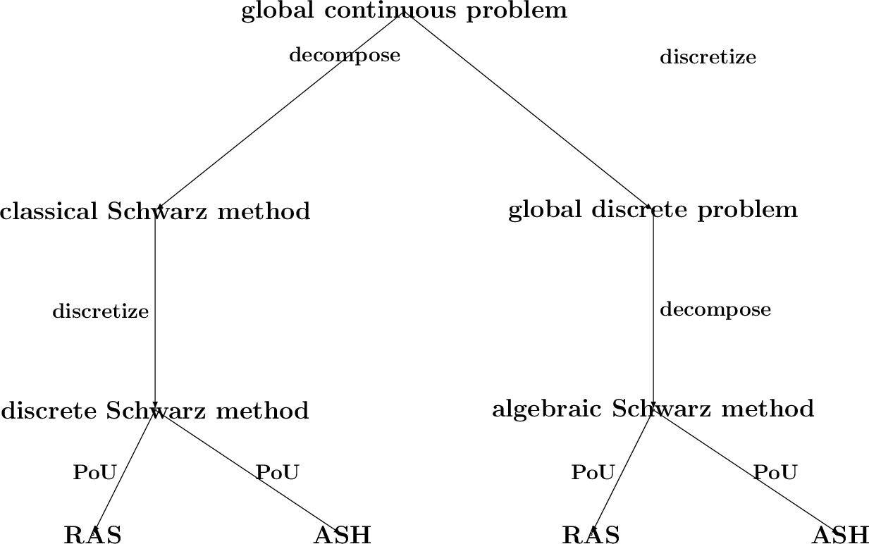
By applying the decomposition to the global problem, the decomposed continuous problem can be formulated with a starting solution \(u^0\) and \(n\ge0\) \[\begin{align} \left.\begin{cases} -\Delta v^{n+1}=f^{(1)} & \text{in }\Omega_1\\ \phantom{-\Delta}v^{n+1} = g^{(1)} & \text{on } \Gamma_1=\partial\Omega_1 \end{cases}\right\}\quad\wedge\quad \left.\begin{cases} -\Delta w^{n+1}=f^{(2)} & \text{in }\Omega_2\\ \phantom{-\Delta}w^{n+1} = g^{(2)} & \text{on } \Gamma_2=\partial\Omega_2 \end{cases}\right\} \end{align}\] where \(v^{n+1}\) and \(w^{n+1}\) are the solutions of each subproblem, whereas \(f^{(i)}=f|_{\Omega_i}\), \(g^{(i)}=u_n|_{\Gamma_i}\), \(i=1,2\). The new global solution \(u^{n+1}\) is computed using prolongation operators \(P_1\) and \(P_2\) that extend \(v^{n+1}\) and \(w^{n+1}\) to \(\Omega\), and a combining operator \(C\) resulting in \(u^{n+1} = C\left(P_1 v^{n+1}, P_2 w^{n+1}\right).\) This iterative algorithm is called the classical Schwarz method in this work. After some numerical methods are applied to solve the continuous subproblems and operators \(P_i\) and \(C\) are also implemented numerically, a discrete Schwarz method is defined that produces a discrete approximation \(u^{n+1}_h\) of \(u^{n+1}\).
The second branch of the family tree starts with the discretization instead of the decomposition so that a global discrete problem \[\begin{align} \left.\begin{cases} A_h u_h = f_h & \text{in }\Omega_h\\ \phantom{A_h}u_h = g_h & \text{on } \Gamma_h \end{cases}\right\} \end{align}\] is set up. Here, the subscript \(h\) symbolizes the discrete version of each function as a vector, \(A_h\) stands for a matrix that represents the discrete Poisson operator, and \(\Omega_h\) and \(\Gamma_h\) are the discretized domain and its boundary, given by a grid or mesh, or just a node set in the case of meshless methods. Similar to the classical Schwarz method, the decomposition process can be applied to the discrete problem by selecting matrix and vector entries corresponding to the indices of each discrete subdomain \(\Omega_{h,i}\subset\Omega_h\). In this paper we consider only the trivial prolongation operators, whereby continuous solutions are extended by zero outside of \(\Omega_i\) and the discrete vectors are filled with zeros to match the size of the global vectors.
One possible realization of combining multiple local solutions into a global one is to use a partition of unity. For that we choose PoU functions \(\varphi_i\) that satisfy \(\Omega_i\subset\mathop{\mathrm{supp}}\varphi_i\) and sum up to one globally, that is, in the case of two subdomains \(\varphi_1+\varphi_2 \equiv 1\) in \(\Omega\), leading to the combining operator \(C\big(v, w\big)={\varphi_1}v + {\varphi_2}w\). Thus, the global solution is obtained in the continuous case as \[u^{n+1}={\varphi_1}P_1 v^{n+1} + {\varphi_2}P_2w^{n+1}=u^{n}+{\varphi_1}P_1 v_{\delta}^{n+1} + {\varphi_2}P_2w_{\delta}^{n+1},\] where the second version uses the residuals \(v_{\delta}^{n+1}=v^{n+1}-u^{n}\) and \(w_{\delta}^{n+1}=w^{n+1}-u^{n}\).
The discrete algebraic Schwarz method is called restricted additive Schwarz (RAS) preconditioner in [8]. In the same paper Cai and Sarkis also introduced the additive Schwarz method with harmonic extension (ASH) as a second way to include the PoU by applying it to the right hand sides of the subproblems before solving the linear systems. We formulate both RAS and ASH in the residual form: with a global initial solution vector \(u_h^0\) and \(n\ge0\),
RAS: apply the PoU after solving each subproblem.
Solve subsystems:
Obtain a global solution from the subsolutions \(v_{\delta, h}^{n+1},w_{\delta, h}^{n+1}\): \[u_h^{n+1} = u_h^n + {\varphi_{h,1}}P_{h,1} v_{\delta, h}^{n+1} + {\varphi_{h,2}}P_{h,2} w_{\delta, h}^{n+1}.\]ASH: Apply the PoU before solving each subproblem:
Solve subsystems:
Obtain a global solution from the subsolutions \(v_{\delta, h}^{n+1},w_{\delta, h}^{n+1}\): \[u_h^{n+1} = u_h^n + P_{h,1} v_{\delta,h}^{n+1} + P_{h,2} w_{\delta,h}^{n+1}.\]
The iterations are repeated until the root mean square residual \(P_{h,1} v_{\delta,h}^{n+1} + P_{h,2} w_{\delta,h}^{n+1}\) reduces below a given tolerance \(\varepsilon>0\). We used \(\varepsilon=10^{-7}\) in all numerical experiments.
3 Numerical results↩︎
In the numerical experiments we will use two types of PoU:
dPoU: A discontinuous PoU depending on how many subdomain include a point \(x\): \[\varphi_i(x) = \begin{cases} \big(\#\{k=1,\ldots,N_{DEC}:x\in\Omega_k\}\big)^{-1}, & x\in\Omega_i,\\ 0, & \text{otherwise}, \end{cases}\] where \(N_{DEC}\) is the number of subdomains. The property \(\sum_i \varphi_i = 1\) is directly fulfilled.
cPoU: A continuous PoU as a bump function depending on the the choice of centers \(z_i\in\Omega_i\) and the maximum distance \(r_i := \sup\{\|x-z_i\|_2:x\in\Omega_i\}\) of the subdomain \(\Omega_i\): \[\tilde{\varphi}_i(x) =\begin{cases} \exp\Big(-\frac{r_i^2}{r_i^2 - \|x-z_i\|_2^2}\Big), & x\in\Omega_i,\\ 0, & \text{otherwise}, \end{cases}\] with \(\varphi_i=\tilde{\varphi}_i/\sum_k \tilde{\varphi}_k\).
Each differential operator is discretized using the RBF-FD method with the PHS kernel of the form \(r^3\) and a polynomial extension of order 3 for the first derivatives and order 4 for the second derivatives, ensuring the convergence order of approximately 2, as discussed in [11] for the Stokes case. The sets of influence consist of the same number of nearest neighbors of a given node, in particular 10 for the Poisson equation in 1D, and 25 for the 2D Poisson case. In the case of the Stokes equations, the numbers are 20 for the gradient and divergence, and 25 for the Laplacian.
Discretization nodes are obtained from the quasi-random Halton sequence.
All computations were performed on a machine with an Intel Xeon E5-2640 v3 CPU (2.60 GHz) using MATLAB R2024b and basic MATLAB functions of mFDlab [12] for RBF-FD.
We use direct solvers to obtain the subsolutions because they are relatively small and we also want to exploit the important advantage of the algebraic Schwarz method that the submatrices remain unchanged throughout the iteration process. Therefore, we
compute LU decompositions of the matrices \(A_h^{(i)}\) only once before the iteration starts by MATLAB’s lu command, and solve the linear systems within the iteration loop by forward and backward substitution
using MATLAB’s backslash operator.
3.1 Poisson 1D↩︎
In the first test, we consider a one-dimensional Poisson problem, similar to the example provided in [13], with the solution \(u(x) = 0.5\left(x-x^2\right)\) on the unit interval \([0,1]\). The domain is decomposed into two overlapping subdomains \(\Omega = \Omega_1\cup\Omega_2\) where \(\Omega_1 = (0,\frac{2}{3})\) and \(\Omega_2 = (\frac{1}{3},1)\).
Fig. 2 (a)–(b) visualizes the iterative process of the global solution for the RAS method. It can be seen that the two different PoUs result in subsolutions of different character. On the one hand, if a discontinuous PoU is applied, a discontinuous global solution is obtained. This is natural since a discontinuous function is applied to globalizing continuous subsolutions. On the other hand, the application of the continuous PoU delivers a continuous global solution. This phenomenon disappears for ASH, where the PoU is applied before solving the subproblems. Moreover, as can be seen Fig. 2 (c)–(d), there is no significant difference between the solutions obtained with dPoU and cPoU.

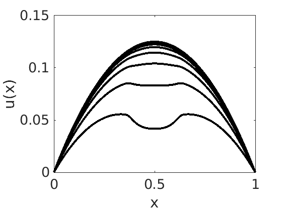
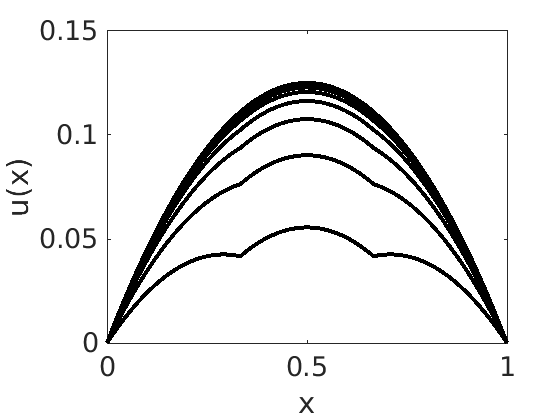

Figure 2: Iterative solution process of algebraic Schwarz method in different combinations of RAS or ASH versions and discontinuous or continuous PoU. a — RAS-dPoU, b — RAS-cPoU, c — ASH-dPoU, d — ASH-cPoU
Discontinuous subsolutions in the RAS-dPoU version have a significant drawback compared with the ASH-style version. First, a discontinuous approximation is clearly undesirable for a smooth solution of the continuous problem. Moreover, the residuum of the discrete Poisson operator is much greater in this case because the discrete Poisson operator is applied to a discontinuous solution. This leads to a higher tolerance for the termination condition, and, in combination with a high condition number of the global matrix, to RAS-dPoU not converging in terms of the global residual error for finer discretizations. We will demonstrate that even for smaller systems with lower condition numbers, RAS-dPoU requires more iterations than ASH-dPoU to reach a given tolerance.
To compare the performance of the methods quantitatively, and investigate the dependence on the amount of the overlap, we set up the following experiments, both in 1D and 2D. The discretized domain \(\Omega_h\) with
\(N_{max}\) nodes is decomposed into \(N_{DEC}\) nearly disjoint subdomains \(\Omega_{h,i}\) of approximately the same size \(N_{dis}\) with the help of MATLAB’s command kmeans that also returns the centroids of the subdomains. Each subdomain is then extended to achieve a desired number \(N\le N_{max}\) of
nodes, for \(N\in[N_{min},2N_{min},3N_{min},\dots]\) by including additional nodes within an increasing distance from the centroid until a given number \(N\) of nodes is reached. Here, \(N_{min}\ge N_{dis}\) is the minimum number of nodes required for the Schwarz method to deliver stable solutions, determined experimentally. We refer to Figures 4 and 6 for the illustrations in the 2D case. With this design of the experiments we ensure that the number of subdomains is fixed, which reduces the influence of parallel computation when we compare the influence of
the more or less significant overlap. To measure the amount of the overlap we compute the overlap ratio \[\rho(N) = \frac{N-N_{dis}}{N_{max}-N_{dis}},\] where \(N_{dis}\le N\le
N_{max}\) so that \(\rho\in[0,1]\). Thus, \(\rho=0\) stands for the disjoint decomposition and \(\rho=1\) for \(\Omega_i=\Omega\) for all \(i\in\{1,\dots,N_{DEC}\}\). This overlap ratio must be interpreted as a global parameter, and it can only provide information about the relative (local) overlap to a
certain extent.
In Fig. 3 and related figures below, we plot the number of iterations \(N_{iter}\) needed for the algebraic Schwarz method in RAS- and ASH-style with both discontinuous and
continuous PoU to converge. In addition, in order to demonstrate how the overlap ratio influences the overall computation cost, we plot the total computation time in seconds for the RAS method. Clearly, this timing depends on software and hardware. In our
tests the for-loops were implemented using MATLAB’s parfor command, with 16 parallel workers on our machine.
We observe from the results in Fig. 3 that the overall best configurations in 1D appear to be either RAS with continuous PoU or ASH with discontinuous PoU. In both cases the highest possible overlap is optimal, presumably due to the small bandwidth of the system matrix in 1D.
A relatively weak performance of RAS with discontinuous PoU is in a good agreement with the previous observations that discontinuous solutions produce higher residual errors, especially at the beginning of the iteration process.
It is surprising that the maximum overlap is optimal, even though in this case there is no decomposition as all subdomains coincide with \(\Omega\), and we in fact just repeat the same computation \(N_{DEC}\) times. However, as we will see, this does not anymore happen in 2D. A plausible explanation of this phenomenon is that the RBF-FD system matrices for the 1D Poisson equation are sparse and banded with a low bandwidth. Therefore, the direct method we use to solve the linear systems does not suffer from fill-in and requires just \(\mathcal{O}(N)\) operations, whereas no iterations are needed when the global system is solved, with its numerically zero residual.
3.2 Poisson 2D↩︎
The test problem for this section is the Poisson equation in \([0,1]^2\) with Dirichlet boundary conditions and solution \(u(x,y) = \sin(\pi x)\cos(\pi y)\). The setup of the experiments is the same as before. However, in contrast to 1D, where we used \(N_{min} = N_{dis}\), now \(N_{min}\) is greater than \(N_{dis}\) because otherwise the iterations do not converge, such that some minimum overlap seems to be required for mere stability. We illustrate in Fig. 4 typical choice of subdomains for in this case. We see that the overlap is almost negligible for \(N=N_{min}\), but already significant for \(N=2N_{min}\). Comparison of the number of iterations for RAS and ASH with dPoU and cPoU, as well as timing is provided in Fig. 5


Figure 3: Poisson 1D: Comparison of the number of iterations to convergence. (a)–(b): \(N_{max}=10^3\), \(N_{DEC} = 10\), \(N_{min}=100\); (c)–(d): \(N_{max}=10^4\), \(N_{DEC} = 20\), \(N_{min}=500\); (e)–(f): \(N_{max}=10^5\), \(N_{DEC} = 10\), \(N_{min}=10^4\).. a — discontinuous PoU, b — continuous PoU, c — discontinuous PoU, d — continuous PoU, e — discontinuous PoU, f — continuous PoU
In contrast to 1D, ASH now achieves smaller iteration numbers than RAS in almost all cases, even for the continuous PoU. For example, in the settings of Fig. 5 (e) and (f) for \(N=2N_{min}\), we have \(N_{iter}(RAS)=218\) versus \(N_{iter}(ASH)=161\), and \(N_{iter}(RAS)=152\) versus \(N_{iter}(ASH)=130\), respectively. Moreover, there is a striking change in how the computation time depends on the amount of overlap. After an initial step drop between until \(N\approx 2N_{min}\) or \(\rho\approx 0.05\), the time starts stabilizing for larger \(N\), and then grows, which is more pronounced for larger sizes of the global linear system. Clearly, this can be attributed to the higher bandwidth of the submatrices in two dimensions, and fill-in appearing in the cause of LU-decomposition of the submatrices.
In order to investigate the cost of the method more closely, we have estimated the numerical rate of the growth of the computation time as function of the size \(N\) of the submatrices. It turns out that the cost of computing the LU-decomposition of a single matrix \(A_h^{(i)}\) grows approximately at the rate \(\mathcal{O}(N^{1.8})\), while the cost of solving the system at each iteration is about \(\mathcal{O}(N^{1.4})\). This makes a big difference to the 1D case where both rates are \(\mathcal{O}(N)\) due to the absence of the fill-in, which explains the observed behavior.


Figure 5: Poisson 2D: Comparison of the number of iterations. (a)–(b): \(N_{max}=4225\), \(N_{DEC} = 25\), \(N_{min}=217\), \(N_{dis}=169\); (c)–(d): \(N_{max}=16641\), \(N_{DEC} = 25\), \(N_{min}=765\), \(N_{dis}=666\); (e)–(f): \(N_{max}=66049\), \(N_{DEC} = 25\), \(N_{min}=2866\), \(N_{dis}=2642\).. a — discontinuous PoU, b — continuous PoU, c — discontinuous PoU, d — continuous PoU, e — discontinuous PoU, f — continuous PoU
3.3 Stokes 2D↩︎
Finally, we consider the incompressible Stokes equations in \(\bar\Omega=[0,1]^2\) in the velocity-pressure formulation, \(\Delta \boldsymbol{u} + \nabla p = \boldsymbol{f}\) with \(\nabla\cdot \boldsymbol{u} = 0\) in \(\Omega\), and boundary conditions \(\boldsymbol{u} = \boldsymbol{g}\) on \(\partial\Omega\). The data \(\boldsymbol{f}\) and \(\boldsymbol{g}\) are chosen such that the velocity \(\boldsymbol{u}\) and the pressure \(p\) are defined as \(\boldsymbol{u}(x,y) = (\sin(\pi x)\cos(\pi y), -\sin(\pi y)\cos(\pi x))^T\) and \(p(x,y) = \sin(\pi x)\cos(\pi y)\) that defines an enclosed flow. Velocity \(\boldsymbol{u}\) and pressure \(p\) are discretized on two different sets of Halton nodes \(\Omega_{h,\boldsymbol{u}}\subset\bar\Omega\), and \(\Omega_{h,p}\subset \Omega_{h,\boldsymbol{u}}\cap \Omega\) chosen such that the stability condition established in Westermann et al. [11] is satisfied. In order to apply Schwarz’s method we need to decompose both \(\Omega_{h,\boldsymbol{u}}\) and \(\Omega_{h,p}\). In order to achieve stability we ensure that each subdomain is finer discretized for the velocity than for the pressure, and discrete subsets of nodes for both velocity and pressure exhibit a sufficient overlap. As before, we determine experimentally the minimum size of the subdomains that ensures convergence of the Schwarz iteration. The corresponding minimum number \(N_{min}^{\boldsymbol{u}}\) of velocity nodes in the subdomains is reported below as reference, whereas we keep the quotient between the number of pressure and velocity nodes at approximately \(1/4\) as suggested in [11].
Fig. 6 exemplifies the decomposition obtained for \(N^{\boldsymbol{u}}=2N_{min}^{\boldsymbol{u}}\) velocity nodes in the subdomains, with a near-optimal overlap in our tests, while Fig. 7 provides a comparison of the number of iterations and timing for RAS and ASH with dPoU and cPoU. The plots are only shown for \(\rho\in[0,0.5]\) as larger overlaps are of no interest due to a high computational cost.
We observe that ASH is preferred over RAS, however with only a small difference. The timing grows faster than in the case of Poisson 2D after passing the minimum at \(2N_{min}^{\boldsymbol{u}}\), which correlates with the higher cost of the solution by the direct method, with the rate \(\mathcal{O}(N^{2.8})\) for an LU-decomposition, and \(\mathcal{O}(N^{2})\) for solving the system at each iteration. This is due to the complex saddle-point structure of the Stokes equations, which has a higher bandwidth and is more susceptible to fill-in effects.


Figure 7: Stokes 2D: Comparison of the number of iterations. (a)–(b): \(N_{max}^{\boldsymbol{u}}=4225\), \(N_{DEC} = 25\), \(N_{min}^{\boldsymbol{u}}=290\), \(N_{dis}^{\boldsymbol{u}}=169\); (c)–(d): \(N_{max}^{\boldsymbol{u}}=4225\), \(N_{DEC} = 50\), \(N_{min}^{\boldsymbol{u}}=172\), \(N_{dis}^{\boldsymbol{u}}=85\); (e)–(f): \(N_{max}^{\boldsymbol{u}}=16641\), \(N_{DEC} = 25\), \(N_{min}^{\boldsymbol{u}}=926\), \(N_{dis}^{\boldsymbol{u}}=666\).. a — discontinuous PoU, b — continuous PoU, c — discontinuous PoU, d — continuous PoU, e — discontinuous PoU, f — continuous PoU
4 sec:Conclusion↩︎
In this paper, we studied the numerical behavior of the additive algebraic Schwarz method applied to boundary value problems discretized by the meshless RBF-FD method on irregular nodes. We have seen that the Schwarz method can be executed for elliptic and saddle point problems on overlapping non-structured decompositions complying with the simplicity of the meshless approach.
Our numerical experiments suggest that disjoint subdomains do not work well in this setting, and for 2D a near-optimal cost in our experiments is achieved when the overlap is such that the number of nodes in the subdomains is about twice the minimum number that leads to convergence, meaning a substantial but not too high an overlap, as illustrated in Fig. 4 and 6.
If a discontinuous PoU is used, then the ASH version of the additive algebraic Schwarz method is preferred over RAS since the method converges in fewer iterations, while the cost per iteration is comparable. For a continuous PoU there is a slight advantage of ASH over RAS in 2D examples.
These observations suggest that ASH-type Schwarz method with a small but substantial overlap is a good candidate for a smoother in the geometric meshless multigrid methods.