Generative Retrieval for Table Union Search
July 01, 2026
Abstract
Modern data lakes contain heterogeneous tables whose task-relevant information is often scattered across different schemas, sources, and naming conventions. Table union search (TUS) retrieves tables that can be reliably unioned with a query table, supporting data discovery, enrichment, and downstream analytics. Although learning-based TUS methods improve table- or column-level representations, they still follow an encode–search–refine pipeline: candidate retrieval is followed by query–candidate matching or reranking, making quality dependent on candidate-pool recall and incurring growing latency and storage costs as the data lake scales. We propose GenTUS, a generative retrieval framework that reformulates TUS as constrained generation over discrete semantic table identifiers. Instead of searching and reranking an explicit candidate pool, GenTUS assigns candidate tables compact unionability-aware identifiers and trains a generator to produce the identifiers of unionable tables directly from the query. At query time, constrained decoding ensures that generated identifiers correspond to valid data-lake tables and returns them as ranked retrieval results. Experiments on seven public TUS benchmarks show that GenTUS achieves the best overall retrieval quality, with an average rank of 1.05 compared to 2.57 for the strongest baseline, while substantially reducing online latency, retrieval-artifact storage, and incremental update cost.
Reference Format:
. .
1 Introduction↩︎
Modern data lakes contain large collections of heterogeneous tables published by different organizations and curated under different schemas, metadata conventions, and quality standards [1]–[5]. To support downstream analysis, users often need to discover tables from a data lake that are relevant to a given analytical task. In many cases, the information needed to answer a given task is not always contained in a single table; instead, it is scattered across multiple tables with overlapping semantics but different schemas, naming conventions, and coverage [1], [6], [7]. To guide such discovery, a query table, which may come from an existing dataset, an intermediate analysis result, or a small seed table, provides a concrete specification of the desired attributes and semantics. As illustrated in Figure 1, the goal is then to retrieve data-lake tables that provide complementary, semantically compatible rows and can be reliably unioned with the query table.
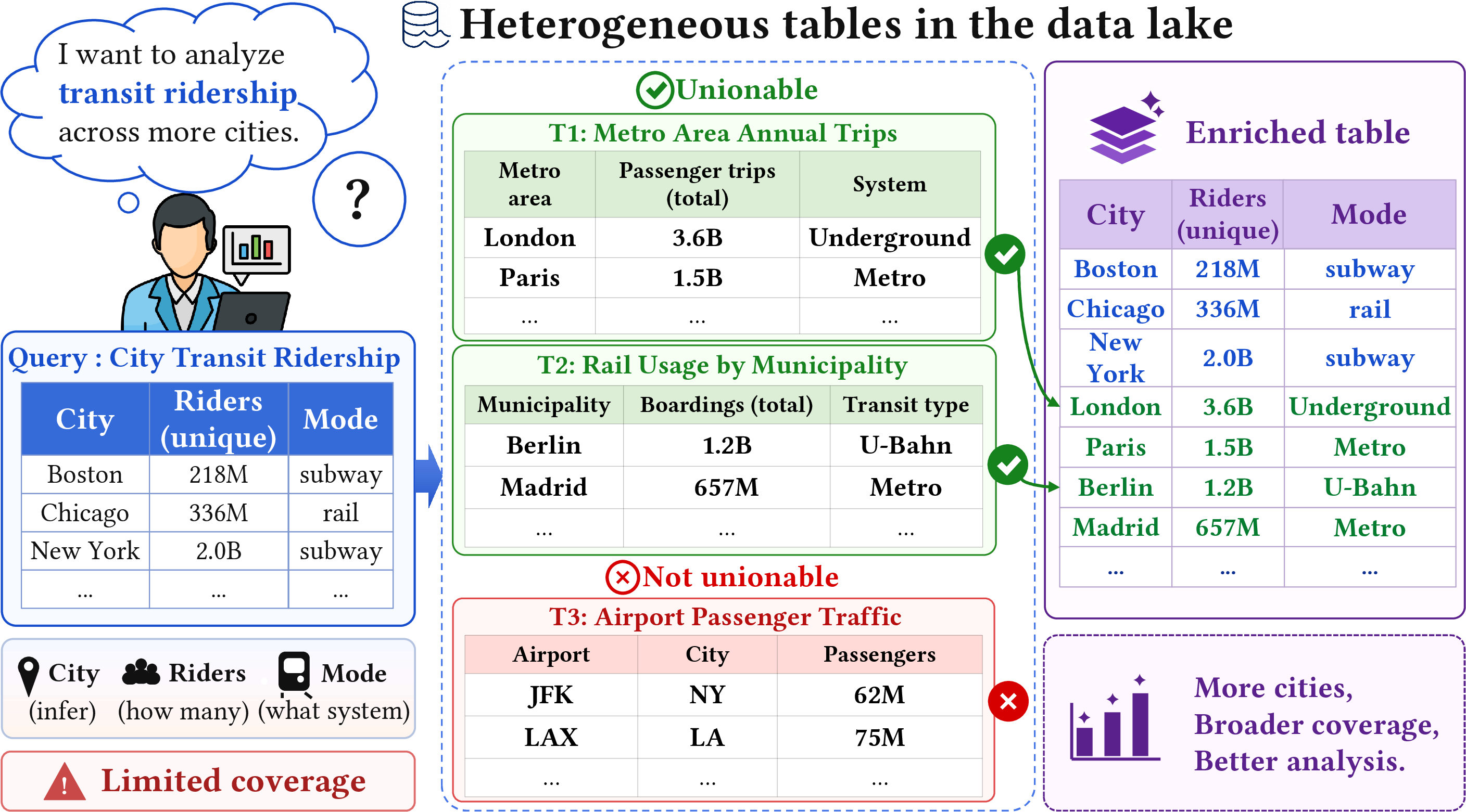
This need motivates table union search (TUS), which retrieves tables from a data lake that can be unioned with a given query table. TUS is a key primitive for data discovery, integration, enrichment, exploratory analysis, and downstream analytics or model training [8]–[11]. At its core, TUS is a semantic compatibility problem: it seeks tables whose columns can be aligned with the query table so that their rows can be appended. Unlike keyword-based table search or join-oriented discovery, unionability cannot be determined from keyword overlap or shared keys alone, because unionable tables may use different column names, have missing metadata, and share only sparse value overlap.
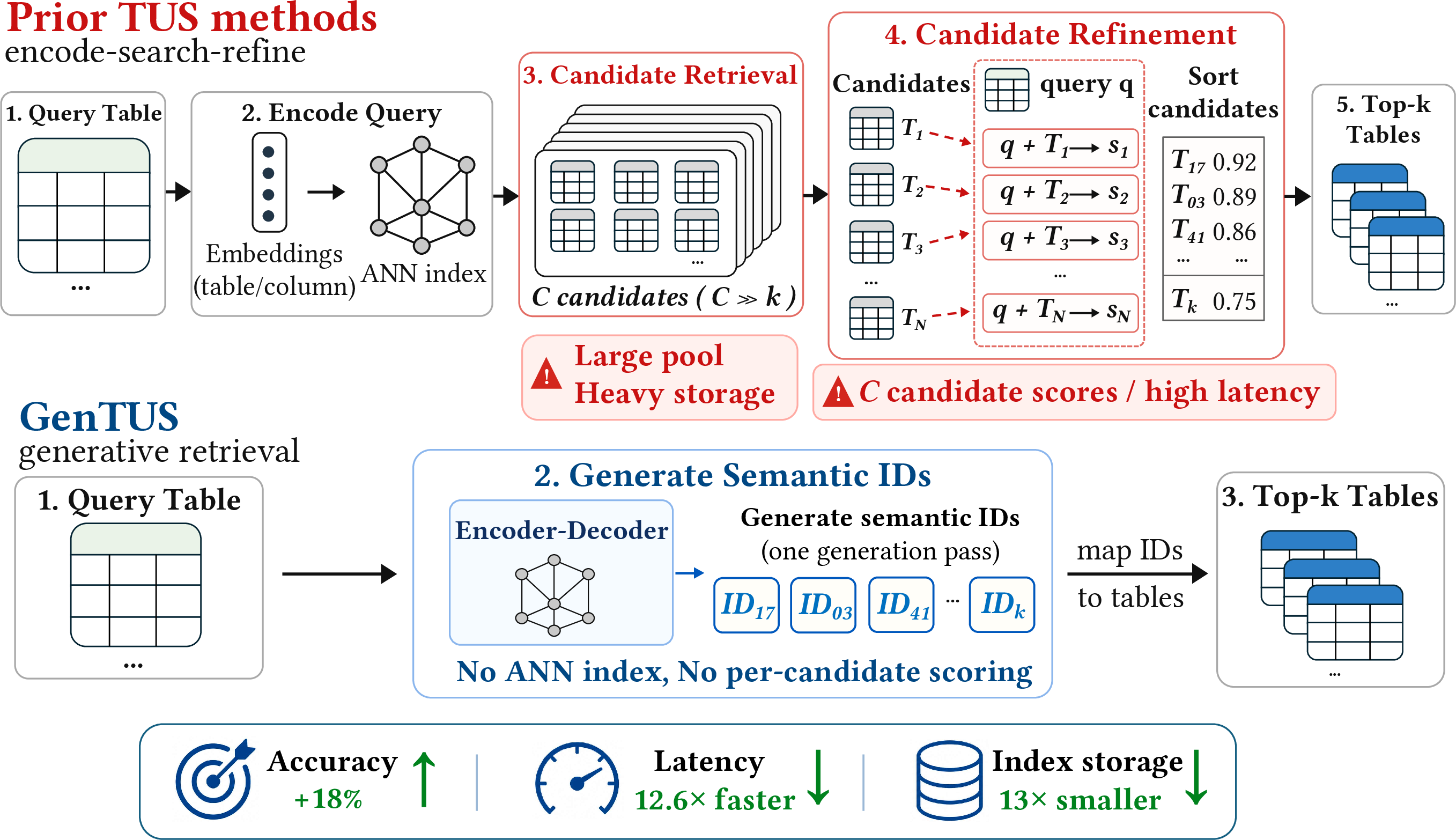
Prior works. As summarized in Figure 2, existing TUS methods largely follow an encode–search–refine pipeline. Specifically, they typically consist of three stages: (1) encoding, where tables or their components, such as columns, are encoded into dense representations; (2) index construction, where the resulting table or column embeddings are stored in a vector database to support efficient retrieval; and (3) online search and refinement, where the encoded query retrieves candidate tables through table-level search or column-level matches. The retrieved candidates are then refined by a reranking model or a matching-based scoring procedure to produce the final top-\(k\) unionable tables. Generally, different TUS methods mainly differ in the encoding and refinement stages. For example, Starmie [12] and LIFTus [13] encode each table at the column level and aggregate column-level evidence during retrieval or refinement to score candidate tables. In contrast, table-centric methods such as TACTUS [14] learn table-level embeddings for table-first candidate retrieval, followed by reranking with column-level evidence.
Motivation. Although the above pipeline works well when the data lake is small and clean, its limitations become clear when the lake becomes large and heterogeneous. First, the final result is highly dependent on the recall of the first-stage retrieval. If a truly unionable table is not retrieved as a candidate, the later refinement step has no chance to recover it. This becomes more serious in large data lakes, where many tables may be semantically close to the query and are difficult to separate using dense representations alone. Second, the online cost increases with the size of the data lake. For every query table, existing methods need to search the index, retrieve a candidate set, and then compare or rerank these candidates with the query table. As the lake grows, this query-time search-and-refine process becomes increasingly expensive. Third, existing methods also introduce large storage overhead. They need to store table or column embeddings, maintain search indexes, and sometimes keep additional structures for refinement or matching. These costs can be substantial for large data lakes. These limitations motivate us to ask a different question: Can we improve TUS quality and efficiency without explicitly searching and refining a candidate pool from a growing data lake?
Our technical contributions. We propose GenTUS, a generative table union search framework that, as shown in Figure 2, reformulates TUS as constrained generation over discrete semantic table identifiers. During retrieval, GenTUS generates target table identifiers directly via beam search over a prefix tree, eliminating the need for vector indexes, ANN search, or reranking models. This paradigm shift avoids explicit lake-wide ANN search and query–candidate reranking at inference time and eliminates the storage overhead of maintaining embeddings and retrieval indexes. The framework is built around two core designs.
The first design is unionability-aware semantic identifier construction. A content-only identifier construction approach minimizes reconstruction error and quantizes each table independently, leaving the codebook unaware of inter-table unionability relationships; since unionability is defined by pairwise annotations and cannot emerge from single-table content alone, the discrete identifier space lacks aggregated structure favorable for generating unionable tables. To address this, we incorporate a contrastive loss supervised by pairwise unionability annotations into training, explicitly guiding unionable table pairs to receive identifiers that share coarse structure in the discrete space. As a result, beam search is inclined to prioritize identifiers of unionable tables, without requiring a separate reranking stage.
The second design is SID-tree-based constrained decoding and online retrieval. Without structural constraints, the generator may spend beam capacity on identifiers that do not correspond to any candidate table. To address this, we organize all valid identifiers into a prefix tree and impose prefix constraints during decoding, ensuring that every generated identifier maps to an existing table in the data lake. Online retrieval then reduces to constrained beam search over the SID tree, with the decoding budget governed by beam width and identifier depth rather than explicit search over the data lake; inserting a new table requires only a local update to the SID tree without rebuilding any index.
Extensive experiments on seven public TUS benchmarks demonstrate that GenTUS substantially outperforms existing methods in retrieval quality, achieving an average rank of 1.05 compared to 2.57 for the strongest baseline TACTUS, while also outperforming encode–search–refine methods across offline build time, online retrieval latency, and index storage.
In summary, our main contributions are as follows.
We propose GenTUS, the first generative retrieval framework for TUS, reformulating table union search as constrained generation over discrete semantic table identifiers.
We design unionability-aware identifier construction that incorporates pairwise unionability supervision, so that unionable tables receive generation-friendly identifiers with shared coarse structure.
We propose prefix-tree-based constrained decoding that guarantees valid identifier generation and avoids explicit lake-wide candidate search during online retrieval.
We conduct experiments on seven public TUS benchmarks, demonstrating GenTUS’s advantages in retrieval quality and system efficiency over state-of-the-art methods.
Outline. We introduce the preliminaries in Section 2 and review related work in Section 3. We present an overview of GenTUS in Section 4, and detail the offline and online phases in Sections 5 and 6. Experimental results are reported in Section 7, and we conclude in Section 8.
2 Preliminaries↩︎
2.1 Table Union Search↩︎
Let \(\mathcal{D}=\{T_1,\ldots,T_N\}\) denote the candidate data lake, where each table \(T_i\) consists of a set of columns \(C_i\) and a collection of tuples defined over \(C_i\). Given a query table \(q\), table union search aims to retrieve a ranked list of candidate tables from \(\mathcal{D}\) that are unionable with \(q\). Following prior work [8], [9], [12], [14], we treat unionability as a semantic relation between tables rather than a strict schema-matching problem: two tables may be unionable even when their column names, schemas, or metadata differ, as long as their columns can be aligned under compatible semantics. We write \(\mu(q,T)\) for a unionability score between \(q\) and a candidate \(T\), with larger values indicating stronger unionability.
Definition 1 (Top-\(k\) Table Union Search). Following the standard TUS formulation [8], [9], given a data lake \(\mathcal{D}\), a query table \(q\), and a positive integer \(k\), top-\(k\) table union search returns a ranked list of \(k\) distinct tables \(\pi_k(q,\mathcal{D})=(T_{(1)},\ldots,T_{(k)})\) ordered by a unionability score \(\mu\): \(\mu(q,T_{(j)})\ge\mu(q,T_{(j+1)})\) for \(j=1,\ldots,k-1\).
We partition the annotated pairs \(\mathcal{G}\subseteq\mathcal{Q}\times\mathcal{D}\) into a training split \(\mathcal{G}_{\mathrm{train}}\subseteq\mathcal{Q}_{\mathrm{train}}\times\mathcal{D}\) and a test split \(\mathcal{G}_{\mathrm{test}}\subseteq\mathcal{Q}_{\mathrm{test}}\times\mathcal{D}\), where \(\mathcal{Q}_{\mathrm{train}}\cap\mathcal{Q}_{\mathrm{test}}=\emptyset\); all annotation-dependent offline training signals use only \(\mathcal{G}_{\mathrm{train}}\).
2.2 Generative Retrieval↩︎
In this paper we study a generative formulation of table union search. Each candidate table \(T_i\in\mathcal{D}\) is assigned a discrete semantic identifier \(s_i=(s_{i,1},\ldots,s_{i,\ell_i})\), with tokens drawn from a finite code vocabulary. In our implementation, \(s_i\) consists of an \(L\)-token residual-quantized base code, optionally followed by a suffix token for collision resolution. Let \(\mathcal{S}_\mathcal{D}=\{s_i\mid T_i\in\mathcal{D}\}\) be the set of valid identifiers under the current candidate data lake, and \(\phi:\mathcal{S}_\mathcal{D}\to\mathcal{D}\) the bijective mapping from identifiers back to tables.
Definition 2 (Generative TUS Retriever). A generative TUS retriever models the conditional probability \(p_\theta(s\mid q)\) of an identifier given the query table. At inference, it decodes identifiers from \(\mathcal{S}_\mathcal{D}\) and returns the corresponding tables through the mapping \(\phi\), producing the top-\(k\) result of Definition 1 in generation order.
3 Related Work↩︎
3.1 Table Discovery and Table Union Search↩︎
Table discovery aims to find useful tables from large data lakes for downstream analysis, integration, and enrichment. Different discovery intents have led to keyword or dataset search [15], schema matching, joinable-table discovery [2], [6], and unionable-table discovery. Early table discovery systems often rely on metadata, column headers, schemas, value overlap, semantic annotations, or hand-crafted similarity aggregation [16]–[20], although these signals can be unreliable in open data lakes, where datasets may lack predefined schemas and published metadata is often incomplete or inconsistent with the underlying data [1], [11], [20]. Recent benchmarks such as LakeBench [7] and end-to-end systems such as LakeCompass [21] have further advanced large-scale evaluation and deployment of table discovery systems.
Among these tasks, table union search (TUS) focuses on retrieving tables that can extend a query table with additional rows under compatible column semantics [1], [8], [22]–[24]. Unlike keyword search, where relevance is largely determined by textual similarity, TUS requires reasoning about semantic compatibility between tables. It also differs from joinable-table discovery, which seeks tables connected through join keys, whereas TUS aims to identify tables describing compatible attributes even when schemas, column names, or metadata differ.
3.2 Embedding-Based Table Union Search↩︎
To retrieve unionable candidates under schema and metadata heterogeneity, recent TUS methods increasingly rely on learned table or column embeddings. These methods build on broader advances in table representation learning [25], including TaBERT [26], TaPas [27], and TURL [28]. Beyond learned embeddings, prior work also exploits semantic type information [29], [30], relationship semantics [9], and schema-, value-, embedding-, or matching-based signals [17], [18], [31]–[33] to estimate table relatedness and unionability. Column-centric systems such as Starmie [12] and LIFTus [13] represent tables through contextualized or multi-aspect column embeddings, and aggregate column-level evidence to score candidate tables. More recent table-centric systems such as TACTUS [14] learn table-level embeddings for table-first candidate retrieval, followed by dual-evidence reranking with column-level signals. Despite differences in representation design, these methods share an embedding-based encode–search–refine pipeline: they encode tables or columns into dense representations, organize them in a search index, often an ANN index such as HNSW [34], retrieve candidate tables through table-level search or column-level matches, and then score or refine the candidates through matching, aggregation, or reranking. Rather than retrieving candidates through nearest-neighbor search and refining them post hoc, GenTUS directly generates identifiers of unionable tables under constrained decoding.
3.3 Generative Retrieval↩︎
Generative retrieval formulates retrieval as sequence generation over discrete candidate identifiers. Early differentiable search index and autoregressive retrieval methods show that entity retrieval can be cast as generating target identifiers conditioned on a query [35]–[38]. This paradigm has been especially influential in recommendation, where systems such as TIGER construct residual-quantized item identifiers and train sequence models to generate relevant item IDs [39], [40]. Subsequent work further improves item tokenization, collaborative-semantic alignment, and ranking-oriented training [41]–[44]. In data management, Birdie [45] brings differentiable search indexes to natural-language-driven table discovery, showing that an encoder–decoder index can unify table indexing and search, strengthen query–table interaction, and support continual table indexing.
Together, these works position generative retrieval as a promising interface for retrieving structured objects, including tables. However, applying this paradigm to TUS is non-trivial: generated identifiers and decoding scores must reflect table-pair unionability, rather than generic query–item relevance. GenTUS addresses this requirement through unionability-aware semantic identifiers and ranking-calibrated constrained generation.
4 Overview↩︎
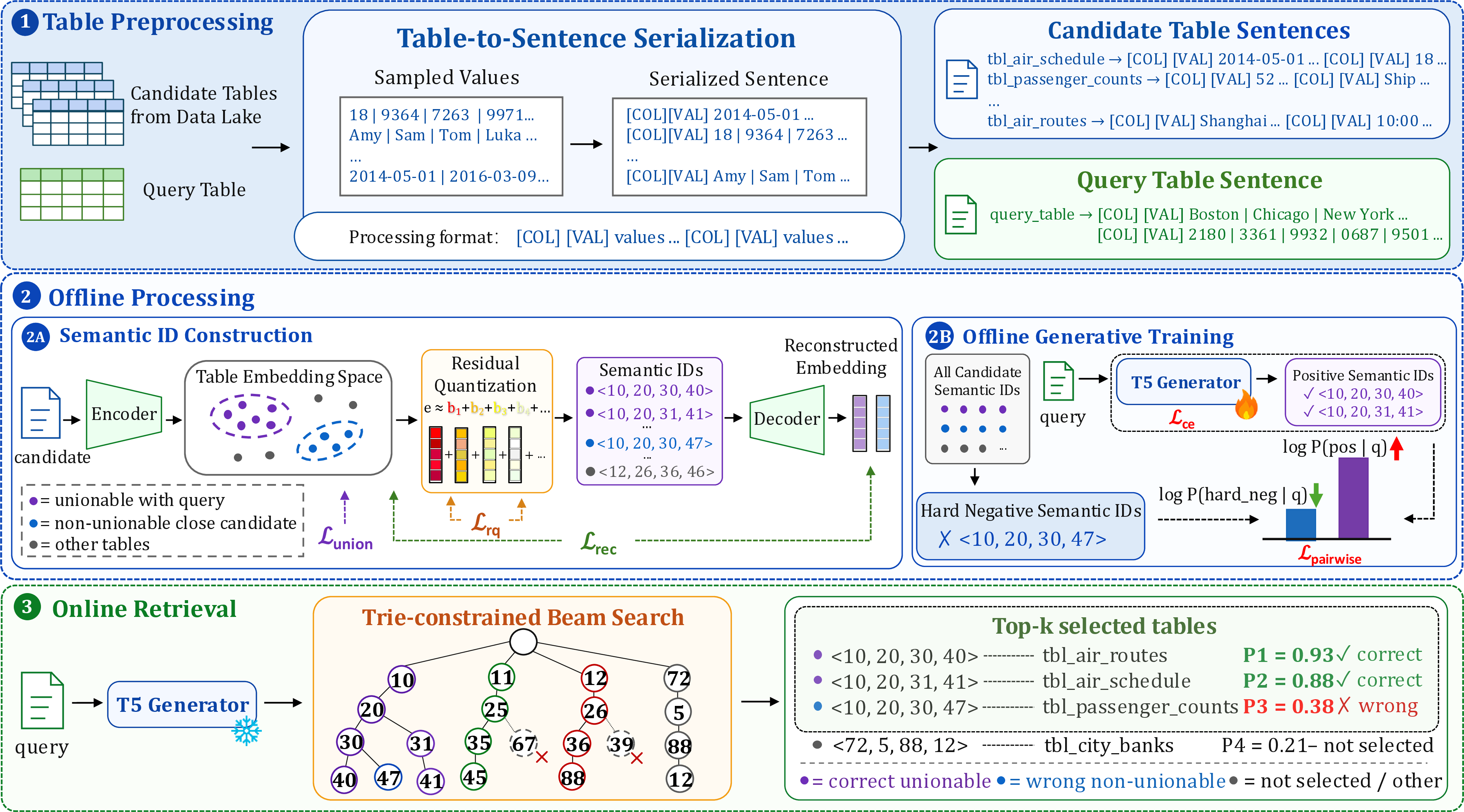
Figure 3 illustrates the overall framework of GenTUS. GenTUS reformulates table union search as constrained generation over semantic table identifiers. Instead of maintaining a dense vector index and retrieving candidates by nearest-neighbor lookup, GenTUS makes each candidate table addressable by a discrete semantic identifier. Given a query table, an encoder–decoder generator directly produces identifiers of candidate tables that are likely to be unionable with the query, and the generated identifiers are mapped back to data-lake tables as retrieval results.
Table preprocessing. GenTUS serializes both candidate and query tables into table sentences that compactly capture sampled cell values and column-level structure, without using column names. This shared format feeds the offline table representation step in Section 5.1 and is reused for generator inputs during training and online retrieval.
Offline processing. Given a data lake \(\mathcal{D}\), GenTUS constructs the generative search space in two parts. The first part defines the discrete identifier space for candidate tables, and the second part trains a generator to search this space from a query table.
First, GenTUS encodes candidate tables into table-level representations and performs unionability-aware semantic ID construction, as detailed in Section 5.1 and Section 5.2. For each candidate table \(T \in \mathcal{D}\), GenTUS feeds its serialized table sentence into a table encoder to obtain a table-level embedding, and then converts the embedding into a compact semantic identifier using a unionability-aware residual quantizer with learnable codebooks. The quantizer is trained to preserve table content while shaping the discrete identifier space according to table-pair unionability, so that unionable tables are encouraged to share coarse codes and occupy nearby regions of the identifier space. This step produces the valid identifier set \(\mathcal{S}_{\mathcal{D}}\), an identifier–table mapping \(\phi\), and a prefix tree \(\mathsf{Trie}_{\mathcal{D}}\) built over \(\mathcal{S}_{\mathcal{D}}\) for constrained decoding.
Second, GenTUS builds query-to-identifier training records and performs offline generative training, as detailed in Section 5.3 and Section 5.4. It trains an encoder–decoder generator \(G_\theta\) over query-to-identifier records derived from \(\mathcal{G}_{\mathrm{train}}\). Each record takes a serialized training query table as input and uses the semantic identifier of an annotated unionable candidate as the target output sequence. Besides the sequence generation objective, GenTUS further uses mined hard-negative identifiers and a pairwise ranking objective to calibrate the relative scores of positive and negative identifiers.
Online retrieval. Given a query table \(q\), GenTUS serializes \(q\) using the same generator preprocessing procedure and feeds it into the trained generator, as described in Section 6.1. The decoder generates semantic identifiers token by token. At each decoding step, the prefix tree \(\mathsf{Trie}_{\mathcal{D}}\) restricts the next token to prefixes that can still lead to an existing table identifier in \(\mathcal{S}_{\mathcal{D}}\). This trie constraint prevents invalid identifiers from consuming beam-search capacity. Completed identifiers are scored by the generator, mapped back to tables through \(\phi\), deduplicated, and returned as the top-\(k\) unionable tables.
5 Offline Processing↩︎
The offline stage builds the generative candidate space used by GenTUS and trains the retrieval generator. It consists of two conceptual steps: Sections 5.1–5.2 construct semantic identifiers for candidate tables, while Sections 5.3–5.4 train a generator that maps query tables to identifiers of unionable candidates.
5.1 Table Representation↩︎
Following the metadata-agnostic table-centric design of TACTUS [14], GenTUS first derives contextualized column representations from serialized cell values and then attention-pools them into a table embedding.
Under a bounded serialization budget, GenTUS retains all columns of each table and controls the input length by bounding the number of serialized values per column. For a table \(T\) with ordered columns \(C_T=(c_1,\ldots,c_{|C_T|})\), let \(V_j=(v_{j,1},\ldots,v_{j,r_j})\) be a bounded sequence of distinct non-empty values from column \(c_j\). The column and table serializations are \[\sigma_j=[\mathrm{COL}]\circ[\mathrm{VAL}]\circ \operatorname{tok}(v_{j,1})\circ \cdots \circ \operatorname{tok}(v_{j,r_j}).\] \[x_T=[\mathrm{CLS}]\circ\sigma_1\circ\cdots\circ\sigma_{|C_T|},\qquad \mathbf{H}_T = \mathrm{LM}_\eta(x_T),\] where \(|C_T|\) is the number of columns in table \(T\), \(\operatorname{tok}(\cdot)\) denotes tokenization, \(\circ\) denotes concatenation, and \(\mathrm{LM}_\eta\) is a pretrained encoder. Let \(p_j\) denote the position of the \([\mathrm{COL}]\) token for column \(c_j\) in \(x_T\). We use the encoder hidden state at \(p_j\) as the representation of column \(c_j\): \(\mathbf{h}^{\mathrm{col}}_{T,j}=\mathbf{H}_T[p_j]\). Stacking all column representations gives \(\mathbf{H}^{\mathrm{col}}_T=[\mathbf{h}^{\mathrm{col}}_{T,1};\ldots;\mathbf{h}^{\mathrm{col}}_{T,|C_T|}]\). A global query \(\mathbf{q}_\eta\) attention-pools the column representations into a table-level representation: \[\mathbf{h}^{\mathrm{tab}}_T = \operatorname{MultiHeadAttn}_\eta (\mathbf{q}_\eta,\mathbf{H}^{\mathrm{col}}_T,\mathbf{H}^{\mathrm{col}}_T).\] The table-level representation is then projected and normalized as the table embedding: \[\mathbf{e}_T = \frac{g_\eta(\mathbf{h}^{\mathrm{tab}}_T)}{\|g_\eta(\mathbf{h}^{\mathrm{tab}}_T)\|_2}.\] This continuous table embedding \(\mathbf{e}_T\) is then quantized into a discrete semantic identifier in the next step.
5.2 Semantic Identifier Construction↩︎
Design goals. GenTUS represents each candidate table with a semantic identifier so that table retrieval can be formulated as sequence generation over a finite identifier space. A useful identifier should satisfy two requirements: it should be compact enough to be generated reliably by an autoregressive decoder, and it should preserve the semantic structure needed for TUS so that unionable tables are placed close together in the identifier space.
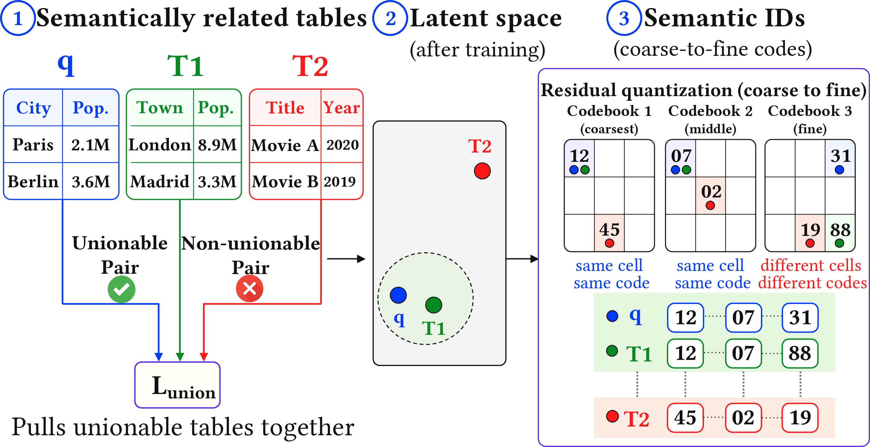
To this end, GenTUS constructs identifiers with residual quantization. Given the table embedding from Section 5.1, the quantizer maps each candidate table to a discrete sequence of code indices. Because residual quantization represents a vector through multiple codebooks, the resulting identifier provides a compact coarse-to-fine code sequence that can be generated by the retrieval generator. However, this quantization process by itself does not explicitly optimize identifiers for unionability. GenTUS therefore augments residual quantization with a unionability-aware contrastive objective, which pulls annotated unionable tables together in the quantizer latent space before discretization. As illustrated in Figure 4, this objective and the residual quantizer jointly encourage unionable tables to share coarse codes while still allowing finer codes to distinguish individual tables.
Residual quantization. Let \(\mathcal{Q}_{\mathrm{train}}\) and \(\mathcal{G}_{\mathrm{train}}\) be the training queries and training annotations defined in Section 2.1. The quantizer is fitted over candidate tables in \(\mathcal{D}\), and its unionability term is supervised by \(\mathcal{G}_{\mathrm{train}}\). For each table \(T_i\in\mathcal{D}\), we write \(\mathbf{e}_i\) as shorthand for its table embedding \(\mathbf{e}_{T_i}\) from Section 5.1.
The quantizer first maps this table embedding into a separate latent space used for code selection. An MLP encoder \(f_\omega\) produces the normalized quantizer latent vector \[\mathbf{z}_i = \frac{f_\omega(\mathbf{e}_i)}{\|f_\omega(\mathbf{e}_i)\|_2}.\] The latent vector is quantized by \(L\) residual codebooks \(\{\mathcal{B}_\ell\}_{\ell=1}^L\), where \(\mathcal{B}_\ell=\{\mathbf{b}_{\ell,1},\ldots,\mathbf{b}_{\ell,K}\}\). Starting from \(\mathbf{r}_i^{(0)}=\mathbf{z}_i\), the \(\ell\)-th code index is selected by nearest-neighbor lookup: \[a_{i,\ell}=\arg\min_{k}\left\|\mathbf{r}_i^{(\ell-1)}-\mathbf{b}_{\ell,k}\right\|_2^2,\] and the residual is updated as \(\mathbf{r}_i^{(\ell)}=\mathbf{r}_i^{(\ell-1)}-\mathbf{b}_{\ell,a_{i,\ell}}\). The selected codewords are summed to form the quantized latent vector \[\widehat{\mathbf{z}}_i = \sum_{\ell=1}^{L}\mathbf{b}_{\ell,a_{i,\ell}}.\] The corresponding code indices form the base semantic identifier \(\bar{s}_i=(a_{i,1},\ldots,a_{i,L})\) of candidate table \(T_i\).
Unionability-aware training and collision resolution. The quantizer is trained with three complementary objectives: a reconstruction loss, a residual quantization loss, and a unionability-aware contrastive loss. For reconstruction, a decoder \(g'_\omega\) maps the quantized latent vector back to the table-embedding space as \(\widehat{\mathbf{e}}_i=g'_\omega(\widehat{\mathbf{z}}_i)\). The reconstruction loss compares this reconstructed table embedding with the original table embedding: \[\mathcal{L}_\mathrm{rec} = \frac{1}{|\mathcal{D}|} \sum_{T_i\in\mathcal{D}} \left\|\mathbf{e}_i-\widehat{\mathbf{e}}_i\right\|_2^2.\]
The residual quantization loss \(\mathcal{L}_\mathrm{rq}\) trains the codebooks to represent the residual inputs at each level. Since nearest-neighbor codeword selection is non-differentiable, we follow the standard straight-through training of [40], [46] with a codebook term and a commitment term: \[\mathcal{L}_\mathrm{rq}=\frac{1}{|\mathcal{D}|}\sum_{T_i\in\mathcal{D}}\sum_{\ell=1}^{L}\Big(\mathcal{L}^{(\ell)}_{\mathrm{codebook}}(i)+\beta\mathcal{L}^{(\ell)}_{\mathrm{commit}}(i)\Big).\]
GenTUS further adds the unionability-aware contrastive objective over the latent vectors that pulls annotated unionable pairs together and contrasts them against other in-batch tables, aligning the identifier space with TUS semantics [47]. Let \(\mathcal{G}_{\mathrm{train}}\) denote the unionability annotations available in the training split, where \((q,T^+)\in\mathcal{G}_{\mathrm{train}}\) indicates that candidate table \(T^+\) is unionable with query table \(q\). For contrastive training, we use only observed training query–candidate annotations whose query anchor is available in the benchmark corpus, and symmetrize these query–candidate pairs without inferring additional positive relations. Let \(\mathcal{P}\) be the resulting symmetrized set of positive pairs.
For a mini-batch \(B\), let \(\mathcal{P}_i^B=\{j\in B\setminus\{i\}:(i,j)\in\mathcal{P}\}\) be the positives of table \(T_i\) within the batch. Mini-batches are sampled with positive-pair awareness so that annotated positive pairs are likely to appear in the same batch. The unionability objective is \[\mathcal{L}_\mathrm{union}=-\frac{1}{|\mathcal{I}_B|}\sum_{i\in\mathcal{I}_B}\frac{1}{|\mathcal{P}_i^B|}\sum_{j\in\mathcal{P}_i^B}\log\frac{\exp(\mathbf{z}_i^\top\mathbf{z}_j/\tau)}{\sum_{a\in B\setminus\{i\}}\exp(\mathbf{z}_i^\top\mathbf{z}_a/\tau)},\] where \(\mathcal{I}_B=\{i:\mathcal{P}_i^B\neq\emptyset\}\) and \(\tau\) is a temperature.
The full semantic-identifier training objective is \[\mathcal{L}_\mathrm{SID}=\mathcal{L}_\mathrm{rec}+\mathcal{L}_\mathrm{rq}+ \lambda_u\mathcal{L}_\mathrm{union},\] where \(\mathcal{L}_\mathrm{rec}\) and \(\mathcal{L}_\mathrm{rq}\) preserve the table-to-latent reconstruction and quantization behavior, while \(\mathcal{L}_\mathrm{union}\) shapes the latent space so that unionable tables receive identifiers with shared coarse codes.
Since residual quantization maps a continuous space to a finite code space, multiple candidate tables may receive the same base identifier. GenTUS resolves such collisions by defining the final semantic identifier as \[\operatorname{sid}(T_i)= \begin{cases} \bar{s}_i, & \text{if } \bar{s}_i \text{ is unique},\\ \bar{s}_i\circ[\mathrm{SUF}_{h_i}], & \text{if } \bar{s}_i \text{ belongs to a collision group}, \end{cases}\] where \(h_i\) is a unique suffix index assigned to \(T_i\) within its collision group. This makes each final identifier unique while preserving the shared base identifier for collided tables. The valid identifier set is then \(\mathcal{S}_{\mathcal{D}}=\{\operatorname{sid}(T):T\in\mathcal{D}\}\), with bijection \(\phi:\mathcal{S}_{\mathcal{D}}\to\mathcal{D}\) used for generator training and online decoding.
5.3 Training Instance Construction↩︎
After semantic identifiers are assigned, GenTUS converts annotated query–candidate unionability pairs into identifier-level supervision for the retrieval generator. This subsection constructs positive generation records and augments them with structure-preserving query views, so the generator learns to output identifiers of annotated unionable candidates under incidental layout variations. It also builds indexing records that ground table contents to identifiers and hard-negative ranking records that provide pairwise ranking supervision.
Here, \(\operatorname{ser}(\cdot)\) denotes the table-to-sentence serializer used to construct generator inputs. Let \(\mathcal{Q}_{\mathrm{train}}\) be the training queries and let \(\mathcal{G}_{\mathrm{train}}\subseteq \mathcal{Q}_{\mathrm{train}}\times\mathcal{D}\) be the training annotations, where \((q,T^+)\in\mathcal{G}_{\mathrm{train}}\) means that candidate table \(T^+\) is unionable with training query \(q\). We write \(\mathcal{G}_{\mathrm{train}}(q)=\{T\in\mathcal{D}:(q,T)\in \mathcal{G}_{\mathrm{train}}\}\) for the annotated positives of \(q\).
Positive generation records. For each annotated pair \((q,T^+)\in\mathcal{G}_{\mathrm{train}}\), GenTUS serializes \(q\) as the generator input and uses the final identifier of \(T^+\) as the target output sequence: \[(x_q,y^+)=(\operatorname{ser}(q),\operatorname{tok}(\operatorname{sid}(T^+))).\] Thus, each unionability annotation is rewritten as a sequence-to-sequence record from a query table to the identifier of a unionable candidate.
Structural augmentation. GenTUS constructs additional query views by sampling rows and varying column orders. If \(\operatorname{Aug}(q)\) denotes the set of augmented views of \(q\), each view \(\widetilde{q}\in\operatorname{Aug}(q)\cup\{q\}\) keeps the same target identifier, yielding \((\operatorname{ser}(\widetilde{q}),y^+)\), where \(y^+=\operatorname{tok}(\operatorname{sid}(T^+))\). We use bounded augmentations so that each view preserves the main table semantics while varying incidental structure. The resulting original and augmented positive records form \(\mathcal{R}_{\mathrm{pos}}\).
Indexing records. GenTUS also constructs self-mapping records that map a table’s own content to its identifier: \[\bigl( \operatorname{ser}(T), \operatorname{tok}(\operatorname{sid}(T)) \bigr).\] These records are created for candidate tables that appear as annotated positives in \(\mathcal{G}_{\mathrm{train}}\). They ground semantic identifiers in table content, so the generator learns not only query-to-candidate supervision but also the basic content-to-identifier mapping. The resulting records form the indexing set \(\mathcal{R}_{\mathrm{idx}}\).
Hard-negative ranking records. Finally, GenTUS constructs hard-negative records for the pairwise ranking objective. For each training query \(q\), it computes a lightweight table profile from sampled non-empty cell-value tokens. Candidate tables in \(\mathcal{D}\setminus(\mathcal{G}_{\mathrm{train}}(q)\cup\{q\})\) are ranked by Jaccard similarity to \(q\), and the top-\(n_{\mathrm{neg}}\) tables are used as mined hard negatives [48]. For \(\widetilde{q}\in\operatorname{Aug}(q)\cup\{q\}\), a ranking record has the form \[(\operatorname{ser}(\widetilde{q}), y^+, y^-) = \left( \operatorname{ser}(\widetilde{q}), \operatorname{tok}(\operatorname{sid}(T^+)), \operatorname{tok}(\operatorname{sid}(T^-)) \right),\] where \(T^+\in\mathcal{G}_{\mathrm{train}}(q)\) and \(T^-\in\mathcal{D}\setminus(\mathcal{G}_{\mathrm{train}}(q)\cup\{q\})\). These mined negatives share surface features with the query but are not annotated as positives, making them useful for calibrating generator scores in the ranking objective. The resulting triples form \(\mathcal{R}_{\mathrm{pairwise}}\).
5.4 Generator Training↩︎
Given the identifier-level records constructed in Section 5.3, GenTUS trains a retrieval generator to map serialized query tables to semantic identifiers of unionable candidate tables. The training records provide two complementary supervision signals. Records in \(\mathcal{R}_{\mathrm{pos}}\cup\mathcal{R}_{\mathrm{idx}}\) are used with a token-level cross-entropy objective, which teaches the generator to produce valid target identifiers. Records in \(\mathcal{R}_{\mathrm{pairwise}}\) are used with a pairwise ranking objective, which encourages annotated positive identifiers to receive higher sequence scores than mined hard-negative identifiers [49]. This ranking objective operates over discrete identifier sequences and is distinct from \(\mathcal{L}_\mathrm{union}\) in semantic identifier construction (Section 5.2), which shapes the continuous latent space before quantization.
Generator parameterization. GenTUS instantiates the generator as a T5 encoder–decoder. Since the decoder must generate semantic identifiers rather than only natural-language tokens, GenTUS extends the tokenizer with identifier-specific tokens. Specifically, the tokenizer is extended with \(K\) code-index tokens shared across residual-code positions; the position of a token in the identifier sequence determines the corresponding residual codebook. This lets the same code-index vocabulary represent each residual-code level while preserving the ordered structure of the identifier. The tokenizer is also extended with suffix tokens for collision resolution and structural markers \([\mathrm{COL}]\) and \([\mathrm{VAL}]\) used by the generator serializer. All other tokens are inherited from the base T5 tokenizer.
Cross-entropy training. Given an input serialization \(x\) and an identifier sequence \(y\), where \(y=\operatorname{tok}(\operatorname{sid}(T))\) for some candidate table \(T\), the generator defines \[P_\theta(y\mid x)= \prod_{t=1}^{|y|} P_\theta(y_t\mid y_{<t},x).\] For a positive target identifier \(y^+\), the token-level cross-entropy loss is \[\mathcal{L}_\mathrm{ce}= -\frac{1}{|y^+|} \sum_{t=1}^{|y^+|} \log P_\theta(y^+_t\mid y^+_{<t},x).\] This loss is applied to positive generation records in \(\mathcal{R}_{\mathrm{pos}}\) and table-to-identifier indexing records in \(\mathcal{R}_{\mathrm{idx}}\).
Pairwise ranking training. For ranking, GenTUS scores an identifier sequence by its average conditional log-likelihood under the generator \[s_\theta(y\mid x)= \frac{1}{|y|} \sum_{t=1}^{|y|} \log P_\theta(y_t\mid y_{<t},x).\] Given a ranking triple \((x,y^+,y^-)\), where \(y^+\) is the identifier of an annotated positive candidate and \(y^-\) is the identifier of a mined hard-negative candidate, the pairwise ranking loss is \[\mathcal{L}_\mathrm{pairwise}= \max\left( 0, \gamma- s_\theta(y^+\mid x) + s_\theta(y^-\mid x) \right),\] where \(\gamma\) is the margin. This loss is applied to hard-negative ranking records in \(\mathcal{R}_{\mathrm{pairwise}}\) and calibrates the generator so that positive identifiers receive higher average sequence log-likelihood than hard-negative identifiers.
The full generator objective is \[\mathcal{L}_\mathrm{gen}= \mathcal{L}_\mathrm{ce} + \lambda_r \mathcal{L}_\mathrm{pairwise}.\] The cross-entropy term trains the generator to produce target identifiers, while the ranking term improves the relative ordering of positive and mined hard-negative identifiers under the model likelihood. During online retrieval, GenTUS does not perform a separate post-hoc query–candidate scoring step. Valid identifiers returned by prefix-constrained beam search are ranked by the beam-search order induced by the generator scores.
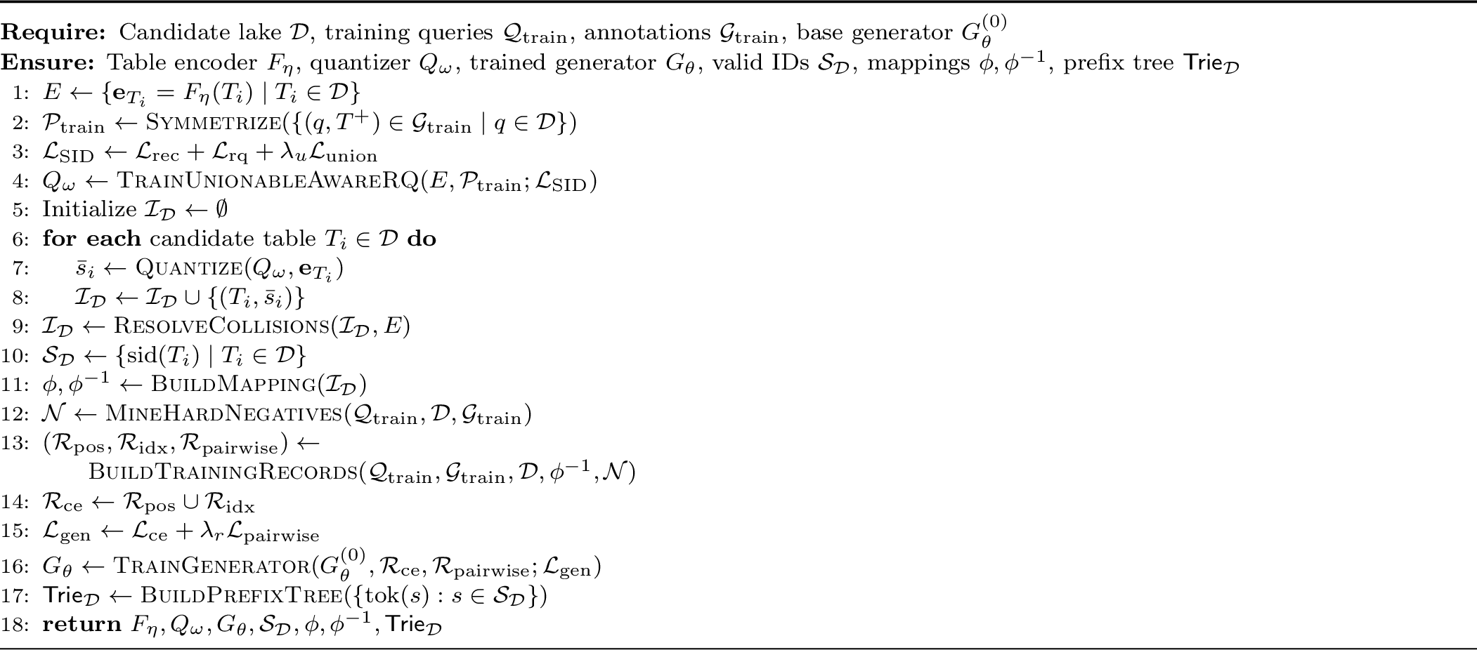
Offline pipeline summary. Algorithm 5 summarizes how the preceding components form the complete offline pipeline. Given the candidate lake, training queries, and unionability annotations, GenTUS first encodes candidate tables and constructs valid semantic identifiers, then rewrites training annotations into identifier-level records and trains the retrieval generator. The offline stage also produces the identifier mappings and prefix tree used by online constrained decoding.
6 Online Retrieval↩︎
The online stage uses the generator and identifier structures produced offline to retrieve unionable tables through generation. Given a query table, GenTUS serializes it as the generator input, performs prefix-constrained decoding over valid semantic identifiers, and maps the completed identifiers back to candidate tables (Section 6.1). Thus, online retrieval is formulated as constrained identifier generation rather than dense-index lookup followed by explicit query–candidate reranking. Section 6.2 describes how the valid identifier space is updated for newly added candidate tables without retraining the generator.
6.1 Constrained Identifier Generation and Ranking↩︎
Given a query table \(q\), GenTUS applies the same serializer used during offline training, \(x_q=\operatorname{ser}(q)\). The serialized query is fed into the trained encoder–decoder generator. For an identifier sequence \(s=(s_1,\ldots,s_{|s|})\), the generator defines the autoregressive probability \[P_\theta(s\mid x_q)=\prod_{t=1}^{|s|}P_\theta(s_t\mid s_{<t},x_q).\] Validity is enforced by the prefix-constrained decoding rule below.
Prefix-constrained decoding. The prefix tree \(\mathsf{Trie}_{\mathcal{D}}\) is the online validity structure of GenTUS. It stores the finite language of valid semantic identifiers under the current data lake, and constrains the decoder so that every completed sequence corresponds to an existing candidate table. This prevents beam search from spending capacity on invalid identifier sequences and makes the generated candidate space directly updatable when new identifiers are inserted.
It is constructed over the tokenized final identifier set \(\{\operatorname{tok}(s):s\in\mathcal{S}_{\mathcal{D}}\}\). For a decoded prefix \(y_{1:t}=(y_1,\ldots,y_t)\), GenTUS defines the valid next-token set as \[\begin{align} \mathcal{A}(y_{1:t}) =&\;\{v \mid y_{1:t}\circ v \text{ is a prefix in } \mathsf{Trie}_{\mathcal{D}}\} \\ &\;\cup \{\mathrm{EOS} \mid y_{1:t}=\operatorname{tok}(s),\;s\in\mathcal{S}_{\mathcal{D}}\}. \end{align}\] Continuation tokens are allowed only if they keep the decoded sequence on a valid identifier prefix, and \(\mathrm{EOS}\) is allowed whenever the current prefix already forms a complete valid identifier, even if that prefix also has valid suffix continuations.
At each decoding step, GenTUS masks invalid next tokens before the beam update. If \(\ell_\theta(v\mid y_{1:t},x_q)\) denotes the generator logit (i.e., pre-softmax score) for token \(v\), the constrained logit is \[\ell_\theta^{\mathrm{valid}}(v\mid y_{1:t},x_q)= \begin{cases} \ell_\theta(v\mid y_{1:t},x_q), & v\in\mathcal{A}(y_{1:t}),\\ -\infty, & v\notin\mathcal{A}(y_{1:t}). \end{cases}\] Beam search then expands only prefixes that remain valid under \(\mathsf{Trie}_{\mathcal{D}}\). The decoder returns a list of completed valid identifiers \[\mathcal{Y}_q=[s^{(1)},\ldots,s^{(M)}],\] where each \(s^{(m)}\in\mathcal{S}_{\mathcal{D}}\). GenTUS preserves the beam-search order induced by the constrained generator scores as the identifier ranking.
Table mapping and ranking. Prefix-constrained decoding returns an ordered list of valid identifiers \(\mathcal{Y}_q=[s^{(1)},\ldots,s^{(M)}]\), where each \(s^{(m)}\in\mathcal{S}_{\mathcal{D}}\). GenTUS maps these identifiers to candidate tables using \(\phi:\mathcal{S}_{\mathcal{D}}\to\mathcal{D}\): \[\widetilde{\mathcal{R}}_q = [\phi(s^{(1)}),\ldots,\phi(s^{(M)})].\] If duplicate tables appear after mapping, GenTUS keeps the earliest occurrence and removes later duplicates. Let \(\mathcal{R}_q\) denote the resulting deduplicated ordered list. The final top-\(k\) result is \[\pi_k(q,\mathcal{D}) = \operatorname{FirstK}_k(\mathcal{R}_q).\] The order of \(\mathcal{R}_q\) is inherited from the constrained beam search, so GenTUS uses it directly as the retrieval ranking without post-hoc query–candidate alignment scoring over an ANN-retrieved candidate pool. Algorithm 6 summarizes the online retrieval pipeline.

6.2 Updating the Candidate Space↩︎
Data lakes are often dynamic, with new tables added after offline training. In GenTUS, such updates only require adding new valid identifiers to the generative candidate space, rather than retraining the generator or rebuilding a dense index. When a new table \(T'\) is added, GenTUS encodes it with the existing table encoder and quantizes its embedding with the trained quantizer to obtain a base identifier. If this base identifier collides with an existing one, GenTUS appends a suffix token as in Section 5.2. The resulting final identifier is inserted into the valid identifier set \(\mathcal{S}_{\mathcal{D}}\), the identifier mapping \(\phi\), and the prefix tree \(\mathsf{Trie}_{\mathcal{D}}\), while all existing identifiers remain unchanged.
If the latent dimension is \(d_z\), the update cost for identifier assignment and trie insertion is \(O(LKd_z + |\operatorname{sid}(T')|)\), excluding the cost of table encoding. The first term comes from nearest-neighbor lookup over \(L\) residual codebooks of size \(K\) in the \(d_z\)-dimensional latent space, and the second term comes from inserting the tokenized identifier into the prefix tree. The generator parameters, quantizer encoder, and residual codebooks are kept fixed.
After the update, subsequent queries decode over the expanded valid identifier set, so the new table becomes reachable through prefix-constrained decoding. Thus, candidate-space updates are handled by updating the identifier mapping and decoding constraint structure, without re-encoding existing lake tables, retraining the generator, or rebuilding an ANN index.
7 Experiments↩︎
| Statistic | TUS-S | TUS-L | SAN-S | SAN-L | Wiki | LB-1K | LB-30K |
|---|---|---|---|---|---|---|---|
| #Tables | 1,530 | 5,043 | 550 | 11,090 | 40,752 | 7,970 | 7,970 |
| #Cols | 14,810 | 54,923 | 6,322 | 123,477 | 106,744 | 151,572 | 151,572 |
| Avg.#Cols | 9.7 | 10.9 | 11.5 | 11.1 | 2.6 | 19.0 | 19.0 |
| Avg.#Rows | 4,466 | 1,915 | 6,921 | 7,675 | 51 | 936 | 19,138 |
2.5pt
We evaluate GenTUS through five research questions.
RQ1 (Retrieval quality). Does GenTUS match or outperform state-of-the-art table union search methods on standard TUS benchmarks (Section 7.2)?
RQ2 (Efficiency and storage). Does GenTUS lower offline build time, online retrieval time, and index storage (Section 7.3)?
RQ3 (Incremental indexing). When new tables arrive, can GenTUS index them more efficiently while maintaining retrieval quality (Section 7.4)?
RQ4 (Robustness to candidate-space size). Does GenTUS maintain retrieval quality as the candidate pool scales to the full lake (Section 7.5)?
Table 2: Retrieval quality at each dataset’s standard \(k\), reporting MAP@k, P@k, R@k, and Avg. Rank over all dataset–metric pairs. reports mean/std over three runs; best results are in bold, and second-best results are underlined. Method TUS_small TUS_large SANTOS_small SANTOS_large wiki_union LakeBench_1k LakeBench_30k Avg. 2-4(lr)5-7(lr)8-10(lr)11-13(lr)14-16(lr)17-19(lr)20-22 MAP@k P@k R@k MAP@k P@k R@k MAP@k P@k R@k MAP@k P@k R@k MAP@k P@k R@k MAP@k P@k R@k MAP@k P@k R@k Rank Sherlock 0.970 0.974 0.333 0.736 0.741 0.167 0.874 0.884 0.713 0.301 0.304 0.414 0.105 0.187 0.157 0.368 0.164 0.595 0.364 0.161 0.588 5.00 LIFTus 0.972 0.977 0.334 0.989 0.992 0.237 0.962 0.941 0.702 0.453 0.357 0.467 0.347 0.254 0.209 0.107 0.054 0.193 0.109 0.053 0.191 4.38 SATO 0.976 0.979 0.335 0.929 0.942 0.224 0.850 0.870 0.701 0.331 0.339 0.449 0.160 0.224 0.192 0.364 0.165 0.596 0.373 0.163 0.591 4.12 Starmie 0.977 0.983 0.335 0.913 0.923 0.215 0.967 0.968 0.784 0.393 0.396 0.510 0.284 0.429 0.348 0.304 0.090 0.337 0.296 0.083 0.323 3.88 TACTUS 0.994 0.988 0.330 0.984 0.973 0.252 0.986 0.972 0.729 0.468 0.439 0.575 0.654 0.624 0.507 0.434 0.160 0.559 0.437 0.164 0.570 2.57 GenTUS 0.997 0.997 0.342 0.997 0.998 0.238 0.988 0.989 0.804 0.532 0.558 0.666 0.704 0.773 0.638 0.602 0.238 0.766 0.613 0.240 0.765 1.05 0.3pt
RQ5 (Ablation and analysis). Which components contribute most to GenTUS’s performance, and how does decoding affect the accuracy–latency trade-off (Section 7.6)?
7.1 Experimental Setup↩︎
Datasets. We evaluate on seven TUS datasets, summarized in Table 1: TUS_small, TUS_large, SANTOS_small, SANTOS_large, wiki_union, and two LakeBench-derived OpenData row-cap variants [7]. The two LakeBench variants share the same tables, queries, and ground truth, but cap each CSV table at \(1{,}000\) and \(30{,}000\) rows, respectively [7]. Together, the datasets cover a range of sizes, domains, and table-content scales. Each dataset is evaluated at its standard \(k\): 60 for TUS and LakeBench, 10 for SANTOS_small, 20 for SANTOS_large, and 40 for wiki_union.
Protocol. All training objectives (i.e., semantic identifier construction (\(\mathcal{L}_{\mathrm{union}}\)), generator training, and hard-negative mining) use only \(\mathcal{G}_{\mathrm{train}}\), following the partition in Section 2.1. At inference, each test query is decoded against \(\mathcal{S}_{\mathcal{D}}\); if the query table itself appears in the candidate pool, it is excluded from its own ranked list following standard TUS evaluation practice. For GenTUS, we repeat the main retrieval-quality experiment three times with different random seeds and report the mean and standard deviation in Table 2.
Baselines. We compare against two groups of baselines. The first is semantic-type-based: Sherlock [29] and SATO [30]. The second learns table or column representations for TUS. Starmie [12] and LIFTus [13] are column-centric, and TACTUS [14] is table-centric.
We apply the same reproduction policy to all baselines: we use public implementations when available, or faithful reimplementations otherwise, and keep each method’s recommended or best-reported configuration. For retrieval baselines, this includes the published candidate-space size, ANN/HNSW parameters, and reranking budget when applicable.
Metrics. Following prior TUS work [8], [9], [12], [22], we report Mean Average Precision at \(k\) (MAP@\(k\)), Precision at \(k\) (P@\(k\)), and Recall at \(k\) (R@\(k\)). For a query table \(q\), let \(\mathcal{G}(q)\) be its truly unionable tables and \(\mathcal{R}_k(q)\) the ranked top-\(k\) tables returned by a method. We define \(\mathrm{P}@k=\frac{|\mathcal{R}_k(q)\cap\mathcal{G}(q)|}{k}\) and \(\mathrm{R}@k=\frac{|\mathcal{R}_k(q)\cap\mathcal{G}(q)|}{|\mathcal{G}(q)|}\). For MAP@\(k\), we follow the standard TUS protocol: each ground-truth table \(g\in\mathcal{G}(q)\) contributes \(\mathrm{P}@r_q(g)\) if \(g\) appears in \(\mathcal{R}_k(q)\) at rank \(r_q(g)\), and contributes \(0\) otherwise; AP@\(k\) averages these contributions over \(\mathcal{G}(q)\), and MAP@\(k\) averages AP@\(k\) over all queries.
P@\(k\) measures the fraction of returned tables that are truly unionable, R@\(k\) measures the fraction of all ground-truth unionable tables retrieved within top-\(k\), and MAP@\(k\) measures whether ground-truth unionable tables are ranked early.
We also report each method’s average rank across all metrics and datasets. For system cost, the offline build time is the one-time cost to prepare reusable retrieval artifacts for a fixed candidate lake, including GenTUS identifiers and generator artifacts, and each baseline’s representations, indexes, caches, or features. Online time is the end-to-end time to answer all test queries; all methods run on the same hardware.
Implementation. The table encoder is BERT-base [50]. To align with prior TUS work that treats column names as missing or unreliable metadata in open data lakes, each table is serialized without column names, using all columns and up to 24 sampled values per column under a 512-token budget. Multi-head attention then pools the resulting column representations into one table vector. The semantic identifier uses a residual quantizer with \(L{=}6\) codebooks of size \(K{=}256\), with suffix tokens used only to disambiguate duplicate base codes. The quantizer is trained with a unionability-aware contrastive term of weight \(\lambda_u{=}0.1\) and temperature \(\tau{=}0.1\). The generator is a T5-base [51] encoder–decoder. We train it with cross-entropy and the pairwise ranking objective, using margin \(\gamma{=}0.2\) and weight \(\lambda_r{=}0.2\). Training runs for 30 epochs with batch size 32 and learning rate \(3{\times}10^{-4}\). Online decoding uses prefix-constrained beam search with beam width \(\max(2k,100)\). All experiments run on 8 NVIDIA A100-80GB GPUs.
7.2 Retrieval Quality↩︎
Table 2 reports MAP, P, and R at each dataset’s standard \(k\), along with the average rank across all metrics and datasets. For GenTUS, we additionally report the mean and standard deviation over three independent runs. GenTUS achieves the best mean result on almost every dataset and metric, with an average rank of \(1.05\)—\(1.5\) rank positions ahead of the runner-up TACTUS (\(2.57\)).

Near-ceiling benchmarks. On TUS_small, TUS_large, and SANTOS_small, most methods are already close to the ceiling, so the margins are small. On TUS_small, GenTUS reaches MAP \(99.7\%\), P \(99.7\%\), and R \(34.2\%\), exceeding the strongest overall baseline TACTUS by \(0.3\), \(0.9\), and \(1.2\) percentage points. On TUS_large, GenTUS leads in MAP (\(99.7\%\)) and P (\(99.8\%\)), while TACTUS attains the highest R (\(25.2\%\) versus GenTUS’s \(23.8\%\)). These lakes are semantically clean and small enough that all methods do well, and GenTUS still leads in average rank across all three benchmarks.
Larger and more diverse benchmarks. The advantage widens on SANTOS_large, wiki_union, and the two LakeBench splits, where larger scale and greater semantic diversity make retrieval more challenging. On SANTOS_large, GenTUS reaches P \(55.8\%\) and R \(66.6\%\), surpassing TACTUS by \(11.9\) and \(9.1\) percentage points; MAP also improves from \(46.8\%\) to \(53.2\%\). On wiki_union, GenTUS attains P \(77.3\%\) and R \(63.8\%\), exceeding TACTUS by \(14.9\) and \(13.1\) percentage points, with MAP rising from \(65.4\%\) to \(70.4\%\). On LakeBench_1k and LakeBench_30k, GenTUS attains about \(60\%\) MAP and about \(77\%\) R, while TACTUS reaches only about \(43\%\) MAP and \(56\%\) R—gaps of more than \(17\) percentage points in MAP and more than \(20\) percentage points in R.
On the larger and more diverse lakes, the baselines are more affected by their respective retrieval bottlenecks: type-based methods rely on coarse column categories, column-aggregation methods search over a much larger column space, and table-vector pipelines compress table evidence before retrieving a bounded candidate pool. GenTUS instead directly generates unionability-supervised semantic identifiers, preserving unionability signals through retrieval.
Varying \(k\). Figure 7 reports Precision@\(K\) and Recall@\(K\) as \(K\) grows. As expected, precision decreases for all methods as \(K\) grows. At every \(K\), GenTUS keeps the highest precision and recall, and its lead grows at larger \(K\). On TUS_small and TUS_large, its precision stays near \(0.99\) through \(K{=}100\), while the baselines drop to about \(0.6\). On larger and more diverse lakes such as wiki_union and LakeBench, GenTUS keeps improving recall toward near-complete coverage as \(K\) grows, whereas the baselines plateau early. These results show that the advantage of GenTUS holds across the full range of \(K\) rather than at any single operating point.
7.3 Efficiency and Storage↩︎
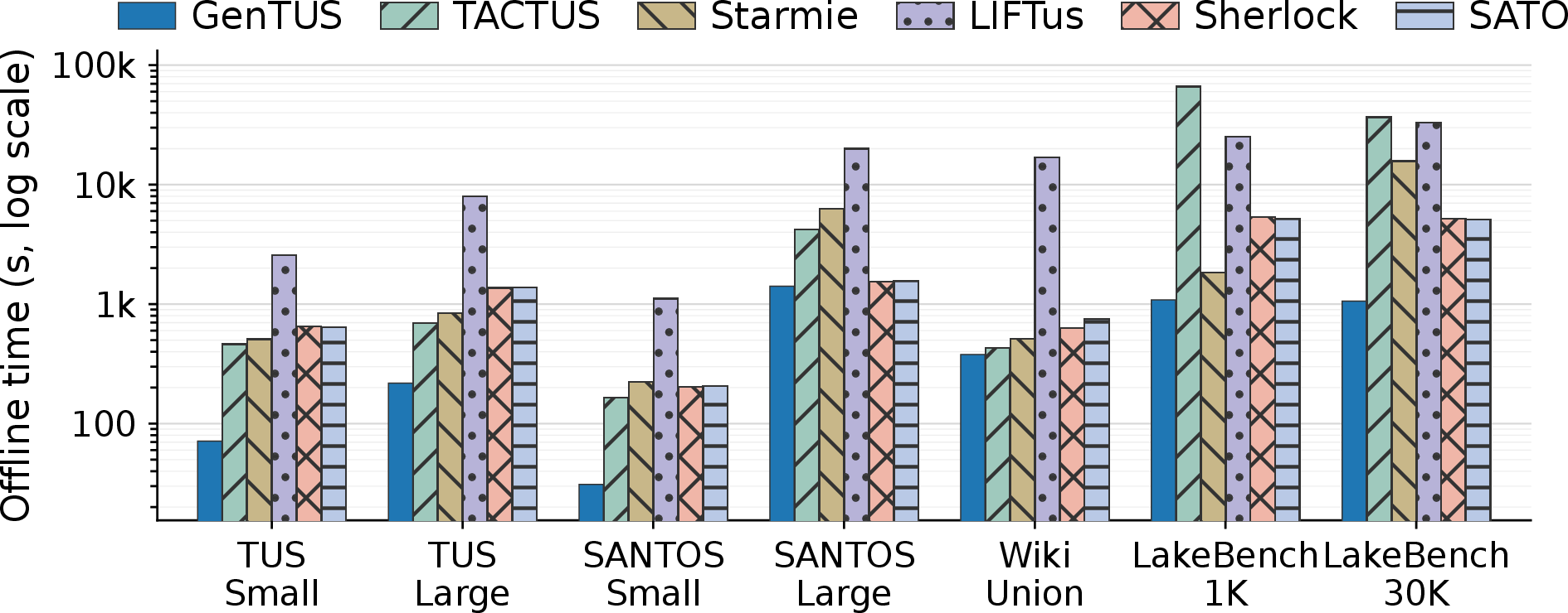
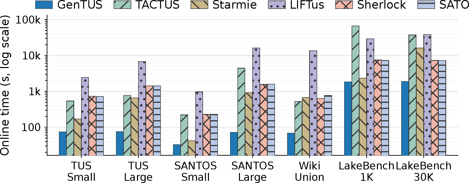
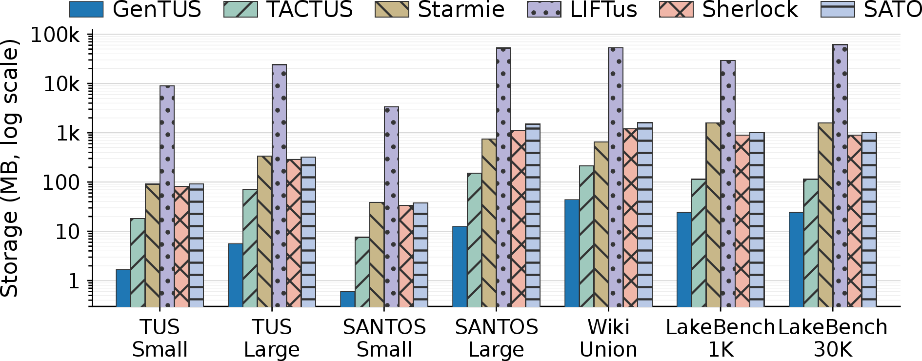
We report three system costs: offline build time (Figure 8), online end-to-end time (Figure 9), and retrieval-artifact storage (Figure 10). Across these measurements, GenTUS is consistently the most efficient method.
Offline. GenTUS has the lowest offline build time on every dataset. Compared with the fastest competing method on each dataset, GenTUS reduces offline build time by \(1.1\times\) to \(6.5\times\): on TUS_small it takes \(71\) seconds versus \(463\) for the next fastest baseline (\(6.5\times\)), and on SANTOS_large it takes \(1410\) seconds versus \(1534\) seconds. The gap is larger against some individual baselines: on the two LakeBench splits, TACTUS takes \(66204\) and \(36741\) seconds, while GenTUS finishes in about \(1060\) to \(1085\) seconds. This advantage comes from the compact retrieval artifacts used by GenTUS: after candidate tables are assigned discrete identifiers, online retrieval relies on the identifier mapping and prefix tree rather than dense vector indexes and per-candidate reranking artifacts.
Online. Figure 9 compares online end-to-end time on a log scale, where the GenTUS bars sit well below the others. GenTUS is fastest online on every dataset, between \(1.3\times\) and \(220\times\) faster than the fastest competing method on each dataset. On SANTOS_large it takes \(72.6\) seconds versus \(4434\) for TACTUS (\(61\times\)), and on LakeBench_1k it takes \(1,849\) seconds versus \(66,692\) seconds. This follows from replacing candidate lookup and per-candidate reranking with constrained identifier generation.
Storage. Figure 10 reports the storage size of retrieval artifacts maintained for each candidate lake, excluding fixed model weights. For GenTUS, these artifacts include the semantic identifiers, the identifier–table mapping , and the prefix tree used for constrained decoding. For embedding-based baselines, they include the stored embeddings, indexes, or other retrieval artifacts required for online search. GenTUS requires the least retrieval-artifact storage on every dataset. On SANTOS_large, these artifacts take \(12.6\) MB for GenTUS and \(746.6\) MB for Starmie, about \(59\times\) smaller. The gap is larger against LIFTus, whose retrieval artifacts reach tens of GB on the larger datasets.
| Method | TACTUS | Starmie | Sherlock | SATO | LIFTus | |
|---|---|---|---|---|---|---|
| Storage cost (MB) | 866 | 642 | 1,076 | 1,405 | 1,793 | \(>\!60{,}000\) |
2pt
To make the serving-time storage comparison explicit, Table 3 reports the total deployment footprint on wiki_union, including both the retrieval artifacts in Figure 10 and the model weights loaded at inference time. As a result, GenTUS requires 866 MB in total—below Starmie, Sherlock, SATO, and LIFTus, and only moderately above TACTUS (642 MB).
7.4 Incremental Indexing↩︎
Data lakes grow continuously as new tables arrive, so a practical method should admit new tables at low update cost. This experiment studies how each method indexes incoming tables, in terms of both the resulting retrieval quality and the cost of admitting new tables.
Protocol. We follow a strict \(D_0\)–\(D_5\) incremental protocol: all method-specific training and retrieval artifacts are built from \(D_0\) only, with \(D_1,\ldots,D_5\) introduced only at their update steps. \(D_0\) contains the initial 50% of tables, and each later split adds 10%. After every step, all queries are evaluated against the current active pool, in which the newly added tables are ranked together with the existing ones.
GenTUS ingests a new table by assigning it a semantic identifier and inserting it into the prefix tree, with the generator kept frozen. The dense-retrieval baselines update incrementally as well: each new table is encoded with the pre-trained encoder and inserted into the existing index.
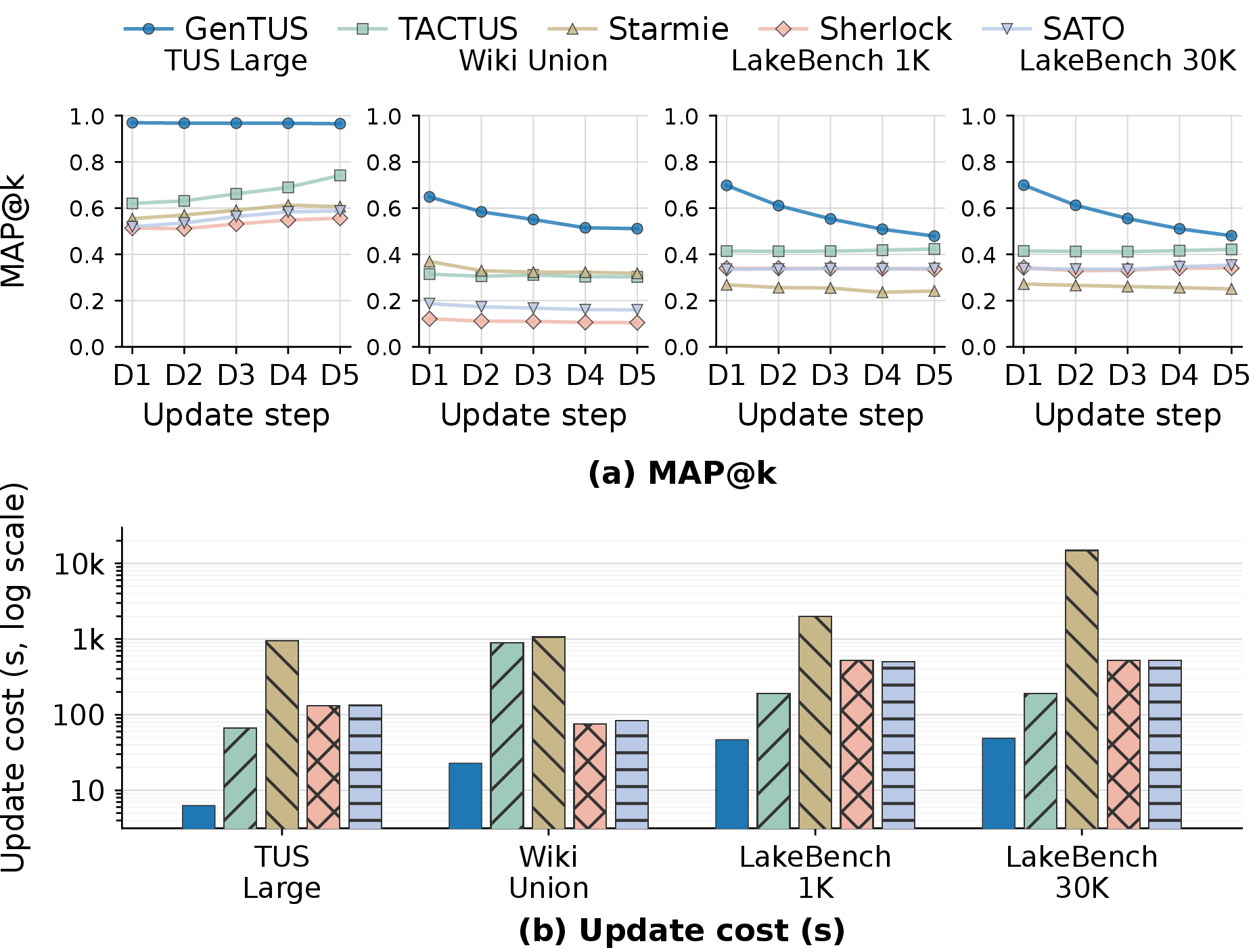
Effectiveness. Figure 11 (a) reports MAP over the update steps D1–D5. GenTUS attains the highest MAP on every dataset and at every step. At the final step D5 it reaches \(0.965\) on TUS_large against \(0.741\) for the next best method, \(0.511\) on wiki_union against \(0.318\), and about \(0.48\) on the two LakeBench splits against about \(0.42\). This shows that GenTUS with a frozen generator matches or outperforms baselines that encode and insert the newly added tables.
Update cost. Figure 11 (b) reports the time from updating the index to answering the first query. GenTUS is the fastest on every dataset, by one to two orders of magnitude over the baselines. Adding a table requires encoding the new table, residual quantization, and a single prefix-tree insertion, but does not re-encode existing tables or rebuild a dense index. For instance, on LakeBench_30k GenTUS answers in \(49\) seconds versus \(191\) seconds for TACTUS and about four hours for Starmie. Overall, GenTUS indexes new tables at substantially lower cost and consistently outperforms the incrementally updated baselines in retrieval quality.
7.5 Robustness to Candidate-Space Size↩︎
| Dataset | #Tables | GenTUS | TACTUS | Starmie | Sherlock | SATO |
|---|---|---|---|---|---|---|
| LB-1K | 1,000 | 0.627 | 0.426 | 0.270 | 0.394 | 0.405 |
| 2,500 | 0.634 | 0.432 | 0.291 | 0.411 | 0.412 | |
| 5,000 | 0.627 | 0.432 | 0.303 | 0.391 | 0.385 | |
| 7,970 | 0.602 | 0.429 | 0.304 | 0.368 | 0.364 | |
| LB-30K | 1,000 | 0.651 | 0.417 | 0.272 | 0.415 | 0.422 |
| 2,500 | 0.637 | 0.429 | 0.282 | 0.398 | 0.415 | |
| 5,000 | 0.632 | 0.427 | 0.299 | 0.388 | 0.399 | |
| 7,970 | 0.613 | 0.430 | 0.296 | 0.364 | 0.373 |
2pt
We next isolate the effect of candidate-space size on retrieval quality. Unlike the incremental-indexing experiment, this experiment follows the main full-data training setting and varies only the candidate pool used during evaluation. On the two LakeBench splits, we enlarge the pool from a small subset of \(1{,}000\) tables up to the full lake (Table 4). The largest pool is the full lake and matches the LakeBench setting in the main results (Table 2).
Robust across pool sizes. At every pool size, GenTUS attains the best MAP. As the candidate lake grows from \(1{,}000\) tables to the full lake, its MAP remains in a narrow range from \(0.602\) to \(0.651\). The baselines remain far behind at every pool size: about \(0.42\) to \(0.43\) for TACTUS, \(0.36\) to \(0.42\) for Sherlock and SATO, and \(0.27\) to \(0.30\) for Starmie. A smaller pool contains fewer distractor tables, while a larger pool adds many non-unionable tables that the truly unionable ones must be ranked above, which raises the pressure on top-\(k\) discrimination. Across this range, from a small pool to the full lake, GenTUS remains stable and preserves a clear margin over the strongest baseline.
7.6 Ablation and Analysis↩︎
The previous sections show that GenTUS works well as a whole. We now isolate how much each core design contributes, and how its main decoding hyperparameter behaves. We ablate two core designs, the construction of the semantic identifier and prefix-constrained decoding, and then analyze how beam width trades off accuracy against latency. These experiments explain where the effectiveness of GenTUS comes from, not just that it is effective.
| Variant | TUS-S | TUS-L | SAN-S | SAN-L | Wiki | LB-1K | LB-30K |
|---|---|---|---|---|---|---|---|
| Ordinary RQ | +0.266 | +0.031 | \(-0.002\) | +0.225 | +0.177 | +0.108 | +0.110 |
| Random | +0.518 | +0.911 | +0.424 | +0.486 | +0.073 | +0.237 | +0.243 |
| Atomic | +0.394 | +0.814 | +0.213 | +0.745 | +0.688 | +0.288 | +0.247 |
| No-Suffix | +0.118 | +0.167 | +0.058 | +0.238 | +0.246 | +0.299 | +0.342 |
3pt
Semantic identifier. We first ablate how the semantic identifier is constructed (Table 5). We report MAP gains over four variants: ordinary RQ without the unionability objective, random identifiers, atomic identifiers, and No-Suffix. Atomic identifiers use one unique token per table; No-Suffix drops collision suffixes and selects one table uniformly at random when a base identifier maps to multiple tables. The improvement over random and atomic identifiers remains substantial on most datasets, reaching \(+0.911\) over random identifiers and \(+0.814\) over atomic identifiers, confirming that the identifier should encode table semantics rather than be assigned arbitrarily. The improvement over No-Suffix is consistently positive across all datasets (\(+0.058\) to \(+0.342\)), showing that collision suffixes help keep tables uniquely addressable. The gain over ordinary RQ is more dataset-dependent: it is large on TUS_small, SANTOS_large and wiki_union (\(+0.266\), \(+0.225\) and \(+0.177\)), clear on two LakeBench splits, but small on TUS_large and essentially tied on SANTOS_small. This pattern does not reduce to a simple split between easy and difficult benchmarks; rather, it suggests that the extra unionability objective is a refinement whose benefit depends on how much ordinary RQ already captures the neighborhood structure of tables in a corpus. Overall, the ablation shows that semantic IDs should be both semantically meaningful and uniquely addressable, while the unionability-aware objective provides additional gains.
| Metric | TUS-S | TUS-L | SAN-S | SAN-L | Wiki | LB-1K | LB-30K |
|---|---|---|---|---|---|---|---|
| Inv. Rate | 0.005 | 0.004 | 0.128 | 0.604 | 0.242 | 0.379 | 0.395 |
| Added Rel./Q | 0.000 | 0.033 | 0.580 | 6.257 | 7.480 | 0.533 | 0.588 |
| \(\Delta\)MAP | 0.000 | 0.001 | 0.057 | 0.403 | 0.198 | 0.021 | 0.022 |
| \(\Delta\)Recall | 0.000 | 0.000 | 0.049 | 0.406 | 0.154 | 0.039 | 0.034 |
3pt
Prefix-constrained decoding. We next analyze prefix-constrained decoding (Table 6). The decoder uses a prefix tree over the table identifiers, so each decoding step only expands prefixes that can lead to an existing table. Unconstrained decoding can spend top-\(k\) outputs on invalid identifiers, whereas prefix constraints keep the output list within valid table candidates. Across all seven datasets, prefix constraints never reduce MAP or Recall. They have little effect on the two TUS datasets, where unconstrained decoding is already almost always valid. On SANTOS_large and wiki_union, however, constraints recover many relevant tables and raise MAP by \(0.403\) and \(0.198\), respectively. The two LakeBench splits also contain many invalid unconstrained outputs, but each query recovers fewer additional relevant tables; their MAP gains are therefore modest while still positive. Thus prefix-constrained decoding guarantees valid table identifiers and improves retrieval quality when those additional valid candidates include relevant tables.
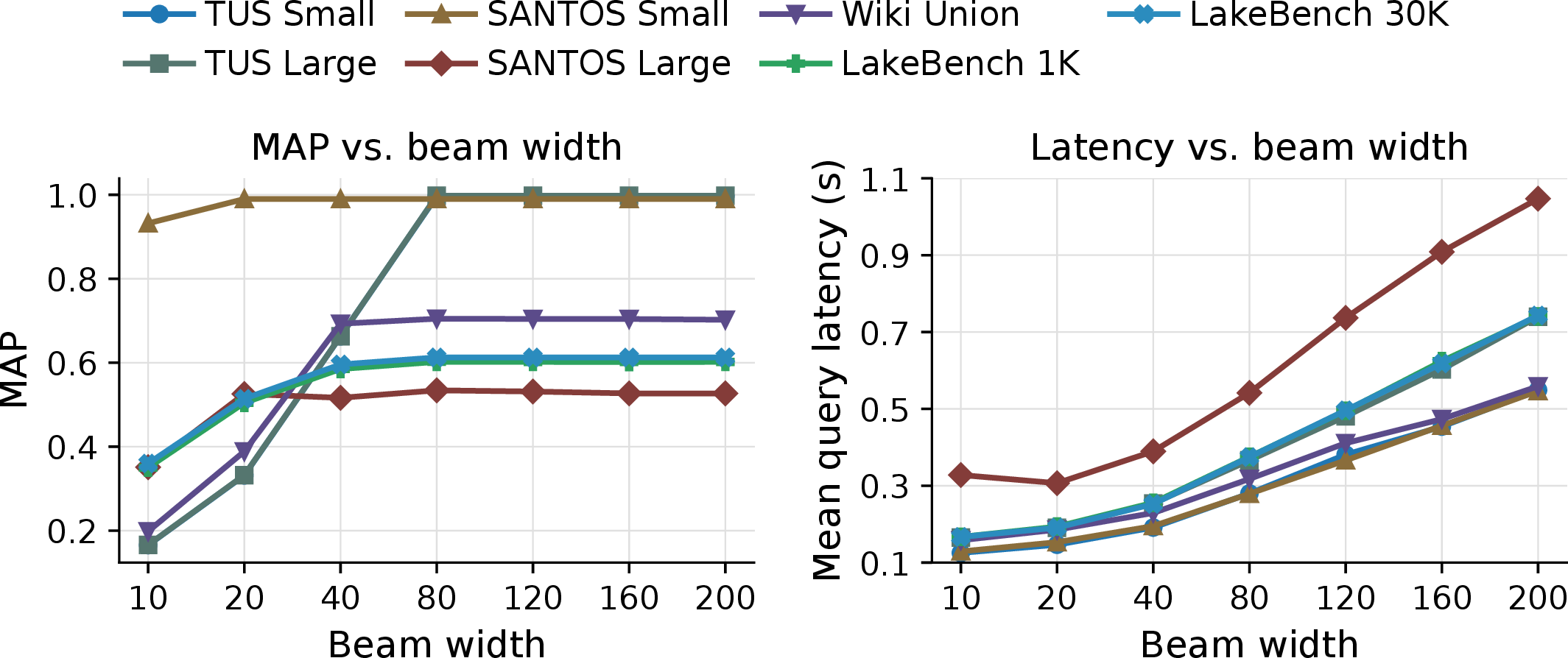
Beam width. Finally, we study how beam width trades off retrieval quality against online decoding cost (Figure 12), using the same checkpoints and query splits as the main effectiveness table. The quality curve rises sharply at small beams and then quickly saturates: SANTOS_large is already close to its best MAP by beam \(20\), while wiki_union and the two LakeBench splits reach their plateau around beam \(40\)–\(80\). Increasing the beam beyond this point brings little accuracy gain on the LakeBench splits, where MAP has already saturated. Latency generally increases with beam width because the decoder explores more identifier prefixes. Overall, the figure shows that a moderate beam is sufficient in practice: it recovers almost all of the attainable MAP while avoiding the much higher latency of the largest beams.
8 Conclusion↩︎
We presented GenTUS, a generative framework that reformulates table union search as constrained generation over discrete semantic table identifiers. Offline, GenTUS assigns each candidate table a residual-quantized identifier shaped by table-pair unionability annotations, and trains an encoder–decoder generator with a pairwise ranking objective. Online, a single prefix-constrained generation pass produces the top-\(k\) result, with no dense vector index and no per-candidate reranking. Across seven benchmarks, GenTUS improves retrieval quality while reducing offline build time, online retrieval time, and index storage. It also remains effective as the candidate pool grows and supports low-cost table insertion.
These results show that generative retrieval is a viable and practical alternative to encode–search–refine pipelines for TUS. Future work includes extending the formulation to joint unionable-table and joinable-table discovery, refreshing the identifier space and the generator incrementally under substantial distribution shift, and scaling the approach to even larger data lakes.
References↩︎
This work is licensed under the Creative Commons BY-NC-ND 4.0 International License. Visit https://creativecommons.org/licenses/by-nc-nd/4.0/ to view a copy of this license. For any use beyond those covered by this license, obtain permission by emailing info@vldb.org. Copyright is held by the owner/author(s). Publication rights licensed to the VLDB Endowment.
Proceedings of the VLDB Endowment, Vol. XX, No. XXISSN 2150-8097.
doi:XX.XX/XXX.XX
↩︎