Hybridizable Staggered Discontinuous Galerkin Methods for Polyharmonic Equations on Polytopes
July 01, 2026
Abstract
Hybridizable staggered discontinuous Galerkin methods are developed for arbitrary-order polyharmonic equations \((-\Delta)^m u=f\) on shape-regular polytopal meshes in \(\mathbb{R}^d\), for any \(m\ge1\), \(d\ge2\), and polynomial degree \(k\ge0\). The method uses the mixed variable \(\sigma=\nabla^m u\) and a staggered primal–dual mesh to impose complementary continuity on scalar and tensor unknowns, without restrictions such as \(d\ge m\). Local trace and bubble enrichments stabilize low-order tensor spaces without adding global unknowns. Hybridization localizes the tensor variable and yields an equivalent stabilization-free weak Galerkin formulation. Well-posedness and optimal energy error estimates are proved, and numerical experiments on polygonal and tetrahedral meshes confirm the predicted rates.
1 Introduction↩︎
Let \(\Omega\) be a bounded polyhedral domain in \(\mathbb{R}^d\), \(d\ge2\). In this paper, we develop hybridizable staggered discontinuous Galerkin (HSDG) methods for the \(2m\)-th order polyharmonic problem, for \(m\ge1\), \[\label{intro:polyharmonic} \begin{cases} (-1)^m\Delta^m u=f, & \textrm{in }\Omega,\\ u=\partial_n u=\cdots=\partial_n^{m-1}u=0, & \textrm{on }\partial\Omega. \end{cases}\tag{1}\] The method is designed for general polytopal meshes, arbitrary order \(m\geq 1\), arbitrary dimension \(d\geq 2\), and all polynomial degrees \(k\ge0\). Its main ingredients are a staggered primal–dual mesh, a mixed tensor formulation, local tensor enrichments for low-order spaces, and a hybridization procedure that reduces the global system to scalar and face unknowns.
The starting point is the mixed formulation \[\label{intro:mixfem} \sigma=\nabla^m u,\qquad (-1)^m\operatorname{div}^m\sigma=f .\tag{2}\] Formally, the relation \(\sigma=\nabla^m u\) can be written as \[(\sigma,\tau)=(-1)^m(\operatorname{div}^m\tau,u),\] so the scalar unknown only needs to be in \(L^2(\Omega)\), while the tensor unknown carries the \(H(\operatorname{div}^m)\)-type regularity. For \(m=1\), this is the classical mixed formulation based on \(H(\operatorname{div})\)-conforming spaces, including Raviart–Thomas, Brezzi–Douglas–Marini, Nédélec, and related elements [1]–[5]. For \(m=2\), several \(H(\operatorname{div}\operatorname{div})\)-conforming finite element spaces have recently been developed [6]–[10]. For general \(m\), constructing explicit \(H(\operatorname{div}^m)\)-conforming tensor finite elements is difficult, especially on general polytopes.
The staggered discontinuous Galerkin (SDG) framework provides a different way to impose the mixed regularity. SDG methods, initiated by Chung and Engquist [11], [12], use staggered primal and dual grids to obtain stable and locally conservative discretizations. They have been extended from triangular meshes to polygonal meshes in [13]–[15], and a primal SDG method on polytopal meshes was recently developed in [16]. The present work extends [16] from second-order problems to arbitrary-order polyharmonic equations.
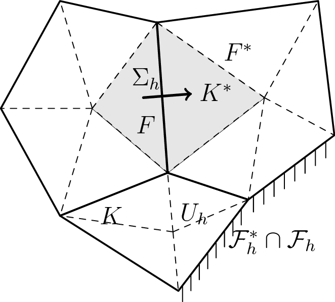
Given a polyhedral primal mesh \(\mathcal{K}_h\), each element \(K\) is split by connecting an interior point of \(K\) to its faces, giving a refined mesh \(\mathcal{K}_h^{\rm R}\). The dual mesh \(\mathcal{K}_h^*\) is formed by grouping refined cells that share a primal face. The key SDG idea is to impose complementary continuity on the primal and dual meshes. The tensor variable \(\sigma_h\) satisfies the required \(H(\operatorname{div}^m)\)-type conformity on dual elements, while the scalar variable \(u_h\) is locally \(H^m\)-conforming on primal elements. Thus both variables are globally discontinuous, but their continuity properties are staggered and complementary. This gives a stable mixed discretization of 2 without constructing globally \(H(\operatorname{div}^m)\)-conforming tensor elements on the primal polytopal mesh.
The scalar space is chosen elementwise as \(\mathbb{P}_{k+m}(K)\) on each primal element. The main difficulty is to construct tensor spaces \(\Sigma_{h,k}\) for an arbitrary number of face-normal directions, order \(m\), dimension \(d\), and polynomial degree \(k\). Two local enrichments are used. The trace enrichment recovers missing normal trace layers when \(k<m-1\). The bubble enrichment provides enough tensor directions for the local stability construction. If \(\nu_K\) is the largest number of pairwise non-parallel face normals of \(K\), then tensor layers up to order \(\lfloor m/\nu_K\rfloor\) are enough.
The method is naturally hybridizable. Following the hybridization framework for mixed methods [17], [18], we relax the primal-face continuity of the tensor traces, use a fully broken tensor space on the refined mesh, and introduce scalar trace unknowns on primal faces. The weak \(m\)-th gradient \(\nabla^m_w\) is defined so that the tensor unknown can be eliminated element by element. After static condensation, the global problem involves only the scalar variable and its face traces and is equivalent to a weak Galerkin formulation without penalty stabilization. Stability comes from the staggered mixed structure and the local tensor trace construction, which yield coercivity of the discrete weak gradient after hybridization.
We now place the proposed method in context. The primal formulation of 1 uses the bilinear form \((\nabla^m u,\nabla^m v)\) and therefore requires an \(H^m\)-conforming discrete space. On simplicial meshes, this leads to highly smooth finite elements, such as those in [19]–[23]. A geometric decomposition of the simplicial lattice was introduced in [24], [25] and used for explicit basis construction and implementation in [26]. These conforming finite element spaces are explicit, but they require high polynomial degree \(2^d (m-1)+1\).
On general polytopes, conforming virtual element methods provide a flexible alternative. The \(H^m\)-conforming virtual elements of arbitrary degree \(k\ge m\) on polytopal meshes were constructed in [27], generalizing earlier two- and three-dimensional constructions [28]–[30]. These methods work on arbitrary polytopes and arbitrary degree, but the local shape functions are virtual and a nontrivial stabilization term is needed.
Nonconforming methods reduce the smoothness requirement. On simplicial meshes, minimal \(H^m\)-nonconforming elements were constructed for \(m\le d\) [31], [32] and later extended to \(m=d+1\) [33]; arbitrary \(m\) and \(d\) can also be handled by interior penalty techniques [34]. The minimal nonconforming elements correspond to the lowest-order case \(k=0\) in our notation. A related minimal bubble-enriched construction was proposed in [35]. On general polytopes, \(H^m\)-nonconforming virtual elements of arbitrary degree were developed in [36], [37]. These VEMs, however, require nontrivial stabilization. The present paper follows a different route: the primary object is a staggered mixed DG method, and its stability is obtained from complementary primal–dual continuity and tensor trace liftings, not from a primal nonconforming space with a stabilization term.
After local tensor elimination, the hybridized SDG method can be interpreted as a weak Galerkin or VEM-like method without penalty stabilization. In this interpretation, the scalar unknown and its face traces determine a local weak \(m\)-th gradient. Unlike standard VEM projections on a single polytopal element, the projection here is enriched from a polynomial space on \(K\) to a piecewise polynomial space on the barycentric split \(K^{\rm R}\). This larger local projection space replaces penalty stabilization.
The analysis is carried out under standard shape-regularity assumptions on the polytopal mesh and on the associated refined subcells. The constants in the stability and error estimates are uniform with respect to the mesh size \(h\) and may depend only on the fixed polynomial degree, the order \(m\), the dimension \(d\), and the mesh regularity parameters. These assumptions are stated precisely in Section 4.1.
The remainder of this article is organized as follows. Section 2 introduces the notation, tensor calculus, and staggered mesh structure. Section 3 proves the tensor polynomial decompositions and local trace constructions. Section 4 constructs the SDG finite element spaces and proves the well-posedness of the mixed method. Section 5 develops the hybridized SDG formulation and proves the error estimates. Section 6 reports numerical experiments supporting the theoretical results.
2 Symmetric Tensors and Decompositions↩︎
In this section, we recall basic notation for tensor spaces, contractions, tensor differential operators, and symmetric tensors. We then use simplicial lattices to index bases of symmetric tensor spaces and to describe polynomial layers relative to a face. Finally, we derive a geometric \(t\)-\(n\) decomposition of symmetric tensors and a face-based spanning decomposition that will be used in the construction of the local tensor spaces.
2.1 Tensors↩︎
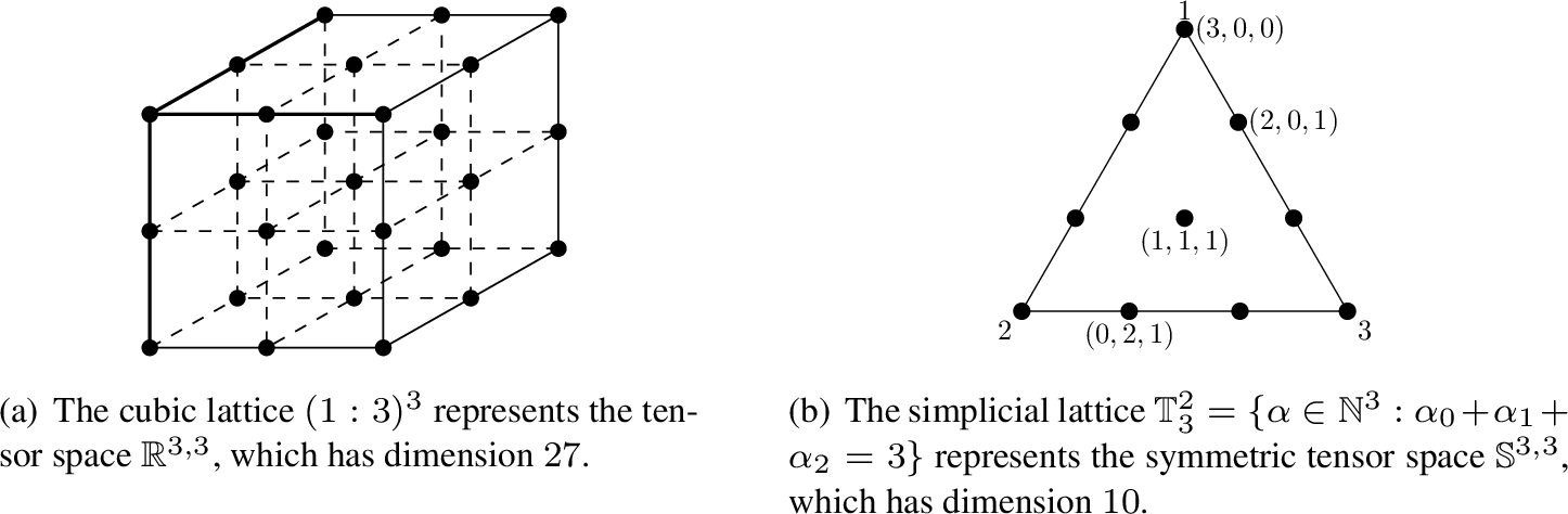
Denote the space of \(d\)-dimensional tensors of order \(m\) by \(\mathbb{R}^{d,m}:=(\mathbb{R}^d)^{\otimes m}.\) Let \(\{\boldsymbol{e}_1,\ldots,\boldsymbol{e}_d\}\) be an orthonormal basis of \(\mathbb{R}^d\). Then \[\left\{ \boldsymbol{e}_{i_1}\otimes\boldsymbol{e}_{i_2}\otimes\cdots\otimes\boldsymbol{e}_{i_m} : i_\ell\in\{1,\ldots,d\}, \;\ell=1,\ldots,m \right\}\] is a basis of \(\mathbb{R}^{d,m}\). Hence any \(\tau\in\mathbb{R}^{d,m}\) can be written as \[\tau = \tau_{i_1,\ldots,i_m} \boldsymbol{e}_{i_1}\otimes\boldsymbol{e}_{i_2}\otimes\cdots\otimes\boldsymbol{e}_{i_m},\] where repeated indices are summed over \(1,\ldots,d\). Therefore \(\dim\mathbb{R}^{d,m}=d^m.\) Equivalently, the basis can be represented by the integer lattice \(\{1,\ldots,d\}^m\); see Fig. 1 (a).
Let \(\tau\in\mathbb{R}^{d,m}\) and \(\gamma\in\mathbb{R}^{d,n}\) with \(0\le n\le m\). The contraction \[\tau\mathbin{\lrcorner}\gamma\in\mathbb{R}^{d,m-n}, \quad (\tau\mathbin{\lrcorner}\gamma)_{i_1,\ldots,i_{m-n}} := \tau_{i_1,\ldots,i_{m-n},j_1,\ldots,j_n} \gamma_{j_1,\ldots,j_n}.\] In particular, if \(n=1\), then \(\tau\mathbin{\lrcorner}\gamma\) is the tensor-vector contraction, extending the matrix-vector product. If \(n=m\), then \[\tau:\gamma := \tau\mathbin{\lrcorner}\gamma = \tau_{j_1,\ldots,j_m}\gamma_{j_1,\ldots,j_m}\] defines the Euclidean inner product on \(\mathbb{R}^{d,m}\), and the induced norm is the Frobenius norm.
For \(\tau\in\mathbb{R}^{d,m}\) and \(\boldsymbol{v}\in\mathbb{R}^d\), the outer product \(\tau\otimes\boldsymbol{v}\in\mathbb{R}^{d,m+1}\) is defined by \[(\tau\otimes\boldsymbol{v})_{i_1,\ldots,i_m,j} = \tau_{i_1,\ldots,i_m}v_j.\]
Let \(\Omega\subset\mathbb{R}^d\) be a domain. A tensor function on \(\Omega\) is a tensor whose coefficients are functions on \(\Omega\). For \(s\ge0\), define \(H^s(\Omega;\mathbb{R}^{d,m})\) as the space of tensor functions whose coefficients belong to \(H^s(\Omega)\). Let \(\mathbb{P}_k(T)\) be the space of polynomials of degree at most \(k\) on \(T\), with the convention \(\mathbb{P}_k(T)=\{0\}\) for \(k<0.\) For a finite-dimensional linear space \(V\), define \[\mathbb{P}_k(T;V):=\mathbb{P}_k(T)\otimes V.\] Equivalently, \(\mathbb{P}_k(T;V)\) is the space of \(V\)-valued polynomials of degree at most \(k\) on \(T\).
For \(\tau\in H^1(\Omega;\mathbb{R}^{d,m})\), the divergence is the tensor in \(L^2(\Omega;\mathbb{R}^{d,m-1})\) defined by \[(\operatorname{div}\tau)_{i_1,\ldots,i_{m-1}} = \partial_j\tau_{i_1,\ldots,i_{m-1},j}.\] For \(0\le s\le m\), let \(\operatorname{div}^s\) denote the operator obtained by applying divergence \(s\) times. With \(\nabla=(\partial_1,\ldots,\partial_d)^{\intercal}\), this can be written symbolically as \[\label{eq:tensor-div-symbolic} \operatorname{div}^{s}\tau = \tau\mathbin{\lrcorner}\nabla^s .\tag{3}\]
2.2 Symmetric tensors↩︎
Denote by \(\mathbb{S}^{d,m}\) the space of \(d\)-dimensional symmetric tensors of order \(m\). It is the subspace of \(\mathbb{R}^{d,m}\) consisting of tensors \(\tau\) such that \[\tau_{i_1,\ldots,i_m} = \tau_{i_{\sigma(1)},\ldots,i_{\sigma(m)}} \qquad \text{for all }\sigma\in\mathfrak S_m,\] where \(\mathfrak S_m\) is the symmetric group on \(\{1,\ldots,m\}\).
The symmetrization operator \(\operatorname{sym}:\mathbb{R}^{d,m}\to\mathbb{S}^{d,m}\) is defined by \[\operatorname{sym}(\boldsymbol{v}_1\otimes\cdots\otimes\boldsymbol{v}_m) = \frac{1}{m!} \sum_{\sigma\in\mathfrak S_m} \boldsymbol{v}_{\sigma(1)} \otimes\cdots\otimes \boldsymbol{v}_{\sigma(m)}, \qquad \boldsymbol{v}_1,\ldots,\boldsymbol{v}_m\in\mathbb{R}^d,\] and extended by linearity.
For \(v\in H^m(\Omega)\), define the \(m\)-th gradient by \[\nabla^m v := \nabla^{\otimes m}v = (\underbrace{\nabla\otimes\cdots\otimes\nabla}_{m})v, \quad (\nabla^m v)_{i_1,\ldots,i_m} = \partial_{i_1}\cdots\partial_{i_m}v.\] If \(v\) is sufficiently smooth, mixed partial derivatives commute. Hence \(\nabla^m v\in\mathbb{S}^{d,m}.\)
Let \(\alpha=(\alpha_1,\ldots,\alpha_d)\in\mathbb{N}^d\) be a multi-index, with \(|\alpha|=\sum_{i=1}^d\alpha_i\). For \(v\in C^m\), the \(m\)-th derivatives can also be indexed by \[D^\alpha v := \frac{\partial^m v}{\partial x_1^{\alpha_1}\cdots\partial x_d^{\alpha_d}}, \qquad |\alpha|=m.\] This multi-index notation gives a simplicial lattice representation of symmetric tensors.
2.3 Simplicial lattice representation↩︎
A simplicial lattice [24], [38] of degree \(r\) and dimension \(d\) is \[\mathbb{T}^{d}_r = \left\{ \alpha=(\alpha_0,\alpha_1,\ldots,\alpha_d)\in\mathbb{N}^{d+1} :\alpha_0+\alpha_1+\cdots+\alpha_d=r \right\}.\] Each \(\alpha\in\mathbb{T}^d_r\) is called a node of the lattice. Figure 1 (b) shows \(\mathbb{T}^2_3\).
For the symmetric tensor \(\operatorname{sym}(\boldsymbol{e}_{i_1}\otimes\cdots\otimes\boldsymbol{e}_{i_m})\), the order of the factors in \(\boldsymbol{e}_{i_1}\otimes\cdots\otimes\boldsymbol{e}_{i_m}\) is irrelevant up to permutation. Only the number of occurrences of each basis vector is relevant. Let \(\alpha_k\) be the number of factors equal to \(\boldsymbol{e}_k\) for \(k=1,\ldots,d\). Then \(\alpha=(\alpha_1,\ldots,\alpha_d)\) satisfies \(|\alpha|=m\). This set of multi-indices is identified with the lattice \(\mathbb{T}^{d-1}_m\). Therefore \[\left\{ \operatorname{sym}\!\left(\vcenter{\scalebox{1.5}{\otimes}}_{k=1}^d \boldsymbol{e}_k^{\alpha_k}\right) :\alpha\in\mathbb{T}^{d-1}_m \right\},\] where \(\boldsymbol{e}_k^{\alpha_k}:=\boldsymbol{e}_k^{\otimes\alpha_k}\), is a basis of \(\mathbb{S}^{d,m}\). Hence \[\dim\mathbb{S}^{d,m} = |\mathbb{T}^{d-1}_m| = \binom{m+d-1}{m},\] which is much smaller than \(\dim\mathbb{R}^{d,m}=d^m\).
2.4 Layer decomposition of the simplicial lattice↩︎
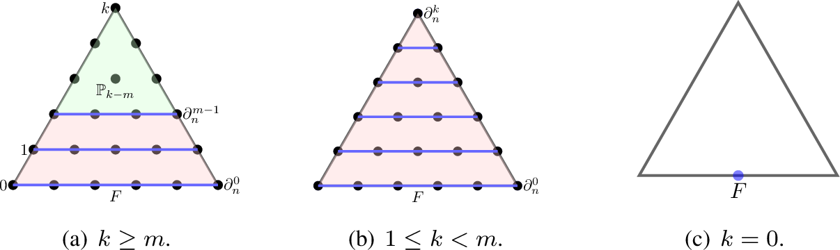
Let \(F\) be a face of a \(d\)-simplex \(T\). We label the barycentric coordinate opposite to \(F\) by index \(0\). Then each lattice point \(\alpha\in\mathbb{T}^d_k\) can be written as \[\alpha = (\alpha_0,\alpha_1,\ldots,\alpha_d) = \alpha_0\boldsymbol{e}_0+(0,\alpha_F),\] where \(\boldsymbol{e}_0=(1,0,\ldots,0)\) and \(\alpha_F=(\alpha_1,\ldots,\alpha_d)\in\mathbb{T}^{d-1}_{k-\alpha_0}.\) Define the distance of \(\alpha\) to \(F\) by \[\operatorname{dist}(\alpha,F):=\alpha_0, \qquad 0\le \alpha_0\le k.\] For \(0\le j\le k\), define the \(j\)-th layer by \[L_k^d(F,j) := \left\{ j\boldsymbol{e}_0+(0,\alpha_F): \alpha_F\in\mathbb{T}^{d-1}_{k-j} \right\}.\] Thus \(L_k^d(F,j)\) is the set of lattice points in \(\mathbb{T}^d_k\) at distance \(j\) from \(F\). The union of the layers \(L_k^d(F,j)\) for \(j=\ell,\ldots,k\) is a translated copy of the smaller lattice \(\mathbb{T}^d_{k-\ell}\); see Fig. 2 (a).
Lemma 1. The simplicial lattice admits the layer decomposition, for \(0\le \ell\le k\), \[\label{eq:latticedecomposition} \mathbb{T}^d_k = \bigsqcup_{j=0}^{k} L_k^d(F,j) = \bigsqcup_{j=0}^{\ell-1}L_k^d(F,j) \sqcup (\ell\boldsymbol{e}_0+\mathbb{T}^d_{k-\ell}).\qquad{(1)}\]
Proof. Each \(\alpha\in\mathbb{T}^d_k\) has a unique first component \(\alpha_0=j\), with \(0\le j\le k\). Hence \(\alpha\) belongs to exactly one layer \(L_k^d(F,j)\), which proves the first identity in ?? . The remaining points after removing the first \(\ell\) layers are precisely those with \(\alpha_0\ge\ell\). Writing \(\alpha=\ell\boldsymbol{e}_0+\beta\) gives \(\beta\in\mathbb{T}^d_{k-\ell}\), and this proves the second identity. ◻
2.5 Layer decomposition of polynomial spaces↩︎
Let \(T\) be a \(d\)-simplex with barycentric coordinates \(\{\lambda_i, i=0,\ldots, d\}\). We will apply the layer decomposition ?? to the Bernstein basis of \(\mathbb{P}_k(T)\), \[\mathbb{P}_k(T) = \operatorname{span}\{\lambda^\alpha:= \lambda_0^{\alpha_0}\lambda_1^{\alpha_1}\cdots\lambda_d^{\alpha_d} :\alpha\in\mathbb{T}^d_k\}.\] Since \(\lambda_0\) is the barycentric coordinate opposite to \(F\), the \(j\)-th lattice layer gives \[\operatorname{span}\{\lambda^\alpha:\alpha\in L_k^d(F,j)\} = \lambda_0^j\, \mathbb{P}_{k-j}(F).\]
Lemma 2. The polynomial space \(\mathbb{P}_k(T)\) has the layer decomposition, for \(0\le i\le k\), \[\label{eq:poly-layer-decomp} \mathbb{P}_k(T) = \vcenter{\scalebox{1.5}{\oplus}}_{j=0}^{k} \lambda_0^j\, \mathbb{P}_{k-j}(F) = \left( \vcenter{\scalebox{1.5}{\oplus}}_{j=0}^{i-1} \lambda_0^j\, \mathbb{P}_{k-j}(F) \right) \vcenter{\scalebox{1.5}{\oplus}} \lambda_0^i\, \mathbb{P}_{k-i}(T).\qquad{(2)}\]
Proof. The Bernstein basis functions are indexed by \(\mathbb{T}^d_k\). By ?? , each index \(\alpha\in\mathbb{T}^d_k\) belongs to exactly one layer \(L_k^d(F,j)\). If \(\alpha\in L_k^d(F,j)\), then \(\alpha_0=j\) and \[\lambda^\alpha = \lambda_0^j\lambda_F^{\alpha_F}, \qquad \alpha_F\in\mathbb{T}^{d-1}_{k-j}.\] Thus the functions from this layer span \(\lambda_0^j\, \mathbb{P}_{k-j}(F)\). Summing over \(j=0,\ldots,k\) gives the first identity ?? . The second identity follows by grouping all layers with \(j\ge i\): \[\vcenter{\scalebox{1.5}{\oplus}}_{j=i}^{k} \lambda_0^j\, \mathbb{P}_{k-j}(F) = \lambda_0^i \vcenter{\scalebox{1.5}{\oplus}}_{j=0}^{k-i} \lambda_0^{j}\, \mathbb{P}_{k-i-j}(F) = \lambda_0^i\, \mathbb{P}_{k-i}(T).\] The translated sublattice is illustrated in Fig. 2 (a). ◻
2.6 Layer decomposition of symmetric tensors↩︎
We use the layer decomposition of the lattice \(\mathbb{T}^{d-1}_m\) to decompose the symmetric tensor space \(\mathbb{S}^{d,m}\) with respect to a face \(F\).
Choose a local \(t\)-\(n\) coordinate system associated with \(F\), \[(\boldsymbol{t}_1,\ldots,\boldsymbol{t}_{d-1},\boldsymbol{n}_F),\] where \(\boldsymbol{t}_1,\ldots,\boldsymbol{t}_{d-1}\) form an orthonormal basis of the tangent space of \(F\) and \(\boldsymbol{n}_F\) is a unit normal vector.
For a tangential multi-index \(\alpha_F=(\alpha_1,\ldots,\alpha_{d-1})\), define \[\boldsymbol{t}^{\alpha_F} := \vcenter{\scalebox{1.5}{\otimes}}_{i=1}^{d-1}\boldsymbol{t}_i^{\alpha_i}.\] Using the \(t\)-\(n\) basis, the symmetric tensor space is spanned by \[\mathbb{S}^{d,m} = \operatorname{span} \left\{ \operatorname{sym}\big( \boldsymbol{n}_F^\ell\otimes\boldsymbol{t}^{\alpha_F} \big) : 0\le\ell\le m,\; \alpha_F\in\mathbb{T}^{d-2}_{m-\ell} \right\}.\] Define the \(\ell\)-th normal layer by \[\mathbb{S}^{(\ell)}_{F,m} := \operatorname{span} \left\{ \operatorname{sym}\big( \boldsymbol{n}_F^\ell\otimes\boldsymbol{t}^{\alpha_F} \big) : \alpha_F\in\mathbb{T}^{d-2}_{m-\ell} \right\}, \quad 0\le\ell\le m.\]
Lemma 3. The symmetric tensor space \(\mathbb{S}^{d,m}\) admits the orthogonal \(t\)-\(n\) decomposition \[\label{eq:Sdecomp0} \mathbb{S}^{d,m} = \vcenter{\scalebox{1.5}{\oplus}}_{\ell=0}^{m} \mathbb{S}^{(\ell)}_{F,m} = \left( \vcenter{\scalebox{1.5}{\oplus}}_{\ell=0}^{r-1} \mathbb{S}^{(\ell)}_{F,m} \right) \vcenter{\scalebox{1.5}{\oplus}} \operatorname{sym}\big( \boldsymbol{n}_F^r\otimes\mathbb{S}^{d,m-r} \big), \qquad 0\le r\le m .\qquad{(3)}\]
Proof. The set \(\{\boldsymbol{t}_1,\ldots,\boldsymbol{t}_{d-1},\boldsymbol{n}_F\}\) is an orthonormal basis of \(\mathbb{R}^d\). Hence the symmetrized tensor products formed from this basis span \(\mathbb{S}^{d,m}\). The subspace \(\mathbb{S}^{(\ell)}_{F,m}\) consists of tensors with exactly \(\ell\) normal factors. Terms with different numbers of normal factors are orthogonal under the Frobenius inner product. Thus the first identity follows.
For the second identity, we use \[\vcenter{\scalebox{1.5}{\oplus}}_{\ell=r}^{m} \mathbb{S}^{(\ell)}_{F,m} = \left\{ \operatorname{sym}(\boldsymbol{n}_F^r\otimes \eta): \eta\in \vcenter{\scalebox{1.5}{\oplus}}_{\ell=0}^{m-r} \mathbb{S}^{(\ell)}_{F,m-r} \right\} = \operatorname{sym}\big(\boldsymbol{n}_F^r\otimes \mathbb{S}^{d,m-r}\big).\] Indeed, after factoring out \(r\) normal vectors, by the first identity, \(\vcenter{\scalebox{1.5}{\oplus}}_{\ell=0}^{m-r} \mathbb{S}^{(\ell)}_{F,m-r} = \mathbb{S}^{d,m-r}\). Combining this with the first decomposition proves ?? . ◻
2.7 Geometric decomposition using all faces↩︎
Definition 1. For a polytopal element \(K\subset\mathbb{R}^d\), define \(\nu_K\) as the largest number of faces of \(K\) whose unit outward normal vectors are pairwise non-parallel. Equivalently, \(\nu_K\) is the largest integer such that there exist faces \(F_1,\ldots,F_{\nu_K}\subset\partial K\) with unit outward normal vectors \(\boldsymbol{n}_{F_1},\ldots,\boldsymbol{n}_{F_{\nu_K}}\) satisfying \[\boldsymbol{n}_{F_i} \neq c\boldsymbol{n}_{F_j}, \qquad i\neq j,\quad c\in\mathbb{R}\setminus\{0\}.\]
If \(K\) is a bounded full-dimensional polytope, then \[d \le \nu_K \le \#\{F:\;F\subset\partial K\}.\] Indeed, if the face normals had fewer than \(d\) pairwise non-parallel directions, then they would span a proper subspace of \(\mathbb{R}^d\). A nonzero vector orthogonal to this span would be tangent to all supporting hyperplanes of \(K\), contradicting the boundedness of \(K\). The upper bound follows from the definition. The lower bound \(\nu_K=d\) is achieved by parallelepipeds, while for a \(d\)-simplex one has \(\nu_K=d+1\).
For a fixed \(K\), write \(\nu:=\nu_K\). Then \[\nu(\left\lfloor\frac{m}{\nu}\right\rfloor+1)>m.\] This elementary inequality will be used in the proof below.
Lemma 4. Let \(K\) be a polytopal element, and let \(F_1,\ldots,F_\nu\subset\partial K\) be faces whose outward unit normal vectors \(\boldsymbol{n}_1,\ldots,\boldsymbol{n}_\nu\) are pairwise non-parallel. Then \[\label{simplexmeshcondition} \mathbb{S}^{d,m} = \sum_{i=1}^{\nu} \sum_{\ell=0}^{\left\lfloor\frac{m}{\nu}\right\rfloor} \mathbb{S}^{(\ell)}_{F_i,m}.\qquad{(4)}\]
Proof. Let \(\mathcal{W} := \sum_{i=1}^{\nu} \sum_{\ell=0}^{\left\lfloor\frac{m}{\nu}\right\rfloor} \mathbb{S}^{(\ell)}_{F_i,m}.\) It is enough to prove \(\mathcal{W}^\perp=\{0\}\).
Associate to each \(\tau\in\mathbb{S}^{d,m}\) the homogeneous polynomial \[p_\tau(x) := \tau:x^{\otimes m} = \tau_{i_1,\ldots,i_m}x_{i_1}\cdots x_{i_m}, \qquad x\in\mathbb{R}^d.\] This map is injective.
Suppose \(\tau\in\mathcal{W}^\perp\). Fix \(i\in\{1,\ldots,\nu\}\) and decompose \[x = x_F+x_n\boldsymbol{n}_i, \qquad x_F\perp \boldsymbol{n}_i, \quad x_n=x\cdot\boldsymbol{n}_i.\] Since \(\tau\) is orthogonal to \(\mathbb{S}^{(\ell)}_{F_i,m}\) for \(\ell=0,\ldots,\left\lfloor\frac{m}{\nu}\right\rfloor\), the polynomial \(p_\tau(x_F+x_n\boldsymbol{n}_i)\) has no terms \(x_n^0,\ldots,x_n^{\left\lfloor\frac{m}{\nu}\right\rfloor}\). Hence \[p_\tau(x_F+x_n\boldsymbol{n}_i) = x_n^{\left\lfloor\frac{m}{\nu}\right\rfloor+1}q_i(x_F,x_n),\] or equivalently, \[(x\cdot\boldsymbol{n}_i)^{\left\lfloor\frac{m}{\nu}\right\rfloor+1} \mid p_\tau(x).\] This holds for every \(i=1,\ldots,\nu\).
Since the linear forms \(x\cdot\boldsymbol{n}_i\), \(i=1,\ldots,\nu\), are pairwise non-proportional, they are pairwise coprime. Therefore \[\prod_{i=1}^{\nu} (x\cdot\boldsymbol{n}_i)^{\left\lfloor\frac{m}{\nu}\right\rfloor+1} \mid p_\tau(x).\] The degree of this divisor is \(\nu(\left\lfloor\frac{m}{\nu}\right\rfloor+1)>m\), whereas \(p_\tau\) has degree \(m\). Hence \(p_\tau\equiv0\). By injectivity of \(\tau\mapsto p_\tau\), we obtain \(\tau=0\). Thus \(\mathcal{W}^\perp=\{0\}\), and hence \(\mathcal{W}=\mathbb{S}^{d,m}\). ◻
Example 1 (Simplex and parallelepiped). Let \(K\) be a \(d\)-simplex. Then \(\nu=d+1\). If \(d\ge m\), then \(\lfloor m/(d+1)\rfloor=0\), and the tangential tensor spaces from all faces span \(\mathbb{S}^{d,m}\).
If \(d<m\), then higher normal layers are needed in general. For example, if \(d=2\) and \(m=5\), then \(\nu=3\). Hence \[\mathbb{S}^{2,5} = \sum_{F\subset\partial K} \left( \mathbb{S}^{(0)}_{F,5} + \mathbb{S}^{(1)}_{F,5} \right).\]
For a parallelepiped in \(\mathbb{R}^d\), opposite faces have parallel normals, so \(\nu=d\). Hence the same statement holds with \(d+1\) replaced by \(d\).
Example 2 (Polygon with many normal directions). Let \(K\) be a polygon in \(\mathbb{R}^2\) with \(N\) edges and no two edge normals parallel. Then \(\nu=N\). If \(N>m\), then \(\left\lfloor\frac{m}{N}\right\rfloor=0\). Thus, for a polygon with enough edge directions, the tangential layers alone span \(\mathbb{S}^{2,m}\).
3 Finite Elements for Symmetric Tensors↩︎
In this section, we construct local finite element spaces for symmetric tensor fields. We first introduce a scalar single-face finite element and its normal Taylor decomposition. We then combine this scalar decomposition with the \(t\)-\(n\) decomposition of symmetric tensors to describe normal trace spaces and bubble spaces. Finally, we assemble these single-face spaces on a polytopal element.
3.1 Single-face finite element↩︎
Let \(T\subset\mathbb{R}^d\) be a single-face cell with distinguished face \(F\) and vertex \(c\) opposite to \(F\). Let \(\lambda_c\) be the affine function satisfying \[\lambda_c(c)=1, \qquad \lambda_c|_F=0.\] Then \(\nabla\lambda_c\perp F\) and \[\nabla\lambda_c=(\partial_n\lambda_c)\boldsymbol{n}_F, \qquad \partial_n\lambda_c=\frac{1}{\operatorname{dist}(c,F)}.\]
Although \(T=\operatorname{conv}(c,F)\) need not be a simplex, we may use simplex coordinates as auxiliary affine coordinates. Choose a nondegenerate \((d-1)\)-simplex \(S_F\subset F\) and let \(\widehat T_F:=\operatorname{conv}(c,S_F).\) Let \(\lambda_c,\lambda_1,\ldots,\lambda_d\) be the barycentric coordinates of \(\widehat T_F\). These functions are affine on the whole space \(\mathbb{R}^d\). Therefore their restrictions to \(T\) may be used to represent polynomials on \(T\). In particular, \[\mathbb{P}_k(T) = \operatorname{span}\{\lambda^\alpha:\alpha\in\mathbb{T}^d_k\},\] where \[\lambda^\alpha = \lambda_c^{\alpha_0}\lambda_F^{\alpha_F}, \qquad \lambda_F^{\alpha_F} = \lambda_1^{\alpha_1}\cdots\lambda_d^{\alpha_d}.\] We identify a polynomial on \(F\) with its extension to \(T\) obtained by using the same monomials \(\lambda_F^{\alpha_F}\), now viewed as affine functions on \(T\). With this convention, for \(k\ge0\) and \(i\ge0\), the polynomial space has the normal-layer decomposition \[\label{eq:Pkgeodecomp1} \mathbb{P}_k(T) = \left( \vcenter{\scalebox{1.5}{\oplus}}_{j=0}^{i-1}\lambda_c^j\mathbb{P}_{k-j}(F) \right) \vcenter{\scalebox{1.5}{\oplus}} \lambda_c^i\mathbb{P}_{k-i}(T),\tag{4}\] with the convention \(\mathbb{P}_s=\{0\}\) if \(s<0\).
Lemma 5. Let \(T\) be a single-face cell with distinguished face \(F\). For integers \(k\ge0\) and \(m\geq 1\), the space \(\mathbb{P}_k(T)\) is uniquely determined by the following degrees of freedom: \[\label{eq:PkDoFs} \begin{align} \label{eq:PkDoFs1} \int_F \partial_n^i v\,q\,\mathrm dS, &\qquad q\in\mathbb{P}_{k-i}(F), \quad i=0,1,\ldots,m-1,\\ \label{eq:PkDoFs2} \int_T v\,q\,\mathrm dx, &\qquad q\in\mathbb{P}_{k-m}(T). \end{align}\] {#eq: sublabel=eq:eq:PkDoFs,eq:eq:PkDoFs1,eq:eq:PkDoFs2}
Proof. By 4 with \(i=m\), every \(p\in\mathbb{P}_k(T)\) can be written as \[p = \sum_{i=0}^{m-1}\lambda_c^i p_i + \lambda_c^m p_m,\] where \(p_i\in\mathbb{P}_{k-i}(F)\) for \(i=0,\ldots,m-1\), and \(p_m\in\mathbb{P}_{k-m}(T)\). Since \(\lambda_c|_F=0\) and \(\partial_n\lambda_c\ne0\) on \(F\), the vanishing of the face DoFs ?? implies successively that \[p_0=p_1=\cdots=p_{m-1}=0.\] Hence \(p=\lambda_c^m p_m\). Taking \(q=p_m\) in ?? gives \[0 = \int_T \lambda_c^m p_m^2\,\mathrm dx.\] Since \(\lambda_c\ge0\) on \(T\) and is positive in the interior of \(T\), we obtain \(p_m=0\). Thus \(p=0\). Since the number of DoFs equals \(\dim\mathbb{P}_k(T)\), the DoFs are unisolvent. ◻
Introduce the single-face trace operator \[\operatorname{tr}_F^{H^m}v = (v,\partial_n v,\ldots,\partial_n^{m-1}v)|_F.\] Then 4 gives \[\mathbb{B}_k^{H^m}(T) := \ker(\operatorname{tr}_F^{H^m})\cap\mathbb{P}_k(T) = \lambda_c^m\mathbb{P}_{k-m}(T).\] When \(k<m\), \(\mathbb{B}_k^{H^m}(T)=\{0\}\).
3.2 Polynomial symmetric tensors and normal traces↩︎
Combining the polynomial decomposition 4 with the \(t\)-\(n\) decomposition of \(\mathbb{S}^{d,m}\), we obtain \[\label{eq:PkSdecomp} \mathbb{P}_k(T;\mathbb{S}^{d,m}) = \vcenter{\scalebox{1.5}{\oplus}}_{i=0}^{k} \vcenter{\scalebox{1.5}{\oplus}}_{\ell=0}^{m} \lambda_c^i\mathbb{P}_{k-i}(F;\mathbb{S}^{(\ell)}_{F,m}).\tag{5}\] This decomposition is indexed by pairs \((i,\ell)\), where \(i\) is the polynomial layer in the normal direction and \(\ell\) is the number of normal tensor factors; see Fig. 3.
Define the normal trace component \[\gamma_s(\tau) := ((\operatorname{div}^s\tau)\mathbin{\lrcorner}\boldsymbol{n}_F)|_F, \qquad 0\le s\le m-1.\] The full normal trace is \[\operatorname{tr}_F^{\operatorname{div}^m}\tau := (\gamma_0(\tau),\gamma_1(\tau),\ldots,\gamma_{m-1}(\tau)).\] For \(\tau=a(x)\eta\) with a scalar function \(a\) and a constant tensor \(\eta\in\mathbb{R}^{d,m}\), we have \[(\operatorname{div}^s\tau)_{i_1\cdots i_{m-s}} = \partial_{j_1}\cdots\partial_{j_s} \big(a\,\eta_{i_1\cdots i_{m-s}j_1\cdots j_s}\big) = (\partial_{j_1}\cdots\partial_{j_s}a) \eta_{i_1\cdots i_{m-s}j_1\cdots j_s}.\] Therefore, \[\operatorname{div}^s(a\eta) = \eta\mathbin{\lrcorner}\nabla^s a.\]
Lemma 6. Let \(q_F\in\mathbb{P}_{k-i}(F)\) and \(\eta_\ell\in\mathbb{S}^{(\ell)}_{F,m}\). Then, for \(i=0,1,\ldots,m-1\), \[\label{eq:firstnormaltrace} \gamma_i(\lambda_c^i q_F\eta_\ell) = i!(\partial_n\lambda_c)^i q_F (\eta_\ell\mathbin{\lrcorner}\boldsymbol{n}_F^{i+1}).\qquad{(5)}\] Moreover, \(\gamma_s(\lambda_c^i q_F\eta_\ell)=0\) for \(0\le s<i\). Consequently, if \(i\ge\ell\), then \[\operatorname{tr}_F^{\operatorname{div}^m}(\lambda_c^i q_F\eta_\ell)=0.\] If \(i<\ell\), then \(\gamma_i\) is injective on \[\lambda_c^i\mathbb{P}_{k-i}(F;\mathbb{S}^{(\ell)}_{F,m}).\] In addition, with the convention \(\mathbb{P}_{k-i}(F)=\{0\}\) if \(k-i<0\), \[\label{eq:gammai-image} \gamma_i\left( \vcenter{\scalebox{1.5}{\oplus}}_{\ell=i+1}^{m} \lambda_c^i\mathbb{P}_{k-i}(F;\mathbb{S}^{(\ell)}_{F,m}) \right) = \gamma_i\big(\mathbb{P}_k(T;\mathbb{S}^{d,m})\big) = \mathbb{P}_{k-i}(F;\mathbb{S}^{d,m-i-1}).\qquad{(6)}\]
Proof. Figure 3 illustrates how the trace operator acts on the \((i,\ell)\) block. Set \(p=\lambda_c^i q_F\). Since \(\eta_\ell\) is constant, \[\operatorname{div}^s(p\eta_\ell) = \eta_\ell\mathbin{\lrcorner}\nabla^s p.\] Also \(\lambda_c|_F=0\) and \[\nabla\lambda_c=(\partial_n\lambda_c)\boldsymbol{n}_F \qquad \text{on }F.\] If \(s<i\), every term in \(\nabla^s(\lambda_c^i q_F)\) contains a positive power of \(\lambda_c\) and hence vanishes on \(F\). Thus \[\gamma_s(\lambda_c^i q_F\eta_\ell)=0, \qquad 0\le s<i.\]
For \(s=i\), the only term that survives on \(F\) is the term in which all \(i\) derivatives hit \(\lambda_c^i\). Hence \[\nabla^i(\lambda_c^i q_F)|_F = i!(\partial_n\lambda_c)^i q_F\boldsymbol{n}_F^i.\] Using \[\operatorname{div}^i(\lambda_c^i q_F\eta_\ell) = \eta_\ell\mathbin{\lrcorner}\nabla^i(\lambda_c^i q_F),\] we get \[(\operatorname{div}^i(\lambda_c^i q_F\eta_\ell))|_F = i!(\partial_n\lambda_c)^i q_F (\eta_\ell\mathbin{\lrcorner}\boldsymbol{n}_F^i).\] The trace \(\gamma_i\) adds one more contraction with \(\boldsymbol{n}_F\), which proves ?? .
If \(s>i\), every surviving term still contains the factor produced by differentiating \(\lambda_c^i\) in the normal direction. After the additional normal contraction in \(\gamma_s\), each such term contains the factor \[\eta_\ell\mathbin{\lrcorner}\boldsymbol{n}_F^{i+1}.\] If \(i\ge\ell\), this contraction is zero because \(\eta_\ell\) contains only \(\ell\) normal factors. Therefore all trace components vanish.
If \(i<\ell\), then contraction with \(\boldsymbol{n}_F^{i+1}\) maps \(\mathbb{S}^{(\ell)}_{F,m}\) injectively into \(\mathbb{S}^{(\ell-i-1)}_{F,m-i-1}\). Indeed, for a basis tensor \[\eta_\ell = \operatorname{sym}(\boldsymbol{n}_F^\ell\otimes\boldsymbol{t}^{\alpha_F}),\] one has \[\eta_\ell\mathbin{\lrcorner}\boldsymbol{n}_F^{i+1} = c_{\ell,i,m}\, \operatorname{sym}(\boldsymbol{n}_F^{\ell-i-1}\otimes\boldsymbol{t}^{\alpha_F}),\] where \(c_{\ell,i,m}\ne0\). Hence ?? implies the injectivity of \(\gamma_i\) on the stated block.
It remains to prove ?? . From ?? , \[\gamma_i\left( \vcenter{\scalebox{1.5}{\oplus}}_{\ell=i+1}^{m} \lambda_c^i\mathbb{P}_{k-i}(F;\mathbb{S}^{(\ell)}_{F,m}) \right) = \mathbb{P}_{k-i}(F)\otimes \left( \vcenter{\scalebox{1.5}{\oplus}}_{\ell=i+1}^{m} (\mathbb{S}^{(\ell)}_{F,m}\mathbin{\lrcorner}\boldsymbol{n}_F^{i+1}) \right).\] The contraction by \(\boldsymbol{n}_F^{i+1}\) maps \(\mathbb{S}^{(\ell)}_{F,m}\) onto \(\mathbb{S}^{(\ell-i-1)}_{F,m-i-1}\) for \(\ell=i+1,\ldots,m\). Therefore \[\vcenter{\scalebox{1.5}{\oplus}}_{\ell=i+1}^{m} (\mathbb{S}^{(\ell)}_{F,m}\mathbin{\lrcorner}\boldsymbol{n}_F^{i+1}) = \vcenter{\scalebox{1.5}{\oplus}}_{r=0}^{m-i-1}\mathbb{S}^{(r)}_{F,m-i-1} = \mathbb{S}^{d,m-i-1}.\] Thus the left-hand side of ?? equals \(\mathbb{P}_{k-i}(F;\mathbb{S}^{d,m-i-1})\).
Conversely, for any \(\tau\in\mathbb{P}_k(T;\mathbb{S}^{d,m})\), the trace \(\gamma_i(\tau)\) contains \(i\) derivatives and one normal contraction. Hence \[\gamma_i(\tau)\in\mathbb{P}_{k-i}(F;\mathbb{S}^{d,m-i-1}).\] This gives the reverse inclusion and proves ?? . ◻
Define \[\mathbb{B}_k^{\operatorname{div}^m}(T;\mathbb{S}^{d,m}) := \ker(\operatorname{tr}_F^{\operatorname{div}^m}) \cap \mathbb{P}_k(T;\mathbb{S}^{d,m}).\] Lemma 6 gives the following characterization of the polynomial trace and bubble spaces.
Proposition 1. For \(k\ge0\), the polynomial bubble space is \[\label{eq:BkSdecomp} \mathbb{B}_k^{\operatorname{div}^m}(T;\mathbb{S}^{d,m}) = \vcenter{\scalebox{1.5}{\oplus}}_{\ell=0}^{m} \lambda_c^\ell\mathbb{P}_{k-\ell}(T;\mathbb{S}^{(\ell)}_{F,m}).\qquad{(7)}\] Moreover, the full trace map satisfies \[\label{eq:traceimagepoly} \operatorname{tr}_F^{\operatorname{div}^m} \big(\mathbb{P}_k(T;\mathbb{S}^{d,m})\big) = \prod_{i=0}^{m-1} \mathbb{P}_{k-i}(F;\mathbb{S}^{d,m-i-1}).\qquad{(8)}\]
Figure 3 shows the \((i,\ell)\)-indexed block layout. The lower-triangular cells \(i\ge\ell\) form the bubble space, while the upper-triangular cells \(i<\ell\) are detected by the normal traces.

3.3 Single-face enriched tensor space↩︎
The natural local polynomial tensor space is \(\mathbb{P}_k(T;\mathbb{S}^{d,m})\). To obtain stability for all polynomial degrees, we enrich this space by trace and bubble components. The trace enrichment is needed only when \(k<m-1\), while the bubble enrichment depends on the geometry of \(K\).
3.3.1 Trace cells↩︎
When \(k\ge m-1\), the polynomial tensor space already contains all trace layers. When \(k<m-1\), the trace components \(\gamma_i\), \(k+1\le i\le m-1\), are missing because \(\operatorname{div}^i\sigma=0\) for \(\sigma\in\mathbb{P}_k(T;\mathbb{S}^{d,m})\); see the white cells in Fig. 3 (b).
We will add more trace cells row by row and define the full trace-cell space by \[\label{eq:full-trace-space} \operatorname{Tr}(\Sigma_k;T) := \vcenter{\scalebox{1.5}{\oplus}}_{i=0}^{m-1} \lambda_c^i \mathbb{P}_{(k-i)^+}(F)\otimes \operatorname{sym}\big(\boldsymbol{n}_F^{i+1}\otimes\mathbb{S}^{d,m-i-1}\big),\tag{6}\] where \((k-i)^+ = \max\{k-i,0\}\).
3.3.2 Bubble cells↩︎
To prove the inf-sup condition, the local tensor space must contain enough bubble tensors to recover all tensors in \(\mathbb{P}_k(K;\mathbb{S}^{d,m})\). This requirement depends on the geometry of \(K\) through the number \(\nu_K\) of pairwise non-parallel face normals.
For fixed \(K\), write \(\nu:=\nu_K\). If \(\lfloor m/\nu\rfloor>0\), we add extra bubble cells so that all tensor layers up to order \(\lfloor m/\nu\rfloor\) carry degree \(k\). Define \[\label{eq:full-bubble-space} \begin{align} \mathbb{B}(\Sigma_k;T) :={}& \underbrace{ \vcenter{\scalebox{1.5}{\oplus}}_{\ell=0}^{\lfloor m/\nu\rfloor} \lambda_c^{\ell}\mathbb{P}_k(T;\mathbb{S}^{(\ell)}_{F,m}) }_{\mathbb{B}_{\mathrm{ess}}(T)} \vcenter{\scalebox{1.5}{\oplus}} \underbrace{ \vcenter{\scalebox{1.5}{\oplus}}_{\ell=\lfloor m/\nu\rfloor+1}^{m} \lambda_c^{\ell}\mathbb{P}_{k-\ell}(T;\mathbb{S}^{(\ell)}_{F,m}) }_{\mathbb{B}_{\mathrm{rem}}(T)} . \end{align}\tag{7}\]
3.3.3 Stress space and unisolvence↩︎
We define the local single-face stress space by the trace–bubble decomposition \[\label{eq:decomposition-tr-bubble} \Sigma_k(T) := \operatorname{Tr}(\Sigma_k;T) \vcenter{\scalebox{1.5}{\oplus}} \mathbb{B}(\Sigma_k;T).\tag{8}\]
The decomposition 8 gives the following degrees of freedom.
Lemma 7. Let \(m\ge1\) and \(k\ge0\). The following DoFs are unisolvent for \(\Sigma_k(T)\): \[\label{sfTtensordof} \begin{align} \label{sfTtensordof1} \int_F \gamma_i(\sigma):\tau\,\mathrm dS, &\qquad \tau\in \mathbb{P}_{(k-i)^+}(F;\mathbb{S}^{d,m-i-1}), \quad i=0,\ldots,m-1,\\ \label{sfTtensordof2} \int_T \sigma:\tau\,\mathrm dx, &\qquad \tau\in \mathbb{B}(\Sigma_k;T). \end{align}\] {#eq: sublabel=eq:sfTtensordof,eq:sfTtensordof1,eq:sfTtensordof2}
Proof. Let \(\sigma\in\Sigma_k(T)\) and assume that all DoFs in ?? vanish. Write \[\sigma = \sigma_{\operatorname{tr}} + \sigma_{\operatorname b}, \qquad \sigma_{\operatorname{tr}}\in\operatorname{Tr}(\Sigma_k;T), \quad \sigma_{\operatorname b}\in\mathbb{B}(\Sigma_k;T).\] By the construction of \(\operatorname{Tr}(\Sigma_k;T)\) and Lemma 6, the face moments ?? determine the trace part. Since all face moments vanish, we have \(\sigma_{\operatorname{tr}}=0\). Hence \(\sigma=\sigma_{\operatorname b}\in\mathbb{B}(\Sigma_k;T)\). Taking \(\tau=\sigma\) in ?? gives \(\|\sigma\|_{0,T}^2=0.\) Therefore \(\sigma=0\). Since the number of DoFs equals \(\dim\Sigma_k(T)\), the DoFs are unisolvent. ◻
Remark 2. When \(m\) is moderate, one may avoid the minimal enriched tensor space and use the full polynomial tensor space \[\mathbb{P}_{\bar k}(T;\mathbb{S}^{d,m}),\qquad \bar k= \max\{k+\lfloor m/\nu_K\rfloor, m-1\},\quad T\in\mathcal{K}_h^{\rm R},\] which contains \(\operatorname{Tr}(\Sigma_k;T)\vcenter{\scalebox{1.5}{\oplus}}\mathbb{B}(\Sigma_k;T)\). The minimal construction is used in the analysis to identify the needed trace and bubble components, while the full polynomial space gives a simpler implementation.
3.4 Finite element for symmetric tensors on a polytope↩︎
We now fix one polytope \(K\) and construct the local tensor space on \(K\). Let \(K^{\rm R}:=\{T_i\}_{i=1}^{n_K}\) be the local refinement associated with the faces \(F_i\subset\partial K\). We assume throughout that such a point \(c_K\) exists and that each \(T_F\) is contained in \(K\). Define the broken local stress space by \[\label{eq:broken-local-stress-space} \Sigma^{-1}_{k}(K^{\rm R}) := \prod_{T\in K^{\rm R}}\Sigma_k(T) = \operatorname{Tr}(\Sigma_k;K) \vcenter{\scalebox{1.5}{\oplus}} \mathbb{B}_k(\Sigma_k;K),\tag{9}\] where \[\operatorname{Tr}(\Sigma_k;K) := \prod_{T_F\in K^{\rm R}}\operatorname{Tr}(\Sigma_k;T_F), \qquad \mathbb{B}_k(\Sigma_k;K) := \prod_{T\in K^{\rm R}}\mathbb{B}(\Sigma_k;T).\] For \(\tau\in\mathbb{B}_k(\Sigma_k;K)\), the exterior traces satisfy \[\gamma_i(\tau)|_{\partial K}=0,\qquad i=0,\ldots,m-1.\] The trace condition is imposed only on the exterior faces \(F_i\subset\partial K\), not on the internal faces of the local refinement.
By Lemma 7 on each refined cell \(T\), we obtain the following DoFs on \(K\).
Lemma 8. Let \(K\) be a fixed polytope and let \(k\ge0\). The following degrees of freedom are unisolvent for \(\Sigma^{-1}_{k}(K^{\rm R})\): \[\label{Ktensordof} \begin{align} \label{Ktensordof1} \int_F \gamma_i(\sigma):\tau\,\mathrm dS, &\quad \tau\in \mathbb{P}_{(k-i)^+}(F;\mathbb{S}^{d,m-i-1}), \;i=0,\ldots,m-1,\;F\subset\partial K,\\ \label{Ktensordof2} \int_K \sigma:\tau\,\mathrm dx, &\quad \tau\in \mathbb{B}_k(\Sigma_k;K). \end{align}\] {#eq: sublabel=eq:Ktensordof,eq:Ktensordof1,eq:Ktensordof2}
To prove the discrete inf-sup condition, we use an equivalent set of interior DoFs. Let \[N_m:=\dim\mathbb{S}^{d,m}=\binom{m+d-1}{m}.\] By Lemma 4, we can choose faces \(F_\alpha\subset\partial K\), integers \(0\le r_\alpha\le \lfloor m/\nu\rfloor\), and tensors \[\{\xi_\alpha\in\mathbb{S}^{(r_\alpha)}_{F_\alpha,m}, \, \alpha=1,\ldots,N_m,\} \text{ is a basis of } \mathbb{S}^{d,m}.\] Let \(T_\alpha=T_{F_\alpha}\) and \(\lambda_\alpha\) be the affine function on \(T_\alpha\) satisfying \(\lambda_\alpha|_{F_\alpha}=0\) and \(\lambda_\alpha(c_K)=1\).
Define the essential bubble space on \(K\) as \[\label{eq:essential-bubble-space} \mathbb{B}_{\rm ess}(\Sigma_k;K) := \vcenter{\scalebox{1.5}{\oplus}}_{\alpha=1}^{N_m} \left\{ \lambda_\alpha^{r_\alpha} q_\alpha \xi_\alpha\,\chi_{T_\alpha}: q_\alpha\in\mathbb{P}_k(T_\alpha) \right\} \subset \mathbb{B}_k(\Sigma_k;K),\tag{10}\] where \(\chi_{T_\alpha}\) is the characteristic function of \(T_\alpha\). Let \(\mathbb{B}_{\rm rem}(\Sigma_k;K)\) be the \(L^2(K)\)-orthogonal complement of \(\mathbb{B}_{\rm ess}(\Sigma_k;K)\) in \(\mathbb{B}_k(\Sigma_k;K)\). Then \[\label{eq:bubble-essential-rem-split} \mathbb{B}_k(\Sigma_k;K) = \mathbb{B}_{\rm rem}(\Sigma_k;K) \vcenter{\scalebox{1.5}{\oplus}}^{\bot_{L^2(K)}} \mathbb{B}_{\rm ess}(\Sigma_k;K).\tag{11}\] We will change the DoF corresponding to \(\mathbb{B}_{\rm rem}(\Sigma_k;K)\) to \(\mathbb{P}_k(K;\mathbb{S}^{d,m})\).
Lemma 9. Let \(K\in\mathcal{K}_h\) and \(k\ge0\). The space \(\Sigma_k^{-1}(K^{\rm R})\) is uniquely determined by the following degrees of freedom: \[\label{Ksymtensordof} \begin{align} \label{Ksymtensordof1} \int_F \gamma_i(\sigma):\tau\,\mathrm dS, &\quad \tau\in \mathbb{P}_{(k-i)^+}(F;\mathbb{S}^{d,m-i-1}), \;i=0,\ldots,m-1,\;F\subset\partial K,\\ \label{Ksymtensordof2} \int_K \sigma:\tau\,\mathrm dx, &\quad \tau\in \mathbb{B}_{\rm rem}(\Sigma_k;K),\\ \label{Ksymtensordof3} \int_K \sigma:\tau\,\mathrm dx, &\quad \tau\in \mathbb{P}_k(K;\mathbb{S}^{d,m}). \end{align}\] {#eq: sublabel=eq:Ksymtensordof,eq:Ksymtensordof1,eq:Ksymtensordof2,eq:Ksymtensordof3}
Proof. By Lemma 8, it is enough to prove that the moments in ?? –?? are equivalent to the bubble moments in ?? . Let \(\sigma\in\mathbb{B}_k(\Sigma_k;K)\) and assume that all degrees of freedom ?? –?? vanish. By 11 , write \[\sigma=\sigma_{\rm rem}+\sigma_{\rm ess}, \qquad \sigma_{\rm rem}\in\mathbb{B}_{\rm rem}(\Sigma_k;K), \quad \sigma_{\rm ess}\in\mathbb{B}_{\rm ess}(\Sigma_k;K).\] Due to the \(L^2(K)\)-orthogonality, taking \(\tau=\sigma_{\rm rem}\) in ?? gives \[0=(\sigma,\sigma_{\rm rem})_K=\|\sigma_{\rm rem}\|_{0,K}^2,\] so \(\sigma_{\rm rem}=0\). Hence \[\label{eq:sigma-ess-expansion} \sigma=\sigma_{\rm ess} = \sum_{\alpha=1}^{N_m} \lambda_\alpha^{r_\alpha} q_\alpha\xi_\alpha\,\chi_{T_\alpha}, \qquad q_\alpha\in\mathbb{P}_k(T_\alpha).\tag{12}\] Let \(\{\widehat\xi_\alpha\}_{\alpha=1}^{N_m}\) be the Frobenius-dual basis of \(\{\xi_\alpha\}_{\alpha=1}^{N_m}\), so that \(\xi_\alpha:\widehat\xi_\beta=\delta_{\alpha\beta}\). Extend each \(q_\alpha\) to a polynomial in \(\mathbb{P}_k(K)\), still denoted by \(q_\alpha\). Taking \(\tau=q_\alpha\widehat\xi_\alpha\) in ?? gives \[0 = (\sigma,q_\alpha\widehat\xi_\alpha)_K = \int_{T_\alpha} \lambda_\alpha^{r_\alpha}q_\alpha^2\,\mathrm dx .\] Since \(\lambda_\alpha^{r_\alpha}\ge0\) on \(T_\alpha\) and is positive in its interior, \(q_\alpha=0\). Thus \(\sigma=0\). The number of degrees of freedom is unchanged by the splitting 11 and \(\dim\mathbb{B}_{\rm ess}(\Sigma_k;K)=\dim\mathbb{P}_k(K;\mathbb{S}^{d,m})\). Hence the degrees of freedom are unisolvent. ◻
4 Staggered Discontinuous Galerkin Methods↩︎
In this section, we define the staggered discontinuous Galerkin method for the polyharmonic problem. The tensor variable is normal-trace continuous across primal faces, while the scalar variable is locally \(H^m\) on each primal element.
4.1 Primal and dual meshes↩︎
Let \(\mathcal{K}_h\) be a shape-regular polytopal partition of \(\Omega\subset\mathbb{R}^d\). Let \(\mathcal{F}_h\) be the set of faces, \(\mathcal{F}_h^\partial\) the set of boundary faces, and \(\mathring{\mathcal{F}}_h:=\mathcal{F}_h\setminus\mathcal{F}_h^\partial\) the set of interior faces. We call \(\mathcal{K}_h\) the primal mesh.
For each \(K\in\mathcal{K}_h\), choose a point \(c_K\in K\). For each face \(F\subset\partial K\), define \[T_F:=\operatorname{conv}(c_K,F), \qquad K^{\rm R}:=\{T_F:\;F\subset\partial K\}.\] The collection of all such cells gives a refinement \(\mathcal{K}_h^{\rm R}\) of \(\mathcal{K}_h\). We assume that the points \(c_K\) are chosen so that \(\mathcal{K}_h^{\rm R}\) is uniformly shape regular, and that the number of faces of each element is uniformly bounded.
Let \(\mathcal{F}_h^{\rm R}\) be the set of faces of the refined mesh \(\mathcal{K}_h^{\rm R}\) and define \(\mathring{\mathcal{F}}_h^* := \mathcal{F}_h^{\rm R}\setminus\mathcal{F}_h.\) The faces in \(\mathring{\mathcal{F}}_h^*\) are the dual faces; they lie inside primal elements. For each primal face \(F\in\mathcal{F}_h\), let \(\omega_F\) be the union of refined cells in \(\mathcal{K}_h^{\rm R}\) that contain \(F\). The dual mesh is \[\mathcal{K}_h^* := \{\omega_F:\;F\in\mathcal{F}_h\}.\]
For each face \(F\), fix a unit normal \(\boldsymbol{n}_F\). When no confusion can arise, we write \(\boldsymbol{n}\) for the relevant unit normal. For an interior face \(F\), the jump \([\cdot]\) is taken with respect to \(\boldsymbol{n}_F\). On a boundary face, we use the convention \([w]=w\).
4.2 Broken spaces and weak operators↩︎
Define the broken scalar space \[H^m(\mathcal{K}_h) := \{v\in L^2(\Omega):\;v|_K\in H^m(K)\quad\text{for all }K\in\mathcal{K}_h\}.\] For the tensor variable, define \[H(\operatorname{div}^m,\mathcal{K}_h^*;\mathbb{S}^{d,m}) := \left\{ \tau\in L^2(\Omega;\mathbb{S}^{d,m}): \tau|_{K^*}\in H(\operatorname{div}^m,K^*;\mathbb{S}^{d,m}) \;\text{for all }K^*\in\mathcal{K}_h^* \right\}.\] Equivalently, \[H(\operatorname{div}^m,\mathcal{K}_h^*;\mathbb{S}^{d,m}) = \left\{ \tau\in H^m(\mathcal{K}_h^{\rm R};\mathbb{S}^{d,m}): [\operatorname{tr}_F^{\operatorname{div}^m}\tau]=0 \quad\text{for all }F\in\mathring{\mathcal{F}}_h \right\},\] where \[\operatorname{tr}_F^{\operatorname{div}^m}\tau = (\gamma_0(\tau),\gamma_1(\tau),\ldots,\gamma_{m-1}(\tau)), \; \gamma_i(\tau) = ((\operatorname{div}^i\tau)\mathbin{\lrcorner}\boldsymbol{n}_F)|_F, \; i = 0, \ldots, m-1.\] Thus the normal trace components are single-valued across primal faces. The tensor variable may jump across dual faces, while the scalar variable may jump across primal faces.
For \(u\in H^m(\mathcal{K}_h)\), define the weak gradient by \[\label{eq:weakgrad} \begin{align} \langle \nabla_w^m u,\tau\rangle :=\;& \sum_{K\in\mathcal{K}_h} (\nabla^m u,\tau)_K\\ &+ \sum_{j=0}^{m-1} (-1)^{m-j} \sum_{F\in\mathcal{F}_h} \left( [\nabla^j u], (\operatorname{div}^{m-1-j}\tau)\mathbin{\lrcorner}\boldsymbol{n} \right)_F, \end{align}\tag{13}\] for all \(\tau\in H(\operatorname{div}^m,\mathcal{K}_h^*;\mathbb{S}^{d,m})\). The jump terms in 13 appear only on primal faces, because \(u\) is single-valued and \(H^m\) inside each primal element.
For \(\sigma\in H(\operatorname{div}^m,\mathcal{K}_h^*;\mathbb{S}^{d,m})\), define the weak divergence by \[\label{eq:weakdiv} \begin{align} \langle \operatorname{div}_w^m\sigma,v\rangle :=\;& \sum_{K^*\in\mathcal{K}_h^*} (\operatorname{div}^m\sigma,v)_{K^*}\\ &+ \sum_{i=0}^{m-1} (-1)^{m-i} \sum_{F^*\in\mathring{\mathcal{F}}_h^*} \left( [(\operatorname{div}^{i}\sigma)\mathbin{\lrcorner}\boldsymbol{n}], \nabla^{m-i-1}v \right)_{F^*}, \end{align}\tag{14}\] for all \(v\in H^m(\mathcal{K}_h)\). The jump terms in 14 appear only on dual faces, because the corresponding normal traces of \(\sigma\) are single-valued on primal faces.
Lemma 10 (Adjointness). For all \(\sigma\in H(\operatorname{div}^m,\mathcal{K}_h^*;\mathbb{S}^{d,m})\) and all \(v\in H^m(\mathcal{K}_h)\), \[\label{eq:weak-adjointness} \langle \operatorname{div}_w^m\sigma,v\rangle = (-1)^m \langle \sigma, \nabla_w^m v\rangle .\qquad{(9)}\]
Proof. Integrating by parts \(m\) times on each refined cell \(T\in\mathcal{K}_h^{\rm R}\) gives volume terms together with face terms. On primal faces, the normal trace components \[(\operatorname{div}^{i}\sigma)\mathbin{\lrcorner}\boldsymbol{n}, \qquad i=0,\ldots,m-1,\] are single-valued by the definition of \(H(\operatorname{div}^m,\mathcal{K}_h^*;\mathbb{S}^{d,m})\). On dual faces, the traces of \(\nabla^{m-i-1}v\) are single-valued because \(v\in H^m(K)\) on each primal element. Collecting the remaining primal- and dual-face terms gives exactly 14 and 13 , and hence ?? . ◻
For \(k\ge0\), define the scalar space \[U_{h,k+m} := \{u_h\in L^2(\Omega):\;u_h|_K\in\mathbb{P}_{k+m}(K) \quad\text{for all }K\in\mathcal{K}_h\}.\] Let \(\Sigma_k(T)\) be the local tensor space 8 on each refined cell \(T\in K^{\rm R}\). Define \[\Sigma_k^{-1}(K^{\rm R}) := \prod_{T\in K^{\rm R}}\Sigma_k(T).\] The global tensor space is \[\begin{align} \Sigma_{h,k} := \big\{ \sigma_h\in L^2(\Omega;\mathbb{S}^{d,m}): &\;\sigma_h|_K\in\Sigma_k^{-1}(K^{\rm R}) \quad\text{for all }K\in\mathcal{K}_h, \notag\\ &\;\text{the trace DoFs in \eqref{Ktensordof1} are single-valued across every } F\in\mathring{\mathcal{F}}_h \big\}. \label{eq:global-stress-space} \end{align}\tag{15}\] Then \[\Sigma_{h,k} \subset H(\operatorname{div}^m,\mathcal{K}_h^*;\mathbb{S}^{d,m}).\]
4.3 The Staggered Discontinuous Galerkin method↩︎
For \(\sigma_h,\tau_h\in\Sigma_{h,k}\) and \(v_h\in U_{h,k+m}\), define \[\begin{align} a(\sigma_h,\tau_h) &:= (\sigma_h,\tau_h), \\ b_h(\sigma_h,v_h) &:= (-1)^{m-1} \langle \operatorname{div}_w^m\sigma_h,v_h\rangle = -\langle \nabla_w^m v_h,\sigma_h\rangle. \end{align}\] Equivalently, by 13 , \[\label{eq:bh-expanded} \begin{align} b_h(\sigma_h,v_h) ={}& -\sum_{K\in\mathcal{K}_h} (\sigma_h,\nabla^m v_h)_K \\ &+ \sum_{i=0}^{m-1} (-1)^i \sum_{F\in\mathcal{F}_h} \left( (\operatorname{div}^i\sigma_h)\mathbin{\lrcorner}\boldsymbol{n}, [\nabla^{m-i-1}v_h] \right)_F . \end{align}\tag{16}\]
We reindex \(i\) by \(j\) with relation \[\label{eq:kj-def} j=m-i-1, k_j:=\max\{k-(m-1-j),0\}=(k-i)^+.\tag{17}\] This index \(k_j\) is the effective polynomial degree of the stress trace paired with \([\nabla^j v_h]\) in 16 . Indeed, with \(j=m-i-1\), the jump \([\nabla^j v_h]\) is paired with \[\gamma_{m-1-j}(\sigma_h) = (\operatorname{div}^{m-1-j}\sigma_h)\mathbin{\lrcorner}\boldsymbol{n},\] whose degree is at most \(k_j\). Hence only the projected jump \(Q_{F,k_j}[\nabla^j v_h]\) is seen by \(b_h(\cdot,\cdot)\). Here \(Q_{F,r}\) is the \(L^2(F)\) projection onto \(\mathbb{P}_r(F)\), applied componentwise.
For \(v\in H^m(\mathcal{K}_h)\), define \[\label{eq:U-norm} \|v\|_{m,h}^2 := |v|_{H^m(\mathcal{K}_h)}^2 + \sum_{j=0}^{m-1} \sum_{F\in\mathcal{F}_h} h_F^{2j-2m+1} \left\| Q_{F,k_j} [\nabla^j v] \right\|_F^2.\tag{18}\] By the Poincaré inequality for broken \(H^1\) spaces in [39], \[\label{eq:hybrid-poincare} \|v\|_{H^{m-1}(\mathcal{K}_h)} \lesssim \|v\|_{m,h} \qquad \forall~v\in H^m(\mathcal{K}_h).\tag{19}\] Thus \(\|\cdot\|_{m,h}\) is a norm on \(H^m(\mathcal{K}_h)\).
For \(\tau_h\in\Sigma_{h,k}\), define \[\label{eq:Sigma-norm} \|\tau_h\|_{0,h}^2 := \|\tau_h\|^2 + \sum_{i=0}^{m-1} \sum_{F\in\mathcal{F}_h} h_F^{2i+1} \left\| (\operatorname{div}^i\tau_h)\mathbin{\lrcorner}\boldsymbol{n} \right\|_F^2.\tag{20}\] By inverse trace inequalities on the finite-dimensional local tensor spaces, \[\label{eq:sigmaJ-equivalence} \|\tau_h\|_{0,h} \eqsim \|\tau_h\| \qquad \forall~\tau_h\in\Sigma_{h,k}.\tag{21}\]
The SDG method is: find \((\sigma_h,u_h)\in\Sigma_{h,k}\times U_{h,k+m}\) such that \[\label{SDG} \begin{cases} a(\sigma_h,\tau_h)+b_h(\tau_h,u_h)=0, & \quad \forall~\tau_h\in\Sigma_{h,k},\\ b_h(\sigma_h,v_h)=-(f,v_h), & \quad \forall~v_h\in U_{h,k+m}. \end{cases}\tag{22}\]
By 21 , \(a(\cdot,\cdot)\) is coercive on \(\Sigma_{h,k}\) with respect to \(\|\cdot\|_{0, h}\): \[\label{eq:acoercive} a(\tau_h,\tau_h) = \|\tau_h\|^2 \gtrsim \|\tau_h\|_{0, h}^2.\tag{23}\] Moreover, based on 16 , using the Cauchy-Schwarz inequality with correct scaling, we have \[\label{eq:bcontinuity} |b_h(\sigma_h,v)| \lesssim \|\sigma_h\|_{0, h}\|v\|_{m, h} \qquad \forall~\sigma_h\in\Sigma_{h,k},\quad v\in H^m(\mathcal{K}_h).\tag{24}\]
The key is to verify the following inf-sup condition.
Lemma 11 (Discrete inf-sup condition). There exists a constant \(\beta>0\), independent of \(h\), such that \[\label{discreteinfsup} \inf_{u_h\in U_{h,k+m}} \sup_{0\ne \sigma_h\in\Sigma_{h,k}} \frac{b_h(\sigma_h,u_h)}{\|\sigma_h\|_{0, h}\|u_h\|_{m, h}} \ge \beta .\qquad{(10)}\]
Proof. Let \(u_h\in U_{h,k+m}\) be fixed. Since \(u_h|_K\in\mathbb{P}_{k+m}(K)\), we have \(\nabla^m u_h|_K\in \mathbb{P}_k(K;\mathbb{S}^{d,m}).\) We define \(\sigma_h\in\Sigma_{h,k}\) by the degrees of freedom in Lemma 9.
First, for each \(K\in\mathcal{K}_h\), prescribe the polynomial moment DoFs by \[\label{eq:infsup-volume-dof} (\sigma_h,\tau)_K = -(\nabla^m u_h,\tau)_K \qquad \forall~\tau\in\mathbb{P}_k(K;\mathbb{S}^{d,m}).\tag{25}\] Second, on each face \(F\in\mathcal{F}_h\) and for \(i=0,\ldots,m-1\), prescribe the trace DoFs by \[\label{eq:infsup-face-dof} (\operatorname{div}^i\sigma_h)\mathbin{\lrcorner}\boldsymbol{n} = (-1)^i h_F^{-2i-1} Q_{F,(k-i)^+} [\nabla^{m-i-1}u_h] \qquad\text{on }F,\tag{26}\] in the sense of the face moments ?? . On an interior face, the jump is taken with respect to the fixed normal \(\boldsymbol{n}_F\), so the prescribed trace is single-valued. Finally, set all remaining bubble DoFs in \(\mathbb{B}_{\rm rem}(\Sigma_k;K)\) to zero. By Lemma 9, these data determine a unique \(\sigma_h\in\Sigma_{h,k}\).
Using 16 , 25 , and 26 , we obtain \[\begin{align} b_h(\sigma_h,u_h) &= |u_h|_{H^m(\mathcal{K}_h)}^2 + \sum_{i=0}^{m-1} \sum_{F\in\mathcal{F}_h} h_F^{-2i-1} \left\| Q_{F,(k-i)^+} [\nabla^{m-i-1}u_h] \right\|_F^2 . \end{align}\] Re-indexing the jump terms by \(j=m-i-1\) and using \((k-i)^+ = k_j\) gives \[b_h(\sigma_h,u_h) = \|u_h\|_{m, h}^2 .\]
It remains to bound \(\sigma_h\). By the scaling of the degrees of freedom in Lemma 9, the prescribed face moments give \[\sum_{i=0}^{m-1} \sum_{F\in\mathcal{F}_h} h_F^{2i+1} \left\| (\operatorname{div}^i\sigma_h)\mathbin{\lrcorner}\boldsymbol{n} \right\|_F^2 \lesssim \sum_{i=0}^{m-1} \sum_{F\in\mathcal{F}_h} h_F^{-2i-1} \left\| Q_{F,(k-i)^+} [\nabla^{m-i-1}u_h] \right\|_F^2 .\] Similarly, the polynomial moment DoFs 25 , together with the fact that the \(\mathbb{B}_{\rm rem}(\Sigma_k;K)\) DoFs are zero, give \[\|\sigma_h\|^2 \lesssim |u_h|_{H^m(\mathcal{K}_h)}^2 + \sum_{i=0}^{m-1} \sum_{F\in\mathcal{F}_h} h_F^{-2i-1} \left\| Q_{F,(k-i)^+} [\nabla^{m-i-1}u_h] \right\|_F^2 .\] Hence \[\|\sigma_h\|_{0, h} \lesssim \|u_h\|_{m, h}.\] Therefore \[\sup_{0\ne\sigma_h\in\Sigma_{h,k}} \frac{b_h(\sigma_h,u_h)}{\|\sigma_h\|_{0, h}} \gtrsim \|u_h\|_{m, h}.\] Taking the infimum over \(u_h\in U_{h,k+m}\) proves ?? . ◻
Then by the Babuška–Brezzi theory, we have the following well-posedness.
Theorem 3. The SDG method 22 is well posed. Moreover, \[\label{eq:SDG-stability} \|\sigma_h\|_{0, h} + \|u_h\|_{m, h} \lesssim \sup_{0\ne v_h\in U_{h,k+m}} \frac{(f,v_h)}{\|v_h\|_{m, h}}.\qquad{(11)}\]
5 Hybridization↩︎
This section hybridizes the staggered DG method by using a fully broken stress space and scalar trace unknowns only on primal faces. The resulting mixed method is stable, and local elimination of the stress variable gives an equivalent stabilization-free weak Galerkin formulation. An optimal-order error analysis is given in the energy norm.
5.1 Broken spaces and weak operators↩︎
Following the standard hybridization idea [17], we use a fully broken stress space on the refined mesh \(\mathcal{K}_h^{\rm R}\) and scalar trace unknowns on primal faces. For \(j=0,\ldots,m-1\), recall that \(k_j=\max\{k-m+1+j,0\}\) is the degree of the stress trace paired with the \(j\)-th scalar trace. Define the hybrid scalar space by \[\begin{align} M_h := \big\{ u_h={}&(u_0,u_{g,0},\ldots,u_{g,m-1}):\; u_0|_K\in\mathbb{P}_{k+m}(K) \quad \text{for all }K\in\mathcal{K}_h,\\ &\quad u_{g,j}|_F \in \mathbb{P}_{k_j}(F;\mathbb{S}^{d,j}) \quad \text{for all }F\in\mathcal{F}_h,\; j=0,\ldots,m-1 \big\}. \end{align}\] Thus only the traces on primal faces are independent hybrid unknowns. Let \[M_h^0 := \{u_h\in M_h:\;u_{g,j}|_{\partial\Omega}=0,\quad j=0,\ldots,m-1\}.\]
The stress space is fully broken on the refined mesh: \[\label{eq:broken-hybrid-tensor-space} \Sigma_{h,k}^{-1} := \prod_{T\in\mathcal{K}_h^{\rm R}}\Sigma_k(T).\tag{27}\]
For \(u_h\in M_h\), define \(\nabla_w^m u_h\in\Sigma_{h,k}^{-1}\) cellwise. Let \(T=T_F\subset K\) be the refined cell attached to the primal face \(F\subset\partial K\). Then \(\nabla_{w,T}^m u_h\in\Sigma_k(T)\) is defined by \[\label{eq:hybrid-weak-gradient} \begin{align} (\nabla_{w,T}^m u_h,\tau)_T ={}& (\nabla^m u_0,\tau)_T\\ &+ \sum_{j=0}^{m-1} (-1)^{m-1-j} \langle u_{g,j}-\nabla^j u_0, \gamma_{m-1-j}(\tau) \rangle_F , \end{align}\tag{28}\] for all \(\tau\in\Sigma_k(T)\). No independent trace unknowns are introduced on dual faces; equivalently, the traces on dual faces are taken to be the natural traces \(\nabla^j u_0\). Notice that as \(\gamma_{m-1-j}(\tau)\in \mathbb{P}_{k_j}(F;\mathbb{S}^{d,j})\), we can add the projection operator: \[\langle u_{g,j}-\nabla^j u_0, \gamma_{m-1-j}(\tau) \rangle_F = \langle Q_{F, k_j}(u_{g,j}-\nabla^j u_0), \gamma_{m-1-j}(\tau) \rangle_F.\]
5.2 Hybridized variational form↩︎
Define \[a(\sigma_h,\tau_h):=(\sigma_h,\tau_h), \qquad b_h(\tau_h,u_h):=-(\tau_h,\nabla_w^m u_h).\] The hybridized SDG method is: find \((\sigma_h,u_h)\in\Sigma_{h,k}^{-1}\times M_h^0\) such that \[\tag{29} \begin{align} a(\sigma_h,\tau_h)+b_h(\tau_h,u_h)&=0, \quad &&\forall~\tau_h\in\Sigma_{h,k}^{-1},\tag{30}\\ b_h(\sigma_h,v_h)&=-(f,v_0), \quad &&\forall~v_h\in M_h^0.\tag{31} \end{align}\] Since the stress space \(\Sigma_{h,k}^{-1}\) is fully broken on \(\mathcal{K}_h^{\rm R}\), the stress variable can be eliminated cell by cell. Indeed, 30 gives \[(\sigma_h,\tau_h) = (\tau_h,\nabla_w^m u_h) \qquad \forall~\tau_h\in\Sigma_{h,k}^{-1},\] and hence \(\sigma_h=\nabla_w^m u_h.\) Substituting this identity into 31 gives the primal hybridized form: find \(u_h\in M_h^0\) such that \[\label{eq:WG} (\nabla_w^m u_h,\nabla_w^m v_h) = (f,v_0) \qquad \forall~v_h\in M_h^0 .\tag{32}\] Thus the hybridized SDG method is equivalent to a stabilization-free weak Galerkin method. Since \(\sigma_h\) is eliminated locally, the local stress space may be enriched to \(\mathbb{P}_{\bar k}(T;\mathbb{S}^{d,m})\) without adding global unknowns.
For \(u_h\in M_h\), define \[\label{eq:hybrid-u-norm} \begin{align} \|u_h\|_{m,h}^2 := |u_0|_{H^m(\mathcal{K}_h)}^2 + \sum_{j=0}^{m-1} \sum_{K\in\mathcal{K}_h} \sum_{F\subset\partial K} h_F^{2j-2m+1} \|Q_{F,k_j}(u_{g,j}-\nabla^j u_0)\|_F^2 . \end{align}\tag{33}\]
Lemma 12. The quantity \(\|\cdot\|_{m,h}\) defined by 33 is a norm on \(M_h^0\).
Proof. It remains to verify definiteness. Let \(u_h=(u_0,u_g)\in M_h^0\) and assume \(\|u_h\|_{m,h}=0\). Then \(|u_0|_{H^m(\mathcal{K}_h)}=0\), so \(u_0|_T\in P_{m-1}(T)\) on each single-face cell \(T\).
We first show \(u_0=0\) on every boundary single-face cell. Let \(T\) be such a cell and let \(F\subset \partial T\cap\partial\Omega\) be its boundary face. Since \(u_h\in M_h^0\), the boundary trace variables vanish on \(F\). Hence, for each \(j=0,\dots,m-1\), \(Q_{F,k_j}((\nabla^j u_0):n^{\otimes j})=0\). Because \(Q_{F,k_j}\) is the \(L^2(F)\)-projection onto \(\mathbb{P}_{k_j}(F)\) and \(k_j\ge 0\), this implies \(\int_F \partial_n^j u_0\,dS=0\) for \(j=0,\dots,m-1\). Applying Lemma 5 with \(k=m-1\), we obtain \(u_0|_T=0\). Since \(u_0\in \mathbb{P}_{k+m}(K)\) on each primal element \(K\), it follows that \(u_0|_K=0\) whenever \(T\subset K\) is a boundary single-face cell.
Now let \(K'\) be a neighboring primal element sharing a primary face \(F\) with such an element \(K\). Since \(\|u_h\|_{m,h}=0\) and \(u_0|_K=0\), we get \(u_{g,j}|_F=0\) for \(j=0,\dots,m-1\). Repeating the same argument on \(K'\), we deduce that \(u_0|_{K'}=0\). Since the mesh is connected, this propagation argument shows that \(u_0=0\) on \(\mathcal{K}_h\).
Finally, returning to 33 , we have \(Q_{F,k_j}(u_{g,j})=0\) for all \(F\) and \(j=0,\dots,m-1\). Since \(u_{g,j}\in \mathbb{P}_{k_j}(F)\), it follows that \(u_{g,j}=0\). Hence \(u_h=0\), and therefore \(\|\cdot\|_{m,h}\) is a norm on \(M_h^0\). ◻
Proposition 4 (Coercivity of the weak gradient). There exists a constant \(c>0\), independent of \(h\), such that \[\label{eq:weak-gradient-coercivity} \|\nabla_w^m v_h\|^2 \ge c\|v_h\|_{m,h}^2, \qquad \forall~v_h\in M_h^0.\qquad{(12)}\] Consequently, the weak Galerkin formulation 32 admits a unique solution.
Proof. Let \(v_h\in M_h^0\) be fixed. We construct \(\sigma_h\in\Sigma_{h,k}^{-1}\) locally by the degrees of freedom in Lemma 9. On each primal element \(K\), prescribe the volume moments by \[\label{eq:WG-coercivity-volume-dof} (\sigma_h,\tau)_K = -(\nabla^m v_0,\tau)_K \qquad \forall~\tau\in\mathbb{P}_k(K;\mathbb{S}^{d,m}).\tag{34}\] On each primal face \(F\subset\partial K\) and for \(j=0,\ldots,m-1\), prescribe the trace moments by \[\label{eq:WG-coercivity-face-dof} \gamma_{m-1-j}(\sigma_h) = (-1)^{m-j} h_F^{2j-2m+1} Q_{F,k_j}(v_{g,j}-\nabla^j v_0) \qquad\text{on }F,\tag{35}\] in the sense of the corresponding trace degrees of freedom. Set the remaining bubble degrees of freedom to zero. By Lemma 9, these data determine a unique \(\sigma_h\in\Sigma_{h,k}^{-1}\).
Using the definition of \(\nabla_w^m\) and the choices 34 –35 , we obtain \[\begin{align} -(\sigma_h,\nabla_w^m v_h) ={}& |v_0|_{H^m(\mathcal{K}_h)}^2+ \sum_{j=0}^{m-1} \sum_{K\in\mathcal{K}_h} \sum_{F\subset\partial K} h_F^{2j-2m+1} \left\| Q_{F,k_j}(v_{g,j}-\nabla^j v_0) \right\|_F^2\\ ={}& \|v_h\|_{m,h}^2 . \end{align}\] Moreover, the scaling of the same degrees of freedom gives \[\label{eq:WG-coercivity-sigma-L2-bound} \|\sigma_h\| \lesssim \|v_h\|_{m,h}.\tag{36}\] Therefore \[\|v_h\|_{m,h}^2 = -(\sigma_h,\nabla_w^m v_h) \le \|\sigma_h\|\,\|\nabla_w^m v_h\| \lesssim \|v_h\|_{m,h}\|\nabla_w^m v_h\|.\] If \(v_h\ne0\), division by \(\|v_h\|_{m,h}\) gives \[\|v_h\|_{m,h} \lesssim \|\nabla_w^m v_h\|.\] The case \(v_h=0\) is trivial. This proves ?? .
The bilinear form in 32 is symmetric and positive definite on \(M_h^0\) by ?? . Hence 32 admits a unique solution. ◻
5.3 Error analysis↩︎
All constants below may depend on \(m\), \(d\), \(k\), and shape-regularity parameters, but not on \(h\). Let \[Q_Mu:=(Q_0u,Q_{g,0}u,\ldots,Q_{g,m-1}u)\in M_h^0\] be the componentwise projection. Here \(Q_0u|_K\) is the \(L^2(K)\) projection onto \(\mathbb{P}_{k+m}(K)\), and \(Q_{g,j}u|_F\) is the \(L^2(F)\) projection of \(\nabla^j u\) onto \(\mathbb{P}_{k_j}(F;\mathbb{S}^{d,j})\) on primal faces.
Lemma 13 (Weak-gradient approximation). Let \(Q_Mu\in M_h^0\) be defined as above. Assume \(u\in H^{k+m+1}(\Omega)\). Then \[\label{eq:weak-gradient-approx} \|\nabla_w^m Q_Mu-\nabla^m u\| \lesssim h^{k+1}\|u\|_{k+m+1}.\qquad{(13)}\]
Proof. Let \(T=T_F\subset K\) and \(\tau\in\Sigma_k(T)\). By the definition of \(\nabla_w^m\), \[\begin{align} (\nabla_w^m Q_Mu-\nabla^m u,\tau)_T ={}& (\nabla^m Q_0u-\nabla^m u,\tau)_T\\ &+ \sum_{j=0}^{m-1} (-1)^{m-1-j} \langle Q_{g,j}u-\nabla^j Q_0u, \gamma_{m-1-j}(\tau) \rangle_F . \end{align}\] Since \(\gamma_{m-1-j}(\tau)\) belongs to the trace space \(\mathbb{P}_{k_j}(F;\mathbb{S}^{d,j})\) and \(Q_{g,j}\) is the \(L^2(F)\) projection onto this space, we have \[\langle Q_{g,j}u-\nabla^j u, \gamma_{m-1-j}(\tau) \rangle_F =0.\] Thus we can replace \(Q_{g,j}u\) by \(\nabla^j u\) in the formula and obtain \[\begin{align} (\nabla_w^m Q_Mu-\nabla^m u,\tau)_T ={}& (\nabla^m(Q_0u-u),\tau)_T\\ &+ \sum_{j=0}^{m-1} (-1)^{m-1-j} \langle \nabla^j(u-Q_0u), \gamma_{m-1-j}(\tau) \rangle_F . \end{align}\]
By the standard approximation estimate for the \(L^2\) projection \(Q_0\) onto \(\mathbb{P}_{k+m}(K)\), \[|u-Q_0u|_{H^s(K)} \lesssim h_K^{k+m+1-s}|u|_{H^{k+m+1}(K)}, \qquad 0\le s\le k+m+1.\] Hence \[\|\nabla^m(Q_0u-u)\|_T \lesssim h_K^{k+1}|u|_{H^{k+m+1}(K)}.\] For the face term, the trace inequality gives \[\|\nabla^j(u-Q_0u)\|_F \lesssim h_K^{k+m+1-j-1/2}|u|_{H^{k+m+1}(K)}.\] On the other hand, the inverse trace estimate on \(\Sigma_k(T)\) gives \[\|\gamma_{m-1-j}(\tau)\|_F \lesssim h_T^{-(m-1-j)-1/2}\|\tau\|_T .\] Combining the last two estimates yields \[\left| \langle \nabla^j(u-Q_0u), \gamma_{m-1-j}(\tau) \rangle_F \right| \lesssim h_T^{k+1}|u|_{H^{k+m+1}(K)}\|\tau\|_T .\] Together with the volume estimate, this gives \[|(\nabla_w^m Q_Mu-\nabla^m u,\tau)_T| \lesssim h_T^{k+1}|u|_{H^{k+m+1}(K)}\|\tau\|_T .\] Taking the supremum over \(\tau\in\Sigma_k(T)\) and summing over all refined cells proves ?? . ◻
Lemma 14 (Projected consistency). Let \(u\in H_0^m(\Omega)\) solve \[(-1)^m\operatorname{div}^m \nabla^m u=f,\] and assume \(\sigma:=\nabla^m u\in H^m(\Omega;\mathbb{S}^{d,m})\). Define \[\eta:=Q_\Sigma \sigma-\sigma, \qquad \Gamma_i(\sigma):=(I-Q_{F,k_i})\gamma_{m-1-i}(\sigma).\] Then, for any \(v_h\in M_h^0\), \[\label{eq:projected-consistency} (\sigma,\nabla_w^m v_h)=(f,v_0)+\mathcal{E}_h(u,v_h),\qquad{(14)}\] where \[\label{eq:consistency-error} \begin{align} \mathcal{E}_h(u,v_h) ={}& \sum_{T\in\mathcal{K}_h^{\rm R}}(\eta,\nabla^m v_0)_T +\sum_{j=0}^{m-1}\sum_{K\in\mathcal{K}_h}\sum_{F\subset\partial K} (-1)^{m-1-j}\langle \nabla^j v_0,\Gamma_j(\sigma)\rangle_F \\ &+\sum_{j=0}^{m-1}\sum_{K\in\mathcal{K}_h}\sum_{F\subset\partial K} (-1)^{m-1-j}\bigl\langle Q_{F,k_j}(v_{g,j}-\nabla^j v_0),\gamma_{m-1-j}(\eta)\bigr\rangle_F . \end{align}\qquad{(15)}\]
Proof. Since \(\nabla_w^m v_h\in \Sigma_{h,k}^{-1}\) and \(Q_\Sigma\) is the \(L^2\) projection onto \(\Sigma_{h,k}^{-1}\), \[(\sigma,\nabla_w^m v_h)=(Q_\Sigma\sigma,\nabla_w^m v_h).\] By the definition of \(\nabla_w^m\), \[\begin{align} (Q_\Sigma\sigma,\nabla_w^m v_h) ={}& \sum_{T\in\mathcal{K}_h^{\rm R}}(Q_\Sigma\sigma,\nabla^m v_0)_T \\ &+\sum_{j=0}^{m-1}\sum_{K\in\mathcal{K}_h}\sum_{F\subset\partial K} (-1)^{m-1-j}\langle Q_{F,k_j}(v_{g,j}-\nabla^j v_0),\gamma_{m-1-j}(Q_\Sigma\sigma)\rangle_F . \end{align}\]
On the other hand, integrating by parts \(m\) times on each primal element \(K\) gives \[\begin{align} (f,v_0) ={}& \sum_{K\in\mathcal{K}_h}(\sigma,\nabla^m v_0)_K -\sum_{j=0}^{m-1}\sum_{K\in\mathcal{K}_h}\sum_{F\subset\partial K} (-1)^{m-1-j}\langle \nabla^j v_0,\gamma_{m-1-j}(\sigma)\rangle_F . \end{align}\] Moreover, \[\sum_{j=0}^{m-1}\sum_{K\in\mathcal{K}_h}\sum_{F\subset\partial K} (-1)^{m-1-j}\langle v_{g,j},Q_{F,k_j}\gamma_{m-1-j}(\sigma)\rangle_F=0.\] Since \(\gamma_{m-1-j}(\sigma)=Q_{F,k_j}\gamma_{m-1-j}(\sigma)+\Gamma_j(\sigma)\), we obtain \[\begin{align} (f,v_0) ={}& \sum_{K\in\mathcal{K}_h}(\sigma,\nabla^m v_0)_K \\ &+\sum_{j=0}^{m-1}\sum_{K\in\mathcal{K}_h}\sum_{F\subset\partial K} (-1)^{m-1-j}\langle v_{g,j}-\nabla^j v_0,Q_{F,k_j}\gamma_{m-1-j}(\sigma)\rangle_F \\ &-\sum_{j=0}^{m-1}\sum_{K\in\mathcal{K}_h}\sum_{F\subset\partial K} (-1)^{m-1-j}\langle \nabla^j v_0,\Gamma_j(\sigma)\rangle_F . \end{align}\] Comparing the two identities yields ?? , with \(\mathcal{E}_h(u,v_h)\) given by ?? . ◻
Lemma 15 (Residual estimate). Assume \(\sigma\in H^m(\Omega;\mathbb{S}^{d,m})\). Let \[\sigma:=\nabla^m u, \quad \eta:=Q_\Sigma\sigma-\sigma , \quad \Gamma_i(\sigma):=(I-Q_{F,k_i})\gamma_{m-1-i}(\sigma),\] and define \[\label{eq:Rh-def} \mathcal{R}_h(u)^2 := \|\eta\|^2 + \sum_{i=0}^{m-1} \sum_{K\in\mathcal{K}_h} \sum_{F\subset\partial K} (h_F^{2i+1} \|\gamma_i(\eta)\|_F^2 + h_F^{2m-2i-1}\|\Gamma_{i}(\sigma)\|^2_F).\qquad{(16)}\] Then, for all \(v_h\in M_h^0\), \[\label{eq:consistency-error-bound} |\mathcal{E}_h(u,v_h)| \lesssim \mathcal{R}_h(u)\|v_h\|_{m,h}.\qquad{(17)}\] Moreover, if \(u\in H^{s^*+m}(\Omega)\), then \[\label{eq:Rh-approx} \mathcal{R}_h(u) \lesssim h^{k+1}\|u\|_{s^*+m}.\qquad{(18)}\] Here \(s^*=\max\{k+1,m\}\).
Proof. By the Cauchy–Schwarz inequality, the first and the third terms are bounded by \(\mathcal{R}_h(u)\|v_h\|_{m,h}.\) Noting that \(\Gamma_j(\sigma)\) is single-valued on \(F\). \[\begin{align} \mathcal{H}_h:= &\sum_{j=0}^{m-1} \sum_{K\in\mathcal{K}_h} \sum_{F\subset\partial K} (-1)^{m-1-j} \langle \nabla^j v_0, \Gamma_{j}(\sigma) \rangle_F\\ = & \sum_{j=0}^{m-1} \sum_{F\in \mathcal{F}_h} (-1)^{m-1-j} \langle [\nabla^j v_0], \Gamma_{j}(\sigma) \rangle_F\\ =&\sum_{j=0}^{m-1} \sum_{F\in \mathcal{F}_h} (-1)^{m-1-j} \langle (I-Q_{F,k_j})[\nabla^j v_0], \Gamma_{j}(\sigma) \rangle_F. \end{align}\] By repeating the following step up to \(j=m-1\) \[\begin{align} &\|(I-Q_{F,k_j})[\nabla^jv_0]\|_F\lesssim h_F\|[\nabla^{j+1}v_0]\|_F\\ \leq & h_F\|Q_{F,k_{j+1}}[\nabla^{j+1}v_0]\|_F + h_F\|(I-Q_{F,k_{j+1}})[\nabla^{j+1}v_0]\|_F, \end{align}\] we have \[\left(\sum_{j=0}^{m-1} \sum_{F\in \mathcal{F}_h}h_F^{2j-2m+1}\|(I-Q_{F,k_j})[\nabla^j v_0]\|^2_F\right)^{1/2}\lesssim \|v_h\|_{m,h}.\] Thus we have \(\mathcal{H}_h\lesssim \mathcal{R}_h(u)\|v_h\|_{m,h}\), which proves ?? . It remains to estimate \(\mathcal{R}_h(u)\). Since \(Q_\Sigma\) is the local \(L^2\) projection onto a space containing \(\mathbb{P}_k(T;\mathbb{S}^{d,m})\), the standard projection estimate gives \[\|\eta\| \lesssim h^{k+1}\|\sigma\|_{H^{k+1}(\Omega)} = h^{k+1}\|u\|_{H^{k+m+1}(\Omega)} .\] For the face terms, the scaled trace inequality and the local projection estimate give, for \(F\subset\partial K\) and \(0\le i\le m-1\), \[h_F^{i+1/2}\|\gamma_i(\eta)\|_F \lesssim h^{k+1}\|\sigma\|_{H^{s^*}(\omega_F)},~h_F^{m-i-1/2}\|\Gamma_{i}(\sigma)\|_F\lesssim h^{k+1}\|\sigma\|_{H^{s^*}(\omega_F)},\] where \(\omega_F\) is the union of refined cells adjacent to \(F\). Hence \[\sum_{i=0}^{m-1} \sum_{K\in\mathcal{K}_h} \sum_{F\subset\partial K} h_F^{2i+1} \|\gamma_i(\eta)\|_F^2 \lesssim h^{2k+2}\|\sigma\|_{H^{s^*}(\Omega)}^2 = h^{2k+2}\|u\|_{H^{s^*+m}(\Omega)}^2 .\] Combining the volume and face estimates proves ?? . ◻
Theorem 5 (Energy error estimate). Let \(u\in H_0^m(\Omega)\cap H^{s^*+m}(\Omega)\) and \(\sigma=\nabla^m u\in H^m(\Omega;\mathbb{S}^{d,m})\) solve \[(-1)^m\operatorname{div}^m\nabla^m u=f,\] and let \(u_h\in M_h^0\) solve 32 . Then \[\label{eq:energy-error} \|Q_Mu-u_h\|_{m,h} \lesssim h^{k+1}\|u\|_{s^*+m}.\qquad{(19)}\]
Proof. Set \(u_I:=Q_Mu\). Subtracting 32 from ?? gives, for all \(v_h\in M_h^0\), \[\label{eq:error-equation} (\nabla_w^m(u_I-u_h),\nabla_w^m v_h) = (\nabla_w^m Q_Mu-\nabla^m u,\nabla_w^m v_h) + \mathcal{E}_h(u,v_h).\tag{37}\] Taking \(v_h=u_I-u_h\) and using Proposition 4, we obtain \[\begin{align} \|Q_Mu-u_h\|_{m,h} &\lesssim \|\nabla_w^m Q_Mu-\nabla^m u\| + \sup_{0\ne v_h\in M_h^0} \frac{|\mathcal{E}_h(u,v_h)|}{\|v_h\|_{m,h}} . \end{align}\] The first term is bounded by Lemma 13, and the second term is bounded by Lemma 15. This proves ?? . ◻
An \(L^2\)-error estimate can be derived by a standard Aubin–Nitsche duality argument. Since this argument is routine, we omit the details.
Remark 6 (Low-regularity error analysis). The assumption \(\sigma=\nabla^m u\in H^m(\Omega;\mathbb{S}^{d,m})\) in Lemmas 14, 15, and Theorem 5 is technical and can be relaxed. By relating the present method to the \(H^m\)-conforming VEM in [27], and following the approach in [40], one can obtain error estimates under lower regularity assumptions. This low-regularity analysis is not the main focus of this paper, and the details are omitted.
6 Numerical Experiments↩︎
We present numerical results for the hybridized SDG method 29 applied to the polyharmonic problem 1 . The experiments verify the predicted convergence rates and test robustness on two-dimensional polygonal meshes and three-dimensional tetrahedral meshes.
6.1 Test problems and mesh configurations↩︎
On the unit square \(\Omega=(0,1)^2\), we use the manufactured solutions \[u(x,y)=\sin^m(\pi x)\sin^m(\pi y), \qquad m=2,3.\] The right-hand side is chosen accordingly. The errors are measured by \[\|\sigma-\sigma_h\|_{0,h},\qquad |u-u_0|_{H^m(\mathcal{K}_h)},\qquad \|u-u_0\|.\] Here \(h\) denotes the mesh size and NT denotes the number of elements.
In two dimensions, we test two families of polygonal meshes. The first consists of convex polygonal meshes generated by connecting element centroids of a triangular mesh. The second consists of concave polygonal meshes constructed from a perturbed square grid. Representative meshes are shown in Figure 5.
For the convex polygonal meshes used in Fig 5, the number of pairwise non-parallel face-normal directions is \(\nu=3\). Thus \(\lfloor m/\nu\rfloor=0\) for \(m=2\), while \(\lfloor m/\nu\rfloor=1\) for \(m=3\). For the concave polygonal meshes, we have \(\nu=4\), and hence \(\lfloor m/\nu\rfloor=0\) for both \(m=2\) and \(m=3\). Therefore, bubble enrichment is not needed in these two-dimensional tests, except for the triharmonic experiment on convex polygonal meshes. The low-order cases still require trace enrichment when \(k<m-1\).
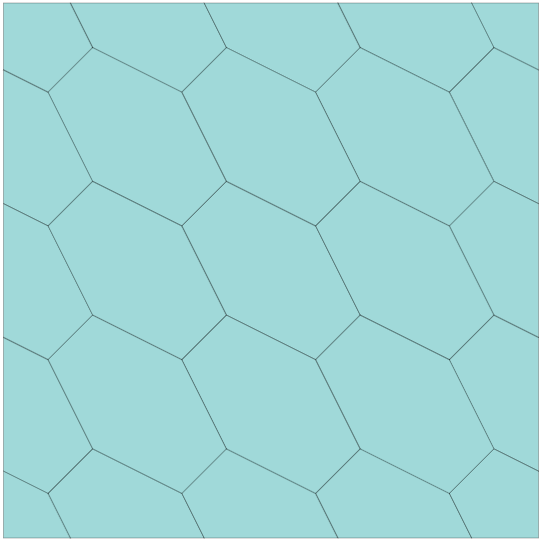

Figure 5: Representative two-dimensional polygonal meshes: convex polygonal mesh (left) and concave polygonal mesh (right)..
6.2 Two-dimensional biharmonic problem↩︎
Tables 1–2 report the errors for the biharmonic problem, corresponding to \(m=2\), on convex and concave polygonal meshes. The energy-type errors converge with order \(k+1\), and the \(L^2\) error \(\|u-u_0\|\) shows higher-order convergence.
| \(k\) | \(h\) | NT | \(\|\sigma-\sigma_h\|_{0,h}\) | Order | \(|u-u_0|_{H^2(\mathcal K_h)}\) | Order | \(\|u-u_0\|\) | Order |
|---|---|---|---|---|---|---|---|---|
| 0 | 1.250e-01 | 81 | 3.77e+00 | - | 1.85e+01 | - | 3.53e-03 | - |
| 6.250e-02 | 289 | 1.90e+00 | 0.99 | 9.51e+00 | 0.96 | 7.33e-04 | 2.27 | |
| 3.125e-02 | 1089 | 9.54e-01 | 0.99 | 4.79e+00 | 0.99 | 1.73e-04 | 2.08 | |
| 1.562e-02 | 4225 | 4.78e-01 | 1.00 | 2.40e+00 | 1.00 | 4.27e-05 | 2.02 | |
| 7.812e-03 | 16641 | 2.39e-01 | 1.00 | 1.20e+00 | 1.00 | 1.06e-05 | 2.00 | |
| 1 | 1.250e-01 | 81 | 9.28e-01 | - | 6.28e-01 | - | 1.93e-04 | - |
| 6.250e-02 | 289 | 2.38e-01 | 1.97 | 1.66e-01 | 1.92 | 1.26e-05 | 3.93 | |
| 3.125e-02 | 1089 | 5.96e-02 | 1.99 | 4.26e-02 | 1.96 | 8.06e-07 | 3.97 | |
| 1.562e-02 | 4225 | 1.49e-02 | 2.00 | 1.08e-02 | 1.98 | 5.09e-08 | 3.98 | |
| 7.812e-03 | 16641 | 3.73e-03 | 2.00 | 2.71e-03 | 1.99 | 3.21e-09 | 3.98 |
| \(k\) | \(h\) | NT | \(\|\sigma-\sigma_h\|_{0,h}\) | Order | \(|u-u_0|_{H^2(\mathcal K_h)}\) | Order | \(\|u-u_0\|\) | Order |
|---|---|---|---|---|---|---|---|---|
| 0 | 1.362e-01 | 64 | 2.00e+01 | - | 3.63e+00 | - | 1.89e-03 | - |
| 6.811e-02 | 256 | 1.01e+01 | 0.98 | 1.84e+00 | 0.98 | 2.54e-04 | 2.89 | |
| 3.405e-02 | 1024 | 5.08e+00 | 0.99 | 9.25e-01 | 0.99 | 7.00e-05 | 1.86 | |
| 1.703e-02 | 4096 | 2.54e+00 | 1.00 | 4.63e-01 | 1.00 | 2.07e-05 | 1.76 | |
| 8.513e-03 | 16384 | 1.27e+00 | 1.00 | 2.32e-01 | 1.00 | 5.67e-06 | 1.87 | |
| 1 | 1.362e-01 | 64 | 1.12e+00 | - | 6.80e-01 | - | 1.98e-04 | - |
| 6.811e-02 | 256 | 2.69e-01 | 2.05 | 1.73e-01 | 1.98 | 1.29e-05 | 3.94 | |
| 3.405e-02 | 1024 | 6.55e-02 | 2.04 | 4.33e-02 | 1.99 | 8.27e-07 | 3.97 | |
| 1.703e-02 | 4096 | 1.61e-02 | 2.02 | 1.08e-02 | 2.00 | 5.26e-08 | 3.97 | |
| 8.513e-03 | 16384 | 4.01e-03 | 2.01 | 2.71e-03 | 2.00 | 5.64e-09 | 3.22 |
6.3 Two-dimensional triharmonic problem↩︎
Tables 3–4 report the errors for the triharmonic problem, corresponding to \(m=3\), on convex and concave polygonal meshes. These tests include trace enrichment for \(k=0,1\), but no bubble enrichment is required because \(\lfloor m/\nu\rfloor=0\) for both mesh families. The energy-type errors converge with order \(k+1\), and the \(L^2\) error \(\|u-u_0\|\) shows higher-order convergence.
| \(k\) | \(h\) | NT | \(\|\sigma-\sigma_h\|_{0,h}\) | Order | \(|u-u_0|_{H^3(\mathcal K_h)}\) | Order | \(\|u-u_0\|\) | Order |
|---|---|---|---|---|---|---|---|---|
| 0 | 2.500e-01 | 25 | 8.34e+02 | - | 1.01e+02 | - | 1.13e-02 | - |
| 1.250e-01 | 81 | 3.92e+02 | 1.09 | 5.37e+01 | 0.91 | 1.24e-03 | 3.18 | |
| 6.250e-02 | 289 | 1.59e+02 | 1.30 | 2.73e+01 | 0.97 | 3.66e-04 | 1.76 | |
| 3.125e-02 | 1089 | 4.96e+01 | 1.68 | 1.38e+01 | 0.99 | 1.13e-04 | 1.69 | |
| 1.562e-02 | 4225 | 1.54e+01 | 1.68 | 6.91e+00 | 1.00 | 3.24e-05 | 1.81 | |
| 1 | 5.000e-01 | 9 | 1.55e+03 | - | 1.44e+02 | - | 7.58e-02 | - |
| 2.500e-01 | 25 | 3.83e+02 | 2.01 | 5.32e+01 | 1.43 | 3.02e-03 | 4.65 | |
| 1.250e-01 | 81 | 8.94e+01 | 2.10 | 1.45e+01 | 1.88 | 1.39e-04 | 4.45 | |
| 6.250e-02 | 289 | 2.71e+01 | 1.72 | 3.86e+00 | 1.91 | 9.22e-06 | 3.91 | |
| 3.125e-02 | 1089 | 7.48e+00 | 1.86 | 9.88e-01 | 1.96 | 6.29e-07 | 3.87 | |
| 2 | 5.000e-01 | 9 | 2.06e+03 | - | 8.51e+01 | - | 9.98e-03 | - |
| 2.500e-01 | 25 | 4.25e+02 | 2.28 | 1.77e+01 | 2.26 | 3.45e-04 | 4.85 | |
| 1.250e-01 | 81 | 5.51e+01 | 2.95 | 2.73e+00 | 2.70 | 9.34e-06 | 5.21 | |
| 6.250e-02 | 289 | 6.84e+00 | 3.01 | 3.66e-01 | 2.90 | 1.81e-07 | 5.69 | |
| 3.125e-02 | 1089 | 8.53e-01 | 3.00 | 4.70e-02 | 2.96 | 7.01e-09 | 4.69 |
| \(k\) | \(h\) | NT | \(\|\sigma-\sigma_h\|_{0,h}\) | Order | \(|u-u_0|_{H^3(\mathcal K_h)}\) | Order | \(\|u-u_0\|\) | Order |
|---|---|---|---|---|---|---|---|---|
| 0 | 2.724e-01 | 16 | 1.48e+03 | - | 1.04e+02 | - | 2.37e-02 | - |
| 1.362e-01 | 64 | 6.16e+02 | 1.27 | 5.47e+01 | 0.92 | 5.21e-03 | 2.19 | |
| 6.811e-02 | 256 | 2.08e+02 | 1.57 | 2.78e+01 | 0.98 | 1.16e-03 | 2.17 | |
| 3.405e-02 | 1024 | 7.58e+01 | 1.45 | 1.40e+01 | 0.99 | 2.83e-04 | 2.03 | |
| 1.703e-02 | 4096 | 3.29e+01 | 1.20 | 6.99e+00 | 1.00 | 7.86e-05 | 1.85 | |
| 1 | 5.449e-01 | 4 | 2.34e+03 | - | 1.49e+02 | - | 2.94e-01 | - |
| 2.724e-01 | 16 | 6.28e+02 | 1.90 | 5.20e+01 | 1.52 | 3.72e-03 | 6.30 | |
| 1.362e-01 | 64 | 1.31e+02 | 2.26 | 1.51e+01 | 1.78 | 1.90e-04 | 4.29 | |
| 6.811e-02 | 256 | 2.85e+01 | 2.20 | 3.93e+00 | 1.94 | 1.78e-05 | 3.42 | |
| 3.405e-02 | 1024 | 6.85e+00 | 2.06 | 9.92e-01 | 1.99 | 1.42e-06 | 3.64 | |
| 2 | 1.000e+00 | 1 | 2.74e+04 | - | 1.82e+02 | - | 2.40e-01 | - |
| 5.449e-01 | 4 | 5.13e+03 | 2.76 | 1.01e+02 | 0.98 | 7.82e-02 | 1.85 | |
| 2.724e-01 | 16 | 6.25e+02 | 3.04 | 1.83e+01 | 2.46 | 6.44e-04 | 6.92 | |
| 1.362e-01 | 64 | 7.79e+01 | 3.01 | 2.62e+00 | 2.80 | 1.13e-05 | 5.83 | |
| 6.811e-02 | 256 | 1.04e+01 | 2.90 | 3.35e-01 | 2.97 | 1.88e-07 | 5.91 |
6.4 Three-dimensional biharmonic problem↩︎
We also test the biharmonic problem in three dimensions on the unit cube \(\Omega=(0,1)^3\), with exact solution \[u(x,y,z)=\sin^2(\pi x)\sin^2(\pi y)\sin^2(\pi z).\] The domain is discretized by tetrahedral meshes. Although tetrahedra are simplicial elements rather than general polyhedra, they are polytopes and provide a useful three-dimensional test of the dimension-independent construction. For a tetrahedron, \(\nu=4\), and hence \(\left\lfloor\frac{m}{\nu}\right\rfloor = \left\lfloor\frac{2}{4}\right\rfloor =0.\) Thus no bubble enrichment is needed in this test. Table 5 shows that the method retains the predicted convergence behavior in three dimensions: the energy-type errors converge with order \(k+1\), and the \(L^2\) error shows higher-order convergence.
| \(k\) | \(h\) | NT | \(\|\sigma-\sigma_h\|_{0,h}\) | Order | \(|u-u_0|_{H^2(\mathcal K_h)}\) | Order | \(\|u-u_0\|\) | Order |
|---|---|---|---|---|---|---|---|---|
| 0 | 1.376e-01 | 384 | 1.43e+01 | - | 6.82e+00 | - | 4.40e-02 | - |
| 9.172e-02 | 1296 | 7.95e+00 | 1.45 | 4.46e+00 | 1.05 | 1.89e-02 | 2.09 | |
| 6.879e-02 | 3072 | 5.47e+00 | 1.30 | 3.32e+00 | 1.03 | 1.05e-02 | 2.03 | |
| 5.503e-02 | 6000 | 4.18e+00 | 1.21 | 2.64e+00 | 1.02 | 6.73e-03 | 2.01 | |
| 1 | 1.376e-01 | 384 | 9.86e+00 | - | 1.50e+00 | - | 3.93e-03 | - |
| 9.172e-02 | 1296 | 4.45e+00 | 1.96 | 6.80e-01 | 1.95 | 8.04e-04 | 3.91 | |
| 6.879e-02 | 3072 | 2.52e+00 | 1.98 | 3.85e-01 | 1.98 | 2.57e-04 | 3.96 | |
| 5.503e-02 | 6000 | 1.62e+00 | 1.99 | 2.47e-01 | 1.99 | 1.06e-04 | 3.98 |
References↩︎
The first author was partially supported by NSF grant DMS-2309785, the third author was supported by NSFC grant 12431014, and the fourth author was supported by NSFC grant 12401483.↩︎