Effective Stochastic Automata Model
Checking by Interval Abstraction1
(extended version)
January 01, 1970
Abstract
Stochastic automata (SA) are a formal stochastic continuous-time model based on countdown timers whose expiration times follow general probability distributions. SA are particularly useful to faithfully model and analyse dependable systems involving faults, maintenance, and repairs. Effective SA analysis approaches have so far been limited to statistical model checking and thus deterministic SA, while previously proposed model-checking techniques apply to limited subclasses of SA only, or do not scale. In this paper, we present the first dedicated SA model checking approach that is general and effective: It puts few restrictions on the input SA, and we show in our experimental evaluation that it works well for nontrivial examples. It combines a refinable interval abstraction of the continuous distributions with a direct application of the “big time steps” semantics of SA, providing upper/lower bounds on maximum/minimum reachability probabilities. We extend the Modest and Jani modelling formalisms with support for SA, and provide a prototype implementation of our approach in Rust.
1 Introduction↩︎
In dependable systems, component faults happen randomly over time, with schemes involving redundancy, regular inspections, maintenance, and repairs attempting to prevent escalation into overall system failure. Similarly, in high-performance systems, random queueing and service times, message loss probabilities, and signal transmission and propagation delays determine the system’s key performance properties such as throughput or response times. Formal models for dependability and performance evaluation [1] need to capture these aspects of stochastic time in a realistic way, as close as possible to the real system or the available data. Two widely-used formalisms are continuous-time Markov chains (CTMCs) and generalized stochastic Petri nets (GSPNs) [2], [3]. In both, all delays must be exponentially distributed. The resulting memoryless nature of these models admits scalable analytical analysis methods such as probabilistic model checking [4], [5]. In reality, however, many inter-event times are not exponentially distributed, and hard to approximate by CTMCs/phase-type distributions: time to failure is more realistically modelled by a Weibull distribution in most cases, and inspections typically happen around fixed intervals. We thus need non-Markovian formalisms that directly incorporate general continuous probability distributions, such as stochastic automata (SA) [6] or Petri nets with general transitions (e.g. HPnGs [7]). In this paper, we use SA, because they are conceptually simple yet highly expressive. Additionally, their compositionality makes them attractive for modelling complex component-based systems.
SA extend labelled transition systems with stochastic timers (that may be reset to values sampled from continuous probability distributions to then decrease over time and expire when reaching value zero) and guard sets that enable an edge when all their timers have expired. As SA are non-Markovian and allow nondeterministic choices, their analysis is hard. The only available tool with dedicated SA support, Fig [8], employs statistical model checking [9], [10] (i.e. Monte Carlo simulation) and is thus restricted to (weakly) deterministic SA [11]. Analytical approaches for more general models, such as HPnGs or stochastic timed automata (STA) [12], [13], do not scale for typical SA that have many discrete locations and several timers possibly reset repeatedly on loops.
We present the first dedicated model checking approach for SA that is effective (i.e. works for typical and nontrivial SA models) and implemented in an available tool. It is based on interval abstraction [14]: we replace each clock reset, i.e. each sampling from a continuous distribution \(\mu\), by a discrete distribution over a finite set of intervals that partition \(\mu\)’s support. The choice of concrete value from an interval is nondeterministic, and we propagate the intervals symbolically through the semantics of the SA. This turns the SA into a Markov decision process (MDP) [15], [16] that overapproximates the SA’s semantics. As a result, the max.(min.) probability of eventually reaching a set of MDP states corresponding to a goal location in the SA—which we compute by value iteration [17]—is an upper (lower) bound on the corresponding probability in the SA.
We specify our approach formally and show the overapproximation property (3). We extend the Modest [12], [18] and Jani [19] languages with support for timers and thus SA, providing a new user-friendly high-level modelling language for SA and a means to conveniently exchange SA models between tools (4). Our new SA model checking approach is implemented in a prototype tool written in Rust, which we use to evaluate its performance and scalability characteristics on example SA from and inspired by the literature (5). We find that, despite its prototypical nature, our tool already works well for reasonably-sized SA even when using many intervals to obtain results with good accuracy.
1.0.0.1 Related work.
Fig’s simulation-based approach (mentioned above) is limited to a subclass of input-output SA that syntactically guarantees all nondeterminism to be spurious, i.e. minimum and maximum reachability probabilities coincide.
Two SA model checking algorithms were proposed by Bryans et al. in 2003 [20]. They use a clock-based variant of SA with severe restrictions (clocks may only be used out of locations in which they have just been reset, and all distributions must be non-negative and bounded). The first algorithm uses a “region tree” and requires solving nested integrals over the probability density functions of each expired clock, which becomes infeasible as the tree grows in depth. The second algorithm avoids the nested integrals by discretising the distributions. No tool implements either algorithm today. We note that our interval abstraction does not discretise the sampling results, but instead replaces continuous probabilistic choices by discrete probabilistic followed by continuous nondeterministic ones. For nondeterministic SA, both algorithms require a strategy to be user-specified, while our approach includes the optimisation over nondeterministic choices.
Model checking tool support exists for the following stochastic-timed formalisms that are more general than SA: (1) STA extend timed automata by allowing clocks to be compared to real-valued variables whose values can be sampled from general probability distributions. Compared to SA, they also support continuous nondeterministic delays, and are very (unrealistically) flexible in how clocks and the real-valued variables can be combined. Interval abstraction has been implemented for STA in the Modest Toolset’s [21] mcsta model checker [13] in a way that reduces the STA to a probabilistic timed automaton [22], which is turned into an MDP via the digital clocks approach [23], [24]. The implementation is limited to abstraction intervals of width 1 (or infinity). The digital clocks semantics enumerates all time steps of duration 1, making the MDP very large, but also preventing refinement to smaller intervals. (2) Stochastic hybrid automata (SHA) [14] further extend STA with continuous variables whose evolution over time is governed by differential equations and inclusions. The prohver tool applies interval abstraction to SHA, followed by a hybrid reachability analysis via Phaver [25], to overapproximate reachability probabilities. Here, the abstraction intervals have to be specified manually by the user, and the hybrid reachability step—unnecessary for SA—is the scalability and performance bottleneck. (3) While prohver applies to linear SHA of type I, the Realyst tool [26] focuses on rectangular hybrid automata with random events (RAEs), into which (some) SA can also be encoded. Realyst’s approach works for time-bounded reachability only, and requires structurally non-Zeno RAEs, which complicates the analysis of SA with cycles. As every timer reset must be encoded as a separate random variable in the RAE, each of which Realyst turns into one dimension of the model’s continuous state, scalability—already limited by the complexity of hybrid reachability—for typical SA is low.
Finally, Buchholz et al. [27] present model checking algorithms for a generalization of CTMCs with clocks that they also call “stochastic automata”, but clearly point out that their definition is less general than the one of [6] that we use.
2 Background↩︎
Let \(\mathbb{R}_{\geqslant 0}\) be \([0, \infty)\), \(\mathbb{R}_{>0}\mathrel{\vbox{\offinterlineskip\ialign{\hfil##\hfil\cr{\tiny \rm def}\cr\noalign{\kern 0.30ex}=\cr}}}(0, \infty)\), and \(\mathbb{R}_\infty \mathrel{\vbox{\offinterlineskip\ialign{\hfil##\hfil\cr{\tiny \rm def}\cr\noalign{\kern 0.30ex}=\cr}}}\mathbb{R}\cup \{\,\infty\,\}\). A discrete probability distribution is a function \(\mu\colon S \to [0,1]\) over a countable set \(S\) with \(\sum_{s \in S}\mu(s) = 1\). Its support is \(\mathit{spt}({\mu}) \mathrel{\vbox{\offinterlineskip\ialign{\hfil##\hfil\cr{\tiny \rm def}\cr\noalign{\kern 0.30ex}=\cr}}}\{\, s \in S | \mu(s) > 0\,\}\). Now let \(S\) be an arbitrary set. We write \(\mathcal{P}({S})\) for its powerset. Given a \(\sigma\)-algebra \(\sigma(S)\) over \(S\), subset \(A \subseteq S\) is measurable if \(A \in \sigma(S)\). A probability measure over \(S\) is a function \(\mu\colon \sigma(S) \to [0,1]\) with \(\mu(S) = 1\) and \(\mu(\bigcup_{i \in I}A_i) = \sum_{i \in I} \mu(A_i)\) for any countable index set \(I\) and measurable pairwise disjoint \(A_i \subseteq S\). The support of probability measure \(\mu\) is the smallest compact (measurable) set \(\mathit{spt}({\mu}) \subseteq S\) s.t.\(\mu(\mathit{spt}({\mu}))=1\). Given two probability measures \(\mu_1\) and \(\mu_2\) over \(S\), the product measure is the unique probability measure such that \((\mu_1 \otimes \mu_2) (A_1 \times A_2) = \mu_1(A_1) \cdot \mu_2 (A_2)\) for all measurable \(A_1, A_2 \subseteq S\). A probability measure \(\mu\) over \(\mathbb{R}\) is absolutely continuous if \(\mu(A) = 0\) for all \(A\) of Lebesgue measure \(0\); we call it a continuous probability distribution (CPD). \(\mathit{DPD}({S})\) is the set of all discrete probability distributions, \(\mathit{PD}({S})\) of all probability measures, and \(\mathit{CPD}({S})\) of all CPDs over appropriate \(S\).
2.0.0.1 Stochastic automata
[6], [28] are labelled transition systems equipped with timers: real-valued variables that can be reset to values sampled from CPDs, decrease synchronously with time, and guard the SA’s edges. Formally:
Definition 1. A stochastic automaton* (SA) is a tuple \(\langle \mathcal{L}, \ell_I, \mathcal{A}, \mathcal{V}, \mathcal{E} \rangle\) consisting of finite sets of locations \(\mathcal{L}\) with initial location \(\ell_I\in \mathcal{L}\), action labels \(\mathcal{A}\) with \(\mathcal{A}\cap \mathbb{R}= \varnothing\), timer variables \(\mathcal{V}\), and edges \(\mathcal{E}\subseteq \mathcal{L}\times \mathcal{P}({\mathcal{V}}) \times \mathcal{A}\times \mathcal{P}({\mathcal{V}}) \times \mathcal{L}\). Each timer \(x\) has an associated CPD \(\mu_x\) with \(\mu_x(\mathbb{R}_{\geqslant 0}) = 1\). We write \(\ell \xrightarrow{{\raisebox{-1pt}[0pt][0pt]{\scriptstyle{G, a, R}}}} \ell'\) for \(\langle \ell, G, a, R, \ell' \rangle \in \mathcal{E}\); such an edge consists of a source location \(\ell\), a guard set \(G \subseteq \mathcal{V}\), an action \(a \in \mathcal{A}\), a reset set \(R \subseteq \mathcal{V}\), and a target location \(\ell'\).*
Unless noted otherwise, we assume SA \(\mathcal{M} = \langle \mathcal{L}, \ell_I, \mathcal{A}, \mathcal{V}, \mathcal{E} \rangle\) to be given in the remainder of this paper. Let \(\vec{v}\colon \mathcal{V}\to \mathbb{R}\) be a timer valuation. Let valuation \(\vec{0}\) be defined by, for all \(t \in \mathcal{V}\), \(\vec{0}(t) = 0\), and \(\vec{v} - d\) for \(d \in \mathbb{R}\) by \((\vec{v} - d)(t) = v(t) - d\). In an SA’s semantics, we start in \(\ell_I\) with all timers having value \(0\). When in location \(\ell\), all timers synchronously decrease at rate \(1\) over time. If \(\ell \xrightarrow{{\raisebox{-1pt}[0pt][0pt]{\scriptstyle{G, a, R}}}} \ell'\) and all timers in \(g\) have expired (i.e. have value \(\leq 0\)), then no further time can pass (maximal progress), and the edge must be taken: the timers in \(R\) are reset (i.e. assigned a new value randomly sampled from their associated CPD), and we continue in location \(\ell'\). The semantics also allows discrete nondeterministic choices between edges if there is another edge whose guard’s timers have all expired. Formally, it is given in terms of an infinite-state but finitely branching transition system:
Definition 2. A timed probabilistic transition system* (TPTS) is defined as a tuple \(\langle \mathcal{S}, s_I, \mathcal{A}', \mathcal{T} \rangle\) consisting of a measurable set of states \(\mathcal{S}\) with initial state \(s_I\in \mathcal{S}\), an alphabet \(\mathcal{A}' = \mathbb{R}_{>0}\uplus \mathcal{A}\) partitioned into delays in \(\mathbb{R}_{>0}\) and actions in \(\mathcal{A}\), and transitions \(\mathcal{T}\subseteq \mathcal{S}\times \mathcal{A}' \times \mathit{PD}({\mathcal{S}})\). We write \(s \xrightarrow{{\raisebox{-1pt}[0pt][0pt]{\scriptstyle{\alpha}}}} \mu\) for \(\langle s, \alpha, \mu \rangle \in \mathcal{T}\); such a transition consists of a source state \(s\), label \(\alpha \in \mathcal{A}'\), and measure over target states \(\mu\). For all \(s \in \mathcal{S}\), we require \(\mathcal{T}_s \mathrel{\vbox{\offinterlineskip\ialign{\hfil##\hfil\cr{\tiny \rm def}\cr\noalign{\kern 0.30ex}=\cr}}}\{\, \langle s, \alpha, \mu \rangle \in \mathcal{T}\,\}\) to be finite and \(|\mathcal{T}_s| = 1\) if \(\exists\,\langle s, d, \mu \rangle \in \mathcal{T}\colon d \in \mathbb{R}_{>0}\) (i.e. states admitting delays are deterministic).*
Definition 3. The TPTS \(\llbracket{M}\rrbracket \mathrel{\vbox{\offinterlineskip\ialign{\hfil##\hfil\cr{\tiny \rm def}\cr\noalign{\kern 0.30ex}=\cr}}}\langle \mathcal{L}\times (\mathcal{V}\to \mathbb{R}_\infty), \langle \ell_I, \vec{0} \rangle, \mathcal{A}\cup \mathbb{R}_{>0}, \mathcal{T}_{\llbracket{M}\rrbracket} \rangle\) is the semantics of an SA* \(\mathcal{M}\) with \(\mathcal{T}_{\llbracket{M}\rrbracket}\) being the smallest relation satisfying \[\begin{gather} \frac{ \ell \xrightarrow{G, a, R} \ell' \quad \bigwedge_{x_i \in G}{\vec{v}(x_i)\leq 0} }{ \langle \ell, \vec{v} \rangle \xrightarrow{a} \{\,s' \mapsto 1\,\} \otimes \left(\bigotimes_{x_i \in R}\mu_{x_i}\right) \otimes \left(\bigotimes_{x_i \notin R} \{\,\vec{v}(x_i) \mapsto 1\,\}\right) } \quad(\mathrm{S1}) \\[2pt] \text{and}\quad \frac{ 0 < d = \min\{\,\max\{\, \vec{v}(x_i)\mid x_i \in G \,\} \mid \ell \xrightarrow{G, a, R} \ell'\,\} }{ \langle \ell, \vec{v} \rangle \xrightarrow{d} \{\,\langle \ell, \vec{v} - d \rangle \mapsto 1\,\} } \quad(\mathrm{S2}) \end{gather}\] with all resulting deadlock states receiving an \(\infty\)-labelled self-loop.*
This definition is the “big time steps” semantics of SA [29]: Rule S2 admits only the delay that directly enables an edge, and no intermediate delays as in other “dense time steps” semantics. For the closed SA and properties we use, the two semantics are equivalent (in essence, weakly bisimilar in a time-abstract way).
Figure 1: 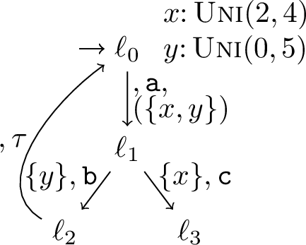 .
.
Example 1. [fig:sa95running95example] shows our running example SA \(\mathcal{M}_\mathit{re}\). It has two timers \(x\) and \(y\) whose expiration times are sampled from the given uniform distributions. The two edges labelled
a and \(\tau\) out of locations \(\ell_0\) and \(\ell_2\) have empty guard sets: they must be taken immediately upon entering those locations.
In \(\ell_1\), the outgoing edges can only and must be taken when the respective timer has expired. If \(y\) expires before \(x\), we go to \(\ell_2\), and to \(\ell_3\) otherwise. Timers are only reset on the edge from \(\ell_0\) to \(\ell_1\) as denoted by the reset
set \(\text{R}(\{ x, y \})\). We omit empty reset sets.
In general, SA are compositional: They can be equipped with a notion of parallel composition and an open semantics with dense time steps and without maximal progress. This facilitates elegant and compact models of systems consisting of concurrent components. For analysis, usually the composition’s closed semantics which excludes parallel composition and synchronization on shared actions between SA is considered, and thus we use single closed SA in this paper.
2.0.0.2 Properties.
Given an SA, we are interested in the probability of reaching any of a set of goal locations \(\mathcal{G} \subseteq \mathcal{L}\), defined via the probability of reaching any state in \(\llbracket{\mathcal{G}}\rrbracket \mathrel{\vbox{\offinterlineskip\ialign{\hfil##\hfil\cr{\tiny \rm def}\cr\noalign{\kern 0.30ex}=\cr}}}\{\, \langle \ell, \vec{v} \rangle \mid \ell \in \mathcal{G} \,\}\) in the TPTS semantics. In a TPTS, a path is an infinite sequence \(s_0 \langle a_0, \mu_0 \rangle s_1 \langle a_1, \mu_1 \rangle \!\ldots \in (\mathcal{S}\times (\mathcal{A}' \times \mathit{PD}({\mathcal{S}})))^\omega\) with \(s_0 = s_I\) and \(\forall i\colon s_i \xrightarrow{{\raisebox{-1pt}[0pt][0pt]{\scriptstyle{a_i}}}} \mu_i \wedge s_{i+1} \in \mathit{spt}({\mu_i})\). Paths resolve all nondeterministic and probabilistic choices. A strategy resolves only the nondeterminism:
Definition 4. \(\mathfrak{s}\colon \mathcal{S}\to \mathcal{A}' \times \mathit{PD}({\mathcal{S}})\) is a strategy* if \(\mathfrak{s}(s) = \langle \alpha, \mu \rangle \Rightarrow s \xrightarrow{{\raisebox{-1pt}[0pt][0pt]{\scriptstyle{\alpha}}}} \mu\).*
We work with memoryless deterministic strategies. Randomised ones would be needed for e.g. multi-objective properties [30], and for reachability properties on SA, memoryless and history-dependent strategies are equally expressive [29].
Every strategy \(\mathfrak{s}\) induces a probability measure \(\mathbb{P}_{\!\mathfrak{s}}\) on the space of all paths. For a formal definition, see [31]. As is usual, we restrict to non-Zeno strategies: we require \(\mathbb{P}_{\!\mathfrak{s}}(\Pi_\infty) = 1\), where \(\Pi_\infty\) is the set of paths whose sum of delays is \(\infty\).
Definition 5. Consider a TPTS that is the semantics of an SA with goal set \(\mathcal{G} \subseteq \mathcal{L}\). Then \(\mathrm{P}_\mathrm{\!min}(\diamond\,\mathcal{G})\) and \(\mathrm{P}_\mathrm{\!max}(\diamond\,\mathcal{G})\) are the minimum and maximum reachability probabilities* for \(\mathcal{G}\), defined as \(\mathrm{P}_\mathrm{\!min}(\diamond\,\mathcal{G}) = \inf_{\mathfrak{s}} \mathbb{P}_{\!\mathfrak{s}}(\lozenge_\mathcal{G})\) and \(\mathrm{P}_\mathrm{\!max}(\diamond\,\mathcal{G}) = \sup_{\mathfrak{s}} \mathbb{P}_{\!\mathfrak{s}}(\lozenge_\mathcal{G})\), respectively, with \(\lozenge_\mathcal{G}\) the set of paths that contain a state in \(\llbracket{\mathcal{G}}\rrbracket\).*
2.0.0.3 Markov decision processes
are finite TPTSs whose transitions lead into discrete probability distributions. They are the result of interval abstraction of SA.
Definition 6. A Markov decision process* (MDP) is a tuple \(\langle \mathcal{S}, s_I, \mathcal{A}, \mathcal{T} \rangle\) with finite sets of states \(\mathcal{S}\) with initial state \(s_I\in \mathcal{S}\), action labels \(\mathcal{A}\), and transitions \(\mathcal{T}\subseteq \mathcal{S}\times \mathcal{A}\times \mathit{DPD}({\mathcal{S}})\). For all \(s \in \mathcal{S}\), we require non-empty \(\mathcal{T}_s \mathrel{\vbox{\offinterlineskip\ialign{\hfil##\hfil\cr{\tiny \rm def}\cr\noalign{\kern 0.30ex}=\cr}}}\{\, \langle s, \alpha, \mu \rangle \in \mathcal{T}\,\}\).*
We can define reachability probabilities for MDPs in a similar way as for TPTSs. On MDPs, they can be computed or approximated efficiently via linear programming, policy iteration, or various variants of value iteration (VI) [17].
3 Big-Steps Interval Abstraction for SA↩︎
Interval abstraction of models with continuous probability distributions was introduced for the analysis of SHA [14], where it turned the SHA into a probabilistic hybrid automaton (PHA) [32], [33], which could in turn be analysed by combining a hybrid reachability checker with MDP model checking. Interval abstraction replaces sampling from a CPD \(\mu\) by a combination of (1) discrete sampling from a finite set of intervals that partition (or, in general, cover) \(\mathit{spt}({\mu})\), with interval \(I_i\) chosen with probability \(\mu(I_i)\), followed by (2) a continuous nondeterministic choice to choose a concrete value from the sampled interval. Interval abstraction does not discretise the final outcome: Every value in \(\mathit{spt}({\mu})\) can still be chosen, but instead of being fully random, the strategy now makes the choice within the sampled interval. Since we use absolutely continuous distributions, we can neglect singleton overlaps between the intervals (as they have probability \(0\)), and will thus use closed intervals throughout. The intervals to use for the abstraction can be specified in different ways. In our implementation and examples, we specify the desired probability mass of each interval, but we could equally specify the interval width or just the intervals themselves.
Example 2. When abstracting uniform distribution \(\mathrm{\small Uni}(0, 5)\) from 1 with per-interval probability of \(0.5\), we obtain intervals \([0, 2.5]\) and \([2.5, 5]\). For \(\mathrm{\small Exp}(1)\), the exponential distribution with rate \(1\), we obtain \([0, -{\ln 0.5}]\) and \([-{\ln 0.5}, \infty)\).
We apply interval abstraction to the semantics of 3, but then propagate the intervals symbolically. We thus avoid (in effect: postpone) the explicit continuous nondeterministic choices and obtain a finite MDP. In this section, we specify our transformation formally and establish its relation to the TPTS semantics.
3.1 SA Interval Abstraction↩︎
Let \(\mathfrak{I}\) denote the set of all closed intervals in \(\mathbb{R}_{\geqslant 0}^{\infty}\) together with all intervals of the form \([l,\infty)\). Given interval \(I\), let \(lI=\inf(I)\) and \(uI=\sup(I)\). A set of intervals \(B\subseteq\mathfrak{I}\) is non-overlapping if for all \(I_1,I_2\in B\), \(I_1\cap I_2\neq\varnothing\) implies either \(uI_1=lI_2\) or \(uI_2=lI_1\). Let \(\mathscr{P}_{\mathrm{nol}}(\mathfrak{I})\) be the set of all non-overlapping subsets of \(\mathfrak{I}\). A timer-domain partition is a function \(\mathfrak{p}\colon \mathcal{V}\to \mathscr{P}_{\mathrm{nol}}(\mathfrak{I})\) s.t.for all \(x\in\mathcal{V}\), \(\bigcup {\mathfrak{p}(x)} = \mathit{spt}({\mu_x})\).
Given an SA \(\mathcal{M}\) as usual and a timer-domain partition \(\mathfrak{p}\), we define its interval abstraction as the MDP \(\mathsf{ia}(\mathcal{M})=(S_\mathsf{ia}, \langle \ell_I, \vec{0}_\mathsf{ia} \rangle, \mathcal{A}\cup \{\,\sigma\,\}, \mathcal{T}_\mathsf{ia})\) where
\(\sigma\notin\mathcal{A}\) is a fresh new label indicating some unspecified sojourn time;
\(S_\mathsf{ia}= \mathcal{L}\times (\mathcal{V}\to \mathfrak{I}\cup \{\,\lightning\,\})\) where, for each state \(\langle \ell, b \rangle \in S_\mathsf{ia}\) and \(x \in \mathcal{V}\), if \(b(x)=\lightning\), timer \(x\) has already expired in this state and, otherwise, \(b(x)\) is the interval containing all possible values timer \(x\) can take in this state with \(lb(x)\) and \(ub(x)\) denoting the interval’s lower and upper bound, respectively, and for a set \(C\subseteq\mathcal{V}\) of timers, we let \(lb(C)=\max\{\,lb(x)\mid x\in C \wedge b(x)\neq\lightning\,\}\) (the delay after which all timers can have expired) and \(ub(C)=\max\{\,ub(x)\mid x\in C \wedge b(x)\neq\lightning\,\}\) (the delay after which all timers must have expired);
\(\vec{0}_\mathsf{ia}\) maps every timer to \(\lightning\) in the initial state; and
\(\mathcal{T}_\mathsf{ia}\) is the smallest relation satisfying the following two inference rules: \[\frac{ \ell \xrightarrow{G, a, R} \ell' \quad \forall x \in G\colon b(x) = \lightning }{ \langle \ell,b \rangle \xrightarrow{a} \pi^b_{R, \ell'} } \qquad(\text{R1})\] with the transitions’ target distributions defined by \[\pi^b_{R, \ell'}(\langle \ell'', b' \rangle)= \begin{cases} \displaystyle\prod_{x \in R}\mu_x(b'(x)) & \text{if } \begin{array}[t]{l} \ell''=\ell',\\ \forall{x \notin R}\colon b'(x)=b(x), \text{ and}\\ \forall{x \in R}\colon b'(x)\in\mathfrak{p}(x) \end{array} \\ 0 & \text{otherwise} \end{cases}\] and \[\frac{ \ell \xrightarrow{G, a, R} \ell' \quad \forall \ell \xrightarrow{G'\!\!,\,a'\!\!,\,R'} \ell'' \colon (\exists\, x \in G'\colon b(x) \neq \lightning) \wedge lb(G) \leq ub(G') }{ \langle \ell, b \rangle \xrightarrow{\sigma} \{\, \langle \ell, d_{\ell, G}^b \rangle \mapsto 1 \,\} } \qquad(\text{R2})\] with \[d_{\ell, G}^b(x)= \begin{cases} \lightning&\hfill\makebox[0em][r]{if x \in G \vee b(x)=\lightning\vee ub(x) \leq lb(G)}\\[1ex] \Big[ \max\{ 0, lb(x) {-} \min\{ ub(G') \mid \ell \xrightarrow{G'\!\!,\,a'\!\!,\,R'} \ell'' \}\}, ub(x) {-} lb(G) \Big] &\text{else} \end{cases}\] with all resulting deadlock states receiving a \(\sigma\)-labelled self-loop.
Rule R1 creates an MDP transition to \(\pi^b_{R, \ell'}\) whenever an edge in the SA would be enabled in the current state; the discrete distribution \(\pi^b_{R, \ell'}\) samples an interval for every timer that is reset. Rule R2 creates \(\sigma\)-labelled transitions, which represent the symbolic passage of some time, as follows:
The rule picks an edge \(e = \ell \xrightarrow{{\raisebox{-1pt}[0pt][0pt]{\scriptstyle{G, a, R}}}} \ell'\) out of the current location \(\ell\) in the SA that should become enabled. If \(\ell\) has no edges, then no symbolic time passes.
First, no edge must be enabled in the current state—otherwise, by maximal progress, it would have to be taken immediately. This is condition “\(\exists\, x \in G'\colon b(x) \neq \lightning\)”: In every guard set, at least one timer is not expired.
Additionally, no edge may be forced to be taken earlier. This is condition “\(lb(G) \leq ub(G')\)”: else, edge \(e'\) with guard \(G'\) must be taken after waiting for \(ub(G')\) time units, while \(e\) needs at least delay \(lb(G) > ub(G')\) to be enabled.
If these conditions hold, then all timers in \(G\) can expire, and we let them do so. Function \(d_{\ell, G}^b\) determines the new intervals of values that all timers not in \(G\) can then be in: The first case states that all timers are expired (\(\lightning\)) that (i) are in \(G\), (ii) have previously expired, or (iii) whose upper bound is at most \(lb(G)\) (which applies to timers not in \(G\) that have “low” values). In the second case, we have an unexpired timer \(x \notin G\) that is not forced to expire now. Its lower bound is reduced by the maximum amount of time that could have passed, which is the lowest upper bound of the guard set of any edge out of \(\ell\), but not below \(0\). If the new lower bound is \(0\), \(x\) could have expired, but since \(x \notin G\), it by choice did not expire.2 The upper bound, in turn, is decreased by the lowest possible delay needed for all timers in \(G\) to expire.
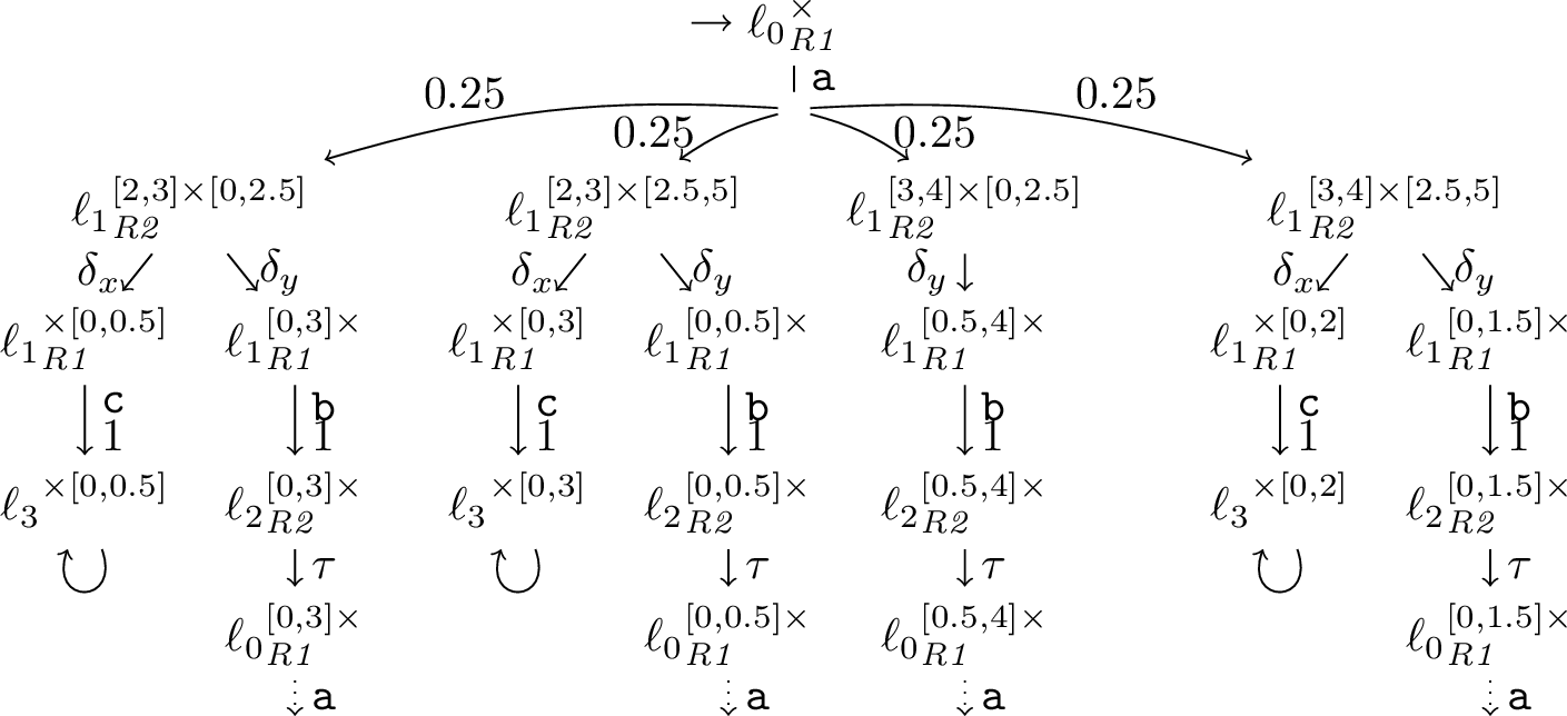
Example 3. Applying interval abstraction to \(\mathcal{M}_\mathit{re}\) of 1 with a per-interval probability
of \(0.5\) results in the MDP of which an excerpt is shown in 2. In \(\ell_0\), initially, all timers are expired, so the
a-labelled edge in the SA can be taken. It resets both timers, thus the corresponding transition in the MDP as per R1 leads to a distribution over the four combinations of intervals for \(x\) and \(y\).
Location \(\ell_1\) has two edges, with two distinct non-empty guards, \(\{\,y\,\}\) and \(\{\,x\,\}\). By R2, we get up to two \(\sigma\)-labelled transitions out of each state in the second row of 1. For clarity, we instead label the ones where \(\{\,y\,\}\) (\(\{\,x\,\}\)) was chosen to expire with \(\delta_y\) (\(\delta_x\)). Note that in \({\ell_1}^{[3,4] \times [0, 2.5]}_\mathit{R2}\), only the expiration of \(\{\,y\,\}\) is considered because the expiration of \(\{\,x\,\}\) would violate the “\(lb(G) \leq ub(G')\)” requirement: \(ub(\{\,y\,\}) = 2.5 \leq lb(\{\,x\,\}) = 3\), i.e. \(y\) must* expire before \(x\).*
In the third row, the timers of the chosen guard set have expired, and the corresponding SA edge labelled b or c can be taken as per R1. Observe that timers not in the chosen guard set may have lower bound \(0\) now but are not considered expired, as explained earlier; thus e.g. in state \({\ell_1}^{[0,0.5] \times \lightning}_\mathit{R1}\) only the b-labelled transition is possible
despite \(lb(x) = 0\).
Finally, in the fourth row, we can either loop back to \(\ell_0\) from \(\ell_2\), or else we are stuck in \(\ell_3\). In the former case, the
a-labelled transitions reset both timers, and thus lead into the same distribution (not shown in 1) as the a-labelled transition out of the
initial state, looping back into the second row. 1 thus includes all 23 states of the interval abstraction and all transitions.
3.2 Correctness↩︎
In order to check the optimal probability of reaching a location \(\ell\) (or a set of locations) in the SA, we compute the optimal probability of reaching a state \(\langle \ell, g \rangle\) for any \(g\) in the interval abstraction MDP (see 2). Since the SA is finite, and the abstraction intervals are fixed for every timer, this MDP must also be finite—but it can be large when many different combinations of (post-delay) intervals can be reached. MDP model checking, however, has good practical scalability, solving models of hundreds of millions of states on standard hardware today.
The interval abstraction does not preserve reachability probabilities exactly, however; it rather introduces an overapproximation from two sources: First, MDP strategies can choose the precise value to use within the intervals whereas this choice is fully random in the SA semantics. Second, this choice is actually postponed from the moment the edge that does the sampling is taken to the point that one of the transitions generated by R2 must be chosen. This moves nondeterministic choices over (other) probabilistic choices, which also gives more information to the strategies.3 Thus maximum (minimum) reachability probabilities in the MDP overapproximate (underapproximate) the corresponding probabilities in the SA’s semantics:
Theorem 1. Given an SA \(\mathcal{M}\) as usual and a set of goal locations \(\mathcal{G} \subseteq \mathcal{L}\), let \(p_\mathit{min}^\mathcal{M} = \mathrm{P}_\mathrm{\!min}(\diamond\,\mathcal{G})\) and \(p_\mathit{max}^\mathcal{M} = \mathrm{P}_\mathrm{\!max}(\diamond\,\mathcal{G})\) be the optimal reachability probabilities obtained from \(\llbracket{\mathcal{M}}\rrbracket\) as per 5, and let \(p_\mathit{min}^{\mathsf{ia}(\mathcal{M})}\) and \(p_\mathit{max}^{\mathsf{ia}(\mathcal{M})}\) be the analogous probabilities obtained from the MDP \(\mathsf{ia}(\mathcal{M})\). Then \[p_\mathit{min}^{\mathsf{ia}(\mathcal{M})} \leq p_\mathit{min}^\mathcal{M} \qquad\text{and}\qquad p_\mathit{max}^\mathcal{M} \leq p_\mathit{max}^{\mathsf{ia}(\mathcal{M})}.\]
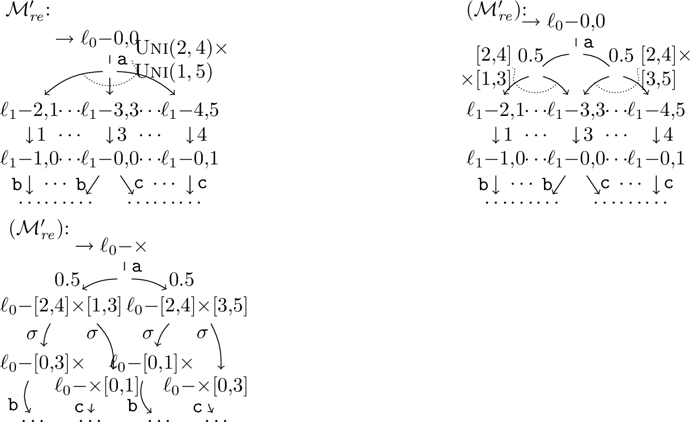
sketch. Our proof is inspired by that of [34]. We illustrate the idea with a variant \(\mathcal{M}_\mathit{re}'\) of \(\mathcal{M}_\mathit{re}\) from [fig:sa95running95example] with CPDs slightly simplified to \(x\colon \mathrm{\small Uni}(2, 4)\) and \(y\colon \mathrm{\small Uni}(1, 3)\), and abstraction intervals \(\mathfrak{p}_\mathit{re}'(x) = \{\, [2,4] \,\}\) and \(\mathfrak{p}_\mathit{re}'(y) = \{\, [1,3], [3, 5] \,\}\). We show an excerpt of \(\llbracket{\mathcal{M}_\mathit{re}'}\rrbracket\) on the left of 3.
The interval abstraction directly maps an SA \(\mathcal{M}\) to the MDP \(\mathsf{ia}(\mathcal{M})\). We introduce an intermediate step: an interval abstraction \(\mathsf{ia}(\llbracket{\mathcal{M}}\rrbracket)\) of \(\llbracket{\mathcal{M}}\rrbracket\) over the same \(\mathfrak{p}\). It is obtained from \(\llbracket{\mathcal{M}}\rrbracket\) by replacing each continuous distribution \(\mu_{x_i}\) in rule \(\mathrm{S1}\) of 3 by a discrete distribution \(\mu_{x_i}^\mathsf{ia}\) over the intervals in \(\mathfrak{p}(x_i)\) followed by a continuous nondeterministic selection of a concrete value from the chosen interval such that \(\mu_{x_i}^\mathsf{ia}(I) = \mu_{x_i}(I)\). We show \(\mathsf{ia}(\llbracket{\mathcal{M}}\rrbracket_\mathit{re}')\) in the middle of 3. Where a transition in \(\llbracket{\mathcal{M}}\rrbracket\) leads into a continuous distribution over states, in \(\mathsf{ia}(\llbracket{\mathcal{M}}\rrbracket)\), it now leads into a discrete distribution (solid dot ) over sets of states out of which one is chosen nondeterministically (outlined dots ).
The (reachable) states of \(\llbracket{\mathcal{M}}\rrbracket\) and \(\mathsf{ia}(\llbracket{\mathcal{M}}\rrbracket)\) are the same, as is the transition graph structure. Given a strategy \(\mathfrak{s}\) for \(\llbracket{\mathcal{M}}\rrbracket\), we can construct a randomised strategy \(\mathfrak{s}_{\llbracket{\mathsf{ia}}\rrbracket}\) for \(\mathsf{ia}(\llbracket{\mathcal{M}}\rrbracket)\) that induces the exact same probability measure: First, fix \(\mathfrak{s}(s) = \mathfrak{s}_{\llbracket{\mathsf{ia}}\rrbracket}(s)\) for all states \(s\). Then, \(\mathfrak{s}_{\llbracket{\mathsf{ia}}\rrbracket}\) resolves all the new continuous nondeterministic choices of values from intervals randomly so that \(\mathfrak{s}_{\llbracket{\mathsf{ia}}\rrbracket} \circ \mu_{x_i}^\mathsf{ia}= \mu_{x_i}\) everywhere. This is possible because \(\mu_{x_i}^\mathsf{ia}\) and \(\mu_{x_i}\) assign the same probabilities to all these intervals. \(\mathsf{ia}(\llbracket{\mathcal{M}}\rrbracket)\) may have additional strategies not corresponding to any in \(\llbracket{\mathcal{M}}\rrbracket\), and we thus have \(p_\mathit{min}^{\mathsf{ia}(\llbracket{\mathcal{M}}\rrbracket)} \leq p_\mathit{min}^\mathcal{M}\) and \(p_\mathit{max}^\mathcal{M} \leq p_\mathit{max}^{\mathsf{ia}(\llbracket{\mathcal{M}}\rrbracket)}\).
Observe that, by rule \(\mathrm{S2}\) of 3, \(\mathsf{ia}(\llbracket{\mathcal{M}}\rrbracket)\) contains no nondeterminism over delays, delay transitions are deterministic, and only connect states that are in the same SA location. We can thus collapse all delay transitions, i.e. delete them and copy the outgoing transitions of their successor states onto their source states, without affecting the trace distributions modulo delay steps of \(\mathsf{ia}(\llbracket{\mathcal{M}}\rrbracket)\). Denote the result as \(\mathsf{ia}(\llbracket{\mathcal{M}}\rrbracket)'\). Now, \(\mathsf{ia}(\mathcal{M})\) weakly probabilistically simulates \(\mathsf{ia}(\llbracket{\mathcal{M}}\rrbracket)'\) with the \(\delta\) transitions being unobservable steps (that subsume the deterministic delays of \(\mathsf{ia}(\llbracket{\mathcal{M}}\rrbracket)\) but also pull forward the subsequent nondeterministic choice of action-labelled transition). This gives us \[p_\mathit{min}^{\mathsf{ia}(\mathcal{M})} \leq p_\mathit{min}^{\mathsf{ia}(\llbracket{\mathcal{M}}\rrbracket)'} = p_\mathit{min}^{\mathsf{ia}(\llbracket{\mathcal{M}}\rrbracket)} \qquad\text{and}\qquad p_\mathit{max}^{\mathsf{ia}(\llbracket{\mathcal{M}}\rrbracket)} = p_\mathit{max}^{\mathsf{ia}(\llbracket{\mathcal{M}}\rrbracket)'} \leq p_\mathit{max}^{\mathsf{ia}(\mathcal{M})}. \eqno\qed\] ◻
3.3 Refinement↩︎
As we make the abstraction intervals smaller, the strategy in \(\mathsf{ia}(\llbracket{\mathcal{M}}\rrbracket)\) gets fewer new choices, and the overlap between intervals in \(\mathsf{ia}(M)\) reduces. We thus expect that, the smaller the intervals are, the more closely we approximate true optimal probabilities. This would give rise to a refinement-based approach where we start with coarse intervals, and repeatedly split them until e.g. the max.probability to reach an unsafe state can be shown to be below a specified safety threshold.
However, although we conjecture that the abstraction error goes to zero as the width of the intervals goes to zero, it is not yet clear how to prove this. In particular, the effect of reducing interval width on the error is not monotonic: Consider another variant of \(\mathcal{M}_\mathit{re}\) where \(x\colon \mathrm{\small Uni}(3, 4)\) and \(y\colon \mathrm{\small Uni}(0, 4)\), the \(\tau\)-labelled edge is removed, and we are interested in \(\mathrm{P}_\mathrm{\!max}(\diamond\,\{\,\ell_3\,\})\) (i.e. \(x\) wins the race). We have \(\mathrm{P}_\mathrm{\!max}(\diamond\,\{\,\ell_3\,\}) = \frac{1}{8}\). With timer-domain partition \(\mathfrak{p}_1\) given by \(\mathfrak{p}_1(x) = \{\,[3,4]\,\}\) and \(\mathfrak{p}_1(y) = \{\,[0,2], [2,4]\,\}\), we get max.probability \(\frac{1}{2}\): Iff \([2,4]\) is sampled for \(y\), which happens with probability \(\frac{1}{2}\), we have a choice to let \(x\) expire first, because it is the only interval for \(y\) that overlaps with the one interval \([3,4]\) for \(x\). With \(\mathfrak{p}_2\) given by \(\mathfrak{p}_2(x) = \{\,[3,4]\,\}\) and \(\mathfrak{p}_2(y) = \{\,[0,1], [1, 3], [3,4]\,\}\), which has smaller-or-equal intervals than \(\mathfrak{p}_1\), we however get higher (i.e. worse) max.probability \(\frac{3}{4}\) as \(x\) can be chosen to win when either \([1, 3]\) or \([3,4]\) is sampled.
We suspect that monotonicity can be achieved with the right notion of “refinement”, such as never removing interval bounds as in our example, which could open the way for a convergence proof. Generating intervals based on per-interval probabilities, however, does not guarantee such a kind of refinement.
4 Modelling and Model Exchange↩︎
Specifying SA mathematically as in 1 or via drawings as in [fig:sa95running95example] is not convenient to build large SA models of real-life systems: We would want to use parallel composition, and have the ability to use discrete (e.g. Boolean and integer) variables to express data-dependent control flow. The only modelling language for SA providing these facilities so far was IOSA as used by Fig, which is an extension of the Prism language [35]. It is specific to the input-output and weakly deterministic nature of the SA that Fig requires.
option "sa";
action a, b, c;
timer x, y;

do {
   a {= x = Uni(2, 4),
        y = Uni(0, 5) =};
   alt {
   :: when(y <= 0) b; tau
   :: when(x <= 0) c; stop
   }
}
As part of our work on implementing model checking for general SA via interval abstraction, we also extended the Modest language to support SA directly. Modest is a high-level modelling
language inspired by process algebra but with a syntax akin to common programming languages; it provides standard control flow constructs as well as exception handling, process declarations and calls to reuse code, and user-defined datatypes and functions.
We mainly added a new timer type, and an "sa" option to request the maximal progress semantics of SA. Guard sets and resets can then be expressed using the standard Modest guard expressions and
assignment constructs. This makes modelling SA in Modest slightly more flexible than our 1 as different distributions can be used for the same
timer in different assignments; this can be mapped back to 1 by introducing additional timers if necessary. In [fig:RunningExampleModest], we show one way to express SA \(\mathcal{M}_\mathit{re}\) of 1 in Modest.
Implementing a new tool for the analysis of SA would now require implementing a parser for either IOSA (if its restrictions are acceptable) or Modest, which is a large and tedious task in either case. To reduce such burden
on tool developers, the JSON-based Jani format was designed as a model interchange format between tools. We also extended Jani with support for timers and a new sa model type,
allowing Modest SA models to be translated to Jani, which could then be read by other future SA analysis tools.
5 Experiments↩︎
To evaluate the scalability and performance of our new SA model checking approach, we created a prototype implementation and applied it to compute maximal and minimal reachability probabilities for three sets of example SA: Our running example and the small SA that distinguish strategy classes in [29], a set of (Markovian and non-Markovian) queueing models, and variants of the file server model from [13]. These examples cover all common features of SA that we support: discrete nondeterministic choices, discrete probability distributions over target locations, immediate and timer-guarded edges, including guards with multiple timers and races between edges, and timers following different CPDs.
5.1 Implementation↩︎
We implemented a prototype tool for our SA analysis approach in Rust. We chose Rust as a future-proof language for a new tool that delivers both high performance and a reasonable safety level, but note that our prototype is not yet highly optimised. It takes as input a stochastic automaton specified in a simple textual file format and for each timer \(x\) the per-interval probability \(p_I^x\) that determines how its distribution’s support is abstracted into intervals. We extended the Modest Toolset with a conversion from Modest SA models into this format.
Using the given \(p_I^x\) for timer \(x\) with cumulative distribution function (CDF) \(F_x\), the tool computes the intervals for each distribution by
partitioning the support into \(1/p_I^x\) intervals of equal probability mass \(p_I^x\), with boundaries at the quantiles \(F_x^{-1}(k \cdot p_I^x)\) for
\(k = 1, 2, \dots\). If \(1/p_I^x\) is not an integer, the last interval covers the remainder of the distribution’s support extending to the upper end of the support, which may be \(\infty\) for distributions such as exponential or Weibull, and might have a probability smaller than \(p_I^x\). The tool currently supports timers adhering to uniform, exponential, Erlang, and
Weibull distributions. Adding support for a new distribution is straightforward if there exists a way to compute its inverse cumulative distribution function \(F_x^{-1}\), which is necessary to find intervals of probability
mass \(p_I^x\) that partition the distribution’s support. For the Erlang distribution, we currently use the ruststat library’s implementation of the inverse CDF for the gamma distribution.
In addition to reachability probabilities, the tool also supports computing the probabilities of paths satisfying a \(\neg\mathit{avoid} \mathbin{\mathsf{U}} \mathcal{G}\) until formula. After performing interval
abstraction as described in 3.1, the tool uses standard VI on the resulting MDP to compute the minimum and maximum reachability probabilities. It uses an absolute difference of \(\epsilon = 10^{-6}\) stopping criterion for VI. We plan to replace VI by the sound and floating point-safe version of interval iteration implemented in mcsta [36] as the tool matures. In addition to returning the computed probabilities, the tool can also export the interval abstraction MDP in Graphviz.dot format.
5.2 Experimental Setup↩︎
Our experiments were performed on an AMD Ryzen 7 PRO 7730U (2.0-4.5 GHz) laptop with 32 GB of RAM running openSuse Leap 16 Linux. The tool was built with Rust’s default release build profile. We measured the total tool runtime with the Linux
time command; the tool additionally outputs the time it took for parsing, computing the intervals via CDF quantiles, constructing the interval abstraction MDP from the SA, and running VI for both minimum and maximum probability. The first two
steps always took negligible time in our experiments. In our tables, we round all probabilities to three decimal places.
5.3 Experimental Results↩︎
5.3.1 Small SA.↩︎
We first ran the tool on \(\mathcal{M}_\mathit{re}\) from 1 and SA \(M_1\), \(M_2\), and \(M_5\) from [29] (shown in 7). Of the SA from [29], we chose the three where the optimal reachability probabilities of interest are nontrivial, i.e. not \(0\) and \(1\) for minimum and maximum, respectively, for the strategy class that our approach effectively uses (memoryless prophetic with full information).
| Model | \(\mathcal{M}_\mathit{re}\) | \(M_1\) | \(M_2\) | \(M_5\) | ||||||||||||||||||||
|---|---|---|---|---|---|---|---|---|---|---|---|---|---|---|---|---|---|---|---|---|---|---|---|---|
| 2-3 (lr)4-5 (lr)6-7 (lr)8-9 Property | ||||||||||||||||||||||||
| True probability | 1 | 1 | 0.25 | 0.75 | 0.03125 | 0.96875 | 0.125 | 0.875 | ||||||||||||||||
| Result | 1.000 | 1.000 | 0.245 | 0.755 | 0.004 | 0.996 | 0.117 | 0.883 | ||||||||||||||||
| \(p_I\) | 0.05 | 0.01 | 0.05 | 0.0125 | ||||||||||||||||||||
| MDP states | 2378 | 82657 | 467159 | 260395 | ||||||||||||||||||||
| Total tool runtime | 0.2 s | 1.5 s | 4.2 s | 20.6 s | ||||||||||||||||||||
6pt
The results are shown in 1. For \(\mathcal{M}_\mathit{re}\), we use \(\mathcal{G} = \{\,\ell_3\,\}\). It is easy to see that the minimum and maximum probabilities to reach \(\ell_3\) are both \(1\) (as there is a positive probability to go to \(\ell_3\) in each loop iteration, and we consider unbounded reachability), and our tool correctly approximates them (up to a small VI error).
| \(p_I\) | 0.5 | 0.1 | 0.05 | 0.01 | 0.005 | |||||||||||||||||||||||||
|---|---|---|---|---|---|---|---|---|---|---|---|---|---|---|---|---|---|---|---|---|---|---|---|---|---|---|---|---|---|---|
| 2-3 (lr)4-5 (lr)6-7 (lr)8-9 (lr)10-11 Property | ||||||||||||||||||||||||||||||
| Result | 0.000 | 1.000 | 0.200 | 0.800 | 0.225 | 0.775 | 0.245 | 0.755 | 0.247 | 0.752 | ||||||||||||||||||||
| MDP states | 45 | 957 | 3589 | 82657 | 325565 | |||||||||||||||||||||||||
| Total tool runtime | 0.08 s | 0.07 s | 0.09 s | 1.6 s | 13.1 s | |||||||||||||||||||||||||
2.5pt
We also correctly under- and overapproximate the true probabilities for \(M_1\), \(M_2\), and \(M_5\) (see 7 for the analytical calculations). These three automata are constructed in such a way that, in states of the abstraction MDP where the intervals for the model’s timers overlap (e.g. \(b(x) = [0, 0.5]\) and \(b(y) = [0, 1]\)), a prophetic strategy can force the goal to be reached (or not). Thus, the smaller we make per-interval probability, the more intervals we have at our disposal, and the lower is the probability (in the MDP) that the timers are reset to overlapping intervals, so we can more precisely approximate the actual probabilities. We investigate this effect for \(M_1\) by varying \(p_I\), with the results shown in 2. As expected, we see that, as \(p_I\) decreases, \(p_\mathit{max}\) decreases and \(p_\mathit{min}\) increases. Overall, on the models from [29], we obtain good approximations of the actual results in short runtimes despite the overapproximation from the abstraction.
5.3.2 Queues.↩︎
Queuing systems, in particular non-Markovian ones, can be modelled by SA and are interesting because every location features a race condition between two timers for arrival and service. We consider two systems with bounded buffers so we get finite SA: An \(M/M/1/100\) queue with \(\mathit{Exp}(2)\)-distributed interarrival and \(\mathit{Exp}(0.5)\)-distributed service times and a \(\mathit{Weibull}/E_6/1/100\) queue with \(\mathit{Weibull}(2, 1.5)\) interarrival and \(\mathit{Erlang}(6, 2.5)\) service times. The two SA’s locations encode the number of jobs in the queue and the number of jobs completed so far. We compute the probability of reaching a queue overflow before a given number of jobs is completed. As there is no nondeterminism in these models, our bounds on \(p_\mathit{min}\) and \(p_\mathit{max}\) under- and overapproximate the one true probability, respectively, and we thus report our result as intervals.
| M/M/1/100 | Weibull/\(E_6\)/1/100 | |||||||||||||||||||||||
|---|---|---|---|---|---|---|---|---|---|---|---|---|---|---|---|---|---|---|---|---|---|---|---|---|
| 2-5 (lr)6-9 Job bound | 150 | 200 | 150 | 200 | ||||||||||||||||||||
| Result | \([0.000, 0.979]\) | \([0.000, 0.263]\) | \([0.000, 0.924]\) | \([0.000, 0.084]\) | ||||||||||||||||||||
| SA locations | 10202 | 15252 | 10202 | 15252 | ||||||||||||||||||||
| MDP states | 2229270 | 3334270 | 2229270 | 3334270 | ||||||||||||||||||||
| Interval abstraction | 46.3 s | 67.3 s | 47.2 s | 64.9 s | ||||||||||||||||||||
| Value iteration | 44.7 s | 70.0 s | 46.0 s | 66.7 s | ||||||||||||||||||||
| Total tool runtime | 95.0 s | 143.8 s | 96.8 s | 137.4 s | ||||||||||||||||||||
6pt
The results of applying our tool to these SA are shown in 3. Both models have a buffer size of 100 and were analysed with a bound of 150 and 200 arrivals each. While for 150 arrivals the maximal probability for finishing all jobs without an overflow is relatively high for both models, it decreases rapidly for 200 arrivals. The table also shows the number of locations of the SA and the number of states of the interval abstraction MDP. What makes the MDPs rather large despite using only 10 intervals per timer is the fact that almost every location has two outgoing edges guarded by one timer—one for the next arrival and one for the service of the current job—and timers are reset on every edge. Despite having to generate and analyse MDPs with millions of states, the runtime from the prototype tool on a standard laptop remains below three minutes for the transformation and VI combined.
5.3.3 File server.↩︎
| SA interval abstraction (this paper) | [13] | ||||||||
|---|---|---|---|---|---|---|---|---|---|
| 3-6(lr)7-9(lr)10-10 var. | \(C\text{-}n\) | intervals | result | states | time | result | states | time | result |
| unif. | \(3\text{-}5\) | \(\frac{1}{\,8\,}\)/\(\frac{1}{10}\)/\(\frac{1}{2}\) | \([0.316, 0.359]\) | 32690 | 0.2 s | \(0.340\) | |||
| \(\frac{1}{16}\)/\(\frac{1}{10}\)/\(\frac{1}{2}\) | \([0.327, 0.350]\) | 45460 | 0.4 s | \([0.320, 0.362]\) | 362389 | 3.0 s | |||
| \(\frac{1}{32}\)/\(\frac{1}{10}\)/\(\frac{1}{2}\) | \([0.331, 0.348]\) | 228696 | 2.3 s | ||||||
| \(5\text{-}8\) | \(\frac{1}{\,8\,}\)/\(\frac{1}{10}\)/\(\frac{1}{2}\) | \([0.177, 0.338]\) | 158942 | 1.3 s | \(0.255\) | ||||
| \(\frac{1}{16}\)/\(\frac{1}{10}\)/\(\frac{1}{2}\) | \([0.210, 0.301]\) | 229211 | 2.4 s | \([0.197, 0.315]\) | 1209231 | 8.9 s | |||
| \(\frac{1}{32}\)/\(\frac{1}{10}\)/\(\frac{1}{2}\) | \([0.224, 0.286]\) | 1252056 | 17.4 s | ||||||
| \(5\text{-}10\) | \(\frac{1}{\,8\,}\)/\(\frac{1}{10}\)/\(\frac{1}{2}\) | \([0.307, 0.512]\) | 255844 | 2.3 s | \(0.411\) | ||||
| \(\frac{1}{16}\)/\(\frac{1}{10}\)/\(\frac{1}{2}\) | \([0.351, 0.469]\) | 396175 | 4.2 s | \([0.336, 0.485]\) | 1633339 | 13.6 s | |||
| \(\frac{1}{32}\)/\(\frac{1}{10}\)/\(\frac{1}{2}\) | \([0.370, 0.451]\) | 2314835 | 38.0 s | ||||||
| exp. | \(3\text{-}5\) | \(\frac{1}{\,8\,}\)/\(\frac{1}{2}\)/\(\frac{1}{2}\) | \([0.230, 0.373]\) | 724557 | 5.3 s | \([0.261, 0.371]\) | 1016802 | 2.8 s | \(0.311\) |
| \(\frac{1}{10}\)/\(\frac{1}{4}\)/\(\frac{1}{2}\) | \([0.244, 0.369]\) | 2130622 | 18.1 s | ||||||
| \(\frac{1}{16}\)/\(\frac{1}{4}\)/\(\frac{1}{2}\) | \([0.267, 0.354]\) | 19602981 | 175.5 s | ||||||
| \(5\text{-}8\) | \(\frac{1}{4}\)/\(\frac{1}{4}\)/\(\frac{1}{2}\) | \([0.088, 0.472]\) | 1624440 | 9.4 s | \([0.206, 0.339]\) | 3064195 | 8.2 s | \(0.284\) | |
| \(\frac{1}{5}\)/\(\frac{1}{2}\)/\(\frac{1}{2}\) | \([0.108, 0.459]\) | 2640688 | 16.3 s | ||||||
| \(5\text{-}10\) | \(\frac{1}{4}\)/\(\frac{1}{4}\)/\(\frac{1}{2}\) | \([0.139, 0.659]\) | 7612384 | 57.0 s | \([0.304, 0.508]\) | 4139557 | 12.0 s | \(0.437\) | |
| \(\frac{1}{5}\)/\(\frac{1}{2}\)/\(\frac{1}{2}\) | \([0.171, 0.644]\) | 14334125 | 110.6 s | ||||||
3.5pt
Finally, we check the model of a single-threaded file server with slow archival storage and queue length \(C\) introduced in [13]. The service times (timer \(x_\mathit{out}\)) depend on the file sizes and are assumed to be uniformly distributed over \([1,3]\). A requested file is either on disk or in an archive with probability \(0.8\) and \(0.2\), respectively. Retrieving a file from the archive takes between 30 and 40 time units, which is continuously nondeterministic in the original model; we use a uniform distribution over \([30, 40]\) (timer \(x_\mathit{a}\)) instead. As a result, there is no more nondeterminism in the model. We additionally replace the discretely uniformly distributed initial queue length of the original model by starting with an empty queue. We ask for the probability of processing a given number \(n\) of arrivals without having a queue overflow; due to the absence of nondeterminism, our bounds on min.and max.probability again bound this one value.
Based on the original Modest STA model file from [13], we created four Modest models representing two variants, one where the interarrival times (timer \(x_\mathit{in}\)) are \(\mathit{Exp}(\frac{1}{8})\)-distributed and one where they are \(\mathit{Uni}(0,16)\)-distributed, each as an STA and as an SA model. We first compute reference results using the modes statistical model checker [37] with 10 million simulation runs for high accuracy. We can then compare the results and performance of our approach for SA with those of mcsta’s digital clocks-based approach for STA. Our tool is parametrised by a per-interval probability \(p_I^x\) for each timer \(x\), which results in \(\lceil 1/p_I^x \rceil\) intervals of possibly different widths but equal probability mass (except for the final one). mcsta on the other hand takes a residual probability \(p_r\) and generates as many intervals of width \(1\) (as it uses digital clocks) as needed for the last (possibly open) interval to have probability mass \(\leq p_r\). For the \(\mathit{Uni}(0,16)\) variant, using \(p_I^{x_\mathit{in}} = \frac{1}{16}\), \(p_I^{x_\mathit{a}} = \frac{1}{10}\), and \(p_I^{x_\mathit{out}} = \frac{1}{2}\) with our tool (abbreviated \(\frac{1}{16}\)/\(\frac{1}{10}\)/\(\frac{1}{2}\)) results in the same intervals as mcsta. For the \(\mathit{Exp}(\frac{1}{8})\) variant, we cannot make the intervals match given the current tool parametrisations; here, mcsta generates 25 intervals for \(x_\mathit{in}\) with its default \(p_r = 0.05\), so we would need \(p_I^{x_\mathit{in}} = \frac{1}{25}\) to generate the same number of intervals, which would however have very different bounds and cover much more of the support of \(\mathit{Exp}(\frac{1}{8})\).
Our results are shown in 4, for different values of \(C\) and \(n\). All results of our tool and mcsta correctly bound the reference values. In our tool, runtime was again about equally divided between interval abstraction and VI. For the \(\mathit{Uni}(0,16)\) variant, we consistently obtain more accurate results in less than \(30\,\%\) of the runtime compared to mcsta. The MDPs we check are much smaller for the same intervals because we use big time steps while mcsta’s digital clocks approach has time steps of duration 1. In contrast to mcsta, we can refine the intervals per timer. We found that refining intervals pays off most for \(x_\mathit{in}\), significantly improving accuracy over mcsta.
Results for the \(\mathit{Exp}(\frac{1}{8})\) variant show that the choice of intervals matters, and in this case, mcsta’s width-1 intervals concentrated on lower delay values for \(x_\mathit{in}\) work better: To achieve similar accuracy, we need over \(6\times\) the runtime. Our interval abstraction MDPs are much larger despite using fewer intervals (as we do not get close to \(p_I^{x_\mathit{in}} = \frac{1}{25}\) without running out memory). We suspect that generating less regular equal-probability intervals for \(\mathit{Exp}(\frac{1}{8})\) leads to some very wide intervals that cause others to significantly expand in delay steps (reducing accuracy), as well as causing more combinations of differently-sized intervals in the state space instead of going back to the same bounds often (blowing up the MDP). We thus plan to implement mcsta’s interval generation method in our tool as well, which will allow it to perform better as for the \(\mathit{Uni}(0,16)\) variant.
6 Conclusion and Future Work↩︎
We have introduced the first model checking technique specifically designed for stochastic automata (SA), based on interval abstraction. It puts few restrictions on the features that can be used in SA models, and our experiments—though using a prototype implementation—indicate that it can offer much higher scalability than previous techniques for superclasses of SA.
6.0.0.1 Future work.
We plan to turn our prototype into a proper performance-optimised open-source tool connected to the Modest Toolset or Jani. We can then use the Modest Toolset’s Kepler frontend [38] to analyse dynamic fault tree models, whose semantics is given in terms of SA (that are usually rather complex, with multiple timers, frequent resets, and hundreds of locations). To obtain not only upper/lower bounds on max./min.probabilities, we can use a game-based approach [39] to also obtain lower/upper bounds, which could be extended to automatic interval refinement akin to [40]. Finally, the presented analysis approach can be extended to deterministic delays and time-bounded properties.
6.0.0.2 Data availability.
An artifact that contains our tool and allows reproducing 5 is publicly available at DOI 10.5281/zenodo.19829349 [41].
7 Stochastic Automata from the Literature↩︎
[fig:Cex3] shows the three small SA \(M_1\), \(M_2\), and \(M_5\) from [29] for which 1 shows results in 5.3. In this section we show the exact computation of maximal and minimal reachability probabilities.
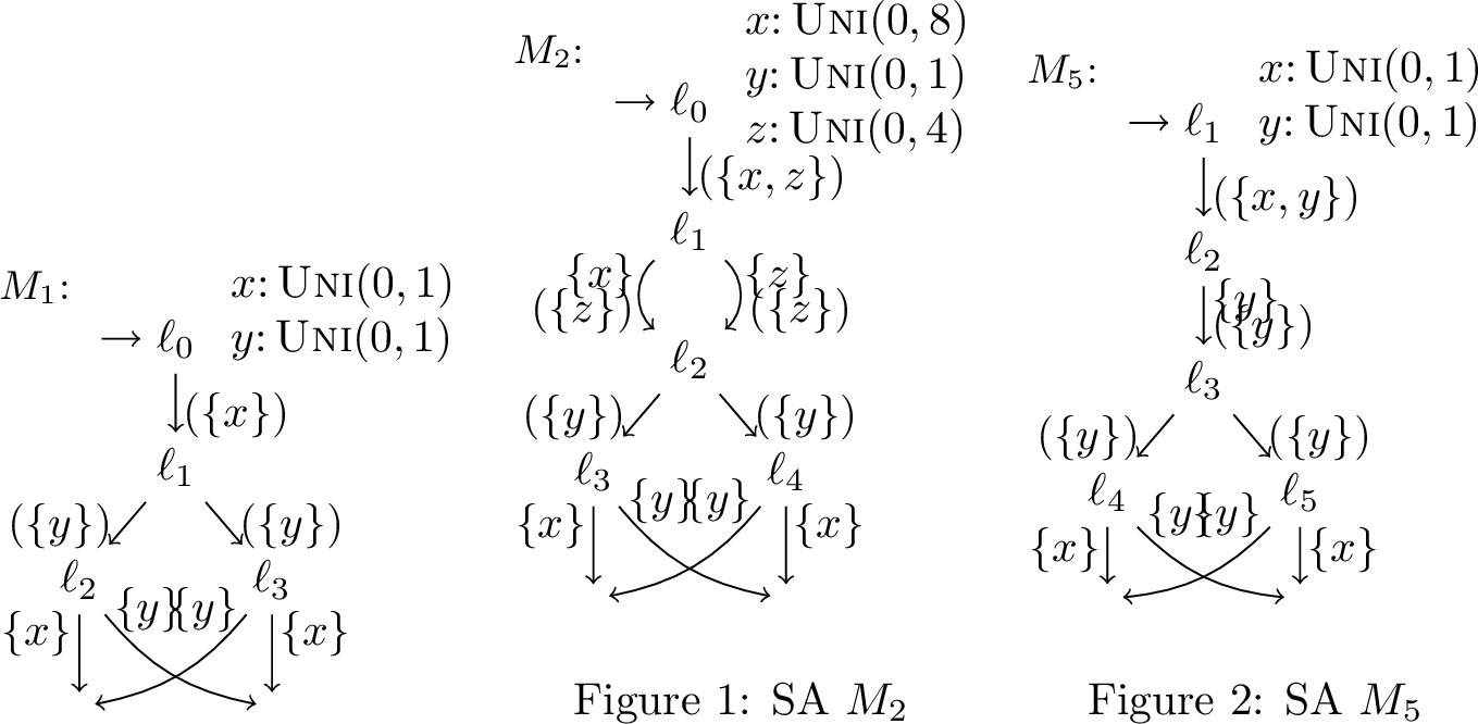
7.1 Exact Probabilities for \(M_1\)↩︎
The exact probabilities for reaching the goal in \(M_1\) are \(p_\mathit{min}= 0.25\) and \(p_\mathit{max}= 0.75\) and can be computed as
\[\begin{align} \textstylep_\mathit{max}&= P(X\leq 0.5) \cdot P(X\leq Y) + P(X\geq 0.5) \cdot P(X\geq Y)\\ &= 0.5\cdot(\int_{0}^{0.5} \int_{x}^{1} f(y) \,dy f(x) \,dx) + 0.5\cdot(\int_{0.5}^{1} \int_{0}^{x} f(y) \,dy f(x)\,dx)\\ &= 0.5 \cdot \int_{0}^{0.5} 2(1-x) \, dx + 0.5\cdot\int_{0.5}^{1} 2x\,dx\\ &= 0.75\\ \end{align}\] and \[\begin{align} \textstylep_\mathit{min}&= P(X\leq 0.5) \cdot P(X\geq Y) + P(X\geq 0.5) \cdot P(X\leq Y)\\ &= 0.5\cdot(\int_{0}^{0.5} \int_{0}^{x} f(y) \,dy f(x) \,dx) + 0.5\cdot(\int_{0.5}^{1} \int_{x}^{1} f(y) \,dy f(x)\,dx)\\ &= 0.5 \cdot \int_{0}^{0.5} 2x \, dx + 0.5\cdot\int_{0.5}^{1} 2(1-x)\,dx\\ &= 0.25. \end{align}\]
The only nondeterministic choice present in \(M_1\) is the choice of the outgoing transition in \(\ell_1\). If the transition to \(\ell_2\) is chosen \(x\) must expire before \(y\) to reach the target state, if the transition to \(\ell_3\) is chosen \(y\) must expire before \(x\) instead. Since \(X,Y \sim Uni(0,1)\) and while the valuation of \(x\) is known in \(\ell_1\), the valuation of \(y\) is resampled on the transitions. Hence, for maximizing the probability of reaching the target location, going to \(\ell_2\) is optimal if \(\vec{x} \leq 0.5\) which is represented by the first integral, where the outer integral for \(x\) ranges from 0 to 0.5 and the inner integral for \(y\) ensures that \(y\) expires after \(x\). In the opposite case where \(\vec{x} \geq 0.5\) going to \(\ell_3\) is optimal, which is accounted for by the second integral.
7.2 Exact Probabilities for \(M_2\)↩︎
\(M_2\) has a similar nondeterministic choice in location \(\ell_2\). However, the valuation of \(x\) in that location depends now also on an additional timer variable \(z\). If initially the sampled valuation \(x\) is lower than the sampled valuation of \(z\), the transition to \(\ell_2\) guarded by \(x\) is taken, meaning that \(x = \lightning\) in \(\ell_2\) and thus allowing optimal decisions. In the opposite case where initially \(\vec{x} > \vec{z}\) the optimal choice depends on the remaining valuation of \(x\) in location \(\ell_2\). The CPD for that can be computed as \(C=X-Z\).
7.2.1 CDF of \(C = X - Z\).↩︎
Since \(X \sim \mathrm{Uniform}[0,8]\) and \(Y \sim \mathrm{Uniform}[0,4]\), so their PDFs are \[f_X(x) = \frac{1}{8} \quad (x \in [0,8]), \qquad f_Y(y) = \frac{1}{4} \quad (y \in [0,4]).\] The difference \(Z = X - Y\) ranges over \([-4,\, 8]\). The combined PDF \(f_Z(z)\) can be obtained using convolution
\[f_Z(z) = \int_{-\infty}^{\infty} f_X(t)\, f_Y(t - z)\, dt = \int_{-\infty}^{\infty} \frac{1}{8} \cdot \frac{1}{4} \cdot \mathbf{1}[t \in [0,8]] \cdot \mathbf{1}[t - z \in [0,4]]\, dt.\]
The second indicator requires \(t \in [z,\, z + 4]\), so the effective integration range is \(t \in [\max(0,\, z),\, \min(8,\, z+4)]\), and the integrand equals \(\tfrac{1}{32}\) throughout. This interval changes across three cases.
Case 1: \(-4 \leq z < 0\). Both constraints give \(t \geq 0\) and \(t \leq z + 4\). Since \(z + 4 < 4 \leq 8\) we have \(\min(8,\, z+4) = z + 4\), so the length is \((z+4) - 0 = z + 4\): \[f_Z(z) = \frac{1}{32}(z + 4).\]
Case 2: \(0 \leq z \leq 4\). Lower bound: \(\max(0,z) = z\). Upper bound: \(\min(8,\, z+4) = z+4\) (since \(z + 4 \leq 8\)). Length \(= 4\): \[f_Z(z) = \frac{4}{32} = \frac{1}{8}.\]
Case 3: \(4 < z \leq 8\). Lower bound: \(\max(0,z) = z\). Upper bound: \(\min(8,\, z+4) = 8\) (since \(z + 4 > 8\)). Length \(= 8 - z\): \[f_Z(z) = \frac{1}{32}(8 - z).\]
Combining all three cases gives the full PDF: \[\boxed{f_Z(z) = \begin{cases} \dfrac{z+4}{32} & -4 \leq z < 0, \\[8pt] \dfrac{1}{8} & 0 \leq z \leq 4, \\[8pt] \dfrac{8-z}{32} & 4 < z \leq 8. \end{cases}}\]
Using the combined probability distribution for \(C = X -Z\) the exact maximal reachability probability can be computed as: \[\begin{align} \textstylep_\mathit{max}&= P(X-Z \leq 0) + P(X-Z \leq 0.5 \wedge X-Z \leq Y)\\&\phantom{=}\;+ P(X-Z \geq 0.5 \wedge X-Z \geq Y)\\ &= \int_{-4}^{0} \frac{1}{32} (c + 4) \,dc + \int_{0}^{0.5} \int_{c}^{1} f_C(c) f_Y(y) \,dc \,dy \\&\phantom{=}\;+ \int_{0.5}^{8} \int_{0}^{c} f_C(c) f_Y(y) \,dc \,dy\\ &= \int_{-4}^{0} \frac{1}{32} (c + 4) \,dc + \int_{0}^{0.5} \int_{c}^{1} f_C(c) f_Y(y) \,dc \,dy\\&\phantom{=}\;+ \int_{0.5}^{1} \int_{0}^{c} f_C(c) f_Y(y) \,dc \,dy + \int_{1}^{8} f_C(c)\,dc \\ &= \int_{-4}^{0} \frac{1}{32} (c + 4) \,dc + \int_{0}^{0.5} \int_{c}^{1} \frac{1}{8} \cdot 1 \,dc \,dy\\&\phantom{=}\;+ \int_{0.5}^{1} \int_{0}^{c} \frac{1}{8} \cdot 1 \,dc \,dy + \int_{1}^{4} f_C(c)\,dc + \int_{4}^{8} f_C(c)\,dc\\ &= \int_{-4}^{0} \frac{1}{32} (c + 4) \,dc + \int_{0}^{0.5} \frac{1}{8} (1-c) \,dc\\&\phantom{=}\;+ \int_{0.5}^{1} \frac{1}{8} c \,dc + \int_{1}^{4} f_C(c)\,dc + \int_{4}^{8} f_C(c)\,dc\\ &= \frac{1}{32} \left[0.5c^2 + 4c \right]_{-4}^{0} + \left[\frac{1}{8}c - \frac{1}{8} \cdot \frac{1}{2} c^2 \right]_{0}^{0.5} + \left[ \frac{1}{16} c^2 \right]_{0.5}^{1}\\&\phantom{=}\;+ \left[ \frac{1}{8} c \right]_{1}^{4} + \frac{1}{32}\left[ 8 c - \frac{1}{2} c^2\right]_{4}^{8}\\ &= \frac{1}{4} + (\frac{1}{8}(\frac{1}{2} - \frac{1}{8}) + (\frac{1}{16} - \frac{1}{16} \cdot \frac{1}{4}) + (\frac{4}{8} - \frac{1}{8}) + \frac{1}{32}\left( \frac{64}{2} - 24 \right)\\ &= \frac{1}{4} + \frac{1}{8} \cdot\frac{3}{8} + \frac{3}{64} + \frac{3}{8} + \frac{8}{32}\\ &= \frac{31}{32} = 0.96875\\ \end{align}\]
and, since for \(C < 0\) and \(C >1\) an optimal decision which avoids the target state is possible,
\[\begin{align} \textstylep_\mathit{min}&= P(0 \leq C \leq 0.5 \wedge Y \leq C) + P(0.5 \leq C \leq 1 \wedge Y \geq C)\\ &= \int_{0}^{0.5} \int_{0}^{c} f_C(c) \,dc f_Y(y) \,dy + \int_{0.5}^{1} \int_{c}^{1} f_C(c) \,dc f_Y(y) \,dy\\ &= \int_{0}^{0.5} \frac{1}{8} c \,dc + \int_{0.5}^{1} \frac{1}{8} (1-c) \,dc \\ &= \left[ \frac{1}{16} c^2 \right]_{0}^{0.5} + \frac{1}{8} \left[c - 0.5 c^2 \right]_{0.5}^{1} \\ &= \frac{1}{16} \cdot \frac{1}{4} + \frac{1}{8} (1 - \frac{1}{2} - (\frac{1}{2} - \frac{1}{8}))\\ &= \frac{1}{16} \cdot \frac{1}{4} + \frac{1}{8} (\frac{1}{8})\\ &= \frac{1}{32} = 0.03123\\. \end{align}\]
7.3 Exact Probabilities for \(M_5\)↩︎
For \(M_5\) the optimal probabilities to reach or avoid the target state are determined by the nondeterministic choice in location \(\ell_3\). If initially the sampled valuation for \(x\) is below the sampled valuation of \(y\), then x is already expired in \(\ell_3\). Since both both timers are uniformly distributed on \((0,1)\) the probability that is \(P(X \leq Y) = 0.5\) and in that case \(x= \lightning\) means that the reset value of \(y\) does not influence the result. In the opposite case where initially \(\vec{v} > \vec{y}\) the optimal choice in Location \(\ell_3\) depends on the remaining valuation of \(x\). The optimal decisions are similarly to \(M_1\): if \(\vec{x} \leq 0.5\) the optimal choice for maximal winning chances is taking the transition to Location \(\ell_4\) and if \(v(x) \geq 0.5\) it is the transition to \(\ell_5\). The remaining valuation of \(x\) can be computed as the joint probability function \(Z = X-Y\) .
7.3.1 PDF of \(Z = X - Y\)↩︎
Since \(X, Y \sim Uni(0,1)\) independently, \(Z\) ranges over \([-1, 1]\). Using convolution, the probability density function of \(Z\) is: \[f_Z(z) = \int_{-\infty}^{\infty} f_X(t)\, f_Y(t - z)\, dt.\] Both densities equal \(1\) on \([0,1]\) and \(0\) elsewhere, so the integrand is \(1\) only when \(t \in [0,1]\) and \(t - z \in [0,1]\), i.e.\(t \in [\max(0,z),\, \min(1, 1+z)]\).
Case 1: \(0 \leq z \leq 1\). \[f_Z(z) = \int_z^1 dt = 1 - z.\]
Case 2: \(-1 \leq z < 0\). \[f_Z(z) = \int_0^{1+z} dt = 1 + z.\]
Hence the full PDF is: \[\boxed{f_Z(z) = 1 - |z|, \qquad z \in [-1,\, 1].}\] This is the symmetric triangular distribution on \([-1, 1]\), with the peak at \(z = 0\). The exact probabilities for reaching the goal in \(M_5\) are \(p_\mathit{min}= 0.125\) and \(p_\mathit{max}= 0.875\) and can be computed as
\[\begin{align} p_{\max} &= P(X \leq Y_0) + P(0\leq X-Y_0 \leq 0.5) + P(X-Y_0 \geq 0.5)\\ &= 0.5 + 0.5\cdot\left(\int_{0}^{0.5} \int_{z}^{1} f_z(z) \,dz\, f_y(y) \,dy\right) + 0.5\cdot\left(\int_{0.5}^{1} \int_{0}^{z} f_z(z) \,dz\, f_y(y)\,dy\right) \\ &= 0.5 + 0.5\cdot\left(\int_{0}^{0.5} f_z(z)(1-z) \,dz\right) + 0.5\cdot\left(\int_{0.5}^{1} f_z(z)\,z \,dz\right) \\ &= 0.5 + 0.5\cdot\left(\int_{0}^{0.5} (1-z)^2 \,dz\right) + 0.5\cdot\left(\int_{0.5}^{1} z(1-z) \,dz\right) \\ &= 0.5 + \left[z - z^2 + \frac{1}{3}z^3\right]_{0}^{0.5} + \left[\frac{1}{2}z^2 - \frac{1}{3}z^3\right]_{0.5}^{1} \\ &= 0.5 + \left(0.5 - 0.25 + \frac{1}{3}\cdot\frac{1}{8}\right) - 0 + \left(\frac{1}{2} - \frac{1}{3}\right) - \left(\frac{1}{8} - \frac{1}{3}\cdot\frac{1}{8}\right) \\ &= 0.875 \end{align}\] and \[\begin{align} p_{\min} &= 0.5\cdot\left(\int_{0}^{0.5} \int_{0}^{z} f_z(z) \,dz\, f_y(y) \,dy\right) + 0.5\cdot\left(\int_{0.5}^{1} \int_{z}^{1} f_z(z) \,dz\, f_y(y)\,dy\right) \\ &= 0.5\cdot\left(\int_{0}^{0.5} f_z(z)z \,dz\right) + 0.5\cdot\left(\int_{0.5}^{1} f_z(z)(1-z) \,dz\right) \\ &= 0.5\cdot\left(\int_{0}^{0.5} (1-z)z \,dz\right) + 0.5\cdot\left(\int_{0.5}^{1} (1-z)^2 \,dz\right) \\ &= \left[\frac{1}{2}z^2 - \frac{1}{3}z^3 \right]_{0}^{0.5} + \left[ z - z^2 + \frac{1}{3}z^3 \right]_{0.5}^{1} \\ &= \frac{1}{8} - \frac{1}{3}\cdot\frac{1}{8} - 0 + 1 -1 + \frac{1}{3} -\left(\frac{1}{2} - \frac{1}{2} + \frac{1}{3}\cdot\frac{1}{8}\right) \\ &= 0.125 \end{align}\]
References↩︎
Authors are sorted in alphabetical order. This work was supported by the EU’s H2020 R & I programme under MSCA grant agreement 101008233 (MISSION), by the Interreg North Sea project STORM_SAFE, by SeCyT-UNC grant 33620230100384CB (MECANO), and by NWO VIDI grant VI.Vidi.223.110 (TruSTy).↩︎
Two timers expiring simultaneously has probability \(0\) because of our restriction to absolutely continuous distributions, so we can disregard this case here.↩︎
Consider tossing a coin to then nondeterminstically guess its value vs.the inverse.↩︎