1 Introduction↩︎

Which voting rules are more resilient to coalitional manipulation? This question has long motivated research in social choice theory, yet remains difficult to answer in general terms. The Gibbard–Satterthwaite theorem establishes that no non-trivial voting rule can be entirely immune to manipulation, but it leaves open the possibility of meaningful comparisons between rules. This paper develops a principled framework for such comparisons, based on a deliberately simple probabilistic model that captures the essential structure of voting rule vulnerability.

1.1 Motivation↩︎

A voting rule is coalitionally manipulable (CM) in a given profile if a subset of voters could obtain a preferred outcome by misreporting their preferences. This property can be interpreted ex ante as a vulnerability to strategic voting, or ex post as a source of regret for sincere voters, potentially undermining trust in electoral outcomes [1], [2]. While the Gibbard–Satterthwaite theorem implies that any non-trivial voting rule is susceptible to this phenomenon [3], [4], it remains possible to compare the vulnerability of voting rules, in particular through their CM rate, defined as the theoretical or empirical proportion of profiles in which the rule is coalitionally manipulable.

To explain the low empirical vulnerability of Instant-Runoff Voting (IRV), [5] relies on the Perturbed Culture model introduced by [6], in which one ranking is favored by a concentration parameter \(\theta\) while all others are equally probable. Comparing IRV with Plurality and Plurality with Runoff, this study identifies a phase transition characterized by a critical concentration parameter \(\theta_c(f,m)\), depending on the voting rule \(f\) and the number of candidates \(m\). In the subcritical regime \(\theta<\theta_c(f,m)\), the CM rate converges to \(1\) for large electorates, whereas in the supercritical regime \(\theta>\theta_c(f,m)\) it converges to \(0\). The parameter \(\theta_c(f,m)\) thus measures how quickly a rule becomes resistant to coalitional manipulation as preference concentration increases. For IRV and its variants, the introduction of the Super Condorcet Winner (SCW) yields \(\theta_c(f,m)=0\), showing resilience even under arbitrarily small preference concentration.

The goal of the present study is to determine whether the Perturbed Culture model can also shed light on the comparative performance of different voting rules. While IRV is particularly resilient, one may wish to use alternative rules that satisfy axiomatic properties violated by IRV, such as monotonicity. This raises a natural question: among standard voting rules satisfying certain axiomatic properties, which ones should be preferred in order to minimize vulnerability to coalitional manipulation? Our objective is to provide a principled way to rank voting rules with respect to this criterion, thereby addressing this question beyond the special case of IRV.

Rather than aiming for a realistic model fitted to empirical data through multiple parameters, we deliberately focus on a minimal model. The ability of such a simple framework to reproduce observed qualitative phenomena provides evidence that it captures key underlying mechanisms.

1.2 Contributions↩︎

This paper makes three main contributions.

1.2.0.1 Theoretical framework

We substantially extend the work of [5] through a systematic analysis of all standard ordinal voting rules. We introduce two strengthened notions of Condorcet winners:

• The Pair-Safe Condorcet Winner, characterizing Maximin, Ranked Pairs, Schulze, and Young;

• The Set-Safe Condorcet Winner, characterizing Baldwin, Nanson, Kemeny, and Simplified Dodgson.

Together with the existing notion of Resistant Condorcet Winner [7], which we show underlies the behavior of Black, Slater, and Copeland, these notions form a natural hierarchy, while the remaining voting rules are analyzed on a case-by-case basis. For each rule, we establish the existence of a phase transition and determine the critical concentration parameter \(\theta_c(f, m)\).

1.2.0.2 Empirical validation

We test our theoretical predictions on the Netflix and FairVote datasets using an enhanced version of the SVVAMP package [8], [9]. Our contributions include five new voting rules (Kemeny, Slater, Young, Dodgson, and Simplified Dodgson) and improved manipulation algorithms for five others (Ranked Pairs, Baldwin, Nanson, Copeland, and Kim–Roush). The key empirical findings are:

• Rules belonging to the same theoretical family exhibit strikingly similar CM rates;

• The theoretical bounds from our Condorcet notions are almost tight in practice;

• The model accurately predicts the relative ranking of voting rules by vulnerability, largely independent of the dataset.

1.2.0.3 Predictive power without fitting

The model uses no tunable parameters beyond the number of candidates \(m\), yet it accurately predicts the relative vulnerability of voting rules across datasets with very different absolute CM rates.

1.3 Related Work↩︎

Several studies analyze coalitional manipulability from a theoretical perspective [10]–[13]. In particular, [14] show that many rules have a limiting CM rate equal to \(1\) under Impartial Culture, which prevents this criterion from meaningfully discriminating between them.

[15] identifies a form of phase transition for coalitional manipulation phenomena. In that work, this transition is studied with respect to a budget \(B\) for the number of manipulators, whereas our analysis focuses on the concentration of voters’ preferences. Moreover, for many standard voting rules, it is shown that in Impartial Culture, the CM rate with \(n\) voters and budget \(B\) is \(\Theta(\min\{ \frac{B}{\sqrt{n}}, 1 \})\). While this result provides valuable insight into the role of the number of manipulators, it cannot be used to compare voting rules.

Empirically, several studies have compared CM rates across voting rules [16]–[19]. Analyses based on both artificial cultures and real-world datasets [2], [20] have highlighted similarities in behavior among rules such as Maximin, Ranked Pairs, and Schulze. We extend these results by identifying additional families of voting rules, first at the theoretical level and then empirically, thanks to the implementation of more precise manipulation algorithms.

Finally, a large body of work studies the algorithmic complexity of individual or coalitional manipulation, which we do not address here (see [21] for an overview).

1.4 Limitations↩︎

This study has two main limitations. First, it excludes non-ordinal rules such as Approval, Range Voting, Majority Judgment, or STAR. Second, while the model accurately captures the behavior of most rules, it does not explain the near-identical empirical CM rates of Kim–Roush and Veto, and its predictions are less precise for Bucklin and Coombs (see Section 4.2).

1.5 Roadmap↩︎

Section 2 introduces the framework and notation. Section 3 presents the theoretical results, and Section 4 reports the numerical experiments. Section 5 concludes with perspectives for future work.

2 Framework↩︎

This section introduces the framework and notation used throughout the paper. Section 2.1 recalls standard notions from voting theory and defines the Perturbed Culture model used in this work. Section 2.2 reviews the voting rules considered. Finally, Section 2.3 summarizes the main results established by [5], which serve as a starting point for our analysis.

2.1 Voting Theory and Model↩︎

We introduce the basic notions of voting theory and the probabilistic model considered in this work. Our notation mostly follows that of [5].

A discrete profile \(P\) consists of a finite, non-empty set of candidates \(\mathcal{C}(P)\), with \(m(P)=|\mathcal{C}(P)|\); a finite, non-empty set of voters \(\mathcal{V}(P)\), with \(n(P)=|\mathcal{V}(P)|\); and, for each voter \(v \in \mathcal{V}(P)\), a preference ranking \(P_v\) over \(\mathcal{C}(P)\). For a ranking \(r\), let \(w(r,P)\) denote its weight, that is, the number of voters whose preference ranking is \(r\). The total weight of \(P\) is then \(w(P)=\sum_r w(r,P)=n(P)\).

A continuous profile \(P\) consists of a finite, non-empty set of candidates \(\mathcal{C}(P)\), with \(m(P)=|\mathcal{C}(P)|\); a total weight \(w(P)\in(0,\infty)\); and, for each ranking \(r\) over \(\mathcal{C}(P)\), a weight \(w(r,P)\in[0,\infty)\), satisfying \(\sum_r w(r,P)=w(P)\).

For any profile \(P\), discrete or continuous, the normalized profile \(\bar{P}\) is the continuous profile defined by \(w(r,\bar{P}) = \frac{w(r,P)}{w(P)}.\)

We use the following notation for restricted profiles. For \(K \subseteq \mathcal{C}(P)\), let \(P_{K}\) denote the restriction of \(P\) to the candidates in \(K\). For a candidate \(c\) and a position \(k\), let \(P^{r(c)=k}\) (resp.\(P^{r(c)\leq k}\)) denote the sub-profile of voters ranking \(c\) in position \(k\) (resp.among their top \(k\) positions). For \(c,d \in \mathcal{C}(P)\), let \(P^{c \succ d}\) denote the restriction of \(P\) to voters preferring \(c\) to \(d\), and similarly for multiple comparisons (e.g., \(P^{c \succ d \text{ and } c \succ e}\)). These notations can be combined to restrict simultaneously to a subset of candidates and a subset of voters.

A voting rule \(f\) maps any discrete profile \(P\) to a candidate in \(\mathcal{C}(P)\). Almost all rules considered here extend naturally to continuous profiles and are homogeneous, in the sense that their outcome \(f(P)\) depends only on the normalized profile \(\bar{P}\). The only exceptions are Young, Dodgson, and Simplified Dodgson (see Section 2.2.2).

For candidates \(c,d \in \mathcal{C}(P)\), let \(W(c,d,P)=w(P^{c \succ d})\) denote the total weight of voters preferring \(c\) to \(d\) in profile \(P\). The matrix \(W(P)\) with entries \(W(c,d,P)\) is the weighted majority matrix of \(P\). The unweighted majority matrix \(M(P)\) is obtained from \(W(P)\) by setting \(M(c,d,P)\) equal to \(1\) (resp.\(\tfrac{1}{2}\), \(0\)) if \(W(c,d,P)\) is greater than (resp.equal to, less than) \(W(d,c,P)\); by convention, diagonal entries are set to \(0\). A candidate \(c\) is the Condorcet winner of a profile \(P\) if \(M(c,d,P)=1\) for every other candidate \(d\). A voting rule \(f\) is Condorcet-consistent if it elects the Condorcet winner whenever one exists. The Smith set of a profile \(P\) is the smallest non-empty subset \(K \subseteq \mathcal{C}(P)\) such that \(M(c,d,P)=1\) for all \(c \in K\) and \(d \in \mathcal{C}(P)\setminus K\). In particular, if a Condorcet winner exists, it is the unique member of the Smith set.

For a discrete profile \(P\), we say that a voting rule \(f\) is coalitionally manipulable (CM) in \(P\) (or that \(P\) is CM in \(f\)) if there exists a target profile \(Q\) with the same candidates and voters such that \(f(Q)\neq f(P)\), and every voter who changes their ballot prefers \(f(Q)\) to \(f(P)\) according to their true ranking \(P_v\). For a continuous profile \(P\), assuming that \(f\) is defined on continuous profiles, we say that \(f\) is coalitionally manipulable (CM) in \(P\) if there exists a target profile \(Q\) with the same candidates and total weight such that \(f(Q)\neq f(P)\), and for every ranking \(r\), whenever \(w(r,Q)<w(r,P)\) the ranking \(r\) places \(f(Q)\) above \(f(P)\). Throughout the paper, we use the terms “coalitionally manipulable” (CM) and “susceptible to coalitional manipulation” interchangeably. Likewise, we use “non-coalitionally manipulable” (non-CM) interchangeably with “immune to coalitional manipulation”.

We now introduce the probabilistic model and the quantitative measure of coalitional manipulability central to our analysis, following [5].

Given integers \(n,m>0\) and a concentration parameter \(\theta\in(0,1]\), the Perturbed Culture generates a random discrete profile \(P\) with \(\mathcal{C}(P)=\{1,\ldots,m\}\) and \(\mathcal{V}(P)=\{1,\ldots,n\}\). Each voter independently adopts the reference ranking \((1,\ldots,m)\) with probability \(\theta\), and a uniformly random ranking otherwise. We exclude the case \(\theta=0\), which corresponds to the classical model of Impartial Culture.

We denote by \(\hat{P}\) the expected normalized profile, or simply the expected profile, defined as the continuous profile in which each ranking has weight \(\tfrac{1-\theta}{m!}\), except for the reference ranking \((1,\ldots,m)\), which has weight \(\theta+\tfrac{1-\theta}{m!}\). For concision, we leave the dependence of \(\hat{P}\) on \(\theta\) and \(m\) implicit. The expected profile \(\hat{P}\) serves as the asymptotic limit of normalized profiles as the number of voters grows, and plays a central role in the proofs.

For a dataset of profiles, the CM rate of a voting rule \(f\) is the fraction of profiles that are CM in \(f\); for a probabilistic model, it is the probability that a random profile is CM. We write \(\rho(f,m,n,\theta)\) for the CM rate of \(f\) in the Perturbed Culture with parameters \(m,n,\theta\).

2.2 Voting Rules↩︎

We now review the voting rules considered in this paper. To keep the presentation concise, rules are grouped into broad categories, although many could naturally belong to more than one. All rules are assumed to use a tie-breaking mechanism; unless otherwise specified (Slater and Copeland), our theoretical results do not depend on it, and numerical simulations break ties in favor of candidates with smaller indices. Readers familiar with standard voting rules may safely jump directly to Section 2.3. Some additional voting rules are considered in the technical appendix.

2.2.1 Score-based rules↩︎

Elect the candidate \(c\) with maximal score \(s_f(c, P)\).

Plurality (Plu). \(s_\textrm{Plu}(c, P) = w(P^{r(c) = 1})\).

Borda (Bor). \(s_\textrm{Bor}(c, P) = \sum_{k=1}^{m(P)} (m(P) - k)\,w(P^{r(c) = k})\).

Veto (Vet). \(s_\textrm{Vet}(c, P) = -\,w(P^{r(c) = m(P)})\).

Maximin (Max). \(s_\textrm{Max}(c, P) = \min_{d \in \mathcal{C}(P) \setminus \{c\}} W(c, d, P)\).

Copeland (Cop). \(s_\textrm{Cop}(c,P)=|\{d\in\mathcal{C}(P):M(c,d,P)=1\}| + \alpha\,|\{d\in\mathcal{C}(P)\setminus\{c\}:M(c,d,P)=\tfrac{1}{2}\}|\), with \(\alpha\in[0,1]\). Our theoretical results in the main body do not depend on \(\alpha\); in simulations, we set \(\alpha=\tfrac{1}{2}\).

Bucklin (Buc). \(s_\textrm{Buc}(c,P) = (-\mu(c,P),\, w(P^{r(c)\leq \mu(c,P)}))\), where \(\mu(c,P)\) is the median rank of \(c\). Scores are compared lexicographically.

2.2.2 Penalty-based rules (candidate level)↩︎

Elect the candidate \(c\) with minimal penalty \(p_f(c,P)\).

Young (You). \(p_\textrm{You}(c,P)\) is the minimal number of voters to remove so that \(c\) becomes the Condorcet winner. If this is impossible, \(p_\textrm{You}(c,P)=n(P)+1\).

Dodgson (Dod). \(p_\textrm{Dod}(c,P)\) is the minimal number of adjacent swaps in voters’ rankings required to make \(c\) the Condorcet winner.

Simplified Dodgson (SD). \(p_\textrm{SD}(c,P)=\sum_{d\in\mathcal{C}(P)\setminus\{c\}}\max(0, \lfloor\tfrac{n(P)}{2}\rfloor+1-W(c,d,P))\). This corresponds to the minimal number of pairwise comparisons by individual voters that must be changed for \(c\) to become a Condorcet winner, without requiring ballots to remain transitive as in the Dodgson rule.¹ We include this rule mainly to provide insight into the behavior of the Dodgson rule (Section 3.2).

2.2.3 Penalty-based rules (ranking level)↩︎

Find a ranking with minimal penalty \(p_f(r,P)\), and elect its top candidate.

Kemeny (Kem). \(p_\textrm{Kem}(r,P)=\sum_{(c,d)\in\mathcal{C}(P)^2:\,c\succ_r d}W(d,c,P)\).

Slater (Sla). \(p_\textrm{Sla}(r,P)=\sum_{(c,d)\in\mathcal{C}(P)^2:\,c\succ_r d}M(d,c,P)\).

2.2.4 Elimination rules↩︎

Eliminate one or more candidates in successive rounds until a single winner remains.

IRV, Baldwin, Coombs (IRV, Bal, Coo). Iteratively eliminate the candidate with the lowest plurality, Borda, or veto score, respectively.

Nanson, Kim–Roush (Nan, KR). At each round, eliminate all candidates whose Borda or veto score is below the average, respectively.²³

Plurality with runoff (PR). Keep the top two candidates by plurality, then elect the one winning their pairwise contest.

2.2.5 Other Condorcet rules↩︎

This last category gathers standard Condorcet-consistent rules, complementing those already mentioned: Maximin, Copeland, Young, Dodgson, Kemeny, and Slater.

Black (Bla). Elect the Condorcet winner if one exists; otherwise elect the Borda winner.

Ranked Pairs (RP). Order all pairs of candidates by decreasing \(W(c,d,P)\). Iteratively lock each pair into a directed graph unless this creates a cycle. Elect the unique source of the final graph [24].

Schulze (Sch). Define the strength of \(c\) over \(d\) as the width of the widest path from \(c\) to \(d\) in the weighted majority graph induced by \(W(P)\): \[\textrm{Strength}(c,d,P) = \max_{\text{paths p from c to d}} \;\min_{(i,j)\in p} W(i,j,P).\] Elect a candidate \(c\) such that \(\textrm{Strength}(c,d,P) \geq \textrm{Strength}(d,c,P)\) for all \(d\) [25].

2.3 Known Results: Phase Transitions in the Perturbed Culture↩︎

The Perturbed Culture model was introduced by [6] as a conceptual tool to assess the practical relevance of the Condorcet paradox. Under Impartial Culture, the probability that no Condorcet winner exists converges to a positive limit as the electorate grows, suggesting a non-negligible prevalence of this phenomenon in practice. By contrast, under the Perturbed Culture, as soon as the concentration parameter \(\theta\) is strictly positive, however small, this probability converges to \(0\), indicating that the Condorcet paradox may be exceptional. Although both models are highly stylized and make no claim of realism, this latter prediction turns out to be more consistent with empirical observations, as Condorcet winners are extremely frequent in real-world datasets [17], [20].

[5] uses the Perturbed Culture model to study coalitional manipulability for three voting rules: Plurality, Plurality with Runoff, and IRV. In the case of Plurality, for \(m\geq 2\), it is shown that there exists a critical concentration parameter \(\theta_c(\textrm{Plu},m)=\frac{m-2}{3m-2}\) such that

• if \(\theta<\theta_c(\textrm{Plu},m)\), then \(\lim_{n\to\infty}\rho(\textrm{Plu},m,n,\theta)=1\);

• if \(\theta>\theta_c(\textrm{Plu},m)\), then \(\lim_{n\to\infty}\rho(\textrm{Plu},m,n,\theta)=0\).

This result exhibits a phase transition, that is, an abrupt change in the asymptotic behavior of the CM rate when the concentration parameter \(\theta\) crosses the critical threshold. This phenomenon is illustrated in Figure 1, which displays the CM rate of Plurality as a function of \(\theta\) for increasing values of \(n\). As \(n\) grows, the curve takes on a sigmoidal shape and converges to a step function. Moreover, the convergence is shown to be exponentially fast, implying that the asymptotic behavior predicted by the theorem quickly becomes relevant as the electorate grows. For Plurality with Runoff, similar results hold, but with a smaller critical parameter, \(\theta_c(\textrm{PR},m)=\frac{m-3}{5m-3}\) for \(m\geq 3\).

To address the case of IRV, [5] introduces the notion of a Super Condorcet Winner (SCW), defined as a candidate \(c\) such that, for every subset \(K\subseteq\mathcal{C}(P)\) containing \(c\) with \(|K|\geq 2\), \[\label{eq:def95scw} s_\textrm{Plu}(c,P_K)>\frac{w(P)}{|K|},\tag{1}\] that is, \(c\) has a plurality score strictly above average in all these restricted profiles. Whenever such a candidate exists, it is elected by IRV and the profile is immune to coalitional manipulation. As in the case of Condorcet winners, for any concentration parameter \(\theta>0\), an SCW exists with high probability, namely with probability tending to \(1\) as the electorate grows, implying that IRV is immune to coalitional manipulation. As a consequence, the critical concentration parameter for IRV is \(\theta_c(\textrm{IRV},m)=0\). Moreover, although the existence of an SCW is only a sufficient condition, it is also observed in empirical datasets that it explains most cases in which IRV is immune to coalitional manipulation.

In all cases, the proof strategy follows the same general pattern. One first analyzes the expected profile, which is susceptible to coalitional manipulation when the concentration parameter \(\theta\) is small enough and immune to coalitional manipulation otherwise. This property is then shown to be stable in a neighborhood of the expected profile, with technical subtleties arising in some cases from the need to control stability both around the sincere profile and around potential manipulated profiles. Finally, the result is extended to discrete profiles in the limit \(n\to\infty\) using the weak law of large numbers. Altogether, this approach shows that a simple and mathematically tractable model suffices to explain qualitative phenomena such as the low vulnerability of IRV observed in empirical data.

The paper also shows that a deliberately constructed voting rule may fail to exhibit a phase transition with a well-defined critical concentration parameter \(\theta_c(f,m)\). Nevertheless, it is always possible to define a lower critical concentration parameter \(\theta_{\ell}(f,m) \in [0, 1]\) and an upper critical concentration parameter \(\theta_u(f,m) \in [0, 1]\) as the largest and smallest values, respectively, such that the following holds for every \(\theta \in (0, 1]\):

• if \(\theta<\theta_\ell(f,m)\), then \(\lim_{n\to\infty}\rho(f,m,n,\theta)=1\);

• if \(\theta>\theta_u(f,m)\), then \(\lim_{n\to\infty}\rho(f,m,n,\theta)=0\).

The critical concentration parameter \(\theta_c(f, m)\) is then simply defined as their common value when it exists.

3 Theoretical Results↩︎

[5] established the existence of a phase transition for three voting rules, while observing that one can deliberately construct exotic voting rules to serve as counterexamples. From a theoretical perspective, our main objective is to continue this research program by establishing the existence of a phase transition for each voting rule studied in this paper, and by identifying the corresponding critical concentration parameter.

In the same spirit as the IRV analysis based on the Super Condorcet Winner (SCW), we rely on several strengthened notions of the Condorcet winner to capture the behavior of other rules. We introduce the Pair-Safe Condorcet Winner (PSCW) in Section 3.1 to analyze Maximin, Ranked Pairs, Schulze, and Young. We then define the Set-Safe Condorcet Winner (SSCW) in Section 3.2 for Baldwin, Nanson, Kemeny, and Simplified Dodgson. In Section 3.3, we rely on the existing notion of a Resistant Condorcet Winner (RCW) [7] to study Black, Slater, and Copeland. These notions form a hierarchy of implications: \[\text{RCW} \;\Rightarrow\; \text{SSCW} \;\Rightarrow\; \text{PSCW} \;\Rightarrow\; \text{CW},\] whereas the Super Condorcet Winner (SCW) only implies CW and is logically independent of the others. When dealing with a Condorcet notion, we will also use the notation \(\theta_c(\cdot, m)\) to denote the critical concentration parameter above which such a winner exists with high probability, and below which it does not. For example, \(\theta_c(\textrm{SCW}, m) = 0\).

Finally, in Section 3.4, we briefly discuss the remaining rules and present our main theorem, which shows that every voting rule considered in this paper undergoes a phase transition and characterizes the associated critical concentration parameter.

For the sake of clarity and concision, some proofs are deferred to the technical appendix.

3.1 Pair-Safe Condorcet Winner (PSCW)↩︎

To build intuition, we start with Maximin. Let \(c\) be the winner, and consider a manipulation attempt in favor of some candidate \(d\). Manipulators cannot increase the pairwise score of \(d\) against \(c\), which is \(w(P^{d \succ c})\). Therefore, for the manipulation to succeed, they must reduce the score of \(c\) against some candidate \(e\) to at most this value. Note that if \(c\) is not a Condorcet winner, then candidate \(e\) may coincide with \(d\); otherwise, \(e\) must be a third candidate. In the extreme case where all manipulators rank \(e\) above \(c\), the score of \(c\) against \(e\) drops to \(w(P^{c \succ d \text{ and } c \succ e})\), which comes only from sincere voters preferring \(c\) to \(e\). Manipulation therefore requires \(w(P^{c \succ d \text{ and } c \succ e}) \leq w(P^{d \succ c}).\) The negation of this inequality yields a sufficient condition under which Maximin is immune to coalitional manipulation, motivating the following definition.

Taking \(d=e\) in Equation ?? shows that every PSCW is a Condorcet winner. The converse does not hold: a candidate may be a Condorcet winner without being a PSCW, as illustrated in Table ¿tbl:tab:ex_scw_no_pscw_rules_not_CM?. This profile will be reused throughout the paper; the technical appendix collects the claims it supports for easy reference.

\(\begin{array}{ccc} \hline 5 & 4 & 2 \\ \hline B & A & C \\ A & C & A \\ C & B & B \\ \hline \end{array}\)

To extend our analysis beyond Maximin, we introduce the notion of a Maximin-like voting rule, which clearly includes Ranked Pairs and Schulze.

By the same reasoning as for Maximin, we obtain the following result.

Young fits into this picture as a particular case.

The first statement is illustrated by Table ¿tbl:tab:ex_you_is_not_maximin_like?, while the second relies on more subtle arguments and is proved in Appendix 8.1.2.

\(\begin{array}{c c c} \hline 30 & 72 & 72 \\ \hline A & C_\bullet & B \\ B & C_\bullet & C_\bullet \\ C_\bullet & A & C_\bullet \\ C_\bullet & B & A \\ C_\bullet & C_\bullet & C_\bullet \\ \hline \end{array}\)

For Maximin, Ranked Pairs, Schulze, and Young, the existence of a PSCW is only a sufficient condition for being immune to coalitional manipulation. Indeed, the profile in Table ¿tbl:tab:ex_scw_no_pscw_rules_not_CM? admits no PSCW, yet all these rules remain immune to coalitional manipulation; the verification is provided in the technical appendix.

We now examine how the previous results apply to the Perturbed Culture model.

The proof, which is given in Appendix 8.1.3, proceeds by determining whether a PSCW exists in a neighborhood of the expected profile, and then applying the weak law of large numbers. A direct consequence is the following.

This applies in particular to Maximin, Ranked Pairs, Schulze, and Young. In Appendix 8.1.3, we further show that, conversely, for \(\theta < \tfrac{1}{7}\), these rules are coalitionally manipulable with high probability, which implies that \(\theta_\ell(f, m) \ge \tfrac{1}{7}\). Altogether, this establishes that \(\theta_\ell(f, m) = \theta_u(f, m) = \tfrac{1}{7}\) for these rules; this result will be integrated into the main theorem (Theorem [thm:critical95thetas]).

3.2 Set-Safe Condorcet Winner (SSCW)↩︎

To build intuition, we first consider Baldwin and Nanson. For a manipulation in favor of some candidate \(d\) to succeed, the current winner \(c\) must be eliminated while \(d\) remains in contention. This requires the existence of a subset \(S\) of candidates containing both \(c\) and \(d\) such that, after manipulation, the Borda score of \(c\) within \(S\) is no greater than the average (a reasoning similar to that underlying the notion of Super Condorcet Winner for IRV). By contraposition, this yields a sufficient condition for Baldwin and Nanson to be immune to coalitional manipulation, motivating the definition below in its original form, given in Equation ?? .

In summary, Equations ?? and ?? are convenient for Baldwin and Nanson, Equation ?? for Kemeny, and Equation ?? for Simplified Dodgson.

Equation ?? reflects our initial reasoning, while Equation ?? is merely a reformulation. In both cases, note that the summation includes the case \(e=d\). Equation ?? can be equivalently rewritten as Equation ?? , which can be interpreted as follows: the margin of \(c\) over \(d\) (typically a win) cannot be offset by negative margins against other opponents \(e\) that may arise after manipulation.

The definitions given in Equations ?? , ?? , and ?? are computationally costly, as they require considering all subsets of opponents. In Equation ?? , for a fixed \(d\), the worst case is obtained by selecting precisely those candidates \(e\) that can defeat \(c\) after manipulation. This observation leads to Equation ?? , an equivalent formulation that can be tested in polynomial time.

By considering sets \(T\) of size one or two in Equation ?? , and using the identity \(w(P) = w(P^{c \succ d}) + w(P^{d \succ c})\), Equation ?? is recovered, showing that every SSCW is also a PSCW. This observation also motivates the terminology: set-safe refers to arbitrary sets of opponents \(T\), whereas pair-safe restricts attention to pairs (possibly identical). In the same spirit, the usual Condorcet winner can be seen as single-opponent-safe, as it corresponds to the case where \(T\) contains only one opponent. The implication is strict: in Table ¿tbl:tab:ex_pscw_no_sscw?, candidate \(A\) is the PSCW (and hence a CW) but not an SSCW.

\(\begin{array}{c c c c} \hline 2 & 6 & 5 & 6 \\ \hline A & B & C & D \\ B & A & A & A \\ C & C & B & B \\ D & D & D & C \\ \hline \end{array}\)

For Kemeny, consider a manipulation attempt in favor of candidate \(d\). The resulting winning ranking would then have to take the form \((d, e_1, \ldots, e_k, c, f_1, \ldots, f_\ell)\). If Equation ?? holds for the opponent set \(T = \{d, e_1, \ldots, e_k\}\), however, then moving \(c\) to the top of the ranking strictly reduces the Kemeny penalty, and the manipulation fails. Hence, the existence of an SSCW also makes Kemeny immune to coalitional manipulation. Intuitively, the condition ensures that manipulators cannot interpose other candidates \(e_1, \ldots, e_k\) between \(d\) and \(c\) in the winning ranking so as to prevent \(c\) from resurfacing above \(d\).

For Simplified Dodgson, in Equation ?? , the first term can be interpreted (up to rounding) as the number of points candidate \(d\) must recover against \(c\), while the second term is the opposite of the points that \(c\) must recover in its defeats after manipulation. If the inequality holds, the score of \(d\) after manipulation remains below that of \(c\). Hence, the existence of an SSCW also makes Simplified Dodgson immune to coalitional manipulation.

For Baldwin, Nanson, Kemeny, and Simplified Dodgson, the presence of an SSCW is thus a sufficient condition for immunity to coalitional manipulation, but not a necessary one, as illustrated by the profile already introduced in Table ¿tbl:tab:ex_scw_no_pscw_rules_not_CM?.

As for the PSCW, analyzing a neighborhood of the expected profile yields the following two results (see Appendix 8.2).

This applies in particular to Baldwin, Nanson, Kemeny, and Simplified Dodgson. Conversely, Appendix 8.2 shows that, for \(\theta < \tfrac{m-2}{4m-5}\), these rules are susceptible to coalitional manipulation with high probability. Altogether, this establishes that \(\theta_c(f, m) = \tfrac{m-2}{4m-5}\), a result that will be incorporated into the main theorem (Theorem [thm:critical95thetas]).

Finally, Dodgson stands apart within this family, since the presence of an SSCW does not guarantee immunity to coalitional manipulation (Table ¿tbl:tab:ex_sscw_no_rcw_dod_cm?). On the other hand, there also exist profiles with no SSCW in which Dodgson is still immune to coalitional manipulation (Table ¿tbl:tab:ex_scw_no_pscw_rules_not_CM?). Dodgson would be protected by the SSCW condition, like Simplified Dodgson, if the number of swaps required always equaled the number of points to be regained. In practice, however, so-called “useless swaps” may be needed.⁴ For example, suppose that \(c\) already defeats \(d\) in pairwise comparison but loses to \(e\), and consider a ranking \(c \succ d \succ e\). Moving \(e\) above \(c\) then requires two swaps, yet this changes the outcome of \(c\) versus \(e\) by only one point. Such situations, however, do not arise in the proofs under the Perturbed Culture given in Appendix 8.2. As a result, Dodgson nevertheless shares the same critical concentration parameter as Simplified Dodgson, as we will state in the main theorem (Theorem [thm:critical95thetas]).

\(\begin{array}{c c c c} \hline 40 & 36 & 12 & 12 \\ \hline A & B & C & C \\ B & A & D & D' \\ C & C & A & A \\ D & D & B & B \\ D' & D' & D' & D \\ \hline \end{array}\)

3.3 Resistant Condorcet Winner (RCW)↩︎

We finally consider the existing notion of Resistant Condorcet Winner (RCW), which completes our hierarchy of Condorcet notions.

Whenever a candidate is an RCW, Equation ?? implies that it is also an SSCW. This implication is strict: in Table ¿tbl:tab:ex_sscw_no_rcw_dod_cm?, candidate \(A\) is the SSCW, but not an RCW.

In Appendix 8.3, it is further shown that for Black, Slater (\(m \geq 4\)), and Copeland (\(m \geq 5\)), if \(\theta < \tfrac{1}{4}\), then a manipulation exists with high probability. Hence, these rules attain \(\theta_c(f, m) = \tfrac{1}{4}\), the largest—and therefore the worst—critical concentration parameter among Condorcet-consistent rules. This result will be incorporated into the main theorem (Theorem [thm:critical95thetas]).

For Slater with \(m=3\) and Copeland with \(m \in \{3,4\}\), the result depends on the tie-breaking rule. When \(m=3\), these rules are only required to elect the Condorcet winner whenever one exists; depending on the tie-breaking rule, they may coincide, for instance, with Condorcet-IRV (IRV with a precondition to elect the Condorcet winner when one exists), yielding \(\theta_c(f,3)=0\) [5], or with the Black rule, yielding \(\theta_c(f,3)=\tfrac{1}{4}\). In Appendix 8.3, we provide a detailed analysis of Copeland with \(m=4\), showing that the critical concentration parameters may take values in the same interval, depending on the tie-breaking rule and on the value of the parameter \(\alpha\) of the rule.

Now that we have established the chain of strict implications \[RCW \Rightarrow SSCW \Rightarrow PSCW \Rightarrow CW,\] we compare these notions with the Super Condorcet Winner (SCW), another strengthening of the Condorcet winner. Table ¿tbl:tab:ex_rcw_no_scw? shows that a candidate may be an RCW (and thus also an SSCW and a PSCW) without being an SCW. Conversely, in Table ¿tbl:tab:ex_scw_no_pscw_rules_not_CM?, candidate \(A\) is the SCW, but not a PSCW (and thus neither an SSCW nor an RCW). This confirms that SCW is logically independent of RCW, SSCW, and PSCW.

\(\begin{array}{c c c c c} \hline 1 & 2 & 2 & 2 & 2 \\ \hline A & B_1 & B_2 & B_3 & B_4 \\ & A & A & A & A \\ \vdots & \vdots & \vdots & \vdots & \vdots \\ \hline \end{array}\)

3.4 Critical Concentration Parameters↩︎

The analysis of Sections 3.1, 3.2, and 3.3 determines the critical concentration parameters for a large collection of voting rules, complementing those studied by [5]. At this point, it remains to address Borda, Bucklin, and veto-based rules, namely Veto, Coombs, and Kim–Roush.

This is done on a case-by-case basis in Appendix 8. For each rule, the argument follows the general strategy of [5]. We show that there exists a threshold \(\theta_c(f,m)\) such that any profile in a neighborhood of the expected profile \(\hat{P}\) is coalitionally manipulable below this value and immune to coalitional manipulation above it. The result is then lifted to large finite electorates using the weak law of large numbers. Some rules raise specific subtleties, such as Bucklin and Veto. In all cases, the convergence is exponentially fast, by the same argument as [5] (see Section 2.3 and Appendix 7.1).

We are now ready to state our main theorem.

For \(m \leq 2\), all voting rules considered here coincide with Plurality and are therefore immune to coalitional manipulation, so that \(\theta_c(f,m)=0\). As noted in Section 3.3, for Slater with \(m=3\) and for Copeland with \(m \in \{3,4\}\), the critical concentration parameter may range from \(0\) to \(\tfrac{1}{4}\) depending on the tie-breaking rule.

Thus, although pathological voting rules may fail to admit a critical concentration parameter, Theorem [thm:critical95thetas] shows that the phase transition identified by [5] extends to essentially all standard ordinal voting rules and identifies their critical thresholds.

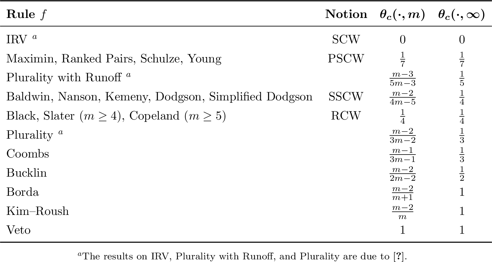
Table ¿tbl:tab:theo95results? reveals the existence of three clusters of voting rules sharing the same critical concentration parameter \(\theta_c(f,m)\), in addition to the IRV family, consisting of IRV and its variants, already identified by [5]. These clusters can be referred to as the Maximin family (Maximin, Ranked Pairs, Schulze, and Young), the Baldwin family (Baldwin, Nanson, Kemeny, Dodgson, and Simplified Dodgson), and the Black family (Black, Slater, and Copeland).

That some rules are grouped together is not entirely surprising, as several of them share closely related mechanisms—for instance Maximin, Ranked Pairs, and Schulze; Baldwin and Nanson; or Slater and Copeland. However, other aspects of the classification are less obvious a priori. In particular, it is not immediate that Young should belong to the Maximin family, or that Dodgson and Kemeny should be separated from it and instead cluster with Baldwin and Nanson. For Young, as discussed above, the connection with the Pair-Safe Condorcet Winner is non-trivial. For Kemeny and Dodgson, a closer inspection reveals that the number of swaps in the Dodgson rule, or the Kemeny score itself, can be related to scores in the weighted majority matrix, and therefore to the Borda scores used in Baldwin and Nanson. Finally, the position of the Black rule is particularly intriguing: it differs both from other Condorcet-consistent rules based on Borda elimination (Baldwin and Nanson) and from Borda itself.

Thus, the proposed classification is not immediately apparent from the axiomatic definitions of the rules. Whether it translates into similar behavior with respect to coalitional manipulation in real-world datasets is an empirical question, which we investigate next.

4 Numerical Results↩︎

The goal of this section is to test whether our simplified theoretical model retains explanatory power when confronted with real preference data. All code used in our experiments will be made available as a GitHub repository once this paper is published. We use two datasets, both introduced by [20].

• The Netflix dataset contains \(11{,}215\) profiles obtained by perturbing \(2{,}243\) base profiles, spanning \(m=3\) to \(m=11\) candidates and \(1{,}000\) to \(91{,}880\) voters. Preferences are cardinal and complete, and uniform random noise is used to break ties between equal ratings. Its size and coverage make it particularly suitable for detailed analyses that depend on \(m\).

• The FairVote dataset contains \(10{,}044\) profiles obtained by perturbing \(162\) base profiles, spanning \(m=3\) to \(m=11\) candidates and \(1{,}560\) to \(299{,}107\) voters. Preferences are ordinal and generally truncated, and uniform random noise is used to complete the truncated rankings. Although less rich, especially for larger values of \(m\), this dataset serves as a useful complement, as it describes real-world political elections.

Additional results on the more heterogeneous PrefLib dataset [27] are provided in the code repository, confirming the robustness of our findings.

Our numerical evaluations rely on SVVAMP, a Python package dedicated to studying the manipulability of voting rules [8], [9]. For each rule, the implemented manipulation algorithm classifies a profile as CM, non-CM, or undecided, meaning that the chosen algorithm cannot certify either outcome for that profile (algorithmic uncertainty). Compared to the version used by [20], the present work relies on a substantially improved version of the package. Namely, we implemented the notions of PSCW and SSCW, added five voting rules (Kemeny, Slater, Young, Dodgson, and Simplified Dodgson), and significantly improved the manipulation algorithms for five others (Ranked Pairs, Baldwin, Nanson, Copeland, and Kim–Roush).

We proceed in three steps. First, we examine the overall CM rates. Second, we compare how these rates vary with \(m\) against the theoretical predictions given by \(\theta_c(f,m)\). Finally, we focus on a fixed value of \(m\) to evaluate how well the theory predicts which rules are more resilient to coalitional manipulation.

4.1 Overall CM Rates↩︎

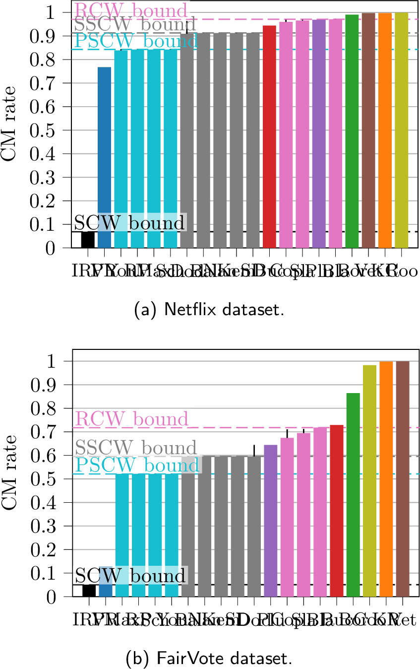
Figure 2 reports CM rates for the two datasets, restricted to profiles with at least five candidates, ensuring that our theoretical results apply to all voting rules. Additional figures for all values of \(m\) are provided in Appendix 9; conclusions are similar, except for Slater and Copeland as expected.

Compared to earlier work [20], our computations reduce uncertainty to very low levels for almost all rules, including NP-hard ones such as Kemeny, Slater, Dodgson, and Young [26], [28], [29]. Dodgson remains the least precise, with about 5% undecided cases in both datasets, followed by Copeland in the FairVote dataset (4%).

As already noted by [20], the absolute levels differ markedly across the two datasets, with profiles from the FairVote dataset being on average substantially less susceptible to coalitional manipulation. However, several common conclusions emerge.

First, the theoretical families identified in Table ¿tbl:tab:theo95results? also appear empirically: rules within a given family display very similar CM rates. Within the Maximin and Baldwin families, differences remain below 0.5% in both datasets. The only deviation arises from the upper bound of the uncertainty interval for Dodgson, while its lower bound remains consistent with the other rules in the Baldwin family. Within the Black family, the difference is at most 1% in the Netflix dataset, and ranges between 1% and 4% in the FairVote dataset, depending on uncertainty.

Second, just as the notion of SCW explains most non-CM cases for IRV [5], the notions of PSCW, SSCW, and RCW provide tight explanations for specific families. For example, the CM rates of the Maximin family closely align with the absence of a PSCW. In the particular case of Dodgson, we recall that despite sharing the same critical concentration parameter as the rest of the Baldwin family, it is theoretically unaffected by the SSCW bound (Section 3.2). Unfortunately, algorithmic uncertainty prevents us from determining whether counterexamples in which Dodgson is susceptible to coalitional manipulation despite the existence of an SSCW are frequent.

Third, an unexpected pattern emerges: in both datasets, Kim–Roush and Veto exhibit very similar, near-maximal CM rates. We return to this observation below.

4.2 Variation with the Number of Candidates↩︎

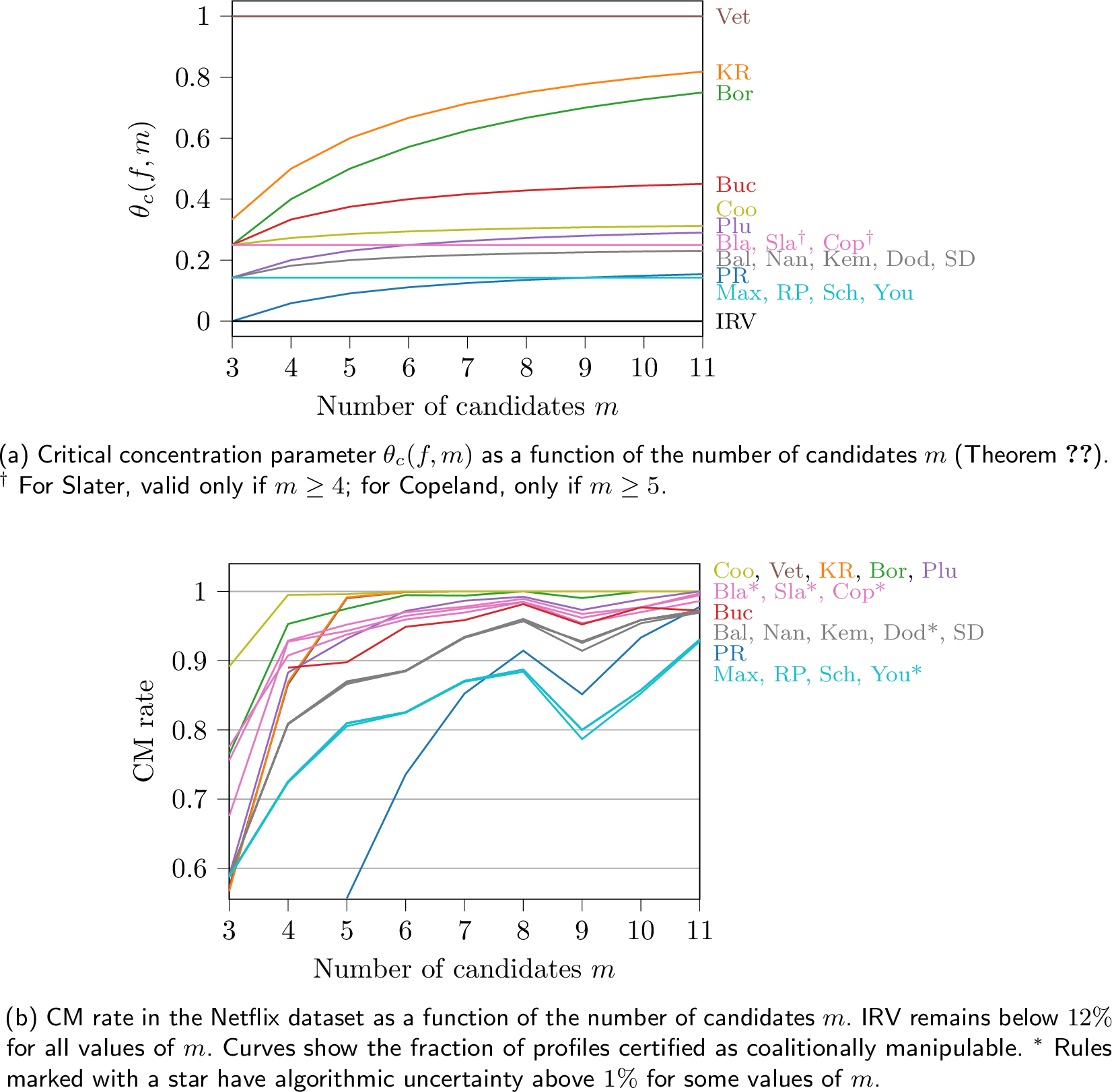
We now examine how coalitional manipulability varies with the number of candidates \(m\), combining theoretical predictions (Fig. [plot95theoretical95results]) with empirical results (Fig. [netflix95selected95rules95nb95candidates95rate95line95plot]). We focus on the Netflix dataset, which contains a relatively large number of base profiles even for larger \(m\) (e.g., 72 base profiles for \(m=11\)). We also include profiles with three or four candidates, noting that tie-breaking then significantly affects Slater and/or Copeland. IRV is not visible in Fig. [netflix95selected95rules95nb95candidates95rate95line95plot], as its CM rates remain below 12%.

Both Figures exhibit common patterns. Rules within each of the Maximin, Baldwin, and Black families display very similar CM rates across all values of \(m\). Plurality with Runoff coincides with IRV at \(m=3\) (by definition), and then crosses the Maximin family as predicted, with a slightly shifted crossing point (\(m=9\) in theory and \(m \in [7,8]\) in practice). The Maximin family, the Baldwin family, and Plurality coincide at \(m=3\) but stratify thereafter in that order, with Plurality eventually performing worse than the Black family. The Black family consistently performs worse than the Baldwin family, while Borda starts at the same level as the Black family but degrades further as \(m\) increases. Overall, the theory provides a faithful qualitative description of the behavior of IRV, the Maximin family, Plurality with Runoff, the Baldwin family, the Black family, Plurality, and Borda.

Some discrepancies nevertheless emerge. In Figure [netflix95selected95rules95nb95candidates95rate95line95plot], Kim–Roush and Veto are almost indistinguishable empirically, a behavior reminiscent of their identical asymptotic CM rate under Impartial Culture [14]. For larger values of \(m\), both rules behave as expected and are more vulnerable than Borda. For smaller \(m\), however, they appear less manipulable than predicted when compared to other rules. Coombs is consistently more manipulable than predicted, whereas Bucklin performs worse than expected at \(m=3\) but better for larger \(m\).

For veto-based rules, these deviations likely stem from peculiarities of the Perturbed Culture at the bottom of the rankings: candidate 1 is not favored, receiving as many bottom votes as candidates \(\{2,\ldots,m-1\}\), while only candidate \(m\) is disadvantaged. For Bucklin, a similar effect occurs beyond the first rank: at rank 2 the model favors candidate 2, at rank 3 candidate 3, and so on. Alternative models such as Mallows may be better suited to study these rules, though at higher technical cost.

4.3 Comparison of Voting Rules for Fixed \(m\)↩︎

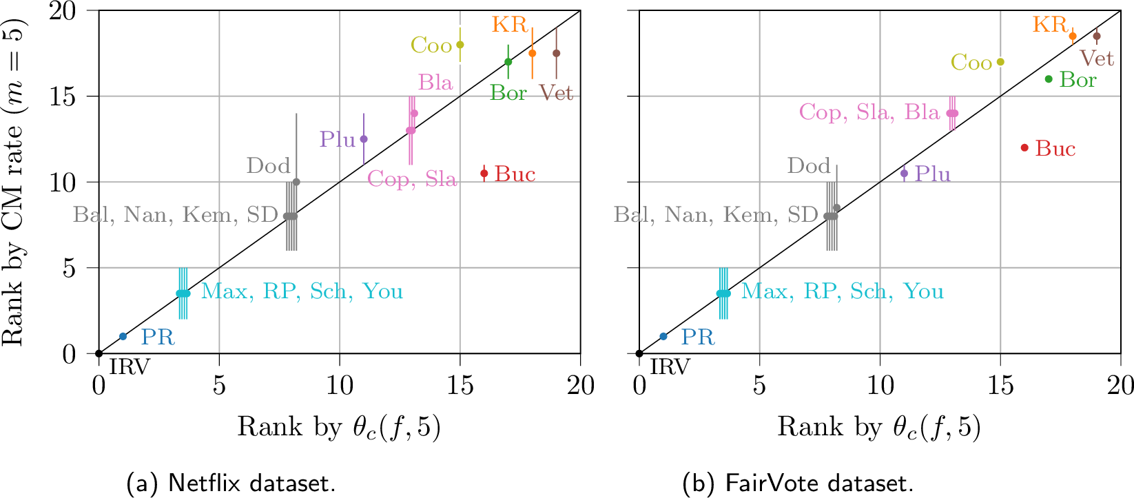
For a fixed number of candidates \(m\), the critical concentration parameter \(\theta_c(f,m)\) induces a theoretical ordering of voting rules. A natural question is whether this theoretical ordering has predictive power for the ordering induced by their empirical CM rates. Figure [fig:netflix95selected95rules95scatter95rank95theta95c95rank95cm95rate] confronts these two rankings for the Netflix dataset, while Figure [fig:fairvote95selected95rules95scatter95rank95theta95c95rank95cm95rate] does so for the FairVote dataset. We fix \(m=5\), the smallest value for which all our theoretical results apply, including Slater and Copeland. Analogous plots for larger values of \(m\) are provided in the code repository.

By convention, the minimal rank is set to 0. For the theoretical ranking based on \(\theta_c(f,5)\), ties correspond to exact equalities and are assigned the average rank (e.g., the four rules tied for ranks 2 to 5 each receive rank 3.5). For empirical CM rates, uncertainty arises from two sources: algorithmic limitations and differences below 1%, which are treated as non-significant; both effects are reflected in the error bars. Finally, for readability, rules sharing the same value of \(\theta_c(f,5)\) are displayed with a slight horizontal offset.

In both figures, the agreement is strong: the ranking predicted by the critical concentration parameter closely matches the empirical ranking. The main exceptions are Bucklin and Coombs, in line with the discrepancies already identified in the previous subsection. For Veto and Kim–Roush, as already observed for larger values of \(m\), the theory correctly predicts their position in the ranking at \(m=5\), but not their near-identical empirical CM rates. Finally, the ordinal conclusions are remarkably similar across the two datasets, despite large differences in absolute CM rates (Section 4.1).

Overall, this experiment shows that the model has genuine predictive power over the relative vulnerability of voting rules to coalitional manipulation, despite the absence of any parameter fitting: the only input provided to the model is the number of candidates \(m\). The key intuition is that elections typically feature a candidate who is globally stronger than the others in the preferences of the voters, a phenomenon captured in the model by the concentration parameter. When this advantage is sufficiently large, a voting rule becomes immune to coalitional manipulation; what counts as “sufficiently large” depends on the rule and is captured in the theoretical model by its critical concentration parameter. This explains why, for a fixed \(m\), we recover essentially the same ordering of voting rules across datasets, even when their absolute CM rates differ substantially. It is very plausible that other probabilistic models built on the same basic ingredients, such as the Mallows model, would lead to similar conclusions. The strength of the Perturbed Culture lies in its ability to deliver these insights while remaining particularly tractable mathematically.

5 Future work↩︎

A first direction for future work is to test the robustness of our results under alternative preference models, such as Mallows, Bradley–Terry, Plackett–Luce, spatial models, or mixtures thereof, and to examine whether some of these models better explain the behavior of Bucklin, Veto, Coombs, and Kim–Roush. Another natural step is to design probabilistic models that are also suitable for non-ordinal rules, such as Range Voting. It would also be valuable to study the critical regime \(\theta=\theta_c(f,m)\) in more detail, in particular to determine whether the bounds derived from our strengthened Condorcet notions remain tight at the phase transition. Beyond coalitional manipulation, phase transitions in parametric cultures could further shed light on other voting paradoxes, such as violations of monotonicity, participation, or independence of irrelevant alternatives.

.tocapp

Technical Appendix↩︎

In this technical appendix, we elaborate on some points of the paper that are omitted from the main text for the sake of conciseness and clarity. We also include two additional Condorcet-consistent voting rules, defined as follows.

Split Cycle (SC). With the same notation as for the Schulze rule (Section 2.2.5), elect a candidate \(c\) such that \(\textrm{Strength}(c,d,P) \geq W(d,c,P)\) for all \(d\) [30].

Viennot (Vie). At each round, select the two candidates with the lowest plurality scores and eliminate the one losing their pairwise contest [2], [20].

We will see that these two rules naturally belong to the Maximin family, both theoretically and experimentally. Split Cycle relies on a mechanism very close to that of the Schulze rule; we chose to exclude it from the main paper to avoid redundancy, but include it here for the sake of completeness. The Viennot rule is less studied, but provides a particularly interesting case in our framework: although the existence of a PSCW is neither necessary nor sufficient for immunity to coalitional manipulation, the rule shares the same critical concentration parameter as the Maximin family. The fact that it exhibits very similar empirical CM rates (Section 9) shows that this empirical clustering of voting rules cannot be attributed solely to the PSCW notion, but also reflects the predictive power of the critical concentration parameter itself.

Before proceeding, we briefly recall the main notation used throughout the appendices. For any (discrete or continuous) profile \(P\), \(w(P)\) denotes its total weight. We also write \(w(P^{\psi})\) for the weight of the subpopulation of voters whose rankings satisfy a condition \(\psi\); typical examples include \(w(P^{c \succ d})\) and \(w(P^{c \succ d \text{ and } c \succ e})\). The notation \(s_f\) denotes a notion of score for rule \(f\), whereas \(p_f\) denotes a notion of penalty. For any pair of candidates \((c,d)\), \(W(c,d,P) = w(P^{c \succ d})\) denotes the total weight of voters preferring \(c\) to \(d\); the matrix \(W(P)\) with entries \(W(c,d,P)\) is the weighted majority matrix of \(P\).

For reference, we recall where the strengthened notions of Condorcet winner used in the paper are defined: the SCW in Equation 1 ; the PSCW in Equation ?? ; the SSCW in Equations ?? , ?? , ?? , and ?? ; and the RCW in Equation 2 .

Finally, we introduce the notation \(b(\epsilon)\) (read “bounded by epsilon”) to denote a real number whose absolute value is at most \(\epsilon\).

Appendix 6 provides a detailed analysis of the examples used throughout the paper. Appendix 7 presents the theoretical preliminaries, while Appendix 8 contains the proofs of the paper’s main results. Finally, Appendix 9 reports additional figures showing global CM rates, including the cases \(m \in \{3,4\}\) and the two additional voting rules.

6 Examples↩︎

This section provides a detailed verification of all examples discussed in the main body of the paper. Each table is recalled with an extended caption summarizing its relevant properties, which are then checked explicitly. This analysis also serves to illustrate the strengthened Condorcet notions discussed in the paper.

6.1 Analysis of Table ¿tbl:tab:ex_scw_no_pscw_rules_not_CM?↩︎

\(\begin{array}{ccc} \hline 5 & 4 & 2 \\ \hline B & A & C \\ A & C & A \\ C & B & B \\ \hline \end{array}\)

The profile in Table ¿tbl:tab:ex_scw_no_pscw_rules_not_CM_remind? consists of \(n(P) = w(P) = 11\) voters.

Candidate \(A\) is the SCW, as defined in Equation 1 , since \[\begin{align} s_\textrm{Plu}(A, P_{\{A,B,C\}}) &= 4 > 11/3,\\ s_\textrm{Plu}(A, P_{\{A,B\}}) &= 6 > 11/2,\\ s_\textrm{Plu}(A, P_{\{A,C\}}) &= 9 > 11/2. \end{align}\]

Candidate \(A\) is not a PSCW, as defined in Equation ?? , since \[w(P^{A \succ B \text{ and } A \succ C}) = 4 \quad\text{and}\quad w(P^{B \succ A}) = 5,\] hence \(w(P^{A \succ B \text{ and } A \succ C}) \le w(P^{B \succ A})\). Intuitively, if all voters preferring \(B\) to \(A\) demote \(A\) below \(C\) in their ranking, only the voters in \(P^{A \succ B \text{ and } A \succ C}\) still support \(A\) in the pairwise comparison against \(C\), which then becomes a defeat more severe than that of \(B\) against \(A\).

If a candidate \(A'\) is added just below \(A\) in every ranking, it is straightforward to verify that \(A\) remains an SCW but is still not a PSCW.

Since all the rules mentioned here are Condorcet-consistent, \(A\) is elected. We now show that the profile is immune to coalitional manipulation for all these rules.

Consider a manipulation attempt in favor of \(B\). Only the voters in the first column can participate in such a manipulation. However, they cannot prevent \(B\) from being a Condorcet loser, i.e., a candidate who suffers pairwise defeats against all others. Since \(m=3\) and \(n\) is odd, this implies that another candidate must be the Condorcet winner and is therefore elected. For Copeland and Slater, the example includes the additional candidate \(A'\); it then suffices to note that these rules can never elect a Condorcet loser, which prevents \(B\) from winning.

We now consider a manipulation attempt in favor of \(C\), which may involve the voters in the third column. Table ¿tbl:tab:ex95scw95no95pscw95rules95not95CM95manipulated95wmm? reports bounds on the entries of the weighted majority matrix of a potential target profile \(Q\). When displaying a majority matrix, we always omit the diagonal coefficients for legibility.

\(\begin{array}{c|c|c|c|} & A & B & C \\ \hline A & & [4, 6] & [9, 11] \\ \hline B & [5,7] & & [5,7] \\ \hline C & [0,2] & [4,6] & \\ \hline \end{array}\)

We now show that, for each rule listed in the caption of Table ¿tbl:tab:ex_scw_no_pscw_rules_not_CM_remind?, this manipulation attempt fails, as candidate \(C\) cannot be elected in \(Q\).

6.1.0.1 Max, RP, Sch, SC

\(\min\{W(A,B,Q),\, W(A,C,Q)\} > W(C,A,Q)\). Since all four rules are Maximin-like, \(C\) cannot win in \(Q\).

6.1.0.2 Vie

The manipulators cannot prevent \(C\) from being selected for the first-round duel, so \(C\) must face \(A\) and then \(B\), or vice versa, in pairwise comparisons. However, \(C\) necessarily loses its pairwise comparison against \(A\), which prevents it from being elected.

6.1.0.3 You

We bound the penalties after manipulation. For \(A\), we can keep at least the voters of the second column and three others, that is, 7 voters in total; hence \(p_\textrm{You}(A, Q) \le 11 - 7 = 4\). For \(C\), to win against \(A\), at most the two voters of the last column and one additional voter can stay, yielding \(p_\textrm{You}(C, Q) \ge 11 - 3 = 8\). Therefore, \(p_\textrm{You}(C, Q) > p_\textrm{You}(A, Q)\).

6.1.0.4 Bal, Nan

We have \(s_\textrm{Bor}(A, Q) \ge 13\), \(s_\textrm{Bor}(B, Q) \ge 10\), and finally \(s_\textrm{Bor}(C, Q) \le 8\). Hence, \(C\) is eliminated in the first round.

6.1.0.5 Dod, SD

We bound the penalties after manipulation. Candidate \(C\) needs at least four swaps to win against \(A\), hence \(p_f(C, Q) \ge 4\). Candidate \(A\) already beats \(C\), and two swaps among the voters in the left column are sufficient for \(A\) to win against \(B\), so \(p_f(A, Q) \le 2\). Therefore, \(p_f(C, Q) > p_f(A, Q)\).

6.1.0.6 Kem

If \(C\) were the winner, moving it to the bottom of the ranking would change the penalty by an amount \(W(C,A,Q) + W(C,B,Q) - W(A,C,Q) - W(B,C,Q) \le 2 + 6 - 9 - 5 = -6 < 0.\) There would thus exist a strictly better ranking, contradicting the optimality of the winning ranking.

6.1.0.7 Cop, Sla

As with all Condorcet-consistent voting rules, the existence of an RCW implies that Copeland and Slater are immune to coalitional manipulation. This example will show that the converse is false: these rules are immune to CM, even though the winner \(A\) is not an RCW, and in fact not even a PSCW.

Recall that we consider the version of the example including the additional candidate \(A'\). Candidate \(C\) has at most one victory (against \(B\)), and thus cannot win under Copeland, since another candidate has at least two victories. For Slater with \(m=4\), a candidate with at most one victory can likewise never win, as we now show. If a candidate has three victories, it is the Condorcet winner and therefore wins. Otherwise, the vector of numbers of victories (Copeland scores) is either \((2,2,2,0)\) or \((2,2,1,1)\). The first case is straightforward, as there is then a Condorcet loser. Let us therefore examine the second one. Label the two candidates with two victories \(a\) and \(b\) such that \(a\) beats \(b\). Consequently, the two victories of \(b\) are against the other two candidates, denoted \(c\) and \(d\). Without loss of generality, assume that \(c\) beats \(d\); then the only victory of \(d\) must be against \(a\). It is easy to verify that the order \((a \succ b \succ c \succ d)\) is the unique ranking with minimal Slater penalty, equal to 1. Hence, none of the candidates with a single victory can be the Slater winner. Finally, it remains to check that no manipulation in favor of \(A'\) is possible, which is trivial since no voter prefers \(A'\) to \(A\).

6.2 Analysis of Table ¿tbl:tab:ex_you_is_not_maximin_like?↩︎

\(\begin{array}{c c c} \hline 30 & 72 & 72 \\ \hline A & C_\bullet & B \\ B & C_\bullet & C_\bullet \\ C_\bullet & A & C_\bullet \\ C_\bullet & B & A \\ C_\bullet & C_\bullet & C_\bullet \\ \hline \end{array}\)

\(\begin{array}{c|c|c|c|c|c|} & A & B & C_1 & C_2 & C_3 \\ \hline A & & 102 & 78 & 78 & 78 \\ \hline B & 72 & & 126 & 126 & 126 \\ \hline C_1 & 96 & 48 & & 87 & 87 \\ \hline C_2 & 96 & 48 & 87 & & 87 \\ \hline C_3 & 96 & 48 & 87 & 87 & \\ \hline \end{array}\)

We now turn to the example of Table ¿tbl:tab:ex_you_is_not_maximin_like_remind?, whose weighted majority matrix is given in Table ¿tbl:tab:ex95you95is95not95maximin95like95wmm?. We have \(\min_e W(A, e, P) = 78\) and \(W(B, A, P) = 72\), hence \(\min_e W(A, e, P) > W(B, A, P)\).

6.2.0.1 You

For candidate \(A\), it is most effective to remove voters from the second column. To make \(A\) win against each candidate \(C_i\), more than \(96 - 78 = 18\) points must be removed in each of the three corresponding pairwise comparisons, that is, more than \(54\) points in total. However, each ballot removed deprives the \(C_i\)’s of two points while also costing \(A\) one point against a \(C_i\). Hence, more than 54 ballots must be removed, so \(p_\textrm{You}(A, P) > 54\). For candidate \(B\), it suffices to remove the voters of the first column and one additional arbitrary voter, giving \(p_\textrm{You}(B, P) = 31\). For each candidate \(C_i\), it is necessary to win against \(B\), so \(p_\textrm{You}(C_i, P) > 126 - 48 = 78\). Therefore, \(B\) is elected.

6.2.0.2 Vie

The first-round plurality scores are \(\{A: 30, B: 72, C_1: 24, C_2: 24, C_3: 24\}\). One candidate \(C_k\) loses to some \(C_j\). At the second round, the plurality scores are \(\{A: 30, B: 72, C_i: 36, C_j: 36\}\). Candidates \(A\) and, say, \(C_j\) are selected, and \(A\) is eliminated. Since \(B\) is the Condorcet winner in the remaining profile, it is elected.

6.3 Analysis of Table ¿tbl:tab:ex_pscw_no_sscw?↩︎

\(\begin{array}{c c c c} \hline 2 & 6 & 5 & 6 \\ \hline A & B & C & D \\ B & A & A & A \\ C & C & B & B \\ D & D & D & C \\ \hline \end{array}\)

In the example of Table ¿tbl:tab:ex_pscw_no_sscw_remind?, we have \[\begin{align} w(P^{A \succ B \text{ and } A \succ C}) &= 8, \qquad\qquad w(P^{B \succ A}) = 6,\\ w(P^{A \succ B \text{ and } A \succ D}) &= 7, \qquad\qquad w(P^{C \succ A}) = 5,\\ w(P^{A \succ C \text{ and } A \succ D}) &= 8, \qquad\qquad w(P^{D \succ A}) = 6,\\ \end{align}\] hence \(w(P^{A \succ B \text{ and } A \succ C}) > w(P^{B \succ A})\), and similarly for any pair of candidates distinct from \(A\). Therefore, \(A\) is the PSCW, as defined in Equation ?? .

On the other hand, evaluating Equation ?? for the candidate of interest \(c = A\) and the opponent \(d = B\), we obtain \[\begin{align} & w(P^{A \succ B}) - \tfrac{19}{2} + w(P^{A \succ B \text{ and } A \succ C}) - \tfrac{19}{2} + w(P^{A \succ B \text{ and } A \succ D}) - \tfrac{19}{2} \\ &= 13 - \tfrac{19}{2} + 8 - \tfrac{19}{2} + 7 - \tfrac{19}{2} \\ &= - \tfrac{1}{2}, \end{align}\] hence \(A\) is not an SSCW. Intuitively, in a manipulation attempt in favor of \(B\), the manipulators can make the cumulative defeats of \(A\) against \(C\) and \(D\) outweigh the defeat that \(B\) suffers against \(A\).

In Viennot, candidate \(A\) wins since it is the Condorcet winner. If the voters in the second column move \(A\) to the bottom of their ranking, the first round still selects \(A\) and \(C\), but \(A\) is then eliminated. Candidate \(B\) becomes the Condorcet winner in the remaining profile and is therefore elected.

6.4 Analysis of Table ¿tbl:tab:ex_sscw_no_rcw_dod_cm?↩︎

\(\begin{array}{c c c c} \hline 40 & 36 & 12 & 12 \\ \hline A & B & C & C \\ B & A & D & D' \\ C & C & A & A \\ D & D & B & B \\ D' & D' & D' & D \\ \hline \end{array}\)

We now examine the example of Table ¿tbl:tab:ex_sscw_no_rcw_dod_cm_remind?. Evaluating Equation ?? for the candidate of interest \(c = A\) and the opponent \(d = B\), we obtain \[\begin{align} & w(P^{A \succ B}) - 50 + \sum_e \min(0,\, w(P^{A \succ B \text{ and } A \succ e}) - 50) \\ &= (64 - 50) + \min(0, 40 - 50) + \min(0, 52 - 50) + \min(0, 52 - 50) \\ &= 4 > 0, \end{align}\] which satisfies the SSCW condition. Similarly, the same condition can be verified for opponents \(C\) and \(D\). Therefore, \(A\) is an SSCW.

However, we have \[w(P^{A \succ B \text{ and } A \succ C}) = 40 \le 50,\] hence \(A\) is not an RCW.

Let us show that Dodgson is susceptible to coalitional manipulation in favor of \(B\). Consider a target profile \(Q\) where all voters in the second column simply move \(A\) to the bottom of their ranking. Candidate \(B\) already beats \(C\), \(D\), and \(D'\), and overturning the defeat of \(B\) against \(A\) can be achieved with 15 swaps in the first column. Hence \(p_\textrm{Dod}(B, Q) = 15\). Candidate \(A\) has only 40 points against \(C\), thus requiring at least \(51 - 40 = 11\) useful swaps. The most effective operation is to perform them in one of the two last columns, but each useful swap must first be preceded by a useless swap between \(A\) and \(D\) or \(D'\), so \(p_\textrm{Dod}(A, Q) \ge 22\). Candidate \(C\) has only 24 points against \(B\), hence \(p_\textrm{Dod}(C, Q) \ge 27\). Candidate \(D\) has only 12 points against \(B\), hence \(p_\textrm{Dod}(D, Q) \ge 39\), and similarly for \(D'\). Therefore, \(B\) is elected.

6.5 Analysis of Table ¿tbl:tab:ex_rcw_no_scw?↩︎

\(\begin{array}{c c c c c} \hline 1 & 2 & 2 & 2 & 2 \\ \hline A & B_1 & B_2 & B_3 & B_4 \\ & A & A & A & A \\ \vdots & \vdots & \vdots & \vdots & \vdots \\ \hline \end{array}\)

In the example of Table ¿tbl:tab:ex_rcw_no_scw_remind?, for any \(i\neq j\) we have \(w(P^{A \succ B_i \text{ and } A \succ B_j}) = 5 > 9/2\); hence candidate \(A\) is the RCW, as defined in Equation 2 . On the other hand, \(s_\textrm{Plu}(A, P) = 1 \le 9/5\), so candidate \(A\) violates the SCW condition defined in Equation 1 for the set \(K = \mathcal{C}(P)\).

7 Theoretical Preliminaries↩︎

Section 7.1 states a collection of lemmas that are used repeatedly to establish the asymptotic behavior of the different voting rules. Section 7.2 analyzes the expected profile. Section 7.3 then restricts this profile to voters who prefer candidate 1 to candidate 2 and therefore remain sincere under a manipulation in favor of 2 against 1. Finally, Section 7.4 studies a simple manipulation strategy by voters preferring 2 to 1, which suffices to establish the sub-critical regime for a significant number of voting rules. We assume throughout that \(m \ge 3\), as the case \(m=2\) is trivial for all rules in our analysis.

7.1 Manipulation Lemmas↩︎

The proofs of [5] rely on three lemmas. We restate them here with minor rephrasing, in order to facilitate their later generalization. Recall that \(\hat{P}\) denotes the expected normalized profile (or simply the expected profile), in which each ranking has weight \(\tfrac{1-\theta}{m!}\), except for the reference ranking \((1 \succ \cdots \succ m)\), which has weight \(\theta + \tfrac{1-\theta}{m!}\).

Before stating the second lemma, we recall the notion of unison manipulation [5], [20], [31]. A voting rule \(f\) is said to be unison-manipulable (UM) in a profile \(P\) (or equivalently, \(P\) is UM under \(f\)) if a manipulation can succeed even when all interested voters cast the same ballot (see Section 7.4 for an example).

Before introducing the third lemma, we recall the notion of \(\delta\)-stable coalitional manipulability [5], for any \(\delta > 0\). A rule \(f\) is said to be \(\delta\)-stable-CM in a continuous profile \(P\) (or equivalently, \(P\) is \(\delta\)-stable-CM in \(f\)) if there exists a continuous profile \(Q\) such that:

• \(f\) is CM from \(P\) to \(Q\), and

• for any profile \(Q'\) with \(d_\infty(Q, Q') < \delta\), we have \(f(Q') = f(Q)\).

Here, \(d_\infty(Q, Q')\) denotes the \(\ell^\infty\) distance between profiles, viewed as vectors of weights. Intuitively, \(f\) is CM from \(P\) to \(Q\) with an outcome that is stable close enough to \(Q\).

The general proof strategy is as follows, for some value \(\theta^*\) conjectured to be the critical concentration parameter:

• show that candidate 1 wins in a neighborhood of \(\hat{P}\);

• show that for \(\theta > \theta^*\) the rule is non-CM in a neighborhood of \(\hat{P}\), allowing us to apply Lemma 1;

• show that for \(\theta < \theta^*\) the rule is UM or \(\delta\)-stable-CM in a neighborhood of \(\hat{P}\), allowing us to apply Lemma 2 or 3.

We may then conclude that the rule admits the critical parameter \(\theta_c(f, m) = \theta^*\). Variants of this strategy are sometimes required, for instance when candidate 1 does not win in a neighborhood of \(\hat{P}\) (see Section 8.5).

If a rule is defined only on discrete profiles, as is the case for Young, Dodgson, and Simplified Dodgson, we proceed similarly. However, we cannot work directly with \(\hat{P}\) or with continuous profiles in its neighborhood. Instead, we consider discrete profiles \(P\) whose normalized version \(\bar{P}\) lies close to \(\hat{P}\). We then use the following generalized lemmas, which are proved in exactly the same way using the weak law of large numbers. Differences with the original statements are highlighted in bold.

In all cases, the convergence is exponentially fast, by the same concentration argument as in [5], relying on Hoeffding’s inequality.

7.2 Expected Profile↩︎

In this section, we analyze the expected profile \(\hat{P}\), which will be used in many subsequent proofs. Its weighted majority matrix \(W(\hat{P})\) is shown in Table ¿tbl:tab:wmm95original?. Candidate 1 is the Condorcet winner; since this conclusion relies on strict inequalities, it remains valid in a neighborhood of \(\hat{P}\), and therefore also holds for the random profile \(P\) with high probability by the weak law of large numbers.

\(\begin{array}{c|c|c|c|c|} & 1 & 2 & j & k \\ \hline 1 & & \frac{1}{2}(1-\theta) + \theta & \frac{1}{2}(1-\theta) + \theta & \frac{1}{2}(1-\theta) + \theta \\ \hline 2 & \frac{1}{2}(1-\theta) & & \frac{1}{2}(1-\theta) + \theta & \frac{1}{2}(1-\theta) + \theta \\ \hline j & \frac{1}{2}(1-\theta) & \frac{1}{2}(1-\theta) & & \frac{1}{2}(1-\theta) + \theta \\ \hline k & \frac{1}{2}(1-\theta) & \frac{1}{2}(1-\theta) & \frac{1}{2}(1-\theta) & \\ \hline \end{array}\)

For two distinct opponents of candidate 1, denoted \(c\) and \(d\), note that the \((1-\theta)\) purely random voters (the “IC part”) treat these candidates symmetrically, whereas the remaining \(\theta\) voters (the “Dirac part”) all rank candidate 1 first. Hence, \[w(\hat{P}^{1 \succ c \text{ and } 1 \succ d}) = \tfrac{1}{3}(1-\theta) + \theta,\] a useful quantity that appears in several strengthened notions of Condorcet winner.

7.3 Expected Profile Restricted to \(1 \succ 2\)↩︎

For most of the rules considered in this paper, candidate 1 is the winner in the expected profile \(\hat{P}\). Candidate 2 then naturally emerges as the main challenger, and we will frequently examine manipulation attempts in favor of 2. As a preliminary step, we study the contribution of the sincere voters, that is, those who rank candidate 1 above 2 in \(\hat{P}\). The corresponding weighted majority matrix \(W(\hat{P}^{1 \succ 2})\) is given in Table ¿tbl:tab:wmm95sincere95voters? for later reference.

\(\begin{array}{c|c|c|c|c|} & 1 & 2 & j & k \\ \hline 1 & & \frac{1}{2}(1-\theta) + \theta & \frac{1}{3}(1-\theta) + \theta & \frac{1}{3}(1-\theta) + \theta \\ \hline 2 & 0 & & \frac{1}{6}(1-\theta) + \theta & \frac{1}{6}(1-\theta) + \theta \\ \hline j & \frac{1}{6}(1-\theta) & \frac{1}{3}(1-\theta) & & \frac{1}{4}(1-\theta) + \theta \\ \hline k & \frac{1}{6}(1-\theta) & \frac{1}{3}(1-\theta) & \frac{1}{4}(1-\theta) & \\ \hline \end{array}\)

7.4 A Simple Manipulation Strategy↩︎

When candidate 1 is the original winner, a simple manipulation strategy in favor of candidate 2 consists in casting the ballot \((2 \succ \cdots \succ m \succ 1)\). Let \(Q\) denote the profile obtained from \(\hat{P}\) when all voters who sincerely prefer candidate 2 to candidate 1 cast this ballot. The corresponding weighted majority matrix \(W(Q)\) is shown in Table ¿tbl:tab:wmm95um952? and will be used in several proofs.

\(\begin{array}{c|c|c|c|c|} & 1 & 2 & j & k \\ \hline 1 & & \frac{1}{2} (1-\theta) + \theta & \frac{1}{3} (1-\theta) + \theta & \frac{1}{3} (1-\theta) + \theta \\ \hline 2 & \frac{1}{2} (1-\theta) & & \frac{2}{3} (1-\theta) + \theta & \frac{2}{3} (1-\theta) + \theta \\ \hline j & \frac{2}{3} (1-\theta) & \frac{1}{3} (1-\theta) & & \frac{3}{4} (1-\theta) + \theta \\ \hline k & \frac{2}{3} (1-\theta) & \frac{1}{3} (1-\theta) & \frac{1}{4} (1-\theta) & \\ \hline \end{array}\)

8 Proofs of Theoretical Results↩︎

This appendix provides proofs of all theoretical results stated in the paper, and also establishes the corresponding results for Split Cycle and the Viennot rule. As in the previous section, we always assume \(m \geq 3\).

8.1 Maximin family: Maximin, Ranked Pairs, Schulze, Split Cycle, Young, Viennot↩︎

We analyze here the Maximin family. We first study the properties of Split Cycle and the Young rule in Sections 8.1.1 and 8.1.2. In Section 8.1.3, we then determine the common critical concentration parameter of the family, except for the Viennot rule, which is not structurally related to the Pair-Safe Condorcet Winner and is therefore treated separately in Section 8.1.4.

8.1.1 Split Cycle is Maximin-like↩︎

As for Maximin, Ranked Pairs, and Schulze (Proposition [thm:maximin95like95which95rules]), it is straightforward to verify that Split Cycle is Maximin-like. Consequently, by Theorem [thm:maximin95like95rules95property], if a PSCW exists, then Split Cycle is immune to coalitional manipulation. Here again, the converse does not hold, as illustrated by Table ¿tbl:tab:ex_scw_no_pscw_rules_not_CM?, analyzed in Section 6.1: the profile admits no PSCW, yet Split Cycle remains immune to coalitional manipulation.

8.1.2 The Young rule and the PSCW↩︎

In the main body, the Young rule was defined in the most common way, through the notion of penalty. For the purpose of the result below, it is convenient to express it in terms of a Young score: \[s_\textrm{You}(c, P) = \begin{cases} n(P) - p_\textrm{You}(c, P), & \text{if c is not a CW,}\\[4pt] 2 \min_{d \neq c}\big(w(P^{c \succ d})\big) - 1, & \text{if c is a CW.} \end{cases}\]

The first expression conveys the main intuition: rather than counting the minimal number of voters that must be removed so that \(c\) becomes a Condorcet winner, it represents the maximal number of voters that can be kept.

The second expression can be interpreted through the following thought experiment. In addition to the voters in \(P\), consider an infinite pool of virtual voters who all rank \(c\) last. We then ask for the maximal number of voters that can be selected so that \(c\) is a Condorcet winner, either from \(P\) or from this additional pool. This thought experiment also applies to the first case.

Finally, recall that if \(c\) can never be a Condorcet winner, we defined by convention \(p_\textrm{You}(c, P) = n(P) + 1\). This falls under the first case above and yields \(s_\textrm{You}(c, P) = -1\), which can be interpreted as follows: not only can no voter be selected from \(P\) or from the additional pool, but one would even need to add a hypothetical anti-voter from the virtual pool, that is, a voter who ranks \(c\) first.

This definition is convenient because it provides simple bounds. For any opponent \(d\), candidate \(c\) must defeat \(d\) in pairwise comparison; hence \[\label{eq:young95score95upper95bound} s_\textrm{You}(c, P) \le 2\, w(P^{c \succ d}) - 1.\tag{3}\] On the other hand—and this is where the second case of our definition proves useful—considering the rankings where \(c\) is placed first yields a lower bound on the Young score: \[\label{eq:young95score95lower95bound} s_\textrm{You}(c, P) \ge 2\, w(P^{r(c) = 1}) - 1.\tag{4}\] We will use variants of this bound in the proof below.

We already proved that the Young rule is not Maximin-like (Table ¿tbl:tab:ex_you_is_not_maximin_like?, analyzed in Section 6.2). It remains to prove the second part of the proposition.

8.1.3 Critical concentration parameters↩︎

We now analyze the asymptotic behavior of the PSCW notion and of the Maximin family under the Perturbed Culture model, excluding the Viennot rule, whose analysis requires a substantially different proof and is therefore deferred to Section 8.1.4.

In the subsequent proofs, unless stated otherwise, we will restrict attention to the normalized profile and leave the end of the argument implicit—namely, that the reasoning relies on strict inequalities involving continuous quantities and therefore holds in a neighborhood.

An immediate consequence of Theorem [thm:theta95critical95pscw] is Corollary [thm:theta95u95if95protected95by95pscw].

We can finally prove the existence of a phase transition and determine the corresponding critical concentration parameter for the rules of the Maximin family, except the Viennot rule.

8.1.4 The Viennot rule↩︎

Like the Young rule, but unlike the other rules in the Maximin family, the Viennot rule is not Maximin-like (Table ¿tbl:tab:ex_you_is_not_maximin_like?, analyzed in Section 6.2). Moreover, unlike the Young rule, the existence of a PSCW does not even guarantee immunity to coalitional manipulation (Table ¿tbl:tab:ex_pscw_no_sscw?, analyzed in Section 6.3). Conversely, the Viennot rule may still be immune to coalitional manipulation without a PSCW (Table ¿tbl:tab:ex_scw_no_pscw_rules_not_CM?, analyzed in Section 6.1). Nevertheless, its critical concentration parameter is equal to \(\tfrac{1}{7}\), but for a different reason. Intuitively, when manipulating in favor of candidate 2, this value corresponds to the threshold below which manipulators can force an elimination duel between candidates 1 and 3. It then becomes relatively easy to eliminate candidate 1 in that pairwise comparison. Once candidate 1 is eliminated, the path is clear for candidate 2.

8.2 Baldwin family: Baldwin, Nanson, Kemeny, Dodgson, Simplified Dodgson↩︎

We now turn to the Baldwin family. We recall that the rules in this family are immune to coalitional manipulation whenever a Set-Safe Condorcet Winner exists (Proposition [thm:baldwin95nanson95kemeny95sscw]), except Dodgson.

An immediate consequence of Theorem [thm:theta95critical95sscw] is Corollary [thm:theta95u95if95protected95by95sscw].

We can now establish the phase transition phenomenon for the rules of the Baldwin family. Although Dodgson is not rendered immune to coalitional manipulation by the existence of an SSCW, its similarity with Simplified Dodgson allows us to reach the same conclusion.

8.3 Black family: Black, Slater, Copeland↩︎

We continue with the Black family, related to the notion of Resistant Condorcet Winner.

An immediate consequence of Theorem [thm:theta95critical95rcw] is Corollary [thm:theta95u95if95protected95by95rcw].

We can now establish the phase transition phenomenon for Black, Slater, and Copeland.

In Section 3.3 of the main paper, we already observed that for Slater and Copeland with \(m=3\), the critical concentration parameter \(\theta_c(f,3)\) may range from \(0\) to \(\tfrac{1}{4}\), depending on the tie-breaking rule. We now provide a more complete analysis of the cases excluded from Theorem 4: Slater with \(m=3\), and Copeland with \(m \in \{3, 4\}\). When \(m=3\), the Slater and Copeland rules are equivalent; it therefore suffices to study Copeland with \(m \in \{3, 4\}\).

Throughout the paper, we often refer simply to the Copeland rule, since the parameter \(\alpha\) does not affect our main results. Recall, however, that in the general definition given in Section 2.2, Copeland is parameterized by \(\alpha\in[0,1]\), which specifies the additional score awarded for each tied pairwise comparison. For the small values of \(m\) considered here, this parameter does play a role in the critical concentration parameters, together with the choice of tie-breaking rule.

For \(m=4\) and \(\alpha<1\), note that the tie-breaking rule \(T'\) constructed in the proof preserves the homogeneity of \(f\). It therefore provides an example of a voting rule that does not exhibit a phase transition, as in the counterexample introduced by [5], but with the additional property of being homogeneous. Moreover, the Copeland rule is standard; only the tie-breaking rule can be regarded as somewhat exotic.

8.4 Coombs↩︎

8.5 Bucklin↩︎

While in the main body of the paper, we defined the Bucklin rule based on the median rank for concision, we use here the equivalent and more usual round-based definition of the Bucklin rule. At each round \(t\), the Bucklin score of a candidate \(c\) in profile \(P\) is defined as \[s_\textrm{Buc}^t(c, P) = w(P^{r(c) \leq t}).\] If, at some round \(t\), a candidate reaches a score greater than \(w(P)/2\), the procedure stops and the candidate with the highest current score is declared the winner. This process necessarily terminates, since for every candidate \(c\), we have \(s_\textrm{Buc}^{m(P)}(c, P) = w(P)\).

8.6 Borda↩︎

8.7 Kim–Roush↩︎

8.8 Veto↩︎

Let us temporarily allow the case \(\theta = 0\), corresponding to Impartial Culture. In this model, [14] showed that the common limiting CM rate of Kim–Roush and Veto is strictly less than 1. However, in both cases, we have established that the limiting CM rate is 1 for \(\theta \in (0, \theta_c(f, m))\), which is a non-empty interval since \(\theta_c(f, m) > 0\). Each of these two rules thus has the surprising property that its limiting CM rate is not a decreasing function of \(\theta\), because of their singular behavior when \(\theta=0\).

Taken together, the results of Appendix 8 establish the critical concentration parameters for all voting rules considered in this work, as summarized in Theorem [thm:critical95thetas], and additionally show that \(\theta_c(f, m) = \frac{1}{7}\) for Split Cycle and Viennot.

9 Additional Figures↩︎

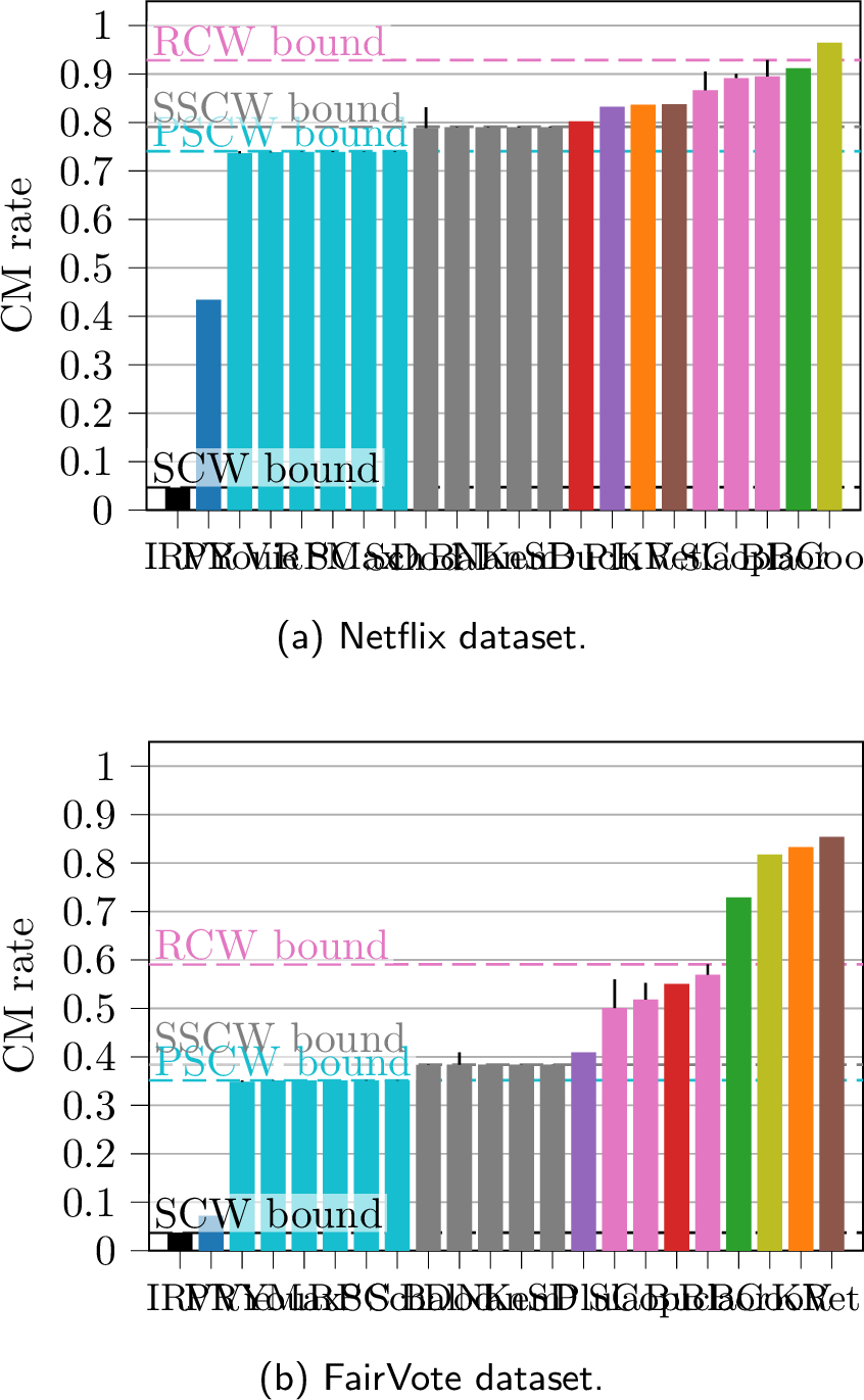
Figures [fig:netflix95cm95rate95bar95plot95more] and [fig:fairvote95cm95rate95bar95plot95more95rules] revisit Figures [fig:netflix95cm95rate95bar95plot] and [fig:fairvote95cm95rate95bar95plot]. They again report overall CM rates, but now include all values of \(m\), rather than being restricted to \(m \geq 5\). In addition, they incorporate the two voting rules analyzed only in the appendix, namely Split Cycle and Viennot.

First, we observe that for Slater and Copeland, the CM rates are less closely aligned with the RCW bound and with the CM rate of Black. This behavior was expected, since our theoretical results do not apply to Slater when \(m=3\), nor to Copeland when \(m \in \{3,4\}\).

Split Cycle empirically confirms its classification within the Maximin family.

The same observation holds for Viennot, and this case is particularly interesting. Indeed, Viennot shares the same critical concentration parameter as the other rules in the family, but not the same structural connection with the PSCW notion. This further supports the predictive power of the critical concentration parameter.

References↩︎

---

1. We adopt the terminology of [17], although the two rules coincide only when the number of voters is odd; in general, our definition matches the rule \(V\) of [22]. Our results apply to both.↩︎

2. For Kim–Roush, the original definition uses “strictly below” as here [14], whereas for Nanson it is “at most equal” [23]. This distinction does not affect our results.↩︎

3. We do not include the plurality-based analogue, IRV-Average, since it exhibits essentially the same behavior as IRV with respect to coalitional manipulation [5], [20].↩︎

4. Useless swaps also explain why it is NP-hard to determine the winner for the Dodgson rule [26].↩︎

5. The case \(d=e\) only matters when \(m=2\); for \(m\geq 3\), it can be omitted since it is implied by the case \(d\neq e\).↩︎

6. Note the importance of the assumption \(m \ge 3\) here: if \(m = 2\), candidates 2 and \(m\) coincide, and candidate 2 then receives \(\tfrac{1}{2}(1 - \theta) + \theta\) vetoes.↩︎