Self-conditioned Flow Map Language Models via Fixed-point Flows
July 01, 2026
Abstract
Self-conditioning is a core technique that enhances continuous flow-based language models, where the model learns to denoise generated text by conditioning on its own denoising estimate. While empirically successful, its performance improvements are poorly understood. Moreover, there is growing interest in the use of few-step generators based on flow maps, for which how to leverage self-conditioning is unclear. Here, we show that flow language models with self-conditioning solve a fixed-point iteration that bootstraps the performance of the learned denoiser. We use this viewpoint to formulate fixed-point flows, a two-dimensional class of self-conditioned flows, where the first dimension represents the flow process and the second represents the fixed-point iteration. We show that fixed-point flows define valid flow maps, and show that they can be distilled from self-conditioned flow models by compressing both fixed-point iterations and the flow process, the former with fixed-point distillation and the latter with flow map distillation. Our resulting flow map language model, FMLM\(^\star\), outperforms state-of-the-art self-conditioned models and few-step models in one- and few-step generation on OpenWebText.1
1 Introduction↩︎
Language models (LMs) based on continuous flows have recently emerged as a promising paradigm for non-autoregressive text generation [1]–[3]. By learning to denoise tokens in a continuous space, these models perform parallel iterative generation through a deterministic evolution driven by a velocity field. Importantly, such processes define a unique flow map, the solution operator that directly transports noise to data in as few as one function evaluation. This advantage has sparked recent breakthroughs on distillation of flow language models into flow map language models that are capable of generating text in one to few inference steps [1], [4], [5].
Recently, the performance of flow language models has improved through the incorporation of a self-conditioning mechanism [6]. Unlike in usual flow training, self-conditioned flow models learn to denoise an input by conditioning on its own denoising prediction. Then, during generation, they perform denoising at each flow timestep by conditioning on the previously denoised outcome. Self-conditioning has empirically proven very effective [7], [8], and has been widely adopted in the latest state-of-the-art flow language models [9]–[13]. Yet, despite its success, why self-conditioning leads to improvements remains poorly understood. Furthermore, it is unclear how to distill flows into flow maps under self-conditioning, as it introduces additional dependencies across generation timesteps.
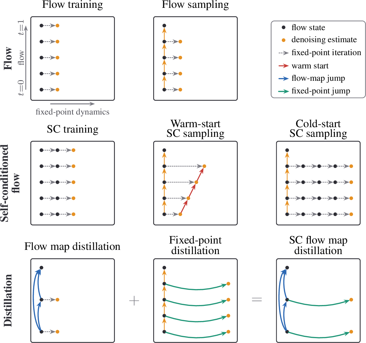
In this work, we introduce fixed-point flows, a mathematical framework for self-conditioned flows and their associated flow maps (1). Our key observation is that self-conditioned flow language models solve a fixed-point iteration that bootstraps the performance of learned denoising. With this insight, we characterize a two-dimensional class of self-conditioned flows, where the first dimension represents the original flow, and the second represents fixed-point iterations. We use this view to distill self-conditioned flow language models into flow maps by compressing both fixed-point iterations and flow, achieving state-of-the-art one- and few-step language modeling. Our main contributions are:
Fixed-point view of self-conditioning. We show that flow language models with self-conditioning implicitly learn a fixed-point iteration that refines the denoising estimate. We theoretically show that such behavior can emerge from self-conditioned training under a contractivity assumption.
Fixed-point flows and their flow maps. We introduce fixed-point flows, a formalization of self-conditioned flows. We show that fixed-point flows define a valid flow map, which can be learned by compressing both fixed-point iterations and flow with the respective few-step distillation objectives.
Empirical results. We distill self-conditioned flow language models into flow map language models, achieving state-of-the-art one- and few-step generation on OpenWebText. We also show that it is possible to distill self-conditioned models into self-conditioning-free ones without degradation.
2 Preliminary↩︎
2.0.0.1 Flow language models.
Let \(V\) be a vocabulary of tokens, and denote text data with length \(L\) by \({\boldsymbol{y}} = ({\boldsymbol{y}}^l)_{l=1}^L \in V^L\). The goal of language modeling is to learn the data distribution \(p({\boldsymbol{y}})\) so that we can draw a new text sample efficiently. Flow language models choose a continuous embedding \({\boldsymbol{y}}\mapsto {\boldsymbol{x}}\in\mathbb{R}^{L\times d}\) and a decoder \({\boldsymbol{x}}\mapsto {\boldsymbol{y}}\), and model the induced distribution \(p({\boldsymbol{x}})\) on the embedding space, generating \(\hat{{\boldsymbol{x}}}\sim p({\boldsymbol{x}})\) and then rounding into discrete language through \(\hat{{\boldsymbol{x}}}\mapsto \hat{{\boldsymbol{y}}}\).
To model the now-continuous data distribution \(p({\boldsymbol{x}})\), flow language models use flow matching over a stochastic interpolant [14], [15]. They specify a probability path \(p_t({\boldsymbol{x}}_t)\) over \(t\in[0,1]\) as the density of an interpolant \(I_t \mathrel{\vcenter{:}}= (1-t){\boldsymbol{x}}_0 + t{\boldsymbol{x}}_1\) between noise \({\boldsymbol{x}}_0\sim p_0\) and data \({\boldsymbol{x}}_1\sim p_1\). The path \(p_t\) admits a deterministic evolution equation that can be used to draw a sample \({\boldsymbol{x}}_t\sim p_t\) at inference time: \[\label{eq:flow95velocity} \dot{{\boldsymbol{x}}}_t = b_t({\boldsymbol{x}}_t),\quad b_t({\boldsymbol{x}}) = \mathbb{E}[{\boldsymbol{x}}_1-{\boldsymbol{x}}_0 \mid I_t = {\boldsymbol{x}}],\quad {\boldsymbol{x}}_0\sim p_0,\quad t\in[0,1],\tag{1}\] where \(b_t\) is the velocity field of the flow. If a model \(\hat{b}\) of the velocity is available, a sample \(\hat{{\boldsymbol{x}}}_1\sim p_1\) can be approximately drawn by numerically integrating 1 across a time grid \(0=t_0<...<t_N=1\). A simple choice for the integration is the forward Euler scheme: \[\label{eq:euler} \hat{{\boldsymbol{x}}}_{t_{i+1}} = \hat{{\boldsymbol{x}}}_{t_i} + (t_{i+1}-t_i)\hat{b}_{t_i}(\hat{{\boldsymbol{x}}}_{t_i}),\quad \hat{{\boldsymbol{x}}}_0\sim p_0.\tag{2}\] Instead of learning the velocity directly, it is more common in language modeling to learn the denoiser \(D_t\) [1], [10] which outputs the mean of clean data, and from which one can recover the velocity [15], [16]: \[\label{eq:denoiser} D_t({\boldsymbol{x}}) \mathrel{\vcenter{:}}= \mathbb{E}[{\boldsymbol{x}}_1\mid I_t={\boldsymbol{x}}],\quad b_t({\boldsymbol{x}}) = \frac{D_t({\boldsymbol{x}}) - {\boldsymbol{x}}}{1-t}.\tag{3}\] The ideal denoiser \(D\) can be learned in practice by solving a regression problem \(D = \mathop{\mathrm{argmin}}_{\hat{D}}\mathcal{L}(\hat{D})\) that predicts clean data by minimizing the following loss: \[\label{eq:denoiser95loss} \mathcal{L}(\hat{D}) \mathrel{\vcenter{:}}= \int_0^1 \mathbb{E}|\hat{D}_t(I_t) - {\boldsymbol{x}}_1|^2{\rm d}t.\tag{4}\] While we have used square loss above, our discussions and results readily transfer to the cross-entropy setting of [1], [7], [17]. With a learned denoiser \(\hat{D}\), generation can be done by turning it into an estimation of the velocity \(\hat{b}\) through 3 and then leveraging the forward Euler scheme 2 .
2.0.0.2 Flow map language models.
A key advantage of continuous flow for language modeling is that its deterministic generative process 1 driven by the velocity \(b_t\) defines a unique flow map \(X_{s,t}:\mathbb{R}^{L\times d}\to \mathbb{R}^{L\times d}\), the solution operator that transports a sample directly \({\boldsymbol{x}}_t=X_{s,t}({\boldsymbol{x}}_s)\) between any timesteps \((s,t)\in[0,1]^2\). It satisfies the following integral equation: \[\label{eq:flow95map} X_{s,t}({\boldsymbol{x}}_s) = {\boldsymbol{x}}_s + \int_s^t b_\tau({\boldsymbol{x}}_\tau)\,{\rm d}\tau.\tag{5}\] If available, a flow map allows for efficient few-step generation by sequentially evaluating \(\hat{{\boldsymbol{x}}}_{t_{i+1}} = X_{t_i,t_{i+1}}(\hat{{\boldsymbol{x}}}_{t_i})\) upon any grid \(0=t_0<...<t_N=1\), even one-step generation via \(\hat{{\boldsymbol{x}}}_1 = X_{0,1}(\hat{{\boldsymbol{x}}}_0)\).
Recent works have demonstrated that flow map language models can be learned by distilling the flow velocity learned by flow language models [1], [4], [5]. These methods leverage a set of mathematical relations between the flow velocity and the flow map [1], [18], which are derivable from the integral equation in 5 , and learn the flow map with respect to a given flow velocity to satisfy these relations.
3 Theoretical framework↩︎
In this section, we formalize self-conditioning and propose that it learns a fixed-point iteration which refines the denoising prediction. We then develop fixed-point flows, a framework for self-conditioned flows, along with the associated flow maps for few-step generation. Finally, we introduce distillation methods for turning self-conditioned flow language models into few-step language models.
3.1 Self-conditioned flow language models↩︎
Self-conditioning is a technique introduced in [6] where the denoiser learns to predict conditioned on its own denoising estimates. In these approaches, the model of the denoiser 3 takes an additional conditioning, \(\hat{D}_t({\boldsymbol{x}}, {\boldsymbol{z}})\), which effectively reduces to a usual denoiser model when \({\boldsymbol{z}}=\boldsymbol{0}\). The denoiser is trained using the following loss, where \(\mu\) is a choice of training-time distribution of \({\boldsymbol{z}}\): \[\label{eq:sc95loss} \mathcal{L}_\mu(\hat{D}) \mathrel{\vcenter{:}}= \int_0^1\mathbb{E}_{{\boldsymbol{x}}_0,{\boldsymbol{x}}_1}\mathbb{E}_\mu|\hat{D}_t(I_t, {\boldsymbol{z}}) - {\boldsymbol{x}}_1|^2{\rm d}t.\tag{6}\] A common choice of \(\mu\) is the mixture of delta peaks at zero \({\boldsymbol{z}}=\boldsymbol{0}\) and the model’s own denoising prediction \({\boldsymbol{z}} = \mathsf{sg}(\hat{D}_t(I_t, \boldsymbol{0}))\) where \(\mathsf{sg}\) is the stop-gradient operator. This leads to the following: \[\label{eq:sc95loss95decomposed} \mathcal{L}_\mu(\hat{D}) = \frac{1}{2}\int_0^1\mathbb{E}|\hat{D}_t(I_t, \boldsymbol{0}) - {\boldsymbol{x}}_1|^2{\rm d}t + \frac{1}{2}\int_0^1\mathbb{E}|\hat{D}_t(I_t, \mathsf{sg}(\hat{D}_t(I_t, \boldsymbol{0})))- {\boldsymbol{x}}_1|^2 {\rm d}t,\tag{7}\] where the first term is the usual denoising loss 4 , whereas the second term is a self-conditioned loss which encourages correcting an initial estimate by the model.
In general, the conditioning variable \({\boldsymbol{z}}\) in the training loss 6 does not change the learning target of the denoiser. This is because the Bayes-optimal prediction of \({\boldsymbol{x}}_1\) given an interpolant \(I_t\) is specified by the ideal denoiser, \(D_t(I_t)\) 3 , regardless of \({\boldsymbol{z}}\), assuming \({\boldsymbol{z}}\) does not leak additional information about \({\boldsymbol{x}}_1\) beyond what is available from \(I_t\), as in 7 . Thus, the objective trains the model to map every on-distribution conditioning \({\boldsymbol{z}}\) to the ideal denoising target. We provide a formal proof:
propositionoptimality Assume that \({\boldsymbol{z}}\perp {\boldsymbol{x}}_1\mid I_t\) for almost every \(t\), and assume all second moments are finite. Then every unrestricted population minimizer \(\bar{D}\) of 6 satisfies \[\bar{D}_t({\boldsymbol{x}},{\boldsymbol{z}}) = D_t({\boldsymbol{x}})\] almost surely under the law of \((I_t, {\boldsymbol{z}})\), for almost every \(t\).
A proof is in 6.1. In practice, training would not attain the minimum loss and the model would have dependence on \({\boldsymbol{z}}\). With the self-conditioned loss 7 , this can encourage a self-correcting behavior that produces an initial prediction and then pulls it closer to the Bayes-optimal prediction.
The generative process under self-conditioning is similar to that of 1 , evolving a sample \(\hat{{\boldsymbol{x}}}_{t_i}\) across a flow-time grid \(0=t_0<...<t_N=1\). Yet, the denoising estimate is also maintained and updated as \(\hat{{\boldsymbol{z}}}_{t_i}\) to condition and bootstrap the denoiser, altering the numerical integration scheme 2 as follows: \[\label{eq:sc95euler} \begin{align} \hat{{\boldsymbol{x}}}_{t_{i+1}} &= \hat{{\boldsymbol{x}}}_{t_i} + (t_{i+1} - t_i) \hat{b}_{t_i},\quad \hat{b}_{t_i} = \frac{\hat{{\boldsymbol{z}}}_{t_{i+1}} - \hat{{\boldsymbol{x}}}_{t_i}}{1-t_i},\quad \hat{{\boldsymbol{x}}}_0\sim p_0,\\ \hat{{\boldsymbol{z}}}_{t_{i+1}} &= \hat{D}_{t_i}(\hat{{\boldsymbol{x}}}_{t_i}, \hat{{\boldsymbol{z}}}_{t_i}),\quad \hat{{\boldsymbol{z}}}_0 = \boldsymbol{0}. \end{align}\tag{8}\] Intuitively, this creates an information sharing across flow timesteps via \(\hat{\boldsymbol{z}}\) on top of the flow state \(\hat{\boldsymbol{x}}\).
Although self-conditioning empirically leads to substantial improvements of flow language models [9]–[13], understanding of its mechanism is limited [6], [7], [19], [20]. Furthermore, since the self-conditioned velocity 8 is no longer autonomous on the flow state but now also coupled with the updates of the denoising estimates, it is unclear how to use it for few-step distillation, which relies on the existence of the flow map characterized as a purely integral solution of the flow velocity 5 .
3.2 Self-conditioning induces a fixed-point iteration↩︎
We present our key intuition that a self-conditioned denoiser, trained with 7 , learns to improve its own predictions, implementing an iteration that approximately converges toward the ideal denoiser.
Formally, a self-conditioned denoiser \(\hat{D}({\boldsymbol{x}},{\boldsymbol{z}})\), given a choice of flow timestep \(t\) and flow state \({\boldsymbol{x}}\), can be used to define the following iteration \({\boldsymbol{z}}^j\) for \(j = 0, 1,...\) that starts at some initialization \({\boldsymbol{z}}^0\): \[\label{eq:sc95map} {\boldsymbol{z}}^{j+1} = \hat{D}_t({\boldsymbol{x}}, {\boldsymbol{z}}^j).\tag{9}\] As the denoiser learns to correct its own prediction 7 , we posit that it characterizes a self-correcting process, eventually reaching a fixed point \({\boldsymbol{z}}^\star = \hat{D}_t({\boldsymbol{x}}, {\boldsymbol{z}}^\star)\) [21]. We could think of this fixed point as a self-corrected approximation of the Bayes-optimal prediction \(D_t({\boldsymbol{x}})\), since it is the learning target as shown in [prop:optimality]. We make this intuition precise with a series of theoretical results.
First, we recall the notion of a contraction, which suffices for convergence to a unique fixed point.
definitioncontraction A function \(f:\mathbb{R}^d\to \mathbb{R}^d\) is a contraction on a closed set \(O\subseteq \mathbb{R}^d\) with factor \(0\leq \eta<1\) if it satisfies \(f(O)\subseteq O\) and \(|f({\boldsymbol{z}}) - f({\boldsymbol{z}}')| \leq \eta |{\boldsymbol{z}}-{\boldsymbol{z}}'|\) for every \({\boldsymbol{z}},{\boldsymbol{z}}'\in O\).
By [prop:optimality], a perfect denoiser \(\bar{D}_t({\boldsymbol{x}},\cdot)\) with minimum loss maps directly to \(D_t({\boldsymbol{x}})\), making it a contraction with \(\eta=0\). When the denoiser \(\hat{D}\) is learned, it is not always guaranteed to be contractive. Yet, in 6.2, we show that optimizing self-conditioned loss leads to approximate contractivity. To simplify our analysis, we shall henceforth assume that the learned denoiser is contractive. This is in line with common assumptions in looped models [22]–[26] and supported by our results that self-conditioned models ELF [10] and LangFlow [9] approximate fixed-point iterations. We show:
propositionlearnedfixedpoint Fix \(t\), \({\boldsymbol{x}}\), and \(0\leq\eta < 1\). Assume that \(\hat{D}_t({\boldsymbol{x}}, \cdot)\) is a contraction on a nonempty closed set \(O\subseteq\mathbb{R}^{L\times d}\) with factor \(\eta\). Then, the iteration \({\boldsymbol{z}}^{j+1} = \hat{D}_t({\boldsymbol{x}}, {\boldsymbol{z}}^j)\) 9 from any \({\boldsymbol{z}}^0\in O\) satisfies the following properties:
It converges exponentially to a unique fixed point \({\boldsymbol{z}}^\star\in O\),
Its denoising error at any iteration \(j\geq 0\) is bounded as \[|{\boldsymbol{z}}^j - D_t({\boldsymbol{x}})| \leq |\hat{D}_t({\boldsymbol{x}},{\boldsymbol{z}}^0) - D_t({\boldsymbol{x}})| + \frac{\eta-\eta^j}{1-\eta} |{\boldsymbol{z}}^1 - {\boldsymbol{z}}^0|.\]
Its denoising error at the fixed point is bounded as \[|{\boldsymbol{z}}^\star - D_t({\boldsymbol{x}})| \leq |\hat{D}_t({\boldsymbol{x}},{\boldsymbol{z}}^0) - D_t({\boldsymbol{x}})| + \frac{\eta}{1-\eta} |{\boldsymbol{z}}^1 - {\boldsymbol{z}}^0|,\]
A proof is in 6.3. The result shows that the denoising loss at the initialization, together with the magnitude of the first iteration, controls the denoising error bound of multi-step iterations during inference up to the fixed point. It further shows that the error bound improves with iterations.
Having formulated the relationship between a self-conditioned denoiser \(\hat{D}\) and its fixed points for each pair of \(t\) and \({\boldsymbol{x}}\), it is convenient to think of a function that directly predicts the fixed point. We call such a function the fixed-point denoiser \(D^\star\), defined as follows for every \(t\in[0,1],{\boldsymbol{x}}\in\mathbb{R}^{L\times d}\): \[\label{eq:fp95denoiser} D_t^\star({\boldsymbol{x}}) \mathrel{\vcenter{:}}= {\boldsymbol{z}}^\star = \hat{D}_t({\boldsymbol{x}}, {\boldsymbol{z}}^\star).\tag{10}\] where \({\boldsymbol{z}}^\star\) is the unique fixed point of \(\hat{D}_t({\boldsymbol{x}}, \cdot)\). The fixed-point denoiser is a self-conditioning-free denoiser that behaves the same as the given self-conditioned denoiser run until convergence. Its ideal target under [prop:optimality] is the Bayes-optimal prediction \(D_t({\boldsymbol{x}})\), in which case we have \(D^\star=D\).
3.3 Fixed-point flows↩︎
In 3.1, we have seen that self-conditioned flow appears to involve two states: the flow state and the self-conditioning state. In 3.2, we have established that a self-conditioned denoiser induces a fixed-point iteration. Here, we propose to replace the self-conditioning state by its fixed point. Once this is done, the velocity depends only on the flow state, so it becomes an ordinary flow. We call this a fixed-point flow, and prove its fundamental properties as follows.
propositionfpflow Assume that, for every \(t\in[0,1)\) and \({\boldsymbol{x}}\), the self-conditioned denoiser \(\hat{D}_t({\boldsymbol{x}},\cdot)\) has a unique fixed point \(D^\star_t({\boldsymbol{x}}) = \hat{D}_t({\boldsymbol{x}},D^\star_t({\boldsymbol{x}}))\). Define the fixed-point velocity \[\label{eq:fp95velocity} b_t^\star({\boldsymbol{x}}) \mathrel{\vcenter{:}}= \frac{D_t^\star({\boldsymbol{x}}) - {\boldsymbol{x}}}{1-t},\quad t\in[0,1).\tag{11}\] Then \(b_t^\star\) depends only on \(t\) and \({\boldsymbol{x}}\), and therefore the dynamics \[\label{eq:fp95ode} \dot{{\boldsymbol{x}}}_t = b_t^\star({\boldsymbol{x}}_t)\tag{12}\] define an ordinary time-dependent ODE. Furthermore, when the fixed-point denoiser is Bayes optimal, \(D^\star=D\), the fixed-point velocity recovers the true velocity, \(b^\star = b\).
A proof is in 6.4. Equation 11 says that at each flow time, the self-conditioned denoiser \(\hat{D}\) runs fixed-point iteration 9 until convergence, and the fixed point modulates the flow via 11 . This suggests an Euler scheme for sampling \(\hat{{\boldsymbol{x}}}_1\sim p_1\) over a flow-time grid \(0=t_0<...<t_N=1\): \[\hat{{\boldsymbol{x}}}_{t_{i+1}} = \hat{{\boldsymbol{x}}}_{t_i} + (t_{i+1} - t_i) \frac{\hat{{\boldsymbol{z}}}_{t_i}^\star - \hat{{\boldsymbol{x}}}_{t_i}}{1-t_i},\] where each \(\hat{{\boldsymbol{z}}}_{t_i}^\star\) is obtained by solving an inner fixed-point iteration from an initialization \(\hat{{\boldsymbol{z}}}_{t_i}^0\): \[\label{eq:inner95fpi} \hat{{\boldsymbol{z}}}_{t_i}^{j+1} = \hat{D}_{t_i}(\hat{{\boldsymbol{x}}}_{t_i}, \hat{{\boldsymbol{z}}}_{t_i}^j).\tag{13}\] If the fixed-point iteration is run until convergence, how it is initialized must not affect the outcome. Therefore, a simple and valid approach is to always initialize with zero, \(\hat{{\boldsymbol{z}}}_{t_i}^0=\boldsymbol{0}\), which we call cold-start sampling of a fixed-point flow. On the other hand, choosing the right initialization can improve the efficiency of finding the fixed point. This can be done, for instance, with the fixed-point estimate of the previous flow timestep, \(\hat{{\boldsymbol{z}}}_{t_i}^0 = \hat{{\boldsymbol{z}}}_{t_{i-1}}^\star\). We call this warm-start sampling, and show:
propositionconvergence In the setting of [prop:learnedfixedpoint], if \(|{\boldsymbol{z}}^0-{\boldsymbol{z}}^\star|> \varepsilon\), then it is enough to take \[j\geq \frac{\log |{\boldsymbol{z}}^0 - {\boldsymbol{z}}^\star|/\varepsilon}{\log (1/\eta)}\] iterations to guarantee \(|{\boldsymbol{z}}^j-{\boldsymbol{z}}^\star| \leq \varepsilon\).
A proof is given in 6.5. The result shows that initializing closer to the fixed point improves convergence, which is the case for warm-start sampling if the fixed points are correlated locally in \(t\).
With this, we can view conventional self-conditioned generation in 8 as warm-start sampling that approximates fixed points with a single iteration, \(\hat{{\boldsymbol{z}}}_{t_i}^\star\approx \hat{D}_{t_i}(\hat{{\boldsymbol{x}}}_{t_i},\hat{{\boldsymbol{z}}}_{t_{i-1}}^\star)\). This implies that the coupling of flow state and self-conditioning state in 8 is not a defining property of self-conditioned flows, as it is merely a byproduct of warm starts, a sampling heuristic. We indeed find that cold-start sampling with sufficient fixed-point iterations can replace warm starts in ELF [10] and LangFlow [9].
Taking this idea further, we find that it is possible to take a self-conditioned flow model and turn it into a self-conditioning-free model by distilling the self-conditioned denoiser \(\hat{D}\) into the fixed-point denoiser \(D^\star\). This can be done, for instance, via the following fixed-point distillation loss: \[\mathcal{L}(D^\star) = \int_0^1 \mathbb{E}|D_t^\star(I_t) - {\boldsymbol{z}}^\star|^2\,{\rm d}t, \quad {\boldsymbol{z}}^\star = \hat{D}_t(I_t,{\boldsymbol{z}}^\star), \label{eq:fp-z}\tag{14}\] where the target \({\boldsymbol{z}}^\star\) is estimated by iterating \({\boldsymbol{z}}^{j+1}=\hat{D}_t(I_t,{\boldsymbol{z}}^j)\) from \({\boldsymbol{z}}^0=\boldsymbol{0}\). Any other fixed-point distillation method can be used instead of 14 , such as consistency distillation [27]. The resulting fixed-point velocity \(b^\star\) is autonomous, so its generation can use the usual Euler scheme 2 .
3.4 Fixed-point flow maps↩︎
In 3.3, we have formalized fixed-point flows, which express self-conditioned flows via ordinary velocity fields. We leverage this insight to define their associated flow maps, which allows us to design few-step distillation methods for self-conditioned flow language models.
propositionfpflowmap On any interval where the fixed-point flow ODE 12 has unique solutions, the fixed-point flow map, its solution operator \(X_{s,t}^\star({\boldsymbol{x}}_s) = {\boldsymbol{x}}_t\), satisfies \[\label{eq:fixedpointflowmap} X^\star_{s,t}({\boldsymbol{x}})={\boldsymbol{x}} + \int_s^t b_\tau^\star({\boldsymbol{x}}_\tau)\,{\rm d}\tau.\tag{15}\] Moreover, for \(0\leq s\leq u\leq t< 1\), \[\label{eq:fpfm-semigroup} X_{s,t}^\star = X_{u,t}^\star \circ X_{s,u}^\star.\tag{16}\]
A proof is in 6.6. The result shows that \(X^\star\) is a valid flow map and admits conditions such as 16 that can be leveraged to learn it through distillation from the velocity \(b_t^\star\). In order to learn the flow map, we parameterize it with a two-time denoiser \(\delta_{s,t}\) defined as follows [1], [28]: \[\label{eq:twotimedenoiser} \delta_{s,t}({\boldsymbol{x}}) \mathrel{\vcenter{:}}= {\boldsymbol{x}} + (1-s) v_{s,t}({\boldsymbol{x}}),\tag{17}\] where \(v_{s,t}\) is the average velocity from \(s\) to \(t\), defined as follows [18]: \[v_{s,t}({\boldsymbol{x}}) \mathrel{\vcenter{:}}= \frac{X_{s,t}^\star({\boldsymbol{x}}) - {\boldsymbol{x}}}{t-s},\quad v_{t,t}({\boldsymbol{x}})\mathrel{\vcenter{:}}= b_t^\star({\boldsymbol{x}}).\] Analogous to the relationship between the single-time denoiser and velocity, \(D_t^\star({\boldsymbol{x}}) = {\boldsymbol{x}} + (1-t)b_t^\star({\boldsymbol{x}})\), the two-time denoiser can be viewed as a single denoising step to the clean data domain. Its outputs are known to lie in a low-dimensional manifold [1], [28], making learning easier. We now show:
propositiontwotimedenoiser The two-time denoiser \(\delta_{s,t}\) satisfies the following properties:
For \(0\le s<t<1\), the flow map is recovered from \(\delta_{s,t}\) by \[\label{eq:fm-recovery} X_{s,t}^\star({\boldsymbol{x}}) = \frac{1-t}{1-s}{\boldsymbol{x}} + \frac{t-s}{1-s}\delta_{s,t}({\boldsymbol{x}}).\tag{18}\]
On the diagonal, \[\label{eq:fm-diagonal} \delta_{t,t}({\boldsymbol{x}})=D_t^\star({\boldsymbol{x}}).\tag{19}\]
For \(0\le s<u<t<1\), the semigroup condition 16 is equivalent to \[\label{eq:fm-semigroup} \delta_{s,t}({\boldsymbol{x}}) = \gamma \delta_{s,u}({\boldsymbol{x}}) + (1-\gamma)\delta_{u,t}(X_{s,u}^\star({\boldsymbol{x}})),\tag{20}\] where \(\gamma=\tfrac{(1-t)(u-s)}{(1-u)(t-s)}\in[0,1]\).
A proof is in 6.7. The result shows that learning the two-time denoiser yields the flow map, and that the two-time denoiser matches the fixed-point denoiser \(D^\star\) 10 on the diagonal \(s=t\), while satisfying a self-consistency criterion off the diagonal. These conditions lead to a learning objective:
propositiontwotimedenoisertraining Consider the population objective \[\label{eq:fp-distill} \mathcal{L}(\delta) = \mathbb{E}_{s,u,t,{\boldsymbol{x}}} |\delta_{s,t}({\boldsymbol{x}})-\mathsf{sg}(\mathcal{T}(\delta)_{s,u,t}({\boldsymbol{x}}))|^2 + \mathbb{E}_{t,{\boldsymbol{x}}} |\delta_{t,t}({\boldsymbol{x}})-D_t^\star({\boldsymbol{x}})|^2\tag{21}\] where \[\mathcal{T}(\delta)_{s,u,t}({\boldsymbol{x}}) := \gamma \delta_{s,u}({\boldsymbol{x}}) + (1-\gamma) \delta_{u,t}\bigl(X_{s,u}^\star({\boldsymbol{x}})\bigr).\]
Then the true two-time denoiser has zero loss. Conversely, any zero-loss solution satisfies the diagonal 19 and semigroup 20 conditions almost surely under the training distribution.
A proof is given in 6.8. The first loss term enforces the semigroup condition, and the second loss term anchors the diagonal to the fixed point \(D_t^\star(I_t) = {\boldsymbol{z}}^\star = \hat{D}_t(I_t,{\boldsymbol{z}}^\star)\). Evaluating the latter requires fixed points \({\boldsymbol{z}}^\star\), which we may make available in one of two ways: an offline route that first distills the fixed-point denoiser \(D^\star\) as a separate model via 14 , or an online route that performs two compressions in 14 and 21 jointly, estimating \({\boldsymbol{z}}^\star\) with a few iterations of \({\boldsymbol{z}}^{j+1} = \hat{D}_t(I_t,{\boldsymbol{z}}^j)\) from \({\boldsymbol{z}}^0=\boldsymbol{0}\). The online approach ultimately achieves \(\delta_{t,t}\approx D_t^\star\) without training a separate model.
4 Experiments↩︎
Through our experiments, we aim to answer the following key questions:
Do self-conditioned flow language models learn fixed-point iterations?
Is self-conditioned generation merely offering better initialization of fixed points?
Can we train self-conditioning-free flows competitive with self-conditioned ones?
Can we train a flow map language model that leverages self-conditioning?
4.0.0.1 Setup.
We conduct all experiments on the OpenWebText dataset [29], a standard corpus for language modeling, with a sequence length of 1024 tokens. We assess generation quality with generative perplexity (gPPL) [7], [30] measured with pretrained GPT-2 Large [31], together with average per-sample unigram entropy. We regard a model as strong only when its generations attain low gPPL while remaining close to the data entropy of 5.44 nats [1]. We use 256 generated samples for analysis (4.1) and 1024 for distillation (4.2). See 7 for more experimental details.
4.1 Analyzing self-conditioned flow language models↩︎
To answer whether self-conditioned denoisers induce fixed-point iterations (Q1) and whether the gains of self-conditioned sampling come from improved initialization of fixed-point iterations (Q2), we study ELF [10] and LangFlow [9] as representatives of self-conditioned flow language models on learned embeddings and one-hot token embeddings, respectively. We draw gPPL-entropy frontier curves [32] by sweeping sampling parameter \(\gamma\) for ELF and softmax temperature for LangFlow.
4.1.0.1 Self-conditioning induces a fixed-point iteration (Q1).
We first ask whether self-conditioned denoisers learn fixed-point iteration 9 . Following [27], we track relative distance to the fixed point, \(|{\boldsymbol{z}}^j - {\boldsymbol{z}}^\star|/|{\boldsymbol{z}}^\star|\), which equals one at \(j=0\) when cold-start sampling is used (\({\boldsymbol{z}}^0={\boldsymbol{0}}\)). To approximate \({\boldsymbol{z}}^\star\), we run 200 damped Picard iterations [33] with a fixed damping parameter \(0.3\) (see 7.1 for details). As shown in 2, the relative distance decays across flow time \(t\) for both models. This supports that the models have approximately learned a fixed point iteration as posited in 3.2.
We now ask whether the fixed-point iteration converges towards the ideal denoiser (3.2). As illustrated in 1, gPPL decreases as the number of fixed-point iterations increases on both ELF and LangFlow, whereas entropy remains stable near the data distribution (5.44 nats), showing that taking more steps toward the fixed point produces a better denoiser, agreeing with [prop:learnedfixedpoint].


Figure 2: Convergence towards the fixed point across fixed-point iterations..
| ELF (32 steps), # FPIs | \(1\) | \(2\) | \(3\) | \(4\) | \(5\) |
|---|---|---|---|---|---|
| gPPL \(\downarrow\) | 101.19 | 66.50 | 56.67 | 50.25 | 46.31 |
| entropy | 5.51 | 5.42 | 5.37 | 5.33 | 5.31 |
| LangFlow (64 steps), # FPIs | \(1\) | \(2\) | \(3\) | \(4\) | \(5\) |
| gPPL \(\downarrow\) | 77.26 | 57.99 | 52.63 | 49.37 | 47.27 |
| entropy | 5.49 | 5.42 | 5.40 | 5.38 | 5.36 |
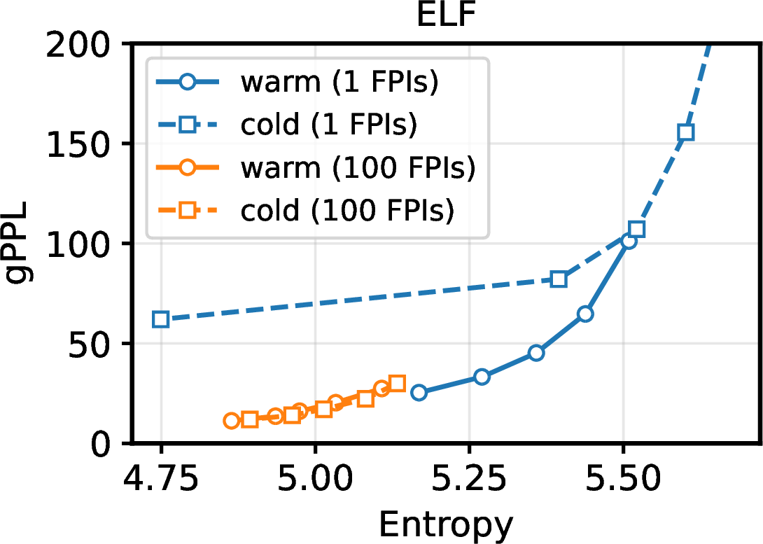
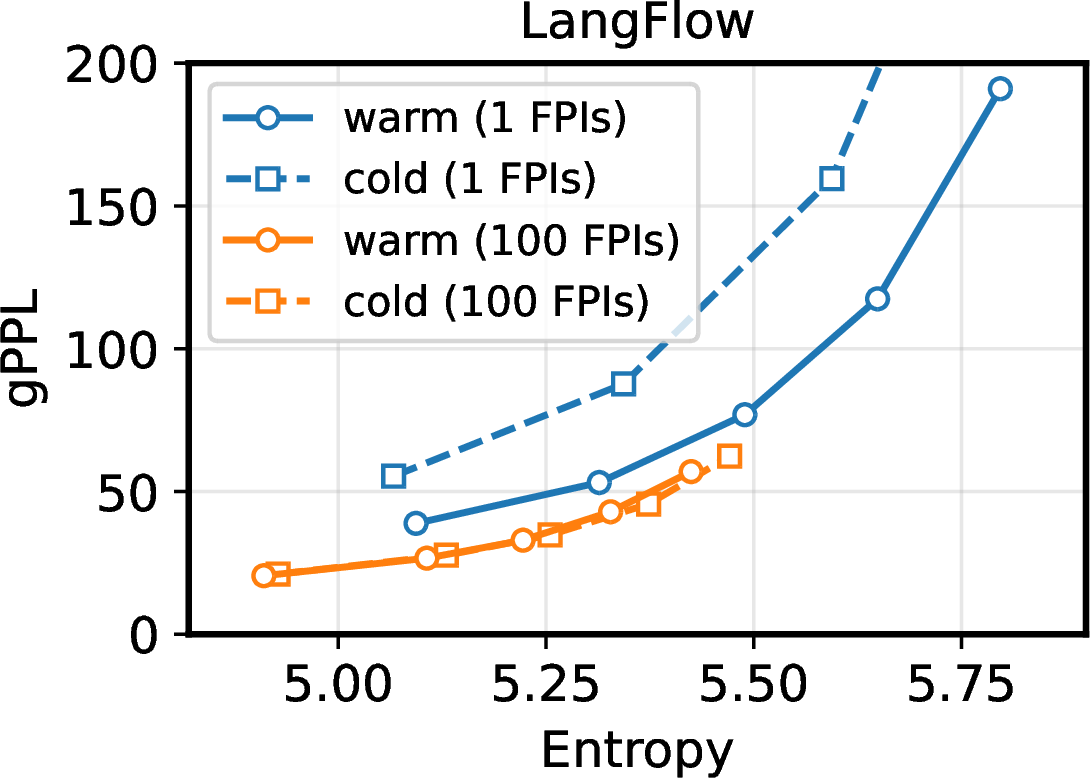
Figure 3: Warm-start and cold-start sampling with 1 and 100 fixed-point iterations..
4.1.0.2 Self-conditioned generation merely offers a better initialization (Q2).
In 3.3, we viewed conventional generation of self-conditioned flows as a warm-start sampling scheme that attempts to use a better initialization for the fixed-point iteration. Accordingly, we conjectured that cold-start sampling would reach a similar performance if sufficient iterations are used as it would eventually find the fixed point regardless of initialization. To validate this, we draw the gPPL–entropy frontier of each sampling scheme in 3. When we use a single fixed-point iteration, warm-start outperforms cold-start sampling, demonstrating that warm-start offers a good initialization around the fixed point. With 100 iterations, however, warm- and cold-start attain the same frontier, indicating that the choice of initialization has a negligible effect on generation once enough fixed-point iterations are run.
4.2 Distilling self-conditioning into fixed-point flow maps↩︎
To test self-conditioning-free distillation (Q3) and self-conditioned flow map distillation (Q4), we train ELF [10] as a teacher model, replacing its encoder with GPT-2 Large [31] for tokenizer-matched comparison with baselines.
| Step | Metric | Duo | MDLM | FMLM | DFM | FMLM\(^\star\) | |||
|---|---|---|---|---|---|---|---|---|---|
| 3-4 (lr)5-6 (lr)8-9 | DCD | Di4C | SDTT | Di4C | PSD | ESD | |||
| 1 | gPPL \(\downarrow\) | 5743.29 | 370.51 | 1260.86 | 1298.80 | 168.30 | 180.29 | 5.33 | 112.52 |
| entropy | 6.02 | 3.92 | 5.26 | 5.29 | 5.17 | 4.91 | 0.26 | 5.37 | |
| 2 | gPPL \(\downarrow\) | 891.16 | 210.22 | 877.22 | 758.23 | 133.29 | 152.83 | 108.91 | 94.74 |
| entropy | 5.41 | 4.63 | 5.34 | 5.35 | 5.25 | 5.03 | 5.15 | 5.45 | |
| 4 | gPPL \(\downarrow\) | 250.86 | 154.67 | 339.73 | 239.27 | 111.31 | 122.32 | 77.08 | 75.22 |
| entropy | 5.37 | 4.85 | 5.38 | 5.40 | 5.26 | 5.10 | 5.27 | 5.41 | |

4.2.0.1 Self-conditioning is removable (Q3).
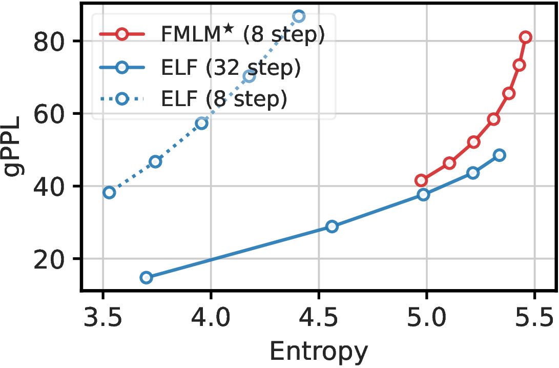
We find that, given a self-conditioned denoiser \(\hat{D}\) (ELF in our case), we can learn its associated fixed-point denoiser \(D^\star\) 10 through fixed-point distillation, which yields fixed-point velocity 11 , a self-conditioning-free model. Herein, we consider CDEQ [27], an existing fixed-point distillation method. Using the method, we distill the ELF teacher into a self-conditioning-free model ELF\(^\star\), with implementation details provided in 7. We compare 8-step generation performance of ELF\(^\star\) against 32-step generation of the teacher with gPPL-entropy frontier curves. As in 4, ELF\(^\star\) matches the teacher’s frontier, confirming that self-conditioning is removable via fixed-point distillation without degrading quality.
4.2.0.2 Self-conditioning is distillable into a flow map (Q4).
Finally, we ask whether self-conditioning can be leveraged to train a few-step flow map. To this end, we distill the self-conditioned ELF teacher into a self-conditioned flow map language model FMLM\(^\star\), parameterized by the two-time denoiser \(\delta_{s,t}\) 17 . Following the offline route proposed in 3.4, we take the fixed-point denoiser ELF\(^\star\) as teacher and learn its associated fixed-point flow map with the semigroup distillation objective 21 . As illustrated in 5, FMLM\(^\star\) with 8 generation steps approaches the 32-step frontier of the self-conditioned teacher ELF.
We then compare FMLM\(^\star\) in one-step and few-step generation settings on OpenWebText against recent few-step distillation baselines: discrete diffusion models Duo with DCD [30], MDLM with SDTT [34], and both with Di4C [35], and continuous flow map language models FMLM [1] and DFM [5], reporting gPPL and entropy. As shown in 2, FMLM\(^\star\) attains the best gPPL among baselines that preserve data-level entropy (5.44 nats) in the one- and few-step regimes, advancing the state-of-the-art under a matched sampling budget. Qualitative samples can be found in 8.
| Step | Metric | # FPIs for online distillation | Offline | |||||
|---|---|---|---|---|---|---|---|---|
| 3-8 | 1 | 2 | 3 | 5 | 9 | 17 | ||
| 1 | gPPL \(\downarrow\) | 176.31 | 141.06 | 134.49 | 121.44 | 116.74 | 118.26 | 112.52 |
| entropy | 5.47 | 5.42 | 5.42 | 5.41 | 5.39 | 5.38 | 5.37 | |
| 2 | gPPL \(\downarrow\) | 149.51 | 114.85 | 109.29 | 99.98 | 97.44 | 98.37 | 94.74 |
| entropy | 5.53 | 5.50 | 5.49 | 5.49 | 5.47 | 5.47 | 5.45 | |
| 4 | gPPL \(\downarrow\) | 120.35 | 90.75 | 88.20 | 80.27 | 79.87 | 80.05 | 75.22 |
| entropy | 5.46 | 5.45 | 5.46 | 5.46 | 5.45 | 5.45 | 5.41 | |
| Training times | 18h | 18h | 19h | 20h | 24h | 33h | 82h | |
To reduce training cost, we also consider online distillation, which avoids training a separate fixed-point denoiser (ELF\(^\star\) in our case). FMLM\(^\star\) instead distills directly from the self-conditioned teacher (ELF) using a fixed number of cold-start fixed-point iterations at each training step. As shown in 3, its performance saturates around 9 FPIs, and the resulting online-distilled FMLM\(^\star\) achieves competitive quality at approximately \(0.3\times\) the training cost of offline-distilled FMLM\(^\star\). Together, these results show that self-conditioning can be leveraged to build a state-of-the-art few-step flow map through either two-stage offline distillation or cheaper one-stage online distillation (Q4).
5 Conclusion↩︎
We demonstrated that the self-conditioned flow language model implicitly learns a fixed-point iteration that refines its own denoising estimate, approximately converging toward the ideal denoiser. Such convergence is provable under a contractivity assumption, and we observe it empirically in existing self-conditioned models. Based on this viewpoint, we proposed fixed-point flows, a class of self-conditioned flows organized along two axes: the flow over time and the fixed-point iteration at each flow time, which also offers an understanding of conventional self-conditioned sampling as a single-step warm-started fixed-point iteration. Building on fixed-point flows, we proposed a method to distill self-conditioned flows into a flow map language model FMLM\(^\star\) that enables few-step generation while inheriting the excellent performance of self-conditioned flows. On OpenWebText, FMLM\(^\star\) achieves state-of-the-art one- and few-step generation under matched sampling budgets.
5.0.0.1 Limitations and future work.
We restrict our flow map learning to the distillation setting which requires a separate teacher model (e.g., ELF or ELF\(^\star\)). A promising next step is extending to self-distillation that only uses data supervision, simultaneously learning the self-conditioned denoiser, fixed-point denoiser, and two-time denoiser in a single model. In addition, we have limited our scope to text data, although our formulation is general and would apply to other modalities such as graphs, images, and videos. Understanding self-conditioning in these modalities would prove interesting.
6 Proofs↩︎
6.1 Proof of Proposition [prop:optimality]↩︎
Proof. Fix \(t\) for which the conditional independence assumption holds, and write \[D\mathrel{\vcenter{:}}= D_t(I_t), \qquad U\mathrel{\vcenter{:}}= \hat{D}_t(I_t,{\boldsymbol{z}}).\] Then \[{\boldsymbol{x}}_1-U=({\boldsymbol{x}}_1-D)+(D-U).\] Squaring and taking expectations gives \[\mathbb{E}|{\boldsymbol{x}}_1-U|^2 = \mathbb{E}|{\boldsymbol{x}}_1-D|^2 + \mathbb{E}|U-D|^2 + 2\mathbb{E}\langle {\boldsymbol{x}}_1-D,D-U\rangle.\] The cross term vanishes. Indeed, \[\mathbb{E}[{\boldsymbol{x}}_1-D\mid I_t,{\boldsymbol{z}}] = \mathbb{E}[{\boldsymbol{x}}_1\mid I_t,{\boldsymbol{z}}]-D_t(I_t).\] By the conditional independence assumption, \[\mathbb{E}[{\boldsymbol{x}}_1\mid I_t,{\boldsymbol{z}}] = \mathbb{E}[{\boldsymbol{x}}_1\mid I_t] = D_t(I_t).\] Hence \[\mathbb{E}[{\boldsymbol{x}}_1-D\mid I_t,{\boldsymbol{z}}]=0,\] and therefore \[\mathbb{E}\langle {\boldsymbol{x}}_1-D,D-U\rangle=0.\] Thus \[\mathbb{E}|\hat{D}_t(I_t,{\boldsymbol{z}})-{\boldsymbol{x}}_1|^2 = \mathbb{E}|{\boldsymbol{x}}_1-D_t(I_t)|^2 + \mathbb{E}|\hat{D}_t(I_t,{\boldsymbol{z}})-D_t(I_t)|^2.\] The first term does not depend on \(\hat{D}_t\). The second term is minimized exactly when \[\hat{D}_t(I_t,{\boldsymbol{z}})=D_t(I_t)\] almost surely under the law of \((I_t,{\boldsymbol{z}})\). Integrating over \(t\) gives the claim. ◻
6.2 Proof of approximate contractivity↩︎
We show that learning the self-conditioned objective leads to an approximate notion of contractivity.
Definition 1 (A simplified self-conditioned regression.). Let \(O\subseteq\mathbb{R}^d\) be a nonempty and closed set, let \(Z\sim \mu\) with \(\mu(O) = 1\), let \(X\in\mathbb{R}^d\) be fixed, and let \(f:\mathbb{R}^d\to\mathbb{R}^d\) be a continuous function. For some \(0 < p < 1\), we define the following self-conditioned regression objective: \[\label{eq:simplified95self95conditioned95regression} \mathcal{L}(f)\mathrel{\vcenter{:}}= p\mathbb{E}|f(Z) - X|^2 + (1-p)\mathbb{E}|f(f(Z)) - X|^2.\tag{22}\]
This is a simplification of our problem setting in 3.1. Taking \(p=1/2\), \(f = \hat{D}_t(I_t,\cdot)\), and \(X = D_t({\boldsymbol{x}})\) (the Bayes-optimal prediction target; [prop:optimality]), for fixed \(t\in[0,1]\) and \({\boldsymbol{x}}\), we recover a practical learning scenario for self-conditioned language models similar to 7 .
Let us fix
a scale \(w>0\),
a factor \(0\leq\eta<1\),
a tolerance \(r>0\),
and a failure probability \(0<\varepsilon<1\).
Let us assume: \[\label{eq:approx95contractivity95assumption} \bar{B}(X,r) \subseteq O,\quad 2r\leq \eta w,\quad \mathcal{L}(f)\leq \min\{p, 1-p\}\varepsilon r^2.\tag{23}\] Define \[A \mathrel{\vcenter{:}}= \{{\boldsymbol{z}}\in O:|f({\boldsymbol{z}}) - X|\leq r\}.\]
The following lemmas show that a sufficiently small loss yields a closed, high-probability set \(A\) that is contractive with factor \(\eta\) above the scale \(w\), and approximately forward-invariant under the training distribution with leakage at most \(\varepsilon\). Intuitively, the first term in the self-conditioned loss makes the set \(A\) high-probability under \(\mu\), whereas the second term makes \(f(Z)\) remain in \(A\) for most \(Z\sim \mu\).
Lemma 1 (Closedness and approximate forward invariance). \(A\) is a closed subset of \(\mathbb{R}^d\). Furthermore, \(f(A)\subseteq O\), and it holds that \[\mu(A\cap f^{-1}(A)) \geq 1-\varepsilon.\] In particular, \(\mu(A)\geq 1-\varepsilon\) and \[\mu(\{{\boldsymbol{z}}\in A: f({\boldsymbol{z}})\notin A\}) \leq \varepsilon.\]
Proof. The closed Euclidean ball \(\bar{B}(X, r)\) is closed. Since \(f\) is continuous, \[f^{-1}(\bar{B}(X, r))\] is closed. Therefore, \[A = O\cap f^{-1}(\bar{B}(X, r))\] is closed because \(O\) is closed.
For every \({\boldsymbol{z}}\in A\), we have, by definition, \[|f({\boldsymbol{z}}) - X| \leq r.\] Hence \[f({\boldsymbol{z}})\in \bar{B}(X, r).\] By assumption 23 , \[f(A)\subseteq O.\]
Define the initial and self-conditioned errors \[e_1({\boldsymbol{z}})\mathrel{\vcenter{:}}= |f({\boldsymbol{z}})-X|,\quad e_2({\boldsymbol{z}})\mathrel{\vcenter{:}}= |f(f({\boldsymbol{z}}))-X|.\] and define \[G \mathrel{\vcenter{:}}= \{{\boldsymbol{z}}\in O: e_1({\boldsymbol{z}})\leq r \text{ and } e_2({\boldsymbol{z}})\leq r\}.\] The condition \(e_1({\boldsymbol{z}})\leq r\) is exactly \({\boldsymbol{z}}\in A\).
Moreover, as we have seen, \(e_1({\boldsymbol{z}})\leq r\) implies \(f({\boldsymbol{z}})\in O\). Therefore, \[e_2({\boldsymbol{z}})\leq r\] is equivalent to \[f({\boldsymbol{z}})\in A.\] Consequently, \[G = A\cap f^{-1}(A).\]
On the complement \(G^c\), at least one of the inequalities \[e_1({\boldsymbol{z}}) \leq r,\quad e_2({\boldsymbol{z}}) \leq r\] fails.
If \(e_1({\boldsymbol{z}}) > r\), then \[p e_1({\boldsymbol{z}})^2 > pr^2 \geq \min\{p, 1-p\}r^2.\] If \(e_2({\boldsymbol{z}}) > r\), then \[(1-p) e_2({\boldsymbol{z}})^2 > (1-p)r^2 \geq \min\{p, 1-p\}r^2.\] Thus, for every \({\boldsymbol{z}}\notin G\), \[pe_1({\boldsymbol{z}})^2 + (1-p)e_2({\boldsymbol{z}})^2 \geq \min\{p, 1-p\}r^2.\] Equivalently, \[\boldsymbol{1}({\boldsymbol{z}}\notin G) \leq \frac{pe_1({\boldsymbol{z}})^2 + (1-p)e_2({\boldsymbol{z}})^2}{\min\{p, 1-p\}r^2}.\] Taking expectation with respect to \(Z\sim \mu\), \[\mu(G^c)\leq \frac{\mathbb{E}[pe_1({\boldsymbol{z}})^2 + (1-p)e_2({\boldsymbol{z}})^2]}{\min\{p, 1-p\}r^2} = \frac{\mathcal{L}(f)}{\min\{p, 1-p\}r^2}.\] By assumption 23 , \[\mu(G^c)\leq \varepsilon.\] Therefore, \[\mu(G)\geq 1 - \varepsilon.\] Since \(G = A\cap f^{-1}(A)\), \[\mu(A\cap f^{-1}(A))\geq 1 - \varepsilon.\] This implies \(\mu(A)\geq 1 - \varepsilon\) because \(A\cap f^{-1}(A)\subseteq A\).
It also implies \[\mu(A\setminus f^{-1}(A))\leq \varepsilon,\] because the event \[A\setminus f^{-1}(A) = \{{\boldsymbol{z}}\in A:f({\boldsymbol{z}})\notin A\}\] is contained in \(G^c\). ◻
Lemma 2 (Approximate contractivity). For every \({\boldsymbol{z}},{\boldsymbol{z}}'\in A\) satisfying \(|{\boldsymbol{z}} - {\boldsymbol{z}}'| \geq w\), one has \[|f({\boldsymbol{z}}) - f({\boldsymbol{z}}')|\leq \eta |{\boldsymbol{z}} -{\boldsymbol{z}}'|.\]
Proof. Take arbitrary \({\boldsymbol{z}},{\boldsymbol{z}}'\in A\). By definition of \(A\), \[|f({\boldsymbol{z}}) - X| \leq r,\quad |f({\boldsymbol{z}}') - X| \leq r.\] By the triangle inequality, \[|f({\boldsymbol{z}}) - f({\boldsymbol{z}}')| \leq |f({\boldsymbol{z}}) - X| + |f({\boldsymbol{z}}') - X| \leq 2r.\] By assumption, \[2r \leq \eta w.\] Therefore, whenever \(|{\boldsymbol{z}} - {\boldsymbol{z}}'| \geq w\), \[|f({\boldsymbol{z}}) - f({\boldsymbol{z}}')| \leq 2r \leq \eta w \leq \eta|{\boldsymbol{z}} - {\boldsymbol{z}}'|.\] Hence \[|f({\boldsymbol{z}}) - f({\boldsymbol{z}}')|\leq \eta |{\boldsymbol{z}} -{\boldsymbol{z}}'|\] for every pair \({\boldsymbol{z}},{\boldsymbol{z}}'\in A\) separated by at least \(w\). ◻
6.3 Proof of Proposition [prop:learnedfixedpoint]↩︎
We first show a useful lemma.
Lemma 3. Let \(f:\mathbb{R}^d\to\mathbb{R}^d\) be a contraction on a nonempty closed set \(O\subseteq\mathbb{R}^d\) with factor \(0\leq\eta<1\). Then, there is a unique fixed point \({\boldsymbol{z}}^\star\in O\), to which the iteration \[{\boldsymbol{z}}^{j+1} = f({\boldsymbol{z}}^j)\] from any \({\boldsymbol{z}}^0\in O\) converges exponentially. Furthermore, the following holds for any finite \(j\geq k\geq 0\): \[|{\boldsymbol{z}}^j - {\boldsymbol{z}}^k| \leq \frac{\eta^k-\eta^j}{1-\eta} |{\boldsymbol{z}}^1 - {\boldsymbol{z}}^0|.\] Similarly, the following holds: \[|{\boldsymbol{z}}^\star - {\boldsymbol{z}}^k| \leq \frac{\eta^k}{1-\eta} |{\boldsymbol{z}}^1 - {\boldsymbol{z}}^0|.\]
Proof. Because \(O\) is a closed subset of \(\mathbb{R}^d\), it is complete. The map \(f\) maps \(O\) into itself and is a contraction on \(O\). Therefore, by the Banach fixed-point theorem, \(f\) has a unique fixed point \({\boldsymbol{z}}^\star\in O\), and the iterates converge to it.
A geometric convergence bound follows directly from the contraction property: \[|{\boldsymbol{z}}^{j+1}-{\boldsymbol{z}}^\star| = |f({\boldsymbol{z}}^j) - f({\boldsymbol{z}}^\star)| \le \eta |{\boldsymbol{z}}^j-{\boldsymbol{z}}^\star|.\] Repeating this inequality gives \[\label{eq:geometric95convergence} |{\boldsymbol{z}}^j-{\boldsymbol{z}}^\star| \le \eta^j|{\boldsymbol{z}}^0-{\boldsymbol{z}}^\star|.\tag{24}\]
For \(j\geq k\geq 0\), telescoping gives \[{\boldsymbol{z}}^j - {\boldsymbol{z}}^k = \sum_{i=k}^{j-1}({\boldsymbol{z}}^{i+1} - {\boldsymbol{z}}^i).\] Taking norms and applying the triangle inequality, \[\label{eq:telescoping95norm} |{\boldsymbol{z}}^j - {\boldsymbol{z}}^k| = \left|\sum_{i=k}^{j-1}({\boldsymbol{z}}^{i+1} - {\boldsymbol{z}}^i)\right| \leq \sum_{i=k}^{j-1} |{\boldsymbol{z}}^{i+1} - {\boldsymbol{z}}^i|.\tag{25}\] Each increment can be bounded using the contraction property: \[|{\boldsymbol{z}}^{i+1} - {\boldsymbol{z}}^i| = |f({\boldsymbol{z}}^i) - f({\boldsymbol{z}}^{i-1})| \leq \eta |{\boldsymbol{z}}^i - {\boldsymbol{z}}^{i-1}|.\] Repeating this inequality gives \[|{\boldsymbol{z}}^{i+1} - {\boldsymbol{z}}^i| \leq \eta^i |{\boldsymbol{z}}^1 - {\boldsymbol{z}}^0|.\] Applying this in 25 , \[|{\boldsymbol{z}}^j - {\boldsymbol{z}}^k| \leq \sum_{i=k}^{j-1} \eta^i |{\boldsymbol{z}}^1 - {\boldsymbol{z}}^0|.\] The geometric sum is \[\sum_{i=k}^{j-1} \eta^i = \frac{\eta^k-\eta^j}{1-\eta}.\] Thus, \[|{\boldsymbol{z}}^j - {\boldsymbol{z}}^k| \leq \frac{\eta^k-\eta^j}{1-\eta} |{\boldsymbol{z}}^1 - {\boldsymbol{z}}^0|.\] Finally, since \({\boldsymbol{z}}^j\to{\boldsymbol{z}}^\star\), continuity of the norm gives \[|{\boldsymbol{z}}^\star-{\boldsymbol{z}}^k| = \lim_{j\to\infty}|{\boldsymbol{z}}^j-{\boldsymbol{z}}^k|.\] Therefore, \[|{\boldsymbol{z}}^\star-{\boldsymbol{z}}^k| \leq \lim_{j\to\infty} \frac{\eta^k-\eta^j}{1-\eta} |{\boldsymbol{z}}^1-{\boldsymbol{z}}^0| = \frac{\eta^k}{1-\eta} |{\boldsymbol{z}}^1-{\boldsymbol{z}}^0|.\] ◻
Proof. Since \(\hat{D}_t({\boldsymbol{x}},\cdot)\) is a contraction on \(O\), by applying 3 to it, we have that \({\boldsymbol{z}}^j\) converges exponentially to a unique fixed point \({\boldsymbol{z}}^\star\in O\). Furthermore, we have \[\label{eq:difference95bound} |{\boldsymbol{z}}^j - {\boldsymbol{z}}^k| \leq \frac{\eta^k-\eta^j}{1-\eta} |{\boldsymbol{z}}^1 - {\boldsymbol{z}}^0|,\quad |{\boldsymbol{z}}^\star - {\boldsymbol{z}}^k| \leq \frac{\eta^k}{1-\eta} |{\boldsymbol{z}}^1 - {\boldsymbol{z}}^0|.\tag{26}\] By the triangle inequality, \[|{\boldsymbol{z}}^j - D_t({\boldsymbol{x}})| \leq |{\boldsymbol{z}}^j - \hat{D}_t({\boldsymbol{x}},{\boldsymbol{z}}_0)| + |\hat{D}_t({\boldsymbol{x}},{\boldsymbol{z}}_0) - D_t({\boldsymbol{x}})|.\] By the definition of the iteration, \[|{\boldsymbol{z}}^j - D_t({\boldsymbol{x}})| \leq |{\boldsymbol{z}}^j - {\boldsymbol{z}}^1| + |\hat{D}_t({\boldsymbol{x}},{\boldsymbol{z}}_0) - D_t({\boldsymbol{x}})|.\] Using the first part of 26 with \(k=1\), \[|{\boldsymbol{z}}^j - D_t({\boldsymbol{x}})| \leq |\hat{D}_t({\boldsymbol{x}},{\boldsymbol{z}}_0) - D_t({\boldsymbol{x}})| + \frac{\eta-\eta^j}{1-\eta} |{\boldsymbol{z}}^1 - {\boldsymbol{z}}^0|.\] Applying the same argument, with the second part of 26 , \[|{\boldsymbol{z}}^\star - D_t({\boldsymbol{x}})| \leq |\hat{D}_t({\boldsymbol{x}},{\boldsymbol{z}}_0) - D_t({\boldsymbol{x}})| + \frac{\eta}{1-\eta} |{\boldsymbol{z}}^1 - {\boldsymbol{z}}^0|.\] ◻
6.4 Proof of Proposition [prop:fpflow]↩︎
Proof. By definition, \(D_t^\star({\boldsymbol{x}})\) is obtained by solving the inner self-conditioning fixed-point problem at the pair \((t,{\boldsymbol{x}})\). Hence, after taking the fixed point, there is no remaining conditioning variable \({\boldsymbol{z}}\). Therefore \[b_t^\star({\boldsymbol{x}}) = \frac{D_t^\star({\boldsymbol{x}})-{\boldsymbol{x}}}{1-t}\] is a function only of \(t\) and \({\boldsymbol{x}}\).
The sampling dynamics are therefore the ordinary ODE \[\dot{\boldsymbol{x}}_t=b_t^\star({\boldsymbol{x}}_t).\]
When the fixed point matches the Bayes-optimal denoiser, \(D^\star=D\), then by 1 , we have that \[b_t^\star({\boldsymbol{x}}) = \frac{D_t({\boldsymbol{x}})-{\boldsymbol{x}}}{1-t} = b_t({\boldsymbol{x}}).\] Therefore, the fixed-point velocity recovers the true velocity. ◻
6.5 Proof of Proposition [prop:convergence]↩︎
Proof. From the geometric convergence bound 24 in 3, \[|{\boldsymbol{z}}^j - {\boldsymbol{z}}^\star| \leq \eta^j |{\boldsymbol{z}}^0 - {\boldsymbol{z}}^\star|.\] In the nontrivial case \(|{\boldsymbol{z}}^0-{\boldsymbol{z}}^\star|> \varepsilon\), it is enough to require \[\eta^j|{\boldsymbol{z}}^0 - {\boldsymbol{z}}^\star| \leq \varepsilon.\] Taking logarithms and using \(\log\eta<0\) gives \[j\geq \frac{\log |{\boldsymbol{z}}^0 - {\boldsymbol{z}}^\star|/\varepsilon}{\log (1/\eta)}.\] ◻
6.6 Proof of Proposition [prop:fpflowmap]↩︎
Proof. Since 12 is an ODE, it defines the flow map \(X_{s,t}^\star({\boldsymbol{x}}_s)={\boldsymbol{x}}_t\) wherever the ODE solution is unique. Uniqueness also gives the composition law: evolving from \(s\) to \(t\) is the same as first evolving from \(s\) to \(u\), and then from \(u\) to \(t\). Thus \[X_{s,t}^\star = X_{u,t}^\star\circ X_{s,u}^\star.\] ◻
6.7 Proof of Proposition [prop:twotimedenoiser]↩︎
Proof. First, by definition, \[\delta_{s,t}({\boldsymbol{x}}) = {\boldsymbol{x}}+(1-s)v_{s,t}({\boldsymbol{x}}).\] Therefore \[v_{s,t}({\boldsymbol{x}}) = \frac{\delta_{s,t}({\boldsymbol{x}})-{\boldsymbol{x}}}{1-s}.\] Substituting this into \[X_{s,t}^\star({\boldsymbol{x}}) = {\boldsymbol{x}}+(t-s)v_{s,t}({\boldsymbol{x}})\] gives \[X_{s,t}^\star({\boldsymbol{x}}) = {\boldsymbol{x}}+\frac{t-s}{1-s}\bigl(\delta_{s,t}({\boldsymbol{x}})-{\boldsymbol{x}}\bigr).\] Rearranging gives \[X_{s,t}^\star({\boldsymbol{x}}) = \frac{1-t}{1-s}{\boldsymbol{x}} + \frac{t-s}{1-s}\delta_{s,t}({\boldsymbol{x}}),\] which is 18 .
For the diagonal identity, \[\delta_{t,t}({\boldsymbol{x}}) = {\boldsymbol{x}}+(1-t)b_t^\star({\boldsymbol{x}}).\] Since \[b_t^\star({\boldsymbol{x}})=\frac{D_t^\star({\boldsymbol{x}})-{\boldsymbol{x}}}{1-t},\] we get \[\delta_{t,t}({\boldsymbol{x}})=D_t^\star({\boldsymbol{x}}),\] which is 19 .
It remains to prove the semigroup identity. Let \[{\boldsymbol{z}}:=X_{s,u}^\star({\boldsymbol{x}}) = \frac{1-u}{1-s}{\boldsymbol{x}} + \frac{u-s}{1-s}\delta_{s,u}({\boldsymbol{x}}).\] Using 18 , \[X_{s,t}^\star({\boldsymbol{x}}) = \frac{1-t}{1-s}{\boldsymbol{x}} + \frac{t-s}{1-s}\delta_{s,t}({\boldsymbol{x}}),\] \[X_{u,t}^\star({\boldsymbol{z}}) = \frac{1-t}{1-u}{\boldsymbol{z}} + \frac{t-u}{1-u}\delta_{u,t}({\boldsymbol{z}}).\] Since the semigroup property 16 holds, \[X_{s,t}^\star({\boldsymbol{x}})=X_{u,t}^\star(X_{s,u}^\star({\boldsymbol{x}}))=X_{u,t}^\star({\boldsymbol{z}}).\] Substituting the expression for \({\boldsymbol{z}}=X_{s,u}^\star({\boldsymbol{x}})\) into the right-hand side gives \[\begin{align} X_{s,t}^\star({\boldsymbol{x}}) &= \frac{1-t}{1-u}\left(\frac{1-u}{1-s}{\boldsymbol{x}}+\frac{u-s}{1-s}\delta_{s,u}({\boldsymbol{x}})\right) + \frac{t-u}{1-u}\delta_{u,t}({\boldsymbol{z}}) \\ & = \frac{1-t}{1-s}{\boldsymbol{x}} + \frac{(1-t)(u-s)}{(1-u)(1-s)}\delta_{s,u}({\boldsymbol{x}}) + \frac{t-u}{1-u}\delta_{u,t}({\boldsymbol{z}}). \end{align}\] and canceling the common \({\boldsymbol{x}}\)-term gives \[\frac{t-s}{1-s}\delta_{s,t}({\boldsymbol{x}}) = \frac{(1-t)(u-s)}{(1-u)(1-s)}\delta_{s,u}({\boldsymbol{x}}) + \frac{t-u}{1-u}\delta_{u,t}({\boldsymbol{z}}).\] Multiplying by \((1-s)/(t-s)\), we obtain \[\delta_{s,t}({\boldsymbol{x}}) = \frac{(1-t)(u-s)}{(1-u)(t-s)} \delta_{s,u}({\boldsymbol{x}}) + \frac{(1-s)(t-u)}{(1-u)(t-s)} \delta_{u,t}({\boldsymbol{z}}).\] Define \[\gamma = \frac{(1-t)(u-s)}{(1-u)(t-s)}.\] Then \[1-\gamma = \frac{(1-s)(t-u)}{(1-u)(t-s)}.\] Therefore \[\delta_{s,t}({\boldsymbol{x}}) = \gamma \delta_{s,u}({\boldsymbol{x}}) + (1-\gamma)\delta_{u,t}\bigl(X_{s,u}^\star({\boldsymbol{x}})\bigr).\]
Conversely, if this identity for \(\delta\) holds, then applying 18 to both sides gives \[X_{s,t}^\star({\boldsymbol{x}})=X_{u,t}^\star(X_{s,u}^\star({\boldsymbol{x}})).\] Thus the two identities are equivalent. ◻
6.8 Proof of Proposition [prop:twotimedenoisertraining]↩︎
Proof. By the two-time denoiser identities 19 and 20 , the true two-time denoiser \(\delta\) satisfies \[\delta_{t,t}({\boldsymbol{x}})=D_t^\star({\boldsymbol{x}})\] and \[\delta_{s,t}({\boldsymbol{x}}) = \gamma \delta_{s,u}({\boldsymbol{x}}) + (1-\gamma) \delta_{u,t}\bigl(X_{s,u}^\star({\boldsymbol{x}})\bigr).\] Therefore both squared-error terms in \(\mathcal{L}(\delta)\) are zero, and hence \[\mathcal{L}(\delta)=0.\]
Conversely, suppose \(\mathcal{L}(\delta)=0\). Since \(\mathcal{L}\) is a sum of nonnegative squared norms, each squared norm must vanish almost surely under its corresponding training distribution. The diagonal term gives \[\delta_{t,t}({\boldsymbol{x}})=D_t^\star({\boldsymbol{x}})\] almost surely. The semigroup term gives \[\delta_{s,t}({\boldsymbol{x}})=\mathcal{T}(\delta)_{s,u,t}({\boldsymbol{x}})\] almost surely. Substituting the definition of \(\mathcal{T}\), this becomes \[\delta_{s,t}({\boldsymbol{x}}) = \gamma \delta_{s,u}({\boldsymbol{x}}) + (1-\gamma) \delta_{u,t}\bigl(X_{s,u}^\star({\boldsymbol{x}})\bigr)\] almost surely. Thus any zero-loss solution satisfies the diagonal and semigroup consistency identities on the training distributions. ◻
7 Experiment Details↩︎
7.1 Analysis details↩︎
In 4.1 (2), we employ damped Picard iterations [33] to approximate the fixed point and update \({\boldsymbol{z}}^j\) with 200 iterations. The damped iteration is formulated as \({\boldsymbol{z}}^{j+1} = \alpha {\boldsymbol{z}}^{j} + (1-\alpha) \hat{D}_{t}({{\boldsymbol{x}}}_{t}, {\boldsymbol{z}}^{j})\), where \(\alpha\) is a damping hyperparameter. To find the fixed point at each timestep, we run this process for 200 iterations with \(\alpha = 0.3\).
For the analysis with generation performances ([tab:refinement,fig:warm_vs_cold_j8]), to ensure a fair comparison with the baseline self-conditioning, we utilize a standard Picard iteration (i.e., \(\alpha = 0.0\)) except for the runs with 100 iterations. For the 100-iteration runs, we retain the damped Picard with \(\alpha = 0.3\). For the sampling hyperparameters, we set the self-conditioning guidance weight in ELF [10] to \(w=1\).
7.2 Self-conditioning-free model details↩︎
We realize the fixed-point denoiser \(D^\star\) 10 as a self-conditioning-free model, ELF\(^\star\), by distilling a frozen self-conditioned ELF teacher \(\hat{D}\) [10] with consistency deep equilibrium (CDEQ) distillation [27]. The distillation compresses the fixed-point iteration 9 into a single forward that predicts its limit \({\boldsymbol{z}}^\star\), so the resulting model matches the converged self-conditioned denoiser without iterating at inference.
7.2.0.1 Architecture.
ELF [10] conditions on the flow time \(t\) through a bank of four learned prefix tokens, prepended to the latent sequence, to which an embedding of \(t\) is added; the self-conditioning guidance weight enters through a second such bank. Following this design, to let the student track progress along the iteration, we condition it on a consistency time \(\tau\) which represents the progress of fixed-point iteration in the same manner: we append a parallel bank of four phase tokens that carry an embedding of \(\tau\). We zero-initialize both the phase token bank and the \(\tau\)-embedder output, so the phase pathway is initially inert and the warm-started student nearly reproduces the teacher.
7.2.0.2 Training.
Following [27], at each step, we run the fixed-point iteration 9 at the training interpolant, \({\boldsymbol{z}}^{j+1}=\hat{D}_t({\boldsymbol{x}},{\boldsymbol{z}}^j)\), from the cold start \({\boldsymbol{z}}^0={\boldsymbol{0}}\) for \(K\) Anderson-accelerated steps, giving a detached trajectory \({\boldsymbol{z}}^0,\dots,{\boldsymbol{z}}^K\) whose last iterate we treat as the fixed point \({\boldsymbol{z}}^\star\). We assign iterate \({\boldsymbol{z}}^j\) a consistency time \(\tau_j=\varepsilon+(1-e^{-\rho j})(T-\varepsilon)\) with \(\tau_0=\varepsilon\), and let \(c_{\mathrm{skip}}(\tau)=(\tau-\varepsilon)/(T-\varepsilon)\) and \(c_{\mathrm{out}}(\tau)=1-c_{\mathrm{skip}}(\tau)\). The student predicts a consistency function \(g_j=c_{\mathrm{skip}}(\tau_j)\,{\boldsymbol{z}}^j+c_{\mathrm{out}}(\tau_j)\,P_j\), where \(P_j\) is a closed-form two-point Anderson combination (mixing \(1.0\)) of two phase-conditioned student passes. At the cold-start phase \(\tau_0\), we have \(c_{\mathrm{skip}}=0\), so \(g_j\) collapses to the bare network prediction, which is exactly what inference evaluates. We train \(g_j\) with a global term anchoring it to the equilibrium and a local term enforcing consistency with the previous phase, \(\mathcal{L}=\lambda_1|g_j-{\boldsymbol{z}}^\star|^2+(1-\lambda_1)|g_j-\mathsf{sg}(g_{j-1})|^2\), where the earlier-phase prediction is stop-gradient, and we retain the teacher’s decoder head [10].
We use \(K=20\) teacher iterations with Anderson history \(3\), mixing \(0.9\), and regularization \(10^{-4}\); a schedule with \(\varepsilon=0.002\), \(T=5.0\), \(\rho=0.3\); and loss weight \(\lambda_1=0.8\). Because the consistency weighting leaves the cold-start phase weakly supervised, with probability \(0.25\) we regress the cold-start point \(\tau_0\) directly onto \({\boldsymbol{z}}^\star\). The remaining optimization follows the teacher’s recipe (7.3).
7.2.0.3 Inference.
At inference, ELF\(^\star\) takes a single forward per flow step with a zero self-conditioning slot fixed at the cold-start phase \(\tau_0\), and carries no self-conditioning across flow steps. Its velocity is therefore autonomous, so generation uses the standard Euler scheme 2 .
7.3 Self-conditioning flow map details↩︎
7.3.0.1 Architecture.
We parameterize the two-time denoiser \(\delta_{s,t}\) 18 by conditioning the ELF backbone on both the source time \(s\) and the target time \(t\). We reuse ELF’s existing bank of flow-time prefix tokens, assigning half to the target \(t\) and half to the source \(s\) through the shared time-embedder; this introduces no new parameters and reduces to the single-time ELF denoiser on the diagonal \(s=t\), realizing the diagonal condition \(\delta_{s,s}=D^\star_s\) 19 by construction.
7.3.0.2 Training.
Each training step samples times \(0\le s\le u\le t\le 1\) and splits the batch per example into diagonal (\(s=t\)) and off-diagonal rows. Following 21 , diagonal rows regress \(\delta_{t,t}\) onto the fixed-point denoiser \(D^\star_t\). Off-diagonal rows regress \(\delta_{s,t}\) onto the semigroup teacher \(\bar{\delta}_{s,t}\), which we build from two stop-gradient passes of the current student, \(\delta_{s,u}\) and \(\delta_{u,t}\), chained through the midpoint state \(X^\star_{s,u}\) 18 by the convex weight \(\gamma\) 20 ; here \(u\) is the midpoint of \(s\) and \(t\) in the percentile parameterization. Following [1], we draw a diagonal row with probability \(0.5\) and pin a fraction \(1/32\) of the off-diagonal rows to the boundary \((s,t)=(0,1)\) to cover full one-step jumps. The times follow the teacher’s training-time marginal, a logit-normal distribution with \((\mu,\nu)=(-1.5,0.8)\). A single student forward at \((s,t)\) then carries the gradient, and we minimize the per-branch mean-squared error with equal weights.
The self-conditioned teacher is steered by a self-conditioning guidance weight \(w\) [10], which we hold fixed within each training example. We sample a single \(w\) per example, from the same log-uniform range \([0.5,5.0]\) used in ELF training, and feed that one value to every model call that enters its loss: the teacher passes that form the diagonal target \(D^\star_t\), the two student passes that form the off-diagonal semigroup target, and the graded student forward. Sharing one \(w\) across both branches and across teacher and student keeps the targets at a common guidance level, so the student learns a single \(w\)-conditioned flow map; at inference, \(w\) is likewise fixed across all steps and swept to trace the gPPL-entropy frontier.
The offline and online routes of 3.4 differ only in how the diagonal target \(D^\star_t\) is supplied. The two-stage FMLM\(^\star\) (offline) uses the separately distilled ELF\(^\star\) (7.2) as the teacher, which already returns \(D^\star_t\) in a single forward. The one-stage online FMLM\(^\star\) instead uses the self-conditioned ELF teacher and forms the target on the fly, cold-starting the iteration \({\boldsymbol{z}}^{j+1}=\hat{D}_t({\boldsymbol{x}},{\boldsymbol{z}}^j)\) at \({\boldsymbol{z}}^0={\boldsymbol{0}}\), running a fixed number of Picard refinements, and reading out \(D^\star_t\) with one final self-conditioned pass; the refinement count is the “# FPIs” in 3, where more iterations sharpen the target at a higher training cost.
For distillation in 4.2, we use ELF-B as the teacher model. To ensure tokenizer consistency with the baselines, we train a variant of ELF-B using the GPT-2 tokenizer. Specifically, we replace its original T5 text encoder [36] with the last hidden states of a pretrained GPT-2 Large model [31]. Aside from this modification, we strictly follow the original ELF architecture and train this variant using the identical hyperparameters.
We follow the hyperparameter settings of the original ELF model. Both models are trained for 5 epochs with a global batch size of 512 using 8 NVIDIA B200 GPUs. We employ a combination of Muon optimizers with a peak learning rate of 0.002, incorporating a learning rate warmup over the first 0.5 epochs. Additionally, we apply an exponential moving average (EMA) with a decay rate of 0.9999 and use the EMA checkpoint for inference.
7.3.0.3 Inference.
To report the gPPL and entropy for the two- and four-step FMLM\(^\star\) ([tab:onestep,tab:nrefinemaps]), we utilize \(\gamma\)-sampling [1], [37], [38] with \(\gamma = 0.75\) and \(1.0\), respectively.
8 Qualitative results↩︎
We provide generation samples from the FMLM\(^\star\) model. The one-step, two-step, and four-step samples are shown in 6, 7, and 8, respectively.
None
Figure 6: A sample generated by FMLM\(^\star\) with one-step decoding..
None
Figure 7: A sample generated by FMLM\(^\star\) with two-step decoding..
None
Figure 8: A sample generated by FMLM\(^\star\) with four-step decoding..
References↩︎
Code is available at https://github.com/Ugness/self-conditioned-fmlm.↩︎
Equal contribution \(^\dagger\) Equal advising↩︎