LUMA: Benchmarking Segmentation via a Lightweight Universal Mask Adapter
July 01, 2026
Abstract
Comparing transformer backbones for image segmentation is confounded: each is paired with a different decoder, recipe, and pretraining, so reported differences rarely reflect the backbone itself. We introduce the Lightweight Universal Mask Adapter(LUMA), a lightweight, backbone-agnostic mask-transformer head that treats any backbone as a black-box feature extractor, letting a set of queries read from its features through cheap cross-attention. LUMA matches the accuracy of EoMT, the state-of-the-art efficient ViT-segmenter, at lower cost, while attaching unchanged to isotropic, hierarchical, convolutional, and mixture-of-experts backbones alike. Holding this head fixed, we benchmark 20 backbones, 11 pretraining schemes and a range of resolutions on ADE20K and Cityscapes under one modern recipe. We find that “efficient” token mixers fail to deliver efficiency even at the high resolutions that motivate them, with plain ViT holding the throughput Pareto–front at every resolution. Additionally, the pretraining objective, not the architecture, the lever the field has tuned hardest, governs segmentation quality.
1 Introduction↩︎
Modern image segmentation is built on the mask transformer framework [1], [2], where a set of learnable queries is matched against the features of a pretrained backbone and decoded into a mask and class per segment. Many efforts have since optimized the mask-based segmentation-decoder [3]–[6]. Recently, EoMT [7] showed that this task-specific decoder part of the pipeline is largely unnecessary for plain ViT [8]. With a strong pretraining, the ViT backbone’s own self-attention can process the queries directly. Thus, in modern pipelines, most of the compute sits in the ViT backbone, for which decade of work has now gone into optimizing: efficient and linear attention [9]–[11], hierarchical and windowed token mixers [12], [13], convolutional hybrids [14]–[17], and state-space models [18]; almost all of these justified by efficiency at high resolution. This invites the question: Is the common backbone architecture of ViT itself necessary, or do pretraining and scale dominate dense transfer, and we can thus reap the efficiency gains of efficient backbones?
Answering this requires comparing backbones on equal footing: One segmentation head, that attaches to any backbone, adds only little compute, and reaches state-of-the-art accuracy. Trained with one training recipe, with only the backbone varying, so that measured differences reflect the architecture rather than the surrounding apparatus. Existing comparisons do not meet this bar, as each backbone is typically paired with its own decoder, recipe, pretraining, and resolution [19], [20] and the heavy task-specific decoders that dominate the leaderboard confound the backbone with the capacity of the head itself [2], [21]. EoMT, sporting only a very lightweight mask-head, is the natural fair instrument, but its efficiency comes from concatenating the queries into the token sequence and processing them with the backbone’s own attention, which presumes global attention, reach-in access to the block internals, and a constant token width. It is therefore a plain-ViT method by construction, and cannot be attached to the very backbones we wish to study.
We close this gap with the Lightweight Universal Mask Adapter(LUMA), a lightweight, efficient segmentation head that treats the backbone as a black-box feature extractor. Rather than inserting queries into the token stream, LUMA keeps them in a separate side stream and lets them read from each tapped block’s patch features through a lightweight cross-attention block, reusing the backbone’s own feed-forward layers, so the queries inherit any width schedule. The backbone runs exactly as it would on its own, so the identical head attaches unchanged to isotropic, hierarchical, windowed, convolutional, and mixture-of-experts backbones alike. This decoupling also yields a result complementary to EoMT’s: Queries need not live inside the backbone’s attention at all, as a minimal external read recovers the accuracy at lower cost, which is precisely what frees us from the global-attention and shared-width assumptions.
With LUMA held fixed as a fair measuring stick, we conduct a controlled study of 20 vision transformer backbones, 11 pretraining schemes and a range of input resolutions on ADE20K [22] and Cityscapes [23], all under a single modern segmentation recipe. This lets us disentangle, for the first time under one modern protocol, how segmentation quality is governed by the backbone architecture, by the pretraining objective, and by resolution.
Our dominant finding concerns the very property these architectures are designed for. “Efficient” token mixers exist to escape the \(\mathcal{O}(T^2)\) token scaling of attention, a cost that is negligible at the short sequences of \(224\) px classification but should dominate at the \(512\)–\(1024\) px resolutions segmentation tasks use. Nonetheless, even without FlashAttention, the plain ViT holds the throughput Pareto–front, with efficient variants competitive only in memory. The accuracy side tells the same story, as differences from architecture largely vanish once every backbone hosts the same head, with a few sequence-length-bound mixers (Linformer [9], Synthesizer [24], MLP-Mixer [25]) failing to generalize to high resolution; a failure classification benchmarks never expose. In line with this, ImageNet top-1 accuracy is an unreliable predictor of segmentation quality across backbones. Orthogonally, the pretraining objective is decisive: dense objectives transfer robustly while supervised pretraining is a categorical outlier despite competitive classification accuracy.
In summary: (1) we introduce LUMA, a lightweight, backbone-agnostic mask transformer head that matches EoMT’s accuracy at lower cost while attaching unchanged to any token mixer, and show that queries need not be embedded in the backbone’s attention to do so; (2) using LUMA as a fixed instrument, we present the broadest fair benchmark of transformer backbones for segmentation to date, spanning 20 architectures, 11 pretraining schemes, and multiple resolutions under one recipe; (3) using it to disentangle architecture, pretraining, and resolution, we show that token-mixer design is a weak lever for dense prediction while the pretraining objective and plain scale are the strong ones, and that the plain ViT remains the backbone of choice.
2 Related Work↩︎
Segmentation with Transformers. Segmentation was initially dominated by CNNs, whose feature maps naturally yield dense, pixel-level predictions [26]–[28]. After the introduction of ViT [8], custom variants were developed specifically for segmentation [29]. A key development was the MaskFormer family [1], [2], which reframed segmentation as predicting a set of masks with associated class labels rather than classifying each pixel independently, and now underpins most state-of-the-art segmenters [3]–[5]. To utilize plain ViTs for segmentation, heavy pixel decoders were appended after the backbone [1], [3], [6], [30] and adapters reaching into its intermediate stages were introduced [2], [4], [21]. Recently, EoMT [7] showed that this machinery is largely unnecessary, repurposing the backbone’s own self-attention as the adapter to match MaskFormer-like region queries to image patches with only a lightweight mask module on top. Our LUMA continues this trend toward minimal segmenters, generalizing the EoMT setup beyond plain self-attention backbones to arbitrary token mixers, while keeping the head lightweight via only a few cross-attention layers.
Vision Transformer Backbones. The \(\mathcal{O}(T^2)\) scaling of self-attention in the number of tokens \(T\) makes the plain ViT [8] costly at the high resolutions segmentation demands, motivating a wide range of architectural modifications. Following the taxonomy of efficient transformer variants by [31], we benchmark low-rank attention (Linformer [9], Nyströmformer [11]), sparse attention (Swin [12], Wave-ViT [32]), fixed attention (Synthesizer [24]), kernel attention (Poly-SA [33], Hydra [34]), and hybrid attention (EfficientViT [16], Next-ViT [17], CvT [14], ResT [15], CoaT [35]); non-attention token mixers that replace attention entirely (MLP-Mixer [25], EfficientMod [10], FocalNet [36]); and models that modify the feed-forward block (Switch [37], HiViT [38]). For a broader overview of efficient transformers, we refer to [31], [39], [40].
Pretraining Strategies. Backbones are typically initialized from weights pretrained on a large dataset, and this choice of pretraining objective strongly affects downstream segmentation quality [41]. Traditionally, computer vision pretraining relied on large-scale supervised image classification [42]–[44], for which the dominant transformer recipes are DeiT [45] and DeiT III [46]. More recent objectives move beyond labels: image–text contrastive learning (CLIP [47], SigLIP [48], AIMv2 [49]), masked image modeling (MAE [50], BEiT-3 [51], EVA-02 [52]), the self-distillation family of DINO [53]–[55], self-supervised segmentation pretraining SAM [13] and recently the joint-embedding predictive I-JEPA [56]. We benchmark representatives of all families.
Benchmarking Segmentation. Several prior works benchmark components of the segmentation pipeline in isolation. [57], [58] compare CNN and transformer backbones, but predate modern mask-based segmenters and large-scale pretraining. [19] benchmark segmentation decoders while holding the backbone fixed, and [41] benchmark pretraining objectives using a lightweight linear-probe adapter. BoB [20] benchmarks backbones for multiple tasks, including segmentation, but they conflate architecture and pretraining differences, as “different pretraining algorithms were trained on different datasets and architectures” [20]. [59] target the few-shot setting, and [60] evaluate segmentation robustness. In contrast, we benchmark 20 backbone architectures, using the same pretraining setup, and 8 pretraining schemes under a single modern recipe, plugging each into LUMA, a lightweight, backbone-agnostic, MaskFormer-based segmentation head. This lets us disentangle the contributions of architecture, pretraining, and resolution under a fair, modern segmentation protocol.
3 Method↩︎
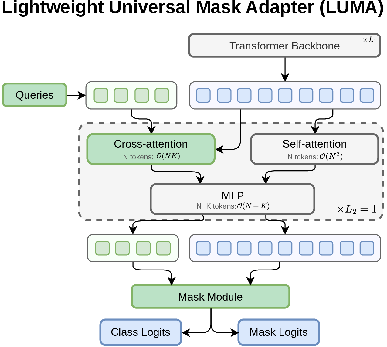
Our goal is to benchmark a broad range of transformer backbones for image segmentation on equal footing. This requires a segmentation head that (i) attaches to any backbone without architecture-specific surgery, (ii) adds as little compute as possible so that measured differences reflect the backbone rather than the head, and (iii) reaches the accuracy of state-of-the-art mask transformers. No existing design satisfies all three at once: heavy task-specific decoders inflate and confound the head, while the recent EoMT [7] is lightweight but tightly coupled to the plain ViT and cannot be applied to most backbones we wish to study. We therefore introduce the Lightweight Universal Mask Adapter(LUMA), a minimal head that treats the backbone as a black-box feature extractor and lets a small set of learnable queries read from its features through a single lightweight cross-attention layer. LUMA matches EoMT in accuracy, and efficiency, but crucially applies to any backbone family.
3.1 Preliminaries↩︎
Modern segmentation models follow the mask transformer framework [1], [2]: a set of \(K\) learnable queries \(\mathbf{Q}_0 = \{\mathbf{q}_i \in \mathbb{R}^{D}\}_{i=1}^{K}\) each learn to represent a single segment (a thing instance or a stuff class). The queries are refined against image features and then decoded into a class label and a binary mask per query. Class logits \(\mathbf{c}_i \in \mathbb{R}^{C}\) are obtained with a linear layer, and mask logits are obtained by passing each query through an MLP to a mask embedding \(\hat{\mathbf{q}}_i\) and taking its dot product with high-resolution image features. By assigning each ground-truth segment to a unique query and supervising both predictions, the model learns segmentation in a task-agnostic way. State-of-the-art models such as Mask2Former [2] refine queries with a heavy stack of multi-scale deformable cross-attention and self-attention, which heavily increase the head’s cost.
A transformer backbone maps an image \(\mathbf{I}\in\mathbb{R}^{3\times H\times W}\) to a sequence of feature tokens through \(L\) blocks. Backbones differ widely in how they do this: plain ViTs [8] keep a constant token count and embedding dimension and use global self-attention; hierarchical backbones such as Swin [12] downsample across stages, grow the embedding dimension, and use windowed or local attention; and recent state-space and convolutional hybrids replace attention entirely [17], [18], [36]. A backbone-agnostic head must cope with all of these without assuming any particular attention mechanism, token layout, or dimension schedule.
3.2 EoMT and the backbone-coupling problem↩︎
EoMT [7] removes the decoder altogether. It concatenates the \(K\) queries into the token sequence after the first \(L_1 = L - L_2\) blocks, and lets the final \(L_2\) out of the \(L\) backbone blocks process queries and patch tokens jointly through the ViT’s own multi-head self-attention. During training, intermediate masks are predicted before each of these blocks and used to mask the query-to-patch attention, mimicking the masked cross-attention of Mask2Former; a mask-annealing schedule then phases this masking out so that inference needs no masking at all. The result is elegant and efficient: the head is little more than a handful of extra tokens and a small mask module.
This efficiency, however, is purchased with three implicit assumptions about the backbone: (1) Global attention. Because the queries are appended to the token sequence and must attend to all patches, the backbone’s attention must be global; windowed or neighborhood attention would confine each query to a single window. (2) Accessible, uniform attention internals. To inject the attention mask, EoMT re-implements the block’s attention and reaches into its projections, heads, and normalization. This ties the head to the plain ViT block and also prevents the backbone from running its own fused attention kernel in the final blocks. In short, EoMT is a plain-ViT-only method by construction. It is therefore unsuitable as a benchmarking instrument, since most of the backbones we want to compare cannot host it at all.
3.3 LUMA: a Lightweight Universal Mask Adapter↩︎
The key idea behind LUMA is to make the queries backbone-agnostic, by decoupling them from the backbone’s token-mixing mechanism. Instead of inserting queries into the token stream and relying on the backbone’s attention to mix them with image features, LUMA keeps the queries in a separate side stream and gives them a cheap, explicit way to read from the backbone’s patch features. The backbone is run exactly as it would be on its own, block by block, and is never modified, re-implemented, or even aware of the queries. An overview is shown in 1.
Query side stream. Let \(\mathbf{X}^{i}\) denote the patch features produced by backbone block \(i\), and let \(\mathbf{Q}^{i}\) denote the query states, initialized from a learnable embedding \(\mathbf{Q}^{L_1}\). For each such block \(i\), LUMA updates the queries in two steps. First, a single lightweight cross-attention layer lets the queries read from the current patch features, which supply the keys and values. Second, the queries are passed through that block’s own feed-forward sub-layer, reusing the backbone’s MLP with its existing weights: \[\begin{align} \begin{aligned} \tilde{\mathbf{Q}}^{i} & = \mathbf{Q}^{i} + \texttt{LS}(\texttt{XAttn}(\mathbf{Q}^{i},\,\mathbf{X}^{i})), \\ \mathbf{Q}^{i+1} & = \tilde{\mathbf{Q}}^{i} + \texttt{MLP}_i\!\big(\texttt{Norm}_i(\tilde{\mathbf{Q}}^{i})\big), \end{aligned} \label{eq:luma-update} \end{align}\tag{1}\] where \(\texttt{XAttn}\) is cross-attention and \(\texttt{LS}\) is a per-channel LayerScale [61]. Together these form the only new parameters LUMA introduces at block \(i\). The normalization \(\texttt{Norm}_i\) and feed-forward layer \(\texttt{MLP}_i\) are block \(i\)’s own, applied to the queries with exactly the weights used for the patch tokens. The patch stream is left untouched, \(\mathbf{X}^{i+1} = \texttt{Block}_i(\mathbf{X}^{i})\), so the queries influence the backbone only by reading from it through 1 , never by entering its self-attention.
Reusing the backbone’s feed-forward sub-layer also dictates how LUMA handles a changing token dimension. Because the queries are processed by block \(i\)’s MLP and cross-attend to its patch features, \(\mathbf{Q}^{i}\) and \(\mathbf{X}^{i}\) must share the same width. For plain ViTs this holds trivially, but hierarchical backbones change their internal dimension between stages through an explicit mechanism (e.g.the projection within patch merging [12]). Rather than add a projection of our own, which would be redundant and a source of architecture-specific tuning, LUMA routes the queries through the same dimension-changing operation the backbone applies to its tokens. The queries thus inherit the backbone’s width schedule for free and stay dimension-aligned with the patch features at every block, regardless of how that width changes.
Masked attention. A central mechanism in EoMT is masked attention during training, which constrains each query to attend only within its own predicted segmentation mask, together with a mask-annealing schedule that gradually phases this masking out so that inference can run without it. This machinery exists because queries and patches share a single self-attention operation, in which an unconstrained query would otherwise attend indiscriminately across the entire image; masking supplies the targeting that the shared operation does not provide on its own. LUMA has no such constraint to impose. Each query already owns a dedicated cross-attention read in 1 , so it learns what to attend to directly from supervision rather than from an externally imposed mask. We therefore use plain, unmasked cross-attention throughout, and find that it matches the accuracy of the masked-and-annealed EoMT formulation. This removes, in one step, the intermediate mask predictions before each of the last \(L_2\) blocks, their supervision, the per-block masking probabilities, and the annealing schedule itself; a substantial simplification of both the model and the training pipeline.
Mask prediction module. For mask and class prediction we follow Mask2Former [2] and EoMT: a linear layer maps each final query to
class logits, and a three-layer MLP maps it to a mask embedding. Mask logits are the dot product between mask embeddings and a single-scale image feature map upscaled with a small ScaleBlock stack [6]. To obtain this feature map from an arbitrary backbone, LUMA reconstructs a spatial grid from the backbone’s output: any prefix or register tokens are discarded, token sequences are reshaped to \(\mathbf{F}^{\text{bb}}\in \mathbb{R}^{D\times H'\times W'}\).
Backbone interaction. LUMA interacts with a backbone only through a small, generic interface: it needs the per-block patch features, the embedding dimension (possibly per stage), the head count, the spatial grid, and the number of prefix tokens. It never assumes global attention, never reads the block’s \(\mathbf{q}\mathbf{k}\mathbf{v}\), and doesn’t require a constant width. As a result the same head attaches unchanged to plain ViTs, hierarchical and windowed backbones, convolutional hybrids, and even to mixture-of-experts backbones. This makes LUMA a fair benchmarking instrument: the head is lightweight and held fixed while only the backbone varies.
It would be tempting to read LUMA as “re-adding the decoder that EoMT removed,” but it is neither that nor a trivial rearrangement. First, LUMA is not a multi-scale pixel decoder plus transformer decoder; it is a single cross-attention layer per tapped block on single-scale features, with no deformable attention and no feature fusion. Second, achieving generality while preserving EoMT’s accuracy is not obvious a priori: EoMT’s central claim was that the ViT’s own self-attention is sufficient to integrate queries, with no external module needed. LUMA shows the complementary result: Queries do not need to live inside the backbone’s attention at all; a minimal external read recovers the same accuracy, which is what makes it possible to drop the global-attention and shared-width assumptions. Third, the generality demands design choices that EoMT never had to make, since it only ever faced one architecture: placing the taps consistently across backbones with different depths and stage structures, matching each cross-attention layer to a changing per-stage width, and reconstructing a spatial feature map from heterogeneous token and feature layouts.
Compute cost. LUMA is cheaper than EoMT for two compounding reasons: A lower attention complexity per block, and fewer blocks that process queries. EoMT concatenates the \(K\) queries into the token sequence, so each of its final blocks runs self-attention over \(N+K\) tokens, at cost \(\mathcal{O}\big((N+K)^2\big)\). LUMA instead leaves the backbone’s self-attention to operate on the \(N\) patch tokens alone and adds only a cross-attention in which the \(K\) queries read from the \(N\) patches, \(\mathcal{O}(NK)\), for a per-block cost of \(\mathcal{O}(N^2 + NK)\). The overhead of hosting the queries is thus reduced from \(2NK + K^2\) (EoMT) to \(NK\) (LUMA) per block. On top of this, the dedicated read lets LUMA use fewer query-processing blocks: we use \(L_2 = 1\), against \(L_2 = 4\) for EoMT, reducing how often even this small overhead is paid. Away from the attention, the queries pass through these \(L_2\) blocks’ feed-forward layers, adding \(K \ll N\) tokens to a pointwise operation.
4 Experiments↩︎
We first compare LUMA to current segmentation pipelines in 4.1. Then we benchmark different configurations for efficient segmentation using the Pareto-front, the boundary of the landscape of efficient models, as our framework for analysis. We benchmark 20 transformer backbones, all trained under the same state-of-the-art DeiT III [46] recipe on ImageNet-21k [62], in 4.2, different pretraining setups in 4.3 and Pareto–optimal compute scaling in 4.4. For the full hyperparameters and ablations of LUMA, see [apdx:setup,apdx:variance,apdx:luma-ablation].
4.1 Segmentation with LUMA↩︎
| Method | Backbone | Pre-training | Params | Cityscapes val [23] | ADE20K val [22] | ||||||
|---|---|---|---|---|---|---|---|---|---|---|---|
| 5-8 (lr)9-12 | Input size | GFLOPs | FPS | mIoU | Input size | GFLOPs | FPS | mIoU | |||
| Mask2Former\(^{\dagger}\) [2] | Swin-L [12] | IN21K | 216M | \(1024 \times 2048\) | – | 14 | 83.3 | \(640^2\) | – | 33 | 56.1 |
| MaskDINO\(^{\dagger}\) [3] | Swin-L [12] | IN21K | 223M | – | – | – | – | \(640^2\) | – | – | 56.6 |
| OneFormer\(^{\dagger}\) [4] | ConvNext-XL [63] | IN21K | 373M | \(1024 \times 2048\) | 775 | 7 | 83.6 | \(640^2\) | 607 | 21 | 57.4 |
| OneFormer\(^{\dagger}\) [4] | DiNAT-L [64] | IN21K | 223M | \(1024 \times 2048\) | 450 | 14 | 83.1 | \(896^2\) | 678 | 19 | 58.1 |
| kMaX-DeepLab [5] | ConvNext-L [63] | IN21K | 232M | \(1025 \times 2049\) | 1673 | – | 83.5 | – | – | – | – |
| Mask2Former [2] | ViT-L [8] | DINOv2 + DA [65] | – | \(896 \times 1792\) | – | – | 84.8 | \(896^2\) | – | – | 59.4 |
| Mask2Former [2] | ViT-Adapter-L [21] | DINOv2 | 351M | \(1024^2\) | 5200 | 7 | 84.5 | \(512^2\) | 910 | 21 | 58.9 |
| EoMT\({}^\ddagger\) [7] | ViT-L [8] | DINOv2 | 319M | \(1024^2\) | 4350 | 36 | 84.2 | \(512^2\) | 721 | 150 | 58.4 |
| (Ours) | ViT-L [8] | DINOv2 | 320M | \(1024^2\) | 4360 | 38 | 84.4 | \(512^2\) | 719 | 154 | 58.7 |
To ensure fair and meaningful benchmark results, we first compare LUMA against representative, modern mask-transformer segmenters on Cityscapes [23] and ADE20K [22] in 1. To make this a test of the segmentation mechanism rather than of the backbone or pre-training, we fix both to the canonical ViT-L/DINOv2 [54] configuration shared by EoMT [7] and ViT-Adapter + Mask2Former.
The three DINOv2 plain-ViT models cluster tightly on both benchmarks (\(84.2\)–\(84.5\) / \(58.4\)–\(58.9\)) and match or exceed the IN21K systems despite far simpler heads. Among the DINOv2 group, LUMA is the lightest: On ADE20K it uses \(1.3\times\) fewer GFLOPs than ViT-Adapter + M2F and runs over \(7\times\) faster. This is consistent with our central finding that pre-training and plain scaling, not decoder or backbone engineering, account for the bulk of segmentation quality.
LUMA reaches \(84.4\) mIoU on Cityscapes and \(58.7\) mIoU on ADE20K, against EoMT’s \(84.2\) and \(58.4\). This performance also comes at similar cost in terms of GFLOPs and throughput. The result is expected from the design. EoMT’s in-sequence formulation is already optimized for ViT, and LUMA matches and even slightly surpasses it.
The parity above matters precisely because of the flexibility LUMA offers over the baselines. EoMT obtains its low overhead by concatenating queries into the patch-token sequence and processing them with the backbone’s own self-attention — a formulation defined only for a plain, isotropic, fixed-width token mixer, and therefore inapplicable to the hierarchical, mixture-of-experts, linear-attention, and non-attention backbones we study in our benchmark. LUMA instead confines query–image interaction to external cross-attention blocks, decoupling the head from the mixing method. This decoupling is what lets the identical head attach to every backbone in our benchmark.
4.2 Which transformer to use?↩︎
![Figure 3: Throughput vs.ADE20K mIoU across backbone taxonomy. Panels group families from [31]; markers indicate image resolution. Plain ViT (with FlashAttention) holds the Pareto front; among efficient backbones mostly sparse attention (Swin-S, WaveViT) is close. Several mixers degrade as resolution rises.](/article/2607.00687/fig/taxonomy_smallmultiples_3x3_throughput_vs_iou_ade_b1.png "fig:")
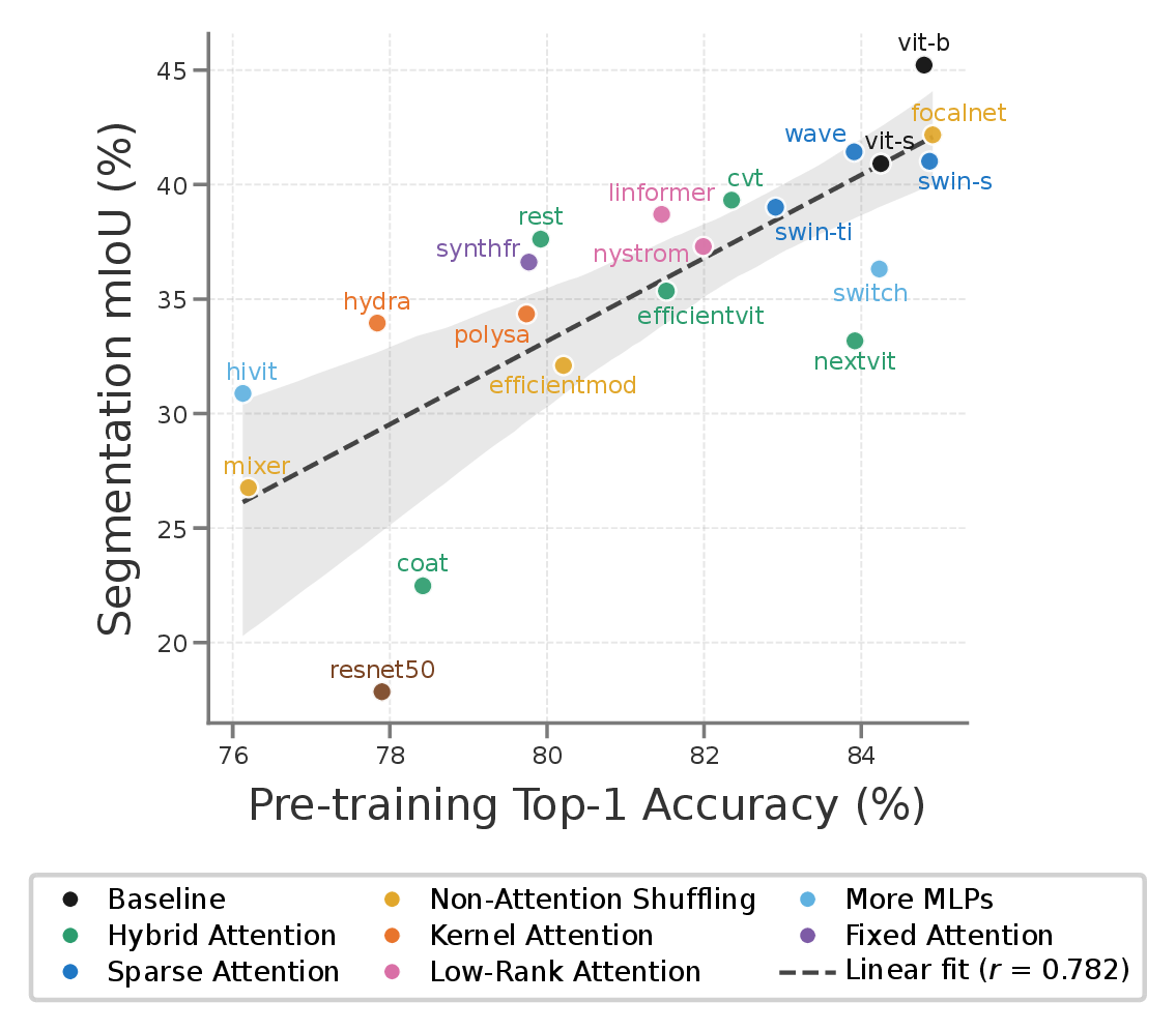
Now that we have established LUMA as a fair comparison tool, we can utilize it to measure segmentation efficiency across backbones. As visualized in 2, at the \(224\) px pre-training resolution, most mixers transfer to dense prediction without difficulty (plain ViT [8], WaveViT [32], Linformer [9], ResT [15], and Hydra [34] all reach mIoU values above the trend line) while a distinct set does not: ResNet-50 [43], CoaT [35], and NextViT [17], which all utilize convolutions, as well as Switch [37] are confined below the mean-transfer curve, contrasting BoB [20], who found supervised CNNs to be the best backbones. Note that ResT is the exception to this rule and that ResNet-50 and CoaT generalize better on Cityscapes (see 10). ViT, FocalNet [36], and WaveViT generalize well from classification to segmentation on ADE20K and Cityscapes. Across backbones, ImageNet top-1 accuracy is a moderate predictor of segmentation mIoU with Pearson \(r \approx 0.78\) for ADE20K at \(512\) px and \(r \approx 0.71\) for Cityscapes at \(1024\) px, but with significant outliers to the top and bottom.
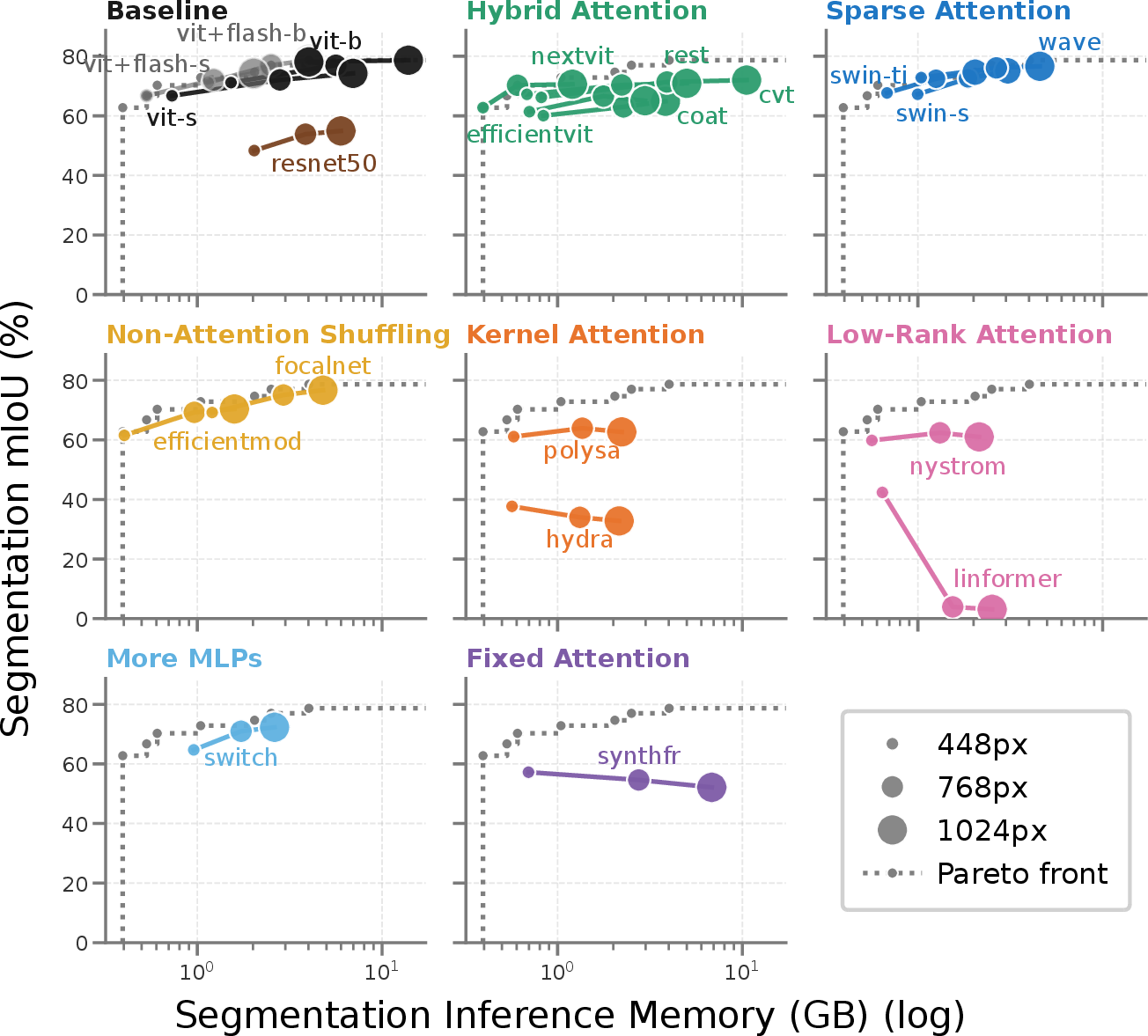
Transferring at \(224\) px does not imply transferring at the resolutions segmentation actually demands. Kernel, Low-Rank, and Fixed attention all have problems generalizing to higher resolutions: In 31, Linformer drops from \(38.4\) to \(3.8\) mIoU, Hydra from \(33.1\) to \(6.5\), and Synthesizer [24] from \(35.1\) to \(27.0\), inverting the \(+5\)–\(6\) mIoU gain that ViT and other healthy backbones obtain. Nystrom [11] increases performance only up to intermediate resolution.
In the throughput–mIoU trade-off (3), even without FlashAttention [66], [67], plain ViT still holds the Pareto frontier; the non-ViT models that reach it are sparse attention models (Swin-S [12] and WaveViT [32]), and FocalNet on Cityscapes. Enabling FlashAttention roughly doubles ViT’s throughput, displacing other models from the throughput–frontier. This exposes an implementation confound rather than a settled architectural verdict: Efficient mixers are measured with unoptimized kernels, and a comparably engineered implementation (e.g.a fused WaveViT) is the natural route to an efficient backbone that can better rival a hardware-optimized ViT with FlashAttention, as indicated by results relative to ViT without FlashAttention. When it comes to memory efficiency (see 4), the overall trend is similar: ViT is Pareto-optimal at the larger sizes with sparse attention (WaveViT and Swin-S) and non-attention shuffling (FocalNet [36] and EfficientMod [10]) closeby. At small memory footprints, hyrid models at small image resolutions cluster close to the Pareto–front.
A ViT backbone with FlashAttention is a solid choice (generalization and speed), with sparse attention models, or FocalNet as efficient alternatives.
Note however, that differences are generally small for the best ViT, hybrid, sparse, and non-attention models.
4.3 Which pretraining to use?↩︎
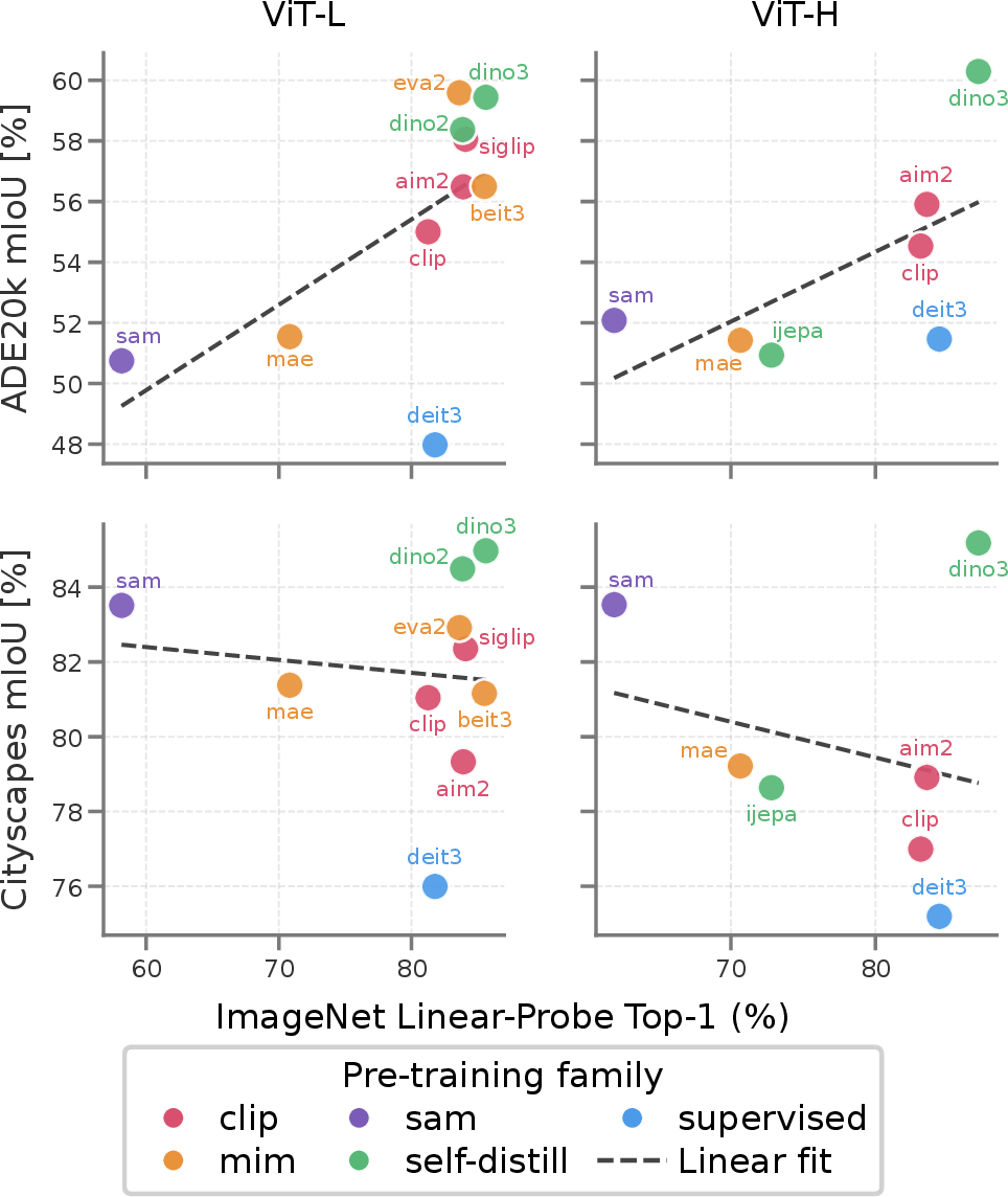
With the architecture fixed, the next question is which pretraining to initialize it with. The natural instinct is to pick the checkpoint based on the ImageNet linear-probe accuracy, since most papers publish it. 5 plots mIoU against ImageNet accuracy across 11 pretraining schemes under our unified recipe. A positive trend exists only on ADE20K but is weak and carried almost entirely by the extremes, as removing plain MAE [50], SAM [13], and supervised DeiT III [46] collapses the rank correlation among the remaining strong models to \(\rho = 0.21\) for ViT-L on ADE20K. On Cityscapes, the trend is even negative. The dominant signal is instead the pretraining objective. Dense objectives (masked image modeling, especially EVA-02 [52], and DINO’s [54], [55] self-distillation) meet or exceed the trend regardless of where they fall on ImageNet linear-probe, with EVA-02 the strongest model overall for ViT-L on ADE20K (59.7 mIoU) despite only mid-pack classification accuracy. On Cityscapes, DINOv3 is the best pretraining, closely followed by DINOv2 (for ViT-L). Interestingly, SAM’s [13] segmentation pretraining does not generalize to our setup on ADE20K, but performs very well (only DINO is better) on Cityscapes. Since supervised and clip pretraining decouples global, linearly-separable semantics from the per-patch spatial structure, it does not generalize well to dense tasks: DeiT III’s linear-probe (81.8% on mean patch-embedding) exceeds both CLIP [47] and plain MAE, yet its mIoU sits \(\approx 8\) p.p. below the trend prediction, while every other model lies within \(\pm 3.5\). CLIP itself also sits below the trend. We conclude that self-supervised approaches have improved a lot since BoB [20], when supervised pretraining was found best. Our practical recommendation is:
Initialize from a dense-objective foundation model (DINOv3 or EVA-02 work best) and disregard ImageNet linear-probe accuracy as a proxy.
Note, that 4.2 holds pretraining fixed to a shared supervised pretraining, a controlled test of transfer from identical conditions, since dense-objective pretrained states are not (yet) available for most architectures, besides ViT.
4.4 Compute-Optimal Scaling↩︎
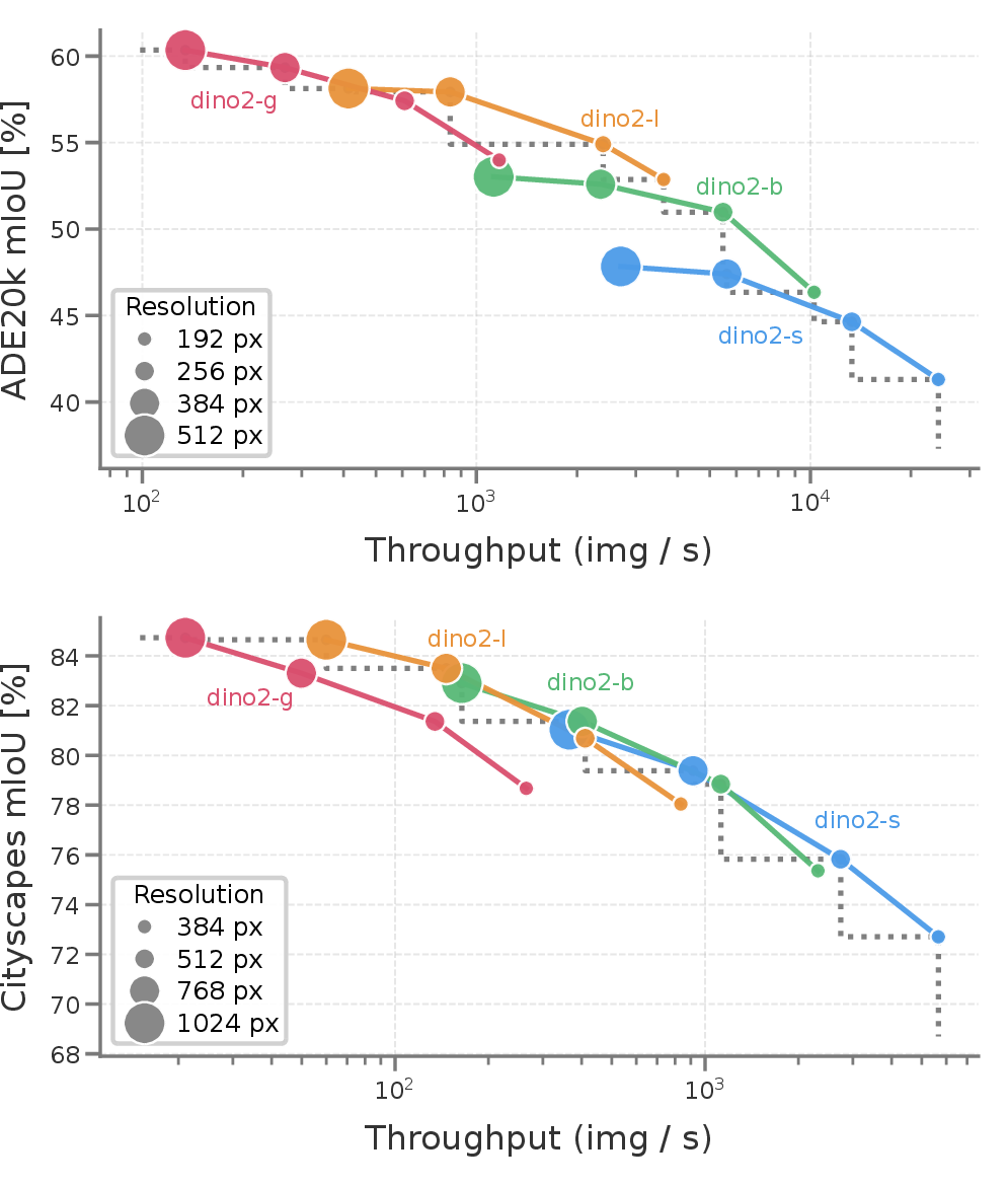
A fixed compute budget can be spent on a larger backbone or on higher input resolution. Both raise mIoU, but which is more efficient? We characterize the optimal trade-off by comparing DINOv2 [54] across backbone sizes and input resolutions under our unified recipe (see 6), we find that the Pareto–optimal models are identical whether cost is measured in FLOPs, inference memory, or latency, indicating a general allocation rule. Accuracy surfaces are well described by a saturating power law, mirroring the functional form used to model joint parameter–data scaling in language models [68] and compute scaling in vision [69]: \[\mathrm{mIoU}(N, R) \;=\; U - A\,N^{-\alpha} - B\,R^{-\beta}, \label{eq:surface}\tag{2}\] with parameter count \(N\) and resolution \(R\), fitting to within \(0.3\) mIoU on Cityscapes and \(0.7\) on ADE20K. Since inference cost follows \(C \propto N^{p} R^{q}\) with \(p=0.96\), \(q=2.21\) (\(R^2=0.999\)), minimizing 2 under a budget \(C\) yields closed-form compute-optimal trajectories \(N^\star \propto C^{e_N}\) and \(R^\star \propto C^{e_R}\) (derivation in 6).
The allocation is strongly asymmetric: we obtain \(e_N = 0.83\) on ADE20K and Cityscapes against \(e_R = 0.09\) and \(e_R = 0.10\), respectively. In practical terms, scaling the model alone at fixed resolution turns a \(10\times\) budget into two ViT size steps (S\(\to\)L); the optimal path instead diverts \(20\)–\(25\)% of the additional compute to resolution while buying a \(\approx 5\)–\(7\times\) larger backbone.
Two deviations from the fitted surfaces are themselves informative. First, on Cityscapes ViT-g is not compute-optimal: ViT-B at 1024 px outperforms it at 384 px by \(4.2\) mIoU using fewer FLOPs, and ViT-L at 1024 px beats it at 768 px by \(1.3\) mIoU at \(30\%\) less compute; the frontier is traced by S\(\to\)B\(\to\)L with resolution scaled alongside. On the harder ADE20K dataset, by contrast, ViT-g tops the frontier. Second, the resolution lever is bounded by native image resolution, which the largest sweep setting reaches on both datasets. All in all, the optimal scaling is:
Roughly \(80\%\) of additional compute should be spent on model size: \(N^\star \propto C^{0.83}\), with optimal token count growing only as \(T^\star \propto C^{0.2}\).
5 Conclusion↩︎
We ask which backbone is most efficient for segmentation and whether it’s ViT. Answering it required an instrument the literature lacks: a single lightweight head that attaches unchanged to any token mixer, so that a measured difference reflects the backbone and not the apparatus around it. LUMA is that instrument, and it carries a result complementary to EoMT’s [7]: Queries need not live inside the backbone’s attention at all; a minimal external read matches it.
Holding LUMA fixed across 20 backbones, 11 pretraining schemes, and a range of resolutions separates, for the first time under one modern recipe, what governs segmentation quality. Along the architecture axis the differences largely collapse: Good backbones from each family transfer within a narrow band, and novel token-mixer designs deliver neither the accuracy nor the efficiency they promise on the dense task, even with high-resolution inputs. The plain ViT holds the throughput–front, with efficient variants competitive only in memory. A few sequence-length-bound mixers collapse outright as resolution grows. Along the pretraining axis the task is decisive: Dense objectives transfer robustly, while supervised and multimodal contrastive pretraining fall systematically below the trend regardless of classification accuracy. Progress in self-supervised pretraining since BoB [20] suggests opportunities for further gains here. Along the scale axis the compute-optimal frontier is dominated by model size, which should absorb roughly \(80\%\) of any added budget. Architecture, the lever the field has tuned hardest, moves dense performance least; the pretraining objective and plain capacity move it most.
The thread through all three is that the proxies ranking models at classification — top-1 accuracy, linear-probe separability — can mislead for segmentation, because they reward globally separable semantics over the per-patch spatial structure dense prediction demands. The practical synthesis is therefore simple: Keep a simple architecture, initialize from a dense-objective foundation model, and spend added compute on model size before resolution. All in all, effort is best directed not at new token mixers, but at pretraining objectives and scalable architectures measured fairly on the dense task itself, which LUMA now makes possible.
Acknowledgements↩︎
This work was funded by the Carl-Zeiss Foundation under the Sustainable Embedded AI project (P2021-02-009). All compute was done thanks to the Pegasus cluster at DFKI Kaiserslautern.
6 Compute-optimal allocation: derivation↩︎
We use the \(4{\times}4\) size–resolution sweep of Section 4.4 to fit our scaling-laws: ViT-{S, B, L, g} with DINOv2 [54] pretraining, trained with LUMA at \(\{384, 512, 768, 1024\}\) px on Cityscapes [23] and \(\{192, 256, 384, 512\}\) px on ADE20K [22]. All runs share the head configuration, patch size, optimizer, and schedule and each configuration is trained at its target resolution. mIoU is always computed at full ground-truth resolution, so accuracies are comparable across input resolutions.
We fit \(\log C = \log k + p \log N + q \log R\) on measured inference FLOPs across all configurations, obtaining \(p = 0.96\), \(q = 2.21\) with \(R^2 = 0.999\). We fit the mIoU scaling law (Equation (2)) per dataset by nonlinear least squares (multi-start, \(U\) bounded above by 100). The two error terms are additive and separable, which the data supports: residuals show no \(N \times R\) interaction structure beyond the two deviations discussed below. 2 reports all fits. Because ViT-g falls below the accuracy of ViT-L on Cityscapes, we report the S/B/L fit as primary there; on ADE20K, excluding ViT-g drives the fitted ceiling \(U\) to its bound and is reported only as a sensitivity.
| Dataset | Sizes | \(n\) | \(\alpha\) | \(\beta\) | RMSE | \(e_N\) | \(e_R\) |
|---|---|---|---|---|---|---|---|
| Cityscapes | S/B/L | 11 | 0.13\(^\dagger\) | 1.11 | 0.30 | 0.83 [0.66, 0.88] | 0.10 [0.08, 0.15] |
| Cityscapes | S/B/L/g | 14 | 0.35 | 0.84 | 0.41 | 0.50 [0.34, 0.66] | 0.21 [0.15, 0.26] |
| ADE20K | S/B/L/g | 16 | 0.29 | 2.77 | 0.71 | 0.83 [0.74, 0.87] | 0.09 [0.07, 0.13] |
| ADE20K | S/B/L | 12 | 0.09\(^\dagger\) | 3.00 | 0.46 | 0.97 [0.96, 0.97] | 0.03 [0.03, 0.03] |
Minimizing \(E(N, R) = A N^{-\alpha} + B R^{-\beta}\) subject to \(k N^{p} R^{q} = C\), stationarity of the Lagrangian in log-coordinates gives \[\frac{\alpha A N^{-\alpha}}{p} \;=\; \frac{\beta B R^{-\beta}}{q}, \label{eq:stationarity}\tag{3}\] i.e.the marginal error reduction per unit of log-compute is equalized across the two levers. 3 implies \(N^{-\alpha} \propto R^{-\beta}\) along the optimal path; differentiating this relation together with the constraint \(p\,\mathrm{d}\!\log N + q\,\mathrm{d}\!\log R = \mathrm{d}\!\log C\) yields \[e_N = \frac{\beta}{p\beta + q\alpha}, \qquad e_R = \frac{\alpha}{p\beta + q\alpha}, \qquad E^\star \propto C^{-\frac{\alpha\beta}{p\beta + q\alpha}}, \label{eq:exponents}\tag{4}\] which satisfy \(p\,e_N + q\,e_R = 1\) by construction. Numerically, the optimal error decays as \(E^\star \propto C^{-0.11}\) on Cityscapes and \(C^{-0.25}\) on ADE20K. Confidence intervals in 2 are obtained by refitting on 300 bootstrap resamples of the runs and propagating through 4 .
Two limitations bound these estimates:
Both sweeps reach native image resolution at their largest setting, so \(R^\star\) extrapolations beyond it are meaningless; within the sweep.
Excluding ViT-g (on Cityscapes only, where it falls below ViT-L) restricts that fits parameter span to \(13\times\) across three sizes, which widens the \(e_N\) interval and creates the \(U\)–\(\alpha\) degeneracy noted in 2; on ADE20K all sizes are retained.
7 Hyperparameters & Setup↩︎
We describe our setup for training and evaluation using LUMA.
7.1 Training Setup.↩︎
Every backbone in the benchmark is trained with the identical recipe below; the only quantities that vary per backbone are the pretrained checkpoint, the patch size, and the per-depth LLRD assignment (which depends on block count). No per-backbone hyperparameter tuning is performed, so that any difference in mIoU is attributable to the architecture rather than to optimization.
We optimize with AdamW at a base learning rate of \(1{\times}10^{-4}\) and weight decay \(0.05\), in bf16-mixed precision. LLRD [70] with factor \(0.8\) is applied across the backbone, the pretrained non-block parameters (patch and positional embeddings) take the maximum discount \(\text{lr}\times 0.8^{\,N-1}\), and the LUMA queries, heads, and upscale modules train at the full base rate. The backbone is fine-tuned, not frozen: a two-stage warmup holds it at zero learning rate for the first \(500\) steps while the new LUMA modules warm up linearly over the same window, after which the backbone ramps linearly over \(1000\) steps; both groups then follow cosine decay to zero. We use
\(100\) learnable queries and inject interleaved cross-attention into the last \(L_2=2\) encoder blocks for every backbone.
We adopt the Hungarian-matched Mask2Former loss [2]: cross-entropy on the class logits (weight \(2.0\), with \(\varnothing\)-class weight \(0.1\)), and binary cross-entropy (weight \(5.0\)) plus Dice loss (weight \(5.0\)) on the mask logits. The mask loss is computed on \(12544\) points sampled with oversample ratio \(3.0\) and importance-sample ratio \(0.75\).
Augmentation is identical on both datasets: random horizontal flip, scale jitter in \((0.5, 2.0)\), random crop to the training resolution, and color jitter (brightness \(\pm 32/255\), contrast and saturation \(\pm 0.5\), hue \(\pm 18^\circ\)).
| Setting | ADE20K | Cityscapes |
|---|---|---|
| Train resolution | \(512\times512\) | \(1024\times1024\) |
| Classes | \(150\) | \(19\) |
| Batch size / GPU | \(8\) | \(4\) |
| GPUs | \(2\) | \(4\) |
| Effective batch size | \(16\) | \(16\) |
| Epochs | \(32\) | \(108\) |
The two datasets differ only in the quantities listed in 3. At validation both use sliding-window inference: the image is resized so its short side matches the training resolution, tiled with overlap, and the window logits are averaged.
7.2 Efficiency Evaluation.↩︎
All efficiency numbers are measured on a single NVIDIA H100 in bf16 with torch.compile enabled (it is disabled during training). FLOPs are computed with fvcore 2. In Section 4.1 where LUMA is compared against external baselines, FLOPs and FPS account for the full sliding-window inference and FPS is reported at single-image (batch size \(1\))
latency, matching the comparison protocol of EoMT [7]. The remaining sections report inference throughput at the optimal batch size and do not fold
in the windowing factor, since that factor is constant across all LUMA variants and cancels in any cross-backbone comparison.
| Backbone | Pretraining | ADE20K | Cityscapes | |||
|---|---|---|---|---|---|---|
| 3-4 (lr)5-6 | mIoU (%) | Std (%) | mIoU (%) | Std (%) | ||
| ViT-L | DINOv2 | 58.44 | 0.38 | 84.65 | 0.01 | |
| ViT-B | DeiT III | 50.42 | 0.27 | 78.64 | 0.04 | |
| FocalNet-S-Srf | DeiT III | 48.07 | 0.18 | 76.58 | 0.15 | |
| WaveViT-S | DeiT III | 47.13 | 0.63 | 76.46 | 0.24 | |
8 Run-to-Run Variance↩︎
Since it is infeasible to run every one of our benchmark experiments multiple times, we verify run-to-run variance on a representative subset of configurations. We re-train these configurations two additional times (\(N=3\)) with only the random seed varying, to make sure that the single-run results of the main benchmark are significant. 4 reports the resulting spread on ADE20K and Cityscapes. The mean standard deviation on ADE20K is \(0.37\) mIoU, with even lower \(0.11\) mIoU on Cityscapes. Treating the floor as homoscedastic, two single runs are expected to differ by more than \(1.1\) mIoU in only \(\sim\) 5% of cases on ADE20K. All comparisons on which our conclusions rest span several mIoU and therefore exceed this run-to-run noise by a wide enough margin, confirming that single-seed reporting is sufficient for the analysis.
9 Ablating LUMA↩︎
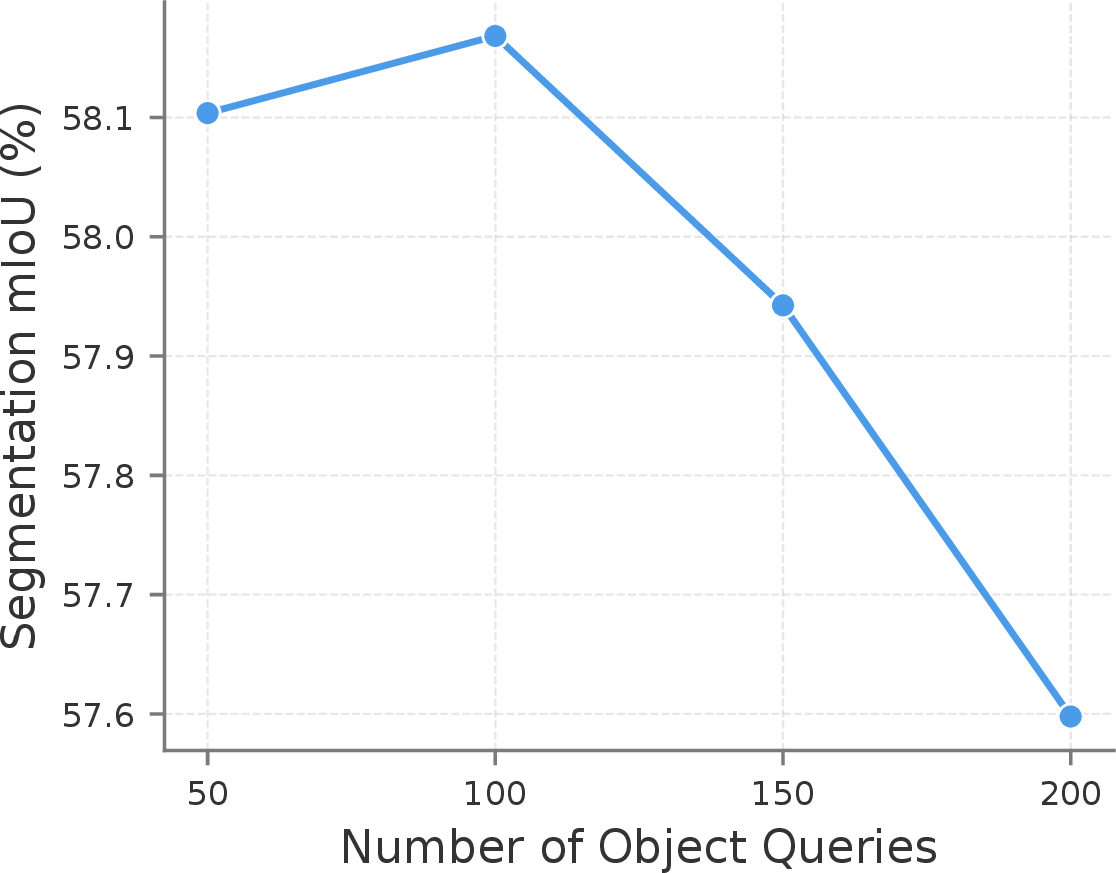
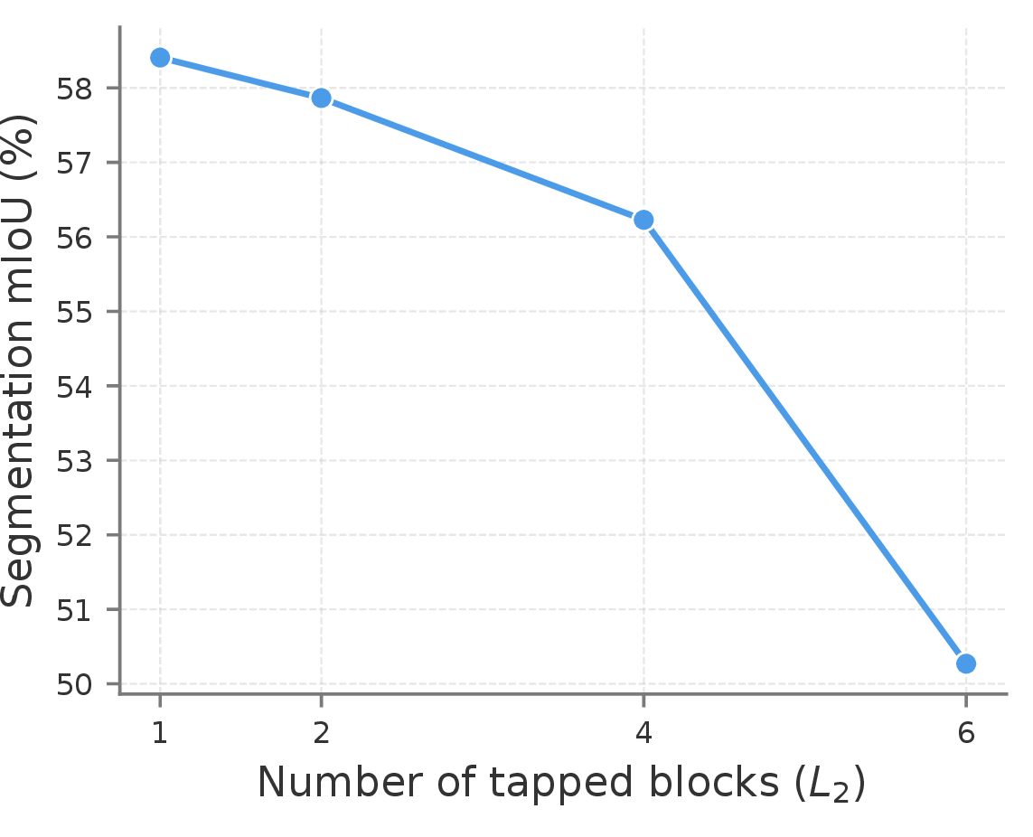
Figure 7: LUMA Ablations (ADE20K). Left: Number of queries. We keep EoMT’s default of \(100\) queries. Right: Number of tapped blocks. Interestingly, more tapped backbone blocks reduce performance and a single token read works best..
7 ablates the number of queries and cross-attention reads \(L_2\) on ADE20K. The left panel confirms EoMT’s default of \(100\) queries is also optimal for LUMA, though the effect is small: mIoU stays within \(57.6\)–\(58.2\) across \(50\)–\(200\) queries. Additionally, making the queries not pass through the backbone’s MLP blocks slightly reduces performance from \(58.2\) to \(58.1\) mIoU. Surprisingly, the right panel shows a monotonic downward trend of mIoU as \(L_2\) grows, from \(58.4\) at \(L_2 = 1\) to \(50.3\) at \(L_2 = 6\). Thus, a single cross-attention read of the patch tokens is enough to recover EoMT’s performance.
10 More Benchmark Plots↩︎
10.1 Backbones↩︎
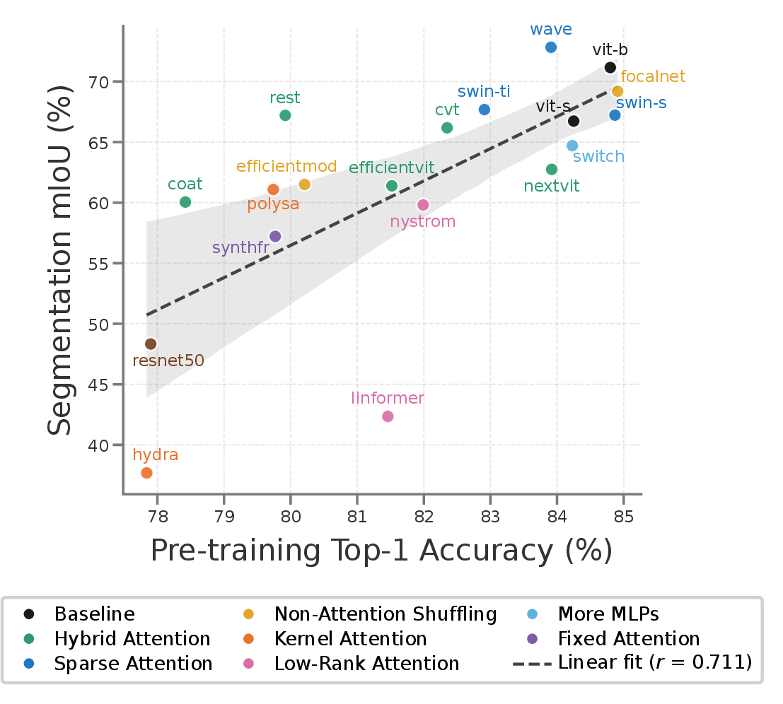
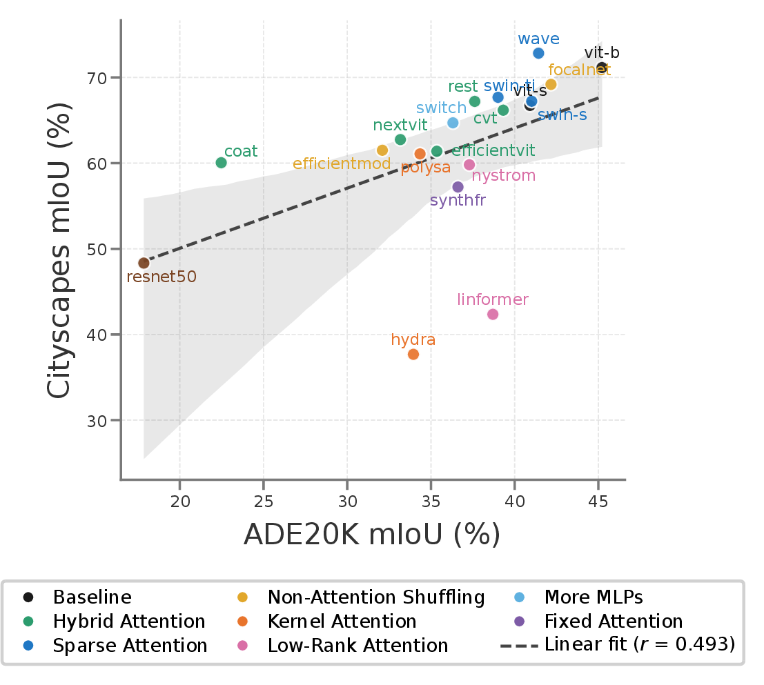
Figure 8: Comparison of backbone quality across different tasks. (a) ImageNet top-1 vs.Cityscapes mIoU. (b) ADE20K mIoU vs.Cityscapes mIoU. Hydra and linformer perform comparatively bad on Cityscapes, because their resolution-scaling issues.. a — Pretraining accuracy vs Cityscapes mIoU., b — ADE20K mIoU vs Cityscapes mIoU.
8 extends cross-task correlation analysis to Cityscapes. ImageNet-1k top-1 tracks Cityscapes mIoU about as loosely as it tracks ADE20K mIoU (\(r=0.71\)), so linear-probe accuracy is a weak segmentation proxy on both datasets. The cross-task panel is more telling: the two segmentation benchmarks agree with each other (\(r=0.49\)) less than either agrees with classification, despite measuring the same task. The deviation is concentrated rather than diffuse—LUMAlinformer and LUMAhydra lie on the ADE20K trend at \(512\,\mathrm{px}\) but collapse on Cityscapes, whose higher inference resolution drives the token count past the regime their sequence-length-bound mixing was calibrated for. These failures are resolution-dependent, not capacity-dependent, and confirm that no single benchmark exposes how an architecture scales across the resolutions segmentation actually spans.
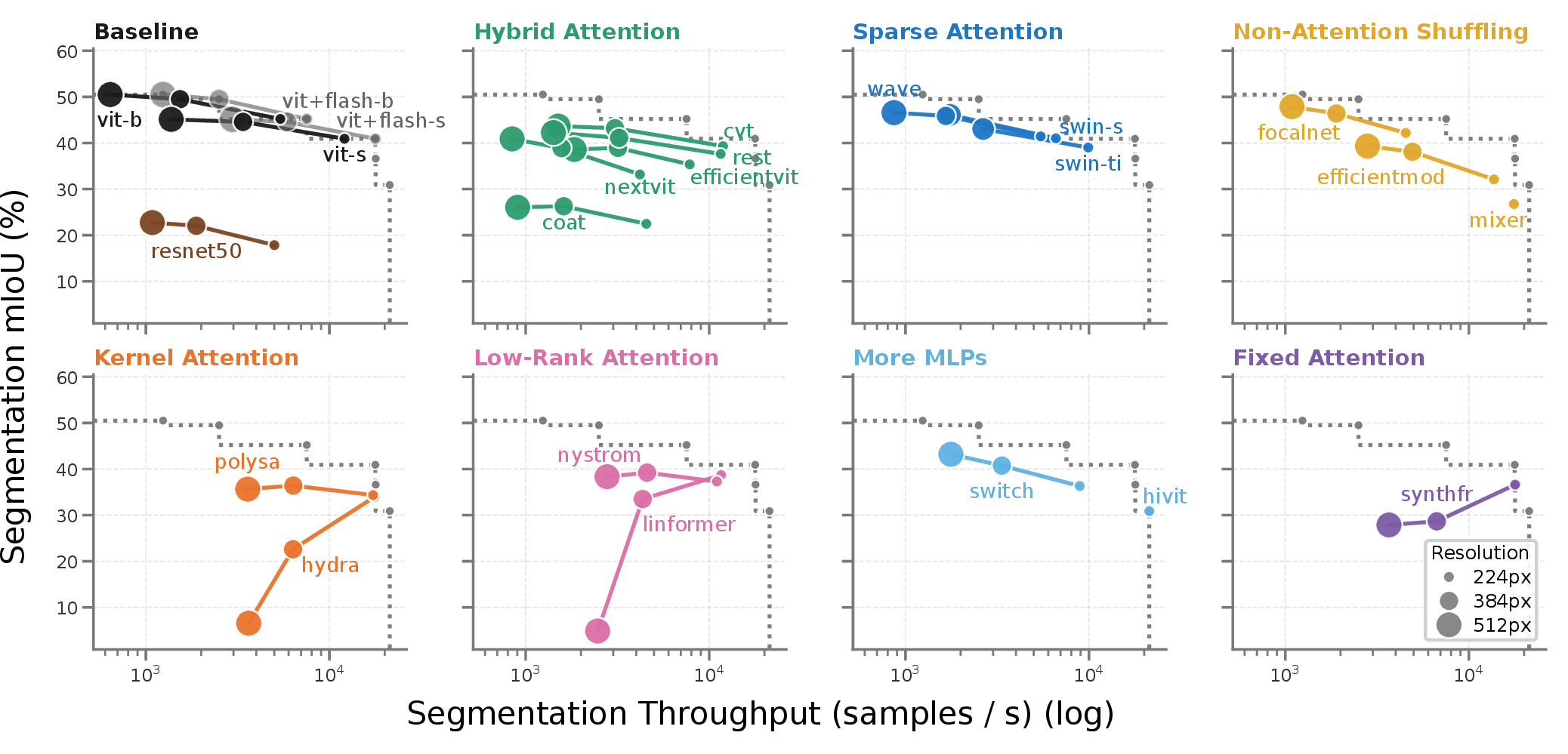
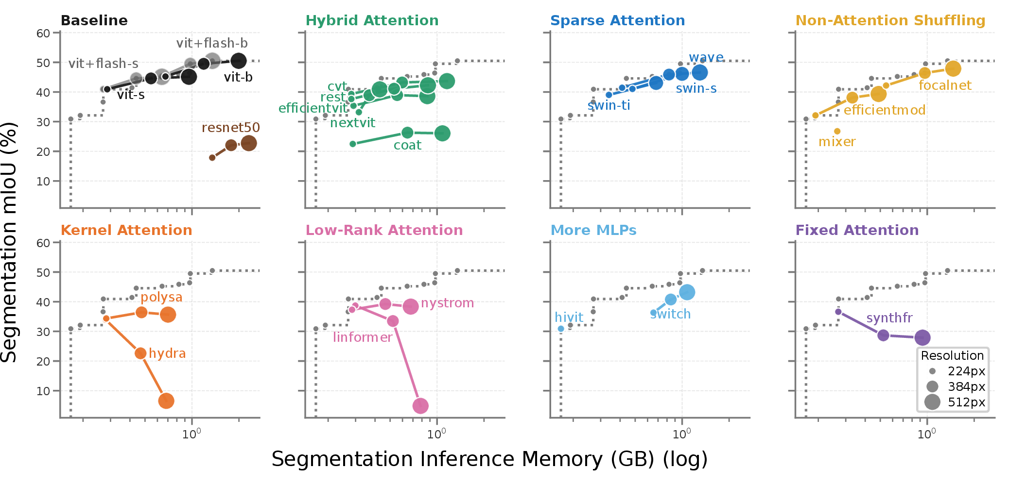
Figure 9: Efficiency on ADE20K. Segmentation throughput (a) and inference memory (b) versus mIoU, with families grouped as in [31] and marker size encoding image resolution; the dotted line marks the Pareto front. ViT+FlashAttention holds both frontiers; among efficient backbones only sparse attention (Swin-S, Wave) and non-attention shuffling (FocalNet, EfficientMod) approach it. Kernel, low-rank, and fixed mixers leave the frontier as resolution rises.. a — Throughput vs ADE20K mIoU., b — Inference memory vs ADE20K mIoU.
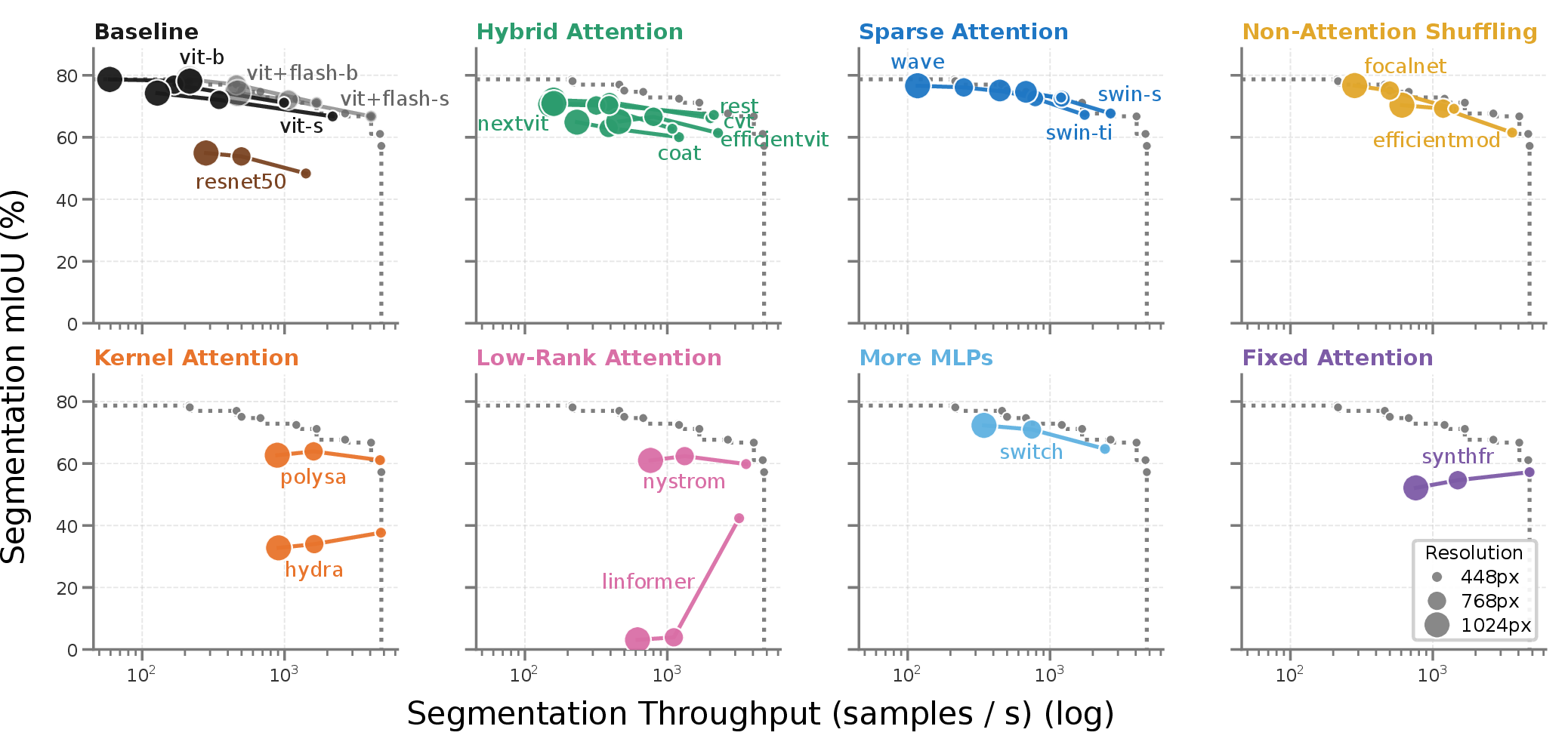
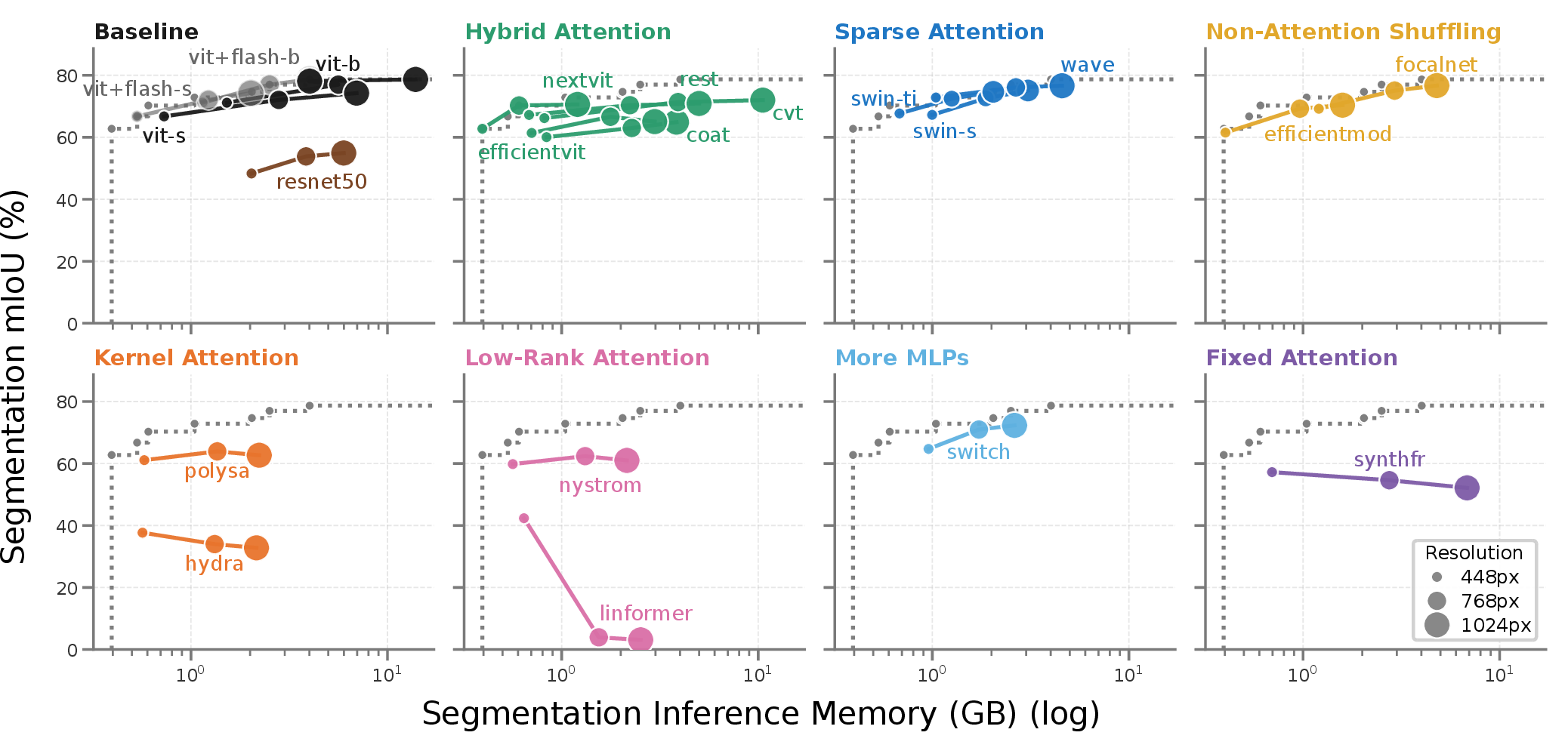
Figure 10: Efficiency on Cityscapes. Segmentation throughput (a) and inference memory (b) versus mIoU; conventions as in 9. The ADE20K ordering carries over, and the collapse of the sequence-length-bound mixers is more severe at Cityscapes’ higher inference resolutions of up to \(1024\) px.. a — Throughput vs Cityscapes mIoU., b — Inference memory vs Cityscapes mIoU.
[fig:eff-ade,fig:eff-city] complete the efficiency grid, plotting both throughput and inference memory against mIoU on both datasets. The throughput–ADE20K panel (9a) and the memory–Cityscapes panel (10b) restate Figures 3 and 4 of the main paper; the remaining two panels are new and corroborate the verdict. The frontier is held by ViT+FlashAttention on every axis and dataset, with sparse attention (Swin-S, Wave) closest and FocalNet and EfficientMod close on the memory axis. The same kernel, low-rank, and fixed mixers leave both frontiers as resolution grows. Cityscapes makes this sharper: its inference resolutions (\(448\)–\(1024\) px) exceed ADE20K’s (\(224\)–\(512\) px), pushing the largest markers further into the sequence-length regime these mixers cannot cover.
10.2 Compute Scaling↩︎
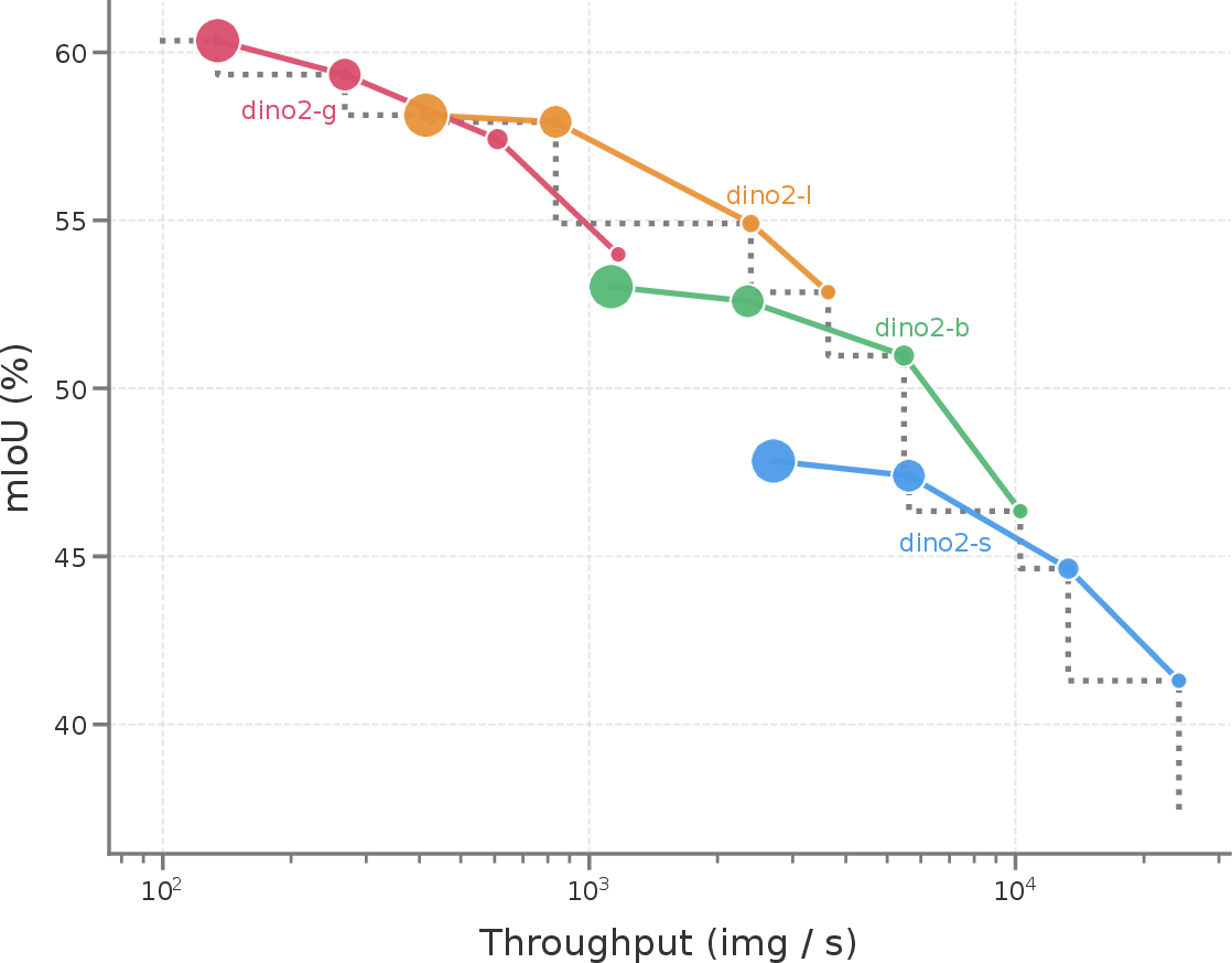
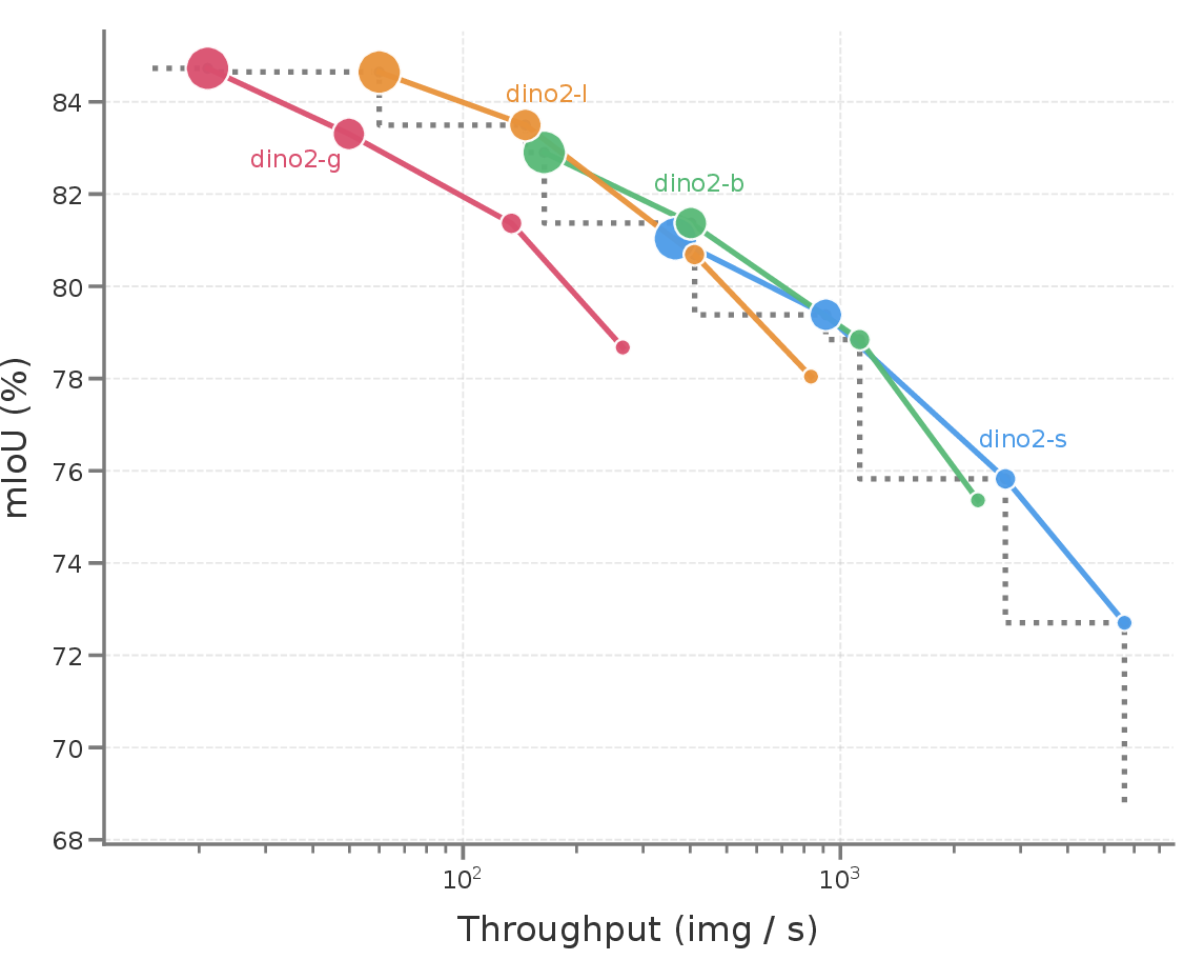
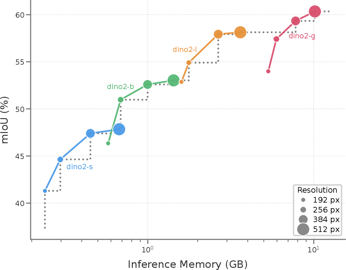
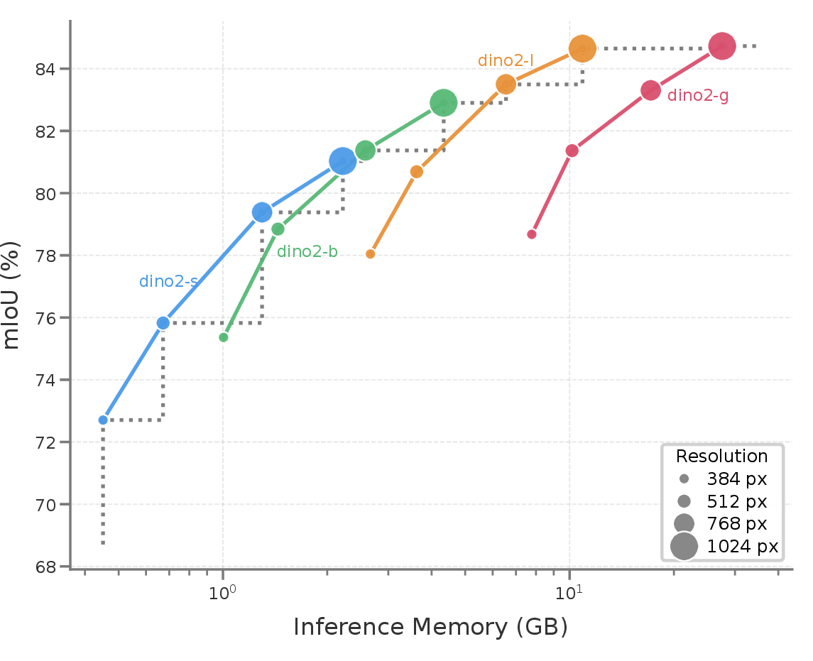
Figure 11: Compute-optimal scaling on both efficiency axes. The DINOv2 sweep (DINOv2-S/B/L/g across resolutions) plotted against throughput (a, b) and inference memory (c, d), on ADE20K (a, c) and Cityscapes (b, d); marker size encodes resolution and the dotted line marks the Pareto front. On every axis and dataset the front is climbed by model size, with resolution contributing the finer steps; the compute-optimal fit (6) directs roughly \(80\%\) of added compute to model size.. a — Throughput vs ADE20K mIoU., b — Throughput vs Cityscapes mIoU., c — Inference memory vs ADE20K mIoU., d — Inference memory vs Cityscapes mIoU.
11 extends Figure 6 of the main paper to all four efficiency–accuracy combinations, adding the inference-memory axis to the throughput axis of the main paper. Panels (a) and (b) restate Figure 6 of the main paper; panels (c) and (d) plot the same DINOv2 sweep against inference memory and are new. On every panel the Pareto front is climbed by model size, with the DINOv2-S/B/L/g progression tracing the frontier and the resolution increments within each model contributing the smaller steps. The memory panels address a confound: the compute-optimal conclusion of Figure 6 from the main paper is a FLOPs argument, and a memory-bound reading could in principle favour the lower-resolution, smaller-activation regime, but the front is climbed by the same progression on the memory axis, so the verdict does not depend on which efficiency budget is charged. The cross-dataset asymmetry also carries over: on ADE20K resolution saturates near the native image size, leaving model size as the only remaining lever and placing DINOv2-g at the top of the frontier, whereas on Cityscapes the higher native resolution still rewards resolution scaling, and DINOv2-g is not compute-optimal at intermediate budgets and a smaller model at higher resolution dominates it (DINOv2-B at \(1024\) px beats DINOv2-g at \(384\) px at fewer FLOPs).