Goal-Oriented Space-Time Adaptivity for the Navier–Stokes Equations based on the Dual Weighted Residual Method
July 01, 2026
Abstract
This work presents a goal-oriented a posteriori error estimator based on the Dual Weighted Residual (DWR) method together with space-time mesh adaptivity for the Navier–Stokes equations. The resulting nonlinear algebraic systems on the space-time slabs are solved by Newton’s method with GMRES, preconditioned by a slab-wise geometric multigrid method. This combination yields reliable control of target quantities on computationally feasible space-time meshes together with a robust and efficient solution of the algebraic systems. The implementation is based on a MPI-parallel programming model in the deal.II library. Further ingredients are a discontinuous Galerkin discretization in time and inf-sup stable finite element pairs with discontinuous pressure on tensor-product meshes. The performance of the approach is investigated in benchmark computations with regard to accuracy, efficiency, and stability.
Keywords: Navier–Stokes Equations \(\cdot\) Goal-Oriented Error Control \(\cdot\) Dual Weighted Residual Method \(\cdot\) Space-Time Adaptivity \(\cdot\) Geometric Multigrid Method \(\cdot\) Local Vanka Smoother \(\cdot\) Nitsche Method
1 Introduction↩︎
The accurate numerical simulation of incompressible viscous fluid flow governed by the Navier–Stokes equations remains challenging, in particular when strong dynamics and fine-scale structures in space and time have to be resolved. The robust and efficient solution of the arising algebraic systems adds a further layer of complexity. Moreover, algorithms that address these challenges have to be implemented in a software framework that is suitable for computations on modern hardware architectures with tens of thousands of compute cores, including hybrid CPU and GPU systems. This places high demands on the underlying data structures. In this work, we design an approach that addresses these requirements. The implementation is based on the deal.II library [1].
Space-time mesh adaptation based on rigorous error representations, or on indicators derived from such representations, has been shown to yield accurate results on computationally feasible grids at moderate numerical cost, even for problems with complex solution structures [2], [3]. Among these approaches, the Dual Weighted Residual method (DWR) [4] offers the possibility of controlling the discretization error in user-defined goal quantities of practical interest. The key idea of this approach is to compute dual weights for the local residuals entering the error representation. This requires the solution of the generally nonlinear primal problem and its linearized dual problem by space-time finite element methods. The DWR method has been successfully applied to numerous problem classes, including fluid flow [5], [6], wave propagation [7], fluid-structure interaction [8], [9], among others. For a comprehensive review with detailed references on various model problems, we refer, for instance, to [4], [8], [10]. Error control in norms associated with the weak formulation constitutes a conceptually different class of techniques for a posteriori error estimation and automatic mesh adaptation. For this, an approach using equilibrated flux reconstructions is proposed in [11].
The DWR concept relies on solving the primal Navier–Stokes system and the associated linearized dual problem by space-time finite element methods. Both, lower- and higher-order approximations, in space and time are of interest. They should maintain stability and preserve as much of the structure of the continuous problem as possible. For the time discretization we use the discontinuous Galerkin method [12], [13]. In space, we employ inf-sup stable finite element pairs with discontinuous pressure. Discontinuous pressure approximations have demonstrated advantages over continuous ones [14]. Moreover, they are advantageous for the construction and application of the slab-wise local Vanka smoother within the geometric multigrid preconditioner. Nonhomogeneous Dirichlet boundary conditions are imposed by Nitsche’s method [15], which leads to a strictly variational formulation rather than enforcing the boundary data through the definition of the function spaces and algebraic systems.
We localize the space-time finite element approximation of the primal and dual DWR problems to space-time slabs \(\Omega\times (t_{n-1},t_n]\), where \(\Omega \subset \mathbb{R}^d\) with \(d \in \{2,3\}\). This yields a time-marching approach. For higher polynomial degrees in time and high spatial resolution, the arising algebraic systems already become large, and the Newton-linearized Jacobian has a complex block structure that complicates the construction of efficient preconditioners. Holistic space-time finite element frameworks, in which all time steps are solved fully coupled and simultaneously, have also been studied yet; cf., e.g., [16]–[19]. Their feasibility continues to remain an open problem if three space variables and a huge number of time steps are involved. The lack of efficient preconditioning techniques for such systems still limits the application of holistic approaches. For this reason, we use a slab-wise approach with a tensor-product mesh structure in this work.
For the slab-wise solution of the Newton-linearized primal problems and of the linear dual problems, we apply a Flexible Generalized Minimum RESidual (FGMRES) method preconditioned by a single \(V\)-cycle of a geometric multigrid (GMG) method. Nowadays, multigrid techniques are typically used as preconditioners for Krylov subspace methods rather than as stand-alone solvers. GMG methods have been studied extensively for the iterative solution of discrete systems arising from stationary partial differential equations. For this we refer to the pioneering work [20]. Owing to their optimal linear complexity, GMG methods are highly efficient and robust for this class of problems [21]. They have also been generalized in several directions, including \(hp\) multigrid methods based on hierarchies of polynomial degrees and meshes. For space-time finite element approximations of the Navier–Stokes equations, block systems with generalized saddle-point structure arise, where the precise block structure depends on the ordering of the slab unknowns [22], [23]. For such systems, the smoothing procedure is decisive for the overall efficiency of the multigrid preconditioner. In the present work, we use a local Vanka smoother, which can be interpreted as a non-overlapping Schwarz method. It is among the most effective smoothers for saddle-point problems, although its cost increases with the polynomial degree and with the number of space-time unknowns [23]. Algebraic MultiGrid (AMG) methods, a further class of multigrid techniques, perform damping of high frequency errors in the solution to linear systems and coarse grid corrections on the algebraic level and do not need any geometric information for building a hierarchy of problems [24], [25]. However, memory usage limits the application of AMG if large scale systems are encountered.
In this work, we study the combination of DWR error estimation, automatic space-time mesh adaptation, and slab-wise geometric multigrid preconditioning for the Navier–Stokes equations. The focus is on goal-oriented adaptivity and its interaction with a GMG-preconditioned Newton–Krylov method. For this purpose, we combine a DWR a posteriori error estimator with adaptive space-time refinement and GMRES iterations preconditioned by slab-wise geometric multigrid. The implementation uses MPI parallelization in deal.II, discontinuous Galerkin time discretization, and inf-sup stable finite element pairs with discontinuous pressure on tensor-product meshes. On benchmark computations, we assess estimator quality, reduction of the goal error relative to total computational work, and solver performance for both primal and adjoint problems. A central question we address is whether the gain from goal-oriented adaptivity justifies the additional cost of the adjoint solve and how this trade-off interacts with the robustness of the solvers.
This work is organized as follows. In Sec. 2, we present the weak form as well as the space-time discretization schemes. In Sec. 3, we derive an a posteriori error representation for the model problem. In Sec. 4, we discuss practical aspects of the implementation as well as the underlying space-time adaptive algorithm. In Sec. 5, we present the results of our numerical examples. Finally, Sec. 6 summarizes the results and outlines directions for future research.
2 Model Problem and Discretization in Space and Time↩︎
In this work, we investigate the accurate and efficient numerical simulation of incompressible viscous flow modeled by the nonstationary Navier–Stokes equations In 1 , we denote by \(Q=\Omega \times I\) the space-time domain, where \(\Omega\subset \mathbb{R}^d\), with \(d=2\) or \(d=3\), is a polygonal or polyhedral bounded domain with Lipschitz boundary \(\partial\Omega\) and \(I=(0,T)\), with \(0 < T < \infty\), is a finite time interval. The flow behavior at the boundary \(\partial\Omega = \Gamma_{D} \cup \Gamma_{\textrm{outflow}}\) is modeled by a function \(\boldsymbol{v}_D\) on the segments \(\Gamma_D\coloneq\Gamma_{\textrm{inflow}} \cup \Gamma_{\textrm{wall}}\), that prescribes an inflow profile \(\boldsymbol{v}_{\textrm{in}}\) on \(\Gamma_{\textrm{inflow}}\) and a no-slip condition \(\boldsymbol{v}=\boldsymbol{0}\) on the fixed wall segment \(\Gamma_{\textrm{wall}}\), as well as a so-called “do-nothing” condition on the artificial boundary segment \(\Gamma_{\textrm{outflow}}\). For this refer to [26], [27]. The velocity field \(\boldsymbol{v}\) and the pressure variable \(p\) are the unknown variables. The parameter \(\nu>0\) denotes the fluid’s viscosity, \(\boldsymbol{f}\) is a given volume force density, and \(\boldsymbol{v}_{0}\) is the initial value.
For the sake of brevity, we present the continuous and semidiscrete in time variational problem for homogeneous Dirichlet boundary conditions only. The mixed boundary conditions in 1 are incorporated in the fully discrete system and derivation of the duality based a posteriori error estimation; cf. Remark 2. Further, they are used in one of our numerical experiments. Throughout, we use standard notation for Sobolev and Bochner spaces. In particular, by \(L_\sigma^2(\Omega)^d\) we denote the \(L^2\)-closure of the set of divergence-free test functions on \(\Omega\). For the existence, uniqueness and regularity of weak solutions to the Navier–Stokes equations such that all of the arguments and terms used below are well-defined, we refer to the literature, cf., e.g., [26], [28], [29].
2.1 Weak Form and Discretization in Space and Time↩︎
For the discretization in space and time we follow the lines of [5], [22]. The variational formulation of 1 reads as:
For \(\boldsymbol{f} \in L^2(I;H^{-1}(\Omega)^{d})\) and \(\boldsymbol{v}_{0}\in L_\sigma^2(\Omega)^d,\) find \(\boldsymbol{u}\coloneq\{\boldsymbol{v},p\}\in
X\) such that \[\label{eq:2:weakform}
A(\boldsymbol{u})(\boldsymbol{\varphi}) = F(\boldsymbol{\psi}) \quad \forall \boldsymbol{\varphi}\coloneq\{\boldsymbol{\psi},\xi\} \in X\,,\tag{2}\] where the semi-linear form \(A(\cdot)(\cdot)\) and the
linear form \(F(\cdot)\) are defined by \[\begin{align}
\tag{3}
A(\boldsymbol{u})(\boldsymbol{\varphi}) & \coloneq &
\int_{I}\big\{(\partial_t \boldsymbol{v},\boldsymbol{\psi})
+ a(\boldsymbol{u})(\boldsymbol{\varphi})
\big\} \mathrm{d} t\;
+ (\boldsymbol{v}(0),\boldsymbol{\psi}(0) )\,,
\\[1.5ex]
\tag{4}
F(\boldsymbol{\psi}) & \coloneq & \int_I(\boldsymbol{f},\boldsymbol{\psi})\;\mathrm{d}t + (\boldsymbol{v}_{0},\boldsymbol{\psi}(0) ) \,,
\end{align}\] with the inner semi-linear form \(a(\cdot)(\cdot)\) given by
\[\label{eq:5:inSLFa}
a(\boldsymbol{u})(\boldsymbol{\varphi}) \coloneq \nu(\nabla \boldsymbol{v}, \nabla \boldsymbol{\psi})
+(\boldsymbol{v}\cdot \nabla \boldsymbol{v}, \boldsymbol{\psi})
-(p,\nabla\cdot\boldsymbol{\psi})
+ (\nabla\cdot\boldsymbol{v},\xi)\,.\tag{5}\] Here, \((\cdot,\cdot)\) denotes the inner product on \(L^2(\Omega)\) (or \(L^2(\Omega)^d\)) and
the underlying function space \(X\) is defined as \[\label{eq:6:X}
X\coloneq\{\boldsymbol{u}=\{\boldsymbol{v},p\}, \boldsymbol{v}\in L^2\big(I;H_0^1(\Omega)^d\big),
\partial_t\boldsymbol{v}\in L^2\big(I;H^{-1}(\Omega)^d\big), p\in L^2\big(I;L_0^2(\Omega)\big)\}\,.\tag{6}\] For the semi-discretization in time we use a discontinuous Galerkin method dG(\(r\)) with an
arbitrary polynomial degree \(r\ge 0\). Let \(\mathcal{T}_{\tau}\,=\{0\}\cup I_1 \cup \cdots \cup I_N\) be a partition of the closure of the time domain \(\bar{I}=[0,T]\) with left-open subintervals \(I_n\coloneq(t_{n-1},t_n]\), \(n=1,\dots,N\), with \(0=:t_0<t_1<\dots<t_N\coloneq
T\) and time step sizes \(\tau_n=t_n-t_{n-1}\) and the global time discretization parameter \(\tau=\max_{n}\,\tau_{n}\). On the subintervals \(I_n\),
we define the time-discrete function space \(X_{\tau}^{r}\) as \[\label{eq:7:Def95X95tau95r}
\begin{align}
X_{\tau}^{r} \coloneq \Big\{ & \boldsymbol{u}_{\tau}=\{\boldsymbol{v}_{\tau},p_{\tau}\}\in L^{2}\big(I; H_0^1(\Omega)^d\times L_0^2(\Omega)\big)\big| \boldsymbol{v}_{\tau}|_{I_{n}}\in \mathcal{P}_{r}\big(I_{n}; H_0^1(\Omega)^d\big),\\ &
\boldsymbol{v}_{\tau}(0)\in L^2(\Omega)^d, p_{\tau} \in \mathcal{P}_{r}\big(I_{n}; L_0^2(\Omega)\big)\,, n=1,\dots,N
\Big\}\,,
\end{align}\tag{7}\] where \(\mathcal{P}_{r}(I_{n}; Y)\) denotes the space of all polynomials in time up to degree \(r\geq0\) on \(I_n\) with
values in a Banach space \(Y\). For some discontinuous in time function \(\boldsymbol{v}_{\tau}\in X_{\tau}^{r}\) we define the limits \(\boldsymbol{v}_{\tau,n}^{\pm}\) from above and below of \(\boldsymbol{v}_{\tau}\) at \(t_n\) as well as their jump at \(t_n\) by
\[\begin{array}{lcrclcr}
\boldsymbol{v}_{\tau,n}^{\pm}
& \coloneq &
\displaystyle\lim_{t\mapsto t_n\pm0} \boldsymbol{v}_\tau(t) \,,
&
[\boldsymbol{v}_{\tau}]_{n} & \coloneq & \boldsymbol{v}_{\tau,n}^{+}
-\boldsymbol{v}_{\tau,n}^{-} \,.
\end{array}\] Then, the semi-discretization in time scheme of the incompressible Navier–Stokes equations 2 reads as follows: Find \(\boldsymbol{u}_{\tau}=\{\boldsymbol{v}_{\tau},p_{\tau}\} \in X_{\tau}^{r}\) such that \[\label{eq:8:time-discrete}
A_{\tau}(\boldsymbol{u}_{\tau})(\boldsymbol{\varphi}_{\tau})
=
F_\tau(\boldsymbol{\psi}_{\tau})
\quad \forall \boldsymbol{\varphi}_{\tau}=\{\boldsymbol{\psi}_{\tau},\xi_{\tau}\} \in X_{\tau}^{r}\,,\tag{8}\] where the semi-discrete semi-linear form \(A_{\tau}(\cdot)(\cdot)\) and linear form \(F_{\tau}(\cdot)\) are defined by \[\tag{9}
\begin{align}
\tag{10}
A_{\tau}(\boldsymbol{u}_{\tau})(\boldsymbol{\varphi}_{\tau})
& \coloneq
\sum_{n=1}^{N}\int_{I_n}\big\{(\partial_{t} \boldsymbol{v}_{\tau},\boldsymbol{\psi}_{\tau})
+ a(\boldsymbol{u}_{\tau})(\boldsymbol{\varphi}_{\tau})
\big\} \mathrm{d} t\;
\\
\nonumber
& + \sum_{n=2}^{N}([\boldsymbol{v}_\tau]_{n-1},\boldsymbol{\psi}_{\tau,n-1}^+ )
+ (\boldsymbol{v}_{\tau,0}^+,\boldsymbol{\psi}_{\tau,0}^+)\,,
\\
\tag{11}
F_\tau (\boldsymbol{\psi}_{\tau}) & \coloneq \int_I(\boldsymbol{f},\boldsymbol{\psi}_{\tau})\;\mathrm{d}t
+ (\boldsymbol{v}_{0},\boldsymbol{\psi}_{\tau,0}^+)\,.
\end{align}\]
Remark 1. By the choice of a discontinuous test basis, supported on the subintervals \(I_n\), Equation 8 splits into a sequence of variational problems on the space-time slabs \(\Omega\times I_n\). This allows us to solve the algebraic problems associated with the slabs sequentially in a time-marching approach. Further, we introduce dynamic spatial meshes below, permitting the spatial decomposition of \(\Omega\) to depend on the subintervals \(I_n\) and change from subinterval to subinterval. For the analysis and application of dynamic meshes we refer to [30]–[32].
For the discretization in space, let \(\mathcal{T}_h^{n}=\{K\}\) be a triangulation of mesh size \(h_n\) of the domain \(\Omega\) on subinterval \(I_n\) such that \(\overline{\Omega}=\bigcup_{K\in\mathcal{T}_h^{n}}\overline{K}\). For \(t=0\), we let \(\mathcal{T}_h^0\) denote a decomposition of \(\Omega\) with mesh size \(h_0\). The maximal mesh size is denoted by \(h\coloneq \max_{n} h_n\). We define the space-time mesh slabs \(Q_n \coloneq \mathcal{T}_h^n \times I_n\) for \(n=1,\dots, N\). Our mesh adaptation process yields locally refined elements, which is enabled by using hanging nodes. We point out that the global conformity of the finite element approach is preserved since the unknowns at such hanging nodes are eliminated by interpolation between the neighboring ‘regular’ nodes; cf. [10] and [33].
In our GMG approach we apply a local (element-based) Vanka smoother [22]. Numerical studies have shown, that this smoother performs efficiently for local velocity-pressure couplings by using discontinuous pressure approximations. Therefore, we apply the inf-sup stable family of finite element pairs \(Q_k/P_{k-1}^{\textrm{disc}}\), for \(k\geq 2\) [26], [34]). Thus, we built our spatial discretization on the following pair of spaces: \[\label{eq:10:VhQh} \begin{align} \boldsymbol{V}_h^{k}(\mathcal{T}_h^n) &\coloneq \{\boldsymbol{v}_h\in [H^1(\Omega)]^{d}: (\boldsymbol{v}_h)_{|K}\in V^{k}(K)\; \forall K\in\mathcal{T}_h^n\}\,,\\ Q_h^{k-1}(\mathcal{T}_h^n) &\coloneq \{ q_h\in L_0^2(\Omega): (q_h)_{|K}\in Q^{k-1}(K)\; \forall K\in\mathcal{T}_h^n\}\,, \end{align}\tag{12}\] where the finite elements \(\boldsymbol{V}^{k}(K)\) and \(Q^{k-1}(K)\) are defined by \[\label{eq:11:VH} \boldsymbol{V}^{k}(K)\coloneq [Q_k]^d\circ F_K^{-1}\,,\qquad Q^{k-1}(K)\coloneq P_{k-1}^{\textrm{disc}}\circ F_K^{-1}\,,\tag{13}\] and \(F_K\) is the standard multilinear map from the reference element to \(K\). We employ the mapped variant of \(P_{k-1}^{\mathrm{disc}}\) for geometric consistency on curved and non-affine meshes and improved conditioning of the algebraic systems. Here, \({Q}_k, k\geq 2\), denotes the space of polynomials defined on the reference element with maximum degree \(k\) in each variable and \({P}_{k-1}^{\textrm{disc}}\) is the space of polynomials defined on the reference element with maximum degree \(k-1\). Now, by replacing \(H_0^1(\Omega)\) and \(L_0^2(\Omega)\) in the definition of the semi-discrete function space \(X_{\tau}^{r}\) in (7 ) by the spatial finite element spaces defined above, we obtain the fully discrete function space \[\begin{align} \label{eq:12:Def95X95tau95h95r95k} X_{\tau h}^{r,k} \coloneq \Big\{ & \boldsymbol{u}_{\tau h}=\{\boldsymbol{v}_{\tau h},p_{\tau h}\}\, \big|\, \boldsymbol{v}_{\tau h}|_{I_n} \in \mathcal{P}_r\big(I_n; \boldsymbol{V}_{h}^{k}(\mathcal{T}_h^n) \big) \,, \boldsymbol{v}_{\tau h}(0) \in \boldsymbol{V}_{h}^{k}(\mathcal{T}_h^0) \,,\\ & p_{\tau h}|_{I_n} \in \mathcal{P}_r\big(I_n; Q_{h}^{k-1}(\mathcal{T}_h^n) \big)\,, n=1,\dots,N \Big\}\,. \end{align}\tag{14}\] For the treatment of Dirichlet boundary conditions, we use Nitsche’s method (cf. [15]), where the Dirichlet boundary conditions are imposed in weak form. For this, we let \(N_{\Gamma_D}: L^2\big(I;H^{1/2}(\Gamma_D)^d\big)\times X_{\tau h}^{r,k} \to \mathbb{R}\) be defined by \[N_{\Gamma_D}(\boldsymbol{v}, \boldsymbol{\varphi}) x\coloneq \sum_{n=1}^{N}\int_{I_n}\big\{ -(\boldsymbol{v}, \nu\partial_{\boldsymbol{n}}\boldsymbol{\psi}+\xi\,\boldsymbol{n})_{\Gamma_D} +\nu\dfrac{\gamma_1}{h}(\boldsymbol{v}, \boldsymbol{\psi})_{\Gamma_D} +\dfrac{\gamma_2}{h}(\boldsymbol{v}\cdot\boldsymbol{n}, \boldsymbol{\psi}\cdot\boldsymbol{n})_{\Gamma_D} \big\}\;\mathrm{d} t\] for \(\boldsymbol{v}\in L^2\big(I;H^{1/2}(\Gamma_D)^d\) and \(\boldsymbol{\varphi}\in X_{\tau h}^{r,k}\) and some numerical (tuning) parameters \(\gamma_1>0\) and \(\gamma_2>0\) ensuring stability of the discrete system . Further, we define \({B}_{\Gamma_D}: X_{\tau h}^{r,k} \times X_{\tau h}^{r,k}\to \mathbb{R}\) by \[\label{eq:13:nitsche} {B}_{\Gamma_D}({\boldsymbol{u}},\boldsymbol{\varphi})\coloneq \sum_{n=1}^{N}\int_{I_n} -(\nu\partial_{\boldsymbol{n}}{\boldsymbol{v}}-{p}\,\boldsymbol{n},\boldsymbol{\psi})_{\Gamma_D}\,\mathrm{d} t +N_{\Gamma_D}({\boldsymbol{v}}, \boldsymbol{\varphi})\tag{15}\] for \((\boldsymbol{u},\boldsymbol{\varphi})\in X_{\tau h}^{r,k} \times X_{\tau h}^{r,k}\). Finally, the fully discrete problem to Equation 2 reads as follows: Find \(\boldsymbol{u}_{\tau h}=\{\boldsymbol{v}_{\tau h},p_{\tau h}\} \in X_{\tau h}^{r,k}\) such that \[\label{eq:14:fully-discrete} A_{\tau h}(\boldsymbol{u}_{\tau h})(\boldsymbol{\varphi}_{\tau h}) = F_{\tau h}(\boldsymbol{\varphi}_{\tau h}) \quad \forall \boldsymbol{\varphi}_{\tau h}=\{\boldsymbol{\psi}_{\tau h},\xi_{\tau h}\} \in X_{\tau h}^{r,k}\,,\tag{16}\] where the semi-discrete semi-linear form \(A_{\tau h}(\cdot)(\cdot)\) and the linear form \(F_{\tau h}(\cdot)\) are defined by \[\tag{17} \begin{align} \tag{18} A_{\tau h}(\boldsymbol{u}_{\tau h})(\boldsymbol{\varphi}_{\tau h}) \coloneq & A_{\tau}(\boldsymbol{u}_{\tau h})(\boldsymbol{\varphi}_{\tau h}) +{B}_{\Gamma_D}(\boldsymbol{u}_{\tau h},\boldsymbol{\varphi}_{\tau h}) \\ \tag{19} F_{\tau h}(\boldsymbol{\varphi}_{\tau h}) \coloneq & F_{\tau} (\boldsymbol{\psi}_{\tau h}) +N_{\Gamma_D}(\boldsymbol{v}_D, \boldsymbol{\varphi}_{\tau h})\,. \end{align}\] We note that in the case of homogeneous Dirichlet boundary conditions the last term in 19 vanishes since \(\boldsymbol{v}_D=\boldsymbol{0}\).
Remark 2. We note that in the continuous problem 2 and discrete in time system 8 the homogeneous Dirichlet boundary conditions are prescribed in strong form by the definition of the solution spaces. In the fully discrete problem 16 , the Dirichlet boundary conditions are implemented in weak or variational form. This affects our duality-based a posteriori error control in Section 3 below and the derivation of the error identity therein. This approach follows a more general version compared to the result derived in [4], covering the case of inconsistently stabilized discretizations and can be found in [5]. Here, the additional terms are introduced only at the fully discrete level, without corresponding consistent counterparts in the continuous or semi-discrete in time formulations, cf. [5], [35].
3 DWR-Based A Posteriori Error Estimation↩︎
In this section, we derive an a posteriori error representation based on the DWR method. This representation is given in terms of a user-chosen goal functional \(J:X\mapsto\mathbb{R}\), in general given as \[\label{eq:3:1:Jgeneral} J(\boldsymbol{u})=\int_0^T J_1(\boldsymbol{u}(t))\;\mathrm{d}t + J_2(\boldsymbol{u}(T))\,,\tag{20}\] where \(J_1\) and \(J_2\) are three times differentiable functionals and either of them may vanish; cf., e.g., [8]. Since we aim at controlling the error due to the discretization in time and in space, we split the a posteriori error representation with respect to \(J\) into the contributions \[\label{eq:3:2:Jsplitted} J(\boldsymbol{u})-J(\boldsymbol{u}_{\tau h}) = J(\boldsymbol{u})-J(\boldsymbol{u}_{\tau}) + J(\boldsymbol{u}_{\tau})-J(\boldsymbol{u}_{\tau h})\,.\tag{21}\] To derive these representations, we introduce the Lagrangian functionals \(\mathcal{L}: X\times X \rightarrow \mathbb{R}\), \(\mathcal{L}_\tau: X_{\tau}^{r} \times X_{\tau}^{r} \rightarrow \mathbb{R}\), and \(\mathcal{L}_{\tau h}: X_{\tau h}^{r,k} \times X_{\tau h}^{r,k} \rightarrow \mathbb{R}\) based on the Euler Lagrange method of constraint optimization: \[\tag{22} \begin{align} \tag{23} \mathcal{L}(\boldsymbol{u},\boldsymbol{z}) & \coloneq J(\boldsymbol{u}) + F(\boldsymbol{w}) - A(\boldsymbol{u})(\boldsymbol{z})\,, \\ \tag{24} \mathcal{L}_{\tau}(\boldsymbol{u}_{\tau},\boldsymbol{z}_{\tau}) & \coloneq J(\boldsymbol{u}_{\tau}) + F_\tau(\boldsymbol{w}_{\tau}) - A_{\tau}(\boldsymbol{u}_{\tau})(\boldsymbol{z}_{\tau})\,, \\ \tag{25} \mathcal{L}_{\tau h}(\boldsymbol{u}_{\tau h},\boldsymbol{z}_{\tau h}) & \coloneq J(\boldsymbol{u}_{\tau h}) + F_{\tau h} (\boldsymbol{z}_{\tau h}) - A_{\tau h}(\boldsymbol{u}_{\tau h})(\boldsymbol{z}_{\tau h}) \\ \nonumber &=\mathcal{L}_{\tau}(\boldsymbol{u}_{\tau h},\boldsymbol{z}_{\tau h}) -{B}_{\Gamma_D}(\boldsymbol{u}_{\tau h},\boldsymbol{z}_{\tau h}) +N_{\Gamma_D}(\boldsymbol{v}_D,\boldsymbol{z}_{\tau h}) \,. \end{align}\] Here, the Lagrange multipliers \(\boldsymbol{z}=\{\boldsymbol{w},q\}\), \(\boldsymbol{z}_{\tau}=\{\boldsymbol{w}_{\tau},q_{\tau}\},\) and \(\boldsymbol{z}_{\tau h}=\{\boldsymbol{w}_{\tau h},q_{\tau h}\}\) are called dual variables in contrast to the primal variables \(\boldsymbol{u}=\{\boldsymbol{v},p\}\), \(\boldsymbol{u}_{\tau}=\{\boldsymbol{v}_{\tau},p_{\tau}\},\) and \(\boldsymbol{u}_{\tau h}=\{\boldsymbol{v}_{\tau h},p_{\tau h}\}\); cf. [4], [5].
Considering the directional derivatives of the Lagrangian functionals, also known as Gâteaux derivatives, with respect to their first argument, i.e. \[\label{eq:3:4:Def95Gateaux95derivative} \mathcal{L}^{\prime}_{\boldsymbol{u}}(\boldsymbol{u},\boldsymbol{z})(\boldsymbol{\varphi}) \coloneq \lim_{t\neq0,t\rightarrow 0} t^{-1}\big\{\mathcal{L}(\boldsymbol{u}+ t\boldsymbol{\varphi},\boldsymbol{z}) -\mathcal{L}(\boldsymbol{u},\boldsymbol{z})\big\}, \quad \boldsymbol{\varphi}\in X\,,\tag{26}\] leads to the so-called dual problems, cf., e.g., [5]. The continuous, semi-discrete, and fully discrete dual solutions \(\boldsymbol{z}~\in~X\), \(\boldsymbol{z}_\tau~\in~X_{\tau}^{r},\) and \(\boldsymbol{z}_{\tau h} \in X_{\tau h}^{r,k}\) are determined by the optimality conditions \[\tag{27} \begin{align} \tag{28} \mathcal{L}^{\prime}_{\boldsymbol{u}}(\boldsymbol{u},\boldsymbol{z})(\boldsymbol{\varphi}) & = 0 \quad \forall \boldsymbol{\varphi}\in X\,, \\ \tag{29} \mathcal{L}^{\prime}_{\tau, \boldsymbol{u}}(\boldsymbol{u}_\tau,\boldsymbol{z}_\tau)(\boldsymbol{\varphi}_{\tau}) & = 0 \quad \forall \boldsymbol{\varphi}_{\tau} \in X_{\tau}^{r}\,, \\ \tag{30} \mathcal{L}^{\prime}_{\tau h, \boldsymbol{u}}(\boldsymbol{u}_{\tau h},\boldsymbol{z}_{\tau h})(\boldsymbol{\varphi}_{\tau h}) & = 0 \quad \forall \boldsymbol{\varphi}_{\tau h} \in X_{\tau h}^{r,k}\,. \end{align}\] More precisely, the continuous dual solution \(\boldsymbol{z}\in X\) is the solution of \[\label{eq:3:6:dual95continuous} A^{\prime}(\boldsymbol{u})(\boldsymbol{\varphi},\boldsymbol{z}) = J^{\prime}(\boldsymbol{u})(\boldsymbol{\varphi}) \quad \forall \boldsymbol{\varphi}\in X\,,\tag{31}\] where the adjoint semi-linear form \(A^{\prime}(\cdot)(\cdot, \cdot)\) is given by \[\label{eq:3:7:Def95A95prime95u95phi95z} A^{\prime}(\boldsymbol{u})(\boldsymbol{\varphi},\boldsymbol{z}) \coloneq \int_I\big\{(\boldsymbol{\psi},-\partial_{t} \boldsymbol{w}) +a^{\prime}(\boldsymbol{u})(\boldsymbol{\varphi},\boldsymbol{z})\big\}\mathrm{d}t +(\boldsymbol{\psi}(T),\boldsymbol{w}(T))\,.\tag{32}\] We note that for the representation 32 of \(A^{\prime}(\cdot)(\cdot, \cdot)\) integration by parts in time is applied, which is allowed for weak solutions \(\boldsymbol{w}\in X\); cf., e.g., [8]. The derivative \(a^{\prime}(\boldsymbol{u})(\boldsymbol{\varphi},\boldsymbol{z})\) of the inner semi-linear form \(a(\boldsymbol{u})(\boldsymbol{z})\) in \(A^{\prime}\) admits the explicit form \[a^{\prime}(\boldsymbol{u})(\boldsymbol{\varphi},\boldsymbol{z})= \nu(\nabla \boldsymbol{\psi},\nabla \boldsymbol{w}) + (\boldsymbol{v}\cdot \nabla \boldsymbol{\psi},\boldsymbol{w}) + (\boldsymbol{\psi}\cdot\nabla\boldsymbol{v},\boldsymbol{w}) -(\xi,\nabla\cdot\boldsymbol{w}) +(\nabla\cdot\boldsymbol{\psi},q)\,.\] The right-hand side of Eq. 31 is given by \[\label{eq:3:8:Def95J95prime95u95phi} J^{\prime}(\boldsymbol{u})(\boldsymbol{\varphi}) \coloneq \int_I J_1^{\prime}(\boldsymbol{u})(\boldsymbol{\varphi})\mathrm{d}t+J_2^{\prime}(\boldsymbol{u}(T))(\boldsymbol{\varphi}(T))\,.\tag{33}\] Further, the semi-discrete dual solution \(\boldsymbol{z}_\tau\in X_{\tau}^{r}\) and the fully discrete dual solution \(\boldsymbol{z}_{\tau h} \in X_{\tau h}^{r,k}\) satisfy the equations \[\tag{34} \begin{align} \tag{35} A_{\tau}^{\prime}(\boldsymbol{u}_{\tau})(\boldsymbol{\varphi}_{\tau},\boldsymbol{z}_{\tau}) & = J^{\prime}(\boldsymbol{u}_{\tau})(\boldsymbol{\varphi}_{\tau}) \quad\forall \boldsymbol{\varphi}_{\tau}\in X_{\tau}^{r}\,, \\ \tag{36} A_{\tau h}^{\prime}(\boldsymbol{u}_{\tau h})(\boldsymbol{\varphi}_{\tau h},\boldsymbol{z}_{\tau h}) & = J^{\prime}(\boldsymbol{u}_{\tau h})(\boldsymbol{\varphi}_{\tau h}) \quad \forall \boldsymbol{\varphi}_{\tau h}\in X_{\tau h}^{r,k}\,, \end{align}\] where \(A_{\tau}^{\prime}(\cdot)(\cdot, \cdot)\) and \(A_{\tau h}^{\prime}(\cdot)(\cdot, \cdot)\) are given by \[\begin{align} A_{\tau}^{\prime}(\boldsymbol{u}_{\tau})(\boldsymbol{\varphi}_{\tau},\boldsymbol{z}_{\tau}) \coloneq & \sum_{n=1}^N\int_{I_n}\big\{ (\boldsymbol{\psi}_{\tau},-\partial_{t} \boldsymbol{w}_{\tau}) + a^{\prime}(\boldsymbol{u}_{\tau})(\boldsymbol{\varphi}_{\tau},\boldsymbol{z}_{\tau}) \big\}\mathrm{d}t \\ & - \sum_{n=1}^{N-1}(\boldsymbol{\psi}_{\tau,n}^-,[\boldsymbol{w}_{\tau}]_{n}) +(\boldsymbol{\psi}_{\tau,N}^-,\boldsymbol{w}_{\tau,N}^-)\,, \end{align}\] and \[\begin{align} A_{\tau h}^{\prime}(\boldsymbol{u}_{\tau h})(\boldsymbol{\varphi}_{\tau h},\boldsymbol{z}_{\tau h}) \coloneq & A_{\tau}^{\prime}(\boldsymbol{u}_{\tau h})(\boldsymbol{\varphi}_{\tau h},\boldsymbol{z}_{\tau h}) +{B}_{\Gamma_D}(\boldsymbol{\varphi}_{\tau h},\boldsymbol{z}_{\tau h})\,. \end{align}\]
Remark 3. We note that the directional derivatives of the Lagrangian functionals with respect to their second argument lead to the primal problems given by Eqs. 2 , 8 and 16 , respectively.
Now, using an abstract error representation result in terms of Lagrangian functionals defined on different discretization levels given in [5], we get the following error representation formulas for the discretization errors in space and time.
Theorem 1. Let \(\{\boldsymbol{u},\boldsymbol{z}\}\in X \times X\), \(\{\boldsymbol{u}_{\tau},\boldsymbol{z}_{\tau}\} \in X_{\tau}^{r} \times X_{\tau}^{r}\), and \(\{\boldsymbol{u}_{\tau h},\boldsymbol{z}_{\tau h}\} \in X_{\tau h}^{r,k} \times X_{\tau h}^{r,k}\) denote the stationary points of \(\mathcal{L}, \mathcal{L}_{\tau}\), and \(\mathcal{L}_{\tau h}\) on the different levels of discretization, i.e., \[\begin{align} \mathcal{L}^{\prime}(\boldsymbol{u},\boldsymbol{z})(\delta \boldsymbol{u}, \delta \boldsymbol{z}) = \mathcal{L}_{\tau}^{\prime}(\boldsymbol{u},\boldsymbol{z})(\delta \boldsymbol{u}, \delta \boldsymbol{z}) & = 0 \quad \forall \{\delta \boldsymbol{u},\delta \boldsymbol{z}\}\in X \times X\,, \\ \mathcal{L}_{\tau}^{\prime}(\boldsymbol{u}_{\tau},\boldsymbol{z}_{\tau}) (\delta \boldsymbol{u}_{\tau}, \delta \boldsymbol{z}_{\tau}) & = 0 \quad \forall \{\delta \boldsymbol{u}_{\tau},\delta \boldsymbol{z}_{\tau}\} \in X_{\tau}^{r} \times X_{\tau}^{r}\,, \\ \mathcal{L}_{\tau h}^{\prime}(\boldsymbol{u}_{\tau h},\boldsymbol{z}_{\tau h}) (\delta \boldsymbol{u}_{\tau h}, \delta \boldsymbol{z}_{\tau h}) & = 0 \quad \forall \{\delta \boldsymbol{u}_{\tau h},\delta \boldsymbol{z}_{\tau h}\} \in X_{\tau h}^{r,k} \times X_{\tau h}^{r,k}\,. \end{align}\] Then, for the discretization errors in space and time we get the representation formulas \[\label{eq:3:16} \begin{align} \label{eq:3:10a:J95u95minus95J95u95tau} J(\boldsymbol{u})-J(\boldsymbol{u}_{\tau}) = & \frac{1}{2}\rho_{\tau}(\boldsymbol{u}_{\tau})(\boldsymbol{z}-\tilde{\boldsymbol{z}}_{\tau}) + \frac{1}{2}\rho_{\tau}^{\ast}(\boldsymbol{u}_{\tau},\boldsymbol{z}_{\tau}) (\boldsymbol{u}-\tilde{\boldsymbol{u}}_{\tau}) + \mathcal{R}_{\tau}\,, \\ \label{eq:3:10b:J95u95tau95minus95J95u95tau95h} J(\boldsymbol{u}_{\tau})-J(\boldsymbol{u}_{\tau h}) = & \frac{1}{2}\rho_{\tau}(\boldsymbol{u}_{\tau h})(\boldsymbol{z}_{\tau}-\tilde{\boldsymbol{z}}_{\tau h}) + \frac{1}{2} \rho_{\tau}^{\ast}(\boldsymbol{u}_{\tau h},\boldsymbol{z}_{\tau h}) (\boldsymbol{u}_{\tau}-\tilde{\boldsymbol{u}}_{\tau h}) \\ \nonumber &-\frac{1}{2}N_{\Gamma_D}(\boldsymbol{v}_{D,h}, \tilde{\boldsymbol{z}}_{\tau h}+\boldsymbol{z}_{\tau h}) \\ \nonumber & + \frac{1}{2}{B}_{\Gamma_D}^{\prime}(\boldsymbol{u}_{\tau h}, \boldsymbol{z}_{\tau h})(\tilde{\boldsymbol{u}}_{\tau h}-\boldsymbol{u}_{\tau h},\tilde{\boldsymbol{z}}_{\tau h}-\boldsymbol{z}_{\tau h}) +{B}_{\Gamma_D}(\boldsymbol{u}_{\tau h}, \boldsymbol{z}_{\tau h}) + \mathcal{R}_{h}\,, \end{align}\] {#eq: sublabel=eq:eq:3:16,eq:eq:3:10a:J95u95minus95J95u95tau,eq:eq:3:10b:J95u95tau95minus95J95u95tau95h} where \(\rho_{\tau}\) and \(\rho_{\tau}^{\ast}\) denote the primal and dual residual based on the semi-discrete schemes 8 and 35 , respectively, and \({B}_{\Gamma_D}^{\prime}(\cdot,\cdot)(\cdot,\cdot)\) denotes the Gâteaux derivatives with respect to the first and second argument of the Nitsche terms \({B}_{\Gamma_D}(\cdot,\cdot)\) given in Eq. 15 , defined as \[\label{eq:3:12:residuals} \begin{align} \label{eq:3:12:primal95residual} \rho_{\tau}(\boldsymbol{u})(\boldsymbol{\varphi})\coloneq \mathcal{L}^{\prime}_{\tau,\boldsymbol{z}}(\boldsymbol{u},\boldsymbol{z})(\boldsymbol{\varphi})=& F_{\tau}(\boldsymbol{\psi})-A_{\tau}(\boldsymbol{u})(\boldsymbol{\varphi})\,, \\ \label{eq:3:12:dual95residual} \rho_{\tau}^{\ast}(\boldsymbol{u},\boldsymbol{z})(\boldsymbol{\varphi})\coloneq \mathcal{L}^{\prime}_{\tau,\boldsymbol{u}}(\boldsymbol{u},\boldsymbol{z})(\boldsymbol{\varphi})=& J^{\prime}(\boldsymbol{u})(\boldsymbol{\varphi})-A_{\tau}^{\prime}(\boldsymbol{u})(\boldsymbol{\varphi},\boldsymbol{z})\,, \\ \label{eq:Nitsche-Gateaux} {B}_{\Gamma_D}^{\prime}(\boldsymbol{u}_{\tau h}, \boldsymbol{z}_{\tau h})(\tilde{\boldsymbol{u}}_{\tau h}-\boldsymbol{u}_{\tau h},\tilde{\boldsymbol{z}}_{\tau h}-\boldsymbol{z}_{\tau h}) \coloneq& {B}_{\Gamma_D}(\boldsymbol{u}_{\tau h},\tilde{\boldsymbol{z}}_{\tau h}-\boldsymbol{z}_{\tau h}) \\ \nonumber & +{B}_{\Gamma_D}(\tilde{\boldsymbol{u}}_{\tau h}-\boldsymbol{u}_{\tau h},\boldsymbol{z}_{\tau h})\,. \end{align}\] {#eq: sublabel=eq:eq:3:12:residuals,eq:eq:3:12:primal95residual,eq:eq:3:12:dual95residual,eq:eq:Nitsche-Gateaux} Here, \(\{\tilde{\boldsymbol{u}}_{\tau},\tilde{\boldsymbol{z}}_{\tau}\}\in X_{\tau}^{r}\times X_{\tau}^{r}\) and \(\{\tilde{\boldsymbol{u}}_{\tau h},\tilde{\boldsymbol{z}}_{\tau h}\} \in X_{\tau h}^{r,k} \times X_{\tau h}^{r,k}\) can be chosen arbitrarily, the discrete function \(\boldsymbol{v}_{D,h}\) is an appropriate finite element approximation of an extension \(\tilde{\boldsymbol{v}}_{D}\) in the sense that the trace equals \(\boldsymbol{v}_{D}\) on \(\Gamma_D\) in accordance with the trace theorem. Finally, \(\mathcal{R}_{\tau}\) and \(\mathcal{R}_{h}\) are higher-order remainder terms with respect to the errors \(\boldsymbol{u}-\boldsymbol{u}_\tau,\boldsymbol{z}-\boldsymbol{z}_\tau\) and \(\boldsymbol{u}_{\tau}-\boldsymbol{u}_{\tau h},\boldsymbol{z}_{\tau}-\boldsymbol{z}_{\tau h}\), cf. [4], [5].
3.0.0.1 Proof.
The technique to prove the temporal and spatial error representation formulas goes back to an abstract error result in terms of Lagrangian functionals defined on different discretization levels given by Besier and Rannacher applied to the incompressible Navier–Stokes equations using local projection stabilization (LPS) in[5]. More precisely, we are using the abstract result given in [5] with the following settings: \[\begin{array}{l@{\,}c@{\,}l@{\,}l@{\,}c@{\,}l@{\,}l@{\,}c@{\,}l@{\,}l@{\,}c@{\,}l@{\,}l@{\,}c@{\,}l@{\,}} L & = & \mathcal{L}\,,\;\; & \tilde{L}&=&\mathcal{L}_{\tau}\,,\;\;& Y_1 &=& X \times X\,,\;\;& Y_2 &=& X_{\tau}^{r} \times X_{\tau}^{r}\,,\;\;& Y&\coloneq&Y_1+Y_2\,, \\ L & = & \mathcal{L}_{\tau}\,,\;\; & \tilde{L}&=&\mathcal{L}_{\tau h}\,,\;\;& Y_1 &=& X_{\tau}^{r} \times X_{\tau}^{r}\,,\;\;& Y_2 &=& X_{\tau h}^{r,k} \times X_{\tau h}^{r,k}\,,\;\;& Y&\coloneq&Y_1\,, \end{array}\] where \(\mathcal{L},\mathcal{L}_{\tau},\) and \(\mathcal{L}_{\tau h}\) are the Lagrangian functionals defined in (22 ) and \(Y,Y_1\) and \(Y_2\) are function spaces defined in [5]. The resulting Nitsche terms are treated in the same way as the stabilization terms in the proof of [5]. \(\blacksquare\)
4 Practical Aspects↩︎
In this section, we introduce local error indicators in space and time, present the space-time adaptive algorithm, and describe the geometric multigrid preconditioned Newton–Krylov solver together with selected aspects of the parallel implementation.
4.1 Local Error Indicators in Space and Time↩︎
For the marking step in the adaptive mesh refinement process, we require local versions of the error representations ?? from Theorem 1. Neglecting the higher-order remainder terms \(\mathcal{R}_\tau\) and \(\mathcal{R}_h\) in ?? yields the global a posteriori estimators \[\begin{align} J(\boldsymbol{u})-J(\boldsymbol{u}_{\tau})&\approx \eta_{\tau}\,, \\ J(\boldsymbol{u}_{\tau})-J(\boldsymbol{u}_{\tau h})&\approx \eta_{h}\,, \end{align}\] with \[\begin{align} \eta_{\tau}\coloneq& \frac{1}{2}\rho_{\tau}(\boldsymbol{u}_{\tau})(\boldsymbol{z}-\tilde{\boldsymbol{z}}_{\tau}) + \frac{1}{2}\rho_{\tau}^{\ast}(\boldsymbol{u}_{\tau},\boldsymbol{z}_{\tau}) (\boldsymbol{u}-\tilde{\boldsymbol{u}}_{\tau})\,, \\[1ex] \eta_{h}\coloneq& \frac{1}{2}\rho_{\tau}(\boldsymbol{u}_{\tau h})(\boldsymbol{z}_{\tau}-\tilde{\boldsymbol{z}}_{\tau h}) + \frac{1}{2} \rho_{\tau}^{\ast}(\boldsymbol{u}_{\tau h},\boldsymbol{z}_{\tau h}) (\boldsymbol{u}_{\tau}-\tilde{\boldsymbol{u}}_{\tau h}) \\ & -\frac{1}{2}N_{\Gamma_D}(\boldsymbol{v}_{D,h}, \tilde{\boldsymbol{z}}_{\tau h}+\boldsymbol{z}_{\tau h}) + \frac{1}{2}{B}_{\Gamma_D}^{\prime}(\boldsymbol{u}_{\tau h}, \boldsymbol{z}_{\tau h})(\tilde{\boldsymbol{u}}_{\tau h}-\boldsymbol{u}_{\tau h},\tilde{\boldsymbol{z}}_{\tau h}-\boldsymbol{z}_{\tau h}) \\ &+{B}_{\Gamma_D}(\boldsymbol{u}_{\tau h}, \boldsymbol{z}_{\tau h}) \,. \end{align}\]
To obtain implementable estimators, we replace the unknown exact and semi-discrete solutions by the fully discrete approximations \(\boldsymbol{u}_{\tau h},\boldsymbol{z}_{\tau h}\in X_{\tau h}^{r,k}\). The temporal weights \(\boldsymbol{u}-\tilde{\boldsymbol{u}}_{\tau}\) and \(\boldsymbol{z}-\tilde{\boldsymbol{z}}_{\tau}\), and the spatial weights \(\boldsymbol{u}_{\tau}-\tilde{\boldsymbol{u}}_{\tau h}\) and \(\boldsymbol{z}_{\tau}-\tilde{\boldsymbol{z}}_{\tau h}\), are then approximated as follows.
4.1.0.1 Temporal weights.
We approximate the temporal weights by higher-order reconstructions in time: \[\boldsymbol{u}-\tilde{\boldsymbol{u}}_{\tau} \approx \mathrm{E}_{\tau}^{(r+1)}\boldsymbol{u}_{\tau h}-\boldsymbol{u}_{\tau h}\,, \qquad \boldsymbol{z}-\tilde{\boldsymbol{z}}_{\tau} \approx \mathrm{E}_{\tau}^{(r+1)}\boldsymbol{z}_{\tau h}-\boldsymbol{z}_{\tau h}\,.\] Here \(\mathrm{E}_{\tau}^{(r+1)}\) denotes a reconstruction operator in time that lifts the discrete solution to a piecewise polynomial of degree \(r+1\), see [35], [36].
4.1.0.2 Spatial weights.
We approximate the spatial weights by patch-wise higher-order interpolation: \[\boldsymbol{u}_{\tau}-\tilde{\boldsymbol{u}}_{\tau h} \approx \mathrm{I}_{2h}^{(2k)}\boldsymbol{u}_{\tau h}-\boldsymbol{u}_{\tau h}\,, \qquad \boldsymbol{z}_{\tau}-\tilde{\boldsymbol{z}}_{\tau h} \approx \mathrm{I}_{2h}^{(2k)}\boldsymbol{z}_{\tau h}-\boldsymbol{z}_{\tau h}\,.\] Here \(\mathrm{I}_{2h}^{(2k)}\) denotes a patch-wise interpolation operator that acts on a patch of size \(2h\) and lifts the discrete solution to a piecewise polynomial of degree \(2k\), see [37].
With these approximations, the implemented temporal and spatial estimators are given by \[\tag{37} \begin{align}\tag{38} \tilde{\eta}_{\tau}\approx&\frac{1}{2}\rho_{\tau}(\boldsymbol{u}_{\tau h})(\mathrm{E}_{\tau}^{(r+1)}\boldsymbol{z}_{\tau h}-\boldsymbol{z}_{\tau h}) + \frac{1}{2}\rho_{\tau}^{\ast}(\boldsymbol{u}_{\tau h},\boldsymbol{z}_{\tau h})(\mathrm{E}_{\tau}^{(r+1)}\boldsymbol{u}_{\tau h}-\boldsymbol{u}_{\tau h})\,, \\ \tag{39} \tilde{\eta}_{h}\approx&\frac{1}{2}\rho_{\tau}(\boldsymbol{u}_{\tau h})(\mathrm{I}_{2h}^{(2k)}\boldsymbol{z}_{\tau h}-\boldsymbol{z}_{\tau h}) + \frac{1}{2}\rho_{\tau}^{\ast}(\boldsymbol{u}_{\tau h},\boldsymbol{z}_{\tau h})(\mathrm{I}_{2h}^{(2k)}\boldsymbol{u}_{\tau h}-\boldsymbol{u}_{\tau h}) \\\nonumber & -\frac{1}{2}N_{\Gamma_D}(\boldsymbol{v}_{D,h}, \mathrm{I}_{2h}^{(2k)}\boldsymbol{z}_{\tau h}+\boldsymbol{z}_{\tau h}) + \frac{1}{2}{B}_{\Gamma_D}^{\prime}(\boldsymbol{u}_{\tau h}, \boldsymbol{z}_{\tau h})(\mathrm{I}_{2h}^{(2k)}\boldsymbol{u}_{\tau h}-\boldsymbol{u}_{\tau h},\mathrm{I}_{2h}^{(2k)}\boldsymbol{z}_{\tau h}-\boldsymbol{z}_{\tau h}) \\ \nonumber & +{B}_{\Gamma_D}(\boldsymbol{u}_{\tau h}, \boldsymbol{z}_{\tau h}) \,. \end{align}\]
For mesh marking, these implemented estimators are decomposed into local contributions applying integration by parts on each element \(K\in\mathcal{T}_h^n\) to the viscous term. Following [4], [5], [10], we write \[\label{eq:localized-errors-iso} \tilde{\eta}_{\tau}=\sum_{n=1}^{N}\sum_{K\in\mathcal{T}_h^n}\tilde{\eta}_{\tau}^{K,n}, \qquad \tilde{\eta}_h=\sum_{n=1}^{N}\sum_{K\in\mathcal{T}_h^n}\tilde{\eta}_{h}^{K,n}\,.\tag{40}\] The local indicators \(\tilde{\eta}_{\tau}^{K,n}\) and \(\tilde{\eta}_{h}^{K,n}\) are then used for slab and element marking.
4.2 Space-Time Adaptive Algorithm↩︎
We present a condensed version of the adaptive solution algorithm based on tensor-product space-time slabs \(Q_n\). For further details on the slab data structures, we refer to [38] and [35].
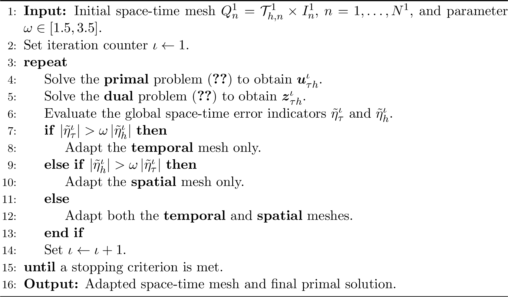
Remark 4 (Adaptation of the space-time mesh). In Algorithm 1, we do not specify the concrete marking strategy. We briefly describe the strategy used in this work.
Let \(\omega\in[1.5,3.5]\) be the criterion for temporal or spatial error domination. Let \(\theta_{\mathrm{top}}^\tau\in(0,1]\) denote the fraction of slabs to refine in time. Let \(\theta_{\mathrm{top},1}^{h,n},\theta_{\mathrm{top},2}^{h,n}\in(0,1]\) be the fractions of elements to refine on slab \(n\) without and with temporal refinement, respectively. Let \(\theta_{\mathrm{bot},1}^{h},\theta_{\mathrm{bot},2}^{h}\in[0,1)\) be the corresponding fractions of elements to coarsen.
Let \(\tilde{\eta}_\tau\) and \(\tilde{\eta}_h\) denote the global temporal and spatial indicators used for marking. The marking strategy is as follows.
If \(|\tilde{\eta}_\tau|\ge \omega\,|\tilde{\eta}_h|\), then we mark the top \(\theta_{\mathrm{top}}^\tau\) fraction of slabs for temporal refinement.
If \(|\tilde{\eta}_h|\ge \omega\,|\tilde{\eta}_\tau|\), then on each slab \(n\),
we refine the top \(\theta_{\mathrm{top},1}^{h,n}\) fraction of elements if the slab is not marked for temporal refinement,
we refine the top \(\theta_{\mathrm{top},2}^{h,n}\) fraction of elements if the slab is marked for temporal refinement,
we coarsen the bottom \(\theta_{\mathrm{bot},1}^{h}\) fraction of elements if the slab is not marked for temporal refinement,
we coarsen the bottom \(\theta_{\mathrm{bot},2}^{h}\) fraction of elements if the slab is marked for temporal refinement.
If neither indicator dominates, then we apply both the temporal and spatial marking rules above.
In Remark 4, we introduced slab-wise refinement fractions. In this work, we either keep these fractions constant, as in previous work, or adapt them according to the following rule.
Remark 5 (Slab-wise adaptation of the spatial refinement fractions). On iteration \(\iota\), define on each space-time slab the local indicator \[\tilde{\eta}_{\tau h}^{n,\iota}=\tilde{\eta}_{h}^{n,\iota}+\tilde{\eta}_{\tau}^{n,\iota}\,,\] and the corresponding global quantity \[\tilde{\eta}_{\tau h}^{\iota}=\sum_{n=1}^{N^\iota}\tilde{\eta}_{\tau h}^{n,\iota}\,.\] If \(\tilde{\eta}_{\tau h}^{\iota}=0\), we keep the nominal refinement fractions. Otherwise, we define the normalized slab-wise weights \[\alpha_n=\frac{\tilde{\eta}_{\tau h}^{n,\iota}}{\tilde{\eta}_{\tau h}^{\iota}}\,, \qquad \alpha_{\min}=\min_n\alpha_n\,, \qquad \alpha_{\max}=\max_n\alpha_n\,.\] These weights are used to adapt the nominal fraction \(\theta_{\mathrm{top},2}^{h}\) on slabs that are marked both in time and in space. To avoid large deviations from the nominal value, we bound the adapted fractions by \[\theta_{\mathrm{top},2}^{h,-}=\tfrac34\,\theta_{\mathrm{top},2}^{h}\,, \qquad \theta_{\mathrm{top},2}^{h,+}=\min\!\left\{1,\tfrac43\,\theta_{\mathrm{top},2}^{h}\right\}\,.\] The slab-wise fraction \(\theta_{\mathrm{top},2}^{h,n}\) is then defined by \[\theta_{\mathrm{top},2}^{h,n}= \begin{cases} \theta_{\mathrm{top},2}^{h}, & \alpha_{\max}-\alpha_{\min}<\varepsilon,\\[1ex] \displaystyle \theta_{\mathrm{top},2}^{h,-} +\bigl(\theta_{\mathrm{top},2}^{h,+}-\theta_{\mathrm{top},2}^{h,-}\bigr) \frac{\alpha_n-\alpha_{\min}}{\alpha_{\max}-\alpha_{\min}}, & \text{otherwise}, \end{cases}\] where \(\varepsilon>0\) is a small tolerance. Hence \[\theta_{\mathrm{top},2}^{h,n}\in \bigl[\theta_{\mathrm{top},2}^{h,-},\,\theta_{\mathrm{top},2}^{h,+}\bigr]\,,\] and the spatial refinement fraction is distributed according to the relative slab-wise error contributions.
Remark 6 (Dynamic meshes). We solve the fully problem 16 on the mesh slabs \(Q_n= \mathcal{T}_h^n \times I_n\). Here, the mesh \(\mathcal{T}_h^n\) and the pair of finite element spaces \(\boldsymbol{V}_h^k(\mathcal{T}_h^n)\times Q_h^{k-1}(\mathcal{T}_h^n)\) are allowed to change from subinterval to subinterval. The velocity field \(\boldsymbol{v}_{n-1}^{-}\coloneq \boldsymbol{v}_{\tau,h}(t_{n-1})\in \boldsymbol{V}_h^k(\mathcal{T}_h^{n-1})\), computed on \(I_{n-1}\), then satisfies the discrete divergence-free constraint with respect to all test functions in \(Q_h^{k-1}(\mathcal{T}_h^{n-1})\) and violates the constraint with respect to \(Q_h^{k-1}(\mathcal{T}_h^{n})\) on \(I_n\), if \(\mathcal{T}_h^{n-1}\neq \mathcal{T}_h^n\). To recover the discrete divergence-free constraint of the coupling term on \(I_n\), we substitute \(\boldsymbol{v}_{n-1}^{-}\) by its Helmholtz projection \(\Pi_h^n\boldsymbol{v}_{n-1}^{-}\in \boldsymbol{V}_h^k(\mathcal{T}_h^{n})\), satisfying with some additional pressure function \(\vartheta_h^n\in Q_h^{k-1}(\mathcal{T}_h^n)\) the variational equation [31], [39], \[\label{eq-stokes-projection} (\Pi_h^n\boldsymbol{v}_{n-1}^{-},\boldsymbol{v}_h) -(\vartheta_h^n,\nabla\cdot \boldsymbol{v}_h) +(\nabla\cdot \Pi_h^n\boldsymbol{v}_{n-1}^{-},q_h) = (\widehat{\boldsymbol{v}}_{\tau h,n-1}^{\,n},\boldsymbol{v}_h)\qquad{(1)}\] for all \((\boldsymbol{v}_h,q_h)\in \boldsymbol{V}_h^k(\mathcal{T}_h^n)\times Q_h^{k-1}(\mathcal{T}_h^n)\). The projection \(\Pi_h^n\boldsymbol{v}_{n-1}^{-}\in \boldsymbol{V}_h^k(\mathcal{T}_h^{n})\) is discretely divergence free with respect to the decomposition \(\mathcal{T}_h^n\) of \(\Omega\), \[(\nabla\cdot \Pi_h^n\boldsymbol{v}_{n-1}^{-},q_h)=0\] for all \(q_h\in Q_h^{k-1}(\mathcal{T}_h^n)\). Alternatively, a Stokes projection can be used. As studied in [31], either projections can lead to the accumulation of projection errors that are due to ?? . Instabilities and failure of can occur if arbitrary mesh modifications without hierarchical embeddings along with a high number of changes are involved. In our numerical computations presented in Section 5, we do not observe such shortcomings. Suitable space-time projections or further post-processing might overcome accumulating projection errors, even for high numbers of mesh changes.
4.3 Geometric Multigrid Preconditioned Newton-Krylov Method↩︎


The space-time finite element discretization of the incompressible Navier–Stokes equations leads to the nonlinear algebraic system 16 .
To solve this problem, we employ a Newton–Krylov method preconditioned by geometric multigrid. Newton’s method is applied in the weak form \[\label{newton} A_{\tau h}'(\boldsymbol{u}^{(l-1)})(\boldsymbol{w}^{(l)},\boldsymbol{\varphi}_{\tau h}) = F_{\tau h}(\boldsymbol{\varphi}_{\tau h}) - A_{\tau h}(\boldsymbol{u}^{(l-1)})(\boldsymbol{\varphi}_{\tau h}), \quad \boldsymbol{u}^{(l)}=\boldsymbol{u}^{(l-1)}+\boldsymbol{w}^{(l)}.\tag{41}\] Here \(A_{\tau h}'(\boldsymbol{u}^{(l-1)})\) denotes the Fréchet derivative of the semilinear form \(A_{\tau h}\) at \(\boldsymbol{u}^{(l-1)}\). Algebraically, this corresponds to the Jacobian matrix evaluated at \(\boldsymbol{u}^{(l-1)}\) and applied to the Newton correction \(\boldsymbol{w}^{(l)}\). The Jacobian can be computed analytically, see [8]. To reduce numerical costs, the Jacobian is reused over several Newton iterations and consecutive slabs, and is reassembled only when the observed residual reduction factor \(\|\boldsymbol{r}^{(l)}\|/\|\boldsymbol{r}^{(l-1)}\|\) exceeds a prescribed threshold \(\rho_{\max}\). In our computations, \(\rho_{\max}\) is chosen empirically and typically lies between \(0.05\) and \(0.1\).
Each Newton step requires the solution of a large, sparse, nonsymmetric, and indefinite linear system arising from the saddle-point structure of the Navier–Stokes equations. We use the Generalized Minimal Residual method (GMRES) [40], [41] to solve these linear systems. To accelerate convergence, GMRES is preconditioned by geometric multigrid. On each slab \(I_n\), the multigrid method is built on a hierarchy of nested discrete saddle-point spaces \[\mathcal{X}_0^n \subset \mathcal{X}_1^n \subset \cdots \subset \mathcal{X}_L^n,\] associated with nested spatial meshes \(\mathcal{T}_0^n,\dots,\mathcal{T}_L^n=\mathcal{T}_h^n\). On each level, high-frequency errors are damped by a smoothing operator, while low-frequency components are transferred to coarser levels by \(L^2\)-projection-based restriction and interpolative prolongation. On the coarsest level, a direct solver is employed. Under the standard multigrid assumptions, one V-cycle has linear complexity in the number of degrees of freedom.
To treat the saddle-point structure efficiently and to obtain a parallelizable smoother, we employ a Vanka-type smoother [42] within the multigrid cycle. It is defined by \[\label{vanka0} \mathcal{V}_\ell(A_\ell) = \sum_{K\in\mathcal{T}_\ell} R_K^\top \bigl[R_KA_\ell R_K^\top\bigr]^{-1}R_K,\tag{42}\] where \(A_\ell\) denotes the system matrix on level \(\ell\), and \(R_K\) is the restriction operator to the degrees of freedom associated with the element \(K\in\mathcal{T}_\ell\). One smoothing step is then given by \[\label{vanka} \mathcal{S}(\boldsymbol{A}_\ell,\boldsymbol{b}_\ell,\boldsymbol{x}_k) = \boldsymbol{x}_k + \omega\,\mathcal{V}_\ell(A_\ell)\, (\boldsymbol{b}_\ell-\boldsymbol{A}_\ell\boldsymbol{x}_k),\tag{43}\] with damping parameter \(\omega\in(0,1]\). In our experience, two to five pre- and post-smoothing steps are sufficient for robust convergence. The discontinuous pressure approximation is beneficial for the Vanka smoother, since it localizes the pressure degrees of freedom and thereby improves the efficiency of the element-wise local solves.
Remark 7 (Weighting in the Vanka smoother). In the implementation, the additive operator 42 is combined with a diagonal partition-of-unity weighting. We choose the weight of each degree of freedom as the reciprocal of its valence. An alternative is a restricted Vanka smoother, which assigns each degree of freedom to a unique element. This reduces communication, but in our tests it led to a less effective smoother and hence to a larger number of GMRES iterations. Since in the present matrix-based setting the dominant cost comes from global matrix-vector products, we use the weighted variant here.
Remark 8 (Dual linear systems). For fixed primal solution, the dual problem is linear and solved backward in time. Its slab-wise discretization leads to nonsymmetric saddle-point systems with diffusion, backward transport, and a reaction term. In the implementation, these systems are treated with the same GMRES-preconditioned geometric multigrid method as the primal Newton linearizations, based on the same level hierarchy, intergrid transfers, and Vanka-type smoothing.
In summary, the nonlinear space-time finite element system is linearized by Newton’s method and the resulting linear systems are solved by GMRES preconditioned by geometric multigrid with a Vanka-type smoother. For a more detailed description of the solver architecture and its parallelization, we refer to [22].
4.4 Parallel implementation↩︎
The implementation of the adaptive algorithm is distributed by MPI and uses the parallel infrastructure of deal.II for error estimation, marking, refinement, and multigrid setup across all processes. No stage is executed on a dedicated
master rank. Collective communication is still required for the assembly of global indicators and for the coarse-grid solve.
Remark 9 (MPI-distributed adaptation).
**Local error estimation with face terms.* Each rank computes its element-wise residual contributions, including jump terms on interior faces. For faces on process boundaries, ghost-element values are exchanged with neighboring ranks so that these face terms are evaluated consistently. Each face contribution is computed exactly once and communicated if necessary.*
**Global indicator assembly.* The local error contributions per slab or per element are summed by
MPI_Allreduceto form the global indicators \(\tilde{\eta}_h\) and \(\tilde{\eta}_\tau\), and to normalize the slab-wise weights \(\alpha_n\).***Marking for refinement and coarsening.* Each rank marks its locally owned slabs or elements according to the global decision between \(\tilde{\eta}_h\) and \(\tilde{\eta}_\tau\) and according to the local fractions \(\theta_{\mathrm{top},2}^{h,n}\). No additional communication is required for the marking itself.*
**Distributed mesh refinement.* At present, we do not repartition the mesh, so load imbalance may accumulate over several adaptive cycles. Repartitioning is available in
deal.II. In the present space-time setting, however, the many mesh transfers make it less clear how much performance can be gained. The development of an optimized repartitioning strategy is left to future work.***Multigrid preconditioner with local smoothing.* On each rank, the space-time element-wise Vanka smoother is applied to the locally owned elements on each level, with the usual ghost-layer exchange where required. The coarse-grid correction is handled by a global, direct solve.*
At present, load balancing and repartitioning are not used. To maintain scalability after several adaptive cycles, we plan to incorporate dynamic repartitioning in future work.
5 Numerical Examples↩︎
In this section, we investigate the performance properties of the proposed approach, which integrates goal-oriented error control with iterative solver techniques. In particular, we study the convergence behavior, computational efficiency, as well as stability properties of the underlying space-time adaptive algorithm (Algorithm 1) introduced in Sect. 4.2. These properties are examined by means of the following three numerical examples.
Exact Analytical Solution: The first example is an academic test problem including a given analytical solution that goes back to [5]. It is used to validate accuracy and efficiency of the derived approach for different discretizations up to polynomial order 3 in time and 4 in space.
DFG Benchmark 2D-3: The second example is the famous DFG flow around cylinder benchmark 2D-3 that simulates the time-periodic behavior of a fluid in a pipe with a circular obstacle that goes back to [43]. The goal functional is chosen to control the mean drag.
We evaluate the accuracy and efficiency of our proposed approach in terms of several quantities. Firstly, to assess the accuracy of the duality based space-time error estimator, we compute the effectivity index defined as the ratio of the estimated to the exact error, given by \[\label{eq:Ieff} I_{\mathrm{eff}}\coloneq \left|\frac{ \tilde{\eta}_{\tau} + \tilde{\eta}_{h}}{J(\boldsymbol{u})-J(\boldsymbol{u}_{\tau h})}\right|\,.\tag{44}\] Secondly, to measure the gain in accuracy over the increase of work, we determine the empirical convergence rates, averaged over all DWR-loops, \[\label{eq:mean-rates} \overline{\operatorname{rate}}_{N_{\mathrm{ST}}}^{\|e_T\|} \quad \text{and} \quad \overline{\operatorname{rate}}_{W_{\mathrm{tot}}}^{\|e_T\|}\tag{45}\] of the reduction of the error in the goal quantity with respect to the increase of the number of space-time degrees of freedom \(N_{\mathrm{ST}}\) and the total work \(W_{\mathrm{tot}}\). The latter is measured by the cumulative linear solver work \[\label{eq:work} W_{\mathrm{tot}} = W_p + W_d,\quad\text{with primal and dual contributions}\tag{46}\] \[W_p \coloneq \sum_{n=1}^{N_{\mathrm{time}}} n_{\mathrm{L},n}^{p} N_{\mathrm{DoF},n}^{p}, \; W_d \coloneq \sum_{n=1}^{N_{\mathrm{time}}} n_{\mathrm{L},n}^{d} N_{\mathrm{DoF},n}^{d}\,,\] where \(n_{\mathrm{L},n}^{p}\) and \(n_{\mathrm{L},n}^{d}\) denote the numbers of primal and dual linear iterations on slab \(Q_n = \mathcal{T}_h^n \times I_n\), and \(N_{\mathrm{DoF},n}^{p}\), \(N_{\mathrm{DoF},n}^{d}\) the corresponding numbers of spatial degrees of freedom. The nonlinear primal problem is solved by Newton’s method. We therefore also report the number of nonlinear iterations on slab \(Q_n\), denoted by \(n_{\mathrm{NL},n}\). Accordingly, we let \(n_{\mathrm{L},n}^{p}\) denote the total number of linear iterations accumulated over the \(n_{\mathrm{NL},n}\) Newton steps on slab \(Q_n\). By \(n_{\mathrm{NL}}\), \(n_{\mathrm{L}}^{p}\), and \(n_{\mathrm{L}}^{d}\) we denote the total numbers of nonlinear, primal linear, and dual linear iterations over all slabs within one DWR loop \(\ell\). In addition, we record \[\label{eq:iteration-indicators} \min_{\ell=1,\dots,\ell_{\max}} \Bigl(\frac{n_{\mathrm{NL}}}{N_{\mathrm{time}}}\Bigr),\;\; \max_{\ell=1,\dots,\ell_{\max}} \Bigl(\frac{n_{\mathrm{NL}}}{N_{\mathrm{time}}}\Bigr),\;\; \min_{\ell=1,\dots,\ell_{\max}} \Bigl(\frac{n_{\mathrm{L}}^{p}}{n_{\mathrm{NL}}}\Bigr),\;\; \max_{\ell=1,\dots,\ell_{\max}} \Bigl(\frac{n_{\mathrm{L}}^{p}}{n_{\mathrm{NL}}}\Bigr),\tag{47}\] together with the relative dual contribution \[\label{eq:dual-work-fraction} \frac{W_d}{W_{\mathrm{tot}}}.\tag{48}\] Throughout, by \(\ell\) we denote the refinement level or DWR loop number, \(N_{\text{time}}\) the number of subintervals in time, \(N_{\text{space}}^{\text{max}}\) the maximum number of degrees of freedom associated with a spatial triangulation within one loop and \(N_{\text{tot}}\) the number of total degrees of freedom in space and time. We consider different finite element approximations dG(\(r\))-\(Q_k/P_{k-1}^{\mathrm{disc}}\) denoting a discontinuous in time approximation of polynomial degree \(r\geq 0\) as well as a continuous velocity and discontinuous pressure approximations in space of polynomial degree \(k\geq2\).
The implementation is based on the deal.II finite element library [1]. The tests are run on a
single node with 2 Intel Xeon Platinum 8360Y CPUs and 1024 RAM of the HPC cluster HSUper at Helmut Schmidt University.
5.1 Example 1: Exact Analytical Solution↩︎
As a first test case, we consider a model problem on the space-time domain \(\Omega\times I = [0,1]^2\times [0, 1]\) with prescribed solution given for the velocity \(\boldsymbol{v} \colon \Omega\times I \to \mathbb{R}^2\) and pressure \(p \colon \Omega\times I \to \mathbb{R}\) by \[\label{eq:conv-test} \begin{align} \boldsymbol{v}(\boldsymbol{x},\,t) &= \sin(t) \begin{pmatrix} \sin^2(\pi x) \sin(\pi y) \cos(\pi y) \\ \sin(\pi x) \cos(\pi x) \sin^2(\pi y) \end{pmatrix}, \\ p(\boldsymbol{x},\,t) &= \sin(t) \sin(\pi x) \cos(\pi x) \sin(\pi y) \cos(\pi y)\,. \end{align}\tag{49}\] We choose the kinematic viscosity as \(\nu \in \{1, 10^{-3}\}\) and choose the external force \(\boldsymbol{f}\) such that the solution 49 satisfies 1 . The initial velocity is prescribed as zero and homogeneous Dirichlet boundary conditions are imposed on \(\partial\Omega\) for all times \[\boldsymbol{v} = \boldsymbol{0}\text{ on }\Omega\times \{0\},\quad \boldsymbol{v} = \boldsymbol{0}, \text{ on } \partial \Omega\times (0, T]\,.\] The initial space-time mesh \(\mathcal{T}_{h}\otimes\mathcal{M}_{\tau}\) is a uniform tensor-product partition of the space-time domain \(\Omega\times I\). We use discretizations with varying polynomial degrees \(r \in \{0,\dots,\,3\}\) in time, where we use \(\mathbb{Q}_{r+1}/\mathbb{P}_{r}^{\mathrm{disc}}\) elements in space, except for the \(dG(0)\) case where we use \(\mathbb{Q}_{2}/\mathbb{P}_{1}^{\mathrm{disc}}\) elements. The goal quantity is chosen to control the \(L^2\)-error \(e_N^-, e_N^-=u(\boldsymbol{x},T)-u_{\tau h}(T^{-})\), at the final time point \(T=1\), given by \[\label{eq:JL2final} J_T(u)= \frac{\big(u(\boldsymbol{x},T),e_N^-\big)}{\|e_N^-\|}\,.\tag{50}\] In Tables ¿tbl:tab:dG0?–¿tbl:tab:dG3? we present the development of the total discretization error \(J(e)=\|e_T\|\), the approximated spatial and temporal error estimators \(\eta_h\) and \(\eta_\tau\) as well as the effectivity index \(I_{\mathrm{eff}}\) during an adaptive refinement process for various discretizations. For all discretizations considered, we observe a consistent and satisfactory reduction of the discretization error \(\|e_T\|\). Concerning the accuracy of the employed error estimators, all cases exhibit reliable quantitative agreement with the discretization error, as indicated by effectivity indices \(I_{\mathrm{eff}}\) close to one (cf. the last column of Tables ¿tbl:tab:dG0?–¿tbl:tab:dG3?). From the perspective of computational efficiency in space–time adaptive algorithms, it is crucial to ensure an equilibrated reduction of the temporal as well as spatial discretization error. Referring to this, we point out for all test cases a good equilibration of the spatial and temporal error indicators \(\eta_h\) and \(\eta_\tau\) in the course of the refinement process (cf. column 6 and 7 of Tables ¿tbl:tab:dG0?–¿tbl:tab:dG3?).
5.5pt
8pt
| 1 | 5 | 210 | 1050 | 2.2017e-02 | 1.9422e-03 | 1.0825e-02 | 1.2767e-02 | 0.57989 | |||||||||||||||||||||||||||||||||||||||||||||||||||||||||||||||||||||||||||||||||||||||||||||||||||||||||||||||||||||||||||||||||||||||||||||||||||||||||||||||||||||||||||||||||||||||||||||||||||||||||||||||||||||||||||||||||||||||||||||||||||||||||||||||||||||||||||||||||||||||||||||||||||||||||||||||||||||||||||||||||||||||||||||||||||||||||||
| 2 | 6 | 374 | 2680 | 1.0655e-02 | 4.6144e-03 | 6.2266e-03 | 1.0841e-02 | 1.0175 | |||||||||||||||||||||||||||||||||||||||||||||||||||||||||||||||||||||||||||||||||||||||||||||||||||||||||||||||||||||||||||||||||||||||||||||||||||||||||||||||||||||||||||||||||||||||||||||||||||||||||||||||||||||||||||||||||||||||||||||||||||||||||||||||||||||||||||||||||||||||||||||||||||||||||||||||||||||||||||||||||||||||||||||||||||||||||||
| 3 | 7 | 592 | 4766 | 5.1732e-03 | 1.1152e-03 | 4.0802e-03 | 5.1954e-03 | 1.0043 | |||||||||||||||||||||||||||||||||||||||||||||||||||||||||||||||||||||||||||||||||||||||||||||||||||||||||||||||||||||||||||||||||||||||||||||||||||||||||||||||||||||||||||||||||||||||||||||||||||||||||||||||||||||||||||||||||||||||||||||||||||||||||||||||||||||||||||||||||||||||||||||||||||||||||||||||||||||||||||||||||||||||||||||||||||||||||||
| 4 | 9 | 623 | 11069 | 2.6679e-03 | 1.5040e-03 | 2.1946e-03 | 3.6986e-03 | 1.3863 | |||||||||||||||||||||||||||||||||||||||||||||||||||||||||||||||||||||||||||||||||||||||||||||||||||||||||||||||||||||||||||||||||||||||||||||||||||||||||||||||||||||||||||||||||||||||||||||||||||||||||||||||||||||||||||||||||||||||||||||||||||||||||||||||||||||||||||||||||||||||||||||||||||||||||||||||||||||||||||||||||||||||||||||||||||||||||||
| 5 | 11 | 703 | 21704 | 1.5606e-03 | 1.0923e-03 | 1.4662e-03 | 2.5585e-03 | 1.6395 | |||||||||||||||||||||||||||||||||||||||||||||||||||||||||||||||||||||||||||||||||||||||||||||||||||||||||||||||||||||||||||||||||||||||||||||||||||||||||||||||||||||||||||||||||||||||||||||||||||||||||||||||||||||||||||||||||||||||||||||||||||||||||||||||||||||||||||||||||||||||||||||||||||||||||||||||||||||||||||||||||||||||||||||||||||||||||||
| 6 | 14 | 761 | 40028 | 9.7239e-04 | 6.4904e-04 | 9.5853e-04 | 1.6076e-03 | 1.6532 | |||||||||||||||||||||||||||||||||||||||||||||||||||||||||||||||||||||||||||||||||||||||||||||||||||||||||||||||||||||||||||||||||||||||||||||||||||||||||||||||||||||||||||||||||||||||||||||||||||||||||||||||||||||||||||||||||||||||||||||||||||||||||||||||||||||||||||||||||||||||||||||||||||||||||||||||||||||||||||||||||||||||||||||||||||||||||||
| 7 | 18 | 11761 | 91930 | 6.4359e-04 | 3.4885e-04 | 6.6339e-04 | 1.0122e-03 | 1.5728 | |||||||||||||||||||||||||||||||||||||||||||||||||||||||||||||||||||||||||||||||||||||||||||||||||||||||||||||||||||||||||||||||||||||||||||||||||||||||||||||||||||||||||||||||||||||||||||||||||||||||||||||||||||||||||||||||||||||||||||||||||||||||||||||||||||||||||||||||||||||||||||||||||||||||||||||||||||||||||||||||||||||||||||||||||||||||||||
| 8 | 23 | 15203 | 193063 | 4.4344e-04 | 1.4049e-04 | 4.4870e-04 | 5.8919e-04 | 1.3287 | |||||||||||||||||||||||||||||||||||||||||||||||||||||||||||||||||||||||||||||||||||||||||||||||||||||||||||||||||||||||||||||||||||||||||||||||||||||||||||||||||||||||||||||||||||||||||||||||||||||||||||||||||||||||||||||||||||||||||||||||||||||||||||||||||||||||||||||||||||||||||||||||||||||||||||||||||||||||||||||||||||||||||||||||||||||||||||
| 9 | 29 | 15489 | 439491 | 3.2443e-04 | 8.0905e-05 | 3.3948e-04 | 4.2039e-04 | 1.2958 | |||||||||||||||||||||||||||||||||||||||||||||||||||||||||||||||||||||||||||||||||||||||||||||||||||||||||||||||||||||||||||||||||||||||||||||||||||||||||||||||||||||||||||||||||||||||||||||||||||||||||||||||||||||||||||||||||||||||||||||||||||||||||||||||||||||||||||||||||||||||||||||||||||||||||||||||||||||||||||||||||||||||||||||||||||||||||||
| 10 | 37 | 15187 | 869234 | 2.3714e-04 | 6.5660e-05 | 2.4683e-04 | 3.1249e-04 | 1.3177 | |||||||||||||||||||||||||||||||||||||||||||||||||||||||||||||||||||||||||||||||||||||||||||||||||||||||||||||||||||||||||||||||||||||||||||||||||||||||||||||||||||||||||||||||||||||||||||||||||||||||||||||||||||||||||||||||||||||||||||||||||||||||||||||||||||||||||||||||||||||||||||||||||||||||||||||||||||||||||||||||||||||||||||||||||||||||||||
| 11 | 48 | 17776 | 1698684 | 1.7576e-04 | 4.3620e-05 | 1.8111e-04 | 2.2473e-04 | 1.2786 | |||||||||||||||||||||||||||||||||||||||||||||||||||||||||||||||||||||||||||||||||||||||||||||||||||||||||||||||||||||||||||||||||||||||||||||||||||||||||||||||||||||||||||||||||||||||||||||||||||||||||||||||||||||||||||||||||||||||||||||||||||||||||||||||||||||||||||||||||||||||||||||||||||||||||||||||||||||||||||||||||||||||||||||||||||||||||||
| 12 | 62 | 26742 | 3599510 | 1.2984e-04 | 3.5041e-05 | 1.3323e-04 | 1.6827e-04 | 1.2960 | |||||||||||||||||||||||||||||||||||||||||||||||||||||||||||||||||||||||||||||||||||||||||||||||||||||||||||||||||||||||||||||||||||||||||||||||||||||||||||||||||||||||||||||||||||||||||||||||||||||||||||||||||||||||||||||||||||||||||||||||||||||||||||||||||||||||||||||||||||||||||||||||||||||||||||||||||||||||||||||||||||||||||||||||||||||||||||
| 13 | 80 | 21531 | 7238636 | 9.8363e-05 | 2.2881e-05 | 1.0141e-04 | 1.2430e-04 | 1.2636 |
4.5pt
8pt
| 1 | 4 | 1540 | 6160 | 9.3412e-04 | 2.8871e-04 | 6.7677e-05 | 3.5639e-04 | 0.38 | |||||||||||||||||||||||||||||||||||||||||||||||||||||||||||||||||||||||||||||||||||||||||||||||||||||||||||||||||||||||||||||||||||||||||||||||||||||||||||||||||||||||||||||||||||||||||||||||||||||||||||||||||||||||||||||||||||||||||||||||||||||||||||||||||||||||||||||||||||||||||||||||||||||||||||||||||||||||||||||||||||||||||||||||||||||||||||
| 2 | 5 | 1736 | 12390 | 4.5738e-04 | 3.1714e-04 | 4.0001e-05 | 3.5714e-04 | 0.78 | |||||||||||||||||||||||||||||||||||||||||||||||||||||||||||||||||||||||||||||||||||||||||||||||||||||||||||||||||||||||||||||||||||||||||||||||||||||||||||||||||||||||||||||||||||||||||||||||||||||||||||||||||||||||||||||||||||||||||||||||||||||||||||||||||||||||||||||||||||||||||||||||||||||||||||||||||||||||||||||||||||||||||||||||||||||||||||
| 3 | 5 | 3248 | 23138 | 2.1601e-04 | -7.3945e-05 | 1.9074e-05 | -5.4871e-05 | 0.25 | |||||||||||||||||||||||||||||||||||||||||||||||||||||||||||||||||||||||||||||||||||||||||||||||||||||||||||||||||||||||||||||||||||||||||||||||||||||||||||||||||||||||||||||||||||||||||||||||||||||||||||||||||||||||||||||||||||||||||||||||||||||||||||||||||||||||||||||||||||||||||||||||||||||||||||||||||||||||||||||||||||||||||||||||||||||||||||
| 4 | 7 | 3494 | 57272 | 9.1844e-05 | -4.3569e-06 | 4.4129e-06 | 5.5998e-08 | 0.00061 | |||||||||||||||||||||||||||||||||||||||||||||||||||||||||||||||||||||||||||||||||||||||||||||||||||||||||||||||||||||||||||||||||||||||||||||||||||||||||||||||||||||||||||||||||||||||||||||||||||||||||||||||||||||||||||||||||||||||||||||||||||||||||||||||||||||||||||||||||||||||||||||||||||||||||||||||||||||||||||||||||||||||||||||||||||||||||||
| 5 | 9 | 3572 | 114154 | 5.1669e-05 | 5.9771e-05 | 6.6503e-06 | 6.6421e-05 | 1.29 | |||||||||||||||||||||||||||||||||||||||||||||||||||||||||||||||||||||||||||||||||||||||||||||||||||||||||||||||||||||||||||||||||||||||||||||||||||||||||||||||||||||||||||||||||||||||||||||||||||||||||||||||||||||||||||||||||||||||||||||||||||||||||||||||||||||||||||||||||||||||||||||||||||||||||||||||||||||||||||||||||||||||||||||||||||||||||||
| 6 | 9 | 4712 | 183120 | 2.5171e-05 | 8.6274e-06 | 2.3658e-06 | 1.0993e-05 | 0.44 | |||||||||||||||||||||||||||||||||||||||||||||||||||||||||||||||||||||||||||||||||||||||||||||||||||||||||||||||||||||||||||||||||||||||||||||||||||||||||||||||||||||||||||||||||||||||||||||||||||||||||||||||||||||||||||||||||||||||||||||||||||||||||||||||||||||||||||||||||||||||||||||||||||||||||||||||||||||||||||||||||||||||||||||||||||||||||||
| 7 | 12 | 4868 | 371674 | 1.0561e-05 | 9.7207e-06 | 3.2539e-07 | 1.0046e-05 | 0.95 | |||||||||||||||||||||||||||||||||||||||||||||||||||||||||||||||||||||||||||||||||||||||||||||||||||||||||||||||||||||||||||||||||||||||||||||||||||||||||||||||||||||||||||||||||||||||||||||||||||||||||||||||||||||||||||||||||||||||||||||||||||||||||||||||||||||||||||||||||||||||||||||||||||||||||||||||||||||||||||||||||||||||||||||||||||||||||||
| 8 | 12 | 4868 | 655942 | 6.2456e-06 | 3.8154e-06 | 4.4631e-07 | 4.2617e-06 | 0.68 | |||||||||||||||||||||||||||||||||||||||||||||||||||||||||||||||||||||||||||||||||||||||||||||||||||||||||||||||||||||||||||||||||||||||||||||||||||||||||||||||||||||||||||||||||||||||||||||||||||||||||||||||||||||||||||||||||||||||||||||||||||||||||||||||||||||||||||||||||||||||||||||||||||||||||||||||||||||||||||||||||||||||||||||||||||||||||||
| 9 | 12 | 129014 | 1180326 | 2.7837e-06 | -3.4125e-06 | 3.9546e-07 | -3.0170e-06 | 1.08 |
4.5pt
8pt
| 1 | 2 | 4902 | 9804 | 1.7087e-04 | 2.9316e-06 | 4.3518e-05 | 4.6450e-05 | 0.27184 | |||||||||||||||||||||||||||||||||||||||||||||||||||||||||||||||||||||||||||||||||||||||||||||||||||||||||||||||||||||||||||||||||||||||||||||||||||||||||||||||||||||||||||||||||||||||||||||||||||||||||||||||||||||||||||||||||||||||||||||||||||||||||||||||||||||||||||||||||||||||||||||||||||||||||||||||||||||||||||||||||||||||||||||||||||||||||||
| 2 | 3 | 4902 | 14706 | 3.4100e-05 | 1.5325e-05 | 1.5867e-06 | 1.6912e-05 | 0.49595 | |||||||||||||||||||||||||||||||||||||||||||||||||||||||||||||||||||||||||||||||||||||||||||||||||||||||||||||||||||||||||||||||||||||||||||||||||||||||||||||||||||||||||||||||||||||||||||||||||||||||||||||||||||||||||||||||||||||||||||||||||||||||||||||||||||||||||||||||||||||||||||||||||||||||||||||||||||||||||||||||||||||||||||||||||||||||||||
| 3 | 3 | 19920 | 61122 | 1.9126e-05 | 6.5756e-05 | 2.9991e-06 | 6.8755e-05 | 3.5949 | |||||||||||||||||||||||||||||||||||||||||||||||||||||||||||||||||||||||||||||||||||||||||||||||||||||||||||||||||||||||||||||||||||||||||||||||||||||||||||||||||||||||||||||||||||||||||||||||||||||||||||||||||||||||||||||||||||||||||||||||||||||||||||||||||||||||||||||||||||||||||||||||||||||||||||||||||||||||||||||||||||||||||||||||||||||||||||
| 4 | 3 | 40368 | 128460 | 1.6319e-05 | 4.7500e-05 | 3.5835e-06 | 5.1084e-05 | 3.1303 | |||||||||||||||||||||||||||||||||||||||||||||||||||||||||||||||||||||||||||||||||||||||||||||||||||||||||||||||||||||||||||||||||||||||||||||||||||||||||||||||||||||||||||||||||||||||||||||||||||||||||||||||||||||||||||||||||||||||||||||||||||||||||||||||||||||||||||||||||||||||||||||||||||||||||||||||||||||||||||||||||||||||||||||||||||||||||||
| 5 | 3 | 121374 | 399990 | 1.4557e-05 | 1.4939e-05 | 4.0396e-06 | 1.8979e-05 | 1.3038 | |||||||||||||||||||||||||||||||||||||||||||||||||||||||||||||||||||||||||||||||||||||||||||||||||||||||||||||||||||||||||||||||||||||||||||||||||||||||||||||||||||||||||||||||||||||||||||||||||||||||||||||||||||||||||||||||||||||||||||||||||||||||||||||||||||||||||||||||||||||||||||||||||||||||||||||||||||||||||||||||||||||||||||||||||||||||||||
| 6 | 4 | 137706 | 782160 | 1.0120e-06 | 6.7099e-06 | 1.8632e-07 | 6.8962e-06 | 6.8141 | |||||||||||||||||||||||||||||||||||||||||||||||||||||||||||||||||||||||||||||||||||||||||||||||||||||||||||||||||||||||||||||||||||||||||||||||||||||||||||||||||||||||||||||||||||||||||||||||||||||||||||||||||||||||||||||||||||||||||||||||||||||||||||||||||||||||||||||||||||||||||||||||||||||||||||||||||||||||||||||||||||||||||||||||||||||||||||
| 7 | 4 | 234618 | 1229250 | 9.5143e-07 | 3.5681e-06 | 1.9791e-07 | 3.7660e-06 | 3.9583 | |||||||||||||||||||||||||||||||||||||||||||||||||||||||||||||||||||||||||||||||||||||||||||||||||||||||||||||||||||||||||||||||||||||||||||||||||||||||||||||||||||||||||||||||||||||||||||||||||||||||||||||||||||||||||||||||||||||||||||||||||||||||||||||||||||||||||||||||||||||||||||||||||||||||||||||||||||||||||||||||||||||||||||||||||||||||||||
| 8 | 4 | 704400 | 3852132 | 9.1104e-07 | 1.3522e-06 | 2.0716e-07 | 1.5593e-06 | 1.7116 | |||||||||||||||||||||||||||||||||||||||||||||||||||||||||||||||||||||||||||||||||||||||||||||||||||||||||||||||||||||||||||||||||||||||||||||||||||||||||||||||||||||||||||||||||||||||||||||||||||||||||||||||||||||||||||||||||||||||||||||||||||||||||||||||||||||||||||||||||||||||||||||||||||||||||||||||||||||||||||||||||||||||||||||||||||||||||||
| 9 | 4 | 1106778 | 6574092 | 9.0892e-07 | 8.4627e-07 | 2.0766e-07 | 1.0539e-06 | 1.1595 |
4.5pt
8pt
| 1 | 2 | 11272 | 22544 | 4.6212e-06 | 1.8080e-07 | 4.3643e-07 | 6.1723e-07 | 0.13 | |||||||||||||||||||||||||||||||||||||||||||||||||||||||||||||||||||||||||||||||||||||||||||||||||||||||||||||||||||||||||||||||||||||||||||||||||||||||||||||||||||||||||||||||||||||||||||||||||||||||||||||||||||||||||||||||||||||||||||||||||||||||||||||||||||||||||||||||||||||||||||||||||||||||||||||||||||||||||||||||||||||||||||||||||||||||||||
| 2 | 3 | 18664 | 78888 | 7.6425e-07 | -5.3932e-07 | 5.3089e-09 | -5.3401e-07 | 0.70 | |||||||||||||||||||||||||||||||||||||||||||||||||||||||||||||||||||||||||||||||||||||||||||||||||||||||||||||||||||||||||||||||||||||||||||||||||||||||||||||||||||||||||||||||||||||||||||||||||||||||||||||||||||||||||||||||||||||||||||||||||||||||||||||||||||||||||||||||||||||||||||||||||||||||||||||||||||||||||||||||||||||||||||||||||||||||||||
| 3 | 3 | 38536 | 157424 | 3.3388e-07 | -4.0245e-07 | 1.4767e-08 | -3.8769e-07 | 1.16 | |||||||||||||||||||||||||||||||||||||||||||||||||||||||||||||||||||||||||||||||||||||||||||||||||||||||||||||||||||||||||||||||||||||||||||||||||||||||||||||||||||||||||||||||||||||||||||||||||||||||||||||||||||||||||||||||||||||||||||||||||||||||||||||||||||||||||||||||||||||||||||||||||||||||||||||||||||||||||||||||||||||||||||||||||||||||||||
| 4 | 3 | 53528 | 277208 | 1.7752e-07 | -2.6782e-07 | 2.2228e-08 | -2.4559e-07 | 1.38 | |||||||||||||||||||||||||||||||||||||||||||||||||||||||||||||||||||||||||||||||||||||||||||||||||||||||||||||||||||||||||||||||||||||||||||||||||||||||||||||||||||||||||||||||||||||||||||||||||||||||||||||||||||||||||||||||||||||||||||||||||||||||||||||||||||||||||||||||||||||||||||||||||||||||||||||||||||||||||||||||||||||||||||||||||||||||||||
| 5 | 3 | 62944 | 450472 | 1.7548e-07 | -2.9604e-07 | 2.2457e-08 | -2.7359e-07 | 1.56 | |||||||||||||||||||||||||||||||||||||||||||||||||||||||||||||||||||||||||||||||||||||||||||||||||||||||||||||||||||||||||||||||||||||||||||||||||||||||||||||||||||||||||||||||||||||||||||||||||||||||||||||||||||||||||||||||||||||||||||||||||||||||||||||||||||||||||||||||||||||||||||||||||||||||||||||||||||||||||||||||||||||||||||||||||||||||||||
| 6 | 3 | 113528 | 596728 | 1.7485e-07 | -1.9283e-07 | 2.2517e-08 | -1.7032e-07 | 0.97 | |||||||||||||||||||||||||||||||||||||||||||||||||||||||||||||||||||||||||||||||||||||||||||||||||||||||||||||||||||||||||||||||||||||||||||||||||||||||||||||||||||||||||||||||||||||||||||||||||||||||||||||||||||||||||||||||||||||||||||||||||||||||||||||||||||||||||||||||||||||||||||||||||||||||||||||||||||||||||||||||||||||||||||||||||||||||||||
| 7 | 4 | 225000 | 1958424 | 6.1465e-09 | -6.62e-09 | 4.36e-10 | -6.1870e-09 | 1.01 | |||||||||||||||||||||||||||||||||||||||||||||||||||||||||||||||||||||||||||||||||||||||||||||||||||||||||||||||||||||||||||||||||||||||||||||||||||||||||||||||||||||||||||||||||||||||||||||||||||||||||||||||||||||||||||||||||||||||||||||||||||||||||||||||||||||||||||||||||||||||||||||||||||||||||||||||||||||||||||||||||||||||||||||||||||||||||||
| 8 | 4 | 284728 | 2768280 | 4.3765e-09 | -6.89e-09 | 6.13e-10 | -6.2785e-09 | 1.43 |
Across all four fully adaptive runs, the DWR estimator in combination with adaptive refinement yields a consistent reduction of the goal error with increasing space-time resolution, while the corresponding effectivity indices remain in a reasonable range. The reported mean rates show that the decay of the goal error with respect to total work is close to its decay with respect to the space-time number of degrees of freedom, indicating that the adaptive refinement translates effectively into computational efficiency. A compact comparison of these approximation and cost quantities is given in Table 1.
| DWR | mean rates | \(n_{\mathrm{NL}}/N_{\mathrm{time}}\) | \(n_{\mathrm{L}}^{p}/n_{\mathrm{NL}}\) | |||||||||||||||||||||||||||||||||||||||||||||||||||||||||||||||||||||||||||||||||||||||||||||||||||||||||||||||||||||||||||||||||||||||||||||||||||||||||||||||||||||||||||||||||||||||||||||||||||||||||||||||||||||||||||||||||||||||||||||||||||||||||||||||||||||||||||||||||||||||||||||||||||||||||||||||||||||||||||||||||||||||||||||||||||||||||||||||||||||||||||||||||||||||||||||||||||||||||||||||||||||||||||||||||||||||||||||||||||||||||||||
| \(N_{\mathrm{ST}}\) | \(I_{\mathrm{eff}}\) | \(\overline{\operatorname{rate}}_{W_{\mathrm{tot}}}^{\|e_T\|}\) | \(\max\) | \(\max\) | ||||||||||||||||||||||||||||||||||||||||||||||||||||||||||||||||||||||||||||||||||||||||||||||||||||||||||||||||||||||||||||||||||||||||||||||||||||||||||||||||||||||||||||||||||||||||||||||||||||||||||||||||||||||||||||||||||||||||||||||||||||||||||||||||||||||||||||||||||||||||||||||||||||||||||||||||||||||||||||||||||||||||||||||||||||||||||||||||||||||||||||||||||||||||||||||||||||||||||||||||||||||||||||||||||||||||||||||||||||||||||||
| 0 | 13 | 7238636 | 9.84e-05 | 1.24e-04 | 1.26 | 0.62 | 0.50 | 2.8 | 3.44 | 1.0 | 13.52 | 0.37 | ||||||||||||||||||||||||||||||||||||||||||||||||||||||||||||||||||||||||||||||||||||||||||||||||||||||||||||||||||||||||||||||||||||||||||||||||||||||||||||||||||||||||||||||||||||||||||||||||||||||||||||||||||||||||||||||||||||||||||||||||||||||||||||||||||||||||||||||||||||||||||||||||||||||||||||||||||||||||||||||||||||||||||||||||||||||||||||||||||||||||||||||||||||||||||||||||||||||||||||||||||||||||||||||||||||||||||||||||||||
| 1 | 9 | 1180326 | 2.78e-06 | 3.02e-06 | 1.08 | 1.13 | 0.99 | 3.0 | 3.50 | 8.42 | 17.69 | 0.28 | ||||||||||||||||||||||||||||||||||||||||||||||||||||||||||||||||||||||||||||||||||||||||||||||||||||||||||||||||||||||||||||||||||||||||||||||||||||||||||||||||||||||||||||||||||||||||||||||||||||||||||||||||||||||||||||||||||||||||||||||||||||||||||||||||||||||||||||||||||||||||||||||||||||||||||||||||||||||||||||||||||||||||||||||||||||||||||||||||||||||||||||||||||||||||||||||||||||||||||||||||||||||||||||||||||||||||||||||||||||
| 2 | 9 | 6574092 | 9.09e-07 | 1.05e-06 | 1.16 | 1.11 | 1.12 | 3.0 | 3.33 | 11.5 | 21.62 | 0.31 | ||||||||||||||||||||||||||||||||||||||||||||||||||||||||||||||||||||||||||||||||||||||||||||||||||||||||||||||||||||||||||||||||||||||||||||||||||||||||||||||||||||||||||||||||||||||||||||||||||||||||||||||||||||||||||||||||||||||||||||||||||||||||||||||||||||||||||||||||||||||||||||||||||||||||||||||||||||||||||||||||||||||||||||||||||||||||||||||||||||||||||||||||||||||||||||||||||||||||||||||||||||||||||||||||||||||||||||||||||||
| 3 | 8 | 2768280 | 4.38e-09 | 6.28e-09 | 1.43 | 1.08 | 0.98 | 3.0 | 3.33 | 14.17 | 24.17 | 0.31 | ||||||||||||||||||||||||||||||||||||||||||||||||||||||||||||||||||||||||||||||||||||||||||||||||||||||||||||||||||||||||||||||||||||||||||||||||||||||||||||||||||||||||||||||||||||||||||||||||||||||||||||||||||||||||||||||||||||||||||||||||||||||||||||||||||||||||||||||||||||||||||||||||||||||||||||||||||||||||||||||||||||||||||||||||||||||||||||||||||||||||||||||||||||||||||||||||||||||||||||||||||||||||||||||||||||||||||||||||||||
The algebraic behavior is summarized in Figure 4, which shows stable nonlinear iteration counts per slab and only moderate growth of the primal linear iterations per nonlinear step over the adaptive loops. This indicates that the slab-wise geometric multigrid preconditioned Newton–Krylov method remains robust under successive adaptive refinement. At the same time, the relative dual work fraction stays at a comparable level across all discretizations, showing that the adjoint solve contributes a noticeable but controlled part of the overall computational cost.
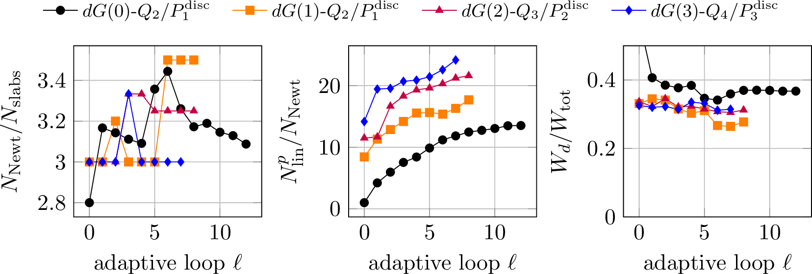
In Fig. 5 we plot the share of the primal problem, the dual problem as well as the error estimation over the entire wallclock time and its percentage share for one adaptive run including all DWR loops for the different discretizations corresponding to Tables ¿tbl:tab:dG0?–¿tbl:tab:dG3?. While the total runtime from dG(\(1\))-\(Q_2/P_1^{\textrm{disc}}\) to dG(\(3\))-\(Q_4/P_3^{\textrm{disc}}\) increases progressively as expected, the percentage share of the three units remains stable and nearly unchanged across all discretizations. In comparison to the primal problem, the dual problem requires only one third of its computational effort, while the error estimator itself is negligible at less than one percent. The fact that the total runtime of the dG(\(0\))-\(Q_2/P_1^{\textrm{disc}}\) discretization is slightly higher to that of the dG(\(1\))-\(Q_2/P_1^{\textrm{disc}}\) one is due to the large number of slabs required in the first case.
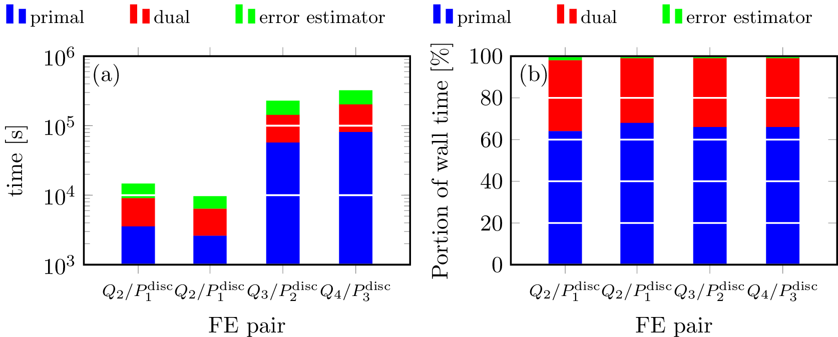
Finally, in Fig. 6 and Fig. 7 we visualize the distribution of the adaptively determined time step sizes \(\tau_n\) and minimal spatial element diameter \(\min_{K\in\mathcal{T}_h^{n,\ell_{\max}}} h_K\) within the slab \(Q_n\) over the entire time interval \(I\), respectively, corresponding to the final DWR loop of the different discretizations listed in Tables ¿tbl:tab:dG0?–¿tbl:tab:dG3?. For all discretizations, the step and element sizes are relatively large at the beginning, but they decrease continuously over time, reaching their minimal values at the final time \(T=1\). We note that the initial steps correspond to the initial distribution of the temporal and spatial meshes. This behavior is consistent with the choice of the underlying goal functional 50 , which specifically targets the control of the \(L^2\)-error at the final time \(T\). Furthermore, we observe that the total length of the subintervals is significantly reduced when using higher-order discretizations compared to the lowest-order case.
![Figure 6: Distribution of the adaptively determined temporal step size \tau_n plotted over the entire time interval I=(0,T] for the different discretizations corresponding to the respective final DWR loop inTables ¿tbl:tab:dG0?–¿tbl:tab:dG3?.](/article/2607.00686/_pdflatex/csfiapkj.png "fig:")
![Figure 7: Distribution of the adaptively determined minimal spatial element diameter \min_{K\in\mathcal{T}_h^{n,\ell_{\max}}} h_K within the slab Q_n plotted over the entire time interval I=(0,T] for the different discretizations corresponding to the respective final DWR loop inTables ¿tbl:tab:dG0?–¿tbl:tab:dG3?.](/article/2607.00686/_pdflatex/yxksfvdb.png "fig:")
5.2 Example 2: DFG Benchmark 2D-3↩︎
We consider the well-established benchmark problem of laminar flow around a cylinder introduced by Schäfer and Turek [43], precisely the unsteady 2D-3 test setting. In this case, the flow around a circular obstacle with Reynolds number \(\mathrm{Re}=100\) (the kinematic viscosity is set to \(\nu=0.001\)) is driven by a parabolic inflow profile whose amplitude is modulated in time by a \(\sin\) function. The geometry of the flow domain is shown in Fig. 8. We note that the coarse mesh used here is the same as in previous studies [5], [44]. The final time point is set to \(T=8\). The goal quantity is chosen to control the error of the mean drag coefficient. This coefficient is defined by \[\label{eq:Jmeandrag} J_{\textrm{drag}}(u)= \displaystyle-\int_I\{(\partial_t\boldsymbol{v},\hat{\boldsymbol{\psi}}_d)+a(\boldsymbol{u})(\hat{\boldsymbol{\varphi}}_d)\}\,\mathrm{d}t\,,\tag{51}\] where \(\hat{\boldsymbol{\varphi}}_d=(\hat{\boldsymbol{\psi}}_d,0)^\top\) fulfills \(\hat{\boldsymbol{\psi}}_d|_S=(|I|^{-1}C,0)^\top\,, \;\; \hat{\boldsymbol{\psi}}_d|_{\partial\Omega\textbackslash S}=\boldsymbol{0}\) with the constant \(C=2(U_{\mathrm{mean}}^2d)^{-1}\). Here, the mean inflow velocity is given by \[U_{\mathrm{mean}}=2/3\;\boldsymbol{v}_D(0,0.205,0)=\sin (\pi t/8)\] given by Eq. 52 and \(d\) denotes the diameter of the obstacle with boundary \(S=S=\partial B_r(0.2,0.2)\). We take the reference value for the goal functional from [5] and set it to 1.6072872.
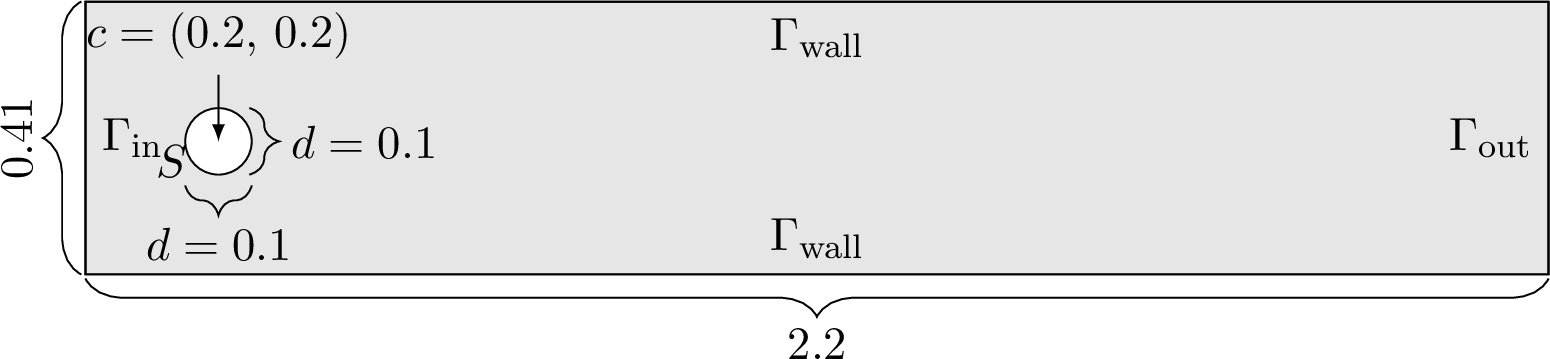
The flow is driven by the Dirichlet inflow profile \(\boldsymbol{v}=\boldsymbol{v}_D\) on the left boundary \(\Gamma_{\mathrm{in}} \coloneq \{0\}\times[0,H],\) given by \[\label{eq:inflow} \boldsymbol{v}_D(\boldsymbol{x},t) = \begin{pmatrix} \sin\!\left(\frac{\pi}{8}t\right)\dfrac{6y(H-y)}{H^2}\\[0.3em] 0 \end{pmatrix} \qquad \text{on }\Gamma_{\mathrm{in}},\tag{52}\] where \(H=0.41\) denotes the channel height. On the wall boundary \(\Gamma_{\mathrm{wall}}\) and on the obstacle boundary we prescribe no-slip boundary conditions \(\boldsymbol{v}=\boldsymbol{0}\). On the outflow boundary \(\Gamma_{\mathrm{out}}\) we impose a do-nothing condition [27].
In Table ¿tbl:tab:dfg-drag-all? we present the results of an adaptive refinement run together with a comparison of the algebraic performance of a GMG-preconditioned Newton-Krylov method and an ILU method using a dG(\(1\))-\(Q_2/P_1^{\mathrm{disc}}\) discretization. The adaptive refinement reduces the mean drag error 51 monotonically. The drag value converges to the reference value and the effectivity indices stay close to one on all loops. This shows that the DWR estimator provides a reliable approximation of the goal error. The observed decay of the goal error with respect to the space-time number of degrees of freedom is at least linear and becomes higher on the finer loops. Measured against total algebraic work, the same trend is obtained more efficiently with GMG than with ILU.
| 1 | 160 | 606720 | 1.389 | 2.137e-01 | 1.565e-01 | 9.082e-02 | 2.473e-01 | 1.1571 | |||||||||||||||||||||||||||||||||||||||||||||||||||||||||||||||||||||||||||||||||||||||||||||||||||||||||||||||||||||||||||||||||||||||||||||||||||||||||||||||||||||||||||||||||||||||||||||||||||||||||||||||||||||||||||||||||||||||||||||||||||||||||||||||||||||||||||||||||||||||||||||||||||||||||||||||||||||||||||||||||||||||
| 2 | 176 | 1341824 | 1.516 | 8.740e-02 | 5.680e-02 | 3.951e-02 | 9.631e-02 | 1.1020 | |||||||||||||||||||||||||||||||||||||||||||||||||||||||||||||||||||||||||||||||||||||||||||||||||||||||||||||||||||||||||||||||||||||||||||||||||||||||||||||||||||||||||||||||||||||||||||||||||||||||||||||||||||||||||||||||||||||||||||||||||||||||||||||||||||||||||||||||||||||||||||||||||||||||||||||||||||||||||||||||||||||||
| 3 | 193 | 3004238 | 1.584 | 1.930e-02 | 1.346e-02 | 8.340e-03 | 2.180e-02 | 1.1294 | |||||||||||||||||||||||||||||||||||||||||||||||||||||||||||||||||||||||||||||||||||||||||||||||||||||||||||||||||||||||||||||||||||||||||||||||||||||||||||||||||||||||||||||||||||||||||||||||||||||||||||||||||||||||||||||||||||||||||||||||||||||||||||||||||||||||||||||||||||||||||||||||||||||||||||||||||||||||||||||||||||||||
| 4 | 212 | 7023508 | 1.601 | 1.860e-03 | 1.222e-03 | 8.710e-04 | 2.093e-03 | 1.1250 |
| \(n_{\mathrm{NL}}/N_{\mathrm{time}}\) | \(n_{\mathrm{L}}^{p}/n_{\mathrm{NL}}\) | \(W_{\mathrm{tot}}\) | rates of \(\|e_{\mathrm{drag}}\|\) | ||||||||||||||||||||||||||||||||||||||||||||||||||||||||||||||||||||||||||||||||||||||||||||||||||||||||||||||||||||||||||||||||||||||||||||||||||||||||||||||||||||||||||||||||||||||||||||||||||||||||||||||||||||||||||||||||||||||||||||||||||
|---|---|---|---|---|---|---|---|---|---|---|---|---|---|---|---|---|---|---|---|---|---|---|---|---|---|---|---|---|---|---|---|---|---|---|---|---|---|---|---|---|---|---|---|---|---|---|---|---|---|---|---|---|---|---|---|---|---|---|---|---|---|---|---|---|---|---|---|---|---|---|---|---|---|---|---|---|---|---|---|---|---|---|---|---|---|---|---|---|---|---|---|---|---|---|---|---|---|---|---|---|---|---|---|---|---|---|---|---|---|---|---|---|---|---|---|---|---|---|---|---|---|---|---|---|---|---|---|---|---|---|---|---|---|---|---|---|---|---|---|---|---|---|---|---|---|---|---|---|---|---|---|---|---|---|---|---|---|---|---|---|---|---|---|---|---|---|---|---|---|---|---|---|---|---|---|---|---|---|---|---|---|---|---|---|---|---|---|---|---|---|---|---|---|---|---|---|---|---|---|---|---|---|---|---|---|---|---|---|---|---|---|---|---|---|---|---|---|---|---|---|---|---|---|---|---|---|---|---|---|---|---|---|---|---|---|---|---|---|---|---|---|---|---|---|---|
| 2-3(lr)4-5(lr)6-7(lr)8-10 | |||||||||||||||||||||||||||||||||||||||||||||||||||||||||||||||||||||||||||||||||||||||||||||||||||||||||||||||||||||||||||||||||||||||||||||||||||||||||||||||||||||||||||||||||||||||||||||||||||||||||||||||||||||||||||||||||||||||||||||||||||||
| 1 | 4.3937 | 8.8719 | 1.0000 | 111.5196 | 3.5076e+07 | 6.3608e+08 | – | – | – | ||||||||||||||||||||||||||||||||||||||||||||||||||||||||||||||||||||||||||||||||||||||||||||||||||||||||||||||||||||||||||||||||||||||||||||||||||||||||||||||||||||||||||||||||||||||||||||||||||||||||||||||||||||||||||||||||||||||||||||
| 2 | 4.2045 | 9.2500 | 10.2622 | 112.0510 | 1.3350e+08 | 1.4861e+09 | 1.126 | 0.669 | 1.054 | ||||||||||||||||||||||||||||||||||||||||||||||||||||||||||||||||||||||||||||||||||||||||||||||||||||||||||||||||||||||||||||||||||||||||||||||||||||||||||||||||||||||||||||||||||||||||||||||||||||||||||||||||||||||||||||||||||||||||||||
| 3 | 4.2539 | 6.4197 | 12.1133 | 109.3930 | 3.2757e+08 | 2.4019e+09 | 1.874 | 1.683 | 3.146 | ||||||||||||||||||||||||||||||||||||||||||||||||||||||||||||||||||||||||||||||||||||||||||||||||||||||||||||||||||||||||||||||||||||||||||||||||||||||||||||||||||||||||||||||||||||||||||||||||||||||||||||||||||||||||||||||||||||||||||||
| 4 | 4.6368 | 6.8538 | 13.2970 | 105.3066 | 8.3955e+08 | 3.7967e+09 | 2.755 | 2.486 | 5.110 | ||||||||||||||||||||||||||||||||||||||||||||||||||||||||||||||||||||||||||||||||||||||||||||||||||||||||||||||||||||||||||||||||||||||||||||||||||||||||||||||||||||||||||||||||||||||||||||||||||||||||||||||||||||||||||||||||||||||||||||
This is consistent with the solver data. The GMG-preconditioned Newton-Krylov method remains robust over the full adaptive sequence, whereas ILU requires substantially more nonlinear iterations and much larger primal linear iteration counts. The larger number of nonlinear iterations for ILU can be explained by the lower accuracy of the linear solves in the Newton steps. Since the resulting Newton corrections are less accurate than with GMG, the convergence of the outer Newton iteration is correspondingly weaker. Overall, the results indicate that the adaptive strategy is effective for the drag goal quantity 51 and that GMG is the more robust and efficient preconditioner for this problem.
The temporal evolution of the drag coefficient is compared for the different DWR refinement loops in Fig. 9. We note that the curves converge by increasing the adaptive refinement (cf. loop 3 and 4) and are in good comparison to the results given in [5] and [44], respectively.
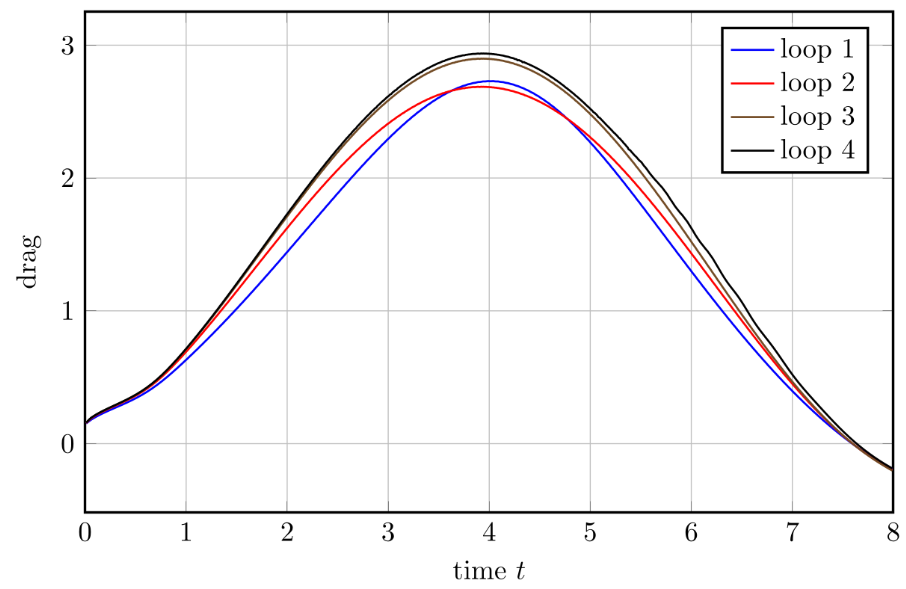
Figure 9: Drag over all DWR loops.
Finally, in Fig. 10 we present the discrete primal solution on the final DWR loop as well as the adaptively refined spatial meshes for all four DWR loops at time point \(t=5\). The spatial refinement remains concentrated close to the cylinder and in the wake, as confirmed by the selected meshes and solution snapshots. The drag and lift histories are smooth and consistent with the benchmark results, which indicates that the adaptive discretization resolves the relevant time dependent features and the Stokes projections avoids spurious oscillations.




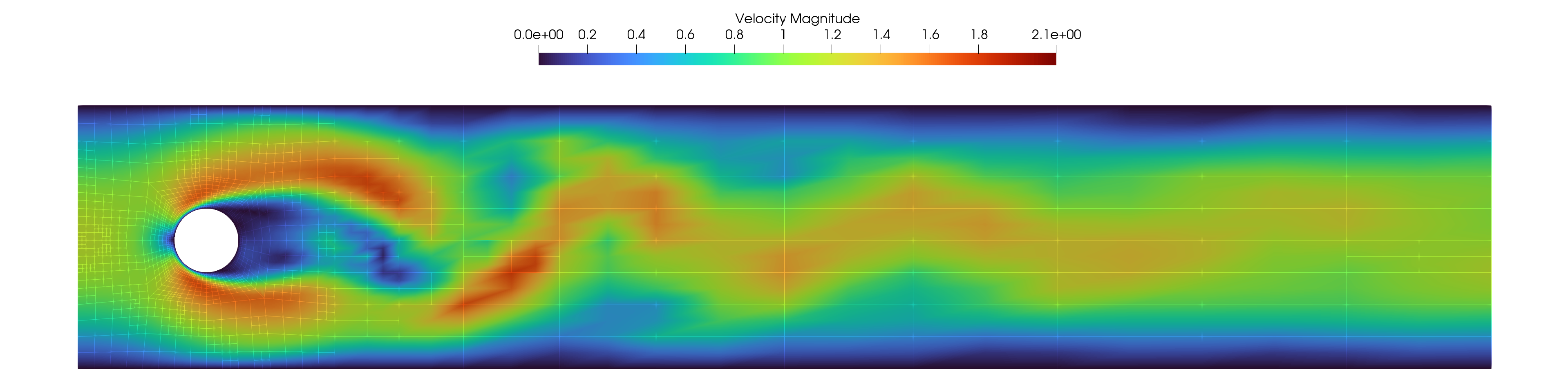
Figure 10: Adaptive refinement history and final-loop solution at \(t=5\). The first four panels show the meshes generated over the adaptive loops. The last two panels show a refined view of the final mesh and the corresponding discrete solution.. a — Adaptive mesh after loop 1., b — Adaptive mesh after loop 2., c — Adaptive mesh after loop 3., d — Adaptive mesh after loop 4., e — Discrete solution on the final loop.
6 Conclusion↩︎
We have developed a goal-oriented space-time adaptive finite element method for the incompressible Navier–Stokes equations based on the Dual Weighted Residual method. The approach combines discontinuous Galerkin time discretization, inf-sup stable mixed finite elements in space, adaptive refinement in space and time, and a slab-wise Newton–Krylov solver with geometric multigrid preconditioning. The numerical results show that this combination yields effective control of the goal quantities on dynamically adapted meshes.
The main computational benefit of the DWR approach is its problem-driven refinement. The estimator identifies those regions in space and time that are most relevant for the chosen output and thereby focuses resolution where it matters for the quantity of interest. At the same time, the results show that this accuracy comes at a substantial cost. In addition to the primal problem, the adaptive loop requires the repeated solution of a dual problem and the evaluation of weighted residual contributions. The efficiency of the overall approach therefore depends not only on the quality of the estimator, but equally on the robustness of the underlying iterative solvers.
The Newton iteration counts are essentially unaffected by the choice of linear preconditioner, whereas the GMRES iteration counts depend strongly on it. Thus, the additional cost of the DWR framework is governed primarily by the linear solver performance for the primal and dual subproblems. In this setting, geometric multigrid provides the required robustness, while ILU does not yield a competitive performance. This is especially important for higher-order discretizations, where the linear systems become more demanding and the dual solve adds a further substantial burden. For goal-oriented space-time adaptivity, robust preconditioning is therefore essential.
Overall, the results show that DWR-based space-time adaptivity is effective for goal-oriented error control, provided that it is paired with scalable linear algebra. The practical cost of the method is determined by the interplay between estimator quality and solver performance. Future work should therefore address both aspects together, in particular through cheaper dual solves, more selective dual updates, and improved multilevel solvers for higher-order and larger-scale space-time discretizations.
Acknowledgement↩︎
Computational resources (HPC cluster HSUper) have been provided by the project hpc.bw, funded by dtec.bw - Digitalization and Technology Research Center of the Bundeswehr. dtec.bw is funded by the European Union - NextGenerationEU.
References↩︎
\(^{,\ddagger}\) Helmut Schmidt University Hamburg, Faculty of Mechanical and Civil Engineering, Chair of Numerical Mathematics, Holstenhofweg 85, 22043 Hamburg, Germany,
bruchhaeuser@hsu-hamburg.de (\(^\ast\)corresponding author), bause@hsu-hamburg.de↩︎University of Magdeburg, Institute for Analysis and Numerics, Universitätsplatz 2, 39104 Magdeburg, Germany, nils.margenberg@ovgu.de.de↩︎