Loss Smoothing for Stable Adaptation Under Distribution Shift
July 01, 2026
Abstract
In settings such as fine-tuning and reinforcement learning, neural networks are often adapted under distribution shift. Standard adaptation methods typically optimize the target objective directly, inducing an abrupt change from the source training objective. This abrupt transition can distort learned representations, including features that may still be useful for the new task. We investigate whether a more gradual transition can improve adaptation. We propose loss smoothing, a simple approach that interpolates between the source and target training objectives at the start of adaptation. This smooth transition helps to preserve useful features from the source distribution while still enabling the model to specialize to the target distribution. Across controlled supervised shifts, pretrained vision adaptation, offline-to-online and online reinforcement learning, and language model fine-tuning, we find that loss smoothing consistently improves performance, suggesting that smoother objective transitions are a broadly useful tool for model adaptation.
1 Introduction↩︎
Modern neural networks are rarely trained once and then left unchanged. A pretrained language model is adapted to instruction-following data [1], [2]; a classifier trained on one task is updated for the next [3], [4]; a policy trained from offline data is fine-tuned through environment interaction [5]–[7]. In each case, adaptation begins from a model that already contains useful features, but then exposes that model to a new input data distribution, a new learning signal, or even a new objective.
The adaptation problem is therefore not simply to optimize the new objective, but to do so while making effective use of the representations already present in the model. This perspective changes the role of stability in adaptation. Stability is often treated as the opposite of adaptation: a model that stays too close to its source solution may fail to fit the new task, but the goal is not simply to move as much as possible. Many shifts contain both task-shared components, such as reusable features, value estimates, behaviors, or representations, and task-inconsistent components that conflict with the new objective. Successful adaptation should preserve the former while modifying the latter. For example, an offline RL policy may contain useful exploratory behavior even when the offline objective is too conservative for online improvement; a pretrained language model may contain broad general-purpose capabilities even when instruction tuning pushes it toward a narrow response distribution. Prior work has observed related brittleness in feature-distorting fine-tuning [8], offline-to-online RL [6], [7], and overtrained language-model fine-tuning [9].
We argue brittle adaptation can arise not only because the target objective is difficult, but because the transition into it is poorly chosen. In standard fine-tuning, once the new phase begins, the source objective is discarded and the model is optimized directly on the target objective. This hard switch can create large, poorly directed updates exactly when the model has the least information about which learned representations should be preserved.
We propose loss smoothing, a simple method for replacing this discontinuous transition with a smoother objective transition. At the start of an adaptation phase, instead of optimizing only the target objective, we optimize a convex interpolation of the source and target objectives. The interpolation coefficient is then annealed until ordinary target training is recovered. Early updates therefore remain close to the source training dynamics, preserving useful features while the model begins to incorporate target-task information. Later updates recover the target objective, allowing the model to specialize to the new task. The motivation is similar to that of continuation methods, curriculum learning, and neural-network smoothing, which also improve optimization by replacing an abrupt problem with a smoother path [10]–[12].
Our method is deliberately general. The source and target phases may differ in their input distributions, their learning signals, or their loss functions. Loss smoothing only requires an estimate of the previous objective under the current parameters, which can be obtained through replay data, stored targets, or direct access to the previous training distribution. This makes it applicable across settings that are usually studied separately: fine-tuning, supervised continual adaptation, and reinforcement learning.
Empirically, we find that smoothing the transition improves adaptation across all of these settings. In controlled supervised shifts, loss smoothing improves both test accuracy and trainability, suggesting that preserving useful structure can make the new task easier to optimize. Additional supervised and pretrained-vision analyses show that smoothing also reduces transient collapse after task switches and improves the retention-adaptation trade-off during adaptation. In offline-to-online reinforcement learning (RL), smoothing provides a middle ground between conservative methods that remain too close to offline pretraining and online-only methods that fail when exploration is difficult. In online RL, smoothing old and new value targets improves performance even on top of algorithms that already contain stabilizing mechanisms. In language model fine-tuning, smoothing the transition from pretraining to instruction tuning reduces overtraining-induced brittleness, showing that catastrophic adaptation can depend on the path into the downstream objective rather than only on the pretrained checkpoint or final loss.
Our contributions are:
We formulate adaptation as a transition between training objectives and identify the hard switch to the target objective as a source of brittle optimization under distribution shift.
We introduce loss smoothing, a lightweight objective interpolation method for adaptation across input, output, and objective-function shifts.
We show that this simple path-based intervention improves adaptation across continual supervised distribution shifts, pretrained vision adaptation, offline-to-online RL, online RL, and LLM fine-tuning.
We provide evidence that preserving reusable features at the start of adaptation can lead to stronger downstream specialization later in training.
2 Related Work↩︎
2.0.0.1 Adaptation under distribution shift.
Fine-tuning from a pretrained model is a standard approach to adaptation, but several lines of work show that the resulting update can be brittle under distribution shift. Fine-tuning can distort pretrained features and hurt out-of-distribution performance [8], and adaptation can depend strongly on which parts of the network are allowed to change [13]–[15]. Warm-starting a neural network is also not always equivalent to training from scratch with a better initialization, because the optimization trajectory itself changes [16]. Our work shares the view that adaptation should preserve useful pretrained structure, but focuses on a complementary intervention: changing the path of intermediate objectives through which optimization moves from the source objective to the target objective.
2.0.0.2 Continual Learning.
Continual learning studies how models adapt across sequences of tasks without catastrophic forgetting [4]. Classical approaches preserve previous knowledge through parameter regularization [3], replay [17], or distillation from an earlier model [18]. Dark experience replay further stores previous model outputs and replays them as targets during later tasks [19], making it especially close to settings where loss smoothing estimates an old objective from stored targets. Recent work has also emphasized transient failures during task changes, including the stability gap [20], and plasticity loss in deep and reinforcement learning [21]–[24]. Rather than treating stability as a permanent constraint, loss smoothing uses the previous objective only as a temporary guide at the beginning of adaptation, then anneals to the target objective. [25] also study smoothing task transition boundaries, but rely on distribution or data specific heuristics rather than a general interpolation of the source and target objectives.
2.0.0.3 Smooth optimization paths.
The idea that optimization can be improved by replacing a hard problem with a sequence of easier or nearby problems appears in continuation methods [10], curriculum learning [11], and neural-network smoothing or mollification [12]. Gradual domain adaptation similarly studies learning through intermediate distributions between a source and target domain [26]. These methods smooth the data, model, or loss landscape, or assume access to intermediate domains. Loss smoothing instead addresses a different situation: the learner already has a source-trained model, and the goal is to avoid a discontinuous switch to a new objective. The intermediate objectives are constructed by interpolating between the source and target training losses, making the method applicable across changes in inputs, learning signals, and objective families.
2.0.0.4 Offline-to-online reinforcement learning.
Offline-to-online RL studies how to initialize an agent from a fixed dataset and then improve it through online interaction. Offline RL methods such as TD3+BC [27], [28] and SPOT [29] regularize policy learning to avoid unsupported actions, while offline-to-online methods decide how much offline data or conservatism should remain during interaction. AWAC uses offline data to accelerate online RL [5], Cal-QL calibrates conservative offline pretraining for efficient online fine-tuning [6], and RLPD mixes offline and online data during online training [30]. Other offline-to-online methods modify the pretraining or fine-tuning procedure itself [7]. These methods address the same source-to-target tension that motivates our work: remaining too close to the offline policy can limit improvement, while switching too abruptly to unconstrained online RL can destabilize learning. Our contribution is orthogonal to these algorithmic choices: we smooth the transition between the offline and online objectives, and in settings where the loss family changes, we also smooth the objective scale.
2.0.0.5 Language model fine-tuning.
Language model fine-tuning also involves an abrupt transition, from broad pretraining distributions to narrower instruction-tuning or preference-tuning datasets. Prior work shows that fine-tuning can reduce general-purpose or out-of-distribution performance [8], and that longer pretraining can make checkpoints harder to fine-tune through catastrophic overtraining and progressive sensitivity [9]. Source-data mixing is also used in instruction tuning and alignment; for example, InstructGPT includes a pretraining-gradient term to reduce capability regressions during RLHF [1]. Recent work further suggests that including pretraining data during fine-tuning [31] and specialized fine-tuning data during pretraining [32] can both improve downstream performance. We use the setting from [9] to test whether the negative effects of overtraining depend not only on the pretraining checkpoint, but also on the transition path between pretraining and fine-tuning.
3 Loss Smoothing↩︎
We consider a model \(f_\theta\) with parameters \(\theta\) trained through a sequence of training phases \(e = 1,2,\ldots\). We view each training phase as inducing a distribution over inputs \(u\) and learning signals \(s\). The input \(u\) is the object on which the model is evaluated, such as an image, prompt, state, transition, or trajectory. The signal \(s\) specifies how the model should update on that input, such as a label, next-token target, reward, return, advantage, or value target. Thus, each phase induces an objective \[J_e(\theta) = \mathbb{E}_{(u, s) \sim \mathcal{D}_e(\theta)} \left[ \ell_e(\theta; u, s) \right].\] Our formulation naturally exposes three different sources of distribution shift. A shift in \(u\) corresponds to a change in the distribution of input being trained on, such as in domain adaptation or an RL policy exploring different parts of the state space. A shift in \(s\) corresponds to a change in the training signal being provided to the model. This can happen when the target distribution changes in fine tuning settings, when the reward signal changes in RL, or even when the target network is updated when bootstrapping in RL. Finally, the last shift corresponds to a change in \(\ell\), i.e. the formulation of the objective. For example, in offline-to-online RL, the loss function in the offline phase is different than the loss function in the online phase.
Adaptation corresponds to moving from a source objective \(J_s\) to a target objective \(J_t\). Standard fine-tuning performs an abrupt switch discarding the source objective once target training begins. Loss smoothing instead replaces this discontinuous switch with a path of intermediate objectives: \[J_{\alpha}(\theta) = (1-\alpha)J_s(\theta) + \alpha J_t(\theta), \qquad \alpha \in [0,1].\] During adaptation, \(\alpha\) is linearly increased over \(\tau\) steps according to a schedule \(\alpha(k) = \min(k/\tau,\,1)\). At the beginning of adaptation, \(\alpha\) is small, so updates remain close to the source training dynamics. As adaptation proceeds, \(\alpha\) increases toward one, eventually recovering ordinary target training.
Our method is flexible in that it makes no assumptions on what the source training phase was or how it relates to the current phase. The shifts we mention can happen independently and even all at once. The intended role of smoothing is to make the beginning of adaptation informative rather than destructive. If part of the model implements structure that is shared between the source and target phases, the source term discourages early updates from immediately overwriting it. If another part of the model is inconsistent with the target phase, the target term can still move it. Loss smoothing therefore acts as a temporary mechanism for separating task-shared components that should be preserved from task-inconsistent components that should be modified.
This interpretation motivates two design choices. First, the previous phase is represented through an estimate of the source objective, such as replay data or stored targets, rather than only through a local penalty on parameters. This keeps the preservation signal tied to the function or prediction induced by the source phase even after the parameters move. Second, the source term is annealed away. If it remains active for the whole target phase, the method becomes closer to ordinary replay and can prevent specialization to the new task. In our experiments, we estimate the previous objective using replay buffers (offline-to-online RL), direct access to the previous data (LLM fine-tuning and DomainNet ViT adaptation), or a single stored batch of past data (continual supervised learning and online reinforcement learning).
In [sec:exp], we will walk through different case studies of how our method can be applied to different instantiations of distribution shifts.
4 Experiments↩︎
| Setting | Source \(\to\) target | Shift instantiated |
|---|---|---|
| Supervised Adaptation | Previous task \(\to\) current task | Permuted inputs isolate a shift in \(u\); shuffled labels isolate a shift in \(s\), with cross-entropy loss fixed. |
| Offline-to-Online RL | Offline \(\to\) online | Transitions, bootstrapped targets, and sometimes the actor objective all change, corresponding to shifts in \(u\), \(s\), and \(\ell\). |
| LLM Fine-tuning | Pretraining \(\to\) instruction tuning | Prompts, sequences, and target tokens narrow, shifting both \(u\) and \(s\) while retaining a next-token loss form. |
| DomainNet ViT | ImageNet \(\to\) DomainNet | The visual domain and labels change, while the ImageNet source objective is retained through replay or smoothing. |
| Online RL | Previous training phase \(\to\) current rollout phase | The policy changes the visited transitions and bootstrapped value targets, creating continual shifts in \(u\) and \(s\). |
4pt
We evaluate loss smoothing across case studies that instantiate different parts of the objective-shift decomposition in 3. In each setting, we identify a source objective \(J_s\), a target objective \(J_t\), and the way the transition changes inputs \(u\), learning signals \(s\), or the loss family \(\ell\). 1 summarizes these instantiations before we give the experimental details for each case study. After these case studies, 5 probes the mechanism more directly and extends the supervised evidence to pretrained vision adaptation.
4.1 Offline-to-Online RL↩︎


Figure 1: Suite-level interquartile mean results for the MuJoCo, AntMaze, and Adroit offline-to-online RL benchmarks, as well as the overall interquartile mean across all environments. Values are mean \(\pm\) 95% confidence interval.. a — MuJoCo results., b — AntMaze results., c — Adroit results., d — Overall results.

Offline-to-online RL is a natural testbed for loss smoothing because adaptation can change both the data distribution and the optimization objective. An agent is first pretrained from a fixed offline dataset, and is then fine-tuned with direct environment interaction. Several prior studies have shown that fine-tuning from offline trained initializations can result in worse performance than training directly from scratch [6], [7]. Policies learned from a fixed dataset can overfit to unsupported actions and suffer from biased value estimates, yet overly conservative offline training can limit improvement once interaction begins. The key challenge is to properly leverage imperfect offline knowledge while enabling efficient online exploration and adaptation without destabilizing performance.
In the notation of 3, \(J_s\) is the offline training objective estimated from the fixed dataset and \(J_t\) is the online fine-tuning objective; the transition can change the sampled transitions \(u\), the bootstrapped targets or rewards \(s\), and, for TD3+BC to TD3, the actor loss \(\ell\).
We evaluate our loss smoothing approach on a variety of standard tasks from D4RL [33]. We instantiate loss smoothing on two existing offline-to-online methods. For the MuJoCo locomotion tasks, the offline phase uses TD3+BC [27] pretraining followed by online TD3 [34] fine-tuning. For the AntMaze and Adroit manipulation tasks, we use SPOT [29] offline training followed by SPOT online training. We apply smoothing to both the actor and the critic. For the TD3/TD3-BC actor objective, since we are smoothing between two different objective functions that can have drastically different scale, we apply smoothing to both the objective and its scale. \[\mathcal{L}_{\pi,\alpha}^{\mathrm{MuJoCo}}(\theta) = (1-\alpha)\mathcal{L}_{\pi}^{\mathrm{TD3+BC}}(\theta) + \alpha c_\alpha \mathcal{L}_{\pi}^{\mathrm{TD3}}(\theta),\] where \(\alpha \in [0,1]\) is the smoothing coefficient. We choose the TD3 actor loss scale by log-space interpolation, \(c_\alpha = \exp\left((1-\alpha)\log c_0 + \alpha \log 1\right),\) where \(c_0\) matches the scale of the online actor loss to the offline TD3+BC regime at the start of online fine-tuning, and \(c_\alpha=1\) recovers raw, unconstrained TD3 at the end. This multiplicative annealing is appropriate when the actor objectives differ by orders of magnitude. For AntMaze and Adroit, loss smoothing interpolates between the SPOT offline objectives (computed with offline data) and SPOT online objectives (computed with online data). We provide further details in 9.1.
We train each agent for 1M offline gradient steps followed by 500k online environment steps, using five seeds per environment. We compare against the offline pretrained policy (Offline), online RL from scratch (Online), abrupt fine-tuning from the pretrained agent (Hard-Switch), and offline-to-online baselines SPOT [29], AWAC [5], Cal-QL [6], and OPT [7]. We standardize the online interaction budget, evaluation protocol, offline datasets, and implementation pipeline across methods; stochastic-policy baselines use stochastic versions of the same TD3-style MLP profiles where the algorithm requires action log-probabilities. We report D4RL normalized scores for individual tasks in ¿tbl:tab:main-results?, and aggregate performance with rliable [35] interquartile means with 95% confidence intervals in 1.
1 shows that loss smoothing performs well across the benchmark rather than specializing to a single regime. It achieves the best overall score, the best suite average on MuJoCo and AntMaze, and remains competitive on the Adroit tasks. The environment-level trends illustrate the source-to-target adaptation trade-off in offline-to-online RL. On AntMaze Medium-Diverse (2, right), online training from scratch receives zero average score, so the offline initialization is essential for exploration. On a task like Random HalfCheetah (2, left), however, conservative baselines that remain close to pretraining inherit limitations of poor offline data. Loss smoothing provides a middle ground: it preserves the useful structure of pretraining early in fine-tuning, but gradually removes the offline constraint as online data becomes available.
4.2 LLM Fine-Tuning↩︎
Our next case study considers the overtrained language model setting of [9]. Their results show that longer pretraining can improve the pretrained model while making the resulting checkpoint harder to adapt, a phenomenon they call catastrophic overtraining. They attribute this degradation to progressive sensitivity: as pretraining continues, the model’s parameters become increasingly sensitive to downstream updates. This is a natural fit for our view of adaptation. Instruction tuning abruptly replaces the broad pretraining distribution with a narrow downstream distribution, and the effect can be most severe for checkpoints whose parameters have become highly sensitive to fine-tuning. \(J_s\) is the pretraining objective and \(J_t\) is the instruction-tuning objective; moving between them narrows both the input sequence distribution \(u\) and the target-token learning signal \(s\).
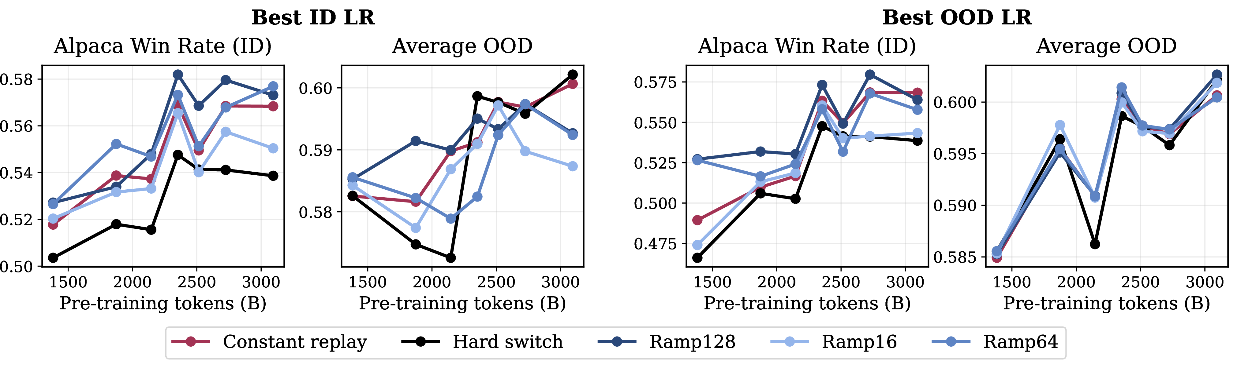
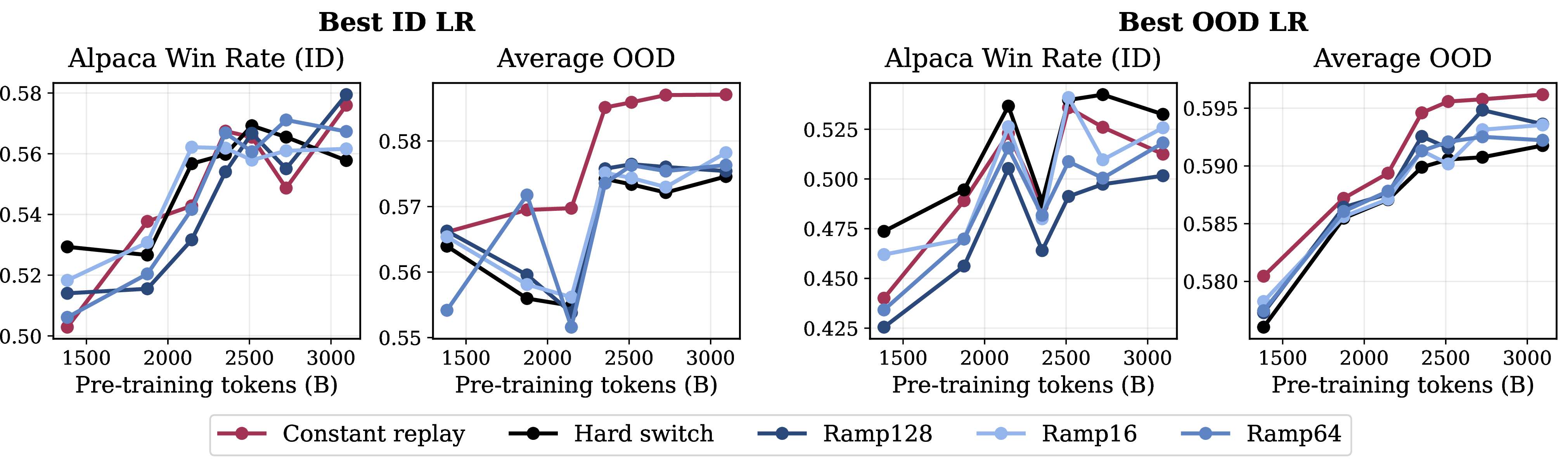
Figure 3: OLMo-1B fine-tuning from checkpoints with different pretraining budgets on Anthropic-HH (top) and Tulu-v1 (bottom). Panels compare hard-switch fine-tuning, loss smoothing, and constant replay under ID-selected and OOD-selected learning rates..
We evaluate whether smoothing this transition reduces the overtraining effect. We fine-tune OLMo-1B [36] checkpoints taken at different pretraining budgets, on two instruction-tuning targets: Anthropic-HH [37] and Tulu-v1 [2]. We compare ordinary fine-tuning (Hard-Switch) to loss smoothing, which gradually anneals from the pretraining loss to the instruction-tuning loss, and to a constant replay baseline that mixes a fixed fraction of pretraining examples throughout fine-tuning. Constant replay is a useful diagnostic because it is an increasingly commonly used method in LLM fine-tuning [31] that also softens the distributional change between pretraining and instruction tuning. For each method, we run three seeds and sweep learning rates in \(\{10^{-5}, 5\cdot10^{-5}, 10^{-4}\}\). See further details in 10.
For each target, we report both in-distribution (ID) instruction-following performance and out-of-distribution (OOD) generalization. ID performance is measured with AlpacaEval win rate [38], while OOD performance is the average over standard evaluation tasks from the language-model evaluation harness [39], including ARC-Challenge, ARC-Easy, HellaSwag, PIQA, and WinoGrande. We sweep learning rates and report two model-selection rules: one that selects the learning rate with the best ID performance, and one that selects the learning rate with the best OOD performance. This separates two practical questions: whether smoothing helps when the practitioner optimizes for the fine-tuning target, and whether it also helps when preserving general capabilities is the primary goal.
3 shows that loss smoothing improves this trade-off, especially in the overtrained regime. When the learning rate is selected for ID performance, loss smoothing and replay retain strong ID performance while showing less degradation from overtraining than hard-switch fine-tuning. When the learning rate is selected for OOD performance, the smoothed variants match or outperform the hard-switch baseline on OOD metrics. The fact that constant replay also improves the transition supports the broader idea that methods that soften the distributional discontinuity between pretraining and instruction tuning reduce overtraining-induced brittleness. Interestingly, while hard-switch performance decreased across pretraining budget, consistent with what was shown in [9], smoothed models maintained or even increased performance, with the single best performance on Tulu-v1 coming from the final, ostensibly most overtrained checkpoint. This suggests that catastrophic overtraining is not solely determined by the pretrained representation or the final instruction-tuning objective, but also by the path used to move between them.
4.3 Online Reinforcement Learning↩︎
Finally, we evaluate loss smoothing in online reinforcement learning settings. RL provides a testbed for evaluating adaptation methods on more natural and complex distribution shifts. Not only does the input data distribution change as the agent learns and explores the environment, but if the agent uses bootstrapping-based methods, then the output distribution also changes as the agent’s value function estimates change over time. Each training phase uses a recent policy-induced distribution over transitions \(u\) and value targets \(s\), rather than an externally specified task boundary. Furthermore, unlike our previous case studies where there were clear boundaries where the training distribution shifted, in RL the shift boundaries themselves are much fuzzier.


Figure 4: Percentage improvements of smoothed agents over baseline agents for TD3 on Brax environments (left) and PPO on DeepMind Control Suite environments (right)..
We evaluate the applicability of our method to both off-policy (TD3 [34]) and on-policy (PPO [40]) algorithms, testing them on two suites of continuous control benchmarks: Brax [41] and DeepMind Control Suite (DMC) [42] implemented in the Mujoco Playground [43], respectively. While we could employ loss smoothing on both the policy and critic losses, we focus on the critic in this section since previous work has shown that critic adaptation can be more difficult than policy adaptation [44]. Furthermore, since our algorithm requires knowledge of task shifts that are not immediately apparent in RL, we simply define a shift as happening every set number of training steps for each task, denoted by a hyperparameter \(n\).
While TD3 already has stabilization mechanisms in the replay buffer and target network, our experience replay buffer is separate and stores the previous outdated targets directly, rather than recomputing the targets based on the current target and policy networks, enabling a more direct interpolation between the old and new objectives. Similarly, with PPO, we save a batch of previous data and corresponding outdated targets to compute the interpolation. We find that for both algorithms, despite the already existing mechanisms to promote network stability, loss smoothing provides significant improvements over the baseline, with some environments seeing nearly double the performance (4). For TD3, we find loss smoothing provides improvements on 5 out of 6 Brax environments, and for PPO, we find that it provides improvements on 15 of the 18 DMC environments that we evaluate on (neither agent made significant progress on the 3 Humanoid environments, excluded from the Figure). Because these results rely on tuning a boundary that is itself difficult to define in online RL, we view them as exploratory evidence that loss smoothing can help in a complex, continuously nonstationary optimization setting. Automatically identifying when such smoothing boundaries should occur is an important challenge that we leave to future work.
5 Smoothing Dynamics↩︎
The preceding experiments show that loss smoothing can improve adaptation, but they do not by themselves identify the mechanism. We therefore analyze these dynamics in three ways. First, we look at which parts of the model move during adaptation, showing that loss smoothing can preserve task-shared features while concentrating updates in task-specific components. Second, we measure the stability gap: the transient collapse in previous-task performance immediately after a task boundary. Finally, we test whether the same retention-adaptation trade-off appears when adapting an ImageNet-pretrained ViT to DomainNet.
5.1 Continual Supervised Learning↩︎

We now consider synthetic supervised adaptation setups with controlled data distribution shifts. We base our experiments on CIFAR-10 [45] and use two standard transformations [46]: permuted input and shuffled labels. Although these are simplified settings, they allow us to cleanly isolate the effects of distribution shifts in just the inputs or outputs, and to easily compare the internal changes in the model during training.
In the notation of 3, adjacent tasks define the source and target objectives; permuted inputs isolate a change in \(u\), while shuffled labels isolate a change in the learning signal \(s\). In the permuted-input setting, a randomly generated permutation in the input space, \(P_k^{x} : \mathcal{X} \rightarrow \mathcal{X}\), reorders pixel locations. Task \(k\) is defined by the transformed dataset \(\mathcal{D}_k = \left\{ \left(P_k^{x}(x_i), y_i\right) \right\}_{i=1}^n\). In the shuffled-label setting, a randomly generated permutation in the output space, \(P_k^{y} : \mathcal{Y} \rightarrow \mathcal{Y}\), remaps the labels, and task \(k\) is defined as \(\mathcal{D}_k = \left\{ \left(x_i, P_k^{y}(y_i)\right) \right\}_{i=1}^n\). In both settings, after the task switch, the model is only trying to learn the new task, and not preserve performance on the previous task. Each seed is run on a sequence of 100 independently generated tasks, and we show the average performance with standard deviation.
In Figure 5, we compare loss smoothing to a baseline, both with optimal hyperparameters. Loss smoothing outperforms the baseline on the test set, with larger gains on later tasks. Interestingly, training accuracy is also higher, suggesting that the improvement stems from better trainability, despite the additional regularization to the previous task.
Main components To demonstrate the importance of the two main design choices of our method—how regularization is applied (via loss smoothing) and when it is applied (only at the beginning of training on each task)—we add two additional baselines in Figure 5. First, we compare to an EWC [3] variant of our method, which follows the same training procedure and regularization coefficient schedule but changes the regularization term from the loss on the replay data to EWC regularization. In principle, EWC should also encourage preservation of task-shared weights while allowing task-inconsistent weights to change. However, it is substantially less effective in our experiments. We hypothesize that this is due to the local nature of EWC, which makes it ineffective after the first few steps. Second, we compare with a variant of our method with a long decay schedule, where the number of loss smoothing steps \(\tau\) is equal to the whole length of training, making it closer to standard replay methods from continual learning [17]. The long decay schedule leads to a significant performance degradation in both setups. We attribute this to excessive emphasis on old data, which prevents the model from effectively adapting to the new task.

Method analysis To validate our initial motivation that loss smoothing facilitates adaptation by helping the model identify which components to preserve and which to modify, in Figure 6 we analyze the drift in network activations from the final checkpoint of Task 0 as the model is trained on subsequent tasks. To compare two models, we take a random subset of examples and compute layer-wise activations for each model via a forward pass. For each layer, we then compute the average cosine similarity between the corresponding activations. In the permuted-input setting, we apply the permutation associated with the model checkpoint’s task to the inputs before the forward pass.
In the permuted-input setting, the functions implemented by all layers except the first one can, in principle, be shared across tasks, whereas the first layer cannot due to the different pixel orderings. We observe that the first-layer activations change substantially less under loss smoothing than under the baseline, while the final predictions change to a similar extent for both methods. This suggests that loss smoothing preserves the functions of the deeper layers by primarily adapting the first layer to reproduce the appropriate activations under the new input permutation.
In the shuffled-label setting, all layers except the last one can be shared across tasks, since only the image-label correspondence changes. Here, the penultimate-layer activations change much less with loss smoothing than with the baseline, while the final predictions again change similarly for both methods. This indicates that loss smoothing preserves the shared representation and primarily adapts the last layer, whereas the baseline modifies the network more uniformly.
Additionally, we observe that EWC is ineffective at redistributing changes across the model, while loss smoothing with a long decay schedule alters the final predictions too strongly and prevents the model from learning an appropriate solution for the current task. In Appendix 7.2, we further show that the positive effect of loss smoothing cannot be explained by implicit learning rate warm-up or increased data per optimization step, and provide additional ablations of hyperparameter effects.
5.2 Stability gap↩︎
Beyond final performance, abrupt task switches can also create a stability gap: a transient drop in performance on previous tasks immediately after the learner begins training on a new task [20], [47]. This is distinct from final forgetting. A model may eventually recover some previous-task performance, but the first updates after a distribution shift can still temporarily destroy useful behavior.
We evaluate this effect on Split-CIFAR-10, where the ten CIFAR-10 classes are partitioned into a sequence of five two-class tasks and the model is trained on the tasks sequentially. This setting creates sharp class-distribution changes at known task boundaries while preserving a shared visual input space, making it a direct test of whether the optimizer can incorporate the new classes without temporarily disrupting features that remain useful for earlier classes. We track previous-task accuracy throughout training, with particular attention to the updates immediately after each task switch. As shown in 7, loss smoothing substantially reduces the transient performance drop compared to the hard-switch baseline.

To apply loss smoothing in this setting, we use a per-sample replay weight. Let \(\rho\) denote the target replay weight. When an example from the current task is added to the replay buffer, we anneal its weight from \(1-\rho\) to \(\rho\) rather than changing its contribution abruptly. Conversely, when training begins on a new task, examples from the new task are annealed from weight \(0\) to \(1-\rho\). Thus, for an example \(z_i\) with task-boundary time \(t_i\), we use a ramp \(a_i(t)=\min((t-t_i)/\tau,1)\) and set \[\begin{align} w_i^{\mathrm{new}}(t) &= a_i(t)(1-\rho),\\ w_i^{\mathrm{replay}}(t) &= (1-a_i(t))(1-\rho)+a_i(t)\rho. \end{align}\] This per-sample form is the same idea as the global objective interpolation in 3, but applied at the granularity of replay membership. It shows that loss smoothing is not only a way to improve final adaptation, but also a way to control the transient optimization path at the moment a distribution shift occurs.
The reduced stability gap also supports the feature-preservation view of loss smoothing. If a hard switch forces early updates to rapidly reorganize internal representations, previous-task accuracy can collapse even before final forgetting is measured. By reducing this transient collapse, loss smoothing suggests that useful features are preserved not only at the final checkpoint, but throughout the optimization trajectory while the model moves from one task objective to the next. The DomainNet experiment below asks whether this improved path also changes the final adaptation-retention frontier in a larger pretrained vision model.
5.3 Vision Transformer DomainNet Adaptation↩︎

We next test whether the same preservation-adaptation dynamics persist in a larger pretrained vision model. Starting from an ImageNet-pretrained ViT, we adapt to each DomainNet domain separately and measure the trade-off between in-domain DomainNet accuracy and retention of the original ImageNet classifier. In the notation of 3, ImageNet classification defines the source objective and single-source DomainNet training defines the target objective; further experimental details are in 8. This complements the stability-gap analysis: there we measured transient retention along the path, while here we compare the final retention-adaptation frontier induced by different paths.
8 shows that both constant ImageNet replay and loss smoothing improve over the hard switch, which rapidly loses ImageNet performance. This supports the central claim that information from the previous objective remains useful during adaptation: preserving the source task does not merely protect ImageNet accuracy, but also slightly improves in-domain DomainNet accuracy relative to abrupt fine-tuning.
The comparison between loss smoothing and matched-duration replay isolates the role of the path to the target objective. When the ImageNet objective is used for the same fraction of training, loss smoothing achieves better DomainNet adaptation than replay, indicating that annealing the source objective away is more effective than keeping a fixed replay weight and then abruptly removing it. The duration sweep also shows that the source objective need not remain active for all of training: using it for only 5, 10, or 25% of training already recovers much of the ImageNet retention lost by the hard switch, while longer smoothing horizons continue to improve the retention-adaptation frontier.
6 Discussion↩︎
Across supervised task shifts, pretrained vision adaptation, offline-to-online RL, online RL, and LLM fine-tuning, we find that abrupt changes in the input distribution \(u\), learning signal \(s\), or loss family \(\ell\) can make the updates after the shift brittle. Loss smoothing reduces this brittleness by keeping early updates partially tied to the source objective while the model begins to incorporate target-task information.
The case studies in our work show that the source objective often contains useful structure. Supervised replay preserves reusable features, offline RL pretraining can provide behaviors and value estimates that help early online learning, and language-model pretraining supports broad capabilities that can be damaged by narrow instruction tuning. Loss smoothing keeps these sources of structure active at the start of adaptation, then anneals them away so that the model can specialize.
6.0.0.1 Limitations
The method requires access to, or an estimate of, the source objective, which may involve replay data, stored targets, or continued access to previous training data. It also introduces schedule choices, and the right smoothing boundary is especially unclear in online RL, where the data distribution changes continuously with the policy. When loss families have very different units, as in TD3+BC-to-TD3 fine-tuning, their scales must also be handled carefully. Compared to normal training, loss smoothing also requires more compute at the start of adaptation. Finally, our ablations show that smoothing for too long can hurt by keeping the learner tied to outdated data. Automatically detecting when to smooth, how long to smooth, and how to normalize incompatible objectives are important directions for future work.
Acknowledgments↩︎
We would like to thank Andrei Mircea for the valuable comments and discussions. We also thank Mila (mila.quebec) and its IDT team for providing and supporting the computing resources used in this work. Ekaterina Lobacheva is supported by IVADO and the Canada First Research Excellence Fund. Sarath Chandar is supported by the Canada CIFAR AI Chairs program, the Canada Research Chair in Lifelong Machine Learning, and the NSERC Discovery Grant.
7 Continual Supervised Learning↩︎
7.1 Experimental Details↩︎
We use a simple 3-layer MLP: input layer (3072 → 100) → ReLU → hidden layer (100 → 100) → ReLU → output layer (100 → 10). The model is trained with SGD, batch size 256, for 20k steps per task. We run all experiments with 10 different random seeds and show average results with standard deviation in all the plots.
We ran baseline, loss smoothing, and EWC experiments across several learning rates and weight decay values, and found that a learning rate of 0.01 and weight decay of 0.001 were optimal for all methods. These values are used in all experiments. For loss smoothing, we additionally search for the optimal number of smoothing steps from \([100, 500, 1000, 5000, 10000, 20000]\), finding it to be 500 for permuted input and 5000 for shuffled labels. A similar search for EWC yields optimal regularization steps of 500 for permuted input and 100 for shuffled labels.
7.2 Ablations↩︎

The positive effect of loss smoothing could potentially arise from using a learning rate warm-up at the start of each task or from having more data per optimization step. In Figure 9, we compare to the baseline with these modifications. For the baseline with learning rate warm-up, we use the same schedule for the current-batch loss coefficient as in loss smoothing, but set the replay term to zero. Warm-up helps in the permuted-input setting, achieving results comparable to loss smoothing, but has little effect for shuffled labels. For the baseline with more data, we double the batch size to match the data size used per optimization step in loss smoothing. While this slightly improves optimization, it does not replicate the benefits of loss smoothing.


In Figures 10 and 11, we analyze the effects of two main hyperparameters of loss smoothing: the number of smoothing steps \(\tau\) and the amount of replay data. For the number of steps, there exists an optimal value that depends on the task (here, 500 for permuted input and 5000 for shuffled labels). Fewer steps reduce the positive effect of loss smoothing, while too many steps degrade performance by overemphasizing older data. For the amount of replay data, a batch of 256 examples is generally sufficient. Using fewer examples can hurt performance, while using more does not provide additional benefits.
8 DomainNet Experimental Details↩︎
We run the full-DomainNet ViT experiments with a vit_base_patch16_224 model initialized from ImageNet pretraining. We keep the pretrained 1000-way ImageNet head, remove the classifier from the shared backbone, and add a randomly initialized
345-way DomainNet head. Thus, adaptation changes the shared representation and DomainNet head, while ImageNet retention is measured with the preserved ImageNet head.
We use all six DomainNet domains: clipart, infograph, painting, quickdraw, real, and sketch. For the single-source runs in 8, each run trains on one source domain and evaluates in-domain accuracy on that same domain’s official test split. We construct a stratified 10% validation split from the official training split for model selection and leave the official test split unchanged. All images are resized and cropped to \(224\times224\) using ImageNet normalization.
All methods are trained for 60 epochs with batch size 256, AdamW, learning rate \(2\times10^{-5}\), weight decay \(0.1\), 5% linear learning-rate warmup, and cosine decay. The hard-switch baseline minimizes only the DomainNet cross-entropy loss after adaptation begins. Replay and loss smoothing additionally use ImageNet training batches through the original ImageNet head. Let \(\lambda_t\) be the ImageNet loss coefficient at step \(t\); the optimized loss is \[(1-\lambda_t)\mathcal{L}_{\mathrm{DomainNet}} + \lambda_t\mathcal{L}_{\mathrm{ImageNet}} .\] Replay uses a constant \(\lambda_t=0.5\) throughout training. Loss smoothing starts with \(\lambda_0=1\) and linearly anneals to \(0\) over a specified fraction of training: 5, 10, 25, 50, 75, or 100%. We also run matched-duration replay controls, where \(\lambda_t=0.5\) is held constant for the same initial fraction of training and then set to \(0\).
We summarize final epoch-60 checkpoints. For each method, we form a \(3\times6\) score matrix from three seeds and six source domains. We report the interquartile mean (IQM) with 95% percentile bootstrap confidence intervals using 50,000 bootstrap samples. The bootstrap resamples seeds while keeping the six source domains as the task strata.
| Method | DomainNet ID | ImageNet retention |
|---|---|---|
| Hard switch | 75.93 [75.84, 76.04] | 14.01 [12.77, 15.35] |
| Replay, 100% | 76.22 [76.18, 76.29] | 83.90 [83.78, 84.00] |
| Replay, 5% | 76.09 [76.03, 76.14] | 51.50 [50.41, 52.75] |
| Replay, 10% | 76.02 [75.95, 76.09] | 68.18 [67.57, 68.62] |
| Replay, 25% | 76.06 [76.01, 76.11] | 79.01 [78.81, 79.20] |
| Replay, 50% | 76.09 [76.05, 76.15] | 82.53 [82.40, 82.66] |
| Replay, 75% | 76.16 [76.11, 76.21] | 83.60 [83.50, 83.70] |
| Loss smoothing, 5% | 76.13 [76.07, 76.17] | 50.33 [49.74, 51.02] |
| Loss smoothing, 10% | 76.20 [76.14, 76.27] | 68.28 [67.80, 68.57] |
| Loss smoothing, 25% | 76.23 [76.15, 76.32] | 78.84 [78.74, 78.94] |
| Loss smoothing, 50% | 76.34 [76.26, 76.40] | 82.45 [82.29, 82.61] |
| Loss smoothing, 75% | 76.40 [76.34, 76.46] | 83.43 [83.28, 83.58] |
| Loss smoothing, 100% | 76.42 [76.38, 76.48] | 83.86 [83.75, 83.98] |
9 Offline-to-Online RL↩︎
9.1 Experimental Details↩︎
For the offline-to-online RL case study, offline-initialized methods use 1M offline gradient steps followed by 500k online environment steps, with five random seeds per environment. Our MuJoCo loss-smoothing instantiation uses a TD3+BC-style offline objective [27] and TD3 online fine-tuning [34]. Our AntMaze and Adroit loss-smoothing instantiation uses SPOT-style offline training and SPOT online fine-tuning [29].
9.1.0.1 Tasks and budgets.
We use the D4RL benchmark suite [33] with the following dataset identifiers: halfcheetah-medium-v2,
hopper-medium-v2, walker2d-medium-v2, halfcheetah-random-v2, hopper-random-v2, and walker2d-random-v2 for MuJoCo locomotion; antmaze-umaze-v2,
antmaze-umaze-diverse-v2, antmaze-medium-play-v2, and antmaze-medium-diverse-v2 for AntMaze; and pen-cloned-v1, hammer-cloned-v1, door-cloned-v1, and
relocate-cloned-v1 for Adroit. Unless otherwise noted, results use seeds \(0,\ldots,4\). Offline-initialized methods use 1M offline gradient updates followed by 500k online environment steps. The
online-from-scratch control uses the same 500k online-step budget with no offline pretraining, and the offline control evaluates the pretrained checkpoint without online updates.
9.1.0.2 Replay and online updates.
All online training runs use a single training environment and one gradient update per environment step. Evaluation is vectorized, but training is not. Mini-batches have size 256. For smoothed TD3+BC-to-TD3 runs, each update draws one batch from the online replay buffer and one independent batch from the fixed D4RL dataset; the offline actor/critic losses are computed on the offline batch, the online actor/critic losses are computed on the online batch, and the losses are interpolated after they are computed. The hard-switch and online TD3 controls do not use the offline loss branch. TD3-family online replay buffers have capacity 2M transitions. For SPOT-family support tasks, non-smoothed SPOT fine-tuning follows the SPOT replay convention by initializing a mixed replay buffer with offline transitions and then appending online data. Smoothed SPOT uses a separate online-only replay buffer for the online branch and samples the offline branch directly from the D4RL data; the mixed and online SPOT buffers each have capacity 2M. AWAC [5] uses a uniform replay buffer initialized with the offline data and appended online data. Cal-QL [6] uses separate 2M-transition offline and online replay buffers and, after online data is available, samples half of each update batch from each buffer. OPT [7] uses uniform replay in our implementation: the first 25k online steps are collected with the frozen offline policy, then the online critic is adapted for 50k critic-only updates, and then fine-tuning proceeds within the same 500k online interaction budget. We do not use the prioritized replay variant of OPT.
9.1.0.3 Evaluation and aggregation.
We evaluate every 10k online environment steps, for 50 evaluations over the 500k-step budget. MuJoCo evaluation uses 128 episodes; AntMaze and Adroit use 10 episodes. Evaluation returns are computed with the unmodified environment rewards and are
converted to D4RL normalized scores using the standard get_normalized_score convention. Final-return tables average the last three evaluation points within each seed and report mean \(\pm\) standard error
across seeds for each environment. Suite-average rows are arithmetic averages over the environment-level means in the suite, with standard errors computed across environments. Learning-curve bands are standard errors across seeds. The suite-level IQM plots
use rliable [35] with 95% bootstrap confidence intervals.
9.1.0.4 Architectures and optimization.
Within each algorithm family, all variants share the same network and optimizer profile. Dense MuJoCo TD3+BC, TD3, and TD3+OPT runs use two-layer 256-unit ReLU actor and critic MLPs with layer normalization and deterministic tanh-scaled actions. AntMaze SPOT runs use the same two-layer ReLU MLP without layer normalization. Adroit SPOT runs use the two-layer ReLU MLP with post-activation layer normalization and OPT-style small uniform final-layer initialization. AWAC and Cal-QL use stochastic versions of these TD3-style profiles: the actor head is replaced with a tanh-squashed Gaussian distribution head so that the algorithms can evaluate action log-probabilities, while the actor and critic torsos keep the same two-layer 256-unit ReLU architecture and domain-specific layer-normalization choices as the corresponding TD3/SPOT runs. The main optimization hyperparameters are summarized in 3.
| Component | Values |
|---|---|
| TD3-family online training | Actor learning rate \(10^{-4}\); critic learning rate \(3\cdot10^{-4}\); discount \(\gamma=0.99\); target-update rate \(\tau=0.005\); exploration noise \(0.1\); target policy noise \(0.2\); target-noise clip \(0.5\); delayed actor/target updates every two critic updates. |
| TD3+BC offline pretraining | 1M gradient updates; bc_alpha=2.5. |
| SPOT support model and critic/actor updates | Actor learning rate \(10^{-4}\); critic learning rate \(3\cdot10^{-4}\); the same TD3 target and exploration parameters; VAE learning rate \(10^{-3}\); VAE hidden dimension 750; 100k VAE updates; \(\beta=0.5\); one VAE sample for the support cost. |
| SPOT support coefficient | \(\lambda_t=\lambda_0\max(\lambda_{\mathrm{floor}},1-t/10^6)\), with \((\lambda_0,\lambda_{\mathrm{floor}})=(0.05,0.2)\) for AntMaze and \((1.0,0.5)\) for Adroit. The SPOT baseline uses this cooling schedule; the hard-switch support baseline disables it. |
| AWAC | Actor and critic learning rates \(3\cdot10^{-4}\); advantage temperature \(\lambda=0.1\) on AntMaze and \(1.0\) otherwise; exponentiated advantages clipped at 100. |
| Cal-QL | Actor learning rate \(10^{-4}\); critic and entropy-temperature learning rates \(3\cdot10^{-4}\); CQL coefficient 5; 10 sampled actions; CQL temperature 1; offline calibration. On AntMaze we use the reference sparse-reward settings: training reward transform \(10r-5\), Lagrange CQL with target action gap 0.8, max target backup, and CQL-difference lower clipping at \(-200\). |
| OPT | Uniform replay; 25k online collection steps with the frozen offline policy; 50k critic-only online-critic adaptation updates; OPT inner critic learning rate \(3\cdot10^{-4}\). The mixed-Q actor schedule uses \(\kappa=1\) for random MuJoCo, \(0.3\to0.9\) over 150k steps for medium MuJoCo, \(0.1\to0.9\) over 100k steps for AntMaze, and \(0.1\to0.9\) over 250k steps for Adroit. |
4pt
9.1.0.5 Reward transforms.
Reward transforms are applied only for training, taken from reference implementations; evaluation always uses raw environment rewards before D4RL normalization. SPOT-family AntMaze runs, including loss smoothing and SPOT+OPT, use the SPOT reward transform \(r'=r-1\). AWAC uses \(r'=r-1\) on AntMaze and raw rewards elsewhere. Cal-QL uses \(r'=10r-5\) on AntMaze and raw rewards elsewhere. The raw TD3 online-from-scratch control on AntMaze also uses \(r'=10r-5\).
9.1.0.6 Loss-smoothing schedule.
Loss smoothing uses an environment-step clock. Let \(h\) be the smoothing horizon and \(\alpha_t=\min(t/h,1)\). The offline weight is \(1-\alpha_t\), the online weight is \(\alpha_t\), and both actor and critic losses are smoothed: \[\mathcal{L}_t = (1-\alpha_t)\mathcal{L}_{\mathrm{offline}} + \alpha_t \mathcal{L}_{\mathrm{online}} .\] For the main results, dense MuJoCo and Adroit cloned tasks use a 50k-step ramp, while AntMaze uses a 250k-step ramp. We also run ramp-length ablations at 10k, 50k, 100k, and 250k steps, with the main-result plots selecting one ramp per domain. For MuJoCo TD3+BC-to-TD3 actor smoothing, the online TD3 actor branch is normalized by a stop-gradient \(\mathbb{E}[|Q|]\) scale and multiplied by a log-space scale annealing factor, \[c_t = \exp\left((1-\alpha_t)\log c_0 + \alpha_t\log c_1\right),\] where \(c_0\) is the offline TD3+BC behavior-cloning coefficient read from the checkpoint and \(c_1\) is the current online TD3 \(|Q|\) scale. This preserves a smooth handoff between the TD3+BC actor-loss units and the online TD3 actor-loss units. Equivalently, if the online actor loss is written in raw TD3 units, this endpoint corresponds to scale one. The SPOT-to-TD3 ablation uses analogous log-space scale annealing when the online branch is changed from the SPOT actor objective to the unconstrained TD3 actor objective.
9.2 Additional Results and Ablations↩︎
3.2pt
@lccccccc@ Env. & Offline & Online & Hard-Switch & AWAC & Cal-QL & OPT &
HalfCheetah-M & 47.3\(\pm\)0.0 & 29.5\(\pm\)7.5 & 48.2\(\pm\)0.3 & & & 48.5\(\pm\)0.2 & 48.2\(\pm\)0.5
Hopper-M & 47.2\(\pm\)1.9 & 69.6\(\pm\)18.6 & & 81.9\(\pm\)4.1 & 74.4\(\pm\)5.6 & & 99.9\(\pm\)5.5
Walker2d-M & 83.2\(\pm\)0.4 & 61.5\(\pm\)13.9 & & 86.4\(\pm\)0.2 & 87.4\(\pm\)0.4 & 94.6\(\pm\)1.1 &
HalfCheetah-R & 8.3\(\pm\)0.3 & 18.4\(\pm\)0.6 & & 32.9\(\pm\)0.6 & 13.1\(\pm\)1.8 & 37.5\(\pm\)1.0 &
Hopper-R & 13.5\(\pm\)7.1 & & 55.0\(\pm\)9.8 & 18.1\(\pm\)1.3 & 11.9\(\pm\)2.0 & 14.9\(\pm\)2.1 &
Walker2d-R & 7.2\(\pm\)3.4 & & & 4.2\(\pm\)0.3 & 11.0\(\pm\)3.8 & 9.0\(\pm\)1.7 & 68.0\(\pm\)13.1
Average & 34.5\(\pm\)12.3 & 53.2\(\pm\)9.5 & & 45.9\(\pm\)13.7 & 42.0\(\pm\)14.1 & 51.7\(\pm\)16.5 &
UMaze & 26.0\(\pm\)16.0 & 0.0\(\pm\)0.0 & 40.7\(\pm\)14.2 & 6.7\(\pm\)1.5 & & 44.0\(\pm\)21.9 &
UMaze-Div & 18.0\(\pm\)9.7 & 0.0\(\pm\)0.0 & 67.7\(\pm\)10.6 & 14.7\(\pm\)6.2 & 47.3\(\pm\)3.9 & &
Medium-Play & 58.0\(\pm\)7.3 & 0.0\(\pm\)0.0 & 55.7\(\pm\)7.4 & 0.0\(\pm\)0.0 & 0.0\(\pm\)0.0 & &
Medium-Div & 38.0\(\pm\)11.1 & 0.0\(\pm\)0.0 & 21.7\(\pm\)7.1 & 0.0\(\pm\)0.0 & 28.0\(\pm\)16.7 & &
Average & 35.0\(\pm\)8.7 & 0.0\(\pm\)0.0 & 46.4\(\pm\)9.9 & 5.3\(\pm\)3.5 & 43.5\(\pm\)20.8 & &
Pen & 47.8\(\pm\)9.0 & 101.6\(\pm\)8.8 & 114.9\(\pm\)4.0 & 55.3\(\pm\)4.7 & 103.0\(\pm\)7.1 & &
Hammer & 2.2\(\pm\)0.4 & 100.5\(\pm\)11.6 & 117.3\(\pm\)1.4 & 0.3\(\pm\)0.0 & & 112.9\(\pm\)5.8 &
Door & 0.3\(\pm\)0.2 & 58.3\(\pm\)14.2 & 0.3\(\pm\)0.2 & -0.1\(\pm\)0.0 & 19.9\(\pm\)14.6 & &
Relocate & & -0.1\(\pm\)0.0 & -0.1\(\pm\)0.0 & -0.2\(\pm\)0.0 & -0.2\(\pm\)0.0 & & -0.1\(\pm\)0.0
Average & 12.6\(\pm\)11.8 & 65.1\(\pm\)23.9 & 58.1\(\pm\)33.5 & 13.8\(\pm\)13.8 & 60.9\(\pm\)30.0 & &
Overall & 27.3 & 39.4 & 58.2 & 21.7 & 48.8 & &
We provide additional learning curves in 12. In dense MuJoCo tasks, loss smoothing typically retains the fast improvement of offline initialization while allowing the policy to move beyond the constraints of the offline objective. In the support-constrained AntMaze and Adroit tasks, the curves show the complementary role of the offline objective: early smoothing stabilizes fine-tuning in regimes where online data alone can be difficult to use.

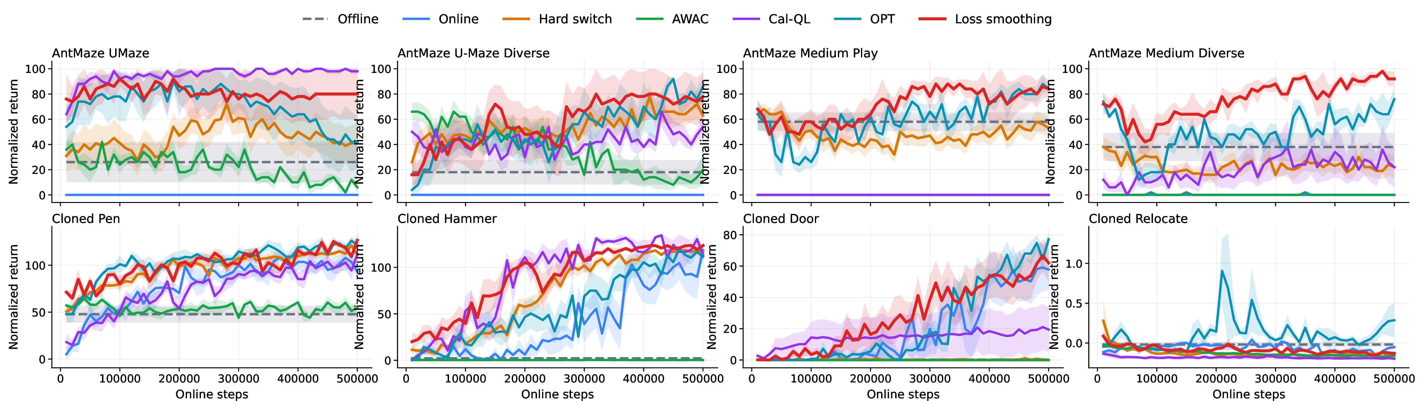
Figure 12: Additional offline-to-online RL learning curves. Shaded regions denote standard error across seeds. These curves complement the selected examples in 2 by showing the broader suite-level behavior across dense locomotion and support-constrained environments.. a — Dense MuJoCo locomotion tasks., b — AntMaze and Adroit tasks.
We also ablate the number of environment steps over which the source objective is annealed away. 13 shows that the preferred horizon depends on the domain. MuJoCo and Adroit benefit from a shorter handoff, where online interaction quickly provides useful target-task information. AntMaze benefits from a longer handoff, consistent with the sparse-reward setting where the offline policy remains important for exploration over a larger fraction of fine-tuning. These results support treating the smoothing horizon as a domain hyperparameter rather than a fixed constant.


Figure 13: Offline-to-online RL ablations for the loss-smoothing horizon. Each panel reports the suite-level interquartile mean with 95% bootstrap confidence intervals. The main results use a domain-specific horizon selected from these ablations: 50k environment steps for MuJoCo and Adroit, and 250k environment steps for AntMaze.. a — MuJoCo., b — AntMaze., c — Adroit.
10 Overtrained LLM Fine-tuning↩︎
10.0.0.1 OLMo-1B checkpoints.
We follow the OLMo-1B setting from [9]. All runs initialize from public
allenai/OLMo-1B-hf checkpoints [36] and use the corresponding OLMo tokenizer. We
fine-tune all model parameters; no layers are frozen and no adapter modules are introduced. The checkpoint grid is shown in 4. We use the token counts in the checkpoint names as the pretraining budget.
| Checkpoint | Short name | Pretraining tokens |
|---|---|---|
| step330000-tokens1383B | 1383B | 1.383T |
| step447000-tokens1874B | 1874B | 1.874T |
| step512000-tokens2146B | 2146B | 2.146T |
| step561250-tokens2353B | 2353B | 2.353T |
| step600000-tokens2515B | 2515B | 2.515T |
| step650000-tokens2725B | 2725B | 2.725T |
| step738000-tokens3094B | 3094B | 3.094T |
10.0.0.2 Instruction-tuning data.
We use two target distributions. For Anthropic-HH, we use the Anthropic/hh-rlhf training split [37] and keep the chosen transcript from each preference pair. Each transcript is parsed into alternating user and assistant turns, and each turn is serialized as
role: content
with blank lines between turns. For Tulu-v1, we use a deterministic 200k-example subset of the allenai/tulu-v1-sft-mixture training split [2], selected by shuffling with seed 0 and taking the first 200k examples. We serialize each message as role: content, separated by blank lines. The resulting tokenized caches contain 160,800 Anthropic-HH
examples and 200,000 Tulu-v1 examples. Training sequences are packed to length 1024. We do not use a validation split or early stopping during fine-tuning.
10.0.0.3 Loss schedules and baselines.
Let \(\mathcal{L}_{\mathrm{pre}}\) denote the next-token loss on replayed pretraining data and \(\mathcal{L}_{\mathrm{inst}}\) denote the next-token loss on the instruction-tuning target. Loss smoothing uses \[\mathcal{L}_t(\theta) = (1-\alpha_t)\mathcal{L}_{\mathrm{pre}}(\theta) + \alpha_t \mathcal{L}_{\mathrm{inst}}(\theta), \qquad \alpha_t = \min(t/\tau, 1).\] We compare three method families. Hard-Switch sets \(\alpha_t=1\) for every fine-tuning step. Loss Smoothing linearly ramps \(\alpha_t\) from 0 to 1 over \(\tau \in \{16,64,128\}\) update steps. Constant Replay is a diagnostic baseline with fixed weights \(0.5\mathcal{L}_{\mathrm{pre}} + 0.5\mathcal{L}_{\mathrm{inst}}\) throughout fine-tuning. The replay data is a 500M-token cap of the top OLMo pretraining components: Common Crawl, Falcon, StarCoder, C4, Reddit, and peS2o, mixed in proportion to their OLMo pretraining weights. Replay is included because it also softens the pretraining-to-instruction distribution shift, but it is not the proposed method.
10.0.0.4 Optimization.
All OLMo-1B fine-tuning runs use AdamW [48] with \(\beta_1=0.9\), \(\beta_2=0.95\), \(\epsilon=10^{-8}\), global gradient clipping at norm 1.0, and weight decay 0. The learning-rate schedule is cosine decay to zero with 20 warmup steps. We use bfloat16 compute with float32 parameters, global batch size 256 packed sequences, sequence length 1024, and per-device parallelism 8. The resulting training lengths are 141 update steps for Anthropic-HH and 483 update steps for Tulu-v1, corresponding to 36.96M and 126.62M target tokens respectively. The learning-rate sweep is \[\eta \in \{10^{-5}, 5\cdot 10^{-5}, 10^{-4}\}.\] For each checkpoint, target, method configuration, and learning rate, we run data-order seeds \(\{0,1,2\}\). This gives \(7\) checkpoints \(\times\) \(2\) targets \(\times\) \(3\) learning rates \(\times\) \(3\) seeds \(\times\) \((1\;\text{hard-switch} + 1\;\text{replay} + 3\;\text{smoothing horizons}) = 630\) OLMo-1B fine-tuning runs.
10.0.0.5 ID evaluation.
ID performance is an AlpacaEval-style pairwise win rate [38]. We generate responses to the 805 prompts from the tatsu-lab/alpaca_eval
eval split with the prompt template
user: <instruction>\n\nassistant:.
Generation uses vLLM [49], bfloat16 weights, temperature 0, top-\(p=1\), maximum 1024 new tokens, minimum 1 new token, and seed 0. We judge each candidate against a target-matched hard-switch reference trained from the 1874B checkpoint with learning rate \(10^{-5}\) and seed 0; the same reference responses are reused for all pretraining budgets within a target family. Judging uses Meta-Llama-3-70B-Instruct [50] in vLLM with tensor parallel size 4, temperature 0, maximum 8 judge tokens, and a response character cap of 12,000. Candidate/reference
order is randomized deterministically per example. The reported ID metric is \[\frac{\#\text{candidate wins} + 0.5\,\#\text{ties}}{\#\text{judged examples}},\] with unparseable judge outputs excluded from the
denominator.
10.0.0.6 OOD evaluation.
OOD performance is measured with Levanter’s lm-evaluation-harness integration on five 5-shot tasks [39]: ARC-Challenge, ARC-Easy, HellaSwag, PIQA, and WinoGrande. We evaluate the final HuggingFace export of each fine-tuned run with maximum context length 2048 and no chat template. The OOD summary is the mean score across these five tasks. We also retain the per-task scores for all runs.
11 Online Reinforcement Learning↩︎
11.1 Additional Results↩︎
We show the raw returns for the TD3 and PPO experiments in 14 (a) and 14 (b), respectively.


Figure 14: TD3 and PPO final performance on each task.. a — TD3 episode returns on Brax environments, normalized by the maximum return achieved across any seed of any agent., b — PPO episode returns on DeepMind Control Suite environments from Mujoco Playground. Maximum return for any environment is 1000.
11.2 Experimental Details↩︎
Our code is based on the rejax codebase [51].
11.2.0.1 TD3
For the base algorithm, we take the hyperparameters present in the rejax codebase, as they have been tuned for good performance on these environments. We then apply loss smoothing to the critic loss, tuning the \(\tau\) and task length hyperparameters via grid search. Our policy and critic networks are 2 layer MLPs with 256 hidden units and tanh activations. We train for 5 million environment steps on each task. In 15 (a), we present the frequency of each loss smoothing hyperparameter configuration that we select across environments.
11.2.0.2 PPO
We train for 50 million environment steps, and use the SimbaV2 architecture [52] as our base policy and value function network. We tune the agent hyperparameters in stages, first tuning the base PPO hyperparameters such as learning rate and batch size, and then tuning the loss smoothing hyperparameters \(\tau\) and \(n\). In 5, we present the base PPO hyperparameters that we use for all experiments, and in 15 (b), we present the frequency of each loss smoothing hyperparameter configuration that we select across environments. We see that there are several configurations that are selected quite frequently.
| Hyperparameter | Value |
|---|---|
| Max Gradient Norm | 1.0 |
| Total Timesteps | 50,000,000 |
| Evaluation Frequency | 512,000 |
| Discount Factor (\(\gamma\)) | 0.99 |
| GAE Lambda | 0.95 |
| Clipping Epsilon | 0.2 |
| Entropy Coefficient | 0.01 |
| Value Function Coefficient | 0.5 |
| Normalize Observations | true |
| Number of Environments | 2048 |
| Number of Steps | 10 |
| Learning Rate | 0.0001 |
| Number of Epochs | 1 |
| Number of Minibatches | 32 |
| Entropy Schedule | linear |
| Starting Entropy Coefficient | 1.0 |


Figure 15: TD3 and PPO smoothed hyperparameters. Decay steps refers to the number of steps \(\tau\) over which the loss is smoothed, while Replace Every refers to the number of steps \(n\) after which the replay is updated with a new batch.. a — TD3 Smoothed Hyperparameters Selected, b — PPO Smoothed Hyperparameters Selected
12 Compute Resources Used for Main Experiments↩︎
12.0.0.1 Continual Supervised Learning Experiments
Each baseline for each of the two task shifts (permuted input and shuffled labels) took about 2 hours to run on a L40S GPU (all 10 seeds). Total compute including hyperparameter tuning took approximately 400 GPU hours.
12.0.0.2 Offline-to-Online RL Experiments
AWAC and Cal-QL experiments were run on a L40S GPUs (5 seeds at once). Across all experiments, this resulted in approximately 200 GPU hours of compute. For the other experiments, pretraining was done on a L40S GPU (fairly quick, around 10 hours across all experiments), while online fine-tuning was done on CPU nodes with 192 CPU cores (24 seeds at once). Across all experiments and failed experiments not in the paper, this resulted in approximately 350 CPU node hours of compute.
12.0.0.3 LLM Experiments
All LLM experiments were run on L40S GPU nodes or H100 GPU nodes. We estimate that the total compute across all experiments and evaluations was approximately 4000 GPU node hours.
12.0.0.4 Online RL Experiments
Across all environments, this study took approximately 8000 GPU hours of compute on L40S GPUs.