Low Perplexity is Repetition: A One-Dimensional Self-Conditioning Attractor in Continuous Diffusion LMs
January 01, 1970
Abstract
Continuous diffusion language models such as ELF report record-low generative perplexity (Gen-PPL). We find a catch: these models repeat far more than human text, and Gen-PPL rewards rather than penalizes that repetition, so its low scores overstate quality. Strip the repetition and ELF-B’s Gen-PPL rises from \(19.5\) to \(27.7\); the smallest model even posts the best Gen-PPL because it repeats most. We trace the repetition to its source: a contractive attractor along a single direction in the self-conditioning feedback loop, the loop that feeds each step’s clean estimate into the next. Because the failure is one-dimensional, a one-dimensional fix suffices, and we propose one. ACE (Attractor-Contrast-Escape) subtracts that single, label-free direction from the feedback at each step. Estimated once on the \(105\)M model, the direction cuts repetition to near the human level while keeping quality competitive, and transfers near-unchanged to the \(342\)M and \(652\)M models and across samplers; the same recipe recovers useful directions on other architectures. Since Gen-PPL itself rewards repetition, we instead measure the compute each fix needs to produce human-clean text, where ACE is \(1.5\)–\(5\times\) cheaper.
1 Introduction↩︎
Continuous diffusion language models (DLMs) are a promising non-autoregressive route to text generation: they denoise a whole sequence in parallel within a differentiable embedding space, steerable by gradients and guidance. Self-conditioning [1] improves their sample quality by feeding the model’s own clean estimate back into each step to refine the next. Recent models such as ELF [2] report low generative perplexity (Gen-PPL), the number the field reads as generation quality. We find that this headline hides a defect: ELF’s samples repeat far more than human text, and Gen-PPL rewards the repetition instead of penalizing it. Strip the repetition and ELF-B’s Gen-PPL rises from \(19.5\) to \(27.7\), enough for the larger ELF-M to overtake it; the smallest model posts the best Gen-PPL only because it repeats the most (Table 1).
The defect is heavy and systematic. A large share of ELF samples lock onto a few repeated \(4\)-grams and loop them for hundreds of words (Table 16), which human text essentially never does. The link is not only across models but within one: at a fixed setting, sample-level repetition correlates with the GPT-2 [3] PPL the samples are scored by (Table 15). The defect stays hidden because the certifying metric is blind to it: repeated text is highly probable under the scorer, so it earns a flatteringly low Gen-PPL, analogous to likelihood-based degeneration in autoregressive generation [4], [5].
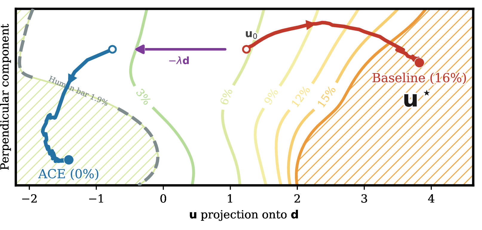
We trace the defect to its mechanism rather than stop at the symptom. Like audio feedback, this self-conditioning loop settles on whatever is most self-predictable, which is repeated content. Two probes pin this down. Turning the feedback strength up, with nothing else changed, drives repetition up and Gen-PPL down together (§3): the loop creates the repetition the metric then rewards. And linearizing the loop, its Jacobian has a single slowest-contracting mode, so the repeated state is a one-dimensional contractive attractor along one direction \(\boldsymbol{d}\) (Fig. 1; §4), a basin that sharper sampling only deepens. This is specific to self-conditioned continuous DLMs (ELF, Plaid [6]), and its one-dimensional geometry is exactly what makes a one-dimensional fix possible.
Because the attractor is one-dimensional, one direction is enough to escape it. ACE (Attractor-Contrast-Escape)1 subtracts that single direction \(\boldsymbol{d}\) from the fed-back estimate at every step. The direction is recovered label-free, as the difference of means of the feedback between trajectories trapped in the basin (top-repetition tertile) and those that stay free (bottom tertile): no per-token labels, no auxiliary model, no retraining. Crucially ACE acts where the defect is born, on the self-conditioning feedback rather than at token selection, because repetition is set in the continuous latent, upstream of that selection, so decode-time fixes are poorly placed to reach it. A single frozen direction, estimated once on the smallest model within a closed-form usable window (§4), cuts repetition to near the human level at competitive quality and transfers near-unchanged across inference knobs and model sizes (cosine \(0.82\)–\(0.96\) to the per-config re-estimate); the same recipe recovers useful directions on other architectures (Plaid, LangFlow [7]).
Evaluating the fix needs care, since Gen-PPL is fooled by the very repetition ACE removes. We therefore accept text under a human repetition bar, read quality on the accepted set with standard reference-free metrics (§3), and measure the compute needed to reach genuinely non-repetitive text (§5); under this evaluation ACE makes human-clean text \(1.5\)–\(5\times\) cheaper at competitive quality.
1.0.0.1 Contributions.
Gen-PPL rewards repetition. Continuous DLMs repeat far more than human text; we show that Gen-PPL, the field’s headline metric, rewards rather than penalizes this and even reverses the model ranking, and we propose a defect-controlled evaluation that accepts text under a human-repetition bar and scores compute-to-clean instead of Gen-PPL (§3, §5).
Its mechanism: an effectively one-dimensional attractor. By direct ablation and a linear-stability analysis we trace the repetition to an effectively one-dimensional contractive attractor of the self-conditioning loop along one direction \(\boldsymbol{d}\) (§4).
Its fix: one frozen direction (ACE). A single cheap, label-free, frozen direction, applied within a closed-form usable steering window, removes most repetition and transfers across knobs and scales, with the same recipe recovering useful directions on other architectures; under our evaluation it reaches human-clean text at comparable quality and \(1.5\)–\(5\times\) lower cost (§5, §6).
1.0.0.2 Relation to prior work.
Prior work exposes metric pathologies in (diffusion-)LM evaluation [8]–[10] or studies discretization and decoding bottlenecks [11], [12]; autoregressive-degeneration work studies repetition along token-time [4], [5]; and steering work shows low-dimensional interventions can control diffusion-LM behavior [13]. We connect these lines: we surface a text-visible repetition defect in self-conditioned continuous DLMs, trace it to the self-conditioning feedback loop, and remove it with a single label-free feedback-direction intervention (full discussion in App. 15).
2 Background and metrics↩︎
2.1 ELF, self-conditioning, and the two samplers↩︎
ELF [2] is a continuous-embedding flow-matching language model. Generation starts from Gaussian noise \(\boldsymbol{z}_0\) and follows a trajectory \(t\in[0,1]\) from noise (\(t{=}0\)) to the clean text embedding (\(t{=}1\)), which is read out to token ids by an independent per-position \(\arg\max\). Two samplers are used: ODE (deterministic Euler integration) and SDE (Euler steps interleaved with partial noise re-injection, governed by the sampler’s rate parameter \(\gamma\), which we call the churn after the analogous stochastic-sampler knob of [14]).
Self-conditioning [1] is a refinement trick for diffusion sampling: instead of predicting the clean data \(\hat{\boldsymbol{x}}\) from the noised input alone, each step feeds back its previous estimate as an extra input and refines it. It adds no extra forward pass, improves sample quality, and is widely used in continuous DLMs (ELF, Plaid [6], LangFlow [7]). Formally it turns the denoiser into a recurrence driven toward a fixed point, the view our analysis builds on (§4).
ELF reuses this same channel to distill classifier-free guidance: instead of two forward passes per step, it feeds the previous estimate \(\hat{\boldsymbol{x}}_{\text{prev}}\) back together with a scalar SC-CFG scale \(w\), and a single pass produces the guided velocity. At each step \(i\), \[\boldsymbol{v}_i = f_\theta\big(\boldsymbol{z}_i,\,t_i,\,w,\,\hat{\boldsymbol{x}}_{\text{prev}}\big), \qquad \hat{\boldsymbol{x}}_{\text{prev}} \leftarrow \hat{\boldsymbol{x}}_i .\] This loop propagates the model’s commitment across later steps and is central to the repetition defect.
2.2 The reported metrics↩︎
Generative perplexity (Gen-PPL) under GPT-2 Large is the standard metric for unconditional DLM evaluation. For a generated text \(\boldsymbol{x}{=}(x_1,\dots,x_N)\), \[\mathrm{\small PPL}(\boldsymbol{x}) = \exp\!\Big(\!-\tfrac{1}{N}\textstyle\sum_{i=1}^{N} \log p_{\text{GPT-2}}(x_i \mid x_{<i})\Big),\] aggregated at corpus level. Unigram entropy is reported as a check against trivial collapse. Crucially, no \(n\)-gram repetition metric is reported in the original ELF paper or in most DLM benchmarks: the gap this paper fills.
2.3 The repetition metric↩︎
We use the standard \(4\)-gram self-repetition rate, the fraction of \(4\)-gram occurrences in a text that duplicate an earlier one: \[\mathrm{\small
rep}_4(\boldsymbol{x}) = \frac{\sum_{g\in\mathcal{G}}\max(c_{\boldsymbol{x}}(g)-1,\,0)}{|\mathcal{G}|},\] with \(\mathcal{G}\) the multiset of \(4\)-grams and \(c_{\boldsymbol{x}}(g)\) its counts. This is identical to seq-rep-4 [5] (the same duplicate \(n\)-gram family, complementary to diversity metrics [15], [16]); we tokenize by whitespace and report the median over samples, with the human-clean acceptance threshold calibrated to human text rather than an arbitrary constant (§3).
3 The repetition defect: Gen-PPL ranks ELF backwards↩︎
ELF’s record-low generative perplexity comes largely from repetition that the metric rewards rather than penalizes. We study the ELF series [2] of
unconditional OpenWebText [17] models at the \(64\)-step, \(\gamma{=}1.0\) operating point (SC-CFG \(w{=}3\)), measuring the defect metric of §2 over \(n{=}1000\) samples per model
against \(n{=}1000\) human (BBC/XSum [18]) articles (Table 1). No authoritative
per-sample cutoff for “degenerate” exists, so we calibrate to these: their seq-rep-4 has median \(0.00\%\) and \(95\)th percentile \(1.92\%\),
the human-clean bar.2 A sample is human-clean when its seq-rep-4 is under this bar, and we read two quantities off it: the accept rate (the share of samples
below it) and clean-PPL (the Gen-PPL of the accepted samples alone, so repetition can no longer lower it). Clean-PPL is a guardrail against passing the bar with diverse nonsense, not the quality verdict, which rests on the reference-free signals
in Table 1 (grammatical acceptability and within-text diversity).
| defect: full \(1000\)-pool | quality: clean accepted set, length-matched | ||||||||
|---|---|---|---|---|---|---|---|---|---|
| 3-5(lr)6-10 Model | rep % \(\downarrow\) | accept \(\uparrow\) | G-PPL \(\downarrow\) | c-PPL \(\downarrow\) | CoLA \(\uparrow\) | dist-\(1\) \(\uparrow\) | dist-\(3\) \(\uparrow\) | s-BLEU \(\downarrow\) | |
| ELF-B (\(105\)M) | base | \(6.83\) | \(0.07\) | \(19.5\) | \(27.7\) | \(0.90\) | \(0.53\) | \(0.97\) | \(0.09\) |
| steer | \(2.11\) | \(0.45\) | \(27.4\) | \(30.6\) | \(0.90\) | \(0.53\) | \(0.97\) | \(0.15\) | |
| ELF-M (\(342\)M) | base | \(1.89\) | \(0.51\) | \(22.1\) | \(25.4\) | \(0.92\) | \(0.55\) | \(0.97\) | \(0.07\) |
| steer | \(0.67\) | \(0.88\) | \(25.5\) | \(26.1\) | \(0.92\) | \(0.56\) | \(0.98\) | \(0.10\) | |
| ELF-L (\(652\)M) | base | \(1.66\) | \(0.56\) | \(24.0\) | \(26.2\) | \(0.91\) | \(0.56\) | \(0.98\) | \(0.07\) |
| steer | \(0.71\) | \(0.84\) | \(27.1\) | \(28.5\) | \(0.91\) | \(0.58\) | \(0.98\) | \(0.10\) | |
| Human (BBC) | \(0.00\) | \(0.95\) | \(13.8\) | \(14.4\) | \(0.89\) | \(0.61\) | \(0.99\) | \(0.05\) | |
4pt
3.0.0.1 The defect, and the backwards ranking.
ELF’s output carries a defect absent from human text yet invisible to the metrics certifying it: heavy \(4\)-gram self-repetition, common in ELF and near-absent in human prose (Table 1; [5]). The ranking it produces runs backwards: Gen-PPL places the smaller ELF-B above the larger ELF-M, yet our defect-controlled clean-PPL reverses them. Strip the repetition and ELF-M is the better model; ELF-B led only because it repeats most: repeated text is trivially predictable, so the GPT-2 scorer assigns it high probability and a flatteringly low Gen-PPL. This is not a measurement artifact (controls in App. 13); a side-by-side example of the defect and the fix is in App. 14 (Table 16).
3.0.0.2 Self-conditioning creates the repetition that Gen-PPL rewards.
Feeding back an attenuated estimate \(\alpha\hat{\boldsymbol{x}}\) and turning \(\alpha\) from \(0\) (feedback off) up to \(1\) (full), with nothing else changed,3 drives repetition up and Gen-PPL down together: the metric calls the generator more than four times “better” just as it grows most repetitive (Table 2). Acceptance under the human bar collapses as \(\alpha\) rises: the Gen-PPL gain is part real fluency and part rewarded repetition, which the metric cannot tell apart.
| \(\alpha\) (SC strength) | \(0.0\) (off) | \(0.3\) | \(0.5\) | \(0.7\) | \(0.9\) | \(1.0\) (full) |
|---|---|---|---|---|---|---|
| rep median % | \(0.00\) | \(0.50\) | \(1.95\) | \(4.57\) | \(6.44\) | \(6.83\) |
| accept | \(1.00\) | \(0.94\) | \(0.49\) | \(0.18\) | \(0.09\) | \(0.07\) |
| Gen-PPL \(\downarrow\) | \(97.5\) | \(48.3\) | \(29.6\) | \(21.7\) | \(19.6\) | \(19.5\) |
| clean-PPL \(\downarrow\) | \(97.5\) | \(49.3\) | \(34.0\) | \(29.2\) | \(27.6\) | \(27.7\) |
4 Mechanism: repetition is a one-dimensional attractor of the self-conditioning loop↩︎
The ablation of §3 identifies the self-conditioning feedback as a causal driver of repetition; we next ask whether that effect is diffuse or concentrated: does the loop’s drift lie along one identifiable direction that predicts a sample’s repetition and, when subtracted, suppresses it? We find that it does: repetition is a contracting attractor of the self-conditioning loop that amplifies the most self-predictable signal, repeated content, and is drawn toward a repetition fixed point \(\boldsymbol{u}^\star\) (Fig. 1). An idealized linear model of this attractor predicts the failure is one-dimensional, repetition living on one slow mode \(\boldsymbol{v}_1\) separable from the benign denoising that writes the text; we then test each prediction against measurement (the formal statements, and the idealizing assumptions they rest on, are in App. 8). The cheap direction \(\boldsymbol{d}\) that exploits it is §5; its transfer across knobs and sizes is §6.
4.0.0.1 The loop splits into a self-conditioning response and a denoising drive.
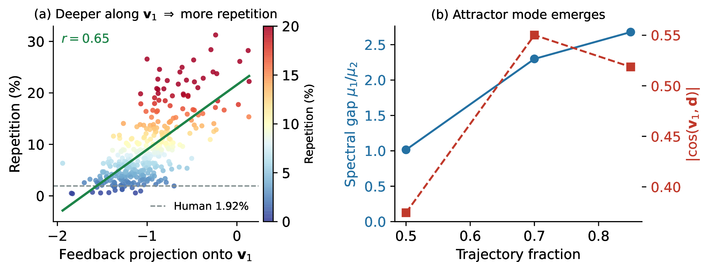
ELF denoises by self-conditioning: each step \(k\) feeds the model its own previous clean-latent estimate \(\hat{\boldsymbol{x}}_k\in\mathbb{R}^{L\times e}\) and reads off the next; iterating this feedback is the loop [1]. We track its position pool (\(e\) the embedding dimension, \(L\) the length), \[\boldsymbol{u}_k \;=\; \tfrac{1}{L}\textstyle\sum_{l=1}^{L}\hat{\boldsymbol{x}}_k[l]\;\in\;\mathbb{R}^{e}, \qquad \boldsymbol{u}_{k+1} \;=\; g(\boldsymbol{u}_k) \;=\; \underbrace{\boldsymbol{s}(\boldsymbol{u}_k)}_{\text{self-conditioning}}+\underbrace{\boldsymbol{f}_k}_{\text{denoising drive}}. \label{eq:scmap}\tag{1}\] One step \(g\) splits in two: the self-conditioning response \(\boldsymbol{s}(\boldsymbol{u}_k)\), how the next estimate depends on the fed-back one (the channel by which repeated content reinforces itself), and the denoising drive \(\boldsymbol{f}_k\), the ordinary denoising the step would do with the feedback off (set by the noise level \(t_k\) and latent \(\boldsymbol{z}_k\)), which carries the bulk of the motion and writes the text. Repetition is governed mainly by \(\boldsymbol{s}\), with only the small on-axis component of \(\boldsymbol{f}_k\) setting the driven offset; \(\boldsymbol{f}_k\) is otherwise the benign carrier it rides on. App. 8 derives the split from the model’s clean-latent prediction \(\boldsymbol{X}_\theta\) (the fed-back \(\hat{\boldsymbol{x}}\) of §2) by a first-order expansion, pooling the feedback over positions into a tractable \(e\)-dimensional state whose link to text-level repetition is empirical (Fig. 2a).
Assumption 1 (Repetition attractor). The self-conditioning map \(\boldsymbol{s}\) has a fixed point \(\boldsymbol{u}^\star\) (repeated content) and is \(C^1\) near it with a contracting Jacobian \(\boldsymbol{J}=\mathrm{D}\boldsymbol{s}(\boldsymbol{u}^\star)\). For the analysis we idealize \(\boldsymbol{J}\) as symmetric, with orthonormal eigenvectors \(\{\boldsymbol{v}_i\}\) and real eigenvalues \(1>\mu_1\ge\mu_2\ge\cdots\ge0\). The leading eigenvector \(\boldsymbol{v}_1\) is the repetition axis, and \(\rho:=1-\mu_1\in(0,1)\) its contraction rate.
The symmetry idealization is used only to decouple the \(\boldsymbol{v}_1\) coordinate into the scalar recursion below; the measured finite-difference \(\boldsymbol{J}\) is only approximately symmetric (App. 9), so the theory reads as a local scalar approximation. The axis \(\boldsymbol{v}_1\) is slowest only relative to the faster off-axis modes, not near-marginal (measured \(\mu_1{\approx}0.15\)).
4.0.0.2 Repetition is one-dimensional.
Linearizing \(\boldsymbol{s}\) about \(\boldsymbol{u}^\star\), its response contracts fastest off, slowest along, the leading eigenvector \(\boldsymbol{v}_1\), so the per-step change decomposes as \[\Delta\boldsymbol{u}_k \;\approx\; \underbrace{\underset{\text{leading}}{\beta_k\,\boldsymbol{v}_1}\;+\;\underset{\text{decays}}{\boldsymbol{r}_k}}_{\text{repetition mode}} \;+\; \underbrace{\boldsymbol{f}_k}_{\text{denoising drive}} \label{eq:decomp}\tag{2}\] (Lemmas 1–2, App. 8): the repetition mode \(\beta_k\boldsymbol{v}_1\) along the axis (coefficient \(\beta_k=-\rho\,a^{(1)}_k\), with \(a^{(1)}_k=\langle\boldsymbol{u}_k-\boldsymbol{u}^\star,\boldsymbol{v}_1\rangle\) the repetition level, how far the feedback sits along \(\boldsymbol{v}_1\)), the subordinate off-axis modes \(\boldsymbol{r}_k\perp\boldsymbol{v}_1\) (the same self-conditioning response on the faster-contracting directions), and the near-orthogonal drive \(\boldsymbol{f}_k\). Because \(\boldsymbol{v}_1\) contracts the slowest (spectral gap \(\mu_1/\mu_2\)), the off-axis transients in \(\boldsymbol{r}_k\) die out faster than the \(\boldsymbol{v}_1\) component, so the structured residual concentrates on \(\boldsymbol{v}_1\): repetition is effectively one-dimensional along this axis. Freezing the drive (\(\boldsymbol{f}_k\equiv\boldsymbol{f}\)), the repetition level settles at \[\boldsymbol{u}_\infty \;=\; \boldsymbol{u}^\star + (\boldsymbol{I}-\boldsymbol{J})^{-1}\boldsymbol{f} \label{eq:driven-fp}\tag{3}\] (Lemma 3, App. 8): the distance \(|a^{(1)}_\infty|=|f^{(1)}|/\rho\) along the axis is the driven offset, the small drive component \(f^{(1)}=\langle\boldsymbol{f},\boldsymbol{v}_1\rangle\) divided by the contraction rate \(\rho\), largest along \(\boldsymbol{v}_1\) since \(\boldsymbol{v}_1\) has the smallest \(1-\mu_i\); the faster off-axis modes settle at smaller offsets.
4.0.0.3 The repetition axis is real and dominant.
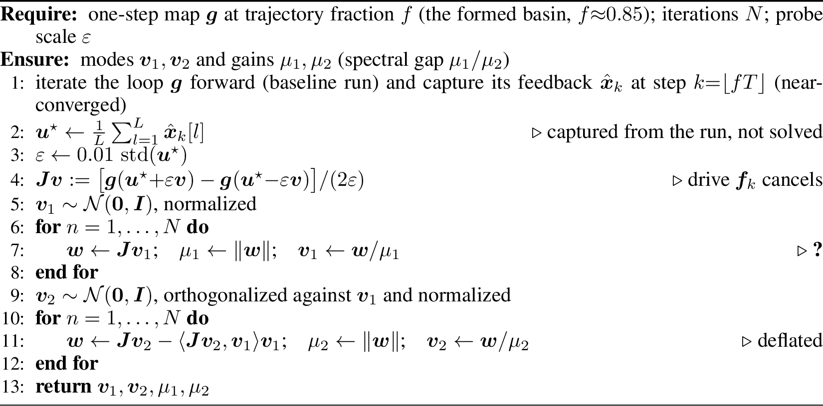
The measured loop bears this out. As the basin forms the spectral gap \(\mu_1/\mu_2\) rises, \(\boldsymbol{v}_1\) becoming the clearly dominant mode (Fig. 2b, Tab. 9); a sample’s repetition level \(a^{(1)}\) predicts its final repetition (Fig. 2a); and the cheap difference-of-means \(\boldsymbol{d}\) (§5) aligns with \(\boldsymbol{v}_1\), the overlap \(\lvert\cos(\boldsymbol{v}_1,\boldsymbol{d})\rvert\) climbing to \(0.55\) as the basin forms (Fig. 2b). Here \(\boldsymbol{d}\) need not equal the single-point eigenvector \(\boldsymbol{v}_1\): it is a trajectory-averaged steering direction that partially aligns with \(\boldsymbol{v}_1\) yet steers better (Tab. 5) by integrating the basin-entry drift over the whole trajectory. Repetition concentrates on this one mode: the defect is effectively one-dimensional. We obtain \(\boldsymbol{v}_1\) and the spectral gap from the feedback Jacobian (Alg. 6).
5 ACE: one subtracted direction escapes the attractor↩︎
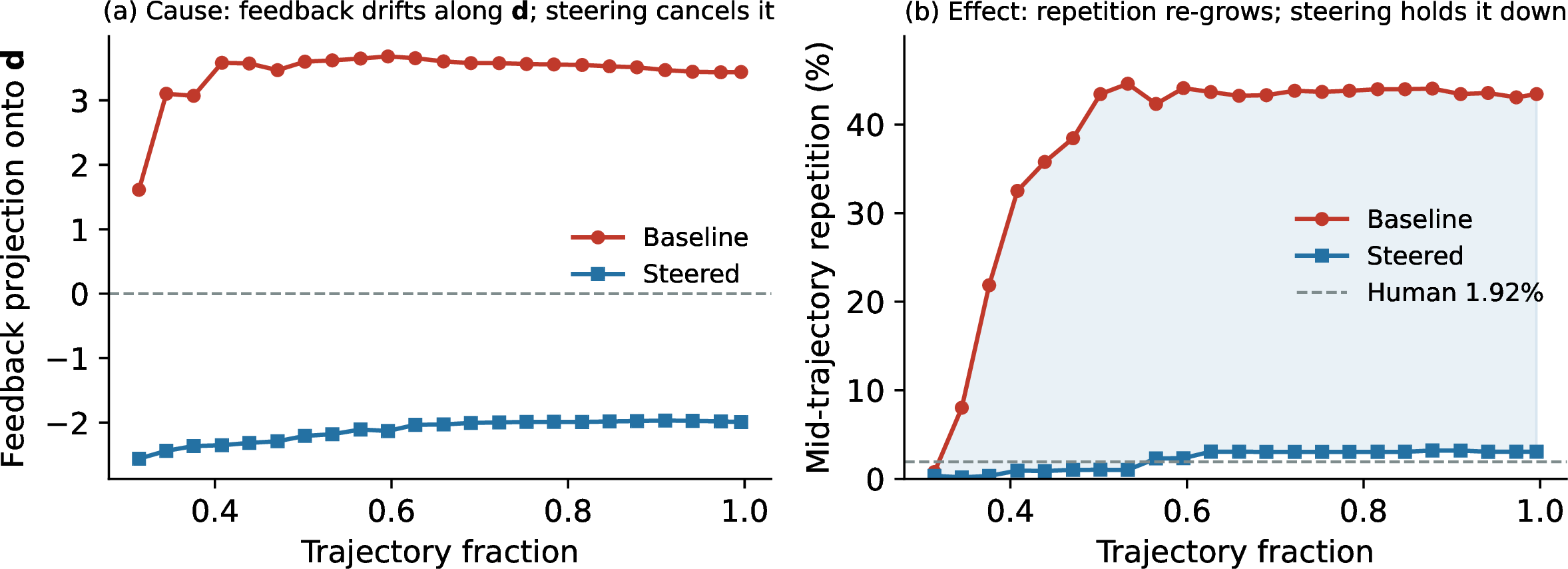
The mechanism is prescriptive (§4): if repetition is a single direction in the fed-back estimate, subtract only that direction and keep the rest. We call this ACE (Attractor-Contrast-Escape): Contrast the average self-conditioning feedback of repetitive vs.non-repetitive trajectories to get the attractor direction \(\boldsymbol{d}\) (a difference of means, in the spirit of activation steering), then Escape by steering against it. This is principled, not heuristic: from just two class means, \(\boldsymbol{d}\) recovers the mechanism’s mode \(\boldsymbol{v}_1\) under an idealized separability model (Prop. 1, App. 8) and empirically aligns with the measured dominant mode. Algorithm 3 instantiates it.

5.1 Main results: repetition and quality↩︎
5.1.0.1 One frozen direction cuts repetition at competitive quality.
At the operating point \(\lambda{=}2\) (the cross-size result, Tab. 1; full dose sweep Tab. 13), steering cuts median repetition to near the human level at competitive clean-PPL, with reference-free quality preserved (grammaticality and within-text diversity): the targeted subtraction keeps the rest of the feedback intact. That a single difference-of-means direction recovers most of the gap is direct evidence the repetition signal is one-dimensional and separable from coherence. Steering is one causal intervention on \(\boldsymbol{d}\) (at inference, Fig. 4); a training-time intervention confirms it: an anti-attractor regularizer on the \(\boldsymbol{d}\)-component of the feedback lowers plain repetition from \(6.8\%\) to \(3.3\%\) at a small clean-PPL cost (\(27.9{\to}29.1\) vs.the matched continue-train control), while the same fine-tune without the penalty barely moves it (Table 3; recipe in App. 12).
| Variant | rep % | accept | Gen-PPL | clean-PPL |
|---|---|---|---|---|
| Original checkpoint | \(6.8\) | \(0.07\) | \(19.5\) | \(27.4\) |
| Continue-train | \(6.4\) | \(0.08\) | \(20.0\) | \(27.9\) |
| Anti-attractor reg | \(\mathbf{3.3}\) | \(0.24\) | \(25.4\) | \(29.1\) |
5.1.0.2 The steer is bounded: a usable dose window.
Subtracting \(\lambda\boldsymbol{d}\) escapes only within a closed-form window \([\lambda^\star,\lambda_{\max}]\) (Prop. 2, App. 8); \(\lambda{=}2\) is the operating point inside it (Tab. 13, Fig. 8). Below it the dose is too weak and repetition is not cut; above it repetition stays low but two costs appear: the perturbed latent leaves the real-token manifold and the text decodes to non-words, an observable proxy for leaving the manifold (the rate spiking by \(\lambda{\approx}8\), Fig. 8), and the accepted text turns generic (self-BLEU climbs with \(\lambda\), Tab. 13).
5.1.0.3 Why steering keeps quality competitive.
The drive \(\boldsymbol{f}_k\) is large but nearly orthogonal to \(\boldsymbol{d}{\approx}\boldsymbol{v}_1\) (Prop. 1; App. 8). ACE subtracts only \(\lambda\boldsymbol{d}\), so it cancels repetition while leaving the text-writing drive intact, dropping repetition to near the human bar at competitive reference-free quality (Tab. 1), with self-BLEU the only mild cost.
5.2 Compute-to-clean comparison↩︎
5.2.0.1 ACE beats every feedback-side alternative we test, and makes clean text cheap.
We benchmark the four routes to less repetition on a common, hard-to-game footing: a reject-to-\(N\) loop scored by compute (NFE) and clean-PPL (Tab. 4; each route defined in App. 11). ACE is the only one both cheap and clean; each alternative fails one axis. Rejecting full-SC post hoc is clean but expensive, its accepts scarce because the low Gen-PPL is the very repetition the bar removes. Disabling self-conditioning (SC-reset) is cheap but decodes to the diverse nonsense the clean-PPL guard exists to catch. Soft-SC either barely cuts repetition or sacrifices coherence to remove it. ACE instead subtracts one direction and leaves the rest of the feedback intact, reaching human-clean text at competitive clean-PPL and \(1.5\)–\(5\times\) cheaper than full-SC rejection across sizes (Fig. 9).
| Method | rep % | NFE | clean-PPL |
|---|---|---|---|
| Human (reference) | \(0.00\) | – | \(14.4\) |
| Full-SC \(+\) reject | \(6.82\) | \(1040\) | \(27.6\) |
| SC-reset | \(0.00\) | \(65\) | \(97.4\) |
| soft-SC mag (\(\alpha{=}0.5\)) | \(1.94\) | \(138\) | \(34.5\) |
| soft-SC noise (\(\sigma{=}0.2\)) | \(6.15\) | \(997\) | \(27.8\) |
| ACE, \(\lambda{=}2\) (ours) | \(2.11\) | \(144\) | \(30.3\) |
6pt
| Direction (\(\lambda{=}2\)) | rep % | clean-PPL |
|---|---|---|
| Baseline (unsteered) | \(6.83\) | \(27.7\) |
| ACE (diff.-of-means \(\bm{d}\)) | \(\mathbf{2.11}\) | \(30.6\) |
| LDA | \(2.29\) | \(29.6\) |
| Logistic | \(3.25\) | \(31.2\) |
| Top-PC (unsup.) | \(5.87\) | \(33.3\) |
| Jacobian \(\bm{v}_1\) | \(5.03\) | \(23.9\) |
Two ablations isolate the remaining choices, the direction and the dose.
5.3 Ablations: direction and dose↩︎
5.3.0.1 The direction: \(\boldsymbol{d}\) matches or beats every estimator.
In the idealized separability model the difference of means coincides with two theory-optimal directions at once, the dynamical optimum \(\boldsymbol{v}_1\) (Prop. 1) and the Fisher discriminant [19], and it stays cheap and robust: where those would need the loop’s Jacobian eigenvector or a noisy high-dimensional covariance inverse, \(\boldsymbol{d}\) reads off only two class means. It matches or beats every alternative at the operating point (Tab. 5): a regularized LDA, the optimal linear discriminant, only matches it, and \(\boldsymbol{d}\) is in fact its simpler isotropic special case; the unsupervised top-PC and Jacobian eigenvector steer worse. The Jacobian eigenvector’s lower clean-PPL is not a quality win: its direct-generation repetition stays high (\(5.03\%\)), so its accepted set is a small filtered subset rather than a fix. The direction itself is robustly recoverable: \(\cos\) to \(\boldsymbol{d}\) stays in \([0.97,1.00]\) across tertile fractions and step windows and collapses to near zero for random or label-permuted controls (Tab. 7). A black-box search lowers repetition only slightly further (\(1.85\) vs \(2.11\)) at \({\sim}8\times\) the cost and along essentially the same axis (\(\cos{\approx}0.92\)) (Tab. 10); this cheap, label-free difference-of-means direction is thus near-optimal.
5.3.0.2 The dose: a fixed \(\lambda\) beats exact projection.
Per-step projection (subtract the instantaneous \(\boldsymbol{d}\)-component, \(\hat{\boldsymbol{x}}_k-\langle\hat{\boldsymbol{x}}_k,\boldsymbol{d}\rangle\boldsymbol{d}\)) is the apparently optimal dose, removing exactly the offending component so it can never over-steer; yet it under-doses, because the loop re-amplifies that component before the next step, and a fixed \(\lambda{\approx}2\) that pre-compensates the amplification does better (Tab. 8). The dose matches the loop’s Jacobian gain to an order of magnitude; the full sweep and usable window are in App. 10.2.
6 The defect and the fix generalize across knobs, sizes, and models↩︎
We test whether the steering fix of §5 is an artefact of one configuration, and whether the underlying repetition defect is specific to ELF. Neither holds.
6.0.0.1 Steering generalizes across every inference knob.
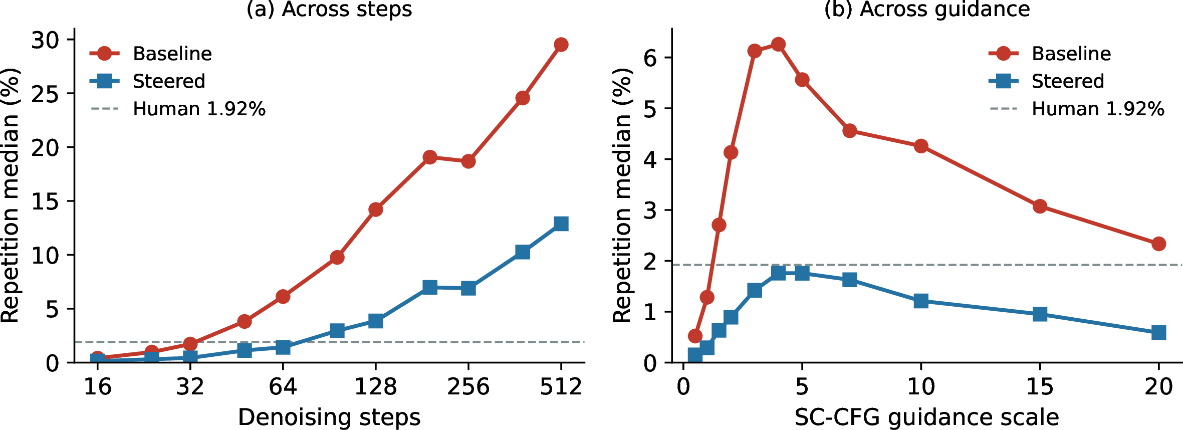
Steering at \(\lambda{=}2\) drops repetition under every inference knob: across denoising steps and guidance scale, the two basin-deepening knobs in Figure 5, and across the remaining knobs (noise scale, SDE/ODE sampler, SDE churn \(\gamma\), and an \(8\)-seed robustness band) at competitive clean-PPL (Table ¿tbl:tab:crosssize?).
6.0.0.2 Cross-model: the direction transfers to other self-conditioned LMs.
The same difference-of-means procedure recovers a steerable attractor direction on other continuous-latent diffusion LMs, so the mechanism is not ELF-specific (Table 6). On LangFlow and the same-recipe Plaid [6], both soft self-conditioning hints like ELF’s, the same recipe transfers: it cuts LangFlow’s repetition outright and Plaid’s heavy-repetition tail.
| base \(\to\) steer | ||||
|---|---|---|---|---|
| 2-5 Model | rep % (median) | rep \(>\) 5 % | Gen-PPL | clean-PPL |
| LangFlow | \(0.92\to\mathbf{0.27}\) | \(20.3\to\mathbf{6.3}\) | \(36.8\to44.2\) | \(44.6\to46.8\) |
| Plaid | \(0.77\to\mathbf{0.73}\) | \(16.0\to\mathbf{10.2}\) | \(19.5\to20.2\) | \(22.5\to22.3\) |
5pt
6.0.0.3 Highlight: one direction, estimated once, transfers across every knob and size, tuning-free.
A single ELF-B direction \(\boldsymbol{d}_B\), estimated once from a few hundred unlabeled samples on the smallest model, steers near-natively across all four inference knobs (steps, guidance, churn, noise) and across model sizes ELF-B/M/L (Table ¿tbl:tab:crosssize?): cosine \(0.82\)–\(0.96\) to the natively re-estimated axis across knobs, \(0.85\)–\(0.88\) across sizes. So \(\boldsymbol{d}\) is a property of the model family, not of the size or operating point, and one \(\boldsymbol{d}\) suffices. That a single direction steers every size hints the attractor is not a per-checkpoint quirk but a systematic bias of the self-conditioned training recipe, set by the shared paradigm rather than learned afresh at each scale.
7 Conclusion↩︎
We showed that the headline metric of self-conditioned (continuous) diffusion language models rewards repetition: ELF’s low Gen-PPL comes mostly from repetition it rewards, so on Gen-PPL the \(105\)M model outranks the \(342\)M one that beats it once repetition is controlled. We traced this to its source, a contractive fixed point of the self-conditioning loop that forms a one-dimensional basin, and turned that mechanism into a fix. We propose ACE (Attractor-Contrast-Escape): it recovers the basin’s direction \(\boldsymbol{d}\) once by a difference of means and subtracts it from the feedback; this removes most repetition, transfers across samplers and model sizes, and is partly internalizable by training. Since Gen-PPL rewards the very repetition ACE removes, we score the fix on a compute-to-clean evaluation against a human repetition floor, where it reaches genuinely non-repetitive text at competitive clean-PPL and \(1.5\)–\(5\times\) lower cost. That one direction serves every model size points to a defect of the self-conditioned paradigm itself rather than any single checkpoint, and the same construction recovers useful directions on other architectures.
8 Formal analysis and empirical validation↩︎
This appendix develops the idealized linear model of the self-conditioning loop in derivation order, then validates the structure on the trained network. We linearize the loop (Lemma 1), read off the per-step decomposition splitting each update into drive and repetition mode (Lemma 2), and locate where the driven loop settles (Lemma 3). From this we derive the two consequences used in §4: a label-free difference of means recovers the repetition axis (Prop. 1), and subtracting it escapes the basin within a closed-form dose window (Prop. 2). Every displayed result is exact for this idealized model under its stated assumptions (a symmetrized Jacobian, an exogenous drive, and the scalar approximations flagged at each step); the final empirical section then estimates the Jacobian on the real network and checks each prediction against measurement.
8.1 Structure of the linearized loop↩︎
8.1.0.1 Setup: where \(\boldsymbol{s}\), \(\boldsymbol{f}_k\), and \(\boldsymbol{J}\) come from.
We reuse the pooled-feedback loop \(\boldsymbol{u}_{k+1}=g(\boldsymbol{u}_k)\) of equation 1 and Assumption 1, writing \(\overline{(\cdot)}=\tfrac1L\sum_{l=1}^{L}(\cdot)[l]\) for the position pool. One step is the trained model \(\boldsymbol{X}_\theta\) evaluated on its two inputs, the current noisy latent \(\boldsymbol{z}_k\) and the fed-back estimate (taken uniform across positions, the pooling assumption of §4), at noise level \(t_k\): \[g(\boldsymbol{u}_k)\;=\;\overline{\boldsymbol{X}_\theta\!\big([\boldsymbol{z}_k,\,\boldsymbol{u}_k\boldsymbol{1}_L],\,t_k\big)} . \label{eq:gmodel}\tag{4}\] The model sees \(\boldsymbol{u}_k\) only through the fed-back channel, so we expand in that channel about the repetition fixed point \(\boldsymbol{u}^\star\) (Assumption 1): \[\boldsymbol{X}_\theta\!\big([\boldsymbol{z}_k,\boldsymbol{u}_k],t_k\big) \;=\;\underbrace{\boldsymbol{X}_\theta\!\big([\boldsymbol{z}_k,\boldsymbol{u}^\star],t_k\big)}_{\text{zeroth order}} \;+\;\underbrace{\boldsymbol{J}\,(\boldsymbol{u}_k-\boldsymbol{u}^\star)}_{\text{first order}} \;+\;o(\lVert\boldsymbol{a}_k\rVert). \label{eq:taylor}\tag{5}\] The three objects used throughout are the terms of equation 5 : the denoising drive \(\boldsymbol{f}_k:=\overline{\boldsymbol{X}_\theta([\boldsymbol{z}_k,\boldsymbol{u}^\star],t_k)}-\boldsymbol{u}^\star\) (zeroth order: a function of \(\boldsymbol{z}_k,t_k\), constant in \(\boldsymbol{u}_k\)), the self-conditioning Jacobian \(\boldsymbol{J}:=\partial\,\overline{\boldsymbol{X}_\theta}/\partial\boldsymbol{u}\big|_{\boldsymbol{u}^\star}\), and the self-conditioning map \(\boldsymbol{s}(\boldsymbol{u}):=\boldsymbol{u}^\star+\boldsymbol{J}(\boldsymbol{u}-\boldsymbol{u}^\star)+o(\lVert\boldsymbol{u}-\boldsymbol{u}^\star\rVert)\), which fixes \(\boldsymbol{u}^\star\) by construction, \(\boldsymbol{s}(\boldsymbol{u}^\star)=\boldsymbol{u}^\star\). Collecting them gives the split \[g(\boldsymbol{u}_k)\;=\;\boldsymbol{s}(\boldsymbol{u}_k)+\boldsymbol{f}_k . \label{eq:gsplit}\tag{6}\] The one substantive reduction is treating the latent trajectory \(\{\boldsymbol{z}_k\}\) as exogenous, so \(\boldsymbol{f}_k\) acts as a \(\boldsymbol{u}_k\)-independent forcing (its \(\boldsymbol{u}_k\)-dependence beyond linear order is the \(o(\lVert\boldsymbol{a}_k\rVert)\) remainder). Downstream measurements support this: the drive is nearly orthogonal to the repetition axis (\(\lvert\cos(\boldsymbol{f}_k,\boldsymbol{v}_1)\rvert{=}0.15\); App. 8.4) and \(\boldsymbol{J}\) is contracting with a dominant mode aligned to \(\boldsymbol{d}\) (Tab. 9).
Let \(\boldsymbol{a}_k=\boldsymbol{u}_k-\boldsymbol{u}^\star\) be the residual, with coordinates \(a^{(i)}_k=\langle\boldsymbol{a}_k,\boldsymbol{v}_i\rangle\) in the eigenbasis of Assumption 1; by the symmetric-\(\boldsymbol{J}\) idealization \(\boldsymbol{v}_1\) is both a left and right eigenvector, so the \(\boldsymbol{v}_1\)-coordinate decouples below.
Lemma 1 (Linearized loop). Near the fixed point the residual obeys the linear recursion \[\boldsymbol{a}_{k+1}\;=\;\boldsymbol{J}\,\boldsymbol{a}_k+\boldsymbol{f}_k , \label{eq:residrec}\qquad{(1)}\] the residual form of the loop equation 1 near \(\boldsymbol{u}^\star\).
Proof. Subtract \(\boldsymbol{u}^\star\) from the split equation 6 and use \(\boldsymbol{s}(\boldsymbol{u}_k)=\boldsymbol{u}^\star+\boldsymbol{J}\boldsymbol{a}_k+o(\lVert\boldsymbol{a}_k\rVert)\) from equation 5 : \(\boldsymbol{a}_{k+1}=\boldsymbol{J}\boldsymbol{a}_k+\boldsymbol{f}_k+o(\lVert\boldsymbol{a}_k\rVert)\), which is equation ?? once the higher-order remainder is dropped (exact for the idealized linear model). ◻
Lemma 2 (Per-step decomposition). The one-step change splits exactly as \[\Delta\boldsymbol{u}_k\;=\;\beta_k\,\boldsymbol{v}_1\;+\;\boldsymbol{r}_k\;+\;\boldsymbol{f}_k , }\] the decomposition of equation 2 , with repetition coefficient \(\beta_k=(\mu_1-1)\,a^{(1)}_k\) and remainder \(\boldsymbol{r}_k=\sum_{i\ge2}(\mu_i-1)\,a^{(i)}_k\boldsymbol{v}_i\). The drive \(\boldsymbol{f}_k\) is orthogonal to \(\boldsymbol{v}_1\) (off the repetition axis, App. 8.4), and the remainder collects the off-axis modes, which contract faster (\(\mu_i\le\mu_1\) for \(i\ge2\)).
Proof. From Lemma 1, \(\Delta\boldsymbol{u}_k=\boldsymbol{u}_{k+1}-\boldsymbol{u}_k=\boldsymbol{a}_{k+1}-\boldsymbol{a}_k=(\boldsymbol{J}-\boldsymbol{I})\boldsymbol{a}_k+\boldsymbol{f}_k\). Expanding the residual in the orthonormal eigenbasis (Assumption 1), \(\boldsymbol{a}_k=\sum_i a^{(i)}_k\boldsymbol{v}_i\), gives \((\boldsymbol{J}-\boldsymbol{I})\boldsymbol{a}_k=\sum_i(\mu_i-1)a^{(i)}_k\boldsymbol{v}_i\); separating the \(i{=}1\) term as \(\beta_k\boldsymbol{v}_1\) from the rest as \(\boldsymbol{r}_k\) yields the stated identity. Since projecting equation ?? on \(\boldsymbol{v}_i\) gives the scalar recursion \(a^{(i)}_{k+1}=\mu_i a^{(i)}_k+f^{(i)}\), whose homogeneous transient decays as \(\mu_i^k\), fastest for the smallest \(\mu_i\); so the off-axis transients (\(\mu_i\le\mu_1\), \(i\ge2\)) die out at least as fast as the \(\boldsymbol{v}_1\) transient. They do not vanish: each settles at the driven offset \(f^{(i)}/(1-\mu_i)\) (the off-axis content \(\boldsymbol{w}\) of Prop. 1), largest along \(\boldsymbol{v}_1\). So \(\boldsymbol{v}_1\) carries both the slowest transient and the largest steady offset, the persistent structured part of the residual (Lemma 3). ◻
Lemma 3 (Where the driven loop settles). With the drive frozen at \(\boldsymbol{f}_k\equiv\boldsymbol{f}\), the recursion equation ?? converges geometrically (at rate \(\mu_1\)) to the unique fixed point \(\boldsymbol{a}_\infty=(\boldsymbol{I}-\boldsymbol{J})^{-1}\boldsymbol{f}\), i.e. \[\boldsymbol{u}_\infty=\boldsymbol{u}^\star+(\boldsymbol{I}-\boldsymbol{J})^{-1}\boldsymbol{f}. }\] Its distance from \(\boldsymbol{u}^\star\) along the repetition axis is \(\lvert a^{(1)}_\infty\rvert=\lvert f^{(1)}\rvert/(1-\mu_1)=\lvert f^{(1)}\rvert/\rho\) with \(f^{(1)}=\langle\boldsymbol{f},\boldsymbol{v}_1\rangle\). Since \(\boldsymbol{f}\) is near-orthogonal to \(\boldsymbol{v}_1\) (\(f^{(1)}\) small), \(\boldsymbol{u}_\infty\) sits a small but nonzero distance from \(\boldsymbol{u}^\star\): a bounded repetition offset, not full collapse. This \(\lvert f^{(1)}\rvert/\rho\) is a residual offset, not an amplification: stronger contraction (larger \(\rho\), smaller \(\mu_1\)) leaves the drive less room to push the endpoint off \(\boldsymbol{u}^\star\), shrinking the distance and deepening repetition, whereas a near-marginal mode (\(\rho\!\to\!0\)) would let even a small \(f^{(1)}\) hold \(\boldsymbol{u}_\infty\) far from \(\boldsymbol{u}^\star\).
Proof. \(\boldsymbol{J}\) is contracting, so its spectral radius \(\mu_1<1\) and \(\boldsymbol{I}-\boldsymbol{J}\) is invertible (eigenvalues \(1-\mu_i>0\)); the Neumann series \(\sum_{j\ge0}\boldsymbol{J}^j=(\boldsymbol{I}-\boldsymbol{J})^{-1}\) converges. Unrolling equation ?? with \(\boldsymbol{f}_k\equiv\boldsymbol{f}\) from \(\boldsymbol{a}_0\), \[\boldsymbol{a}_k=\boldsymbol{J}^k\boldsymbol{a}_0+\sum_{j=0}^{k-1}\boldsymbol{J}^j\boldsymbol{f}\;\xrightarrow[k\to\infty]{}\;(\boldsymbol{I}-\boldsymbol{J})^{-1}\boldsymbol{f}, \label{eq:unroll}\tag{7}\] the transient \(\boldsymbol{J}^k\boldsymbol{a}_0\) vanishing at rate \(\mu_1^k\). Equivalently \(\boldsymbol{a}_\infty\) solves \((\boldsymbol{I}-\boldsymbol{J})\boldsymbol{a}_\infty=\boldsymbol{f}\); projecting on the unit eigenvector \(\boldsymbol{v}_1\), \((1-\mu_1)a^{(1)}_\infty=f^{(1)}\), so \(\lvert a^{(1)}_\infty\rvert=\lvert f^{(1)}\rvert/(1-\mu_1)\). The map \(\rho\mapsto\lvert f^{(1)}\rvert/\rho\) is decreasing on \((0,1)\), so a larger \(\rho\) shrinks the residual. ◻
8.1.0.2 Nonlinear local existence and uniqueness.
Lemma 3 is exact for the linearized loop; the same conclusion survives for the true nonlinear map by the implicit function theorem. Write the driven fixed-point condition as \(\boldsymbol{G}(\boldsymbol{u},\boldsymbol{f})=\boldsymbol{s}(\boldsymbol{u})-\boldsymbol{u}+\boldsymbol{f}=\boldsymbol{0}\); it is \(C^1\) near \((\boldsymbol{u}^\star,\boldsymbol{0})\) (Assumption 1) with \(\boldsymbol{G}(\boldsymbol{u}^\star,\boldsymbol{0})=\boldsymbol{0}\), and its \(\boldsymbol{u}\)-Jacobian there is \(\partial_{\boldsymbol{u}}\boldsymbol{G}=\boldsymbol{J}-\boldsymbol{I}\), invertible whenever \(\mu_1\neq1\). The contraction \(\mu_1<1\) supplies this (measured \(\mu_1{\approx}0.15\), App. 8.4), so the theorem gives a neighborhood of \(\boldsymbol{f}{=}\boldsymbol{0}\) on which the driven fixed point \(\boldsymbol{u}_\infty(\boldsymbol{f})\) exists, is locally unique, and is \(C^1\) in \(\boldsymbol{f}\), with first-order expansion \(\boldsymbol{u}_\infty(\boldsymbol{f})=\boldsymbol{u}^\star+(\boldsymbol{I}-\boldsymbol{J})^{-1}\boldsymbol{f}+o(\lVert\boldsymbol{f}\rVert)\): the linear formula equation 3 is its leading term. The theorem upgrades the linear solution to a locally unique branch of the nonlinear loop; it does not by itself produce \(\boldsymbol{u}^\star\), whose existence is Assumption 1 and which appears empirically as a near-fixed point (residual \({\approx}0.07\); App. 8.4).
8.1.0.3 Frozen coefficients.
Lemma 3 freezes \(\boldsymbol{J}\) and \(\boldsymbol{f}\) (the standard quasi-static linearization); both vary slowly over a finite budget, so the real trajectory tracks this instantaneous attractor rather than reaching it.
8.2 Consequence 1: a label-free direction recovers the axis↩︎
Definition 1 (Difference-of-means direction and steering). Let \(a^{(1)}=\langle\boldsymbol{a},\boldsymbol{v}_1\rangle\) be the signed repetition-axis coordinate, oriented so \(+\boldsymbol{v}_1\) points toward the repetition fixed point \(\boldsymbol{u}^\star\) and the rep score is monotone increasing* in \(a^{(1)}\) (deeper into the basin along \(+\boldsymbol{v}_1\) is more repetitive). The trapped and free groups \(\mathcal{T},\mathcal{F}\) are the top and bottom repetition tertiles, hence separated along signed \(a^{(1)}\) with \(\bar a^{(1)}_{\mathcal{T}}>\bar a^{(1)}_{\mathcal{F}}\), so the difference-of-means gap \(\bar a^{(1)}_{\mathcal{T}}-\bar a^{(1)}_{\mathcal{F}}\neq0\). The estimator \[\boldsymbol{d}\;=\;\frac{\boldsymbol{m}_{\mathcal{T}}-\boldsymbol{m}_{\mathcal{F}}}{\lVert\boldsymbol{m}_{\mathcal{T}}-\boldsymbol{m}_{\mathcal{F}}\rVert}, \qquad \boldsymbol{m}_{\mathcal{T}}=\mathbb{E}[\boldsymbol{u}\mid\mathcal{T}],\quad \boldsymbol{m}_{\mathcal{F}}=\mathbb{E}[\boldsymbol{u}\mid\mathcal{F}], \label{eq:dmean}\tag{8}\] defines the attractor direction, and steered self-conditioning feeds back \(\tilde{\boldsymbol{x}}_k=\hat{\boldsymbol{x}}_k-\lambda\,\boldsymbol{d}\) with strength \(\lambda\ge0\).*
Proposition 1 (Difference of means recovers the attractor direction). Split the feedback into the repetition axis and the rest, \(\boldsymbol{u}=\boldsymbol{u}^\star+a^{(1)}\boldsymbol{v}_1+\boldsymbol{w}\), where the off-axis content \(\boldsymbol{w}\perp\boldsymbol{v}_1\) collects the drive \(\boldsymbol{f}_k\) and remainder \(\boldsymbol{r}_k\) of Lemma 2 (both \(\perp\boldsymbol{v}_1\)). Assume separability: the trapped/free split acts only through the on-axis coordinate \(a^{(1)}\), so the off-axis \(\boldsymbol{w}\) has a group-independent mean, \(\mathbb{E}[\boldsymbol{w}\mid\mathcal{T}]=\mathbb{E}[\boldsymbol{w}\mid\mathcal{F}]\). Then the difference of means is parallel to the repetition axis, \(\boldsymbol{d}\parallel\boldsymbol{v}_1\) (empirically partial; see the remark).
Proof. Take the group-conditional mean under the model: for \(\mathcal{G}\in\{\mathcal{T},\mathcal{F}\}\), \[\boldsymbol{m}_{\mathcal{G}}=\mathbb{E}[\boldsymbol{u}\mid\mathcal{G}] =\boldsymbol{u}^\star+\bar a^{(1)}_{\mathcal{G}}\,\boldsymbol{v}_1+\mathbb{E}[\boldsymbol{w}\mid\mathcal{G}], \qquad \bar a^{(1)}_{\mathcal{G}}:=\mathbb{E}[a^{(1)}\mid\mathcal{G}],\] the group-mean on-axis coordinate. Subtracting the two groups, \[\boldsymbol{m}_{\mathcal{T}}-\boldsymbol{m}_{\mathcal{F}} =\underbrace{(\boldsymbol{u}^\star-\boldsymbol{u}^\star)}_{=\,\boldsymbol{0}} +\bigl(\bar a^{(1)}_{\mathcal{T}}-\bar a^{(1)}_{\mathcal{F}}\bigr)\boldsymbol{v}_1 +\underbrace{\bigl(\mathbb{E}[\boldsymbol{w}\mid\mathcal{T}]-\mathbb{E}[\boldsymbol{w}\mid\mathcal{F}]\bigr)}_{=\,\boldsymbol{0}} : \label{eq:dmeanderiv}\tag{9}\] the fixed point \(\boldsymbol{u}^\star\) is shared by both groups and cancels, and the off-axis term \(\mathbb{E}[\boldsymbol{w}\mid\mathcal{T}]-\mathbb{E}[\boldsymbol{w}\mid\mathcal{F}]\) vanishes by the modeling assumption. Only the on-axis term survives, so \(\boldsymbol{m}_{\mathcal{T}}-\boldsymbol{m}_{\mathcal{F}}=(\bar a^{(1)}_{\mathcal{T}}-\bar a^{(1)}_{\mathcal{F}})\boldsymbol{v}_1\parallel\boldsymbol{v}_1\), with scalar \(\bar a^{(1)}_{\mathcal{T}}-\bar a^{(1)}_{\mathcal{F}}\neq0\) since the trapped group sits deeper along \(\boldsymbol{v}_1\) (Definition 1). Normalizing, \(\boldsymbol{d}\parallel\boldsymbol{v}_1\) (up to sign). ◻
8.2.0.1 \(\boldsymbol{d}\) is the empirical counterpart of \(\boldsymbol{v}_1\).
The measured alignment is \(\lvert\cos(\boldsymbol{v}_1,\boldsymbol{d})\rvert{\le}0.55\), and \(\boldsymbol{d}\) steers better than the single-point \(\boldsymbol{v}_1\) itself (Tab. 5) because it averages the basin-entry drift over the trajectory and many samples. We take Prop. 1 as the idealized motivation and \(\boldsymbol{d}\) as the operational direction.
8.3 Consequence 2: a closed-form steering window↩︎
Proposition 2 (Steering threshold and usable window). Apply Definition 1 with \(\boldsymbol{d}=\boldsymbol{v}_1\) (Prop. 1). Track the signed axis coordinate \(c_k=\langle\boldsymbol{u}_k-\boldsymbol{u}^\star,\boldsymbol{v}_1\rangle\) (the signed \(a^{(1)}\) of Definition 1) and the distance from the repetition fixed point \(D_k=-c_k\ge0\) (\(+\boldsymbol{v}_1\) points toward \(\boldsymbol{u}^\star\), so repetition is proximity to \(\boldsymbol{u}^\star\) and the rep score decreases in \(D_k\)). Projecting the steered recursion on \(\boldsymbol{v}_1\) and retaining* the drive component \(f^{(1)}=\langle\boldsymbol{f},\boldsymbol{v}_1\rangle\) (proof) gives \[c_{k+1}=\mu_1\bigl(c_k-\lambda\bigr)+f^{(1)}, \qquad\text{equivalently}\qquad D_{k+1}=\mu_1\bigl(D_k+\lambda\bigr)+\lvert f^{(1)}\rvert, \label{eq:steeredmap}\tag{10}\] with unique stable steady state \[D_\infty \;=\; \frac{1-\rho}{\rho}\,\lambda \;+\; \frac{\lvert f^{(1)}\rvert}{\rho} . \label{eq:ainf}\tag{11}\] The first term is the steering-induced outward drift; the second is the baseline offset of Lemma 3 (\(D_\infty=\lvert f^{(1)}\rvert/\rho\) at \(\lambda{=}0\)), so steering adds to a nonzero starting distance, not to zero. Let \(a_{\mathrm{crit}}\) be the distance above which the orbit is non-repetitive and \(R\) the local manifold radius. In this steady-state scalar approximation repetition is escaped once \(\lambda\ge\lambda^\star\) and the decode stays on-manifold while \(\lambda\le\lambda_{\max}\), with \[\lambda^\star \;=\; \frac{\rho\,a_{\mathrm{crit}}-\lvert f^{(1)}\rvert}{1-\rho}, \qquad \lambda_{\max} \;=\; \frac{\rho\,R-\lvert f^{(1)}\rvert}{1-\rho}. \label{eq:window}\tag{12}\] Both thresholds lie below their \(f^{(1)}{=}0\) values by \(\lvert f^{(1)}\rvert/(1-\rho)\) (the baseline head start lowers the escape dose), while the usable window \([\lambda^\star,\lambda_{\max}]\) keeps width \((R-a_{\mathrm{crit}})\,\rho/(1-\rho)\). We do not instantiate \(a_{\mathrm{crit}}\), \(R\), or \(f^{(1)}\) on ELF, so the window is qualitative; its numeric range is the empirical \(\lambda\)-sweep of App. 10.2.*
Proof. Steered coordinate. Steering feeds back \(\hat{\boldsymbol{x}}_k-\lambda\boldsymbol{v}_1\), so \(\boldsymbol{a}_{k+1}=\boldsymbol{J}(\boldsymbol{a}_k-\lambda\boldsymbol{v}_1)+\boldsymbol{f}_k\). With \(\boldsymbol{J}\) symmetric (Assumption 1, so \(\langle\boldsymbol{J}\boldsymbol{x},\boldsymbol{v}_1\rangle=\mu_1\langle\boldsymbol{x},\boldsymbol{v}_1\rangle\)), projecting on \(\boldsymbol{v}_1\) and keeping the drive component \(f^{(1)}=\langle\boldsymbol{f}_k,\boldsymbol{v}_1\rangle\) closes the scalar recursion \(c_{k+1}=\mu_1(c_k-\lambda)+f^{(1)}\) of equation 10 , decoupled from the off-axis content. (Lemma 2 dropped \(f^{(1)}\) as small; we retain it here so that \(\lambda{=}0\) recovers the baseline offset \(c_\infty=f^{(1)}/\rho\) of Lemma 3 rather than a collapse to \(\boldsymbol{u}^\star\).) Since \(+\boldsymbol{v}_1\) points toward \(\boldsymbol{u}^\star\) while \(\boldsymbol{a}=\boldsymbol{u}-\boldsymbol{u}^\star\) is the outward displacement, \(c_k\le0\), and the drive points outward (\(f^{(1)}\le0\)); negating gives the distance form \(D_{k+1}=\mu_1(D_k+\lambda)+\lvert f^{(1)}\rvert\), an outward drift forced by \(\boldsymbol{d}\), not assumed.
Steady state. Setting \(D_{k+1}=D_k=D_\infty\) in equation 10 gives \((1-\mu_1)\,D_\infty=\mu_1\lambda+\lvert f^{(1)}\rvert\), so \(D_\infty=(1-\rho)\lambda/\rho+\lvert f^{(1)}\rvert/\rho\) as in equation 11 . Subtracting this relation leaves \(D_{k+1}-D_\infty=\mu_1(D_k-D_\infty)\), decaying as \(\mu_1^{\,k}\) (\(\mu_1<1\)): the steady state is unique and stable on this axis.
Window. \(D_\infty\) grows linearly in \(\lambda\) from the baseline \(\lvert f^{(1)}\rvert/\rho\), clearing \(a_{\mathrm{crit}}\) once \(\lambda\ge\lambda^\star\) and staying below \(R\) while \(\lambda\le\lambda_{\max}\): \[D_\infty\ge a_{\mathrm{crit}}\iff\lambda\ge\lambda^\star, \qquad D_\infty\le R\iff\lambda\le\lambda_{\max},\] with \(\lambda^\star,\lambda_{\max}\) as in equation 12 (each inequality solved for \(\lambda\)). ◻
Equation equation 12 is the formal content of our empirical picture: steering removes the pull into the basin without touching the off-\(\boldsymbol{v}_1\) content \(\boldsymbol{w}\) that blanket soft-SC attenuates indiscriminately (§5); a finite window \([\lambda^\star,\lambda_{\max}]\) exists (Fig. 8), with \(\lambda{\approx}2\) the conservative knee (repetition is monotone-decreasing in \(\lambda\) through \(\lambda{\approx}4\), so \(\lambda{\approx}2\) is the smallest comfortably-delivering dose, not the rep-minimizer) and over-steering past the upper edge eventually spiking non-words (by \(\lambda{\approx}8\)) as predicted by \(\lambda_{\max}\) (Fig. 8).
8.4 Empirical validation on the trained loop↩︎
8.4.0.1 Existence, contraction, and local uniqueness of the fixed point.
We test the premises of Assumption 1 and the implicit-function note of App. 8.1 directly on the trained loop. Freezing \((\boldsymbol{z}_k,t_k)\) at the formed basin (fraction \(0.85\)) and iterating the full step \(\boldsymbol{u}\!\leftarrow\!\boldsymbol{g}(\boldsymbol{u})\) from the captured base point, the relative residual \(\lVert\boldsymbol{g}(\boldsymbol{u})-\boldsymbol{u}\rVert/\lVert\boldsymbol{u}\rVert\) starts at \(0.07\) and settles near \(0.06\), the floor set by the step’s sampling noise: \(\boldsymbol{g}\) has a near-fixed point, and the captured base point already sits on it (pooled \(\boldsymbol{u}^\star\) captured vs.iterated, \(\cos{=}1.00\)). Power-iterating the Jacobian there gives a leading gain \(\mu_1{\approx}0.15<1\) (captured and strictly-iterated base points agree, \(0.148\) vs.\(0.149\)): the loop is contracting, so \(\boldsymbol{I}-\boldsymbol{J}\) is invertible, the implicit-function premise (\(\mu_1\neq1\)) holds, and the driven fixed point is locally unique. The recovered axis is itself stable across the two base points (\(\lvert\cos(\boldsymbol{v}_1^{\mathrm{cap}},\boldsymbol{v}_1^{\mathrm{strict}})\rvert{=}0.999\), and \(0.999\) to the saved \(\boldsymbol{v}_1\) used in Fig. 2), the empirical face of local uniqueness.
8.4.0.2 A dominant contracting mode emerges as the basin forms.
Estimating \(\boldsymbol{J}\) by the matrix-free power iteration of Alg. 6 (\(n{=}100\) trajectories, \(30\) iterations) at base points of increasing convergence (trajectory fraction \(0.5\!\to\!0.85\)), the predicted structure appears: the spectral gap \(\mu_1/\mu_2\) rises from \({\approx}1\) to \(2.7\), one mode separating, and the label-free \(\boldsymbol{d}\) aligns with it (\(\lvert\cos(\boldsymbol{v}_1,\boldsymbol{d})\rvert\) up to \(0.55\), well above the random floor \(1/\sqrt{e}{=}0.044\)), with a perturbation along \(\boldsymbol{d}\) amplified \(2.2\times\) over a random one (Tab. 9). So \(\boldsymbol{d}\) aligns with the measured dominant mode of the loop, the empirical counterpart of the idealized \(\boldsymbol{d}\!\parallel\!\boldsymbol{v}_1\) (Prop. 1), with the alignment only partial; the full estimator anatomy and data efficiency are in App. 9.
8.4.0.3 The drive is off the repetition axis (Lemma 2).
The decomposition \(\Delta\boldsymbol{u}_k=\beta_k\boldsymbol{v}_1+\boldsymbol{r}_k+\boldsymbol{f}_k\) resolves a seeming contradiction. The observed drift is dominated by the denoising drive \(\boldsymbol{f}_k\), so its leading direction (top principal component of \(\Delta\boldsymbol{u}\), noise-averaged and pooled over the late third of steps, \(n{=}200\) trajectories) is near-orthogonal to both the repetition eigenvector (\(\lvert\cos\rvert{=}0.15\), as is the per-step drive itself, \(\lvert\cos(\boldsymbol{f}_k,\boldsymbol{v}_1)\rvert{=}0.15\)) and the steering direction (\(\lvert\cos\rvert{=}0.09\)); but the Jacobian, a derivative, cancels the perturbation-independent \(\boldsymbol{f}_k\) and exposes the self-amplified mode, whose leading eigenvector is \(\boldsymbol{d}\). Drift and Jacobian thus agree rather than conflict, one reading the forcing \(\boldsymbol{f}_k\) and the other the self-amplified mode \(\beta_k\boldsymbol{v}_1\); ACE acts along \(\boldsymbol{d}\perp\boldsymbol{f}_k\), leaving the drive intact (§5).
9 Anatomy of \(\boldsymbol{d}\) (extended)↩︎
This appendix collects the evidence behind §5.
9.0.0.1 One direction across samplers.
A single base-config \(\boldsymbol{d}\) steers across steps, guidance, \(\gamma\), ODE/SDE, noise scales, seeds and model sizes at near-native repetition reduction. Re-estimating \(\boldsymbol{d}\) under each setting recovers nearly the same axis: cosine \(0.82\)–\(0.96\) to \(\boldsymbol{d}_B\) over the knob and size re-estimates of Table ¿tbl:tab:crosssize? (\(0.86\)–\(0.94\) across the step sweep alone; §6). Pooling the feedback over six samplers (\(1500\) trajectories) and re-estimating barely moves it: \(\cos(\boldsymbol{d}_{\mathrm{pooled}}, \boldsymbol{d}_{\mathrm{base}})=0.89\). The direction is thus a property of the model, not the operating point; the optimal strength \(\lambda\) (not the direction) absorbs the configuration dependence.
4pt
@l c c@ c c@ c@ c c@ & & & &
(lr)2-3(lr)4-5(lr)7-8 Config & rep % & clean-PPL & rep % & clean-PPL & \(\cos(\bm{d},\bm{d}_B)\) & rep % & clean-PPL
ELF-M (\(342\)M) & \(2.17\) & \(25.2\) & \(0.54\) & \(29.0\) & \(0.88\) & \(0.67\) & \(26.1\)
ELF-L (\(652\)M) & \(1.58\) & \(26.1\) & \(0.41\) & \(28.9\) & \(0.85\) & \(0.71\) & \(28.5\)
sampler ODE & \(5.05\) & \(36.1\) & \(1.34\) & \(37.8\) & \(0.82\)
& \(1.51\) & \(38.6\)
churn \(\gamma{=}1.5\) & \(8.20\) & \(25.1\) & \(2.43\) & \(25.6\) &
\(0.95\) & \(2.48\) & \(28.2\)
guidance \(w{=}5\) & \(6.45\) & \(27.3\) & \(3.09\) & \(30.8\) & \(0.96\) & \(2.31\) & \(30.4\)
guidance \(w{=}10\) & \(6.04\) & \(26.5\) & \(2.11\) & \(28.5\) & \(0.89\) & \(1.80\) & \(29.9\)
noise \(\sigma{=}1.5\) & \(16.21\) & – & \(4.53\) & \(25.6\) & \(0.85\)
& \(3.61\) & \(27.2\)
Operating point & \(6.83\) & \(27.7\) & \(2.11\) & \(30.6\) & \(1.00\)
& \(2.11\) & \(30.6\)
\(5\) seeds, median & \(7.29\) & \(27.9\) & \(1.97\) & \(30.0\) & \(0.93\) & \(2.11\) & \(30.4\)
9.0.0.2 Estimator robustness.
Difference-of-means is insensitive to its design choices. Holding the feedback batch fixed and varying only the split, the recovered direction is near-identical, cosine to the base \(\boldsymbol{d}\) in \([0.97,1.00]\) across the top-repetition tertile fraction (\(10\)–\(50\%\)) and across which trajectory half is pooled, and near zero for the random or label-permuted controls (Tab. 7). The sterner test re-estimates \(\boldsymbol{d}\) from a fresh feedback batch at each setting at the \(\gamma{=}1.0\) operating point against the frozen, deployed base \(\boldsymbol{d}\), folding in sampling noise: even then cosine stays \(0.87\)–\(0.93\) across tertile fractions and \(0.88\)–\(0.91\) across step windows, with the recipe itself re-estimated this way landing at \(0.92\), the finite-sample noise floor every variant sits at. So \(\boldsymbol{d}\) is not an artifact of a tuned split.
| Estimation choice | \(\cos\) to \(\bm{d}\) |
|---|---|
| Tertile \(10\%\) | \(0.97\) |
| Tertile \(20\%\) | \(0.99\) |
| Tertile \(33\%\) (diff.seed) | \(1.00\) |
| Tertile \(50\%\) | \(0.99\) |
| Window first half | \(0.97\) |
| Window second half | \(0.99\) |
| Random (control) | \(0.01\) |
| Permuted (control) | \(0.20\) |
9.0.0.3 Dose form: fixed \(\lambda\) vs.per-step projection.
At the fixed direction \(\boldsymbol{d}\), exact per-step projection (subtract the instantaneous \(\boldsymbol{d}\)-component) under-doses, because the loop re-amplifies the removed component before the next step; a fixed \(\lambda{=}2\) that pre-compensates that gain reduces repetition more (Tab. 8). The gain is the loop’s Jacobian amplification (Tab. 9), and the full \(\lambda\) sweep and usable window are in App. 10.2.
| Dose form (diff.-of-means \(\bm{d}\)) | rep % | clean-PPL |
|---|---|---|
| Baseline (unsteered) | \(6.83\) | \(27.7\) |
| Fixed \(\lambda{=}2\) (ACE) | \(\mathbf{2.11}\) | \(30.6\) |
| Proj.\(\beta{=}0.5\) | \(6.33\) | \(27.1\) |
| Proj.\(\beta{=}1.0\) | \(5.95\) | \(27.3\) |
| Proj.\(\beta{=}1.5\) | \(5.82\) | \(26.8\) |
9.0.0.4 How the estimators are computed (Tab. 5).
All steer at \(\lambda{=}2\), and the supervised ones share one trapped/free label set (the top/bottom repetition tertiles difference-of-means uses). Difference-of-means (\(\boldsymbol{d}\)) subtracts the two class means, \(\boldsymbol{\mu}_T{-}\boldsymbol{\mu}_F\). Top-PC is the leading principal component of the mean-centered pooled feedback (unsupervised). Logistic is the weight vector of a logistic classifier fit to those labels. LDA is the regularized Fisher discriminant \(\widehat{\boldsymbol{\Sigma}}_w^{-1}(\boldsymbol{\mu}_T{-}\boldsymbol{\mu}_F)\), with a trace-shrinkage of the pooled within-class covariance \(\widehat{\boldsymbol{\Sigma}}_w\). The Jacobian \(\boldsymbol{v}_1\) is the power-iteration mode (Alg. 6); random and permuted are the sign-scrambled and label-shuffled controls.
9.0.0.5 Supervision matters.
\(\boldsymbol{d}\) correlates with the feedback’s leading principal component (\(\lvert\cos(\boldsymbol{d},\text{PC}_1)\rvert=0.73\)), but the difference-of-means is what makes it reliable. The unsupervised PC\(_1\) (sign-ambiguous) and the logistic discriminant recover the axis less faithfully and steer worse, and the theory-optimal Jacobian eigenvector \(\boldsymbol{v}_1\) (the direction Proposition 1 says \(\boldsymbol{d}\) should equal) worst of all; only the regularized LDA matches it (Tab. 5). Difference-of-means wins not by being more aggressive but because it averages the basin-entry drift over the whole trajectory and many samples, where a single-point linearization or a logistic classifier overfits.
9.0.0.6 Placebo controls.
A random direction at the same dose is the sharpest control: it raises repetition rather than reducing it, since subtracting an uninformed vector is a pure off-manifold perturbation. So steering is not “any feedback perturbation helps”: only directions aligned with the attractor axis reduce repetition, and the reduction grows with alignment. On-manifold placebos agree: the same pipeline on shuffled labels, or on random halves within one tertile class, also fails (\(\cos\le0.19\)). The one instructive exception, a within-trapped split that happens to capture residual depth spread (\(\cos 0.28\)), recovers part of the effect: even among placebos the effect tracks alignment.
9.0.0.7 The dominant mode of the feedback loop.
A matrix-free power iteration on the self-conditioning Jacobian \(\boldsymbol{J}=\mathrm{D}\boldsymbol{s}(\boldsymbol{u}^\star)\) recovers its leading mode \(\boldsymbol{v}_1\) (Alg. 6): each \(\boldsymbol{J}\boldsymbol{v}\) is a central finite difference (perturb the fed-back estimate by \(\pm\varepsilon\boldsymbol{v}\) uniformly over positions, take one denoising step, pool the change; the drive cancels, leaving the self-conditioning response), iterated from base points captured along the trajectory. The Jacobian is averaged over \(n{=}100\) trajectories and power-iterated \(30\) steps, with \(\boldsymbol{v}_1\) oriented so the feedback projection rises with repetition. Since the finite-difference \(\boldsymbol{J}\) is generally non-symmetric, the \(\mu_i\) are operator gains (singular-value-like norms), not necessarily eigenvalues unless \(\boldsymbol{J}\) is symmetrized. The predicted structure emerges as the trajectory converges (Table 9, traced in Fig. 2b): the spectral gap \(\mu_1/\mu_2\) rises from \(1.0\) to \(2.7\) as subdominant modes collapse, \(\boldsymbol{d}\) aligns with the leading eigenvector up to \(\lvert\cos\rvert=0.55\) (\(12\times\) the random baseline \(1/\sqrt{e}=0.044\)), and a perturbation along \(\boldsymbol{d}\) is amplified \(2.2\times\) over a random one. \(\boldsymbol{d}\) therefore tracks the loop’s measured dominant mode, not merely a statistical correlate of repetition, though recovering the single-point eigenvector directly steers worse than difference-of-means (Tab. 5). This is the same gain the loop re-applies to any component along \(\boldsymbol{d}\) each pass, i.e.the amplification factor the fixed dose pre-compensates in the \(\lambda^\star\) check (§5). The alignment is strong but not unit, consistent with \(\boldsymbol{d}\) tracking the dominant mode of an evolving Jacobian rather than a single static operator.
| Traj.fraction | Mid-traj rep | Spectral gap \(\mu_1/\mu_2\) | \(\lvert\cos(\bm{v}_1,\bm{d})\rvert\) | Amp.\(\bm{d}\)/random |
|---|---|---|---|---|
| 0.50 | 0.093 | 1.02 | 0.37 | 1.16 |
| 0.70 | 0.133 | 2.30 | 0.55 | 2.13 |
| 0.85 | 0.141 | 2.67 | 0.52 | 2.21 |
9.1 Is difference-of-means optimal? A directly-optimized direction↩︎
9.1.0.1 Setup.
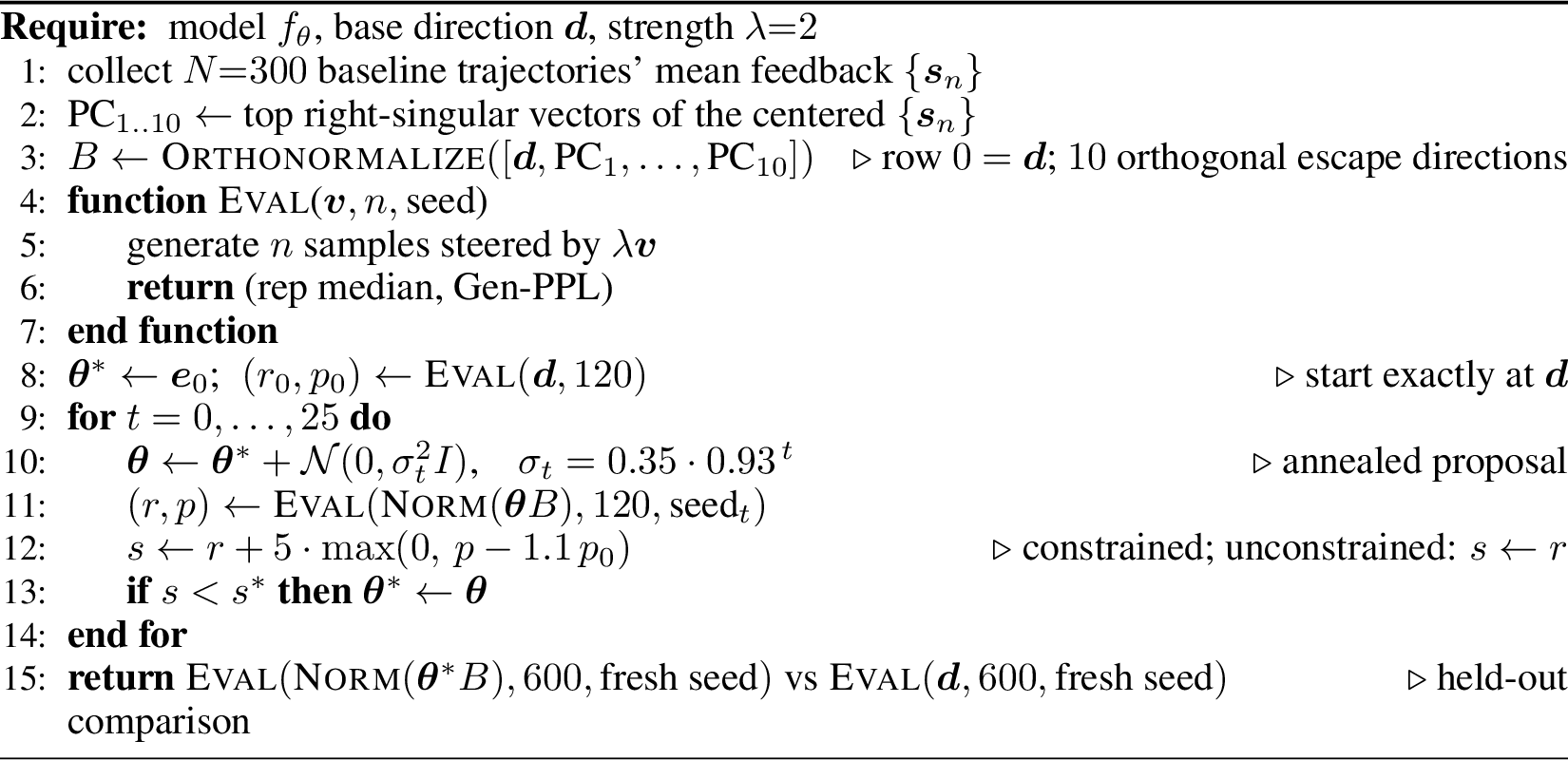
The alternatives above are cheap heuristics (full sweep in Tab. 5); we also ask whether any direction does better by optimizing the deployment objective itself (Algorithm 7). Steering leverage lives where the feedback varies, so the search space is the span of \(\boldsymbol{d}\) and the feedback’s top principal components, starting exactly at \(\boldsymbol{d}\). The constrained objective’s hinge penalty is a quality guard that fires only when a candidate degrades Gen-PPL more than \(10\%\) past the \(\boldsymbol{d}\) reference; PPL is never minimized, since under our thesis minimizing Gen-PPL would walk into the attractor.
9.1.0.2 \(\boldsymbol{d}\) is near-optimal.
An extensive search (up to \(30\) seeds across the two objectives) confirms direct optimization lowers repetition only slightly further than \(\boldsymbol{d}\), along essentially the same axis. On held-out seeds disjoint from the search (\(n{=}600\)), the constrained objective (minimize repetition subject to an on-manifold/Gen-PPL constraint) edges \(\boldsymbol{d}\) on repetition (median held-out \(1.85\%\) vs \(2.11\%\), winning \(24/30\) seeds) at matched Gen-PPL (\(27.7\) vs \(27.4\)). The unconstrained objective (minimize repetition alone, \(15\) seeds) lowers it a touch more (median \(1.84\%\), winning \(13/15\) seeds) at slightly worse Gen-PPL (\(28.1\)), while staying aligned with \(\boldsymbol{d}\) (median \(\cos{=}0.91\)): it trades a little quality for a small gain along essentially the same axis. The basin is thus approximately one-dimensional: a single cheap, label-free difference-of-means estimate captures it nearly as well as a direct optimization costing \({\sim}8\times\) the generations (\(3120\) vs \(400\)).
| Direction (objective) | rep % \(\downarrow\) | Gen-PPL \(\downarrow\) | Wins vs \(\bm{d}\) | generations | \(\cos\) to \(\bm{d}\) |
|---|---|---|---|---|---|
| Difference-of-means \(\bm{d}\) (ours) | \(2.11\) | \(27.4\) | – | \(\mathbf{400}\) | \(1.00\) |
| Constrained (min rep s.t.PPL) | \(1.85\) | \(27.7\) | 24/30 | \(3120\) | \(0.92\) |
| Unconstrained (min rep only, \(15\) seeds) | \(\mathbf{1.84}\) | \(28.1\) | 13/15 | \(3120\) | \(0.91\) |
| Property of \(\bm{d}\) at the operating point | Value |
|---|---|
| Aligned with the feedback’s leading PC, \(\lvert\cos(\bm{d},\mathrm{PC}_1)\rvert\) | \(0.73\) |
| Energy of \(\bm{d}\) in PC\(_1\) / top-\(5\) PCs | \(0.53\,/\,0.82\) |
| Estimate stable from few samples, \(\cos(\bm{d}_n,\bm{d}_{\text{full}})\) at \(n{=}50/200/800\) | \(0.69\,/\,0.94\,/\,1.00\) |
9.1.0.3 Seed-robustness.
The estimator comparison (Tab. 5) is reported at the \(\gamma{=}1.0\) operating point (§5), where difference-of-means recovers the most steerable direction: it beats the unsupervised top-PC, the Jacobian eigenvector (Tab. 9), and the logistic discriminant outright, and matches LDA. This is seed-robust: across three estimation seeds difference-of-means stays at or near the top (best in two, within \(0.6\) points of LDA in the third), while the top-PC and the Jacobian eigenvector remain far worse (\(\ge\!5\%\) steered rep) in every seed.
9.1.0.4 Data efficiency.
\(\boldsymbol{d}\) is cheap to estimate: the cosine between \(\boldsymbol{d}\) from \(n\) trajectories and the full-data direction reaches \(0.69\) at \(n{=}50\), \(0.94\) at \(n{=}200\), and \(1.00\) at \(n{=}800\). A few hundred unlabeled trajectories suffice, stable well before the repetition-tertile split matters.
9.1.0.5 Low-rank structure, one dominant self-amplified direction.
A PCA of the per-sample mean feedback (mean-centered over the \(n{=}1000\) samples; PC\(_1\) is its leading singular vector) concentrates the variance in a few components (PC\(_1\) explains \(18\%\), the top five \(46\%\)). The contraction makes \(\boldsymbol{v}_1\) a strong variance mode (propagating an isotropic initial spread through \(\boldsymbol{J}^k\) gives covariance \(\mathrm{Cov}(\boldsymbol{a}_k)=\sigma^2\boldsymbol{J}^{2k}=\sum_i\sigma^2\mu_i^{2k}\,\boldsymbol{v}_i\boldsymbol{v}_i^\top\), peaked on \(\boldsymbol{v}_1\)), so \(\boldsymbol{d}\) concentrates in the top components (\(53\%\) of \(\lVert\boldsymbol{d}\rVert^2\) in PC\(_1\), \(82\%\) in the top five, \(95\%\) in the top ten). But it is subdominant: the larger, sample-varying denoising variation pushes the raw top PC off \(\boldsymbol{v}_1\), so \(\lvert\cos(\boldsymbol{d},\text{PC}_1)\rvert{=}0.73\) rather than \(1\) and a plain PCA cannot cleanly isolate the axis. \(\boldsymbol{d}\) is instead the dominant self-amplification mode, the feedback Jacobian’s leading eigenvector (Tab. 9), which is why the unsupervised PC\(_1\) steers worse (Tab. 5).
9.1.0.6 When repetition emerges.
Repetition forms during the trajectory: how far a sample’s feedback drifts along \(\boldsymbol{d}\) predicts its final repetition (Fig. 2), the orbit being drawn into the attractor (Assumption 1). A cheap mid-trajectory check on the feedback can therefore flag doomed samples and reject or reset them early, complementing the steering fix that removes the pull at its source.
9.1.0.7 What \(\boldsymbol{d}\) encodes.
A linear logit-lens read of \(\boldsymbol{d}\) (projecting it through the output unembedding) ranks fragmentary subword pieces (tri, ction, iding, lect) among its top-scoring tokens and whole content words (emotion, scholarship, stretched) among its lowest: consistent with \(\boldsymbol{d}\) encoding the repetitive, sub-lexical loop content that steering removes.
10 Non-words and the steering window↩︎
10.1 Non-words: a second defect, independent of repetition↩︎
The non-word rate counts out-of-dictionary tokens [20]: length-\(\ge4\) alphabetic
tokens with zipf_frequency\(\,{=}\,0\) in wordfreq [21] (a
hunspell [22] cross-check preserves the ELF \(>\) human ordering). ELF generates them far above the
human floor, and Gen-PPL never sees them (Table 12).
| Generator | Params | non-word word % | non-word sample % |
|---|---|---|---|
| Human (BBC) | – | \(0.20\) | \(7.0\) |
| ELF-L-owt | \(652\)M | \(0.37\) | \(83.1\) |
| ELF-M-owt | \(342\)M | \(0.39\) | \(81.7\) |
| ELF-B-owt | \(105\)M | \(0.65\) | \(89.9\) |
| ELF-B-xsum | \(105\)M | \(1.09\) | \(18.5\) |
| ELF-B-de-en | \(105\)M | \(1.19^{\dagger}\) | \(18.7\) |
This is a decode-axis defect, statistically independent of the trajectory-axis repetition: a sample can be repetitive, non-word-laden, both, or neither. The decoder reads each latent position by an independent \(\arg\max\) at \(t{=}1\) with no autoregressive tie between neighbours, so individually legal word-pieces assemble into an illegal whole (glued non-words,
e.g.shock+d\(\to\)shockd). Because the two axes are independent, the self-conditioning fix targets repetition and not non-words; conversely, over-steering pushes the latent off the
embedding manifold and surfaces as a non-word spike (the \(\lambda_{\max}\) bound, Prop. 2), the signal that bounds the steering window from
above.
10.2 The steering \(\lambda\)-window↩︎
Two surface readouts bound the usable dose from opposite sides (Fig. 8). Lower edge: sweeping \(\lambda\) from \(0\), repetition falls steeply out of the basin from the closed-form threshold \(\lambda^\star{\approx}1.5\) (ELF-B crosses the human bar by \(\lambda{\approx}2.5\), the smaller models earlier). Upper edge: past it the latent leaves the embedding manifold and the non-word rate spikes (\(0.83\%\) at \(\lambda{=}6\) to \(2.42\%\) at \(\lambda{=}8\)), and repetition itself rebounds (back to \(5.03\%\) at \(\lambda{=}8\) from the \(1.11\%\) floor at \(\lambda{=}4\)): over-steering fails on both counts. The usable window is \(\lambda\in[1.5,5]\) and we operate at \(\lambda{=}2\).
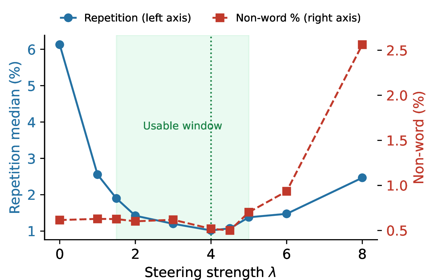
A single ELF-B direction \(\boldsymbol{d}_B\) at this one dose carries across sizes (Table 13): it tracks each size’s natively re-estimated direction throughout. \(\lambda{=}2\) is the knee of every size’s curve and the conservative operating point: it brings ELF-M and ELF-L well under the human bar and the hardest model ELF-B to just above it (\(2.11\%\) vs the \(1.92\%\) bar; \(\lambda{=}3\) takes ELF-B fully under, at \(1.37\%\)), while \(\lambda{=}4\) over-steers the larger two. One direction and one mild dose thus suffice across sizes.
| defect | quality | |||||
|---|---|---|---|---|---|---|
| 3-4(lr)5-7 Model | dose | rep % \(\downarrow\) | accept \(\uparrow\) | c-PPL \(\downarrow\) | dist-\(1\) \(\uparrow\) | s-BLEU \(\downarrow\) |
| ELF-B (\(105\)M) | base | \(6.83\) | \(0.07\) | \(27.7\) | \(0.53\) | \(0.09\) |
| \(1\) | \(3.32\) | \(0.27\) | \(28.8\) | \(0.55\) | \(0.10\) | |
| \(\mathbf{2}\) | \(2.11\) | \(0.45\) | \(30.6\) | \(0.53\) | \(0.15\) | |
| \(3\) | \(1.37\) | \(0.67\) | \(31.7\) | \(0.54\) | \(0.15\) | |
| \(4\) | \(1.11\) | \(0.77\) | \(30.6\) | \(0.52\) | \(0.18\) | |
| ELF-M (\(342\)M) | base | \(1.89\) | \(0.51\) | \(25.4\) | \(0.55\) | \(0.07\) |
| \(1\) | \(0.95\) | \(0.78\) | \(25.9\) | \(0.56\) | \(0.07\) | |
| \(\mathbf{2}\) | \(0.67\) | \(0.88\) | \(26.1\) | \(0.56\) | \(0.10\) | |
| \(3\) | \(0.55\) | \(0.93\) | \(27.0\) | \(0.56\) | \(0.11\) | |
| \(4\) | \(0.52\) | \(0.91\) | \(29.6\) | \(0.56\) | \(0.11\) | |
| ELF-L (\(652\)M) | base | \(1.66\) | \(0.56\) | \(26.2\) | \(0.56\) | \(0.07\) |
| \(1\) | \(0.98\) | \(0.77\) | \(27.4\) | \(0.58\) | \(0.08\) | |
| \(\mathbf{2}\) | \(0.71\) | \(0.84\) | \(28.5\) | \(0.58\) | \(0.10\) | |
| \(3\) | \(0.47\) | \(0.89\) | \(30.0\) | \(0.59\) | \(0.12\) | |
| \(4\) | \(0.39\) | \(0.92\) | \(31.3\) | \(0.59\) | \(0.14\) | |
5pt
11 Steering Pareto-dominates every soft self-conditioning alternative↩︎
11.0.0.1 The benchmarked alternatives (Tab. 14).
Each soft self-conditioning variant softens, rather than removes, the fed-back estimate \(\hat{\boldsymbol{x}}\) before it re-enters the loop, with no retraining. mag rescales it, \(\hat{\boldsymbol{x}}\!\gets\!\alpha\hat{\boldsymbol{x}}\), so \(\alpha{=}1\) is the unmodified full-SC sampler and \(\alpha{=}0\) is SC-reset (feedback disabled;
the \(\alpha\) sweep is Tab. 2). noise adds Gaussian noise, \(\hat{\boldsymbol{x}}\!\gets\!\hat{\boldsymbol{x}}+\sigma\boldsymbol{\epsilon}\), to break
the fixed point while keeping the signal. dist periodically decodes \(\hat{\boldsymbol{x}}\) to token logits and feeds back the temperature-weighted embedding \(\mathrm{softmax}(\text{logits}/T)\,\boldsymbol{E}\) (near-committed at small \(T\), mean-like at large \(T\)). cutoff turns self-conditioning off
entirely past a mid-trajectory step (feeding back \(\boldsymbol{0}\) thereafter); decay linearly anneals the feedback magnitude from full to a floor \(\alpha\) over the trajectory;
early-restart decodes \(\hat{\boldsymbol{x}}\) once mid-trajectory, flags the samples already repeating (token seq-rep-4 above a threshold), and resets their feedback to \(\boldsymbol{0}\) for the remaining steps. Full-SC (post-hoc reject) runs the unmodified sampler followed by the same reject-to-\(1000\) loop. ACE instead subtracts one direction, \(\hat{\boldsymbol{x}}\!\gets\!\hat{\boldsymbol{x}}-\lambda\boldsymbol{d}\) (§5), leaving the rest of the feedback intact. At the shared reject-to-\(1000\)
caliber, steering Pareto-dominates this frontier (§5; the full grid over every variant and both doses is Tab. 14); Fig. 9 gives the per-size cost of the
win.
| lower-rep dose | higher-rep dose | |||||
|---|---|---|---|---|---|---|
| 2-4(lr)5-7 Method | rep % | NFE | clean-PPL | rep % | NFE | clean-PPL |
| Human (reference) | \(0.00\) | – | \(14.4\) | reference | ||
| ACE, \(\lambda{=}2\) (ours) | \(2.11\) | \(144\) | \(30.3\) | our fix | ||
| hard SC (reset / Full-SC) | \(0.00\) | \(65\) | \(97.4\) | \(6.82\) | \(1040\) | \(27.6\) |
| soft-SC mag (\(\alpha{=}0.5/0.7\)) | \(1.94\) | \(138\) | \(34.5\) | \(4.56\) | \(416\) | \(29.1\) |
| soft-SC noise (\(\sigma{=}0.4/0.2\)) | \(5.06\) | \(630\) | \(29.8\) | \(6.15\) | \(997\) | \(27.8\) |
| soft-SC dist (\(T{=}1/2\)) | \(1.55\) | \(120\) | \(35.1\) | \(1.52\) | \(119\) | \(34.9\) |
| SC cutoff (\(\tau{=}0.3/0.5\)) | \(0.00\) | \(65\) | \(91.5\) | \(0.51\) | \(75\) | \(62.1\) |
| SC decay (\(1{\to}0\,/\,0.5\)) | \(1.96\) | \(140\) | \(38.5\) | \(5.96\) | \(593\) | \(28.7\) |
| SC early-restart (\(\tau{=}0.5/0.3\)) | \(1.05\) | \(97\) | \(54.9\) | \(3.56\) | \(173\) | \(74.3\) |
4pt

12 Building the fix into training (extended)↩︎
12.0.0.1 Setup.
We continue-train ELF-B from the released checkpoint on OpenWebText (fresh AdamW, weight decay \(0\), \(50\)-step warmup, effective batch \(512\), learning rate \(10^{-4}\), \(128\) optimizer steps), then evaluate the EMA weights by plain unsteered sampling on \(n{=}1000\) samples (rep: medians; clean-PPL: reject-to-\(1000\)), on the same footing as the released baseline. EMA decay is lowered from the release’s \(0.9999\) to \(0.999\) so the average tracks this short run. The continue-train control (\(w{=}0\)) and the anti-attractor regularizer (\(w{=}7\), best) of Table 3 share this recipe.
12.0.0.2 Anti-attractor regularization.
Rather than clean the feedback, teach the model not to produce attractor-direction feedback. Let \(\hat{\boldsymbol{x}}_\theta(\boldsymbol{z}_k,t_k)\in\mathbb{R}^{L\times e}\) be the model’s clean-latent prediction at noise level \(t_k\) and \(\boldsymbol{u}_\theta=\tfrac{1}{L}\sum_{l=1}^{L}\hat{\boldsymbol{x}}_\theta[l]\in\mathbb{R}^{e}\) its position-pooled estimate (the feedback \(\boldsymbol{u}\) of §4, equation 1 ). With the frozen difference-of-means direction \(\boldsymbol{d}\) (equation 8 ), the anti-attractor regularizer is \[\mathcal{L}_{\mathrm{attr}}(\theta)\;=\; \mathbb{E}_{\boldsymbol{z}_0,\,k}\!\left[\,\operatorname{ReLU}\!\big(\langle\boldsymbol{u}_\theta,\,\boldsymbol{d}\rangle\big)^{2}\,\right], \label{eq:attr}\tag{13}\] and we continue-train against \[\mathcal{L}(\theta)\;=\;\mathcal{L}_{\mathrm{base}}(\theta)\;+\;w\,\mathcal{L}_{\mathrm{attr}}(\theta), \qquad w\ge 0, \label{eq:trainobj}\tag{14}\] with \(\mathcal{L}_{\mathrm{base}}\) the standard flow-matching loss. The one-sided \(\operatorname{ReLU}\) is deliberate: only the \(+\boldsymbol{d}\) half-line is the repetitive basin (Prop. 2), so we penalize the model for pushing its own clean estimate toward the attractor while leaving the \(-\boldsymbol{d}\) side and all off-\(\boldsymbol{d}\) content \(\boldsymbol{w}\perp\boldsymbol{d}\) untouched. Because the penalty acts only on \(\hat{\boldsymbol{x}}_\theta\), the trained model needs no test-time intervention.
12.0.0.3 Result.
A short fine-tune (best at \(w{=}7\)) lowers plain repetition with coherent text at a small clean-PPL cost (Table 3); the same budget without the penalty (\(w{=}0\)) barely moves it, so the reduction is the regularizer’s, not the extra training. This confirms \(\boldsymbol{d}\) is a trainable, causal property, not just an inference-time handle.
13 Controls and example outputs↩︎
This appendix supports the causal test of §3 with the repetition–PPL association (§13.1), and collects example outputs: non-words (§13.2) and baseline-vs-steered repetition samples (§14).
13.1 Conditional PPL collapse (\(64\)-step operating point)↩︎
13.1.0.1 Association.
Table 15 stratifies the \(1{,}000\) samples of the \(64\)-step (\(\gamma{=}1.0\)) run by repetition; median GPT-2 PPL falls monotonically as repetition rises (Pearson \(r({\mathrm{\small rep}},{\mathrm{\small ppl}}){=}{-}0.63\), Spearman \(\rho{=}{-}0.68\)).
| rep range | \(n\) | median Gen-PPL |
|---|---|---|
| \(0{-}0.5\%\) | \(9\) | \(32.8\) |
| \(0.5{-}2\%\) | \(69\) | \(27.1\) |
| \(2{-}5\%\) | \(270\) | \(23.6\) |
| \(5{-}10\%\) | \(366\) | \(19.8\) |
| \(10{-}20\%\) | \(239\) | \(15.7\) |
| \(>20\%\) | \(47\) | \(10.3\) |
13.2 Example non-word outputs↩︎
All examples are from the ELF-B \(64\)-step (\(\gamma{=}1.0\)) run.
13.2.0.1 Non-words (with context).
The defect spans coinages, glued-together word pairs, and misspellings:
psychloginism: “The goal of psychloginism is to learn the…”intersignal: “…short of a bipartisan intersignal vote that would happen…”evenfigured: “…may occur and we’ve evenfigured out a way to…” (even + figured)slamed: “…his wife when he slamed a woman in the…” (slammed)encryptted: “…contains the first encryptted element…” (encrypted)
14 Qualitative samples: baseline vs.steered↩︎
14.0.0.1 Repetition emerging along the trajectory.
Decoding one sample’s current estimate at successive trajectory fractions shows the basin forming, the text counterpart of Figure 4. Table 16 shows one draw under baseline and steering at three trajectory stages: the baseline stays locked in the basin at \(38\)–\(45\%\) repeated \(4\)-grams, while the steered run stays near the human bar (\(1.0\)–\(3.1\%\)).
| Stage | Baseline (full-SC) | Steered (\(\lambda{=}2\)) | rep |
|---|---|---|---|
| early | When I spoke to my person. She said, “I don’t person’s life history, or does person’s life history? I mean, person’s life history. People asked person’s life history? I’s person’s life history? Interviewer – | In his speech to addressing the why the crisis said. "The crisis is completely and international officials have pressed | 22.5% \(\to\) 1.6% |
| mid | When I got out to person. She said, “I don’t person’s life history right or person’s life history? I mean, person’s life history – people person’s life history? And what person’s life history? Interviewer – | In his speech to on Thursday, on the crisis said. "The crisis is completely in Paris, where a unanimous and Palestinian officials have pushed | 27.8% \(\to\) 1.9% |
| final | Once I got to know person. She said, “I don’t person’s life history correct or person’s life history? I mean, person’s life history. But people person’s life history? And what person’s life history? Interviewer – | In his address to on Thursday,addressing the crisis in said. "The crisis is completely in Paris, where a joint and Palestinian officials have pushed | 26.8% \(\to\) 1.8% |
1pt
15 Related work↩︎
15.0.0.1 Diffusion-LM failure modes: metric and decoder.
Prior work on diffusion-LM failure modes mainly diagnoses evaluation artifacts or decoding bottlenecks, not text-visible repetition directly. The metric line shows generative perplexity is distorted by low-entropy or reduced-temperature sampling [8], [23], echoing broader evidence that model-based perplexity is unreliable for generation [9], [24] and gameable end-to-end by naive samplers [10]; this line is mostly on discrete or masked models. The decoder line targets per-position rounding and independence with stronger decoders [11], [12], [25], [26]: it addresses the discretization bottleneck, not the self-conditioning feedback direction behind text-visible repetition. An entropy view is in any case blind to whether the tokens are real words.
15.0.0.2 Reading the text, not the metric or the decoder.
We instead measure what the models generate, counting the defects a reader sees against human references. The closest prior model, the self-conditioned embedding diffusion of [27], reports likelihood/entropy trade-offs under guidance; relative to it and to the AR-repetition line [28], we study the generated text itself rather than a clean-embedding probe or the metric.
15.0.0.3 Relation to autoregressive degeneration.
Repetition is the denoising-axis analogue of classical AR-decoding degeneration [4]: the self-conditioning feedback plays the role of AR’s repeated-context prior and the low-entropy committed regime that of greedy maximization, but the errors compound along the denoising-step axis rather than the sequence-order axis. The correspondence is prescriptive: because repetition is set in the continuous latent, upstream of token selection, decode-time fixes such as contrastive search [15] are poorly placed to reach it, whereas the orthogonal non-word defect is amenable to AR-style contextual decoding (App. 10).
15.0.0.4 Relation to masked diffusion.
Two concurrent threads on masked diffusion bound our claims. [29] add self-conditioning to masked diffusion and report a large drop in generative perplexity without an explicit repetition analysis; whether masked, non-committed feedback enters the attractor we describe is left open. [13] steer a behavioral knob of masked DLMs (safety refusal) along an approximately one-dimensional subspace. A single-direction account of a DLM is thus not unique to us; what is specific here is a contractive attractor of the continuous self-conditioning loop, recovered label-free and targeting the generative-perplexity defect, captured by one frozen direction that generalizes across inference settings and model scales.
References↩︎
A generous bar; the few percent of human text above it is genuinely repetitive (lists, names, refrains).↩︎
No retraining: classifier-free guidance already trains the model both with the self-conditioning signal (\(\alpha{=}1\)) and without it (\(\alpha{=}0\)), so the sweep only interpolates between regimes it already runs.↩︎