Flow-Map GRPO: Reinforcement Learning for Few-Step Flow-Map Generators via Anchored Stochastic Composition
January 01, 1970
Abstract
Few-step flow-map generators, such as consistency models and MeanFlow, accelerate sampling by directly learning long-range transport maps between noise and data. However, these models are typically deterministic, which makes them difficult to optimize with reinforcement learning (RL) post-training methods that require stochastic trajectories and well-defined likelihood ratios. Existing SDE-based stochasticization techniques are designed for velocity-based samplers with infinitesimal or finely discretized transitions, and therefore do not directly apply to long-range flow maps. In this work, we propose Flow-Map GRPO, an online RL post-training framework for deterministic few-step flow-map generators. The key component is Anchored Stochastic Flow Map Composition (ASFMC), a path-preserving stochasticization mechanism that introduces randomness through anchor-based conditional resampling while preserving the original marginal probability path of the deterministic flow map. We derive GRPO objectives for both single-time and two-time flow-map parameterizations. Experiments on few-step FLUX-based text-to-image generators, including MeanFlow and sCM, show that Flow-Map GRPO improves pretrained deterministic flow-map models across reward-based, perceptual, and task-level evaluation metrics. Our results demonstrate that deterministic few-step flow-map generators can be effectively aligned with RL post-training without modifying their original model parameterization or retraining them as native stochastic models.
1 Introduction↩︎
Diffusion models and continuous-time flow-based generative models have become a dominant paradigm for high-quality image and video generation [1]–[3]. These methods construct a probability path between a simple prior distribution and the data distribution, and learn either a score field or a velocity field that defines a continuous-time generative process. In particular, flow-based approaches such as Flow Matching and Rectified Flow represent generation through a probability-flow ODE, which enables principled sampling by numerically integrating the learned velocity field. Despite their strong theoretical grounding, however, ODE-based sampling typically requires many discretization steps, leading to high computational cost at inference time.
This has motivated recent advances in few-step flow-map-based generative models, such as Consistency Models [4], [5] and MeanFlow [6]–[8]. Instead of learning only the instantaneous dynamics, these methods directly learn long-range mappings \(\psi_{t\to r}\) that map samples between two time points. By amortizing numerical integration into learned long-range mappings, flow-map-based models can replace iterative ODE solvers with one-step or few-step generation.
However, deterministic few-step flow maps pose a difficulty for RL post-training, which aims to align a pretrained generator with task-level rewards while preserving its original flow-map parameterization and learned marginal probability path. Recent reinforcement learning (RL) post-training methods for generative models, such as DDPO [9] and Flow-GRPO [10], formulate sampling as a Markov decision process and optimize the generative policy using task-level rewards. A key requirement of these methods is a well-defined stochastic transition kernel, which is needed both for trajectory-level exploration and for computing likelihood ratios in policy-gradient optimization. Diffusion models naturally provide such stochastic transitions through their denoising process, while velocity-based flow models can be equipped with stochastic transitions through path-preserving SDE reformulations [11]. In contrast, flow-map-based models directly parameterize deterministic long-range transports \(\psi_{t\to r}\), which do not define stochastic trajectories or transition likelihoods. This creates a structural mismatch between deterministic few-step flow-map generators and likelihood-ratio-based RL post-training methods [12].

A natural attempt is to introduce stochasticity by using a path-preserving SDE reformulation of the underlying ODE dynamics. While this works for velocity-based samplers with infinitesimal or finely discretized transitions, it does not directly extend to long-range flow maps. A long-range SDE transition depends on the entire stochastic path between the source and target times and, in general, cannot be reduced to a Gaussian transition centered at the deterministic flow-map output (see 1). Exact SDE-based stochasticization would therefore require stochastic integration, undermining the computational advantage of few-step flow maps. This motivates a stochasticization mechanism that operates directly at the level of flow maps while preserving their probability path.
To address this limitation, we propose Flow-Map GRPO, an online RL post-training framework for deterministic few-step flow-map generators. Its key component is Anchored Stochastic Flow Map Composition (ASFMC), a path-preserving stochasticization mechanism that introduces randomness at the level of long-range flow maps. Instead of perturbing infinitesimal dynamics, ASFMC uses an auxiliary anchor variable: given a deterministic transition from \(t\) to \(r\), it first maps the sample to the target time, transports this deterministic endpoint to an anchor time \(\tau\), and then resamples back to time \(r\) through a conditional transition of the probability path. In this way, the anchor connects deterministic flow-map composition with stochastic conditional resampling, producing stochastic transitions while preserving the marginal distribution learned by the original model. With ASFMC, each flow-map step becomes a stochastic policy transition, allowing few-step flow-map sampling to be formulated as an MDP and optimized with GRPO-style likelihood ratios. The construction is post-hoc and does not modify the pretrained flow-map parameterization. We instantiate it for both major flow-map forms: one-time endpoint maps, such as sCM, and two-time maps, such as MeanFlow, where ASFMC can use local or endpoint anchors. Our contributions are as follows:
We identify a fundamental limitation of SDE-based stochasticization for deterministic flow maps, showing that it is not directly applicable to long-range flow-map transitions.
We propose Anchored Stochastic Flow Map Composition (ASFMC), a principled stochastic flow-map construction that preserves the marginal probability path while enabling trajectory-level exploration.
We introduce Flow-Map GRPO, a unified RL post-training framework for deterministic few-step flow-map generators, and derive consistent formulations for both single-time and two-time flow-map parameterizations.
We empirically validate Flow-Map GRPO on few-step FLUX-based text-to-image generators, demonstrating improvements over pretrained MeanFlow and sCM checkpoints across reward-based, perceptual, and task-level evaluation metrics.
2 Background↩︎
2.1 Multi-Step Flow Models and Few-step Flow Maps↩︎
Let \(\mathcal{D}=\{x^i\in\mathcal{X}\}_{i=1}^n\) denote samples from an unknown data distribution \(p_1=p_{\mathrm{data}}\) on \(\mathcal{X}\subset\mathbb{R}^d\). A continuous-time generative model constructs a stochastic process \(\{X_t\}_{t\in[0,1]}\) whose marginal distribution \(p_t\) evolves from a simple base distribution \(p_0\), typically a standard Gaussian, to the data distribution \(p_1\), forming a probability path \(\{p_t\}_{t=0}^1\). The probability path can be described by a deterministic probability-flow ODE. Given an initial sample \(x_0\sim p_0\), its trajectory \(\{x_t\}_{t\in[0,1]}\) evolves according to \[\label{eq:ode} \frac{d x_t}{dt}=u_t(x_t), \qquad x_0\sim p_0 ,\tag{1}\] where \(u_t:\mathcal{X}\rightarrow\mathbb{R}^d\) is a time-dependent velocity field. The solution of 1 defines a time-dependent flow \(\psi_t:\mathcal{X}\rightarrow\mathcal{X}\) with \(\psi_0(x)=x\), such that \(x_t=\psi_t(x_0)\). \(\{X_t\}_{t\in[0,1]}\) is called a flow model [11] if it is generated by 1 , namely \(X_t=\psi_t(X_0)\), \(X_0\sim p_0\), and the corresponding marginal distribution can be induced by the pushforward \(p_t=[\psi_t]_\sharp p_0\), satisfying the continuity equation \[\label{eq:continuity} \partial_t p_t(x) = - \nabla\cdot(p_t(x)u_t(x)).\tag{2}\] Flow models cover major continuous-time generative models, including Flow Matching [13], Rectified Flow [14], and diffusion models such as DDIM [15].
Flow models learn \(u_t^\theta(x)\) (or an equivalent parameterization, such as epsilon prediction ) from \(\mathcal{D}\) and generate samples by numerically solving 1 . To train \(u_t^\theta(x)\), flow models construct conditional paths \(X_t=a_tX_1+b_tX_0\), where \(a_t\) and \(b_t\) are scheduler functions satisfying \(a_1=b_0=1\) and \(a_0=b_1=0\). The corresponding conditional velocity target is \(u_t(X_t| X_1,X_0)=\dot{a}_tX_1+\dot{b}_tX_0\). After marginalizing over \(X_0\), the conditional path and velocity become \(p_t(\cdot| X_1)\) and \(u_t(\cdot| X_1)\), whose marginalization again recovers the desired probability path and marginal velocity in 1 \(p_t(x)=\int p_t(x| x_1)p_1(x_1)dx_1\) and \(u_t(x)=\mathbb{E}[u_t(x| X_1)| X_t=x]\). For the affine conditional path above, the conditional velocity can be written as \[u_t(x| x_1) = \frac{\dot{b}_t}{b_t}x + ( \dot{a}_t-\frac{a_t\dot{b}_t}{b_t} )x_1,\] and the model is then trained with the surrogate objective \[\label{eq:objective} \mathcal{L}_c(\theta) = \mathbb{E}_{t,x_1\sim p_1,x\sim p_t(\cdot| x_1)} [ \|u_t^\theta(x)-u_t(x| x_1)\|^2 ]\tag{3}\] The Flow Matching and DDIM paths can be recovered by choosing \((a_t,b_t)=(t,1-t)\) and \((a_t,b_t)=(\sqrt{1-(1-t)^2},1-t)\), respectively. For conditional generation, the probability path and velocity field can be directly conditioned on \(c\) with \(p_t(x| x_1,c)\) and \(u_t(x|x_1,c)\).
The velocity field \(u^\theta_t\) only describes the instantaneous evolution of the generative process. After discretization, it gives a short-range transition from \(t\) to \(t+\Delta t\), so generating a sample requires repeatedly solving 1 over many steps. To enable one-step or few-step generation, flow-map-based methods, including Consistency Models [5] and MeanFlow [6], directly learn a flow map \(\psi^\theta_{t\to r}\), defined as \(\psi_{t\to r} = \psi_t\circ\psi^{-1}_t\), which enable one-step generation as \(x_1=\psi^\theta_{0\to 1}(x_0)\) and few-step generation, e.g., two step as \(x_{0.5}=\psi^\theta_{0\to 0.5}(x_0)\) and \(x_1=\psi^\theta_{0.5\to 1}(x_{0.5})\). Although flow-map-based methods have clear advantages in generation speed, they face a key training challenge that direct supervision for \(\psi_{t\to r}\) is difficult to obtain from the dataset [8]. In 7, we summarize common strategies for learning flow maps and discuss representative flow-map-based methods, including Consistency Models and MeanFlow.
2.2 Reinforcement Learning for Flow Models↩︎
Recent works [9], [10], [16], [17] aim to improve flow and diffusion models with task-specific rewards, such as human preference, aesthetic quality, or downstream evaluation metrics. These rewards are often non-differentiable; therefore, these methods formulate generation as a reinforcement learning problem by treating the sampling trajectory as a multi-step MDP. For a conditional generative model with condition \(c\), the state is \(s_t=(c,t,x_t)\), the action is the next sample along the trajectory, \(a_t=x_{t+\Delta t}\), and the policy is the model transition \(\pi_\theta(a_t| s_t)=p_\theta(x_{t+\Delta t}| x_t|c)\), the next-state transition is \(P(s_{t+\Delta t}| s_t,a_t) = \delta_{(c,t+\Delta t,a_t)}(s_{t+\Delta t})\). The initial state is drawn from \(\rho_0(s_0)=p(c)p_0(x_0)\), and the reward is assigned to the final generated sample, \(R(s_t,a_t)=r(x_1|c)\) when \(t=1\). The model can then be optimized with policy-gradient objectives based on the transition likelihood \(p_\theta(x_{t+\Delta t}| x_t|c)\).
The above formulation requires the policy \(\pi_\theta(a_t| s_t)=p_\theta(x_{t+\Delta t}| x_t|c)\) to be stochastic, so that the RL procedure can explore different trajectories and also the policy likelihood ratio \(\frac{\pi_\theta(a_t|s_t)}{\pi_{\theta_\text{ref}}(a_t|s_t)}\) used for regularization sometimes is well-defined rather than singular. DDPO [9] instantiates this framework for diffusion models. Since diffusion samplers, such as DDPM variants [18], naturally define stochastic denoising transitions, their transition likelihoods can be directly used for policy optimization. Flow-GRPO extends the same idea to flow models. Starting from the deterministic ODE in 1 , standard flow models do not directly provide stochastic actions or transition likelihoods for reinforcement learning. To introduce stochasticity, Flow-GRPO rewrites the deterministic flow dynamics as the following equivalent SDE [11]: \[\label{eq:flow95sde} dX_t=[u_t(X_t)+ \frac{\sigma_t^2}{2}\nabla_x \log p_t(X_t)]dt+\sigma_t dW_t,\tag{4}\] where \(\sigma_t\) controls the stochasticity and \(W_t\) denotes a standard Wiener process. The score correction cancels the diffusion effect at the marginal level, so the marginal path \(\{\tilde{p}_t\}_{t=0}^1\) induced by 4 matches the probability path \(\{p_t\}_{t=0}^1\) of the deterministic flow ODE in 1 , while retaining stochastic trajectories for GRPO exploration.
3 Method↩︎
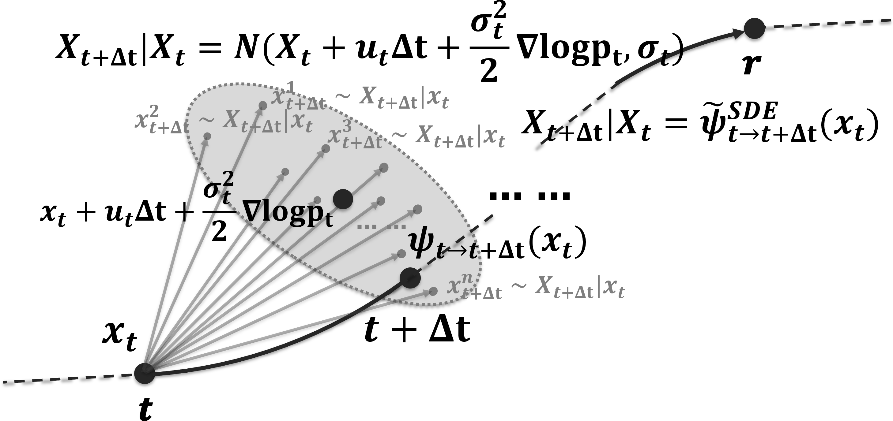
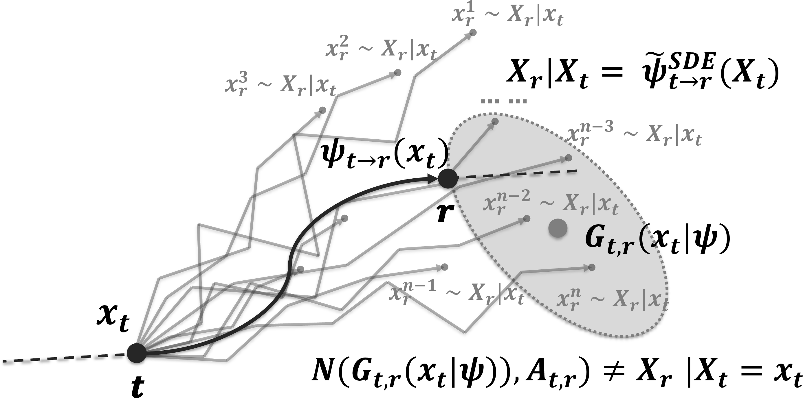
Figure 2: Comparison of SDE-induced stochasticization for infinitesimal and long-range transitions. For an infinitesimal transition \(\psi_{t\to t+\Delta t}\), the SDE corresponding to the deterministic ODE yields a simple Gaussian transition, enabling convenient stochasticization \({\tilde{\psi}}^{SDE}_{t\to t+\Delta t}\) of instantaneous velocity-based samplers. In contrast, for a long-range transition \(\psi_{t\to r}\), the accumulated stochastic dynamics generally cannot be reduced to a simple Gaussian form, preventing its direct use as a stochasticization mechanism \({\tilde{\psi}}^{SDE}_{t\to r}\) for flow maps.. a — Infinitesimal transition, b — Long-range transition
Existing RL post-training methods for generative models mainly target multi-step samplers, such as diffusion models [9] and flow matching models [10], where the generation process naturally forms a stochastic sequential decision process. In this work, we extend RL-based alignment to flow-map-based few-step generators [5], [6], [19]. A flow map defines a deterministic transport and therefore cannot be directly optimized with policy-gradient methods that require stochastic trajectories, and the key problem is how to introduce stochasticity into flow-map sampling without changing its underlying probability path, which becomes nontrivial due to the non-infinitesimal nature of flow-map dynamics (3.1). To address this problem, we propose Anchored Stochastic Flow Map Composition (ASFMC) method (3.2) and discuss how it can be instantiated for different flow-map parameterizations, including both two-parameter and one-parameter forms (3.3). Importantly, our method does not change the definition of the deterministic flow map, making it directly applicable to post-training existing flow-map models. We mainly instantiate our framework with GRPO [20], while noting that the same stochasticization principle can be combined with other RL algorithms and optimization techniques (4).
3.1 Challenge for Flow Maps↩︎
For RL post-training, the randomized flow map \(\tilde{\psi}_{t\to r}\) should satisfy two requirements. First, it should induce stochastic trajectories, allowing policy optimization to explore different generation paths. Second, it should preserve the original probability path of the pretrained flow map, so that the introduced stochasticity does not change the learned marginal distributions [10]. We formalize this requirement as follows.
Proposition 1 (Path-preserving stochasticization). Let \(\psi_{t\to r}\) denote a deterministic flow map that induces the probability path \(\{p_t = [\psi_{0\to t}]_\sharp p_0\}_{t=0}^1\). A valid randomized flow map \(\tilde{\psi}_{t\to r}\) for RL post-training should induce stochastic sample trajectories while preserving the same marginal path, i.e., its induced probability path \(\{\tilde{p}_t = [\tilde{\psi}_{0\to t}]_\sharp p_0\}_{t=0}^1\) satisfies \(\tilde{p}_t = p_t\) for all \(t\in[0,1]\).
A natural idea is to follow Flow-GRPO and inject stochasticity through an equivalent SDE whose marginal distributions match those of the deterministic ODE. For an infinitesimal step, the SDE induces a simple Gaussian transition \(x_{t+\Delta t} = x_t + [ u_t(x_t) + \frac{\sigma_t^2}{2}\nabla_x \log p_t(x_t) ]\Delta t + \sigma_t\sqrt{\Delta t}\epsilon_t\) with \(\epsilon_t\sim\mathcal{N}(0,I)\), which allows stochasticity to be conveniently injected into velocity-based samplers, as adopted by Flow-GRPO. However, flow maps are long-range transport operators between arbitrary time pairs, and their transitions are not infinitesimal. The long-range transition induced by the SDE generally cannot be reduced to a simple additive-noise form, i.e., a deterministic part plus an input-independent Gaussian perturbation, as shown in 2.
Theorem 2 (Long-range SDE transitions require stochastic integration). Let \(X_s\) solve the path-preserving SDE 4 and let \(\psi_{t\to r}\) be the deterministic flow map induced by the ODE 1 . For a non-infinitesimal interval \(t<r\), the exact SDE transition is generally not representable as a simple additive Gaussian perturbation of a deterministic function of the flow maps: \[X_r=G_{t,r}(X_t;\psi, d\psi,...)+ A_{t,r}\epsilon,\qquad \epsilon\sim\mathcal{N}(0,I),\] where \(A_{t,r}\) is independent of the input sample and \(G_{t,r}(X_t;\psi,d\psi,\ldots)\) denotes a deterministic functional of the flow-map family \(\psi\) and its derivatives. Instead, the exact transition must be expressed by the stochastic integral \(X_r=X_t+\int_t^r b_s(X_s)ds+\int_t^r \sigma_s dW_s\), where \(b_s(x) = u_s(x) + \frac{\sigma_s^2}{2}\nabla_x\log p_s(x)\), except for special linear-Gaussian dynamics. See 8.1 for proof.
As a result, the SDE-based stochasticization used in Flow-GRPO cannot be directly transferred to flow maps, which calls for a different stochasticization mechanism tailored to long-range flow-map transitions.
3.2 Anchored Stochastic Flow Map Composition↩︎
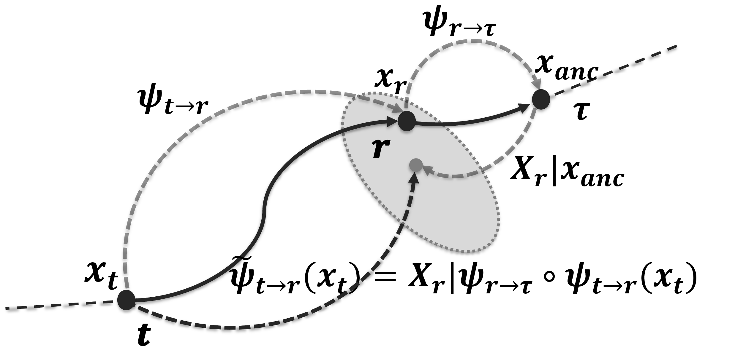
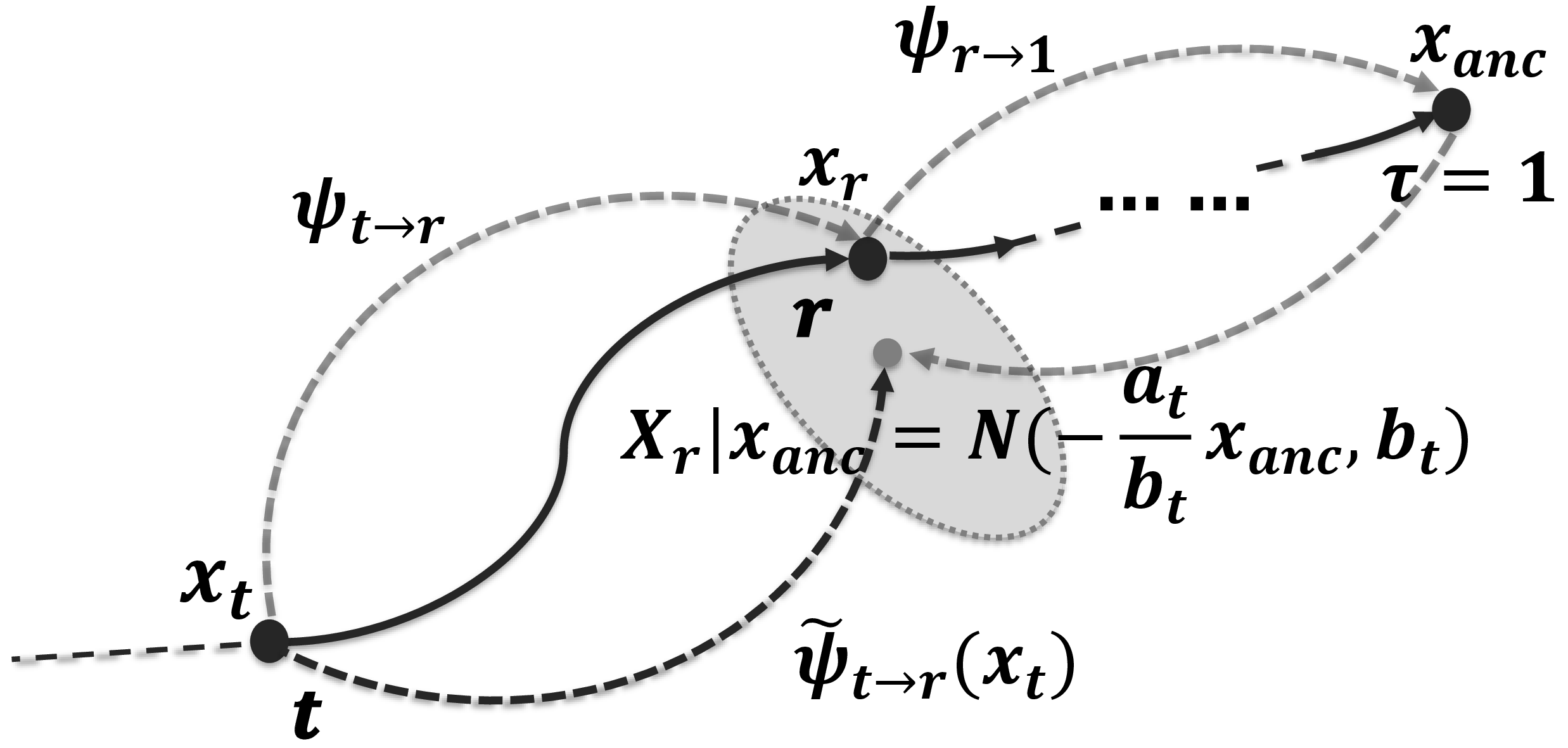
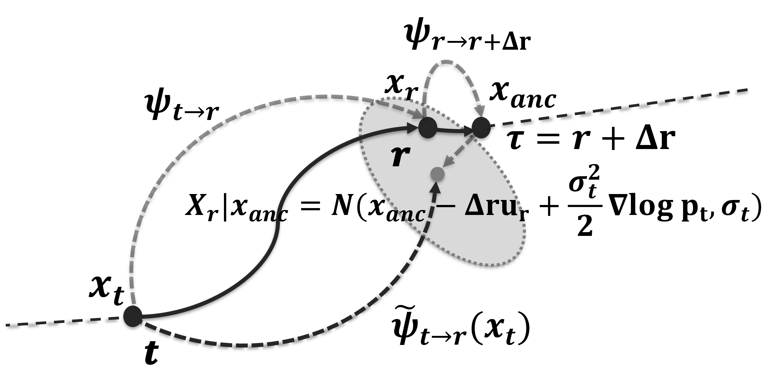
Figure 3: Illustration of Anchored Stochastic Flow Map Composition (ASFMC). Left: ASFMC decomposes a long-range transition \(\psi_{t\to r}\) into three flow-map segments, \(t\to r\), \(r\to \tau\), and \(\tau\to r\), with anchor time \(\tau\) and anchor state \(x_{\mathrm{anc}}\). The reverse segment \(r\to \tau\) samples a stochastic intermediate state conditioned on \(X_r\), thereby injecting randomness into the original transition \(t\to r\) while preserving the marginal path. Middle and right: two valid choices of the anchor time, \(\tau=1\) and \(\tau=r+\Delta r\) with small \(\Delta r\), respectively. We discuss another natural but invalid choice of \(\tau\) in 3.2.3.. a — ASFMC principle, b — Endpoint anchor, c — Local anchor
To address this challenge, we propose Anchored Stochastic Flow Map Composition (ASFMC), which injects randomness into flow-map sampling through an auxiliary anchor while preserving the original marginal path. The key intuition is that although the forward flow-map transition \(\psi_{t\to r}\) is deterministic, stochasticity can be introduced through a conditional transition, which is naturally stochastic, such as the noising or posterior transition in diffusion models. Specifically, ASFMC first moves the deterministic endpoint at time \(r\) to an anchor point \(x_{\mathrm{anc}}\) at the anchor time \(\tau\), and then samples back to time \(r\) through the conditional distribution \(p_{r| \tau}(\cdot| x_{\mathrm{anc}})\). The anchor \((\tau,x_{\mathrm{anc}})\) is therefore the shared interface between the deterministic compensation segment and the stochastic resampling segment, allowing ASFMC to combine flow-map composition with stochastic resampling while keeping the overall transition from \(t\) to \(r\) unchanged.
We now formalize the construction; see 3 (a) for an illustration. Given an input state \(x_t\) and a target time \(r\), the original deterministic flow map produces \(x_r = \psi_{t\to r}(x_t)\). ASFMC then chooses an anchor time \(\tau\) and defines the anchor state by transporting this deterministic endpoint to \(\tau\): \(x_{\mathrm{anc}} = \psi_{r\to \tau}(x_r) = \psi_{r\to \tau} \circ \psi_{t\to r}(x_t)\). The randomized output at time \(r\) is obtained by sampling from the conditional distribution back to the target time \(\tilde{x}_r \sim p_{r| \tau}(\cdot| x_{\mathrm{anc}})\). Namely, ASFMC defines the stochastic flow map \[\label{eq:anchor} \tilde{\psi}_{t\to r}(x_t) = \tilde{x}_r, \qquad \tilde{x}_r \sim p_{r| \tau} (\cdot | \psi_{r\to \tau} \circ \psi_{t\to r}(x_t) ).\tag{5}\] In this construction, the segment \(r\to\tau\) forms an anchor state with marginal \(p_\tau\), and the conditional transition \(\tau\to r\) injects randomness while returning to the target time. Thus, ASFMC preserves the original transition times and replaces the deterministic endpoint with a stochastic sample from the correct marginal. Moreover, this construction preserves the marginal distribution, since marginalizing the conditional transition \(p_{r| \tau}\) over the anchor marginal \(p_\tau\) recovers \(p_r\).
Theorem 3 (Path preservation of ASFMC). Let \(X_t\sim p_t\) and define \(X_r = \psi_{t\to r}(X_t)\), \(X_{\mathrm{anc}} = \psi_{r\to \tau}(X_r)\). If the randomized output \(\tilde{X}_r\) is sampled from the reverse conditional distribution \[\tilde{X}_r \sim p_{r| \tau}( \cdot | X_{\mathrm{anc}} ),\] then \(\tilde{X}_r\sim p_r\). Therefore, the stochastic flow map \(\tilde{\psi}_{t\to r}\) induced by ASFMC preserves the marginal distribution of \(\psi_{t\to r}\).
We next discuss the choice of the anchor time \(\tau\), which leads to different stochastic flow maps \(\tilde{\psi}_{t\to r}\). We consider three choices that are useful in different settings: a local anchor \(\tau=r+\Delta r\) with small \(\Delta r\), an endpoint anchor \(\tau=1\), and an intermediate anchor \(r<\tau<1\).

3.2.1 Local Anchor↩︎
The local anchor chooses an anchor time close to the target time, \(\tau=r+\Delta r\), where \(\Delta r>0\) is small. For the short anchor interval \([r,r+\Delta r]\), the conditional transition \(p_{r|r+\Delta r}\) can be approximated by the closed-form local Gaussian transition induced by the SDE corresponding to the reverse direction of the ODE in 1 from \(t=1\) to \(t=0\), while preserving the marginal path of the reverse-time dynamics: \(dX_t=[u_t(X_t)-\frac{\sigma_t^2}{2}\nabla_x\log p_t(X_t)]dt+\sigma_t dW_t\).We use the diffusion scale \(\sigma_r=\lambda\sqrt{\frac{2b_r(\dot{a}_r b_r - a_r \dot{b}_r)}{a_r}}\) following [10]. For a small step \(\Delta r>0\), the local transition from \(\tau\) to \(r\) takes the form by discretization \[\begin{align} \tilde{X}_r &= X_\tau - \Delta r [ u_\tau(X_\tau) - \frac{\sigma_\tau^2}{2}\nabla_x\log p_\tau(X_\tau)] + \sigma_\tau\sqrt{\Delta r}\xi + O(\Delta r^{3/2})\\ &= (1\!-\!\frac{\Delta r\sigma_\tau^2}{2}\frac{\dot{a}_r}{b_r(\dot{a}_r b_r - a_r \dot{b}_r)})X_\tau \!-\! \Delta r(1-\frac{\sigma_\tau^2}{2}\frac{a_r}{b_r(\dot{a}_r b_r - a_r \dot{b}_r)}) u_\tau(X_\tau) \!+\! \sigma_\tau\sqrt{\Delta r}\xi \!+\! O(\Delta r^{3/2})\\ &= (1-\frac{\lambda^2\Delta r\dot{a}_\tau}{a_\tau})X_\tau - \Delta r(1-\lambda^2) u_\tau(X_\tau) + \sigma_\tau\sqrt{\Delta r}\xi + O(\Delta r^{3/2})\\ \end{align}\] where \(\xi\sim\mathcal{N}(0,I)\), and \(\nabla_x\log p_r(X_r)=\frac{a_ru_r(X_r)-\dot{a}_rX_r}{b_r(\dot{a}_r b_r - a_r \dot{b}_r)}\) is the score function of the affine probability path. For the short forward deterministic segment \(r\to\tau\), we have \(X_\tau=\psi_{r\to r+\Delta r}(X_r)=X_r+\Delta r u_r(X_r)+O(\Delta r^2)\) by discretizing 1 . Substituting the above expressions for the deterministic segment \(r\to\tau\) and the stochastic segment \(\tau\to r\) into 5 and using the local approximations \(u_\tau(X_\tau)\approx u_r(X_r)\) and \(\sigma_\tau\approx\sigma_r\), we obtain the local-anchor stochastic flow map \[\tilde{\psi}_{t\to r}^{\mathrm{loc}}(X_t) = X_r-\Delta r\lambda^2[\frac{\dot{a}_\tau}{a_\tau}X_r-u_r(X_r)]+\sigma_\tau\sqrt{\Delta r}\xi+O(\Delta r^{3/2}), \qquad \xi\sim\mathcal{N}(0,I). \label{eq:local95anchor95update}\tag{6}\] This gives a simple closed-form stochasticization \(\tilde{\psi}_{t\to r}\) of the deterministic flow-map transition \(\psi_{t\to r}\), and the randomness is controlled by \(\sigma_\tau\sqrt{\Delta r}\). The following theorem proves the \(O((\Delta r)^{3/2})\) error bound for the approximation used in the above local-anchor derivation.
Theorem 4 (Error of the local-anchor approximation). Let \(\tilde{X}_r^\star\) denote the exact sample obtained by running the reverse-time SDE transition \(p_{r| \tau}(\cdot| X_\tau)\) from \(\tau=r+\Delta r\) to \(r\), where \(X_r=\psi_{t\to r}(X_t)\) and \(X_\tau=\psi_{r\to r+\Delta r}(X_r)\). Let \(\tilde{X}_r^{\mathrm{loc}}\) denote the local-anchor approximation \(\tilde{X}_r^{\mathrm{loc}} = X_r - \Delta r\lambda^2[ \frac{\dot{a}_r}{a_r}X_r-u_r(X_r)] + \sigma_r\sqrt{\Delta r}\xi\), \(\xi\sim\mathcal{N}(0,I)\), where \(\sigma_r=\lambda\sqrt{\frac{2b_r(\dot{a}_r b_r-a_r\dot{b}_r)}{a_r}}\). Assume that \(u_s(x)\), \(a_s\), \(b_s\), and \(\sigma_s\) are smooth with bounded derivatives in a neighborhood of the trajectory. Then the local-anchor approximation satisfies the strong error bound \[\|\tilde{X}_r^\star - \tilde{X}_r^{\mathrm{loc}}\|_{L^2}= O((\Delta r)^{3/2}).\] See 8.2 for the proof.
3.2.2 Endpoint Anchor↩︎
The endpoint anchor chooses \(\tau=1\). In this case, the anchor state is obtained by transporting the deterministic endpoint to the data endpoint: \(X_1=\psi_{r\to 1}(X_r)=\) \(X_r=\psi_{t\to r}(X_t)\). For the affine probability path, we have \(X_r=a_rX_1+b_rX_0\), where \(X_0\sim\mathcal{N}(0,I)\) is independent of \(X_1\). Therefore, the conditional distribution \(p_{r| 1}\) has the closed-form Gaussian expression \[p_{r| 1}(\cdot| X_1) = \mathcal{N}(a_rX_1,b_r^2 I).\] Thus, the endpoint-anchor stochastic flow map is given by \[\tilde{\psi}_{t\to r}^{\mathrm{end}}(X_t) = \tilde{X}_r = a_rX_1+b_r\xi = a_r\psi_{r\to 1}\circ\psi_{t\to r}(X_t)+b_r\xi, \qquad \xi\sim\mathcal{N}(0,I). \label{eq:endpoint95anchor95update}\tag{7}\] This gives a simple stochasticization of \(\psi_{t\to r}\) through the endpoint anchor. Compared with the local anchor, the endpoint anchor performs resampling from the endpoint conditional distribution \(p_{r|1}\) rather than from a short local interval, and therefore typically injects stronger randomness. However, this choice relies on the accuracy of the long-range map \(\psi_{r\to 1}\). This requirement may be restrictive in practice, especially for two-time flow-map models such as MeanFlow, which parameterize general transitions \(\psi_{t\to r}\) but are not specifically optimized as dedicated endpoint maps \(\psi_{t\to 1}\).

3.2.3 Intermediate Anchor↩︎
More generally, we may choose an intermediate anchor time \(r<\tau<1\). A natural but incorrect idea is to mimic the endpoint anchor and use the affine path to construct a closed-form transition. Since \(X_\tau=a_\tau X_1+b_\tau X_0\) and \(X_r=a_r X_1+b_r X_0\), one may sample a fresh noise variable \(\xi\sim\mathcal{N}(0,I)\), estimate \(X_1\) by \(\hat{X}_1=\frac{X_\tau-b_\tau \xi}{a_\tau}\), and then form \[\tilde{\psi}_{t\to r}(X_t) = \tilde{X}_r^{\mathrm{naive}} = a_r\hat{X}_1+b_r\xi=\frac{a_r}{a_\tau}X_\tau+(b_r-\frac{a_r b_\tau}{a_\tau})\xi,\qquad\xi\sim\mathcal{N}(0,I).\] However, this approximation treats the noise variable \(X_0\) as an unconditional Gaussian even after conditioning on \(X_\tau\). Indeed, the exact conditional distribution should sample \(X_0\) from its posterior given \(X_\tau\): \(p_{0| \tau}(x_0| x_\tau) \propto p_0(x_0) p_1 ( \frac{x_\tau-b_\tau x_0}{a_\tau} )\), up to the constant Jacobian factor. Therefore, the exact conditional transition is \[X_r| X_\tau = \frac{a_r}{a_\tau}X_\tau + ( b_r-\frac{a_r b_\tau}{a_\tau} )X_0, \qquad X_0\sim p_{0| \tau}(\cdot| X_\tau).\] Equivalently, \(p_{r| \tau}(x_r| x_\tau) = \int \delta (x_r-\frac{a_r}{a_\tau}x_\tau-( b_r-\frac{a_r b_\tau}{a_\tau} )x_0) p_{0| \tau}(x_0| x_\tau)dx_0\). The naive Gaussian formula above replaces \(p_{0| \tau}(\cdot| X_\tau)\) with the unconditional prior \(p_0=\mathcal{N}(0,I)\), thereby ignoring the posterior constraint imposed by the anchor state. This missing posterior correction can be substantial for intermediate anchors, because \(X_\tau\) contains information about both the data variable \(X_1\) and the noise variable \(X_0\). In our experiments, this approximation leads to large errors and unstable RL post-training.
3.3 Flow-Map GRPO↩︎
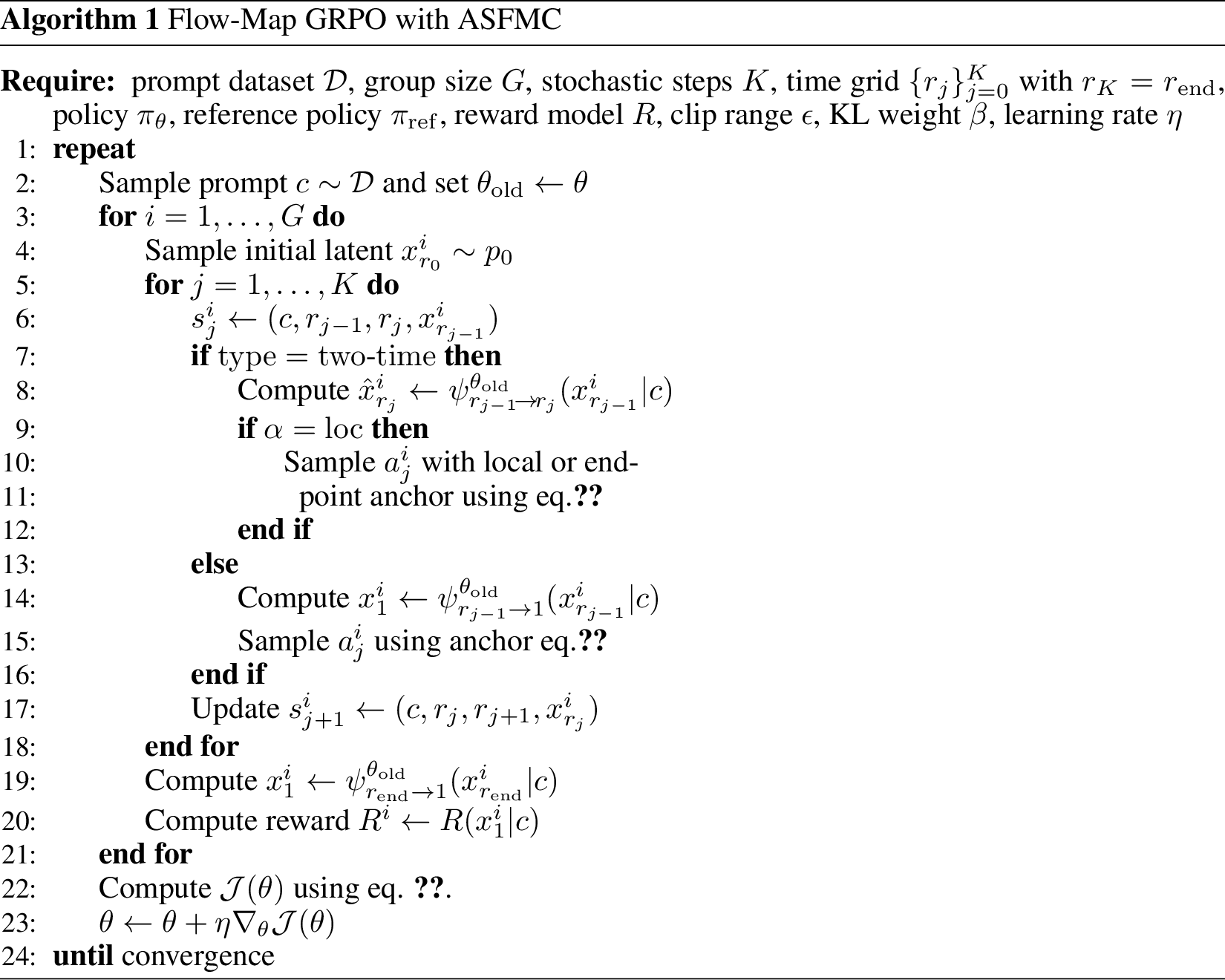
With ASFMC, a deterministic flow map is converted into a stochastic policy while preserving the original probability path. For a flow-map step from \(t_j\) to \(r_j\), we define the state as \(s_j=(c,t_j,r_j,x_{t_j})\) and the action as the next latent state \(a_j=x_{r_j}\). The policy is induced by the stochastic flow map \(\pi_\theta(a_j| s_j)= p_\theta(x_{r_j}| x_{t_j},c)=p_\theta(a_j=\tilde{\psi}_{t_j\to r_j}^{\theta}(x_{t_j}|c)|s_j)\). Given the sampled action \(a_j=x_{r_j}\), the MDP transition is deterministic \(P(s_{j+1}| s_j,a_j)=\delta_{(c,r_j,r_{j+1},a_j)}(s_{j+1})\), where the next state uses the sampled latent \(a_j\) as its input state. Therefore, ASFMC turns flow-map sampling into a stochastic multi-step MDP as in 2.2, enabling policy-gradient post-training. In this work, we instantiate the RL objective with GRPO, while noting that ASFMC is a stochasticization mechanism and can be combined with other RL algorithms.
Flow-map models can be broadly divided into two categories. Single-time flow maps learn a fixed endpoint map \(\psi_{t\to 1}\), while two-time flow maps directly learn transitions \(\psi_{t\to r}\) between arbitrary time pairs. We summarize these parameterizations in 7.2. We next discuss how to apply Flow-Map GRPO to these two settings.
3.3.1 Two-Time Flow Maps↩︎
Two-time flow maps can be naturally combined with both the local anchor and the endpoint anchor. We take MeanFlow [6] as an example, which parameterizes the transition by an average velocity \(u^\theta_{t\to r}\):\(\psi^\theta_{t\to r}(x_t|c) = x_t+(r-t)u^\theta_{t\to r}(x_t|c)\). We split the interval \([0,1]\) into \(K+1\) segments. The last segment \([r_{\mathrm{end}},1]\) is kept deterministic and is not optimized during RL post-training, similar to Flow-GRPO. The remaining stochastic transitions are defined on \([0,r_{\mathrm{end}}]\). Specifically, we first define uniform reference points \(\hat{r}_i=\frac{i}{K}r_{\mathrm{end}}\) for \(i=0,\ldots,K\), and then optionally apply an exponential time shift \(r_i = r_{\mathrm{end}} \frac{\exp(\gamma i/K)-1}{\exp(\gamma)-1}\), \(i=0,\ldots,K\), where \(\gamma\) controls the concentration of time points.
For each stochastic segment \(r_{j-1}\to r_j\), we instantiate the policy density using the ASFMC-randomized flow map \(a_j=x_{r_j}\sim \pi_\theta(\cdot\mid s_j)=\tilde{\psi}^{\theta}_{r_{j-1}\to r_j}(x_{r_{j-1}}|c)\), which can be computed by either the local-anchor update in 6 or the endpoint-anchor update in 7 \[\label{eq:two95time95anchor} \begin{align} a_j^{loc} &= \hat{x}_{r_j}-\Delta r\lambda^2[\frac{\dot{a}_\tau}{a_\tau}\hat{x}_{r_j}-u^\theta_{r\to r}(\hat{x}_{r_j})]+\sigma_\tau\sqrt{\Delta r}\xi\\ a_j^{end} &= a_r\psi^\theta_{r\to 1}(\hat{x}_{r_j})+b_r\xi,\\ \end{align}\tag{8}\] where \(\xi\sim\mathcal{N}(0,I)\) and \(\hat{x}_{r_j} = (r_j-r_{j-1})u^{\theta}_{r_{j-1}\to r_j}(x_{r_{j-1}}|c)+x_{r_{j-1}}\). After the \(K\) stochastic policy steps, the final deterministic segment maps \(x_{r_{\mathrm{end}}}\) to the data endpoint \(x_1=\psi^\theta_{r_{\mathrm{end}}\to 1}(x_{r_{\mathrm{end}}}|c)\), and the reward is evaluated only at the final sample, \(R(x_1|c)\). Given a prompt \(c\), we sample a group of \(G\) trajectories \(\{\tau^i\}_{i=1}^G\) from the old policy \(\pi_{\theta_{\mathrm{old}}}\) and compute the group-normalized advantage \(\hat{A}^i = \frac{ R(x^i_1|c)-\operatorname{mean}({R(x^j_1|c)}_{j=1}^G)}{ \operatorname{std}({R(x^j_1|c)}_{j=1}^G)}\). We optimize the flow-map policy with the GRPO objective \[\label{eq:FM95GRPO} \begin{align} \mathcal{J}_{\text{FM-GRPO}}(\theta)&= \mathbb{E}_{c,{\tau^i}_{i=1}^G\sim \pi_{\theta_{\mathrm{old}}}}[\frac{1}{G} \sum_{i=1}^G\frac{1}{K}\sum_{j=1}^K( \min(\rho^i_j(\theta)\hat{A}^i, \operatorname{clip}(\rho^i_j(\theta),1-\epsilon,1+\epsilon)\hat{A}^i)\\ &\qquad\qquad\qquad\qquad- \beta D_{\mathrm{KL}} (\pi_\theta(\cdot\mid s^i_j)|\pi_{\mathrm{ref}}(\cdot\mid s^i_j)))], \end{align}\tag{9}\] where \(s^i_j=(c,r_{j-1},r_j,x^i_{r_{j-1}})\) and \(\rho^i_j(\theta)=\frac{\pi_\theta(x^i_{r_j}\mid s^i_j)}{\pi_{\theta_{\mathrm{old}}}(x^i_{r_j}\mid s^i_j)}\). The final deterministic segment \(r_{\mathrm{end}}\to 1\) is used only to obtain the reward sample and is excluded from the policy-ratio and KL terms.
3.3.2 One-Time Flow Maps↩︎
One-time flow maps learn a fixed endpoint map \(\psi^\theta_{t\to 1}\) rather than arbitrary transitions \(\psi^\theta_{t\to r}\). We take sCM as an example, where the model directly predicts the endpoint state \(X_1=\psi^\theta_{t\to 1}(X_t|c)\). Following the sCM time parameterization, we uniformly split the angular interval \([0,\pi/2]\) into \(K+1\) segments, and use the corresponding cosine time points \(\{r_j\}_{j=0}^{K+1}\). The first \(K\) segments are used as stochastic policy steps for RL post-training, while the last segment \([r_K,r_{K+1}]\) is kept deterministic and used only to obtain the final sample. The main difference from two-time flow maps is that one-time flow maps cannot directly use the local anchor, since the local anchor requires a short transition \(\psi_{r\to r+\Delta r}\) or the instantaneous velocity \(u_r\), which is not provided by a fixed-endpoint model.
Fortunately, the endpoint anchor is directly compatible with one-time flow maps. For each stochastic segment \(r_{j-1}\to r_j\), we first predict the endpoint state \(X_1=\psi^\theta_{r_{j-1}\to 1}(X_{r_{j-1}}|c)\), and then sample the next latent state from the affine conditional path: \[\label{eq:one95time95anchor} \begin{align} a_j^{end}&=a_{r_j}\psi^\theta_{r_{j-1}\to 1}(x_{r_{j-1}}|c)+b_{r_j}\xi,\\ \xi&\sim\mathcal{N}(0,I). \end{align}\tag{10}\] Thus, the policy density is \(p_\theta(x_{r_j}\mid x_{r_{j-1}}|c)=\mathcal{N}(a_{r_j}\psi^\theta_{r_{j-1}\to 1}(x_{r_{j-1}}|c), b_{r_j}^2I)\). Given the sampled action \(a_j=x_{r_j}\), the MDP transition remains deterministic as before: \(P(s_{j+1}\mid s_j,a_j)=\delta_{(c,r_j,r_{j+1},a_j)}(s_{j+1})\). After the \(K\) stochastic endpoint-anchor steps, we use the deterministic endpoint map to obtain the final sample \(x_1=\psi^\theta_{r_{\mathrm{end}}\to 1}(x_{r_{\mathrm{end}}}|c)\), and evaluate the reward \(R(x_1|c)\). The GRPO objective is the same as in the two-time case, with the policy ratio computed using the one-time endpoint-anchor policy density above.
The detailed algorithm for 3.3.1 and 3.3.2 is given in Algorithm ¿tbl:alg:flowmap95grpo?. This algorithm enables GRPO post-training of flow-map-based few-step generators and can be combined with existing GRPO variants such as MixGRPO. During inference, the sampling procedure follows the standard one-time and two-time flow-map samplers, and we summarize these two sampling parameterizations in Algorithm ¿tbl:alg:flowmap95sampling?.
4 Experiment↩︎
4.1 Text-to-Image Generation↩︎
r0.52
We first evaluate Flow-Map GRPO for text-to-image post-training using the official T2I-Distill checkpoints released by [21], which are distilled from FLUX.1-lite and include both MeanFlow and sCM few-step generators. Starting from these pretrained flow-map models, we freeze the base generator and train only LoRA adapters. For each backbone, we perform reward-specific post-training with PickScore, OCR accuracy, and GenEval as the final-image reward, respectively. Each reward defines a separate training run and produces a separate LoRA adapter; across these runs, we keep the resolution, guidance scale, optimizer, LoRA architecture, rollout group size, and ASFMC stochasticization hyperparameters fixed. Thus, the only changes across the PickScore, OCR, and GenEval runs are the reward function and the corresponding prompt set. Details are shown in 9.1.
During RL post-training, all models use \(K=4\) stochastic ASFMC transitions. The reward is computed only from the final decoded image, while the likelihood-ratio and KL terms are evaluated on the \(K\) stochastic policy transitions. The final deterministic endpoint transition is used only to obtain the reward sample and is excluded from the policy-ratio and KL terms. At evaluation time, we follow the standard deterministic sampling procedure of each flow-map parameterization, as summarized in 7.2.
We report task-level, perceptual, and preference-based metrics, including GenEval, OCR accuracy, PickScore, aesthetic score, DQA, ImageReward, and UniReward, following [10]. Since MeanFlow and sCM use different flow-map parameterizations and native sampling schedules, we present their results in separate tables: MeanFlow results are shown in 1, 2, and 3, while sCM results are shown in 4, 5, and 6. Within each table, results are grouped by the number of inference steps. Flow-Map GRPO LoRA post-training is performed with \(K=4\), while evaluation is reported across multiple sampling steps to assess generalization across inference step counts. For each sampling budget, the pretrained base checkpoint and its Flow-Map GRPO LoRA counterpart are evaluated with the same sampler, inference schedule, guidance scale, resolution, and random seed. This isolates the effect of RL post-training within each flow-map parameterization. Additional qualitative comparisons are provided in 10.
| K | Model | Task Metrics | DrawBench Metrics | |||||||
|---|---|---|---|---|---|---|---|---|---|---|
| 3-5 (lr)6-11 | GenEval\(\uparrow\) | OCR Acc.\(\uparrow\) | PickScore Task\(\uparrow\) | DB-PickScore\(\uparrow\) | Aesthetic\(\uparrow\) | DeQA\(\uparrow\) | ImgRwd\(\uparrow\) | UniRwd\(\uparrow\) | DB Avg\(\uparrow\) | |
| 2 | MeanFlow Base | – | 0.2704 | – | 21.2756 | 5.3766 | 3.8431 | 0.1884 | 0.4931 | 31.1769 |
| MeanFlow + Flow-Map GRPO LoRA | – | 0.7404 | – | 21.2036 | 4.9996 | 3.0576 | -0.0145 | 0.4804 | 29.7266 | |
| 3 | MeanFlow Base | – | 0.3081 | – | 21.5679 | 5.5148 | 4.0511 | 0.3482 | 0.5338 | 32.0158 |
| MeanFlow + Flow-Map GRPO LoRA | – | 0.8477 | – | 21.6494 | 5.2110 | 3.5126 | 0.2763 | 0.5308 | 31.1801 | |
| 4 | MeanFlow Base | – | 0.3698 | – | 21.7724 | 5.5561 | 4.1318 | 0.4710 | 0.5551 | 32.4864 |
| MeanFlow + Flow-Map GRPO LoRA | – | 0.8815 | – | 21.9126 | 5.3086 | 3.7527 | 0.4334 | 0.5595 | 31.9668 | |
| 7 | MeanFlow Base | – | 0.4667 | – | 22.1137 | 5.6304 | 4.2106 | 0.6016 | 0.5873 | 33.1437 |
| MeanFlow + Flow-Map GRPO LoRA | – | 0.9154 | – | 22.2798 | 5.4462 | 4.0441 | 0.6696 | 0.6084 | 33.0481 | |
| 15 | MeanFlow Base | – | 0.5339 | – | 22.2734 | 5.6611 | 4.2425 | 0.7030 | 0.6078 | 33.4879 |
| MeanFlow + Flow-Map GRPO LoRA | – | 0.9288 | – | 22.4172 | 5.4708 | 4.1558 | 0.7579 | 0.6199 | 33.4217 | |
| K | Model | Task Metrics | DrawBench Metrics | |||||||
|---|---|---|---|---|---|---|---|---|---|---|
| 3-5 (lr)6-11 | GenEval\(\uparrow\) | OCR Acc.\(\uparrow\) | PickScore Task\(\uparrow\) | DB-PickScore\(\uparrow\) | Aesthetic\(\uparrow\) | DeQA\(\uparrow\) | ImgRwd\(\uparrow\) | UniRwd\(\uparrow\) | DB Avg\(\uparrow\) | |
| 2 | MeanFlow Base | – | – | 20.5865 | 21.2756 | 5.3766 | 3.8431 | 0.1884 | 0.4936 | 31.1774 |
| MeanFlow + Flow-Map GRPO LoRA | – | – | 22.5396 | 22.9231 | 5.7641 | 3.6197 | 1.1055 | 0.5977 | 34.0101 | |
| 3 | MeanFlow Base | – | – | 20.8831 | 21.5679 | 5.5148 | 4.0511 | 0.3482 | 0.5338 | 32.0157 |
| MeanFlow + Flow-Map GRPO LoRA | – | – | 23.0108 | 23.4095 | 5.9767 | 3.9998 | 1.2127 | 0.6455 | 35.2442 | |
| 4 | MeanFlow Base | – | – | 21.0952 | 21.7724 | 5.5561 | 4.1318 | 0.4710 | 0.5555 | 32.4868 |
| MeanFlow + Flow-Map GRPO LoRA | – | – | 23.2047 | 23.6309 | 6.0623 | 4.1365 | 1.2436 | 0.6655 | 35.7386 | |
| 7 | MeanFlow Base | – | – | 21.3676 | 22.1137 | 5.6304 | 4.2106 | 0.6016 | 0.5876 | 33.1440 |
| MeanFlow + Flow-Map GRPO LoRA | – | – | 23.4061 | 23.8306 | 6.1903 | 4.2691 | 1.2837 | 0.6826 | 36.2563 | |
| 15 | MeanFlow Base | – | – | 21.4136 | 22.2734 | 5.6611 | 4.2425 | 0.7030 | 0.6078 | 33.4879 |
| MeanFlow + Flow-Map GRPO LoRA | – | – | 23.4496 | 23.8891 | 6.2606 | 4.3341 | 1.3039 | 0.6892 | 36.4769 | |
3.5pt
| K | Model | Task Metrics | DrawBench Metrics | |||||||
|---|---|---|---|---|---|---|---|---|---|---|
| 3-5 (lr)6-11 | GenEval\(\uparrow\) | OCR Acc.\(\uparrow\) | PickScore Task\(\uparrow\) | DB-PickScore\(\uparrow\) | Aesthetic\(\uparrow\) | DeQA\(\uparrow\) | ImgRwd\(\uparrow\) | UniRwd\(\uparrow\) | DB Avg\(\uparrow\) | |
| 3 | MeanFlow Base | 0.4919 | – | – | 21.5679 | 5.5148 | 4.0511 | 0.3482 | 0.5338 | 32.0158 |
| MeanFlow + Flow-Map GRPO LoRA | 0.6330 | – | – | 20.9773 | 4.9029 | 2.5845 | -0.1520 | 0.4502 | 28.7628 | |
| 4 | MeanFlow Base | 0.5117 | – | – | 21.7724 | 5.5561 | 4.1318 | 0.4710 | 0.5551 | 32.4864 |
| MeanFlow + Flow-Map GRPO LoRA | 0.7315 | – | – | 21.4273 | 5.0450 | 3.0630 | 0.2152 | 0.5068 | 30.2574 | |
| 7 | MeanFlow Base | 0.5428 | – | – | 22.1137 | 5.6304 | 4.2106 | 0.6016 | 0.5873 | 33.1437 |
| MeanFlow + Flow-Map GRPO LoRA | 0.8113 | – | – | 21.8074 | 5.1332 | 3.5618 | 0.4990 | 0.5551 | 31.5566 | |
| 15 | MeanFlow Base | 0.5497 | – | – | 22.2734 | 5.6611 | 4.2425 | 0.7030 | 0.6078 | 33.4879 |
| MeanFlow + Flow-Map GRPO LoRA | 0.8409 | – | – | 21.9382 | 5.1779 | 3.7964 | 0.5704 | 0.5803 | 32.0632 | |
3.5pt
| K | Model | Task Metrics | DrawBench Metrics | |||||||
|---|---|---|---|---|---|---|---|---|---|---|
| 3-5 (lr)6-11 | GenEval\(\uparrow\) | OCR Acc.\(\uparrow\) | PickScore Task\(\uparrow\) | DB-PickScore\(\uparrow\) | Aesthetic\(\uparrow\) | DeQA\(\uparrow\) | ImgRwd\(\uparrow\) | UniRwd\(\uparrow\) | DB Avg\(\uparrow\) | |
| 2 | sCM Base | – | 0.3347 | – | 21.4096 | 5.3940 | 3.2930 | 0.5690 | 2.6314 | 33.2970 |
| sCM + Flow-Map GRPO LoRA | – | 0.8449 | – | 21.7509 | 5.1688 | 3.3645 | 0.3984 | 2.6761 | 33.3587 | |
| 3 | sCM Base | – | 0.4243 | – | 21.4594 | 5.4468 | 3.4805 | 0.5783 | 2.7145 | 33.6795 |
| sCM + Flow-Map GRPO LoRA | – | 0.9038 | – | 21.9248 | 5.2884 | 3.7097 | 0.4750 | 2.7878 | 34.1857 | |
| 4 | sCM Base | – | 0.4783 | – | 21.4914 | 5.4745 | 3.5734 | 0.5785 | 2.7046 | 33.8224 |
| sCM + Flow-Map GRPO LoRA | – | 0.9221 | – | 21.9349 | 5.3522 | 3.8697 | 0.5109 | 2.8652 | 34.5329 | |
| 7 | sCM Base | – | 0.6086 | – | 21.4984 | 5.5112 | 3.6908 | 0.6071 | 2.7467 | 34.0542 |
| sCM + Flow-Map GRPO LoRA | – | 0.9318 | – | 21.8895 | 5.4672 | 4.0625 | 0.5179 | 2.8546 | 34.7917 | |
| 15 | sCM Base | – | 0.6694 | – | 21.3812 | 5.5457 | 3.7325 | 0.5216 | 2.6981 | 33.8791 |
| sCM + Flow-Map GRPO LoRA | – | 0.9186 | – | 21.6972 | 5.4668 | 4.0658 | 0.4416 | 2.8257 | 34.4971 | |
3.5pt
| K | Model | Task Metrics | DrawBench Metrics | |||||||
|---|---|---|---|---|---|---|---|---|---|---|
| 3-5 (lr)6-11 | GenEval\(\uparrow\) | OCR Acc.\(\uparrow\) | PickScore Task\(\uparrow\) | DB-PickScore\(\uparrow\) | Aesthetic\(\uparrow\) | DeQA\(\uparrow\) | ImgRwd\(\uparrow\) | UniRwd\(\uparrow\) | DB Avg\(\uparrow\) | |
| 2 | sCM Base | – | – | 20.2924 | 21.4096 | 5.3940 | 3.2930 | 0.5690 | 2.6300 | 33.2956 |
| sCM + Flow-Map GRPO LoRA | – | – | 23.0733 | 23.4608 | 5.8943 | 3.8811 | 1.1759 | 3.1291 | 37.5412 | |
| 3 | sCM Base | – | – | 20.2841 | 21.4594 | 5.4468 | 3.4805 | 0.5783 | 2.7155 | 33.6805 |
| sCM + Flow-Map GRPO LoRA | – | – | 23.2256 | 23.6317 | 5.9099 | 4.0854 | 1.2126 | 3.2613 | 38.1009 | |
| 4 | sCM Base | – | – | 20.3520 | 21.4914 | 5.4745 | 3.5734 | 0.5785 | 2.7059 | 33.8237 |
| sCM + Flow-Map GRPO LoRA | – | – | 23.2781 | 23.6559 | 5.9057 | 4.1699 | 1.2092 | 3.2988 | 38.2395 | |
| 7 | sCM Base | – | – | 20.2870 | 21.4984 | 5.5112 | 3.6908 | 0.6071 | 2.7470 | 34.0545 |
| sCM + Flow-Map GRPO LoRA | – | – | 23.2254 | 23.6130 | 5.8814 | 4.2523 | 1.1777 | 3.3508 | 38.2752 | |
| 15 | sCM Base | – | – | 20.0630 | 21.3812 | 5.5457 | 3.7325 | 0.5216 | 2.6999 | 33.8809 |
| sCM + Flow-Map GRPO LoRA | – | – | 22.9545 | 23.3792 | 5.8529 | 4.2720 | 1.1069 | 3.2947 | 37.9057 | |
3.5pt
| K | Model | Task Metrics | DrawBench Metrics | |||||||
|---|---|---|---|---|---|---|---|---|---|---|
| 3-5 (lr)6-11 | GenEval\(\uparrow\) | OCR Acc.\(\uparrow\) | PickScore Task\(\uparrow\) | DB-PickScore\(\uparrow\) | Aesthetic\(\uparrow\) | DeQA\(\uparrow\) | ImgRwd\(\uparrow\) | UniRwd\(\uparrow\) | DB Avg\(\uparrow\) | |
| 2 | sCM Base | 0.5436 | – | – | 21.4096 | 5.3940 | 3.2930 | 0.5690 | 2.6290 | 33.2946 |
| sCM + Flow-Map GRPO LoRA | 0.8423 | – | – | 20.9817 | 4.9896 | 3.0097 | 0.0562 | 2.6094 | 31.6466 | |
| 3 | sCM Base | 0.5127 | – | – | 21.4594 | 5.4468 | 3.4805 | 0.5783 | 2.7148 | 33.6798 |
| sCM + Flow-Map GRPO LoRA | 0.8814 | – | – | 21.2339 | 5.0886 | 3.3370 | 0.2568 | 2.7611 | 32.6774 | |
| 4 | sCM Base | 0.5205 | – | – | 21.4914 | 5.4745 | 3.5734 | 0.5785 | 2.7073 | 33.8251 |
| sCM + Flow-Map GRPO LoRA | 0.8947 | – | – | 21.2995 | 5.1348 | 3.5168 | 0.3306 | 2.8204 | 33.1021 | |
| 7 | sCM Base | 0.4830 | – | – | 21.4984 | 5.5112 | 3.6908 | 0.6071 | 2.7480 | 34.0555 |
| sCM + Flow-Map GRPO LoRA | 0.9074 | – | – | 21.4316 | 5.1999 | 3.7408 | 0.4452 | 2.9215 | 33.7390 | |
| 15 | sCM Base | 0.4337 | – | – | 21.3812 | 5.5457 | 3.7325 | 0.5216 | 2.7001 | 33.8811 |
| sCM + Flow-Map GRPO LoRA | 0.9094 | – | – | 21.3911 | 5.1999 | 3.8372 | 0.4767 | 2.8975 | 33.8024 | |
3.5pt
5 Related Work↩︎
5.0.0.1 Continuous-time generative models.
Diffusion models and continuous-time flow-based models have become a central framework for high-quality generative modeling. Diffusion models define a stochastic noising process and learn to reverse it through denoising or score estimation [15], [18], [22]. In parallel, flow-based formulations such as flow matching and rectified flow learn a time-dependent velocity field that transports a simple prior distribution to the data distribution through a probability-flow ODE [13], [14]. Stochastic interpolants further provide a broad framework that connects deterministic flows and stochastic diffusions through probability paths [23]. These continuous-time models provide a principled foundation for generative sampling, but typically require many numerical integration steps at inference time.
5.0.0.2 Few-step flow-map generation.
To reduce sampling cost, recent methods learn long-range transport operators, or flow maps, that directly map samples between time points. Consistency models learn mappings from noisy states to clean data and enable one-step or few-step generation through self-consistency constraints [4], [5], [24]. Flow Map Matching provides a mathematical framework for learning two-time flow maps of an underlying probability-flow dynamics and connects flow maps with consistency models and progressive distillation [12]. Shortcut models and MeanFlow further parameterize long-range transitions or average velocities, allowing direct jumps over arbitrary time intervals and enabling efficient few-step generation [6], [7], [19]. These methods achieve fast inference by replacing iterative ODE integration with deterministic long-range mappings. However, because the learned transition \(\psi_{t\rightarrow r}\) is deterministic, these models do not naturally define stochastic trajectories or transition likelihoods, which makes direct reinforcement learning post-training nontrivial.
5.0.0.3 Reinforcement learning for generative models.
Reinforcement learning has recently been used to align generative models with task-level rewards, including human preference, aesthetic quality, and downstream evaluation metrics. DDPO formulates diffusion sampling as a multi-step Markov decision process and applies policy-gradient optimization to stochastic denoising trajectories [9]. Subsequent methods extend similar ideas to visual generation and flow-based models [10], [16], [17]. In particular, Flow-GRPO introduces stochasticity into velocity-based flow models by replacing the deterministic probability-flow ODE with a path-preserving SDE, thereby obtaining stochastic transitions and likelihood ratios for GRPO optimization. Relatedly, GLASS Flows [25] improve stochastic transition sampling for inference-time alignment of continuous-time flow and diffusion models. The main difference from our setting is that these methods target diffusion or velocity-based flow models, where generation is represented through infinitesimal or finely discretized transitions. In contrast, few-step flow-map models directly parameterize long-range transports \(\psi_{t\rightarrow r}\). For such transitions, the corresponding SDE-induced transition generally depends on the stochastic path between \(t\) and \(r\), and therefore cannot be treated as a simple local Gaussian perturbation of the deterministic flow map. As a result, stochasticization techniques developed for velocity-based samplers are not directly applicable to deterministic flow-map generators without an additional path-preserving construction.
5.0.0.4 Stochastic and reward-aware flow maps.
Several recent works have explored stochastic variants of flow maps for posterior sampling and reward alignment. Meta Flow Maps (MFMs) [26] extend consistency models and flow maps into the stochastic regime by training a model to perform one-step posterior sampling, producing multiple samples from \(p(x_1 \mid x_t)\) given an intermediate noisy state. Diamond Maps [27] propose stochastic flow-map models designed for efficient reward alignment, aiming to make adaptability to arbitrary rewards an intrinsic property of the generative model. Strong Stochastic Flow Maps [28] directly generalize deterministic flow maps to the stochastic setting by learning strong solution maps of additive-noise SDEs, while stochastic few-step models [29] study efficient few-step sampling from SDE-defined conditional distributions. Relatedly, Flow Map Reward Guidance [30] uses flow maps for training-free reward guidance from an optimal-control perspective.
These methods are closely related in that they also recognize the importance of stochasticity or reward-aware control for efficient alignment. However, they address a different regime from ours. Existing stochastic flow-map methods typically train or redesign the generative model to be stochastic by construction, for example by learning a native stochastic transition kernel, posterior sampler, or stochastic solution map. In contrast, our goal is to start from a pretrained deterministic flow map and introduce stochasticity only as a post-hoc transformation for RL post-training. Our ASFMC construction does not change the deterministic flow-map parameterization. Instead, it composes the deterministic flow map with anchor-based conditional resampling, yielding a path-preserving stochastic policy suitable for likelihood-ratio-based GRPO optimization.
5.0.0.5 Positioning.
Our work is complementary to native stochastic flow-map learning. Rather than training a new stochastic flow-map model class, we provide a stochasticization mechanism for existing deterministic few-step generators. This distinction is important for practical post-training: ASFMC allows pretrained consistency-style or MeanFlow-style models to be converted into stochastic policies without modifying their original training objective or model parameterization.
6 Conclusion↩︎
We presented Flow-Map GRPO, a reinforcement learning post-training framework for deterministic few-step flow-map generators. Our starting point is the observation that existing SDE-based stochasticization methods, although effective for velocity-based diffusion and flow models, are intrinsically local and do not directly extend to long-range flow-map transitions. To overcome this limitation, we introduced Anchored Stochastic Flow Map Composition , which converts a deterministic flow map into a stochastic policy by combining deterministic transport with anchor-based conditional resampling. This construction preserves the original marginal probability path while providing the trajectory-level stochasticity needed for policy-gradient optimization. Building on ASFMC, we formulated few-step flow-map sampling as a stochastic MDP and derived a GRPO-style objective that applies to both single-time and two-time flow-map parameterizations. Empirically, we validated our method on few-step FLUX-based text-to-image generators, showing that RL post-training can improve pretrained MeanFlow and sCM checkpoints across reward-based, perceptual, and task-level metrics.
Our work suggests that deterministic few-step generators can benefit from the same reward-driven post-training paradigm that has proven effective for diffusion and velocity-based flow models, provided that stochasticity is introduced in a way that respects the underlying probability path. We hope this opens a path toward broader RL alignment of fast generative models, including more general flow-map architectures and other few-step image, video, and multimodal generators.
Appendix↩︎
7 Flow-Map-Based Few-Step Method↩︎
7.1 Flow Map Learning↩︎
As discussed in 2.1, flow-map learning aims to directly learn the long-range transport map \(\psi_{t\to r}\) associated with an underlying probability flow. Once such a map is available, one-step generation can be performed by \(x_1 = \psi^\theta_{0\to 1}(x_0)\), \(x_0 \sim p_0\). This perspective differs from conventional multi-step generative modeling, which learns an instantaneous velocity \(u_t\) or score field \(\nabla \log p_t\) and then numerically integrates the corresponding dynamics. Flow-map learning instead attempts to amortize this integration into a mapping that performs a long-range transition in one or a few network evaluations.
A central difficulty is that there is usually no easily computable closed-form target flow map \(\psi_{t\to r}(x_t)\) for direct supervision. Therefore, one cannot simply train the model with a direct regression objective of the form \(|\psi^\theta_{t\to r}(x_t)-\psi_{t\to r}(x_t)|_2^2\). In multi-step methods such as Flow Matching, this issue is circumvented by constructing a conditional probability path \(p_t(x_t|x_1)\) and using an associated instantaneous quantity, such as the conditional velocity \(u_t(x_t|x_1)\), to regress the marginal velocity: \[\mathcal{L}_{\mathrm{FM}}(\theta) = \mathbb{E}_{t,\,x_1\sim p_1,\,x_t\sim p_{t|1}(\cdot|x_1)} [ \| u^\theta(x_t,t)-u_t(x_t|x_1) \|_2^2 ].\] The same strategy, however, does not directly extend to flow maps. Unlike instantaneous velocity fields, long-range flow maps do not admit a self-consistent conditional counterpart.
Theorem 5 ((Non-existence of conditional flow maps; Theorem 4.1 of [8])). There exists no conditional flow map \(\psi_{t\to r}(x|x_1)\) that simultaneously (1) is consistent with the conditional velocity \(u_t(x|x_1)\) under the flow-map evolution equation in 1 ; and (2) satisfies the marginal consistency relation \(\psi_{t\to r}(x)=\mathbb{E}_{x_1\sim p_t(x_1|x)}[\psi_{t\to r}(x|x_1)]\). Consequently, a self-consistent conditional cumulative field does not exist.
Because such a conditional flow map does not exist, flow-map learning is typically formulated through surrogate objectives based on trajectory consistency. In particular, the semigroup property of the exact flow map implies \[\psi_{t\to r}(x_t)=\psi_{s\to r}(\psi_{t\to s}(x_t)), \qquad t,s,r\in[0,1],\] which motivates the trajectory-consistency loss \(\mathcal{L}^{\mathrm{TC}}(\theta)=\mathbb{E}_{t,s,r,\,x_t\sim p_t} [\|\psi^\theta_{t\to r}(x_t)-\psi^\theta_{s\to r}(\psi^\theta_{t\to s}(x_t))\|_2^2]\). However, this loss alone does not provide dataset-level supervision: all terms are generated by the model itself. Therefore, \(\mathcal{L}^{\mathrm{TC}}\) can enforce internal consistency of the learned maps, but it cannot by itself guarantee that \(\psi^\theta_{0\to 1}\) pushes \(p_0\) to the desired target distribution \(p_1\).
Existing flow-map-based generative models can therefore be broadly organized into two categories according to how they obtain supervision for long-range maps: progressive distillation methods and derivative-based methods [8]. The former progressively transfers supervision from short-range transitions to longer-range maps, while the latter derives differential identities that connect long-range maps to instantaneous velocity or score fields. We first summarize these two families and then discuss two representative derivative-based models used in our experiments: sCM and MeanFlow.
7.1.0.1 Progressive distillation methods.
Progressive distillation methods learn short-range transitions first and then extend them to longer intervals through consistency relations or teacher-student distillation. Representative examples include ShortCut [19], the PSD variant of Flow Map Matching [12], and SplitMeanFlow [31]. These methods usually start from a short-step map that is close to an instantaneous velocity model and can therefore be supervised using data-dependent conditional velocities. For example, ShortCut first learns a short-step velocity through \[\mathcal{L}_{\mathrm{short}}(\theta) = \mathbb{E}_{x_1\sim p_1,,x\sim p_{t|1}(\cdot|x_1)} [|u^\theta_{t\to t+d}(x)-u_t(x|x_1)|_2^2], \qquad u_t(x|x_1)=\frac{x_1-x}{1-t}.\] It then recursively extends the model to longer intervals by enforcing a consistency relation such as \[\mathcal{L}_{\mathrm{prog}}(\theta) = \mathbb{E}_{x_t\sim p_t}[\| u^\theta_{t\to t+2d}(x_t)- \frac{1}{2}(u^\theta_{t\to t+d}(x_t) + u^\theta_{t+d\to t+2d}(x_{t+d}))|_2^2],\] where \(x_{t+d} =x_t+du^\theta_{t\to t+d}(x_t)\). In this way, long-range maps are learned recursively from shorter model predictions rather than being directly supervised by data. This makes the training objective relatively simple and avoids high-order derivatives, but errors in short-step maps may be propagated or amplified when constructing longer jumps.
7.1.0.2 Derivative-based methods.
Derivative-based methods supervise long-range flow maps by relating them to instantaneous velocity or score fields through differential identities implied by trajectory consistency. For an exact flow map, one has Lagrangia transport equation \[\label{eq:lag} \frac{d}{dr}\psi_{t\to r}(x) = u_r(\psi_{t\to r}(x)),\tag{11}\] and, equivalently, the Eulerian transport equation \[\label{eq:euler} \partial_t \psi_{t\to r}(x) + u_t(x)\cdot \nabla_x \psi_{t\to r}(x) = 0 .\tag{12}\] These identities make it possible to train flow-map models using data-dependent conditional velocities or teacher velocity fields. Compared with progressive distillation, derivative-based methods provide a more direct learning signal for non-infinitesimal transitions. However, they often require derivatives of the learned map with respect to time or input, such as Jacobian-vector products (JVPs), which can increase memory usage, computational cost, and optimization instability. Two representative derivative-based flow-map methods are sCM and MeanFlow.
7.1.0.3 sCM.
Consistency Models can be viewed as endpoint flow-map models. Instead of learning a general two-time transition \(\psi_{t\to r}\), they learn the endpoint map \(\psi^\theta_{t\to 1}(x_t)\), which maps a point at time \(t\) directly to the data endpoint. The defining consistency condition states that points on the same probability-flow trajectory should be mapped to the same endpoint. That is, for \(x_s=\psi_{t\to s}(x_t)\), \(\psi^\theta_{t\to 1}(x_t) = \psi^\theta_{s\to 1}(x_s)\). Continuous-time consistency models (sCM), train this endpoint map by applying the Eulerian transport identity (12 ) above to the special case \(r=1\). In practice, this gives a derivative-based objective of the form \[\mathcal{L}_{\mathrm{sCM}}(\theta) = \mathbb{E}_{t,x_t} [ \lambda(t) \| \partial_t \psi^\theta_{t\to 1}(x_t) + u_t(x_t)\nabla \psi^\theta_{t\to 1}(x_t)\|_2^2],\] where \(u_t\) denotes the velocity target: \(u_t=u_t^\phi\) in the distillation setting, and \(u_t=u_t(x_t|x_1)\) when training from scratch. The term \(u_t(x_t)\cdot\nabla_x \psi^\theta_{t\to 1}(x_t)\) is computed through a Jacobian-vector product. Thus, sCM belongs to the derivative-based family: it learns an endpoint flow map using the differential transport constraint inherited from trajectory consistency.
7.1.0.4 MeanFlow.
MeanFlow [6] is another representative derivative-based flow-map method. Unlike sCM, which learns an endpoint map \(\psi_{t\to 1}\), MeanFlow directly parameterizes two-time flow maps through an average velocity over a finite interval: \(u_{t\to r}(x_t) = \frac{\psi_{t\to r}(x_t)-x_t}{r-t}\). Thus, a single evaluation of \(u^\theta_{0\to 1}\) gives a one-step generator \(x_1 = x_0 + u^\theta_{0\to 1}(x_0)\), \(x_0\sim p_0\). Substituting \(\psi_{t\to r}(x)=x+(r-t)u_{t\to r}(x)\) into 11 yields \[u_{t\to r}(x) = u_t(x) + (r-t) ( \partial_t u_{t\to r}(x) + u_t(x)\cdot \nabla_x u_{t\to r}(x) ).\] Under the rectified-flow path, when training from scratch, the instantaneous velocity target \(u_t\) is given by the data-dependent conditional velocity \(u_t(x_t|x_1)=\frac{x_1-x_t}{1-t}\), whereas in the distillation setting, this target is replaced by the teacher velocity field \(u_t^\phi(x_t)\). Therefore, MeanFlow trains \(u^\theta_{t\to r}\) by substituting the corresponding instantaneous velocity target \(u_t\) into the above identity, yielding the regression objective \[\mathcal{L}_{\mathrm{MF}}(\theta) = \mathbb{E}_{t,r,x_t}[\| u^\theta_{t\to r}(x_t)-\mathrm{sg}[u_t(x_t)+(r-t)(\partial_t u^\theta_{t\to r}(x_t)+u_t(x_t)\cdot \nabla_x u^\theta_{t\to r}(x_t))]\|_2^2].\] where \(sg\) denotes the stop-gradient operator.
7.2 One-Time and Two-Time Flow-Map Parameterizations↩︎
The above discussion also highlights an important distinction between one-time and two-time flow-map parameterizations. Although both are flow-map-based few-step generators, they differ in what map is learned during training and how intermediate sampling steps are constructed at inference time.
r0.54
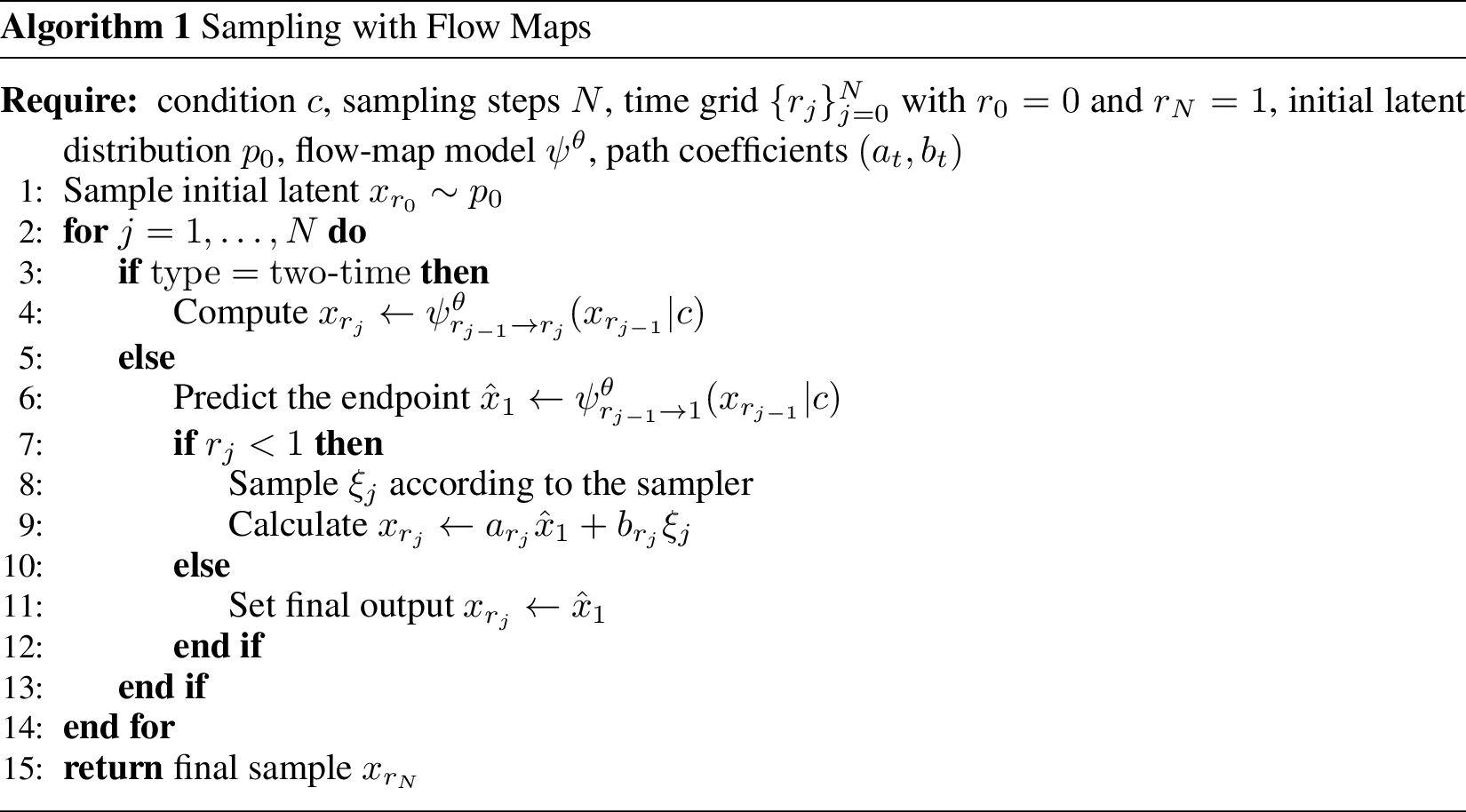
7.2.0.1 One-time endpoint maps.
One-time flow-map models, such as sCM, learn only the endpoint map \(\psi^\theta_{t\to 1}(x_t)\), which maps a state at time \(t\) directly to the data endpoint. During training, the model is therefore supervised through endpoint consistency or through the derivative-based transport constraint obtained by setting \(r=1\) in 12 . In other words, the model is not trained to represent arbitrary transitions \(\psi_{t\to r}\) for \(r<1\). At sampling time, this means that an intermediate transition from \(t\) to \(r\) cannot be obtained by directly querying a learned map \(\psi^\theta_{t\to r}\). Instead, the model first predicts the endpoint \(\hat{x}_1 = \psi^\theta_{t\to 1}(x_t)\), and then constructs an intermediate state using the prescribed probability path. For an affine path, this has the form \(x_r = a_r \hat{x}_1 + b_r \xi\), \(\xi\sim\mathcal{N}(0,I)\), or its deterministic counterpart under a fixed sampling rule. Thus, one-time models perform few-step generation by repeatedly predicting the endpoint and projecting back to intermediate noise levels according to the path schedule. This makes endpoint-map models simple and efficient, but less flexible for arbitrary finite-time transitions.
7.2.0.2 Two-time flow maps.
Two-time flow-map models, such as MeanFlow, directly parameterize transitions between arbitrary time pairs, \(\psi^\theta_{t\to r}(x_t)\), \(0\leq t,r\leq 1\). For example, MeanFlow represents this transition through the average velocity \(\psi^\theta_{t\to r}(x_t)= x_t+ (r-t)u^\theta_{t\to r}(x_t)\). During training, the model is supervised over sampled time pairs \((t,r)\) using the derivative identity derived from the flow-map transport equation. At sampling time, a finite-time transition is obtained directly by evaluating the learned two-time map: \(x_r=\psi^\theta_{t\to r}(x_t)\). Therefore, two-time models naturally support arbitrary sampling grids and can take long-range jumps between any selected time points.
7.2.0.3 Implications for Flow-Map GRPO.
This distinction determines how ASFMC is instantiated during RL post-training. For two-time flow maps, the model already provides access to \(\psi^\theta_{t\to r}\) for arbitrary time pairs, so both local anchors and endpoint anchors can be used to stochasticize a finite-time transition. In contrast, for one-time endpoint maps, the model only provides \(\psi^\theta_{t\to 1}\) and does not directly provide short local transitions such as \(\psi^\theta_{r\to r+\Delta r}\). Therefore, the local-anchor construction is not directly available for one-time models, and we use the endpoint anchor to define the stochastic policy transition.
8 Missing Proofs↩︎
8.1 Proof of 2↩︎
8.1.0.1 Theorem 2
(Long-range SDE transitions require stochastic integration) Let \(X_s\) solve the path-preserving SDE 4 and let \(\psi_{t\to r}\) be the deterministic flow map induced by the ODE 1 . For a non-infinitesimal interval \(t<r\), the exact SDE transition is generally not representable as a simple additive Gaussian perturbation of a deterministic function of the flow maps: \[X_r=G_{t,r}(X_t;\psi, d\psi,...)+ A_{t,r}\epsilon,\qquad \epsilon\sim\mathcal{N}(0,I),\] where \(A_{t,r}\) is independent of the input sample and \(G_{t,r}(X_t;\psi,d\psi,\ldots)\) denotes a deterministic functional of the flow-map family \(\psi\) and its derivatives. Instead, the exact transition must be expressed by the stochastic integral \(X_r=X_t+\int_t^r b_s(X_s)ds+\int_t^r \sigma_s dW_s\), where \(b_s(x) = u_s(x) + \frac{\sigma_s^2}{2}\nabla_x\log p_s(x)\), except for special linear-Gaussian dynamics.
Proof. It suffices to show that the exact SDE transition is generally non-Gaussian on an arbitrarily small but finite interval. Indeed, if a representation of the form \(X_r= G_{t,r}(X_t;\psi,d\psi,\ldots) + A_{t,r}\epsilon\), \(\epsilon\sim\mathcal{N}(0,I)\), were valid for general finite-time transitions, then, conditioned on \(X_t=x\), the law of \(X_r\) would be Gaussian. In particular, its third centered moment would have to vanish. We show that this is not true for a generic nonlinear SDE, even for the special case \(r=t+h\) with \(h>0\).
We prove the obstruction in one dimension; the multidimensional case follows either by considering one-dimensional systems or by applying the same argument to scalar projections. Consider the scalar SDE \[dX_s=b_s(X_s)\,ds+\sigma_s\,dW_s,\] where \(b_s\) is smooth and \(\sigma_s>0\) is state-independent. Fix \(X_t=x\) and set \(r=t+h\). The exact solution satisfies \[X_{t+h} = x + \int_t^{t+h} b_s(X_s)\,ds + \int_t^{t+h}\sigma_s\,dW_s .\] Thus, the transition depends on the full stochastic trajectory \(\{X_s\}_{s\in[t,t+h]}\).
Let \[\mu_h = \mathbb{E}[X_{t+h}\mid X_t=x], \qquad \kappa_3(h) = \mathbb{E} \left[ (X_{t+h}-\mu_h)^3 \mid X_t=x \right]\] be the conditional mean and third centered moment. A short-time expansion of the diffusion transition gives \[\kappa_3(h) = \sigma_t^4\,\partial_{xx}b_t(x)\,h^3 + o(h^3). \label{eq:kappa395expansion}\tag{13}\] For completeness, we outline the calculation. Freezing the coefficients at time \(t\) and using the local infinitesimal generator \[\mathcal{L}_t f(x) = b_t(x)\partial_x f(x) + \frac{\sigma_t^2}{2}\partial_{xx}f(x),\] the diffusion semigroup satisfies \[\mathbb{E}[f(X_{t+h})\mid X_t=x] = f(x) + h\mathcal{L}_t f(x) + \frac{h^2}{2}\mathcal{L}_t^2 f(x) + \frac{h^3}{6}\mathcal{L}_t^3 f(x) + o(h^3).\] Applying this expansion to \(f(x)=x\), \(f(x)=x^2\), and \(f(x)=x^3\), and substituting the resulting raw moments into \[\begin{align} \kappa_3(h) &= \mathbb{E}[X_{t+h}^3\mid X_t=x] - 3 \mathbb{E}[X_{t+h}\mid X_t=x]\, \mathbb{E}[X_{t+h}^2\mid X_t=x] \\ &\qquad + 2 \mathbb{E}[X_{t+h}\mid X_t=x]^3, \end{align}\] all terms up to order \(h^2\) cancel, and the leading term is exactly \[\kappa_3(h) = \sigma_t^4\,\partial_{xx}b_t(x)\,h^3 + o(h^3).\] The same leading term is obtained for smooth time-inhomogeneous coefficients by the corresponding Itô–Taylor expansion; the displayed generator calculation captures the local spatial-curvature obstruction. Therefore, whenever \(\partial_{xx}b_t(x)\neq 0\), the third centered moment is nonzero for all sufficiently small but finite \(h>0\). Hence the conditional transition law of \(X_{t+h}\) given \(X_t=x\) is not Gaussian. This contradicts any representation of the form \[X_{t+h} = G_{t,t+h}(x;\psi,d\psi,\ldots) + A_{t,t+h}\epsilon, \qquad \epsilon\sim\mathcal{N}(0,I),\] whose conditional distribution is Gaussian and therefore has zero third centered moment.
Since the interval \(t\to t+h\) is a finite, nonzero transition and is a special case of \(t\to r\), this already rules out such a simple additive-Gaussian representation for general finite-time SDE-induced flow-map transitions. Thus, for nonlinear drift fields, the exact SDE transition must be described through stochastic integration over the full random path. Only in the special linear-Gaussian case, where the drift is affine in the state and the diffusion is state-independent, does the finite-time SDE transition remain Gaussian. ◻
8.2 Proof of 4↩︎
8.2.0.1 Theorem 4
(error of the local-anchor approximation) Let \(\tilde{X}_r^\star\) denote the exact sample obtained by running the reverse-time SDE transition \(p_{r| \tau}(\cdot| X_\tau)\) from \(\tau=r+\Delta r\) to \(r\), where \(X_r=\psi_{t\to r}(X_t)\) and \(X_\tau=\psi_{r\to r+\Delta r}(X_r)\). Let \(\tilde{X}_r^{\mathrm{loc}}\) denote the local-anchor approximation \(\tilde{X}_r^{\mathrm{loc}} = X_r - \Delta r\lambda^2[ \frac{\dot{a}_r}{a_r}X_r-u_r(X_r)] + \sigma_r\sqrt{\Delta r}\xi\), \(\xi\sim\mathcal{N}(0,I)\), where \(\sigma_r=\lambda\sqrt{\frac{2b_r(\dot{a}_r b_r-a_r\dot{b}_r)}{a_r}}\). Assume that \(u_s(x)\), \(a_s\), \(b_s\), and \(\sigma_s\) are smooth with bounded derivatives in a neighborhood of the trajectory. Then the local-anchor approximation satisfies the strong error bound \[\|\tilde{X}_r^\star - \tilde{X}_r^{\mathrm{loc}}\|_{L^2}= O((\Delta r)^{3/2}).\]
Proof. Define the reverse-time drift \[B_s(x) = u_s(x) - \frac{\sigma_s^2}{2}\nabla_x\log p_s(x).\] The exact reverse-time SDE transition from \(\tau=r+\Delta r\) to \(r\) can be written as \[\tilde{X}_r^\star = X_\tau - \int_r^\tau B_s(X_s)ds + \int_r^\tau \sigma_sdW_s .\] By the Euler–Maruyama local expansion, using the same Gaussian increment \(\xi\sim\mathcal{N}(0,I)\), we have \[\tilde{X}_r^\star = X_\tau - \Delta rB_\tau(X_\tau) + \sigma_\tau\sqrt{\Delta r}\xi + R_{\mathrm{sde}}, \qquad \|R_{\mathrm{sde}}\|_{L^2}=O((\Delta r)^{3/2}).\] For the affine probability path, the score satisfies \[\nabla_x\log p_s(x) = \frac{a_su_s(x)-\dot{a}_s x}{b_s(\dot{a}_s b_s-a_s\dot{b}_s)}.\] Using \(\sigma_s^2=\lambda^2\frac{2b_s(\dot{a}_s b_s-a_s\dot{b}_s)}{a_s}\), the reverse-time drift becomes \[B_s(x) = u_s(x) - \lambda^2 [ u_s(x) - \frac{\dot{a}_s}{a_s}x ] = (1-\lambda^2)u_s(x) + \lambda^2\frac{\dot{a}_s}{a_s}x .\] Since \(\tau=r+\Delta r\) and the coefficients are smooth, \[B_\tau(X_\tau) = B_r(X_r) + O(\Delta r), \qquad \sigma_\tau = \sigma_r + O(\Delta r).\] Therefore, \[\tilde{X}_r^\star = X_\tau - \Delta rB_r(X_r) + \sigma_r\sqrt{\Delta r}\xi + O((\Delta r)^{3/2})\] in \(L^2\). For the short deterministic segment \(r\to\tau\), discretizing the ODE gives \[X_\tau = \psi_{r\to r+\Delta r}(X_r) = X_r+\Delta ru_r(X_r)+O((\Delta r)^2).\] Substituting this expression and the formula for \(B_r\) gives \[\begin{align} \tilde{X}_r^\star &= X_r + \Delta ru_r(X_r) - \Delta r [ (1-\lambda^2)u_r(X_r) + \lambda^2\frac{\dot{a}_r}{a_r}X_r ] + \sigma_r\sqrt{\Delta r}\xi + O((\Delta r)^{3/2}) \\ &= X_r - \Delta r\lambda^2 [ \frac{\dot{a}_r}{a_r}X_r-u_r(X_r) ] + \sigma_r\sqrt{\Delta r}\xi + O((\Delta r)^{3/2}). \end{align}\] The leading terms are exactly \(\tilde{X}_r^{\mathrm{loc}}\). Hence \[\| \tilde{X}_r^\star - \tilde{X}_r^{\mathrm{loc}} \|_{L^2} = O((\Delta r)^{3/2}),\] which proves the claim. ◻
9 Experiment Details↩︎
9.1 Text-to-Image Post-Training Details↩︎
9.1.0.1 Base checkpoints.
We use the FLUX.1-lite few-step generators released by T2I-Distill [21]. The released checkpoints include both MeanFlow and sCM variants. MeanFlow is treated as a two-time flow-map model, which directly parameterizes transitions \(\psi^\theta_{t\to r}\), while sCM is treated as a one-time endpoint flow-map model, which predicts \(\psi^\theta_{t\to 1}\). For each method, the “Base” model denotes the corresponding released T2I-Distill checkpoint without any RL post-training. The post-trained model denotes the same frozen base generator plus a reward-specific LoRA adapter trained with Flow-Map GRPO.
9.1.0.2 Reward-specific post-training.
We train separate LoRA adapters for three reward families: \[R \in \{\mathrm{PickScore},\;\mathrm{OCR},\;\mathrm{GenEval}\}.\] For each reward, the model is post-trained on the corresponding prompt set and the reward is evaluated on the final generated image [10]. All reward-specific runs share the same training protocol unless otherwise stated. In particular, the pretrained generator is frozen and only the LoRA adapter is updated. This setup allows us to evaluate whether Flow-Map GRPO can improve few-step flow-map generators without full-parameter finetuning.
9.1.0.3 Flow-Map GRPO rollout.
During RL post-training, we use \(K=4\) stochastic flow-map transitions for all models and all rewards. In implementation, the sampler uses a five-node rollout schedule, where four transitions are valid stochastic policy steps and the final endpoint transition is deterministic. The stochastic transitions are used to compute policy likelihood ratios, while the final deterministic transition is used only to obtain the decoded image for reward evaluation. For a prompt \(c\), we sample a group of \(G\) trajectories, compute the final-image rewards, normalize the rewards into group-level advantages, and optimize the LoRA policy with the clipped GRPO objective in 9 .
9.1.0.4 Common training hyperparameters.
Unless otherwise specified, the following hyperparameters are shared across PickScore, OCR, and GenEval post-training runs, and across the MeanFlow and sCM backbones.
| Hyperparameter | Value |
|---|---|
| Base model | T2I-Distill FLUX.1-lite MeanFlow / sCM checkpoints |
| Trainable parameters | LoRA only |
| Frozen parameters | Pretrained flow-map generator |
| Resolution | \(512 \times 512\) |
| Guidance scale | \(3.5\) |
| Max text sequence length | \(256\) |
| Stochastic policy steps | \(K=4\) |
| Images per prompt / group size | \(G=24\) |
| Training batch size | \(3\) per GPU |
| Number of GPUs | \(8\) A100 GPUs |
| Mixed precision | bf16 |
| Gradient accumulation steps | \(24\) |
| Optimizer | AdamW |
| Learning rate | \(3\times 10^{-4}\) |
| Adam betas | \((0.9, 0.999)\) |
| Weight decay | \(10^{-4}\) |
| Max gradient norm | \(1.0\) |
| GRPO clip range | \(10^{-4}\) |
| Advantage clipping | \(5\) |
| KL coefficient \(\beta\) | \(0.0\) |
| EMA | enabled |
| EMA decay | \(0.9\) |
| EMA update interval | \(8\) optimizer steps |
| Seed | \(42\) |
9.1.0.5 LoRA configuration.
All post-training runs use the same LoRA architecture. The LoRA rank is set to \(64\), the LoRA scaling factor is set to \(128\), and the LoRA dropout is set to \(0.0\). We apply LoRA to the attention projections and feed-forward projections of the FLUX transformer: \(\texttt{attn.to\_q}\), \(\texttt{attn.to\_k}\), \(\texttt{attn.to\_v}\), \(\texttt{attn.to\_out.0}\), \(\texttt{attn.add\_q\_proj}\), \(\texttt{attn.add\_k\_proj}\), \(\texttt{attn.add\_v\_proj},\) \(\texttt{attn.to\_add\_out}\), \(\texttt{ff.net.0.proj}\), \(\texttt{ff.net.2}\), \(\texttt{ff\_context.net.0.proj}\), \(\texttt{ff\_context.net.2}\) following [10]
9.1.0.6 Advantage normalization and GRPO objective.
For each prompt group, rewards are gathered across devices and normalized before the policy update. We use per-prompt reward statistics together with a global batch standard deviation. Concretely, for a trajectory \(i\) associated with prompt \(c\), the advantage is computed as \[\hat{A}^i = \frac{ R(x^i_1|c)-\mu_c }{ \sigma_{\mathrm{global}}+\epsilon_{\mathrm{std}} },\] where \(\mu_c\) is the running per-prompt reward mean, \(\sigma_{\mathrm{global}}\) is the reward standard deviation computed over the gathered rollout batch, and \(\epsilon_{\mathrm{std}}=10^{-4}\) is a numerical stabilizer. The policy update recomputes the log probability of each stochastic ASFMC transition and applies the clipped GRPO objective.
9.1.0.7 Stochasticization during training.
For MeanFlow, which directly parameterizes two-time flow maps, we instantiate ASFMC on each stochastic segment. The rollout uses a post-flow stochastic kernel with stochasticity enabled during training. The flow-map delta is set to \(0.03\), the terminal base sigma is set to \(0.05\), and the post-SDE and endpoint noise levels are set to \(0.7\) during training. The final endpoint segment is deterministic. For sCM, which predicts endpoint maps, we use the endpoint-anchor version of ASFMC described in 3.2.2. In both cases, only the stochastic ASFMC transitions contribute to the GRPO likelihood-ratio objective.
9.1.0.8 Evaluation protocol.
All reported evaluations are deterministic. We disable the training-time stochasticity by setting the evaluation post-SDE and endpoint noise levels to zero. The base checkpoint and the corresponding LoRA checkpoint are evaluated with identical resolution, guidance scale, random seed, and inference schedule within each model family. We report task-level, perceptual, and preference-based metrics, including GenEval, OCR accuracy, PickScore, aesthetic score, DQA, ImageReward, and UniReward.
10 Additional Results↩︎
10.1 MeanFlow - OCR↩︎


10.2 MeanFlow - PickScore↩︎


10.3 Consistency Model - OCR↩︎


10.4 Consistency Model - PickScore↩︎


