Scalable Security and Migration-Aware SFC Provisioning in LEO Satellite Networks
July 01, 2026
Abstract
leo satellite constellations are emerging as a backbone for global 6G connectivity, where independent tenant slices share orbital infrastructure, each requiring an ordered chain of security vnfs. Because onboard computation and networking are scarce, slices cannot be given dedicated vnfs. They must share instances on the same satellites, enlarging the attack surface and exposing tenants to cross-slice side-channel risk. This exposure shifts continually as visibility, orbital motion, and the inter-satellite topology change in time (epochs), making vnf migration a structural necessity that couples resource efficiency, service continuity, and security isolation into a single problem. We formulate this security- and migration-aware sfc placement as a multi-slice milp whose core is a co-location risk model, grounded in ISO/NIST principles and supported by analytic bounds, in which we separate avoidable migrations from those forced by orbital motion. Because the joint program scales quadratically with the cross-slice co-location terms, we develop an admm-inspired penalized per-slice best-response decomposition that recasts the coupling as a linear per-slice penalty, yielding independent subproblems through sequential (S-admm) and parallel, collision-repaired (P-admm) schedules. Simulations over a Walker-Delta satellite constellation show that the proposed framework eliminates co-location risk, reduces sfc migrations, and sustains full delay compliance, while remaining feasible within the per-epoch budget for slice counts where the monolithic security-aware milp is intractable.
application programming interface common api framework deep packet inspection
leo satellites, sfc placement, admm decomposition, security-aware optimization, vnf migration, 6G.
1 Introduction↩︎
Low Earth orbit leo satellite megaconstellations emerge as critical infrastructure for global 6G connectivity [1]. leo megaconstellations such as SpaceX Starlink, Amazon Kuiper, and OneWeb place thousands of satellites at altitudes of 340-1200 km, delivering broadband coverage with low latency [2]. The integration of leo backhaul and access capacity into 5G and next-generation 6G radio access networks (RANs) has motivated a growing interest in on-orbit edge computing, offloading latency-sensitive and security-demanding processing from terrestrial data centres to satellite computing nodes [3].
In multi-slice deployments where independent organizations share the same orbital infrastructure, security processing for each slice is naturally realized as an ordered chain of software-defined virtual network functions (vnfs) [4], forming a sfc that may include fw, ids, tm, siem, and encryption functions [5]. The orchestration problem of deciding which satellite hosts which vnf instance for which slice’s user is the main sfc placement problem studied in this paper.
This placement problem is significantly more challenging in orbital networks than in terrestrial environments due to the highly dynamic nature of leo constellations. On one hand, unlike ground networks where topology changes are relatively infrequent, the connectivity graph in leo systems evolves continuously as satellites move along their orbital trajectories [6]. For example, satellites operating at an altitude of approximately \(550\) km complete an orbit around the Earth in roughly \(90\) minutes and remain visible to a given ground user for only \(5\)–\(10\) minutes. Consequently, at each orchestration epoch, the network topology may differ substantially. Specifically, isl links are reconfigured, end-to-end propagation delays and shortest-path routes vary, and the set of satellites capable of serving a particular user changes continuously [7]. This persistent topology evolution tightly couples sfc placement decisions with the temporal dynamics of the constellation, making service-chain orchestration more complex than in static or slowly varying terrestrial networks. Consequently, epoch-by-epoch (i.e., per time window) adaptive re-optimization is mandatory [8]. Such re-optimization is not free, as it leads to relocating a running vnfs, transferring its run-time state (e.g., ids’s or siem’s detection state, and encryption session keys) across the ISL mesh, and interrupting the traffic flow and momentarily degrading the security service the SFC chain is meant to provide [9]. A rotating topology forces a baseline of relocations that no objective can prevent. Hence, each re-optimization must penalize only avoidable migrations, in which the prior satellite remains visible and capacity-feasible. Yet, the solver relocates the vnfs to improve the single-epoch objective. Forced migrations, where the prior satellite has dropped below the elevation threshold or has become capacity-infeasible, are tolerated. A myopic solver that treats all migrations uniformly over-penalizes necessary handoffs and under-penalizes controllable churn [5].
On the other hand, when functions of different slices share the same vnf instance in a satellite, confidential traffic and cryptographic material may be exposed to cross-slice side-channel attacks such as cache-timing [10] and co-resident memory probing [11]. Because the topology changes every epoch, this exposure shifts dynamically and must be mitigated by a security objective embedded within the placement optimization strategy.
Since VNF migration cost and co-location risk trade against each other, and co-location couples otherwise independent slices, the placement is chosen by a single joint optimization that minimizes both avoidable-migration cost and security risk over all slices. The main scalability challenge is due to the fact that the joint all-slice formulation introduces large binary co-location indicator variables, one for each ordered pair of (slice, sfc’s vnf) tuples sharing the same vnf instance in a particular satellite. This quadratic growth in slice counts renders the joint solution computationally intractable at a practical scale, motivating a principled decomposition strategy.
Based on the above, four requirements should be taken into account: (i) adaptation to dynamic leo topology through epoch-by-epoch re-optimization, (ii) distinction between avoidable and forced migrations, (iii) quantifiable cross-slice co-location risk objective, and (iv) tractable decomposition as the slice count grows. Prior work partially addressed these requirements, falling into four threads. First, terrestrial milp/heuristic sfc placement [12]–[15] established algorithmic baselines, but assumed static substrates without leo topology dynamics or multi-tenant security objectives. Second, vnf and sfc orchestration for leo satellite networks [16]–[19], spanning ilp decompositions [20], [21], demand-triggered migration heuristics [9], graph-attention and cooperative learning methods [22], [23], and flexible resource allocation [24], handled epoch-driven topology change but did not formalize cross-slice co-location security risk as a quantifiable multi-slice objective, even when serving multiple slices, such as [24], [25], thus overlooking inter-slice security coupling and the avoidable/forced migration distinction. Third, sfc orchestration in sagin [26]–[31] extended this concept to heterogeneous multi-segment architectures, but likewise lacked security-aware multi-slice objectives and the avoidable/forced distinction. Fourth, security-aware VNF and sfc embedding [32]–[36] enforced isolation and protection through physical separation, dedicated backup paths, or threat-aware scheduling, but only in terrestrial contexts without leo-specific dynamic co-location risk modelling.
To the best of our knowledge, no prior work fully satisfied the four requirements. To address this gap, we present here a novel security- and migration-aware sfc placement framework for leo satellite networks. The proposed framework formulates a joint multi-slice milp with McCormick-linearized co-location risk and an avoidable-migration epigraph, then applies an admm-inspired penalized per-slice best-response decomposition [37], [38] that transfers the cross-slice co-location coupling to a linear per-slice penalty. Two coordinated schedules are proposed and analyzed, namely a sequential Gauss-Seidel variant (S-admm) that refreshes a cross-slice occupancy estimate within each sweep, and a parallel variant (P-admm) that solves all slices concurrently and restores coordination through a deterministic collision-repair pass.
The main contributions of the paper are as follows:
Security- and Migration-Aware Formulation: We formulate security- and migration-aware sfc placement in leo constellations as a single-epoch multi-slice milp, subject to per-satellite CPU capacity, isl capacity, and per-user e2e delay constraints.
Scalable Decomposition: To overcome the quadratic growth of co-location variables that renders the joint milp intractable, we develop an admm-inspired penalized per-slice best-response decomposition that reduces the problem to separable per-slice subproblems. Since a naive separable penalty leaves the cross-slice coupling inactive, we further develop two coordination schedules that restore it: a sequential Gauss-Seidel occupancy refresh (S-admm) and a parallel Jacobi schedule with deterministic collision repair (P-admm).
Validation: We evaluate the framework on a satellite Walker-Delta constellation across a range of slice counts. The proposed methods reduce co-location risk by orders of magnitude relative to security-unaware optimization, remain feasible within the per-epoch budget at slice counts, for which the monolithic security-aware milp times out, and expose a controllable security-migration trade-off between the two decomposition schedules.
The remainder of the paper is organized as follows. Section 2 provides an overview of the related work. Section 3 presents the system model and Section 4 formulates the security- and migration-aware placement problem. Section 5 develops the proposed S-admm and P-admm decompositions. Section 6 describes the simulation setup and Section 7 presents the experimental results. Finally, Section 8 concludes the paper.
2 Related Work↩︎
2.6pt
Integrating sdn and nfv into leo satellite networks raises a scheduling problem. Indeed, limited on-board resources must be allocated across a topology that restructures at every orbital epoch. Early studies cast the problem as an integer program over a time-evolving graph. For example, Jia et al. formulated vnf orchestration in software-defined leo small-satellite networks as an ilp targeting resource minimization and solved it through a Dantzig-Wolfe decomposition with column generation [20], [21]. In contrast, Yan et al. reused vnf instances across concurrent flows to lower initialization delay and raise profit [42]. Building toward more heterogeneous service models, Ahsan et al. generalized these single-service formulations to a multi-slice eMBB/mMTC milp solved by successive convex approximation (SCA) with epoch-aware path reconfiguration [24].
Heuristic, temporal, and look-ahead studies instead track the structure imposed by orbital motion at a lower cost. For example, Petrosino et al. allocated sfcs among leo CubeSats over a planning horizon under intermittent visibility [27]. Moreover, Geng et al. deferred relocation until arriving requests can no longer be accommodated [9]. This demand-triggered migration heuristic is proven to approach the offline optimal cost. Liu et al. jointly reduced sfc migration frequency, delay, and jitter in SAGIN. Exploiting orbital regularity, Gao et al. used trajectory predictions [39] and later a potential-game formulation with a decentralized Nash-equilibrium solver [40] for location-aware placement, while Xia et al. introduced the chaining-orbit concept for delay-aware service chaining under uncertain isl delays [41]. Closest to the present work is our previous study [5], where we reduced handovers and security-function migrations through temporal stability regularization, warm-start seeding, and hierarchical decomposition of user association and sfc placement.
Recently, learning-based studies have addressed the scale and non-stationarity of large constellations. For instance, He et al. cast sfc orchestration in dynamic leo networks as an integer nonlinear program (INLP) and solved it with a graph attention network (GAT) that jointly maximizes service acceptance and load fairness [22]. Similarly, Doan et al. addressed joint vnf caching and placement through cooperative multi-agent Q-learning augmented by Bayesian optimization [23]. Alternatively, Jia et al. combined an ilp formulation with a double deep Q-network (DDQN) over a reconfigurable time-expansion graph to resolve inter-task resource conflicts and urgency constraints in SAGIN [45]. Other works focused on the energy efficiency of the placement strategy. For example, Chen et al. proposed a battery-aware proximal-policy-optimization (PPO) framework for sfc placement under fluctuating satellite energy levels [43], while Liu et al. developed multi-objective heuristics for satellite optical networks that jointly balance battery lifetime, e2e latency, and resource utilization under eclipse-driven power cycling [44].
The aforementioned studies have progressively broadened the sfc and vnf placement objective from resource efficiency toward service acceptance, latency, energy, and migration cost, and have evolved from exact solvers through heuristics to learning-based policies. Across all the above works, none formalized cross-slice co-location security risk as a quantifiable, optimizable objective grounded in established security standards.
Security-aware vnf placement has grown in terrestrial sfc contexts along two threads. The first enforces physical isolation as a combinatorial constraint. For instance, Gao et al. proposed multi-tenant isolation as weighted hypergraph matching that forbids co-locating conflicting tenants [34], while Wang et al. reoriented this toward survivability with asymmetric dedicated protection across primary/backup chains [35]. The second relaxes hard isolation into learned security-level requirements. For example, Zhang et al. encoded node-level security demands into the substrate features of an rl policy [46], and Dubba et al. added an explicit adversary model with sla-enforcing heuristics trading cost against security [36]. However, these works operated in terrestrial or technology-agnostic settings and treated security as a static, per-node attribute. None of these works model co-location risk as a function of data sensitivity, slice criticality, and bilateral isolation policy grounded in ISO/NIST risk management principles, namely the ISO 31000 likelihood\(\,\times\,\)consequence risk structure [47] and the NIST SP 800-53 boundary- and process-isolation control families [48]. This distinction is decisive in the LEO setting, where co-location exposure is not a one-time design constraint but an epoch-by-epoch objective that shifts as the constellation rotates, and thus should be embedded within the adaptive placement optimization approach.
This work closes the above gaps by proposing the first multi-slice security-aware milp for leo sfc placement, combining a formally grounded risk model with analytic bounds and an admm decomposition that keeps the optimization tractable. Table 1 positions reviewed works against the contributions of the proposed framework.
3 System Model↩︎
3.1 Network Model↩︎
We consider a Walker-Delta leo satellite network comprising \(S\) satellites distributed across \(P\) orbital planes, with \(S/P\) satellites per plane, orbital altitude \(h_{\text{orb}}\) km, and inclination \(\iota\) degrees. Let \(\mathcal{S}= \{1,\ldots,S\}\) denote the satellite index set. Time is discretised into orchestration epochs indexed by \(t \in \mathcal{T}= \{0,1,\ldots,T-1\}\), each of duration \(\Delta t\) seconds [49]. At each epoch \(t\), the network state is captured by a topology snapshot \(\mathcal{G}^{(t)} = \bigl(\mathcal{S},\;\mathcal{E}^{(t)},\;\boldsymbol{d}^{(t)},\;\boldsymbol{c}^{(t)},\; \boldsymbol{p}^{(t)}\bigr),\) where \(\mathcal{E}^{(t)} \subseteq \mathcal{S}\times \mathcal{S}\) is the directed isl graph, \(\boldsymbol{d}^{(t)}\) are the corresponding propagation delays, \(\boldsymbol{c}^{(t)}\) are per-satellite CPU capacities, and \(\boldsymbol{p}^{(t)} = \{\boldsymbol{r}_s^{(t)}\}_{s \in \mathcal{S}}\) are the satellite position vectors in \(\mathbb{R}^3\). The isl graph \(\mathcal{E}^{(t)}\), the propagation delays \(\boldsymbol{d}^{(t)}\), and user-satellite visibility are all derived from \(\boldsymbol{p}^{(t)}\), which is recomputed in each epoch as the constellation evolves [6]. Table 2 summarizes the complete notation used in this paper.
| Symbol | Definition |
|---|---|
| \(\calS\), \(S\) | Satellite set and cardinality |
| \(\calN\), \(N\) | Slice set and cardinality |
| \(\calF\) | VNF type set |
| \(\calI\), \(I\) | Instance index set and cardinality |
| \(\calU_n\), \(U_n\) | User set and size for slice \(n\) |
| \(L_n\) | Chain length of slice \(n\) |
| \(f_l^n\) | VNF type at position \(l\) of chain \(n\) |
| \(R_f\) | Security sensitivity of function \(f\) |
| \(C_n\) | Criticality of slice \(n\) |
| \(\Phi_{n,n'}\) | Isolation policy coefficient |
| \(w_{n,n'}^{f}\) | Risk weight (Definition [def:risk95weight]) |
| \(D_f^{\text{mig}}\) | Migration disruption cost for function \(f\) |
| \(O_{f,i,s}^{\text{actv}}\) | Activation CPU overhead of instance \((f,i,s)\) |
| \(O_{f,i,s}^{\text{incr}}\) | Per-user CPU cost of instance \((f,i,s)\) |
| \(O_{f,i,s}^{\text{proc}}\) | Processing delay of instance \((f,i,s)\) (ms) |
| \(\mathcal{C}_s^{\text{cpu}}\) | CPU capacity of satellite \(s\) |
| \(\bar{T}_{n,u}\) | E2E delay budget for user \(u\) in slice \(n\) (ms) |
| \(d_{s,s'}^{\text{SP}}\) | Shortest-path ISL delay \(s \to s'\) (ms) |
| \(d_{n,u,s}^{\text{acc}}\) | Access delay: user \(u\) of slice \(n\) to satellite \(s\) (ms) |
| \(\Omega_{n,u}^{(t)}\) | Visible satellite set for user \(u\) at epoch \(t\) |
| \(\pi_{n,u}^{l}\) | Prior-assignment feasibility |
| \(F_{\max}\) | Maximum concurrent flows per ISL link |
| \(\rho\) | Proximal penalty weight |
| \(\alpha_{n,f,i,s}\) | Cross-slice occupancy estimate |
| \(\delta_{\mathrm{obj}}\) | Objective-stagnation tolerance |
| \(\beta_{n,u,l}^{i,s}\) | Placement decision variable |
| \(\gamma_{f,i,s}\) | VNF activation indicator |
| \(z_{n,l}^{i,s}\) | Slice-activation indicator |
| \(y_{n,n',l,l'}^{i,s}\) | Co-location linearisation variable |
| \(\mu_{n,u}^{l}\) | Avoidable migration indicator |
| \(v_{n,u,l}^{s,s'}\) | ISL-hop McCormick variable |
| \(\sigma_{n,u}^{l}\) | stay indicator at prior assignment \((\hat\imath,\hat{s})\) |
| \(\xi_{n,u,l}^{s}\) | aggregate satellite-assignment at position \(l\) (\(\sum_i \beta_{n,u,l}^{i,s}\)) |
| \(\bar{U}\) | maximum users per slice |
| \(L_{\max}\) | maximum chain length |
At epoch \(t\), satellite \(s\) maintains isls to at most \(k\) nearest neighbours (typically \(k=4\): intra-plane fore/aft and inter-plane left/right [8]). The direct-link propagation delay between adjacent satellites \(s, s' \in \mathcal{S}\) is \(d_{s,s'}^{(t)} = \|\boldsymbol{r}_s^{(t)} - \boldsymbol{r}_{s'}^{(t)}\|_2 / c\), where \(c\) is the speed of light [6]. For non-adjacent satellite pairs \((s,s')\notin\mathcal{E}^{(t)}\), the satellite pairs’ shortest-path (SP) delay \(d_{s,s'}^{\text{SP},(t)}\) is computed via Dijkstra’s algorithm over \(\mathcal{G}^{(t)}\), at every time epoch to reflect the evolving isl graph.
Let \(\mathcal{N}= \{1,\ldots,N\}\) be the set of network slices, each representing an independent slice with a dedicated security service requirement. The security requirements of a slice \(n \in \mathcal{N}\) is characterised by an ordered sfc \(\mathcal{F}_n = \{f_1^n, f_2^n, \ldots, f_{L_n}^n\},\) where \(\mathcal{F}\) is the set of admissible security vnf types (e.g., \(\mathcal{F}= \{\text{FW}, \text{IDS}, \text{ENC}, \text{TM}, \text{SIEM}\}\)), and \(L_n = |\mathcal{F}_n|\) is the chain length. A slice \(n\) serves a set \(\mathcal{U}_n = \{1,\ldots,U_n\}\) of ground users, each with a known location (i.e., latitude and longitude). User \(u\) of slice \(n\) can communicate with satellite \(s\) at epoch \(t\) if and only if (iff) the elevation angle \(\theta_{n,u,s}^{(t)}\) satisfies \(\theta_{n,u,s}^{(t)} \geq \theta_{\min}\), where \(\theta_{\min}\) is the minimum visibility elevation angle. The visible satellite set for user \(u \in \mathcal{U}_n\) at epoch \(t\) is defined as \(\Omega_{n,u}^{(t)} = \bigl\{ s \in \mathcal{S}| \theta_{n,u,s}^{(t)} \geq \theta_{\min} \bigr\}.\) Traffic from user \(u\) must traverse the slice’s sfc in strict order \(f_1^n \to f_2^n \to \cdots \to f_{L_n}^n\), with respect to its e2e latency budget \(\bar{T}_{n,u}\) ms. For each function type \(f \in \mathcal{F}\) and satellite \(s \in \mathcal{S}\), there are \(I\) candidate vnf instances indexed by \(\mathcal{I}= \{1,\ldots,I\}\). An instance \((f, i, s)\) (with \(i \in \mathcal{I}\)) is characterised by different overheads, including fixed activation CPU overhead \(O_{f,i,s}^{\text{actv}}\), per-user incremental CPU load \(O_{f,i,s}^{\text{incr}}\), and vnf processing delay \(O_{f,i,s}^{\text{proc}}\).
3.2 Co-location Security Risk Model↩︎
The main security concern in multi-slice computing is vnf co-location. When functions of different slices share the same physical instance on the same satellite, confidential traffic flows and cryptographic material may be exposed to cross-slice side-channel attacks [11], [50], [51]. We represent this risk via a multiplicative security model inspired by ISO 31000 [47] and NIST SP 800-53 [48]. The ISO 31000 risk management vocabulary (likelihood \(\times\) consequence, risk appetite, controls) informs the multiplicative structure of Definition 1 below.
Definition 1 (Security Co-location Risk Weight). The security co-location risk weight between slices \(n, n' \in \mathcal{N}\), \(n < n'\), for function type \(f \in \mathcal{F}\) is defined as \[w_{n,n'}^{f} = R_f \cdot \Phi_{n,n'} \cdot C_n \cdot C_{n'} \;\geq 0, \label{eq:risk95weight}\qquad{(1)}\] where \(R_f\) is the security sensitivity of function type \(f\) (higher for cryptographic or intrusion-detection functions), \(C_n\) is the criticality of slice \(n\) (reflecting data classification level), and \(\Phi_{n,n'}\) is the bilateral isolation policy coefficient between slices \(n\) and \(n'\), with \(\Phi_{n,n'} = \Phi_{n',n}\) (symmetric). The multiplicative structure implies that any zero factor (zero sensitivity, zero criticality, or enforced isolation) collapses the full risk contribution to zero, consistent with zero-trust policy semantics.
The NIST SP 800-53 control families [48], relevant to multi-slice sfc isolation, include: SC-2 (Application Partitioning), SC-7 (Boundary Protection), and SC-39 (Process Isolation). These controls map to the isolation policy coefficient \(\Phi_{n,n'}\) and the activation of zero-trust enforcement (\(\Phi_{n,n'} = 0\) corresponds to full SC-39 isolation between slices \(n\) and \(n'\)). Moreover, cross-slice isolation requirement on shared infrastructure is recognized across the 5G/NFV slicing-security literature [33], [50]. Since every factor in ?? is symmetric in its slice indices, we extend the risk weight to all ordered pairs by setting \(w_{n',n}^{f} \triangleq w_{n,n'}^{f}\) for \(n' < n\).
Definition 2 (Co-location Security Risk). The co-location security risk is calculated as \[\begin{align} \mathcal{R}&= \sum_{\substack{n,n' \in \mathcal{N}\\ n < n'}} \sum_{f \in \mathcal{F}_n \cap \mathcal{F}_{n'}} \sum_{i \in \mathcal{I}} \sum_{s \in \mathcal{S}} w_{n,n'}^{f} ~ \bigl|\mathcal{A}_{n,f}^{i,s}\bigr| \cdot \bigl|\mathcal{A}_{n',f}^{i,s}\bigr|, \label{eq:risk95exact} \end{align}\qquad{(2)}\] where \(\mathcal{A}_{n,f}^{i,s}\) is the set of users of slice \(n\) assigned to instance \((f,i,s)\).
We treat each pair of co-resident cross-slice flows on a shared instance as one independent side-channel exposure [11]. The per-instance term \(|\mathcal{A}_{n,f}^{i,s}| \cdot |\mathcal{A}_{n',f}^{i,s}|\) in ?? counts these exposure pairs, generalizing the binary co-residency model standard in the side-channel literature. Following the ISO 31000 likelihood \(\times\) consequence structure, each contribution factorises into a consequence component \((R_f\,C_n C_{n'})\) and a likelihood component \((\Phi_{n,n'}\,~|\mathcal{A}_{n,f}^{i,s}|~|\mathcal{A}_{n',f}^{i,s}|)\).
Direct minimization of \(\mathcal{R}\) is intractable as it involves products of integer sums. Hence, we introduce the coarse co-location indicator \[z_{n,l}^{i,s} \in \{0,1\},\quad z_{n,l}^{i,s} = 1 \iff \exists\, u \in \mathcal{U}_n | \beta_{n,u,l}^{i,s} = 1, \label{eq:z95def}\tag{1}\] indicating whether there is a user of slice \(n\) that is served by instance \((f,i,s)\) or not, and where \(\beta_{n,u,l}^{i,s}\!\in\!\{0,1\}\) is a binary variable equals 1 iff the \(l\)-th vnf of \(\mathcal{F}_n\) is assigned to instance \(i\) on satellite \(s\) for a user \(u\) belonging to slice \(n\). For the coarse co-location indicator \(z_{n,l}^{i,s}\), we establish the following analytic bounds.
Proposition 1 (Co-location Security Risk Bounds). For any assignment \(\boldsymbol{\beta}=[\beta_{n,u,l}^{i,s}]_{n\in\mathcal{N},\;u\in\mathcal{U}_n,\; l\in\{1,\ldots,L_n\},\;i\in\mathcal{I},\;s\in\mathcal{S}}\), define the bilinear co-location indicator \[y_{n,n',l,l'}^{i,s} = z_{n,l}^{i,s} \cdot z_{n',l'}^{i,s}, \label{eq:y95bilinear}\qquad{(3)}\] where \((n,l)\) and \((n',l')\) share the same function type (\(f_l^n = f_{l'}^{n'} = f\)). Then, \(\mathcal{R}^{\text{LB}} \;\leq\; \mathcal{R}\;\leq\; \mathcal{R}^{\text{UB}}, \label{eq:risk95bounds}\) where \[\begin{align} \mathcal{R}^{\text{LB}} &= \sum_{\substack{n,n' \in \mathcal{N},\; n < n' \\l \in [L_n],\; l' \in [L_{n'}] }} \sum_{i \in \mathcal{I},\; s \in \mathcal{S}} w_{n,n'}^{f}\, ~ y_{n,n',l,l'}^{i,s}, \label{eq:risk95lb} \\[4pt] \mathcal{R}^{\text{UB}} &= \sum_{\substack{n,n' \in \mathcal{N},\; n < n' \\l \in [L_n],\; l' \in [L_{n'}] }} \sum_{i \in \mathcal{I},\; s \in \mathcal{S}} w_{n,n'}^{f}\, ~ |\mathcal{U}_n|\cdot |\mathcal{U}_{n'}|\, ~ y_{n,n',l,l'}^{i,s}. \label{eq:risk95ub} \end{align}\] {#eq: sublabel=eq:eq:risk95lb,eq:eq:risk95ub}
Proof sketch. When \(y_{n,n',l,l'}^{i,s}=1\), at least one user in \(\mathcal{U}_n\) and at least one user in \(\mathcal{U}_{n'}\) use instance \((f,i,s)\), such that \(|\mathcal{A}_{n,f}^{i,s}| \cdot |\mathcal{A}_{n',f}^{i,s}| \geq 1 = y_{n,n',l,l'}^{i,s}\), establishing the lower bound. Since \(|\mathcal{A}_{n,f}^{i,s}| \leq |\mathcal{U}_n|\) and \(|\mathcal{A}_{n',f}^{i,s}| \leq |\mathcal{U}_{n'}|\), their product is at most \(|\mathcal{U}_n|\cdot |\mathcal{U}_{n'}|\), establishing the upper bound. When \(y_{n,n',l,l'}^{i,s}=0\), at least one of the sets is empty, so the product is zero and all bounds are tight. ◻
Note that \(\mathcal{R}^{\text{LB}}\) in ?? can be seen as the binary co-residency risk standard in the side-channel attacks. It charges \(w_{n,n'}^{f}\) once per co-resident slice pair, independent of workload. The exact risk ?? and worst-case bound ?? satisfy \(\mathcal{R}^{\text{LB}} \le \mathcal{R}\le \mathcal{R}^{\text{UB}}\) and serve as evaluation metrics. Since \(w_{n,n'}^{f}\ge 0\), \(\mathcal{R}^{\text{LB}}=0\) iff \(\mathcal{R}=0\) (Definition 2). Away from zero, the per-slice consolidation provides \(\mathcal{R}= U^{2}\,\mathcal{R}^{\text{LB}}\), thus, \(\mathcal{R}^{\text{LB}}\) is an order-preserving constant-factor surrogate for \(\mathcal{R}\).
4 Problem Formulation↩︎
This section formalizes the single-epoch placement problem, defines the binary decision variables, and states the feasibility constraints. For readability, the epoch index \(t\) is omitted from the per-epoch variables and constants throughout the paper.
4.1 Decision Variables↩︎
The decision variables in our system are as follows:
\(\beta_{n,u,l}^{i,s} \in \{0,1\}:\) vnf-usage indicator, equals 1 iff the \(l\)-th vnf of \(\mathcal{F}_n\) is assigned to instance \(i\) on satellite \(s\) for a user \(u\) belonging to slice \(n\). We refer to the triple \((n,u,l)\) as a chain placement,
\(\gamma_{f,i,s} \in \{0,1\}\): vnf activation indicator, equal to 1 iff at least one user is served by instance \((f,i,s)\),
\(z_{n,l}^{i,s}\!\in\!\{0,1\}\): instance-usage indicator, equal to 1 iff any user of slice \(n\) uses instance \((f_l^n,i,s)\),
\(\mu_{n,u}^{l}\!\in\!\{0,1\}\): avoidable-migration indicator, equal to 1 iff the prior-epoch assignment remained feasible, but the solver chose otherwise.
4.2 Constraint Set↩︎
A feasible placement must satisfy the following six constraint families, governing user-to-instance assignment (C1), instance activation (C2), satellite CPU capacity (C3), avoidable-migration accounting (C4), e2e delay (C5), and isl link capacity (C6).
(C1) Unique assignment: Each user \(u \in \mathcal{U}_n\) must be assigned to exactly one instance at each chain position \(l\) of \(\mathcal{F}_n\): \[\sum_{i \in \mathcal{I}}\sum_{s \in \mathcal{S}} \beta_{n,u,l}^{i,s} = 1, \quad \forall\, n \in \mathcal{N},\; u \in \mathcal{U}_n,\; l \in \{1,\ldots,L_n\}. \label{C1}\tag{2}\] When \(l = 1\), the summation over \(s\) is restricted to the visible satellite set \(\Omega_{n,u}^{(t)}\). The sfc’s vnfs at positions \(l>1\) may therefore reside on any satellite in \(\mathcal{S}\), including satellites not visible to the user, and are reached via the SP isl route.
(C2) Activation coupling: A vnf instance \((f,i,s)\) is activated only when used by at least one user. This vnf activation coupling is enforced by: \[\begin{align} \beta_{n,u,l}^{i,s} &\leq \gamma_{f_l^n,\,i,\,s}, \; \forall\, n \in \mathcal{N}, u \in \mathcal{U}_n, l\in \{1,\ldots,L_n\}, i \in \mathcal{I},\nonumber \\ s \in \mathcal{S}, \tag{3} \\ \gamma_{f,i,s} &\leq \sum_{\substack{n \in \mathcal{N},\; u \in \mathcal{U}_n \\ \{l|\, f_l^n = f\}}} \beta_{n,u,l}^{i,s}, \quad \forall\, f \in \mathcal{F},\; i \in \mathcal{I},\; s \in \mathcal{S}. \tag{4} \end{align}\]
(C3) Satellite CPU capacity: The total CPU load on satellite \(s\) is \[\begin{align} \text{CPU}_s &= \sum_{f \in \mathcal{F}}\sum_{i \in \mathcal{I}} O_{f,i,s}^{\text{actv}}\, ~ \gamma_{f,i,s}\nonumber \\ &+ \sum_{n \in \mathcal{N}}\sum_{u \in \mathcal{U}_n}\sum_{l=1}^{L_n}\sum_{i \in \mathcal{I}} O_{f_l^n,i,s}^{\text{incr}}\, ~ \beta_{n,u,l}^{i,s}, \label{eq:cpu95load} \end{align}\tag{5}\] Consequently, the aggregate CPU load on each satellite must not exceed its capacity: \[\begin{align} \text{CPU}_s \leq \mathcal{C}_s^{\text{cpu}}, \quad \forall\, s \in \mathcal{S}. \label{C3} \end{align}\tag{6}\]
(C4) Avoidable migration epigraph: Let denote the total migration disruption cost calculated as \[\text{Mig} = \sum_{n \in \mathcal{N}}\sum_{u \in \mathcal{U}_n}\sum_{l=1}^{L_n} D_{f_l^n}^{\text{mig}}\, ~ \mu_{n,u}^{l}, \label{eq:migcost}\tag{7}\] where \(D_{f_l^n}^{\text{mig}}\) is the migration disruption cost for the security function \(f\). Let \((\hat{\imath},\hat{s})\) denote the prior-epoch assignment of chain placement \((n,u,l)\) and \(\pi_{n,u}^{l} \in \{0,1\}\) be the precomputed feasibility flag, i.e., \(\pi_{n,u}^{l} = 1\) iff satellite \(\hat{s}\) is visible to user \(u\) at the current epoch and the residual capacity of \(\hat{s}\) can accommodate the user. We define the stay indicator as the shorthand \(\sigma_{n,u}^{l} \triangleq \beta_{n,u,l}^{\hat{\imath},\hat{s}} \in \{0,1\}\). The avoidable migration variable satisfies \(\mu_{n,u}^{l} = \max\bigl(0,\; \pi_{n,u}^{l} - \sigma_{n,u}^{l}\bigr), \label{eq:mu95prop}\) which is linearised as the three-constraint epigraph: \[\begin{align} \mu_{n,u}^{l} &\geq \pi_{n,u}^{l} - \sigma_{n,u}^{l}, \tag{8} \\ \mu_{n,u}^{l} &\leq \pi_{n,u}^{l}, \tag{9} \\ \mu_{n,u}^{l} &\leq 1 - \sigma_{n,u}^{l}. \tag{10} \end{align}\] When \(\pi_{n,u}^{l} = 0\) (prior assignment infeasible), 9 –10 force \(\mu_{n,u}^{l}=0\), excluding involuntary handovers from the penalty. The flag \(\pi_{n,u}^{l}\) is necessarily precomputed from epoch-\((t{-}1)\) information. Indeed, the current-epoch cross-slice load on \(\hat{s}\) is unknown until the joint placement is solved, so letting \(\pi\) depend on it would be circular. Hence, it estimates the residual capacity of \(\hat{s}\) from the prior committed load. The milp still enforces the exact capacity constraint 6 , such that every returned placement is feasible, while only the avoidable-versus-forced classification is approximate. If current-epoch contention forces a user off a prior satellite that appeared feasible under the \((t{-}1)\) estimate, the migration is deemed avoidable. Hence, the approximation is conservative as it can only inflate the proposed methods’ reported avoidable-migration count, but never deflate it.
(C5) e2e delay budget: The total E2E latency of each user must not exceed its budget \(\bar{T}_{n,u}\), i.e., \[\begin{gather} \underbrace{\sum_{i\in \mathcal{I},s \in \Omega_{n,u}^{(t)}} d_{n,u,s}^{\text{acc}}\, ~ \beta_{n,u,1}^{i,s}}_{\text{access delay}} + \underbrace{\sum_{l=1}^{L_n}\sum_{i \in \mathcal{I},s \in \mathcal{S}} O_{f_l^n,i,s}^{\text{proc}}\, ~ \beta_{n,u,l}^{i,s}}_{\text{processing delays}} \\ + \underbrace{\sum_{l=1}^{L_n-1}\sum_{s \in \mathcal{S}, s \neq s'} d_{s,s'}^{\text{SP}}\, ~ v_{n,u,l}^{s,s'}}_{\text{ISL propagation}} \leq \bar{T}_{n,u}, \;\forall\, n \in \mathcal{N}, u \in \mathcal{U}_n, \label{C5} \end{gather}\tag{11}\] where the McCormick variable \(v_{n,u,l}^{s,s'} \in [0,1]\) linearizes the ISL routing product (see 17 –18 below) and it is created only for reachable \((s,s')\) pairs to limit the model size.
(C6) isl link capacity: The aggregate number of user flows routed over each directed isl must not exceed the link’s flow capacity \(F_{\max}\), i.e., \[\sum_{n \in \mathcal{N}}\sum_{u \in \mathcal{U}_n}\sum_{l=1}^{L_n-1} v_{n,u,l}^{s,s'} \leq F_{\max}, \quad \forall\,(s,s') \in \mathcal{E}^{(t)}. \label{C6}\tag{12}\]
4.3 Linearisation of Bilinear Terms↩︎
The above formulations contain two classes of bilinear products that must be linearized for milp tractability. The normalization is discussed in the following two subsections.
4.3.1 Co-location Security Risk Linearisation↩︎
The indicator \(y_{n,n',l,l'}^{i,s} = z_{n,l}^{i,s} \cdot z_{n',l'}^{i,s}\) in ?? is the product of two binary variables. Since both factors are binary, the standard McCormick [52] linearisation reduces to the three-constraint LP relaxation: \[\begin{align} y_{n,n',l,l'}^{i,s} &\leq z_{n,l}^{i,s}, \tag{13} \\ y_{n,n',l,l'}^{i,s} &\leq z_{n',l'}^{i,s}, \tag{14} \\ y_{n,n',l,l'}^{i,s} &\geq z_{n,l}^{i,s} + z_{n',l'}^{i,s} - 1. \tag{15} \end{align}\] The slice-activation indicator \(z_{n,l}^{i,s}\) is related to \(\boldsymbol{\beta}\) via \[\begin{align} z_{n,l}^{i,s} \geq \beta_{n,u,l}^{i,s}, \text{ and } z_{n,l}^{i,s} \leq \sum_{u \in \mathcal{U}_n} \beta_{n,u,l}^{i,s}. \label{eq:z95ub} \end{align}\tag{16}\] Since \(\beta_{n,u,l}^{i,s}\) and \(z_{n,l}^{i,s}\) are binary and C1 guarantees \(\sum_{i\in \mathcal{I},s\in \mathcal{S}}\beta_{n,u,l}^{i,s}=1\), the relaxation of the McCormick envelope is exact. At any integer-feasible solution, \(y_{n,n',l,l'}^{i,s}\) take binary values and are exactly equal to \(z_{n,l}^{i,s} \cdot z_{n',l'}^{i,s}\).
4.3.2 ISL Delay Linearization↩︎
The isl propagation term in 11 depends on the pair of satellites hosting two consecutive vnfs. Let \(\xi_{n,u,l}^{s} \triangleq \sum_{i \in \mathcal{I}} \beta_{n,u,l}^{i,s} \in \{0,1\}\) be the aggregate satellite-assignment indicator, i.e., equal to 1 iff the \(l\)-th vnf of user \(u\) is placed on satellite \(s\), regardless of the instance. Then, the product \(\xi_{n,u,l}^{s} \cdot \xi_{n,u,l+1}^{s'}\) equals 1 when user \(u\) routes vnf \(l\) through \(s\) and vnf \((l+1)\) through \(s'\) (i.e., when the flow traverses the directed isl \((s,s')\) between hops \(l\) and \(l+1\)). This conjunction of two consecutive placement decisions is irreducibly bilinear. Therefore, we keep the aggregated indicator and introduce a single auxiliary variable \(v_{n,u,l}^{s,s'} \in [0,1]\) per reachable hop, linearized by the binary-product (McCormick) envelope as follows: \[\begin{align} v_{n,u,l}^{s,s'} \geq \xi_{n,u,l}^{s} + \xi_{n,u,l+1}^{s'} - 1, \tag{17} \\ v_{n,u,l}^{s,s'} \leq \xi_{n,u,l}^{s}, \text{ and } v_{n,u,l}^{s,s'} \leq \xi_{n,u,l+1}^{s'}, \tag{18} \end{align}\] for all chain placements \((n,u,l)\) and all satellite pairs \((s,s') \in \mathcal{S}^2\) with \(s \neq s'\) and \(d_{s,s'}^{\text{SP}} > 0\). Since C1 imposes \(\xi_{n,u,l}^{s} \in \{0,1\}\), the envelope is exact at every integer-feasible point, as 18 pins \(v_{n,u,l}^{s,s'}\) to \(0\) unless both hops are active, and 17 forces it to \(1\) when they are active. Hence, \(v_{n,u,l}^{s,s'} = \xi_{n,u,l}^{s}\,~\xi_{n,u,l+1}^{s'}\) holds.
4.4 Objective Function↩︎
The main objective is to minimize the weighted co-location security risk and vnf migration cost, as follows: \[\begin{align} \min_{\boldsymbol{\beta},\boldsymbol{\gamma},\mathbf{z},\mathbf{y},\boldsymbol{\mu}} \quad& \omega_{\text{risk}}\,\frac{\mathcal{R}^{\text{LB}}}{\bar{R}} + \omega_{\text{mig}}\, \frac{\text{Mig}}{\bar{M}} \label{eq:milp95obj}, \\[2pt] \text{s.t.} \quad & \eqref{C1}\text{--}\eqref{C6}, \eqref{eq:y95mcc1}\text{--}\eqref{eq:h95ub2}.\nonumber \end{align}\tag{19}\] The selected values of the weighting vector \((\omega_{\text{risk}}, \omega_{\text{mig}})\) reflect the importance of each term in multi-slice leo deployments. The normalization constants \(\bar{R}\) and \(\bar{M}\) are computed as analytic upper bounds in a preprocessing step, so that each normalized term lies in \([0,1]\), making the objective a convex combination that avoids scale-induced bias. The dominant variables count is from the \(y\)-variables (co-location indicators), whose number is \(O(N^2 L_{\max}^2 IS)\) in the joint formulation. This quadratic scaling motivates the admm decomposition developed in the section below.
5 Proposed admm-inspired Decomposition Framework↩︎
5.1 admm-inspired Decomposition Principle↩︎
For large constellations and several slices, the joint milp formulated in 19 is computationally intractable due to the \(O(N^2 L_{\max}^2 IS)\) co-location variables and the joint optimization over \(N ~ \sum_{n \in \mathcal{N}} U_n\) users’ combinations. We exploit the spatial separability of the problem, where the per-slice placement subproblems become independent when the activations of the other slices on each instance are fixed. Hence, we replace the joint solve with a penalized per-slice best response, i.e., an admm-inspired block decomposition [37], similar to what is used for scalable structured optimization [53]–[55]. In this work, admm is customized to multi-slice binary sfc placement with cross-slice co-location coupling. Let \(\gamma_{n,f,i,s} \in \{0,1\}\) denote the per-slice activation of instance \((f,i,s)\) by slice \(n\) (equivalently \(\max_{\{l|\,f_l^n = f\}} z_{n,l}^{i,s}\)), the slice-local counterpart of the global activation indicator \(\gamma_{f,i,s}\) in 5 . The cross-slice coupling is carried by an occupancy estimate \(\alpha_{n,f,i,s} \in [0,1]\) of the other slices’ activations on instance \((f,i,s)\), maintained across admm sweeps and initialized to \(\alpha^{(0)} = 0\).
Let \(\boldsymbol{\beta}^{(t)}\) denote the committed placement at epoch \(t\) and \(\boldsymbol{\beta}^{(t-1)}\) the previous-epoch placement used as the fixed migration reference. Also, let \(\tilde{\boldsymbol{\beta}}^{(k)}\) and \(\hat{\boldsymbol{\beta}}\) denote the merged and repaired placements, respectively, sharing the same structure. For each slice \(n\), let \(\boldsymbol{\beta}_n\), \(\boldsymbol{\gamma}_n\), and \(\boldsymbol{\mu}_n\) denote the restrictions of the placement, activation, and avoidable-migration variables to slice \(n\) (i.e., the entries \(\beta_{n,u,l}^{i,s}\), \(\gamma_{n,f,i,s}\), and \(\mu_{n,u}^{l}\) that carry slice index \(n\)). Moreover, let a superscript \(^{(k)}\) marks the value of these blocks at ADMM sweep \(k\), such that \(\boldsymbol{\beta}_n^{(k)}\) is slice \(n\)’s placement after the sweep-\(k\) solve. At each admm sweep \(k\), the x-step solves \(N\) per-slice milps as follows: \[\begin{align} \min_{\boldsymbol{\beta}_n, \boldsymbol{\gamma}_n, \boldsymbol{\mu}_n} \quad & \omega_{\text{mig}}~ \frac{\,\text{Mig}_n}{\bar{M}} + \sum_{f,i,s} \phi_{n,f,i,s}^{(k)}\,~\gamma_{n,f,i,s}, \label{eq:admm95xstep} \\ \text{s.t.} \quad & \eqref{C1},\;\eqref{C2a}\text{--}\eqref{C2b},\; \eqref{eq:c3rem},\; \eqref{C4a}\text{--}\eqref{C4c},\;\eqref{C5}, \nonumber \end{align}\tag{20}\] where the residual-capacity constraint 21 applies the joint CPU bound of constraint 6 to slice \(n\) only, against the capacity left by the other slices: \[\text{CPU}_{n,s} \;\le\; \mathcal{C}_s^{\text{cpu}} - \Lambda_{n,s}^{(k)}, \quad \forall\, s \in \mathcal{S}, }_n}\label{eq:c3rem}\tag{21}\] where \(\text{CPU}_{n,s}\) is slice \(n\)’s CPU load on satellite \(s\) and \(\Lambda_{n,s}^{(k)}\) denotes the CPU load reserved by the other slices. \(\Lambda_{n,s}^{(k)}\) is set differently by the two coordination schedules (S-admm) and (P-admm) developed in Subsections 5.2 and 5.3, respectively, which differ only in which other slices’ loads are reserved. Fig. 1 illustrates the E2E overview of the proposed framework along with the decomposition strategy.
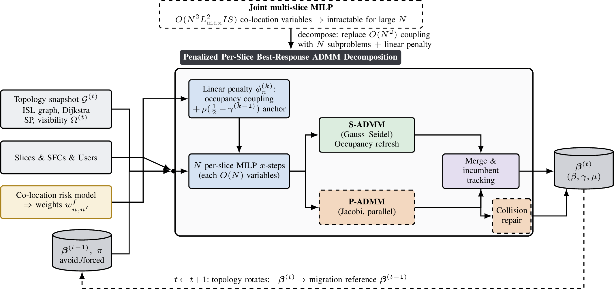
The sequential schedule (S-admm) reserves the loads of slices already solved in the current sweep (\(n' < n\)), whereas the parallel schedule (P-admm) reserves all other slices’ loads from the previous sweep (\(n' \neq n\)). Accordingly, \[\Lambda_{n,s}^{(k)} = \begin{cases} \displaystyle\sum_{n' < n} \ell_{n',s}^{(k)} & \text{(S-\gls{admm}),}\\[6pt] \displaystyle\sum_{n' \neq n} \ell_{n',s}^{(k-1)} = L_s^{(k-1)} - \ell_{n,s}^{(k-1)} & \text{(P-\gls{admm}),} \end{cases} \label{eq:residual95reserve}\tag{22}\] with \(\ell_{n,s}^{(k)} = \text{CPU}_{n,s}\) the load slice \(n\) commits on satellite \(s\) in ADMM sweep \(k\) and \(L_s^{(k)} = \sum_{n\in \mathcal{N}} \ell_{n,s}^{(k)}\). Reserving from the previous sweep is what permits P-admm’s fully parallel solves.
The co-location \(y\)-variables are absent from each per-slice subproblem and their cross-slice coupling is transferred entirely to the linear penalty \(\phi_{n,f,i,s}^{(k)}\) on the activation \(\gamma_{n,f,i,s}\), which linearizes the joint risk of the current occupancy estimates \(\{\alpha_{n',f,i,s}\}_{n' \neq n}\) as follows: \[\phi_{n,f,i,s}^{(k)} = \frac{\omega_{\text{risk}}}{\bar{R}} \sum_{\substack{n'n, \in \mathcal{N}\\n' \neq n}} w_{n,n'}^{f}\, ~ \alpha_{n',f,i,s} + \rho \Bigl(\tfrac{1}{2} - \gamma_{n,f,i,s}^{(k-1)}\Bigr), \label{eq:admm95penalty}\tag{23}\] where the first term is the linearized cross-slice co-location risk evaluated at the other slices’ occupancy, and the second is a proximal anchor of strength \(\rho > 0\) to slice \(n\)’s own activation from the preceding sweep, \(\gamma_{n,f,i,s}^{(k-1)}\) (with \(\gamma^{(0)} = 0\)), which damps inter-sweep oscillation. Instead of the dual-ascent step of consensus admm, this decomposition maintains no dual variable and the coordination is carried entirely by the primal occupancy estimate \(\alpha_{n',f,i,s}\) and the primal proximal anchor, such that \(\phi_{n,f,i,s}^{(k)}\) is a linear coefficient on \(\gamma_{n,f,i,s}\). Therefore, our approach should be viewed as a penalized best-response admm-inspired decomposition rather than a canonical consensus-admm formulation. Correspondingly, our convergence result is the best-response fixed-point guarantee of Proposition 2, rather than the primal–dual convergence guarantee associated with conventional admm. The second term in 23 is the exact linear representation of the squared proximal term \(\tfrac{\rho}{2}\lVert\gamma_{n,f,i,s}-\gamma_{n,f,i,s}^{(k-1)}\rVert^2\) under binary activation variables. Since \(\gamma \in \{0,1\}\) implies \(\gamma^2 = \gamma\), the quadratic term can be rewritten as \(\rho(\tfrac{1}{2}-\gamma_{n,f,i,s}^{(k-1)})\,~\gamma_{n,f,i,s}\) plus a constant in \(\gamma_{n,f,i,s}\). Consequently, the proximal anchor remains the previous activation state \(\gamma_{n,f,i,s}^{(k-1)}\), as in standard proximal methods, while the coefficient \(\tfrac{1}{2}\) arises solely from the binary nature of the decision variable and does not constitute an additional tuning parameter. When \(\gamma_{n,f,i,s}^{(k-1)} = 0\), the second term becomes \(+\rho/2\) interpreted as the cost of activating an instance and thus encourages retention of the previous inactive state. Conversely, when \(\gamma_{n,f,i,s}^{(k-1)} = 1\), the second term becomes \(-\rho/2\), providing an equal incentive to preserve the previous active state. These two cases are symmetric manifestations of the same proximal regularization mechanism, whose influence may be outweighed whenever the risk or migration terms yield a sufficiently large reduction in the per-slice objective.
After each x-step, the occupancy estimate is updated to match the realized activation: \[\alpha_{n,f,i,s} \leftarrow \gamma_{n,f,i,s}^{(k)}. \label{eq:admm95occ}\tag{24}\] This update is performed either immediately after each slice optimization within the sweep (S-admm, Subsection 5.2) or collectively once all slice subproblems have been solved (P-admm, Subsection 5.3). The resulting placement \(\tilde{\boldsymbol{\beta}}^{(k)}\) is then evaluated using the normalized objective \[\mathrm{obj}^{(k)} = \omega_{\text{risk}}\frac{\mathrm{Risk}^{\mathrm{LB}}}{\bar{R}}\, \bigl(\tilde{\boldsymbol{\beta}}^{(k)}\bigr) + \omega_{\text{mig}}\frac{\mathrm{Mig}}{\bar{M}}\, \bigl(\tilde{\boldsymbol{\beta}}^{(k)}\bigr), \label{eq:admm95incumbent}\tag{25}\] best-performing placement encountered thus far is retained as the incumbent solution. The iterative procedure terminates when the incumbent objective exhibits negligible improvement, \(|\mathrm{obj}^{(k)} - \mathrm{obj}^{(k-1)}| < \delta_{\mathrm{obj}}\), or when the maximum number of sweeps, \(K_{\max}\), is reached.
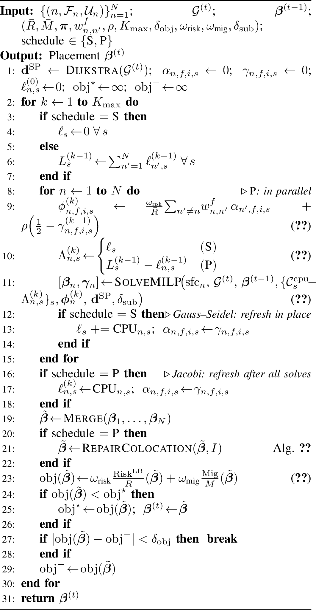
Algorithm 2 summarizes the resulting penalized best-response decomposition. The scheduling flag determines whether coordination follows the S-admm update rule of Subsection 5.2 or the P-admm update rule of Subsection 5.3.
5.2 S-admm: Sequential Gauss–Seidel Coordination↩︎
In S-admm, the \(N\) per-slice \(\mathbf{x}\)-steps are solved sequentially according to a fixed ordering, \(n = 1, 2, \ldots, N\). Unlike a parallel update scheme, the decisions of each slice are made immediately available to all subsequent slices within the same sweep. As a result, both resource utilization and co-location occupancy are progressively updated as the algorithm advances through the slice sequence. Specifically, after the optimization of slice \(n\), the corresponding CPU allocations are committed and incorporated into the residual-capacity calculation. Consequently, constraint 21 for a later slice accounts for the resources already reserved by previously optimized slices and is evaluated using the remaining satellite capacity \(\mathcal{C}_s^{\mathrm{cpu}} - \sum_{\substack{n' \in \mathcal{N}\\ n' < n}} \mathrm{CPU}_{n',s}^{(k)}\). At the same time, the occupancy estimate is updated in place. For every slice that has already been solved, \(\alpha_{n',f,i,s} \leftarrow \gamma_{n',f,i,s}^{(k)}, \qquad n' < n\), such that the co-location penalty in 23 reflects the most recent placement commitments. Therefore, when solving slice \(n\), the linear penalty coefficients already capture the instances claimed by earlier slices during the current sweep. This Gauss–Seidel coordination mechanism enables each slice to react to the latest network state rather than to stale occupancy information. By exposing capacity consumption and VNF-placement decisions immediately, later slices are naturally guided away from congested satellites and heavily shared VNF instances. The resulting reduction in effective cross-slice coupling typically improves solution stability and accelerates convergence, while avoiding the synchronization overhead associated with parallel coordination schemes. The S-admm scheduling strategy implemented in Algorithm 2 formalizes this sequential update process.
5.3 P-admm: Parallel (Jacobi) Update with Collision Repair↩︎
P-admm replaces the sequential Gauss–Seidel schedule of S-admm with a fully parallel Jacobi update. At iteration \(k\), all \(N\) per-slice x-steps are solved concurrently using only the state available from iteration \((k-1)\). Consequently, each slice optimizes its placement against a frozen view of both resource utilization and VNF occupancy. Specifically, slice \(n\) evaluates the residual CPU capacity of satellite \(s\) as \(\mathcal{C}_s^{\mathrm{cpu}} - \Bigl( L_s^{(k-1)} - \ell_{n,s}^{(k-1)} \Bigr)\), where \(L_s^{(k-1)} = \sum_{n'=1}^{N} \ell_{n',s}^{(k-1)}\) denotes the aggregate CPU load committed on satellite \(s\) during the previous sweep. Likewise, the occupancy estimate \(\boldsymbol{\alpha}^{(k-1)}\) remains fixed throughout the iteration. As a result, every per-slice subproblem depends exclusively on iteration-\((k-1)\) information and can therefore be solved independently. This removes all within-sweep dependencies and enables the \(N\) optimization tasks to be dispatched simultaneously across \(N\) parallel workers.
The main drawback of this parallelism is the loss of the immediate coordination mechanism available in S-admm. Because occupancy information is not updated during the sweep, multiple slices may independently select the same VNF instance \((f,i,s)\) while observing identical occupancy estimates. Such conflicts are not visible to the stale penalty term and may therefore persist in the merged placement. To restore inter-slice coordination, P-admm appends a deterministic collision-repair stage after the parallel solve and before objective evaluation. The overall procedure is summarized by the P-admm schedule of Algorithm 2 and the repair routine of Algorithm 3.

The repair procedure operates independently for each function–satellite pair \((f,s)\). For every such group, it first identifies the set \(\mathcal{N}_{f,s}\) of slices that place function \(f\) on satellite \(s\). Then, the slices are ordered deterministically and assigned instance identifiers according to their rank, with the slice of rank \(r\) mapped to instance \(r \bmod I\). This reassignment alters only the instance label and leaves the selected satellite unchanged. Consequently, satellite visibility constraints, routing decisions, E2E delay, and per-satellite resource consumption remain unaffected.
By redistributing slices across the \(I\) available replicas, the repair eliminates unnecessary co-location whenever sufficient instances exist. In particular, if \(|\mathcal{N}_{f,s}| \le I\), every contending slice can be assigned a distinct instance, and all collisions are removed. When \(|\mathcal{N}_{f,s}| > I\), the available instances are insufficient to provide complete isolation. In this oversubscribed regime, the rank-modulo assignment distributes slices as evenly as possible across the \(I\) replicas, thereby minimizing concentration while leaving an unavoidable residual co-location. The corresponding residual risk is captured directly by the P-admm objective and evaluated in Subsection 7.2.
The computational overhead of the repair stage is modest. Since each \((f,s)\) group is processed independently, the total complexity is \(O\!\left( \sum_{f,s} |\mathcal{N}_{f,s}| \log |\mathcal{N}_{f,s}| \right)\), arising from the sorting operation within each group. Moreover, the repair itself is parallel and can be executed concurrently across different function–satellite groups. After repair, the placement is evaluated using the objective in 25 , the incumbent solution is updated if improved, and the algorithm proceeds to the next sweep. The same objective-stagnation criterion and maximum-iteration limit used by S-admm are adopted unchanged. Finally, note that the deterministic ordering used by Algorithm 3 is selected solely for reproducibility. For a fixed function type and satellite, all \(I\) instances are homogeneous replicas with identical visibility, capacity, and operating cost. Consequently, the sorted assignment introduces no systematic advantage for any slice and affects only the identity of the slices involved in the rare case of residual collisions when \(|\mathcal{N}_{f,s}| > I\). Alternative tie-breaking strategies, such as randomized or load-balancing assignments, would merely redistribute the remaining collisions among different slice pairs without changing their overall number.
5.4 Convergence Analysis↩︎
The proposed decomposition is not a classical consensus-admm algorithm because it does not maintain dual variables or perform a dual-ascent update. Instead, coordination is achieved through a combination of occupancy-based pricing and proximal regularization embedded in the per-slice subproblems. Consequently, the relevant convergence notion is not primal–dual convergence, but rather convergence to a stable best-response configuration of the penalized decomposition.
Proposition 2 (Incumbent monotonicity and best-response fixed points). Let \(\mathrm{obj}^{\star}_k\) be the incumbent objective after sweep \(k\) of Algorithm 2. Then, the following properties hold:
The incumbent sequence \(\{\mathrm{obj}^{\star}_k\}_{k\ge0}\) is non-increasing and bounded below by 0. Consequently, it converges, and the algorithm terminates after a finite number of sweeps, no later than \(K_{\max}\).
If the occupancy estimate remains unchanged between two consecutive sweeps, \(\boldsymbol{\alpha}^{(k)} = \boldsymbol{\alpha}^{(k-1)}\), then each per-slice activation \(\boldsymbol{\gamma}_n^{(k)}\) is an optimal solution of its penalized subproblem 20 under the fixed occupancy generated by the remaining slices. Hence, the collection of per-slice solutions constitutes a coordinate-wise best-response fixed point of the penalized decomposition.
Proof. (i) The incumbent solution is updated only when a placement with a strictly lower objective value is found(Algorithm 2). Hence, \(\mathrm{obj}^{\star}_k \le \mathrm{obj}^{\star}_{k-1}\) and the incumbent sequence is monotone non-increasing. The normalized objective defined in 25 is a weighted sum of the normalized risk and migration costs, both of which are nonnegative by construction. Therefore, \(\mathrm{obj}^{\star}_k \ge 0, \forall k\). Since every monotone non-increasing sequence that is bounded below converges, \(\mathrm{obj}^{\star}_k\) converges to a finite limit. The stopping rule based on objective stagnation together with the explicit iteration limit \(K_{\max}\) guarantees finite termination.
(ii) Assume that \(\boldsymbol{\alpha}^{(k)} =\boldsymbol{\alpha}^{(k-1)}\). In this case, the occupancy-dependent coefficients appearing in the penalized objective 23 remain unchanged between sweeps. Since the proximal anchor is also fixed at the previous activation state, each slice solves the same penalized optimization problem as in the preceding sweep. By construction, the x-step 20 computes a solution that is optimal (up to the subproblem tolerance \(\delta_{\mathrm{sub}}\)) for slice \(n\) under these fixed coefficients. Hence, given the occupancy induced by the other slices, no unilateral modification of \(\boldsymbol{\gamma}_n^{(k)}\) can further reduce slice \(n\)’s penalized objective. This property holds simultaneously for all slices, implying that the resulting placement is a coordinate-wise best-response equilibrium of the penalized decomposition. For P-admm, the collision-repair stage does not alter this argument. The occupancy estimate \(\boldsymbol{\alpha}\) is updated directly from the per-slice activation decisions \(\boldsymbol{\gamma}_n^{(k)}\) produced by the parallel x-steps and not from the repaired placement. Consequently, the repair procedure is external to the iterative coordination mechanism and serves only to construct the placement evaluated by the incumbent objective. Statement (ii) thus applies identically to both the S-admm and P-admm schedules. Moreover, because the repair mapping of Algorithm 3 is deterministic, a fixed occupancy pattern generates the same merged placement at every subsequent sweep and thus the same repaired placement. Hence, once a best-response fixed point is reached, both the optimization variables and the final deployed placement remain unchanged across iterations. ◻
5.5 Problem Size and Computational Cost↩︎
The main motivation for the proposed decomposition is to remove the dominant cross-slice coupling that makes the monolithic formulation difficult to solve. In the original joint milp, the largest combinatorial component arises from the co-location variables \(y\), whose cardinality scales as \(O\!\left(N^{2}L_{\max}^{2}IS\right)\), since they are defined for pairs of slices, service-function positions, instances, and satellites. These variables, together with the auxiliary coupling variables \(z\), introduce the quadratic dependence on the number of slices and significantly increase the branch-and-bound search space. In the proposed decomposition, both \(y\) and \(z\) are removed from the per-slice optimization problems. Instead, their effect is captured through the occupancy-based linear penalty \(\phi^{(k)}\) applied to the activation variables \(\gamma\) in 23 . Consequently, the decision space of each per-slice x-step contains only \(O(\bar{U}L_{\max}IS)\) assignment variables \(\beta_n\), \(O(|\mathcal{F}_n|IS)\) activation variables \(\gamma_n\), and \(O(\bar{U}L_{\max})\) migration variables \(\mu_n\). Also, the delay linearization of 11 introduces continuous auxiliary variables \(v^{s,s'}_{n,u,l}\in[0,1]\), whose number scales as \(O\!\left( \bar{U}L_{\max}|\mathcal{E}^{(t)}| \right)\), where \(|\mathcal{E}^{(t)}|\) denotes the number of reachable satellite links during the orchestration epoch. Importantly, the size of each subproblem is independent of the total number of slices \(N\) except through the externally supplied penalty coefficients.
Let \(T_{\mathrm{sub}}\) be the runtime required to solve a single per-slice milp to the target optimality gap \(\delta_{\mathrm{sub}}\). Since each subproblem remains an integer program, its worst-case complexity is exponential in the number of binary variables. Hence, we treat \(T_{\mathrm{sub}}\) as a solver-dependent primitive and evaluate it empirically in Subsection 7.2. Each sweep of Algorithm 2 performs \(N\) such subproblem solves, followed by a merge operation whose complexity is \(O\!\left( N\bar{U}L_{\max}IS \right)\). The merged placement is then evaluated using the normalized objective 25 . The dominant component of this evaluation is the pairwise co-location risk calculation, which requires \(O\!\left( N^{2}|\mathcal{F}|IS \right)\) operations. For P-admm, an additional collision-repair stage is executed. From the analysis of Algorithm 3, its complexity is \(O\!\left( \sum_{f,s} |\mathcal{N}_{f,s}| \log |\mathcal{N}_{f,s}| \right)\), which is upper bounded by \(O\!\left( N|\mathcal{F}|S\log N \right)\). The overall computational work up to the maximum number of sweeps is therefore \(O\!\left( K_{\max} \left[ N\,T_{\mathrm{sub}} + N^{2}|\mathcal{F}|IS \right]\right)\).
Although the decomposition does not eliminate the quadratic dependence on \(N\) entirely, it removes this dependence from the optimization model itself. The \(O(N^{2})\) interaction term survives only in the closed-form incumbent evaluation and no longer appears as binary decision variables within a milp. In practice, this scoring cost is negligible compared with the cumulative subproblem solution time \(N\,T_{\mathrm{sub}}\) across all tested scenarios.
The distinction between the two schedules lies primarily in their exploitable parallelism. In S-admm, the Gauss–Seidel update order introduces a dependency between consecutive slices, forcing the \(N\) subproblems to be solved sequentially. The resulting wall-clock complexity scales as \(O\!\left( K_{\max}N\,T_{\mathrm{sub}} \right)\). In contrast, the Jacobi structure of P-admm makes every subproblem depend only on iteration-\((k-1)\) information. Assuming the availability of \(N\) workers, all per-slice solves can be executed concurrently, reducing the dominant wall-clock cost to \(O\!\left(K_{\max}T_{\mathrm{sub}}\right)\), excluding the merge, repair, and scoring phases. These latter stages remain at least linear in \(N\) and thus limit the achievable speedup below the ideal \(N\)-fold factor predicted by perfect parallel scaling. The decomposition does not lower the worst-case complexity as each subproblem is still NP-hard. However, it replaces one large coupled MILP with \(N\) small independent ones whose empirical solve times stay within the per-epoch budget.
6 Simulation Setup and Compared Methods↩︎
6.1 Simulation Setup↩︎
Using the MATLAB satellite communication toolbox (SatCom), we simulate a Walker-Delta leo constellation [2] comprising \(S = 80\) satellites distributed across \(P = 8\) orbital planes at an altitude of \(h_{\mathrm{orb}} = 550\) km with an inclination of \(53^{\circ}\). Orbital propagation follows Keplerian dynamics with epoch snapshots generated every \(\Delta t \in \{60,\,120,\,180,\,360\}\) sec. Unless otherwise stated, \(\Delta t = 120\) sec is used as the reference epoch duration, a granularity at which the isl topology is approximately stationary within a time window. Yet re-optimization remains frequent enough to track orbital motion [49]. Each satellite maintains isls to its \(k = 4\) nearest neighbors within a maximum range of \(3{,}200\) km [8]. The maximum concurrent flows per isl link is \(F_{\max} = 10\) [26]. The minimum elevation angle set to \(\theta_{\min} = 10^{\circ}\), a conservative operational minimum consistent with 3gpp non-terrestrial-network guidance [56].
The security workload is configured to span the chain lengths and sensitivity levels representative of multi-tenant security slicing. Each network slice \(n\) carries a sfc consisting of \(L_n \in \{3,4,5\}\) security vnfs drawn from the function types \(\mathcal{F} = \{\mathrm{\gls{fw}},\,\mathrm{\gls{ids}},\,\mathrm{ENC},\,\mathrm{\gls{tm}},\,\mathrm{\gls{siem}}\}\), a range consistent with practical sfcs [57]. Each function type \(f\) has security sensitivity as follows: \(R_{\mathrm{\gls{fw}}}=0.6\), \(R_{\mathrm{\gls{ids}}}=0.8\), \(R_{\mathrm{ENC}}=0.9\), \(R_{\mathrm{\gls{tm}}}=0.4\), and \(R_{\mathrm{\gls{siem}}}=0.6\). These values follow the ordering established in Definition 1, assigning the highest sensitivity to functions that handle cryptographic material or attack-detection state (ENC, ids) and the lowest to passive monitoring (tm). Consequently, co-locating the most security-critical functions incurs the largest risk weight. Migration disruption costs are \(D_f^{\text{mig}} \in \{0.8,1.0,1.5,1.7,2.0\}\) for tm, fw, ids, siem, and ENC, respectively. These values are ordered to reflect the run-time state each function must transfer on relocation: stateless or lightly stateful functions (tm, fw) are the cheapest to migrate, whereas functions carrying detection or session state (ids, siem, ENC) incur progressively higher disruption. Each slice has criticality \(C_n\) drawn uniformly from \([1.0,\,3.0]\) and per-user E2E latency budget \(\bar{T}_{n,u}\) drawn from \([100,\,150]\) ms, spanning the Quality-of-service (QoS) targets of representative leo verticals as set out in 3gpp/ITU slicing requirements [58]. The criticality range spans the low-, medium-, and high-classification tiers of the data-sensitivity scale underlying \(C_n\) in Definition 1, such that slices contribute to co-location risk in proportion to the confidentiality of the traffic they carry. The isolation policy coefficient is \(\Phi_{n,n'} \in [0,\,0.3]\), spanning from fully enforced inter-slice isolation (\(\Phi_{n,n'}=0\)) to a weak isolation policy, thereby exercising both the zero-trust and the partially-isolated operating regimes of the risk model. Security vnf activation CPU costs are drawn from type-specific ranges \([0.3,\,2.5]\) GFLOPS and per-user incremental costs from \([0.05,\,0.6]\) GFLOPS, with satellite CPU capacities drawn from \([40,\,120]\) GFLOPS.
To ensure that the reported trends reflect the decomposition rather than a single favourable draw, every operating point is averaged over repeated trials with confidence intervals. Unless otherwise stated, experiments use \(N = 10\) slices with \(5\) users per slice, \(I = 3\) candidate instances per function per satellite, \(2\) independent random trials of \(20\) evaluation epochs each (i.e, \(40\) trial-epoch samples, over which means and \(95\%\) confidence intervals are computed), and objective weights \(\omega_{\text{risk}} = 0.75\), \(\omega_{\text{mig}} = 0.25\). This setup is referred to as the base configuration throughout this section. Here, a trial denotes one random realization of the workload, such as SFCs, risk parameters, and per-vnf CPU costs over the same constellation.
6.2 Compared Methods↩︎
We compare the proposed methods against baselines that span the design space from solver-free heuristics to security-unaware adaptive MILPs. The list of methods is:
ru: the joint milp with the security penalty disabled (\(\omega_{\text{risk}} = 0\)), resolved every epoch. It is the strongest non-secure baseline, whose gap to the proposed methods quantifies the security benefit of explicit co-location optimization.
Greedy Heuristic (GDY): a solver-free breadth-first search (BFS) with nearest-feasible-satellite assignment. The entire service chain is reconstructed independently at each epoch without considering prior placements, migration costs, or co-location risk. GDY represents the lowest-complexity approach and provides a practical lower-bound benchmark for solution quality.
Monolithic Security-Aware milp (MYO): the joint single-epoch security milp 19 is solved centrally over all \(N\) slices with a \(\delta_{\text{MIP}} = 0.5\%\) gap. It directly optimizes the security-aware objective without decomposition. However, its computational cost increases rapidly with the number of slices due to the quadratic growth of the inter-slice coupling variables.
****S-ADMM/P-ADMM: the proposed penalized best-response decomposition with the sequential Gauss–Seidel schedule (S-admm) and the parallel Jacobi schedule with collision repair (P-admm), respectively. Unless otherwise stated, both variants use \(\rho = 3.0\), \(K_{\max} = 15\), \(\delta_{\mathrm{obj}} = 10^{-4}\), a per-subproblem optimality gap of \(\delta_{\mathrm{sub}} = 0.5\%\), and a \(10\) sec time limit for each per-slice milp.
7 Results and Analysis↩︎
7.1 Main Performance Comparison↩︎
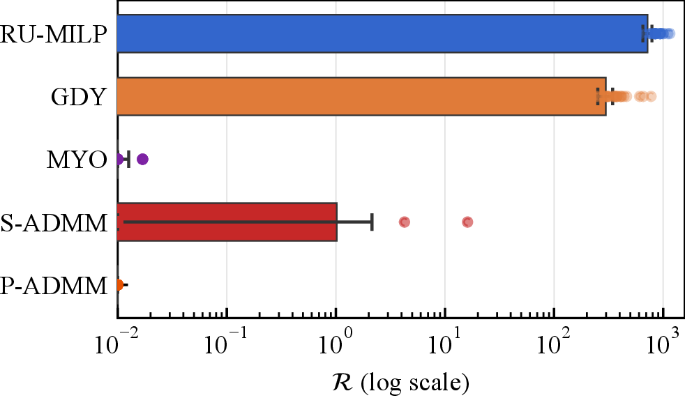
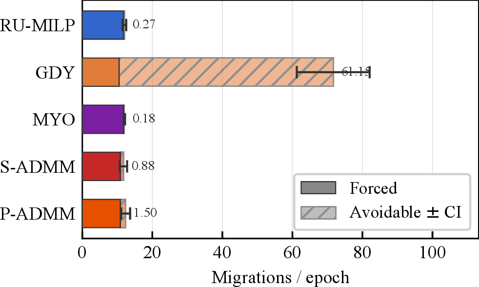
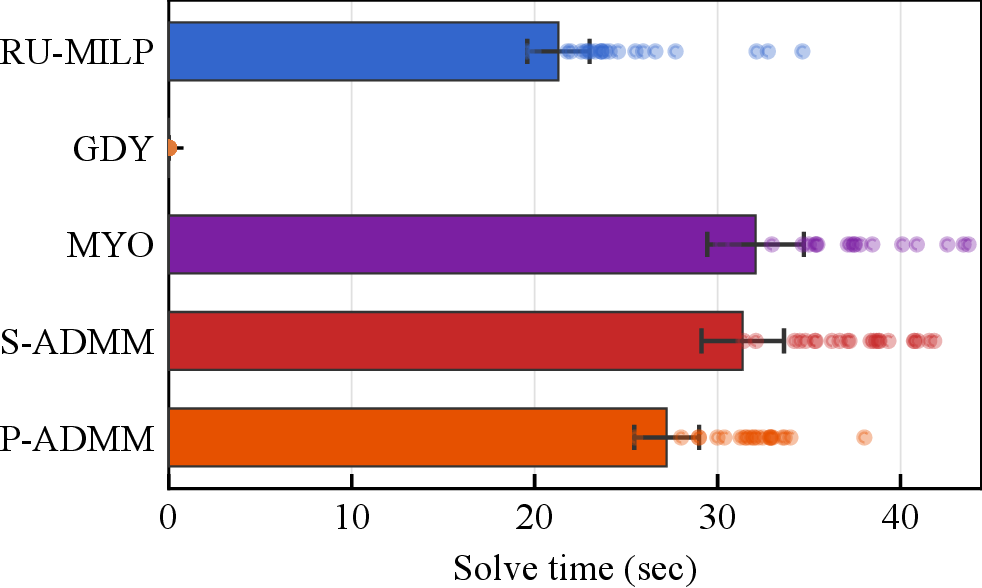
Figure 4: Average performance under the base configuration.. a — Average co-location risk \(\mathcal{R}\), b — Average migrations per epoch, c — Average solve time
Fig. 4 presents the average results, in terms of co-location risk, number of migrations per epoch, and solve time (in sec), of all five methods under the base configuration when \(N=10\). This is the largest slice count at which MYO remains solvable and thus the only setting admitting a direct five-method comparison across all performance dimensions.
Security co-location risk: Accorinding to Fig. 4 (a), MYO and P-admm eliminate co-location risk with \(\mathcal{R} = 0.005\) for MYO and \(\mathcal{R} = 0\) for P-admm, while S-admm reduces risk to \(\mathcal{R} = 1.02\). These security-aware methods stay three orders of magnitude below ru (\(\mathcal{R} = 720.2\)), confirming that ignoring the security term produces placements that regularly co-locate sensitive security vnf pairs as the workload grows. Finally, GDY achieves \(\mathcal{R} = 297.9\), which is lower than ru’s result since the geographic spread of sfcs provides sub-optimal incidental isolation.
Avoidable and forced VNF migrations: Based on Fig. 4 (b), where the avoidable portion of each bar is annotated with its numeric value so the small counts remain legible, MYO achieves an average of \(0.18\) avoidable migrations per epoch (hatched bars), while S-admm and P-admm incur \(0.88\) and \(1.50\), respectively. The per-slice decomposition of the proposed methods relaxes global continuity coordination, resulting in a slight increase in controllable churn relative to MYO. P-admm’s collision repair trades a small additional churn for tighter co-location separation. In contrast, ru retains prior assignments almost entirely, achieving near-zero avoidable migrations (\(0.27\) per epoch). At the opposite, GDY produces \(61.2\) avoidable migrations per epoch due to its epoch-by-epoch stateless reassignment. The forced migration rate is \(\approx 10.5\)–\(11.8\) per epoch for all milp-based methods, driven by topology-force handovers when a satellite drops below the elevation angle threshold.
Solve time: In Fig. 4 (c), the decomposed methods return a feasible placement on all trial-epoch samples, except for MYO, which fails on \(7\) of them in the base configuration. Specifically, MYO requires an average of \(32.1\),s per epoch across the \(33\) epochs for which it successfully converges; however, it exceeds the imposed solver time limit of \(300\),s in the remaining \(7\) epochs. P-admm achieves an average runtime of \(27.2\),s per epoch, making it approximately \(1.15\times\) faster than S-admm while maintaining greater reliability than MYO. In contrast, GDY and RU-milp exhibit significantly lower computational overhead. GDY completes execution almost instantaneously (\(\approx 0.01\),s per epoch) due to its single-pass BFS-based reassignment strategy, whereas RU-milp is the most computationally efficient milp formulation because it eliminates the \(O(N^2)\) co-location variables. Nevertheless, these computational gains come at the expense of substantially higher co-location risk, as illustrated in Fig. 4 (a). Consequently, the proposed decomposition-based approach offers the most computationally efficient security-aware solution, while remaining considerably more tractable than the joint milp formulation at \(N=10\).
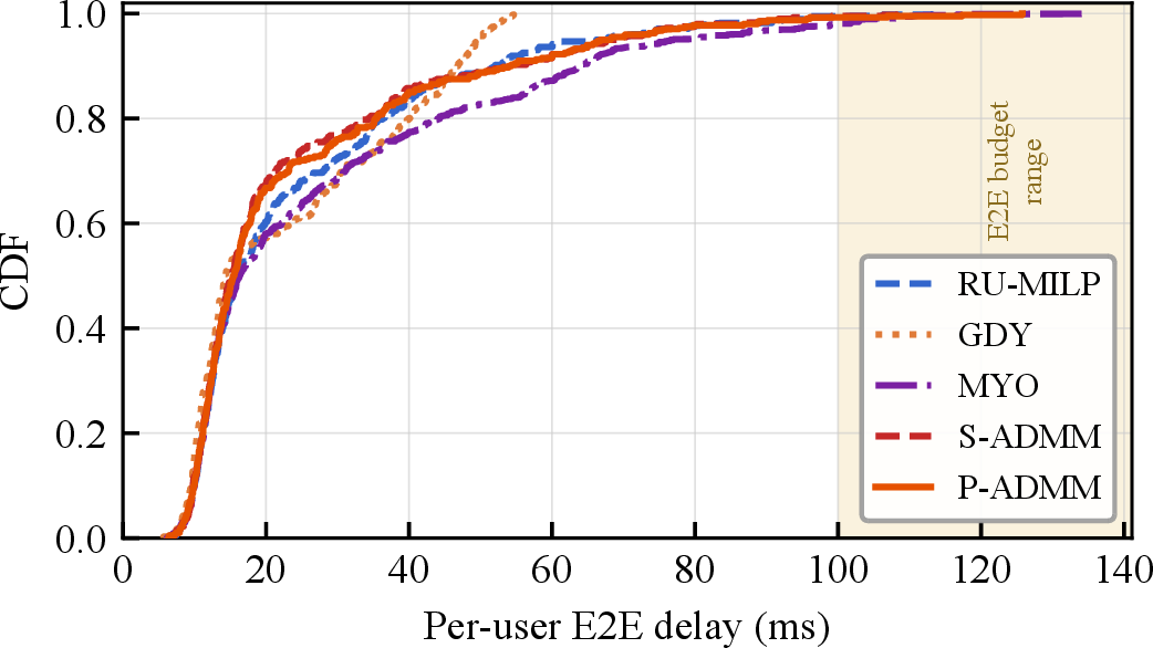
Delay distribution: Fig. 5 plots the cumulative distribution functions (CDFs) of the E2E delay of the compared methods. Accordingly, we see that every user’s E2E delay remains at or below \(135\) ms, which is within the defined delay thresholds \([100,150]\) ms. Nevertheless, almost all methods (except MYO) ensure that 100% of all users’ E2E delay is below 100 ms.
Epoch-by-epoch variability: Fig. 6 presents the per-epoch behaviours of risk and solve time over the \(20\) evaluation epochs. In the risk panel (Fig. 6 (a)), each plotted value is the average over the two random trials at that epoch index; the solve-time results are instead shown in a separate panel per trial (Figs. 6 (b) and 6 (c)), so that the epochs where MYO times out appear as breaks rather than being masked by trial averaging. Fig. 6 (a) shows that MYO, S-admm, and P-admm consistently maintain low risk across all epochs, while GDY and ru exhibit higher and more variable risk, due to the absence of security-aware objectives.
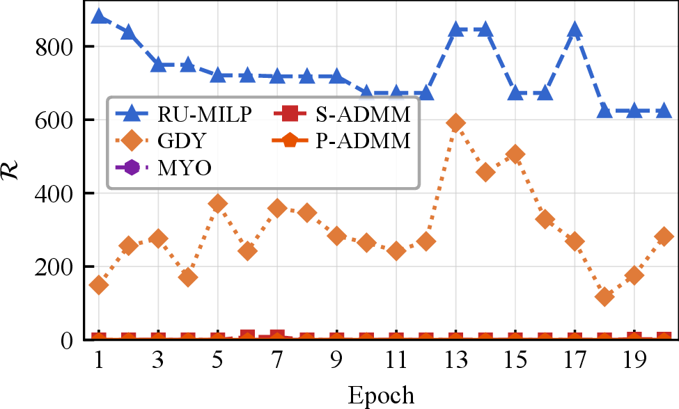
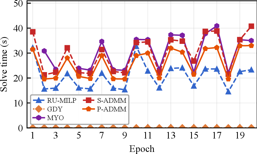
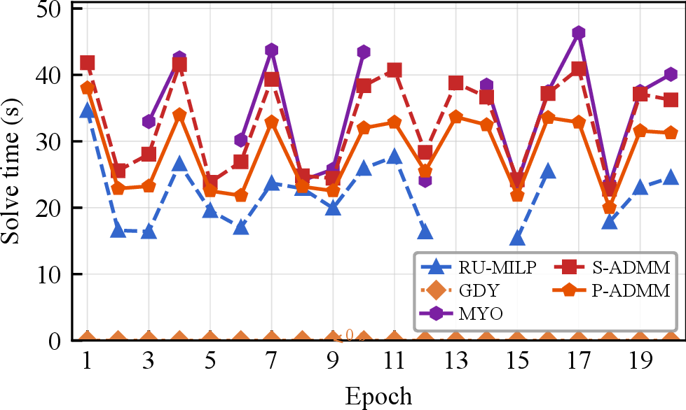
Figure 6: Per-epoch temporal dynamics: (a) security risk averaged over the two trials, and (b, c) solve time for each trial.. a — Per-epoch security risk (\(\mathcal{R}\)), b — Per-epoch solve time (trial 1), c — Per-epoch solve time (trial 2)
In Figs. 6 (b) and 6 (c), MYO returns a feasible solution on only \(33\) of \(40\) trial-epoch samples and times out on the remaining \(7\) (two in trial 1 and five in trial 2). Since each trial is drawn in its own panel, these timed-out epochs appear as breaks in MYO’s solid line, where no feasible solve time exists. For the other MILP methods, the solve times are in the range \([15,40]\) sec per epoch, with RU-MILP being the fastest solution. Nevertheless, the proposed ADMM methods achieve faster times than MYO, while ensuring that all epochs are resolved.
7.2 Scalability Analysis↩︎
In Fig. 7 , we present the averaged results, in terms of co-location risk, migrations per epoch, and solve time, for the considered methods, as functions of the number of slices \(N \in \{5,7,10,12,15,20,25\}\).
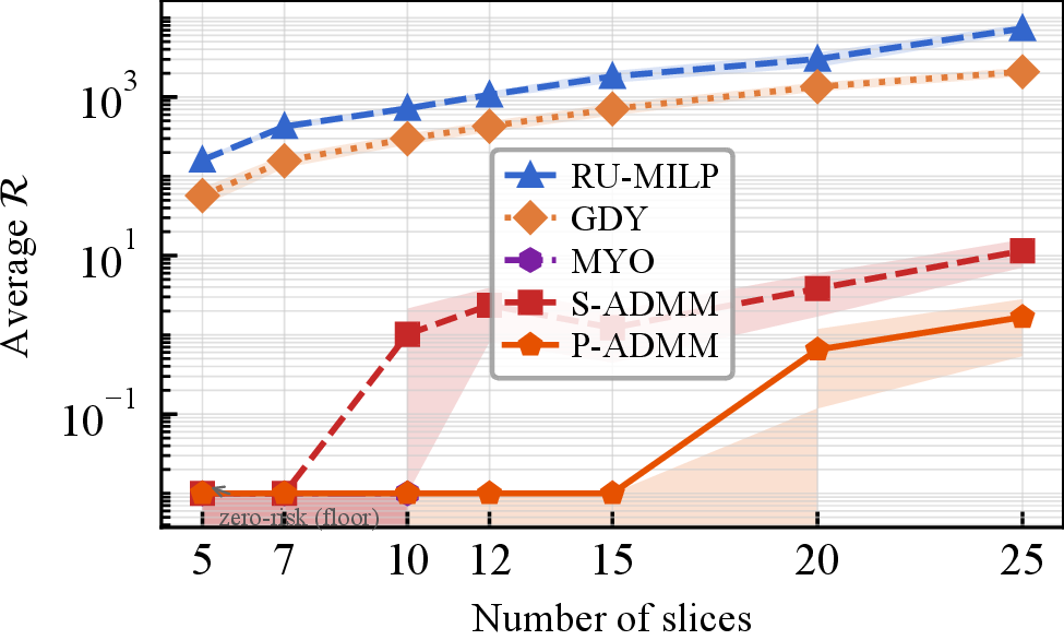
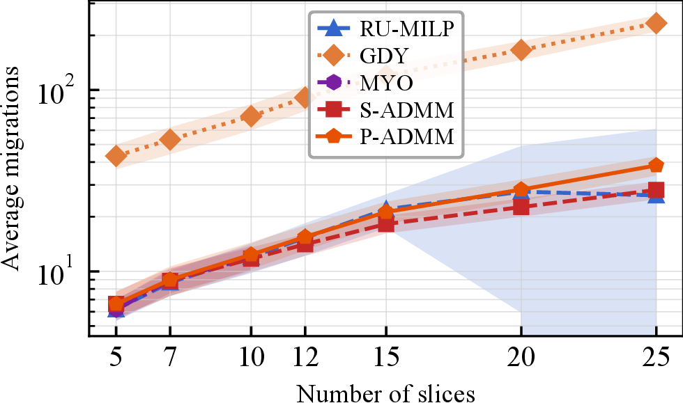
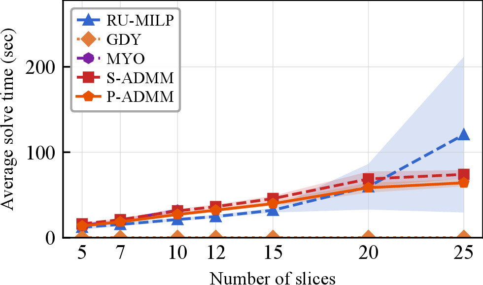
Figure 7: Scalability versus number of slices.. a — Log scaled average security risk (\(\mathcal{R}\)), b — Log scaled average migrations per epoch, c — Average solve time per epoch (s)
Security risk scaling: According to Fig. 7 (a), MYO reaches near-zero risk wherever feasible (\(N \leq 10\)), but collapses (no solution) for \(N>10\). In contrast, P-admm holds risk at exactly zero for \(N \leq 15\), with only a small residual (\(0.6\) at \(N=20\) and \(1.68\) at \(N = 25\)), as its deterministic repair separates every co-located pair that the \(I\) instances can handle. S-admm’s residual risk grows steadily (\(\mathcal{R} \in [1.02, 11.50]\) for \(N \in [10,25]\)) as the Gauss–Seidel updates fail under heavier coupling. Both admm methods remain orders of magnitude below the non-secure baselines, whose risk increases linearly (e.g., GDY reaches \(2084.6\) and ru \(7333\) for \(N = 25\)). ru’s feasibility also collapses for high \(N\) values, e.g., only \(4\) epochs were solved for \(N = 25\). Unlike MYO, ru omits the \(O(N^2)\) co-location variables. Hence, its infeasibility stems from the delay-constrained assignment, rather than co-location. Since unsolved epochs are the most contended, this feasible-only average understates ru’s true risk. In all panels of Fig. 7, the solid line is the mean over the trial-epoch samples and the shaded band is the \(95\%\) confidence interval of that mean.
Migration scaling: Based on Fig. 7 (b), the total number of migrations per epoch (the quantity plotted) scales linearly with \(N\) for MILP-based methods, consistent with a fixed topology-driven handover rate per epoch. S-admm keeps total migrations low and close to MYO, whereas P-admm consistently incurs more (e.g.\(38.4\) vs.\(28.1\) total migrations per epoch at \(N = 25\), and \(21.2\) vs.\(18.2\) at \(N = 15\)). The gap is driven by P-admm’s collision repair, which relocates additional instances to lower co-location risk, trading migration churn for tighter security; this is the risk-versus-migration trade-off that distinguishes the two schedules. As in Fig. 7, the shaded bands denote the \(95\%\) confidence interval of the per-epoch mean.
Solve time scaling: According to Fig. 7 (c), MYO’s solve cost grows steeply with \(N\) and exits the comparison beyond \(N = 10\) (cf.the feasibility limit noted above). P-ADMM and S-ADMM stay feasible on all \(40\) epochs at every scale and well within the \(120\) sec epoch budget, with mean solve times growing from \(16\) to \(74\) s for S-admm and \(14\) to \(64\) s for P-admm for \(N\) from \(5\) to \(25\). The security-unaware baselines bound the two extremes: GDY remains near-instantaneous at every \(N\), while RU-MILP is the cheapest milp but its solve time is reported over a shrinking feasible subset as its feasibility degrades at large \(N\) (e.g.\(4/40\) epochs at \(N = 25\)).
8 Conclusion↩︎
This paper addresses security- and migration-aware sfc placement in leo satellite constellations, where an epoch-by-epoch rotating topology couples confidentiality, service continuity, and computational tractability in ways absent from terrestrial nfv placement. The primary contribution is a unified placement framework built on two modelling advances: i) a co-location security risk model grounded in established ISO/NIST risk-management principles, equipped with analytic bounds that render cross-slice exposure a quantifiable optimization objective and ii) an avoidable-versus-forced migration formulation that penalizes only controllable churn against the unavoidable handover baseline imposed by orbital motion. These are cast as the first multi-slice security-aware single-epoch milp for leo sfc placement, subject to per-satellite CPU, isl, and per-user e2e delay constraints. To render this formulation deployable at practical slice counts, we employed an admm-style penalized per-slice best-response decomposition as the enabling solution technique. It transfers the quadratically growing cross-slice co-location coupling into a linear per-slice penalty. This decomposition replaces the intractable joint program with \(N\) independent subproblems coordinated through two complementary schedules: i) a sequential Gauss–Seidel refresh (S-admm) and ii) a parallel Jacobi schedule with deterministic collision repair (P-admm).
Evaluation over an \(80\)-satellite Walker–Delta constellation across a range of slice counts yields three principal insights. First, the decisive practical benefit is feasibility, as the framework returns a placement within the per-epoch time budget at every tested scale and sustains full e2e delay compliance. In contrast, the monolithic security-aware milp becomes intractable beyond a modest slice count. Therefore, the proposed framework operates precisely in the regime where the joint solver cannot. Second, embedding the risk model directly in the objective is what secures the placement. Both schedules suppress co-location risk by orders of magnitude relative to security-unaware optimization, with the parallel schedule holding risk at or near zero as the constellation scales. Third, the two schedules expose a controllable risk-versus-migration trade-off at a near-identical overall objective. The parallel schedule attains lower co-location risk for modestly more migration, while its independent schedule yields a secondary wall-clock speedup. Collectively, these results show that the proposed framework matches or exceeds the security of the joint optimum while scaling to operating regimes that the monolithic formulation cannot reach.
Some limitations delineate the scope of these findings and motivate future work. The decomposition guarantees a monotone, bounded incumbent and a coordinate-wise best-response equilibrium at its fixed point (Proposition 2) rather than convergence to the joint optimum. Additionally, the realized parallel speedup is bounded by a thread-based implementation in which only the per-slice solver calls execute concurrently. Building on this foundation, future work includes a predictive multi-epoch extension that pre-positions vnfs across orbital handoffs, a process-parallel or distributed implementation that realizes the decomposition’s full speedup, and validation across heterogeneous multi-orbit configurations. By making cross-slice co-location risk a quantifiable and tractable objective, this framework provides a tractable basis for secure, continuity-aware service orchestration as on-orbit edge computing scales toward 6G deployment.