Search-Based Spatiotemporal and Multi-Robot Motion Planning on Graphs of Space-Time Convex Sets
July 01, 2026
Abstract
Spatiotemporal motion planning, especially in multi-robot settings, requires robots to reason about collision-free regions that change over time, which is challenging in continuous spaces when feasible regions are transient and geometrically constrained. We present an algorithmic framework based on graphs of space-time convex sets (ST-GCSs), where collision-free regions are represented as convex sets in space-time and trajectories correspond to paths on the graph together with continuous motions within the selected sets. We formulate time-optimal planning on ST-GCSs as a graph-search problem over path-indexed states and develop a best-first search solver that evaluates partial paths via continuous trajectory optimization, guided by admissible heuristics and dominance checks. We further present an Exact Convex Decomposition (ECD) scheme to reserve trajectory occupancies in space-time, enabling unified handling of dynamic obstacles and multi-robot interactions. For multi-robot motion planning, we integrate ST-GCS planning and ECD into prioritized planning methods and introduce a windowed coordination scheme to improve efficiency. Extensive experiments on single-robot and multi-robot problems demonstrate substantial speedups over various planners while maintaining high solution quality, particularly in environments with narrow and transient feasible regions. Large-scale demonstrations further show that the proposed multi-robot motion planner can solve instances with up to \(100\) robots within only a few minutes. Project homepage: https://sites.google.com/view/stgcs.
Keywords: Motion Planning, Multi-Robot Coordination, Heuristic Search, Graphs of Convex Sets
1 Introduction↩︎
Spatiotemporal motion planning is a core problem in robotics. A robot must move from a start state to a goal while avoiding both static obstacles and time-varying constraints induced by dynamic environments or other robots. This problem becomes particularly challenging in continuous domains when feasible regions are transient, geometrically constrained, and tightly coupled with time. Such conditions arise naturally in Multi-Robot Motion Planning (MRMP), where each robot must treat the trajectories of others as dynamic obstacles, as well as in single-robot planning tasks with moving obstacles or temporal constraints.
Despite extensive progress, existing approaches still struggle to provide efficient and reliable solutions in these settings. Sampling-based planners, such as PRM [1] and RRT [2], and their spatiotemporal variants [3], [4], offer modeling flexibility but rely on random exploration, which can be ineffective in capturing narrow or short-lived feasible regions in space-time. Their performance further degrades due to repeated collision checking in a time-augmented state space. Optimization-based approaches based on the Graph of Convex Sets (GCS) replace random exploration with deterministic reasoning over convex decompositions [5], [6], but extending them to dynamic environments requires a unified treatment of time, velocity constraints, and dynamic obstacle avoidance. When formulated as a single large optimization, this leads to significant computational challenges.
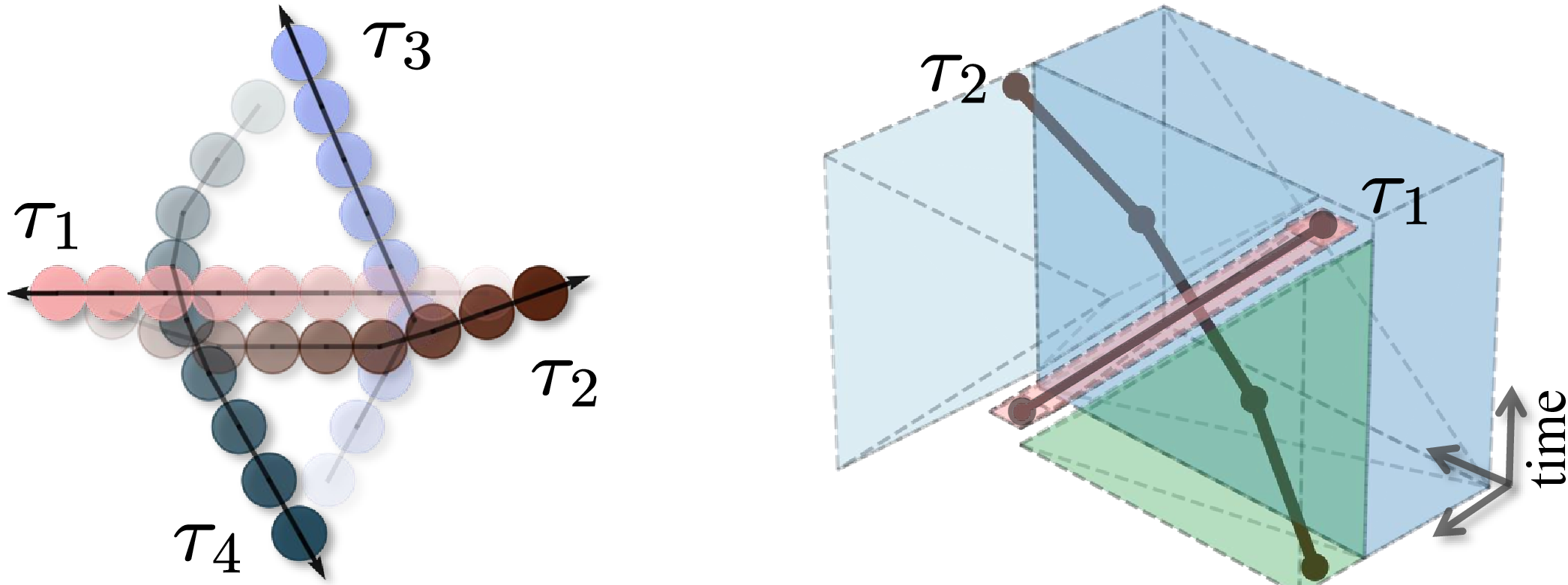
In this work, we present a general framework for time-optimal spatiotemporal motion planning in continuous spaces with dynamic obstacles based on a novel graph representation, namely a Graph of Space-Time Convex Sets (ST-GCS), where vertices correspond to collision-free convex sets in space-time and edges encode nonempty intersections between sets. An ST-GCS extends a spatial GCS into the time dimension, allowing both geometric and temporal constraints to be captured within a single graph structure. A feasible trajectory then corresponds to a path on an ST-GCS together with a continuous trajectory constructed within the selected convex sets. This representation also provides a natural basis for spatiotemporal planning in dynamic environments and for multi-robot coordination, where planned robot trajectories can be incorporated back into the graph as reserved occupancies.
A key challenge in solving time-optimal planning on an ST-GCS by graph search is that the cost and feasibility of reaching a vertex cannot be determined solely by the vertex itself. Instead, they depend on the entire prefix path used to reach that vertex, since different paths induce different feasible arrival states and different continuation costs. As a result, standard shortest-path formulations that identify search states only by vertices are generally insufficient. To address this, we formulate planning on an ST-GCS as a graph search over path-indexed states, where each search node represents a partial path together with the corresponding optimal trajectory and its cost.
Building on this formulation, we develop a best-first search solver for planning on ST-GCSs and introduce several algorithmic components that together make it practical and scalable. The search repeatedly evaluates partial paths by solving the corresponding continuous trajectory optimization over the convex sets along that path. To improve efficiency, we design admissible heuristics over partial paths and develop reachability-based dominance checks, including a safe set-containment check that preserves optimality and two lightweight heuristic checks that are substantially faster while maintaining high solution quality in practice. In addition, we present the Exact Convex Decomposition (ECD) scheme to reserve the spatiotemporal occupancy of trajectories by updating an ST-GCS, thereby enabling a unified treatment of dynamic obstacles and inter-robot interactions. On top of this, we integrate ECD into prioritized planning methods for MRMP, and further introduce a windowed coordination scheme to improve efficiency in multi-robot coordination by focusing planning effort on the relevant time intervals. We demonstrate the proposed Windowed-PBS + BFS planner on large-scale and highly congested MRMP instances, solving a bottlenecked \(50\)-robot instance in \(1.64\)m and a dense \(100\)-robot instance in \(1.60\)m, which shows its scalability beyond the main benchmark range.
We summarize our contributions as follows:
We formulate time-optimal spatiotemporal motion planning as a graph-search problem on ST-GCSs.
We develop a search-based solver that operates on path-indexed states, together with admissible heuristics and dominance checks tailored to searching ST-GCSs.
We present the ECD scheme to reserve trajectory occupancies in arbitrary-dimensional space-time, enabling unified handling of dynamic obstacles and multi-robot interactions.
We integrate ST-GCS planning and ECD into prioritized planning methods for MRMP, and further introduce a windowed coordination scheme to improve efficiency in multi-robot coordination.
We provide extensive empirical evaluation demonstrating substantial speedups over optimization-based approaches and strong performance in challenging spatiotemporal scenarios.
This work substantially extends our prior conference version [7] as follows:
The prior version formulates time-optimal motion planning on an ST-GCS as a unified optimization problem, whereas this work develops a search-based formulation on ST-GCSs with path-indexed states, pruning strategies, and heuristic guidance, resulting in orders of magnitude faster in practice.
The prior version presents ECD in the original 3D setting arising from 2D spatial motion plus time, whereas this work generalizes ECD to arbitrary-dimensional space-time.
The prior version integrates ST-GCS within prioritized multi-robot planning, whereas this work additionally introduces windowed coordination to improve efficiency in multi-robot coordination.
This work also provides substantially more extensive empirical evaluation, including additional search ablations and real-robot experiments.
2 Related Work↩︎
This section positions our work relative to spatiotemporal planning, MRMP, and planning on GCSs.
2.1 Spatiotemporal Motion Planning↩︎
Spatiotemporal motion planning treats time as part of the planning domain to handle moving obstacles with known trajectories [8]. Grid-based methods reserve discrete space-time states [9]; SIPP reasons over safe time intervals for discrete spatial occupancies [10]; any-angle variants such as Zeta\(^*\)-SIPP combine safe intervals with any-angle search for time-optimal planning in dynamic environments [11]; and state-lattice methods plan over spatiotemporal lattices built from continuous space and fixed motion primitives [12]. Sampling-based planners lift RRT-, PRM-, and RRT\(^*\)-style methods into configuration–time space, validating sampled time-parameterized states or edges against moving obstacles over their execution intervals [3], [4], [13]; they are flexible, but can struggle when feasible regions are narrow, short-lived, or repeatedly changing, and their runtime can be dominated by collision checking in the time-augmented state space. Recent work mitigates this issue by bringing safe-interval ideas from MAPF [10] into sampling-based planning [14], [15]. In contrast, we plan on ST-GCSs: collision-free space-time is represented by convex sets connected through nonempty intersections, so reserved occupancies can be removed from an updatable free-space decomposition while continuous trajectory optimization remains available over remaining regions.
2.2 MRMP↩︎
MRMP methods differ mainly in how they represent and resolve inter-robot conflicts. Coupled methods reason in composite configuration spaces. Coordinated PRMs explicitly construct products of individual roadmaps [16], dRRT-style methods explore implicit tensor-product roadmaps without materializing the full joint graph [17], [18], and partially coupled methods such as M\(^*\) plan independently when possible while expanding into higher-dimensional coupled search near conflicts [19]. Decoupled and conflict-based methods improve scalability by using priorities, reservations, or constraints. Prioritized planning treats planned robots as moving obstacles in configuration–time space [8], [20], cooperative pathfinding uses discrete space-time reservations [9], CBS separates high-level conflict resolution from low-level planning [21], and PBS searches over priority constraints rather than a fixed ordering [22]. These ideas underlie MAPF variants including continuous-time MAPF [23], safe-interval planning on continuous-time roadmaps [24], and representation-optimal MRMP for heterogeneous robots in continuous spaces [25].
Recent MRMP work connects conflict-based coordination with sampling-based, kinodynamic, optimization, and control-based planning. Kinodynamic CBS incorporates motion primitives into CBS [26], while adaptive methods vary coupling online through adaptive robot coordination [27], kinodynamic adaptive coordination [28], or guidance-informed grouping [29]. Other approaches use decentralized trajectory optimization [30], path retiming [31], CBS-guided MPC [32], or mixed-integer continuous formulations [33], [34]. Our MRMP planner is closest to prioritized planning, but each low-level query plans on an ST-GCS; after a robot is planned, ECD updates the ST-GCS to reserve its swept occupancy, so later robots plan in the remaining collision-free space-time and jointly reason about route choice, timing, and dynamic collision avoidance.
2.3 Planning on GCSs↩︎
GCSs combine graph structure with convex optimization for mixed discrete–continuous planning [5], [6]. They have been applied beyond cluttered Euclidean motion planning to non-Euclidean configuration spaces [35], temporal-logic and precedence-constrained planning [36], [37], contact-rich manipulation [38], and guidance for downstream nonconvex trajectory optimization [39]. These works demonstrate the breadth of GCS modeling, but mainly consider static, task-augmented, or contact-mode domains rather than a free-space representation repeatedly updated by moving obstacles and planned robot trajectories.
GCS performance depends strongly on the convex decomposition of free space. IRIS grows large obstacle-free convex regions [40]; visibility-graph clique covers and certified polyhedral decompositions improve coverage, certification, and scalability [41], [42]; and GPU-accelerated methods compute collision-free configuration-space convex sets online in changing environments [43]. Our ECD scheme is complementary. It updates an ST-GCS by removing swept occupancies while maintaining a convex decomposition of the remaining collision-free space-time.
Efficient GCS solving has also received substantial attention. Large safe-box planners exploit offline preprocessing with fast runtime shortest-path and convex-control subproblems [44], while search-based solvers such as GCS\(^*\) [45], implicit graph search [46], and A\(^*\)-GCS [47] reduce reliance on one monolithic mixed-integer convex program over the full graph. Other variants address multi-query planning [48], shortest walks with repeated vertices [49], nonconvex-cost [50] or parametrized-space objectives [51], fixed-sequence minimum-time motion through convex sets [52], and routing problems that couple discrete visitation order with continuous trajectories [53]–[55]. Closest to our setting, [56] studies ST-GCS planning in dynamic environments and constructs GCS-compatible constraints, while [57] combines CBS with time-augmented GCS under a fixed time-step representation. Recent GCS work has expanded modeling scope and solver efficiency, but has not jointly addressed path-indexed search on ST-GCSs, occupancy reservation by convex-decomposition updates, and windowed multi-robot coordination.
3 Preliminaries↩︎
This section introduces the notation and basic GCS formulation used in this paper. We first review the standard definition of (spatial) GCSs, where vertices correspond to collision-free convex sets and edges indicate nonempty intersections. We then describe the standard motion-planning problem on GCSs and the path-conditioned convex subproblem used later by our search-based solver for planning on ST-GCSs.
3.1 GCS Definition↩︎
We consider a robot with an \(m\)-dimensional state space, whose collision-free region is decomposed into a collection of convex sets. These spatial convex sets need not be disjoint. A GCS, denoted as \(G=(V, E, \mathcal{X})\), is a connected graph representing such a convex decomposition, where \(V\) is the vertex set, \(E\) is the edge set, and \(\mathcal{X}=\{X_v\}_{v\in V}\) is the collection of convex sets. Each vertex \(v\in V\) corresponds to a convex set \(X_v =\{\mathbf{x}\,|\,\mathbf{A}_v\mathbf{x}\preceq \mathbf{b}_v\}\subseteq\mathbb{R}^m\) of states. Each edge \(e=(u,v)\in E\) indicates that \(X_u\cap X_v\neq\emptyset\). Our use of GCS is slightly more restrictive than the original formulation of [6], where constraints may be attached more generally to vertices and edges.
A path on \(G\) is an ordered sequence of vertices \(\pi=\langle v_1,v_2,\ldots,v_{l} \rangle\) where \((v_{i-1},v_i)\in E\) for all \(i=2,\ldots,l\). Unless otherwise stated, we consider simple paths, i.e., paths without repeated vertices. A trajectory associated with \(\pi\) is a continuous curve obtained by concatenating local trajectory segments inside the convex sets along \(\pi\).
3.2 Motion Planning on GCSs↩︎
Given a start state \(\mathbf{x}_s\) and a goal state \(\mathbf{x}_g\), motion planning on a GCS \(G=(V,E,\mathcal{X})\) asks for a trajectory from \(\mathbf{x}_s\) to \(\mathbf{x}_g\). Since the start and goal states may lie in multiple convex sets, we introduce auxiliary source and target vertices \(v_s\) and \(v_g\), with \(X_{v_s}=\{\mathbf{x}_s\}\) and \(X_{v_g}=\{\mathbf{x}_g\}\), connected to all start- and goal-containing vertices, respectively, and use these auxiliary vertices as the unique endpoints of the graph path. We introduce two sets of variables. The binary edge-selection variables \(\Phi=\{\phi_e\}_{e\in E}\) parameterize a path \(\pi_\Phi\), where \(\phi_e=1\) if and only if edge \(e\) is selected by the path \(\pi_\Phi\). The continuous variables \(\mathbf{x}_{v}, \mathbf{y}_{v}\in X_v\) represent the entry and exit states of the local trajectory segment inside \(X_v\). For each vertex \(v\in V\), let \(\ell_v(\mathbf{x}_v,\mathbf{y}_v)\) denote a given local cost associated with vertex \(v\). The motion planning problem on GCS can be written as: \[\begin{align} \min_{\Phi,\mathbf{x},\mathbf{y}}\; & \sum_{v\in \pi_\Phi} \ell_v(\mathbf{x}_v,\mathbf{y}_v)\tag{1}\\ \boldsymbol{s.t.}\; & \pi_\Phi = \langle v_s,\ldots,v_g \rangle \in \mathcal{P}(v_s, v_g;G),\tag{2}\\ &\mathbf{x}_v, \mathbf{y}_v\in X_v,&\makebox[36pt][r]{\forall v\in \pi_\Phi,}\tag{3}\\ &\mathbf{x}_v=\mathbf{y}_u,&\makebox[36pt][r]{\forall (u,v)\in E(\pi_\Phi),}\tag{4}\\ &\mathbf{x}_{v_s}=\mathbf{x}_s\text{ and }\mathbf{y}_{v_g}=\mathbf{x}_g,\tag{5} \end{align}\] where \(\mathcal{P}(v_s, v_g;G)\) denotes the set of simple paths in \(G\) that start from \(v_s\) and end at \(v_g\).
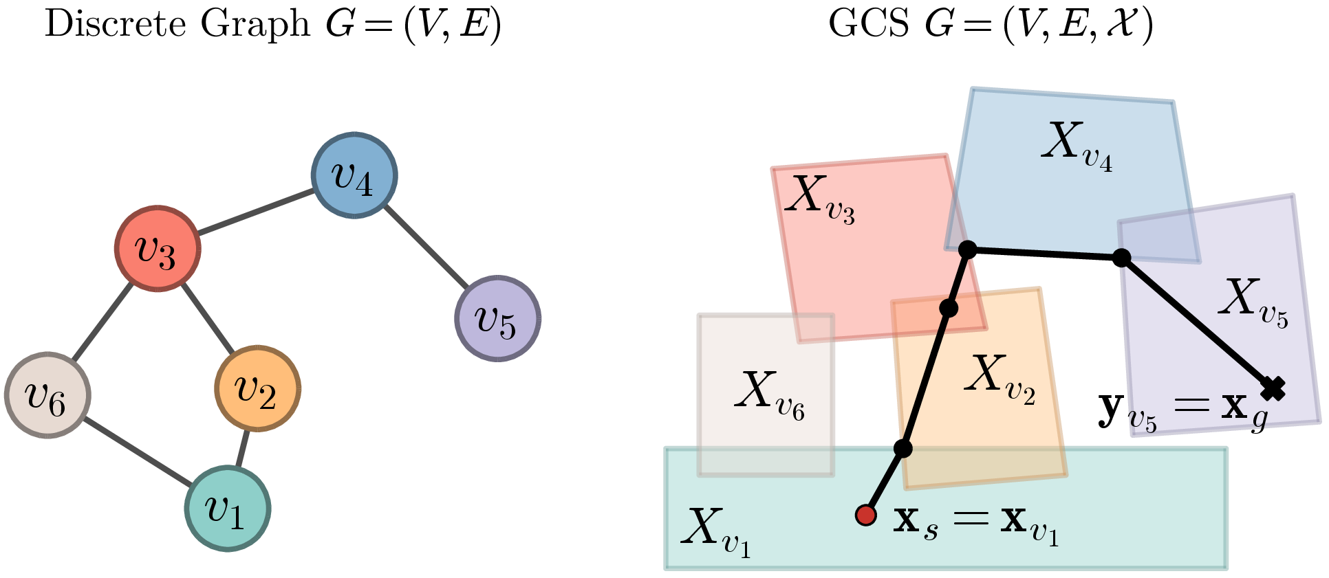
The objective in Eqn. (1 ) sums the local costs of the trajectory segments \(\mathbf{x}_v \rightarrow \mathbf{y}_v\) along the selected path. Eqn. (2 ) enforces that the selected edges form a valid simple path from the auxiliary source vertex to the auxiliary target vertex. This path constraint can be encoded using standard flow-conservation and degree constraints for routing problems [58], [59], yielding a Mixed-Integer Convex Program (MICP). Eqn. (3 ) enforces that each local segment lies inside the corresponding convex set. Since \(X_v\) is convex, the straight-line segment \((\mathbf{x}_v,\mathbf{y}_v)\) is collision-free. Eqn. (4 ) enforces continuity between consecutive local segments for every selected edge. Eqn. (5 ) enforces the trajectory starts from and ends at the given start state and goal state, respectively.
As illustrated in Fig. 2, a feasible solution reconstructs a continuous, collision-free, piecewise-linear trajectory from \(\mathbf{x}_s\) to \(\mathbf{x}_g\) by chaining the local segments \(\mathbf{x}_v \rightarrow\mathbf{y}_v\) along \(v\in\pi_\Phi\). The above formulation focuses on kinematic feasibility, which aligns with the standard convention in the literature. Differential or kinodynamic constraints can be incorporated by augmenting the state space and adding suitable constraints, such as in [5]. The formulation can also be adapted to a convex start set \(X_s\) or a convex goal set \(X_g\) by replacing the point constraints in Eqn. (5 ) with set-membership constraints.
3.3 Path-Conditioned Optimization↩︎
Solving Eqns. (1 –5 ) directly as an MICP can be computationally expensive [6]. A useful subproblem is obtained by fixing the graph path and optimizing only the continuous variables along that path. This operation is commonly referred to as convex restriction [60] and is used as a subroutine in several search-based solvers for graph optimization problems on GCSs [46], [55], [61].
Given a path \(\pi=\langle v_1,v_2,\ldots,v_l \rangle\) on \(G\), we say that a trajectory \(\tau\) is conditioned on \(\pi\) if it is represented by an ordered sequence \(\tau=\langle(\mathbf{x}_{v_i},\mathbf{y}_{v_i})\rangle_{i=1}^l\) of entry and exit states, where \(\mathbf{x}_{v_i},\mathbf{y}_{v_i}\in X_{v_i}\) with continuity enforced between consecutive sets. Conditioning on a path \(\pi\) fixes the binary variables \(\Phi\) so that \(\pi_\Phi = \pi\). The remaining optimization is the convex program over the continuous entry and exit states, given as follows: \[\begin{align} \min_{\mathbf{x},\mathbf{y}}\quad & \sum_{i=1}^l \ell_{v_i}(\mathbf{x}_{v_i},\mathbf{y}_{v_i})\\ \boldsymbol{s.t.}\quad &\mathbf{x}_{v_i},\mathbf{y}_{v_i}\in X_{v_i},&i=1,\ldots,l,\\ &\mathbf{x}_{v_i}=\mathbf{y}_{v_{i-1}},&i=2,\ldots,l,\\ &\mathbf{x}_{v_1}=\mathbf{x}_s\text{ and }\mathbf{y}_{v_l}=\mathbf{x}_g. \end{align}\] This is a convex program that off-the-shelf optimizers can efficiently solve whenever the local costs and set constraints are convex. If feasible, its solution defines the optimal trajectory conditioned on the fixed path \(\pi\). For example, in Fig. 2, fixing \(\pi=\langle v_1,v_2,v_3,v_4,v_5 \rangle\) removes the discrete path-selection variables and optimizes only the entry and exit state variables along that path.
4 Spatiotemporal Planning on ST-GCSs↩︎
This section extends the GCS formulation in Sec. 3 to spatiotemporal motion planning. The key concept is a Graph of Space-Time Convex Sets (ST-GCS), where each convex set lies in the joint space of position and time. Planning on an ST-GCS allows dynamic-obstacle avoidance, variable arrival times, velocity limits, and time optimality to be handled within a unified graph-optimization problem.
4.1 Problem Formulation↩︎
Let \(G=(V, E, \mathcal{X})\) denote an input ST-GCS, where \(\mathcal{X}=\{X_v\}_{v\in V}\) is a collection of space-time convex sets. Each vertex \(v\in V\) corresponds to a space-time convex set \(X_v\subset\mathbb{R}^{m+1}\) that is collision-free from both static and dynamic obstacles. Each edge \((u,v)\in E\) indicates that \(X_u\cap X_v\neq\emptyset\). As shown in Fig. 3, an ST-GCS can be initialized by extruding each given spatial collision-free convex set from time \(0\) to an arbitrarily large but finite time limit \(t_{\text{max}}\). In addition, the ECD scheme introduced in Sec. 6 can further remove the space-time occupancies of dynamic obstacles or previously planned robots, potentially subdividing the extruded sets.
![Figure 3: A 3D ST-GCS (right) constructed by extruding each set of a 2D spatial GCS (left) along the time dimension t \in[0, t_{\max}]. A feasible trajectory is planned from the start state \mathbf{x}_s to the goal position \mathbf{p}_g, with the dashed vertical line indicating the possible goal states \mathbf{x}_g=(\mathbf{p}_g,t) across time.](/article/2607.00444/figs/stgcs.png "fig:")
Let \(\mathbf{x}=(\mathbf{p},t)\in\mathbb{R}^{m+1}\) denote a space-time state, where \(\mathbf{x}.\mathbf{p}\in\mathbb{R}^m\) is the spatial position and \(\mathbf{x}.t\in\mathbb{R}\) is the time. Within each space-time convex set \(X_v\), the local trajectory segment \(\mathbf{x}_v \rightarrow \mathbf{y}_v\) is linear in space-time, that is, traversed at a uniform speed but may vary across different sets. For each \(v\), we let \(\Delta t_v= \mathbf{y}_v.t-\mathbf{x}_v.t\) and \(\Delta \mathbf{p}_v= \mathbf{y}_v.\mathbf{p}-\mathbf{x}_v.\mathbf{p}\) denote the elapsed time and spatial displacement of the segment within \(X_v\), respectively.
For each query, we consider a start space-time state \(\mathbf{x}_s\) and a goal spatial position \(\mathbf{p}_g\), with an unconstrained arrival time. To avoid treating multiple start- or goal-containing vertices specially, we augment \(G\) with a single auxiliary start vertex \(v_s\) and a single auxiliary goal vertex \(v_g\) [59]. In this work, we consider a single start state point \(\mathbf{x}_s\) and define: \[X_{v_s}=\{\mathbf{x}_s\}.\] More generally, \(X_{v_s}\) can be any convex set of admissible start states. The auxiliary goal set contains all admissible goal states induced by \(\mathbf{p}_g\). In this work, by convention, a solution must also allow the robot to remain at \(\mathbf{p}_g\) after arrival until the time limit \(t_\text{max}\). We therefore define the auxiliary goal set by \[\begin{align} X_{v_g} = \Big\{&(\mathbf{p}_g,t)\Bigm\vert 0\leq t\leq t_{\max} \text{ and }\\ &(\mathbf{p}_g,t')\in \bigcup_{v\in V}X_v\;\text{for all } t'\in[t,t_{\max}]\Big\}. \end{align}\] Thus, membership in \(X_{v_g}\) certifies that the robot reaches \(\mathbf{p}_g\) at a time from which it can safely remain there until \(t_{\max}\) through the space-time collision-free region \(\bigcup_{v\in V}X_v\) represented by \(G\). If the query instead specifies a full goal state, or only requires reaching \(\mathbf{p}_g\) without remaining there, the definition of \(X_{v_g}\) can be modified directly while the rest of the formulation remains unchanged. We define the query-augmented ST-GCS as \(G^\sharp=(V^\sharp,E^\sharp,\mathcal{X}^\sharp)\), where \(V^\sharp=V\cup\{v_s,v_g\}\), \(\mathcal{X}^\sharp=\mathcal{X}\cup\{X_{v_s},X_{v_g}\}\), and \(E^\sharp = \{(u,v)\mid u,v \in V^\sharp, u\neq v, X_u \cap X_v \neq \emptyset\}\). We denote this construction by \((G^\sharp,v_s,v_g)=\mathrm{\small QueryAugment}(G,\mathbf{x}_s,\mathbf{p}_g)\). Fig. 4 illustrates a query-augmented ST-GCS.
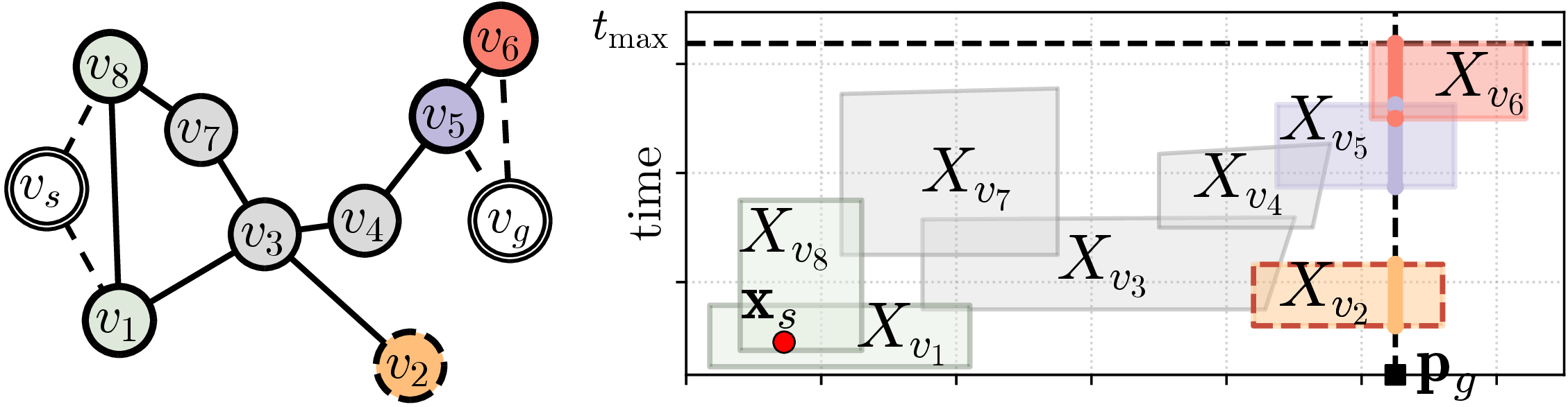
Given a component-wise velocity bound \(\mathbf{v}_{\mathrm{lim}}\in \mathbb{R}^{m}_{>0}\), the time-optimal spatiotemporal planning problem on the query-augmented ST-GCS \(G^\sharp\) is written as: \[\tag{6} \begin{align} \min_{\Phi,\mathbf{x},\mathbf{y}}\quad & c(\tau)=\sum_{v\in\pi_\Phi}\Delta t_v\tag{7}\\ \boldsymbol{s.t.}\quad &\pi_\Phi\in \mathcal{P}(v_s,v_g;G^\sharp),\tag{8}\\ &\mathbf{x}_v,\mathbf{y}_v\in X_v, &&\forall v\in\pi_\Phi,\tag{9}\\ &\mathbf{x}_v=\mathbf{y}_u, &&\makebox[36pt][r]{\forall (u,v)\in E^\sharp(\pi_\Phi),}\tag{10}\\ &\Delta t_v \geq 0, &&\forall v\in\pi_\Phi,\tag{11}\\ &-\mathbf{v}_{\mathrm{lim}}\Delta t_v \preceq \Delta \mathbf{p}_v\preceq \mathbf{v}_{\mathrm{lim}}\Delta t_v, &&\forall v\in\pi_\Phi.\tag{12} \end{align}\] Eqn. (7 ) minimizes the time cost \(c(\tau)\), defined as the total elapsed time of trajectory \(\tau\) reconstructed from the selected path \(\pi_\Phi\) and continuous variables. Eqns. (8 –10 ) folllow the graph topology, set membership, and continuity constraints from Eqns. (2 –4 ), specialized to the query-augmented ST-GCS \(G^\sharp\). Eqn. (11 ) enforces time monotonicity within each selected convex set. Eqn. (12 ) imposes component-wise velocity limits by bounding spatial displacement over elapsed time within each selected convex set. The auxiliary start and goal vertices encode the query through set membership and graph connectivity. Since \(X_{v_s}=\{\mathbf{x}_s\}\), the trajectory starts at \(\mathbf{x}_s\). Since \(X_{v_g}\) contains only states with spatial position \(\mathbf{p}_g\), any feasible path ending at \(v_g\) reaches the goal position. Under the goal-staying convention, membership in \(X_{v_g}\) further guarantees that the robot can remain at \(\mathbf{p}_g\) until \(t_{\max}\). As illustrated in Fig. 3, a feasible solution reconstructs a continuous, space-time collision-free, piecewise-linear trajectory \(\tau\) from \(\mathbf{x}_s\) to some goal state \(\mathbf{x}_g=(\mathbf{p}_g,\cdot)\).
4.2 Optimization-Based Solving↩︎
The formulation above can be solved as an MICP. The binary variables select a sequence of space-time convex sets, while the continuous variables optimize the entry and exit states within the selected sets. Time monotonicity, velocity limits, and continuity between consecutive local trajectory segments constrain these continuous states.
Following [7], we use two optimization-based variants as baselines in our experiments. The first, denoted by MICP, solves the mixed-integer program directly. The second, denoted by MICP(g), solves the continuous relaxation and then applies stochastic path rounding multiple times. Once a graph path is fixed, the remaining trajectory optimization is path-conditioned, as described in Sec. 3.3.
5 Graph Search on ST-GCSs↩︎
This section presents the search-based solver for spatiotemporal planning on ST-GCSs. We first define the path-indexed search space and explain why vertex-indexed shortest-path search is insufficient. We then justify excluding set revisitation under the piecewise-linear trajectory representation. Finally, we describe the best-first search solver, which repeatedly solves path-conditioned convex programs, uses admissible heuristics for guidance, and applies upper-bound pruning and dominance checks for pruning the search tree.
5.1 Search Space↩︎
In standard cost-minimal-path search on a discrete graph, such as A\(^*\) search [62], a search state is typically identified by the current vertex. This is valid because the graph has a vertex-level optimal substructure. Once the minimum cost-to-come to a vertex \(v\) is known, any more expensive prefix ending at \(v\) can be discarded, since all future costs depend only on \(v\) and the remaining path.
This vertex-level optimal substructure does not generally hold for motion planning on GCSs or ST-GCSs. The cost of a path is not the sum of fixed edge costs. Instead, once a vertex sequence is chosen, the continuous trajectory variables along the entire sequence are optimized jointly. Consequently, when a prefix path \(\pi = \langle v_s,\ldots,v \rangle\) is extended to \(\pi'= \langle v_s,\ldots,v,w \rangle\), the optimal continuous states along the earlier part of the path, including the state at \(v\), may change. Thus, the optimal trajectory conditioned on \(\pi'\) is not obtained by simply appending a locally optimal transition from \(v\) to \(w\) to the optimal trajectory conditioned on \(\pi\). A prefix that is more expensive when considered only up to \(v\) may still result in a lower-cost full trajectory after extension.
Thus, search nodes for planning on ST-GCSs must be indexed by the full prefix path, rather than only by the arrival vertex. Let \(\Pi\) denote the set of partial vertex paths on the query-augmented \(G^\sharp\) that start from the auxiliary start vertex \(v_s\). As justified in Sec. 5.2, we restrict \(\Pi\) to paths that do not revisit a vertex.
Definition 1 (Path-Indexed Search Node). A search node, identified by its prefix path, is a record \[N=(\pi,v,\tau,g,f),\] where \(N.\pi \in \Pi\) is the prefix path, \(N.v\) is the last vertex of \(N.\pi\), \(N.\tau\) is the optimal trajectory conditioned on \(N.\pi\), \(N.g = c(N.\tau)\) is the cost-to-come, and \(N.f=N.g+\epsilon\cdot h(N.\pi)\) is the search key. For convenience, let \(N.\mathbf{x}\) and \(N.\mathbf{y}\) denote the entry and exit states of the terminal segment of \(N.\tau\) in \(X_{N.v}\), respectively.
The fields \(N.\tau\), \(N.g\), \(N.\mathbf{x}\), and \(N.\mathbf{y}\) are computed by solving the path-conditioned convex program for \(N.\pi\), as defined in Sec. 3.3 and specialized to the ST-GCS formulation in Sec. 4.1. The states \(N.\mathbf{x}\) and \(N.\mathbf{y}\) are not part of the search-node identity; they are stored only as witnesses from the optimized trajectory conditioned on \(N.\pi\). Since the terminal segment has no successor-continuity constraint, time-minimization implies \(\mathbf{x}_{N.v}=\mathbf{y}_{N.v}\) in an optimal solution. Therefore, \(N.\mathbf{x}\) can be viewed as the stored witness state at \(N.v\). If \(N.v=v_g\), membership in \(X_{v_g}\) ensures that \(N.\tau\) is a solution trajectory. If the path-conditioned program is infeasible, no search node is created for \(N.\pi\). Here \(\epsilon \geq 1\) is a heuristic inflation factor, and \(h:\Pi\rightarrow\mathbb{R}_{\geq 0}\) is an admissible heuristic as defined in Definition 3.
Definition 2 (Prefix-Consistency and Prefix-Conditioned Solution Cost). For a generated search node \(N\), a solution trajectory \(\bar\tau\) is \(N.\pi\)-consistent if its vertex path has \(N.\pi\) as a prefix. Let \(\mathcal{T}_\text{sol}(N.\pi)\) denote the set of all \(N.\pi\)-consistent solution trajectories. The prefix-conditioned optimal solution cost is \(J^*(N.\pi) = \inf_{\bar{\tau}\in \mathcal{T}_\text{sol}(N.\pi)} c(\bar{\tau})\), with \(J^*(N.\pi) = +\infty\) if \(\mathcal{T}_\text{sol}(N.\pi)=\emptyset\).
Definition 3 (Admissible Heuristic). A heuristic \(h:\Pi\rightarrow\mathbb{R}_{\geq 0}\) is admissible if, for every generated search node \(N\), \(N.g + h(N.\pi) \leq J^*(N.\pi)\), and \(h(N.\pi)=0\) when \(N.v = v_g\). Equivalently, \(h(N.\pi)\) lower-bounds the optimal remaining solution cost \(J^*(N.\pi) - N.g\) from its prefix \(N.\pi\), and this remaining cost is zero if \(N.v=v_g\).
5.2 Set Transition and Revisitation Exclusion↩︎
The candidate graph transition follows the topology of the query-augmented ST-GCS \(G^\sharp\). For a vertex \(v\), let \[\begin{align} \operatorname{Adj}(v) = \{w \in V^\sharp \mid (v,w)\in E^\sharp\} \end{align}\] denote its adjacent vertices. By construction of \(G^\sharp\), \(w\in \operatorname{Adj}(v)\) implies \(X_v\cap X_w\neq\emptyset\). The temporal direction and velocity feasibility of an extended path are not imposed at the graph-transition level, but are instead enforced by the path-conditioned convex program.
Unlike a monolithic GCS optimization, which needs additional machinery to explicitly allow repeated visits to the same convex set, graph search can naturally represent such paths by allowing the same vertex to appear multiple times in a prefix path. However, for the piecewise-linear trajectory representation and time-cost objective as described in Sec. 4.1, such set revisitation is unnecessary. Intuitively, if a trajectory enters the same convex set more than once, then the portion between the first entry and the later exit can be replaced by a single line segment inside that set with no higher cost.
Lemma 1. Consider a feasible trajectory conditioned on a vertex path \(\pi=\langle v_1,\ldots,v_i,\ldots,v_j,\ldots, v_l\rangle\) on an ST-GCS, where \(v_i=v_j=v\) for some \(i<j\). Under the piecewise-linear trajectory representation and the time-cost objective in Eqn. (7 ), there exists a feasible trajectory conditioned on the shortened path \(\pi'=\langle v_1,\ldots,v_i,v_{j+1},\ldots,v_l\rangle\), where the suffix \(\langle v_{j+1},\ldots,v_l\rangle\) is omitted when \(j=l\), with no higher cost.
Let the feasible trajectory conditioned on \(\pi\) have entry and exit states \((\mathbf{x}_k,\mathbf{y}_k)\) for the \(k\)-th vertex occurrence, where \(\mathbf{x}_k,\mathbf{y}_k\in X_{v_k}\), and continuity gives \(\mathbf{y}_k=\mathbf{x}_{k+1}\) for \(k=1,\ldots,l-1\). Since \(v_i=v_j\), both \(\mathbf{x}_i\) and \(\mathbf{y}_j\) lie in the same convex set \(X_{v_i}\). Hence the straight shortcut segment \(\mathbf{x}_i\rightarrow \mathbf{y}_j\) lies entirely in \(X_{v_i}\).
It remains to check time monotonicity and velocity feasibility for this shortcut segment. For each original segment \(k=i,\ldots, j\), let \(\Delta t_k=\mathbf{y}_k.t - \mathbf{x}_k.t\) and \(\Delta \mathbf{p}_k=\mathbf{y}_k.\mathbf{p} - \mathbf{x}_k.\mathbf{p}\). Feasibility of the original trajectory gives \(\Delta t_k \geq 0\) and \(-\mathbf{v}_{\mathrm{lim}}\Delta t_k \preceq \Delta \mathbf{p}_k\preceq \mathbf{v}_{\mathrm{lim}}\Delta t_k\) for all \(k=i, \ldots, j\). Summing these inequalities gives \[-\mathbf{v}_{\mathrm{lim}}\sum_{k=i}^{j}\Delta t_k \preceq \sum_{k=i}^{j}\Delta \mathbf{p}_k\preceq \mathbf{v}_{\mathrm{lim}} \sum_{k=i}^{j}\Delta t_k.\] By continuity, the sums are \[\sum_{k=i}^{j}\Delta t_k=\mathbf{y}_j.t - \mathbf{x}_i.t, \quad \sum_{k=i}^{j}\Delta \mathbf{p}_k=\mathbf{y}_j.\mathbf{p} - \mathbf{x}_i.\mathbf{p}.\] Thus, the shortcut segment \(\mathbf{x}_i\rightarrow \mathbf{y}_j\) satisfies the same time-monotonicity and velocity constraints.
Replacing the portion of the trajectory \(\tau\) from \(\mathbf{x}_i\) to \(\mathbf{y}_j\) by this shortcut yields a feasible trajectory on \(\pi'\), while preserving continuity with the preceding segment and, if \(j<l\), the following segment. Its time cost \(\mathbf{y}_j.t - \mathbf{x}_i.t=\sum_{k=i}^{j}\Delta t_k\) is equal to the time cost of the removed portion. Thus, the shortened path has a feasible trajectory with no larger cost. Repeating this shortcut operation removes all repeated vertices.
Lemma 1 shows that set revisitation is not needed for time optimality under this trajectory representation and cost objective. Thus, it is sufficient to search over simple partial vertex paths without cycles. In Alg. 5, candidate successors are generated from \(\operatorname{Adj}(N.v)\), and successors already appearing in \(N.\pi\) are skipped.
5.3 Best-First Search (BFS) Solver↩︎
We now present the BFS solver for spatiotemporal planning on ST-GCSs. Given an input ST-GCS \(G=(V,E,\mathcal{X})\) and a query \((\mathbf{x}_s,\mathbf{p}_g)\), the solver first applies QueryAugment to construct the query-augmented ST-GCS \(G^\sharp=(V^\sharp,E^\sharp,\mathcal{X}^\sharp)\) from Sec. 4.1. It then searches over path-indexed nodes and returns a solution trajectory if one is found. Optionally, it can take a feasible incumbent trajectory \(\tau_\text{ub}\) with cost \(c_\text{ub}\); if the search exhausts OPEN without finding a better trajectory, this incumbent is returned. The optimality guarantee depends on the heuristic inflation factor, the validity of the incumbent upper bound, and whether the selected dominance check is safe.
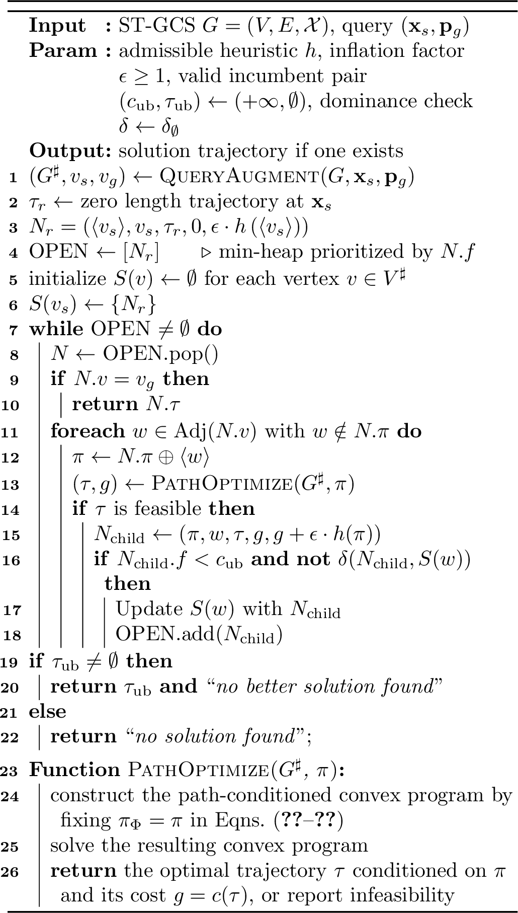
Alg. 5 summarizes the procedure. The solver creates the root node \(N_r\) corresponding to the trivial path \(\langle v_s \rangle\), inserts into OPEN, and stores it in \(S(v_s)\) (Lines [alg:st95search:root95trajectory]–[alg:st95search:def95S]). The map \(S\) defined by \(S(v) = \{N\,|\,N.v=v\}\) records the accepted search nodes that arrive at each vertex \(v\). These stored nodes are used by dominance checks. At each iteration, the solver expands the node \(N\) with the smallest \(f\)-value in OPEN (Lines [alg:st95search:loop95st]–[alg:st95search:pop95OPEN]). If \(N.v = v_g\), the stored trajectory \(N.\tau\) is returned as a solution (Lines [alg:st95search:goal95cond]–[alg:st95search:return95sol]). Otherwise, the solver expands \(N\) by considering each adjacent vertex \(w\) of \(N.v\) that does not already appear in \(N.\pi\) (Lines [alg:st95search:expand95node95start]–[alg:st95search:add95child95to95OPEN]). For each extended path \(\pi = N.\pi \oplus \langle w \rangle\), the solver calls PathOptimize to solve the corresponding path-conditioned convex program. If the program is feasible, a child node is created (Lines [alg:st95search:partial95traj95opt]–[alg:st95search:create95child]). The child node is discarded if its key is no smaller than the input cost upper bound \(c_\text{ub}\), or if the dominance check \(\delta\) certifies that it is dominated by accepted nodes in \(S(w)\). Otherwise, the child node is inserted into both \(S(w)\) and OPEN, and previously accepted nodes in \(S(w)\) that are dominated by the child node are removed (Lines [alg:st95search:create95child]–[alg:st95search:add95child95to95OPEN]). If OPEN becomes empty, the solver returns the incumbent trajectory \(\tau_\text{ub}\) if one was provided; otherwise, it reports failure (Lines [alg:st95search:return95incumbent]–[alg:st95search:fail]).
5.3.1 Upper-Bound Pruning with \(c_\text{ub}\)↩︎
Alg. 5 uses an optional input cost upper bound \(c_\text{ub}\) to avoid exploring nodes that cannot improve the current incumbent, inspired by the spatial GCS search [46]. If no incumbent is available, it uses \(c_\text{ub}= +\infty\) and \(\tau_\text{ub}=\emptyset\). If \(c_\text{ub}< +\infty\), it must be paired with a corresponding feasible incumbent trajectory \(\tau_\text{ub}\) for the same query, with \(c(\tau_\text{ub})=c_\text{ub}\). This ensures that, if all remaining nodes are pruned by the upper-bound test, the solver can still return a valid trajectory.
We obtain \(\tau_\text{ub}\) using a fast vertex-indexed best-first search on the same query-augmented ST-GCS \(G^\sharp\). This auxiliary search still generates graph paths and calls PathOptimize to validate each path and compute its trajectory, but it applies the standard duplicate-pruning rule from graph search. For each arrival vertex, it keeps only the lowest-cost node found so far and discards later nodes arriving at the same vertex with no smaller cost. As discussed in Sec. 5.1, this vertex-indexed pruning is not sound for optimal planning on ST-GCSs, as future costs depend on the entire prefix path. We therefore use this auxiliary search only to obtain a feasible incumbent. If it reaches \(v_g\), the returned trajectory is feasible because it is produced by PathOptimize, and its cost provides a valid \(c_\text{ub}\) for Alg. 5.
5.3.2 Pruning with Dominance Checks \(\delta\)↩︎
We now define the dominance relation used by the optional check \(\delta\) on Line [alg:st95search:dc] of Alg. 5. Since search nodes are path-indexed, dominance is defined through the path-conditioned optimal solution cost \(J^*(\cdot)\) (Definition 2). Consider two search nodes \(N\) and \(N'\) with the same arrival vertex \(v\). We say that \(N'\) dominates \(N\) if \(J^*(N'.\pi)\leq J^*(N.\pi)\). A dominance check \(\delta(N,S(N.v))\) is safe if it returns true only when there exists a retained node \(N'\in S(N.v)\) that dominates \(N\). Safe checks are sufficient but may be conservative. They need not detect all dominated nodes, and they only compare nodes pairwise rather than detecting whether a set of nodes jointly dominate another node. In contrast, heuristic dominance checks may prune without certifying this relation and therefore do not by themselves preserve the theoretical guarantee.
5.3.3 Optimality with Safe Pruning↩︎
The following theorem states the optimality guarantee for Alg. 5 when the pruning operations used on Line [alg:st95search:dc] are safe.
Theorem 1 (\(\epsilon\)-Optimality). For any \(\epsilon\geq 1\), with an admissible heuristic \(h\), a valid incumbent pair \((c_\text{ub},\tau_\text{ub})\), and a safe dominance check, Alg. 5 returns an \(\epsilon\)-optimal trajectory for the query on the input ST-GCS whenever a feasible trajectory exists. In particular, when \(\epsilon=1\), the returned trajectory is cost-optimal.
Let \(c^*\) be the optimal trajectory cost. Because the graph is finite and Lemma 1 lets us restrict attention to simple prefixes, the search space is finite. If \(\tau_\text{ub}\neq\emptyset\) and \(c_\text{ub}\leq \epsilon c^*\), returning \(\tau_\text{ub}\) is already \(\epsilon\)-optimal. Any goal returned before the incumbent has passed the upper-bound test, so its key, and hence its cost, is smaller than \(c_\text{ub}\leq\epsilon c^*\). Thus, it remains to consider the complementary case. Either no incumbent is available or \(c_\text{ub}>\epsilon c^*\). In both cases, upper-bound pruning keeps every node with key at most \(\epsilon c^*\).
We maintain the following invariant: until termination, OPEN contains a representative node \(N\) with \(J^*(N.\pi)=c^*\) and \(N.f\leq \epsilon c^*\). Initially this holds for the root because \(\langle v_s\rangle\) prefixes every feasible trajectory and admissibility gives \(N_r.f=\epsilon h(\langle v_s \rangle)\leq \epsilon c^*\). If OPEN expands a non-representative node, the representative remains in OPEN unless the expanded node is a goal; in that case the minimum-key rule and \(h=0\) imply that the returned trajectory has cost at most \(\epsilon c^*\).
It remains to show that the invariant is preserved when a representative node \(N\) is expanded. If \(N.v=v_g\), then \(N.\tau\) is an optimal solution. Otherwise, take an optimal \(N.\pi\)-consistent solution of cost \(c^*\), and let \(w\) be its next vertex, giving the feasible prefix \(\pi'=N.\pi\oplus\langle w\rangle\). Then PathOptimize creates a child \(M\) with \(M.\pi=\pi'\) and \(J^*(M.\pi)=c^*\). By admissibility, we have \[\begin{align} M.f &=M.g+\epsilon h(M.\pi)\\ &\leq M.g+\epsilon(c^*-M.g) =\epsilon c^*-(\epsilon-1)M.g \leq \epsilon c^*. \end{align}\] By the case assumption above, upper-bound pruning keeps \(M\). If \(M\) is inserted into OPEN, the invariant follows. If \(M\) is pruned by a safe dominance check, some \(M'\in S(w)\) satisfies \(J^*(M'.\pi)\leq J^*(M.\pi)=c^*\). Optimality of \(c^*\) gives \(J^*(M'.\pi)=c^*\), and the same admissibility argument gives \(M'.f\leq\epsilon c^*\). Thus \(M'\) is a valid representative if it is in OPEN; if it has already been expanded, the same argument applied at its expansion transfers the representative to an OPEN descendant or to a retained node safely dominating such a descendant. Likewise, if a retained representative is later removed from \(S(w)\), safety implies that the newly accepted node has \(J^*=c^*\) and key at most \(\epsilon c^*\). Safe dominance pruning therefore transfers, but never eliminates, all representatives before termination.
The incumbent-return case was handled above. In the complementary case, the invariant prevents OPEN from becoming empty before termination, so Alg. 5 must return a goal node \(N_g\) expanded from OPEN. The invariant and the minimum-key rule give \(N_g.f\leq\epsilon c^*\); since \(h(N_g.\pi)=0\), \(c(N_g.\tau)=N_g.g=N_g.f\leq\epsilon c^*\). Setting \(\epsilon=1\) gives cost optimality.
5.4 Pairwise Dominance Checks↩︎
We now present three pairwise dominance checks as the optional check \(\delta\) used in Alg. 5. Throughout this subsection, let \(N\) be a newly generated node and \(N'\in S(N.v)\) be a retained node with the same arrival vertex \(v=N.v=N'.v\). The trivial case is \(v = v_g\), where both nodes already represent solution trajectories, and exact dominance reduces to directly comparing their trajectory costs. The checks below are therefore described for non-goal vertices \(v \neq v_g\). Each check compares \(N\) only with each retained node \(N'\), rather than testing whether several retained nodes jointly dominate \(N\). This pairwise restriction affects pruning power but not correctness when the check is safe.
Recall from Sec. 5.3.2 that \(N'\) dominates \(N\) if \(J^*(N'.\pi)\leq J^*(N.\pi)\). A dominance check is safe if it returns true only when this dominance relation is guaranteed to hold for some \(N'\in S(N.v)\). Among the three checks below, \(\delta_\text{set}\) is safe, while \(\delta_\text{state}\) and \(\delta_\text{pos}\) are heuristic checks that trade optimality guarantees for stronger empirical pruning.
5.4.1 Safe Set-Containment Check \(\delta_\text{set}\)↩︎
The set-containment check \(\delta_\text{set}\) certifies dominance by showing that \(N'\) can reach every state that an \(N.\pi\)-consistent trajectory may reach after entering the shared vertex \(v\). Let \(N.\pi = \langle v_s,\ldots,u,v\rangle\) and define the arrival set \[\begin{align} \label{eqn:R95N} R_N=X_u\cap X_v\cap\{\mathbf{x} \mid \mathbf{x}.t\geq N.\mathbf{x}.t\}. \end{align}\tag{13}\] The set \(R_N\) contains all states that any \(N.\pi\)-consistent solution trajectory may use to enter \(v\). Continuity (Eqn. (4 )) requires membership in the predecessor interface \(X_u\cap X_v\), and \(N.\mathbf{x}.t\) is the earliest arrival time achieved by the path-conditioned optimum for \(N.\pi\). For a space-time state \(\mathbf{x}\), define its forward reachable generalized cone under the velocity limits by \[\begin{align} C(\mathbf{x})=&\{\mathbf{z}\in\mathbb{R}^{m+1}\mid \mathbf{z}.t\geq \mathbf{x}.t,\\ &-\mathbf{v}_{\mathrm{lim}}(\mathbf{z}.t-\mathbf{x}.t) \preceq \mathbf{z}.\mathbf{p}-\mathbf{x}.\mathbf{p} \preceq \mathbf{v}_{\mathrm{lim}}(\mathbf{z}.t-\mathbf{x}.t)\}. \end{align}\] Thus, \(C(\mathbf{x})\) contains all states reachable from \(\mathbf{x}\) by a single time-forward segment satisfying the velocity bounds. Then \(\delta_\text{set}\) is defined by \[\label{eqn:delta95esc} \begin{align} \delta_\text{set}(N,S) \equiv {} & \exists\, N' \in S(N.v), \\ & \boldsymbol{s.t. } \forall\, \mathbf{x} \in R_N,\; C(\mathbf{x}) \subseteq C(N'.\mathbf{x}). \end{align}\tag{14}\] In implementation, since \(R_N\) is convex, it is sufficient to check whether every corner of \(R_N\) lies in \(C(N'.\mathbf{x})\) by transitivity of the cone reachability relation under the same velocity limits.
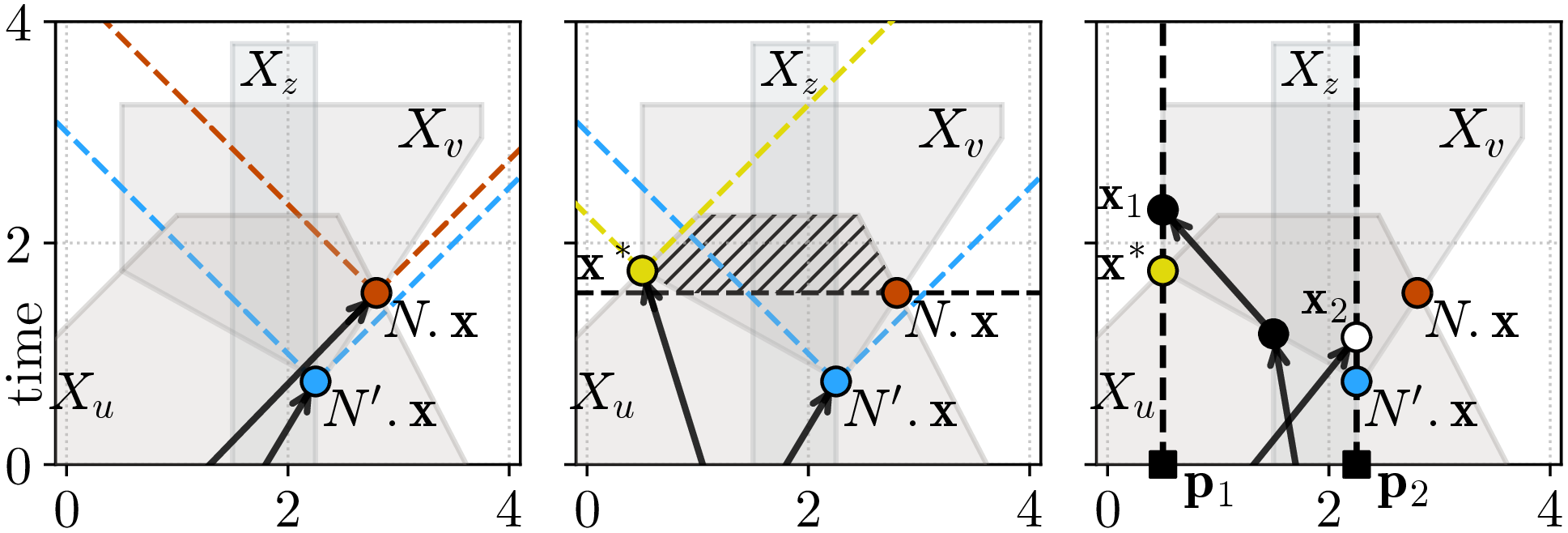
Lemma 2 (Safety of \(\delta_\text{set}\)). If \(\delta_\text{set}(N,S(N.v))\) is true, then \(N\) is dominated by a retained node \(N'\in S(N.v)\).
Let \(N'\in S(N.v)\) satisfy Eqn. (14 ). Consider any \(N.\pi\)-consistent solution trajectory \(\bar{\tau}\). Let \(\mathbf{x}\) and \(\mathbf{y}\) be the states where \(\bar\tau\) enters and exits \(X_{N.v}\), respectively. By construction, \(\mathbf{x}\in R_N\). Moreover, the segment \(\mathbf{x}\rightarrow\mathbf{y}\) is part of \(\bar{\tau}\) within \(X_{N.v}\), so \(\mathbf{y}\in C(\mathbf{x})\). Eqn. (14 ) gives \(C(\mathbf{x})\subseteq C(N'.\mathbf{x})\), and therefore \(\mathbf{y}\in C(N'.\mathbf{x})\). Since \(N'.\mathbf{x}, \mathbf{y} \in X_{N.v}\), the straight segment \(N'.\mathbf{x}\rightarrow\mathbf{y}\) remains in \(X_{N.v}\) and satisfies the time-monotonicity and velocity constraints. Replacing the zero-duration terminal segment of \(N'.\tau\) with this segment, and then concatenating the suffix of \(\bar\tau\) after \(\mathbf{y}\), yields a solution trajectory with the same time cost as \(\bar\tau\). Since this holds for every \(N.\pi\)-consistent solution trajectory, we have \(J^*(N'.\pi)\leq J^*(N.\pi)\). Thus, \(N'\) dominates \(N\).
5.4.2 Heuristic Arrival-State-Containment Check \(\delta_\text{state}\)↩︎
The arrival-state-containment check \(\delta_\text{state}\) approximates \(\delta_\text{set}\) by testing only the stored witness state \(N.\mathbf{x}\), rather than all states in \(R_N\). Then \(\delta_\text{state}\) is defined by \[\begin{align} \delta_\text{state}(N,S) \equiv& \,\exists\, N'\in S(N.v),\\ &\boldsymbol{s.t. } C(N.\mathbf{x})\subseteq C(N'.\mathbf{x}). \end{align}\] This check is cheaper than \(\delta_\text{set}\) because it only compares two cones. It is heuristic since \(N.\mathbf{x}\) is only the stored witness state of the prefix-optimal trajectory for \(N.\pi\), while an optimal \(N.\pi\)-consistent solution trajectory may use a different state to enter \(X_{N.v}\).
5.4.3 Heuristic Position-Based Dominance Check \(\delta_\text{pos}\)↩︎
The set-containment check \(\delta_\text{set}\) can be expensive because it reasons over all states in \(R_N\). A cheaper alternative is to compare two prefixes only at a sampled spatial position \(\mathbf{p}\in\{\mathbf{x}.\mathbf{p}\,|\,\mathbf{x}\in X_{N.v}\}\). For a generated search node \(N\), let \(J_\mathbf{p}(N.\pi)\) denote the cost of the optimal trajectory conditioned on \(N.\pi\) whose terminal state in \(X_v\) has spatial position \(\mathbf{p}\), with \(J_\mathbf{p}(\pi) = +\infty\) if no such trajectory exists. Then \(\delta_\text{pos}\) is defined by \[\begin{align} \delta_\text{pos}(N,S) \equiv &\,\exists\,N'\in S(N.v),\\ &\boldsymbol{ s.t. } J_\mathbf{p}(N'.\pi)\leq J_\mathbf{p}(N.\pi). \end{align}\] This check can be strengthened by using multiple sampled positions. In the limiting case of covering all relevant positions in \(X_{N.v}\), it can certify a safe pairwise dominance relation between \(N\) and a retained node \(N'\). One can further extend the idea to certify joint dominance by allowing different retained nodes in \(S(N.v)\) to dominate \(N\) at different positions. These extensions are more expensive. Experimentally, we use only one sampled position, so \(\delta_\text{pos}\) remains heuristic.
5.4.4 Comparison and Use with Upper-Bound Pruning↩︎
Fig. 6 illustrates the difference between the three pairwise dominance checks. The \(\delta = \delta_\text{set}\) check reasons over all relevant states in \(R_N\), \(\delta_\text{state}\) only compares the stored witness states, and \(\delta_\text{pos}\) compares the prefixes at sampled spatial positions. In our implementation, upper-bound pruning is applied before one of these dominance checks. When the input \(\delta = \delta_\emptyset\) or \(\delta = \delta_\text{set}\), the guarantee in Theorem 1 applies. When \(\delta_\text{state}\) or \(\delta_\text{pos}\) is used, the solver becomes heuristic and can run substantially faster, but the pruning no longer preserves the optimality guarantee. Combining upper-bound pruning with heuristic dominance checks is empirically effective but can make the search more likely to return the incumbent trajectory. The heuristic checks may remove nodes that would otherwise lead to a feasible solution, while the upper-bound test further restricts the search to trajectories with cost strictly below \(c_\text{ub}\). Thus, a solution that the heuristic search might find without upper-bound pruning can be discarded if it is no better than the incumbent. In that case, Alg. 5 falls back to the stored incumbent trajectory \(\tau_\text{ub}\). Among the two heuristic checks, \(\delta_\text{pos}\) is usually more aggressive because it compares prefixes only through sampled spatial positions and may miss useful unsampled states. The check \(\delta_\text{state}\) is also heuristic, but remains tied to the actual stored witness states through cone containment. This makes \(\delta_\text{pos}\) generally more sensitive to upper-bound pruning, while \(\delta_\text{state}\) tends to be more conservative in practice.
5.5 Admissible Heuristics↩︎
We now describe admissible heuristics for Alg. 5. All heuristics below are defined to be zero when \(N.v = v_g\), since \(N.\tau\) is already a solution trajectory. Thus, the definitions in this subsection focus on non-goal nodes \(N.v \neq v_g\). By Definition 3, an admissible heuristic must lower-bound the optimal remaining solution cost from a prefix path \(N.\pi\), rather than the cost-to-go from the stored witness state \(N.\mathbf{x}\) alone. This distinction is important because \(N.\mathbf{x}\) is only the stored witness state of the trajectory optimized for \(N.\pi\); after extending the path, the optimal trajectory may pass through a different state in \(X_{N.v}\). Thus, a heuristic evaluated from \(N.\mathbf{x}\) can overestimate the optimal remaining solution cost for the path-indexed node, as illustrated in Fig. 7.

For a non-goal node \(N\), we define the prefix interface \[\label{eqn:prefix95interface} I_N = \begin{cases} \{\mathbf{x}_s\}, & \text{if } N.\pi=\langle v_s\rangle,\\ X_u\cap X_v, & \text{if } N.\pi=\langle v_s,\ldots,u,v\rangle, \end{cases}\tag{15}\] which is a useful source set for computing heuristics, as any \(N.\pi\)-consistent trajectory must pass through some state in \(I_N\) before continuing beyond the prefix.
A general way to construct admissible heuristics is to relax different subsets of constraints in the path-conditioned ST-GCS problem. The original problem enforces graph topology, set membership, continuity between adjacent sets, motion constraints, and the query-specific goal-position constraint. The three heuristics below represent different choices. The \(h_\text{mot}\) heuristic keeps only the motion constraints, \(h_\text{tri}\) keeps local set-membership and motion constraints but relaxes continuity across local transitions, and \(h_\text{tab}\) uses precomputed true interface-to-set costs with an online correction to the query goal position.
Offline precomputation can use the static environment and any dynamic obstacles known before the query. Query-specific information, such as \(\mathbf{x}_s\), \(\mathbf{p}_g\), and \(v_g\), is incorporated online after query augmentation. In MRMP, trajectories of previously planned robots are not known during offline preprocessing; the resulting ECD-updated ST-GCSs only remove feasible space, so lower bounds computed on the initial ST-GCS remain admissible relaxations, as discussed later in Sec. 7.
For the ST-GCS trajectory representation in Sec. 4.1, we define the following useful quantity for query-specific online computation. For a set \(Y\) of space-time states, define the velocity-only travel-time lower bound to the query goal position by \[\begin{align} \rho(Y, \mathbf{p}_g)=\min_{\mathbf{x}\in Y}\left\|(\mathbf{p}_g-\mathbf{x}.\mathbf{p})\oslash\mathbf{v}_{\mathrm{lim}}\right\|_\infty \end{align}\] with value of \(+\infty\) if \(Y=\emptyset\), where \(\oslash\) denotes element-wise division. Since the query specifies a goal position with free arrival time, all our heuristics estimate the cost to \(\mathbf{p}_g\) rather than to a fixed goal state.
5.5.1 Motion-Only Heuristic \(h_{\mathrm{mot}}\)↩︎
This heuristic relaxes all the graph-topology and set-membership constraints after the prefix and keeps only the motion constraints needed to reach goal \(\mathbf{p}_g\). In a more general setting, \(h_{\mathrm{mot}}\) is the minimum travel cost from some state in \(I_N\) to any state with spatial position \(\mathbf{p}_g\), subject only to the chosen motion constraints. For our ST-GCS trajectory representation, the retained motion constraints are time monotonicity and component-wise velocity limits. Therefore, \(h_{\mathrm{mot}}\) is defined by \[\begin{align} h_{\mathrm{mot}}(N.\pi)= \rho(I_N, \mathbf{p}_g). \end{align}\] This is a lightweight online heuristic. Compared with estimating from any state in \(X_{N.v}\) [45], using \(I_N\) is stronger because it respects the predecessor–current-set interface induced by the prefix path.
Lemma 3. The heuristic \(h_\text{mot}\) is admissible.
Consider any \(N.\pi\)-consistent trajectory \(\bar\tau\). Let \(\mathbf{x} \in I_N\) be the state through which \(\bar\tau\) passes before continuing beyond the prefix. The prefix portion of \(\bar\tau\) has cost at least \(N.g\) as \(N.g\) is the optimal cost conditioned on \(N.\pi\). The remaining portion from \(\mathbf{x}\) to \(\mathbf{p}_g\) satisfies the the velocity limits, so its cost is at least \(\rho(\{\mathbf{x}\}, \mathbf{p}_g)\), and therefore at least \(\rho(I_N, \mathbf{p}_g)\). Thus, \(c(\bar\tau) \geq N.g + h_\text{mot}\) holds for any \(N.\pi\)-consistent solution trajectory \(\bar\tau\).
5.5.2 Triplet-Relaxation Heuristic \(h_{\mathrm{tri}}\)↩︎
This heuristic keeps the graph topology and local constraints within each convex set, but relaxes continuity between consecutive local transitions. A similar idea has been used by spatial GCS solvers [46], [55]. For each input-graph triplet \((u,v,w)\) with \(u,v,w\in V\) and \(u,w\) adjacent to \(v\) in \(G\), a local lower-bound cost is precomputed for moving through \(X_v\) from the interface \(X_u\cap X_v\) to the interface \(X_v\cap X_w\), subject to the same local set-membership and motion constraints. In our piecewise-linear instantiation, this cost is computed offline by a local convex program over one segment inside \(X_v\) with time monotonicity and velocity limits, denoted by \(q(u,v,w)\). If no such segment exists, \(q(u,v,w) = +\infty\). At query time, costs of query-specific triplets induced by the auxiliary goal vertex \(v_g\) of the form \(q(u,v,v_g)\) are computed online by a local convex program similarly. For \(N.\pi=\langle\ldots,u,v\rangle\), let \(\Pi^\text{suf}_N\) denote the set of all the suffixes with its predecessor \(u\), where each \(\pi\in \Pi^\text{suf}_N\) is in the form of \(\pi=\langle u, v=w_0,\ldots,w_l = v_g \rangle\) ending at \(v_g\). We define \(h_{\mathrm{tri}}\) as the minimum accumulated relaxed triplet cost over \(\Pi^\text{suf}_N\) by \[\begin{align} h_{\mathrm{tri}}(N.\pi) = &\min_{\pi\in \Pi^\text{suf}_N}\Big[q(u, w_0, w_1)+ \sum_{i=1}^{l-1} q(w_{i-1},w_{i},w_{i+1})\Big], \end{align}\] where the first term is omitted if \(u = v_s\), and the summation is omitted if \(l=1\). For the root node \(N.\pi = \langle v_s \rangle\), it omits the first two triplets and minimizes over the first input-graph vertex \(w_1\) after \(v_s\). The minimization is computed online as a shortest-path problem on the induced triplet graph, e.g., by Dijkstra’s algorithm [63].
Lemma 4. The heuristic \(h_{\text{tri}}\) is admissible.
Fix any \(N.\pi\)-consistent trajectory. Its suffix induces a sequence of triplets. For each triplet, the actual segment through the middle convex set is feasible for the corresponding triplet subproblem, so the triplet cost is at most the actual segment cost. Omitting query-specific start triplets only further relaxes the cost. Summing these inequalities over the suffix lower bounds the optimal remaining solution cost. Since \(h_{\text{tri}}\) takes the minimum over all suffixes in the relaxed triplet graph, it is at most the remaining cost of any \(N.\pi\)-consistent trajectory beyond the prefix represented by \(N.\pi\).
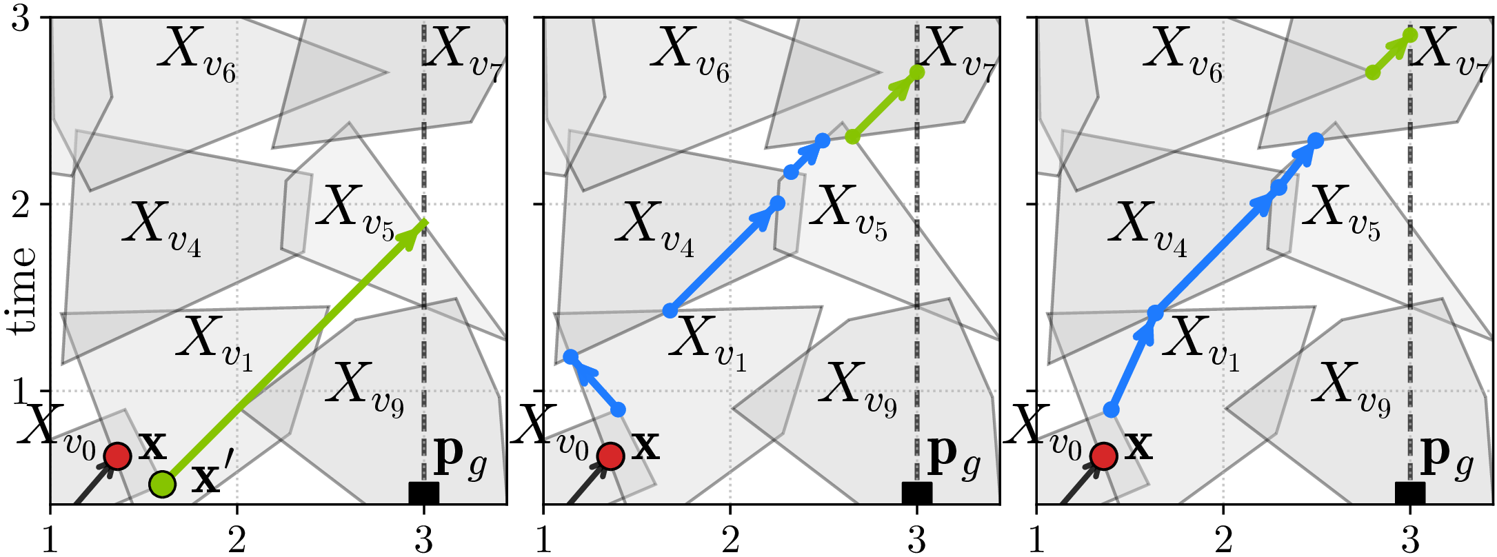
5.5.3 Interface-to-Set Cost Table Heuristic \(h_\text{tab}\)↩︎
This heuristic precomputes stronger lower bounds by solving interface-to-set problems offline and storing their solution costs in a table. For any input-graph interface \(I=X_u\cap X_v\) with \(u, v \in V\) and any input-graph vertex \(w\in V\), let \(d(I,w)\) denote the minimum trajectory cost of reaching any state in \(X_w\) from any state in \(I\), over all graph paths, subject to the same graph, set-membership, continuity, and motion constraints. These values can be precomputed offline for all interfaces and all vertices by running Alg. 5 to solve the corresponding interface-to-set problems. They are query independent because they start from input-graph interfaces and end at input-graph sets. For a non-goal search node \(N\), define the relaxed table-start value by \[\begin{align} &\hat{d}_N(v_p) = \\ &\quad\begin{dcases} \min_{v\in\operatorname{Adj}(v_s)\cap V \atop w\in\operatorname{Adj}(v)\cap V} d(X_v\cap X_w, v_p), & \text{if } N.v = v_s,\\ \min_{w\in\operatorname{Adj}(N.v)\cap V} d(X_{N.v}\cap X_w, v_p), & \text{if } N.\pi = \langle v_s, N.v\rangle,\\ d(I_N, v_p), & \text{otherwise}. \end{dcases} \end{align}\] The first two cases handle query-specific start interfaces by omitting the nonnegative cost from \(\mathbf{x}_s\) to the first input-graph interface used by the cost table. For a non-goal \(N\) with \(N.v\notin\operatorname{Adj}(v_g)\), we define the heuristic by \[h_{\mathrm{tab}}(N.\pi)= \min_{\substack{ v_p\in \operatorname{Adj}(v_g)\cap V\\ u\in\operatorname{Adj}(v_p)\cap V}} \left[ \hat{d}_N(v_p)+\rho(X_u\cap X_{v_p}, \mathbf{p}_g) \right].\] If \(N.v \in \operatorname{Adj}(v_g)\), we instead set \(h_{\mathrm{tab}}(N.\pi)=\rho(I_N,\mathbf{p}_g)\).
Lemma 5. The heuristic \(h_\text{tab}\) is admissible.
If \(N.v \in \operatorname{Adj}(v_g)\), then \(h_{\mathrm{tab}}(N.\pi) = \rho(I_N, \mathbf{p}_g)\) is admissible by the same argument as Lemma 3. Now consider \(N.v \notin \operatorname{Adj}(v_g)\bigcup \{v_g\}\) and any \(N.\pi\)-consistent solution trajectory \(\bar\tau\). Let \(v_p\in \operatorname{Adj}(v_g)\cap V\) be the input-graph vertex through which the vertex path of \(\bar\tau\) reaches \(v_g\), and let \(u\in\operatorname{Adj}(v_p)\cap V\) be the input-graph vertex preceding \(v_p\) on that path. If \(I_N\) is an input-graph interface, the portion from \(I_N\) to \(X_{v_p}\) has cost at least \(d(I_N,v_p)\). If \(I_N\) is query-specific because \(N.v = v_s\) or \(N.\pi = \langle v_s, N.v\rangle\), then \(\hat{d}_N(v_p)\) starts from a later input-graph interface and omits only nonnegative cost needed to reach that interface, so it remains a lower bound. The final portion from \(X_u\cap X_{v_p}\) to \(\mathbf{p}_g\) satisfies the velocity limits and is lower-bounded by \(\rho(X_u\cap X_{v_p},\mathbf{p}_g)\). Thus, the corresponding term in the minimization defining \(h_\text{tab}\) is no larger than the remaining cost of \(\bar\tau\). Since \(h_\text{tab}\) minimizes over all such pairs \((u,v_p)\), it is also no larger than the remaining cost of \(\bar\tau\), for any \(N.\pi\)-consistent solution trajectory.
5.5.4 Comparison and Maximum Heuristic \(h_\text{max}\)↩︎
Fig. 8 illustrates the three heuristics above on an example query. They capture complementary relaxations of the optimal remaining solution cost from a prefix path. The maximum heuristic \(h_\text{max}\) combines them by taking their pointwise maximum: \[\begin{align} h_{\text{\normalfont max}}(N.\pi) = \max\left\{ h_\text{mot}(N.\pi), h_\text{tri}(N.\pi), h_\text{tab}(N.\pi) \right\}. \end{align}\] This preserves the strongest available lower bound at each search node.
Lemma 6. The heuristic \(h_\text{max}\) is admissible.
Each component heuristic is no larger than the optimal remaining solution cost from \(N.\pi\) by Lemmas 3, 4, and 5. The maximum of several lower bounds is still a lower bound, so \(h_\text{max}\) is admissible.
6 Trajectory Occupancy Reservation↩︎
This section presents the Exact Convex Decomposition (ECD) scheme for reserving piecewise-linear trajectory occupancies in an ST-GCS. Given the spatiotemporal occupancy of a moving object, such as a robot or a dynamic obstacle, ECD removes the occupied region from the relevant space-time convex sets and decomposes the remaining free space into convex subsets. The resulting ST-GCS can then be used for subsequent planning queries that must avoid the reserved trajectory in space-time.
6.1 Spatiotemporal Trajectory Occupancy↩︎
We assume that each moving object, including a robot or a dynamic obstacle, is represented by a piecewise-linear center trajectory \(\tau=\langle\mathbf{x}_1,\ldots,\mathbf{x}_l\rangle\) in \((m+1)\)-dimensional space-time with radius \(r > 0\). At each time, the object is centered at the position \(\mathbf{x}.\mathbf{p}\) of state \(\mathbf{x}\) along \(\tau\) and occupies a spatial collision body of hypercube \[\begin{align} \label{eqn:hypercube95occ} \boxdot (\mathbf{x}.\mathbf{p}, r)=\{\mathbf{p} \mid ||\mathbf{p}-\mathbf{x}.\mathbf{p}||_\infty \leq r\}\subseteq \mathbb{R}^{m}. \end{align}\tag{16}\] Let \(\Psi(\mathbf{x}_i,\mathbf{x}_{i+1},r)\) be the parallelotope obtained by sweeping the spatial \(\boxdot (\mathbf{x}.\mathbf{p}, r)\) along each segment \(\mathbf{x}_i\rightarrow \mathbf{x}_{i+1}\) of \(\tau\). A piecewise-convex spatiotemporal occupancy for trajectory \(\tau\) with object radius \(r\) can be defined by \[\begin{align} \label{eqn:traj95occ} \Omega(\tau, r)=\bigcup_{i=1}^{l-1} \Psi (\mathbf{x}_i,\mathbf{x}_{i+1},r)\subseteq \mathbb{R}^{m+1}. \end{align}\tag{17}\]
Consider a robot with radius \(r\) and another moving object with trajectory \(\tau\) and radius \(r'\). An ST-GCS without any intersections with \(\Omega(\tau, r+r')\) naturally represents the collection of the space-time collision-free space for the robot. In the next section, we introduce the ECD scheme, which aims to reserve (i.e., remove) any occupancy represented as in Eqn. (17 ) from an ST-GCS. Fig. 10 illustrates two piecewise-linear trajectories and their reserved occupancies in 1D and 2D spaces.
6.2 Exact Convex Decomposition (ECD)↩︎
ECD reserves trajectory occupancy on an arbitrary ST-GCS \(G=(V,E,\mathcal{X})\) using a piecewise-linear trajectory \(\tau=\langle\mathbf{x}_{1},\ldots,\mathbf{x}_{l}\rangle\) and a safe clearance parameter \(R\) as input. As aforementioned, \(R\) is typically the sum of the radii of two objects, with a positive offset if needed. For each parallelotope piece \(\Psi (\mathbf{x}_i,\mathbf{x}_{i+1},R)\in\Omega(\tau, R)\) of \(\tau\), it may intersects multiple convex sets of \(G\). On the other hand, a convex set of \(G\) might also contain multiple parallelotope occupancy pieces. To account for above cases, ECD subdivides \(\tau\) and constructs an ordered sequence of vertex–segments tuples \(L_v=\langle(\mathbf{x}_j,\mathbf{y}_j)\rangle_{j=1}^{\eta_v}\) for each \(v\in V\), such that for every \(j=1,\ldots,\eta_v\), it satisfies that \(\Psi (\mathbf{x}_j,\mathbf{y}_j,R)\cap X_v\neq\emptyset\) and that \(\mathbf{y}_{j}.t\leq \mathbf{x}_{j+1}.t\) if \(j\neq \eta_v\). Intuitively speaking, each sequence \(L_v\) collects the time-sorted subdivided segments of \(\tau\) whose occupancies intersect with \(X_v\in\mathcal{X}\). Writing \(\mathcal{L}\) for all collected vertex–segment tuples, we have \[\begin{align} \bigcup_{(v, \mathbf{x},\mathbf{y})\in \mathcal{L}} \Psi (\mathbf{x},\mathbf{y},R)=\Omega(\tau, R) \end{align}\]
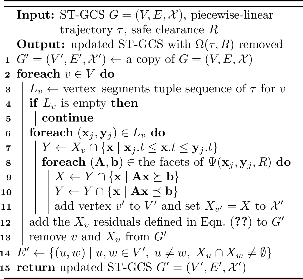

Alg. 9 summarizes the ECD scheme. It starts by iterating each vertex \(v\in V\) and collects the corresponding vertex–segments tuple sequence \(L_v\) from \(\tau\) (Lines [alg:ecd:iterate95V]-[alg:ecd:build95occ]). If \(L_v\) is not empty, ECD replaces \(X_v\) by a convex decomposition of \(X_v\setminus\Omega(\tau, R)\) (Lines [alg:ecd:iterate95occ]–[alg:ecd:add95residuals]) and removes the original \(v\) and \(X_v\) from \(G'\) (Line [alg:ecd:remove]). For each segment \(\mathbf{x}_j\rightarrow\mathbf{y}_j\) from \(L_v\), it slices only the time-bounded subset \(Y\subseteq X_v\) (Line [alg:ecd:time95restricted95Y]). Using each facet of the parallelotope occupancy \(\Psi(\mathbf{x}_j,\mathbf{y}_j,R)\) as the separating hyperplane (Line [alg:ecd:iterate95facet]), ECD creates outside convex pieces disjoint from the parallelotope (Line [alg:ecd:slice95side]) and updates the residual on the occupancy side (Line [alg:ecd:exclude95outside]). By convention, each facet \((\mathbf{A},\mathbf{b})\) is formed such that the convex set \(\{\mathbf{x}\mid\mathbf{A}\mathbf{x}\preceq \mathbf{b}\}\) contains parallelotope \(\Psi(\mathbf{x}_j,\mathbf{y}_j, R)\). After the subdivision by each time-bounded \(Y\), there remain three types of \(X_v\) residuals that are outside the interiors of the time-bounded subsets \(Y\) and thus need to be added back to \(G'\) if nonempty (Line [alg:ecd:add95residuals]). We define the three types of \(X_v\) residuals as follows: \[\label{eqn:residuals95Xv} \begin{align} &X_v\cap\{\mathbf{x}\mid \mathbf{x}.t\leq\mathbf{x}_1.t\},\\ &X_v\cap\{\mathbf{x}\mid \mathbf{y}_{j-1}.t\leq\mathbf{x}.t\leq\mathbf{x}_{j}.t\}, &&\forall j=2,\ldots,\eta_v,\\ &X_v\cap\{\mathbf{x}\mid \mathbf{x}.t\geq\mathbf{y}_{\eta_v}.t\} \end{align}\tag{18}\]
Finally, ECD rebuilds the adjacency of \(G'\) by checking set intersections (Line [alg:ecd:update95edges]), and returns the updated ST-GCS \(G'\) (Line [alg:ecd:return]). The ECD scheme is quite general and applies to various other motions that can be represented by a piecewise-linear space-time trajectory. For example, waiting or in-place turning can be encoded as a segment \((\mathbf{p},t)\to (\mathbf{p},t')\) along \(\tau\) and being reserved in the input ST-GCS. More importantly, as we will see in Sec. 7, pre-start and post-arrival waiting segments should be inserted into the beginning and end of every single-robot trajectory \(\tau\), respectively. As a result, when planning on the ST-GCS with \(\tau\) reserved by ECD, the other robots must avoid the robot that stays at the start and goal positions before and after executing \(\tau\).
7 Multi-Robot Motion Planning↩︎
This section integrates spatiotemporal planning on ST-GCSs and ECD reservation for Multi-Robot Motion Planning (MRMP). The low-level solver solves single-robot queries one at a time with the BFS solver in Sec. 5, while the high-level coordinator resolves inter-robot conflicts by deciding which robot trajectories are reserved in each low-level call.
7.1 Problem Definition↩︎
We consider \(n\) robots with the same radius \(r\) sharing a given base ST-GCS \(G_0=(V_0,E_0,\mathcal{X}_0)\), which represents the collision-free space-time region before inter-robot reservations and may be constructed, for example, by extruding a spatial GCS through time and then applying the ECD scheme to remove occupancies of known dynamic obstacles. Each robot \(i=1,2,\ldots,n\) has a query \((\mathbf{x}_{s,i},\mathbf{p}_{g,i})\) with \(\mathbf{x}_{s,i}=(\mathbf{p}_{s,i},t_{s,i})\in\mathbb{R}^{m+1}\), where the arrival time at \(\mathbf{p}_{g,i}\) is unconstrained.
A feasible solution of any query \((\mathbf{x}_{s,i},\mathbf{p}_{g,i})\) on ST-GCS is a piecewise-linear trajectory \(\tau_i=\langle\mathbf{x}_1,\ldots,\mathbf{x}_l\rangle\), where \(\mathbf{x}_1=\mathbf{x}_{s,i}\) and \(\mathbf{x}_l.\mathbf{p}=\mathbf{p}_{g,i}\). When \(t_{s,i}\neq 0\) or \(\mathbf{x}_{l}.t\neq t_{\max}\), the pre-start or post-arrival staying motions are absent in \(\tau_i\). Planning on an ECD-reserved ST-GCS with such \(\tau_i\) could lead to collisions on \(\mathbf{p}_{s,i}\) during \(t\in[0,t_{s,i}]\) or on \(\mathbf{p}_{g,i}\) during \(t\in[\mathbf{x}_{l}.t,t_{\max}]\). Therefore, we let \(\tilde{\tau}_i\) denote its endpoint-augmented variant, defined as follows: \[\begin{align} \tilde{\tau}_i=\Big\langle(\mathbf{x}_1.\mathbf{p},0),\mathbf{x}_1,\ldots,\mathbf{x}_l,(\mathbf{x}_l.\mathbf{p},t_{\max})\Big\rangle, \end{align}\] A trajectory set \(\mathcal{T}=\{\tau_i\}_{i=1}^n\) is feasible if and only if each \(\tau_i\) is a feasible single-robot trajectory for query \((\mathbf{x}_{s,i},\mathbf{p}_{g,i})\) on \(G_0\), and every robot pair is collision-free under the robot occupancy model defined in Eqn. (17 ): \[\begin{align} \Omega(\tilde{\tau}_j, r)\cap \Omega(\tilde{\tau}_i, r)=\emptyset,\quad \forall\, i\neq j. \end{align}\]
The MRMP problem seeks to find such a feasible trajectory set described above. We evaluate the MRMP solution quality by two common aggregate metrics, namely the sum-of-costs (SOC) and the makespan: \[\begin{align} \mathrm{SOC}(\mathcal{T})=\sum_{i=1}^n c(\tau_i),\, \mathrm{Makespan}(\mathcal{T})=\max_{i=1,\ldots, n} c(\tau_i), \end{align}\] where makespan is the maximum individual trajectory duration, excluding the pre-start waiting time.
For notation, let \(\operatorname{ECD}(G,\tau,R)\) denote the ST-GCS returned by Alg. 9. For an ordered list of trajectories, \(\operatorname{ECD}(G,\langle \tau_1,\ldots,\tau_l\rangle,2r)\) denotes the ST-GCS obtained by applying Alg. 9 successively to \(\tau_1,\ldots,\tau_l\) in that order, with \(\operatorname{ECD}(G,\langle\rangle,2r)=G\). It is worth noting that, for MRMP where the robots have different radii, we only need to construct an individual base \(G_0\) for each robot and change the ECD clearance parameter accordingly, while the low-level single-robot solver and the following high-level coordination algorithms remain unchanged.
7.2 Prioritized Planning with ST-GCS and ECD↩︎
We instantiate Prioritized Planning (PP) [8] in the ST-GCS setting using the BFS solver in Alg. 5 for low-level single-robot planning and ECD for trajectory reservation. We consider a total priority order \(\pmb{\sigma}=\langle \sigma_1, \dots, \sigma_n\rangle\), where \(\pmb{\sigma}\) is a permutation of the robot indices \(1,2,\ldots,n\). Robot \(\sigma_i\) has higher priority than robot \(\sigma_j\) if \(i<j\). PP plans robots sequentially on progressively updated ST-GCSs. When planning for robot \(\sigma_k\), the trajectories of robots \(\sigma_1, \sigma_2,\dots, \sigma_{k-1}\) have already been planned and reserved. Set \(G^{(1)}=G_0\). At iteration \(k\), robot \(\sigma_k\) is planned on \(G^{(k)}\). The low-level solver solves the query \((\mathbf{x}_{s,\sigma_k},\mathbf{p}_{g,\sigma_k})\) on \(G^{(k)}\), so the returned trajectory avoids all higher-priority trajectories, including their endpoint-staying portions. If this call fails, PP reports failure for the priority order \(\pmb{\sigma}\). Otherwise, after obtaining \(\tau_{\sigma_k}\), PP updates the graph for the next iteration by \[\begin{align} \label{eqn:def95Gk} G^{(k+1)}=\operatorname{ECD}(G^{(k)},\tilde{\tau}_{\sigma_k},2r). \end{align}\tag{19}\] After all robots have been processed, PP returns the solution set of trajectories.
We consider the base ST-GCS \(G_0\) constructed by extruding a spatial GCS along the time dimension from \(0\) to \(t_\text{max}\). Without loss of generality, we assume no dynamic obstacles are present to analyze the MRMP solvability on ST-GCS. Let \(t_0 = \max_{i=1,\ldots,n}t_{s,i}\) defines the time when all robots are ready to move. In case there are dynamic obstacles, we shift \(t_0\) to the time when all dynamic obstacles have reached their terminal positions and all robots are ready to go, and the rest analysis remains identical. Let \(\tau_\text{stay}(\mathbf{p},t)=\langle(\mathbf{p},t),(\mathbf{p},t_\text{max})\rangle\) denote the trajectory segment staying at position \(\mathbf{p}\) from some time \(t\leq t_\text{max}\) to \(t_\text{max}\). We further define a sequence \[\begin{align} \mathcal{S}_{i}(t)=\langle &\tau_\text{stay}(\mathbf{p}_{s,j_{1}},t), \ldots, \tau_\text{stay}(\mathbf{p}_{s,j_{n-1}},t),\\ &\tau_\text{stay}(\mathbf{p}_{g,j_1},t), \ldots,\tau_\text{stay}(\mathbf{p}_{g,j_{n-1}},t) \rangle \end{align}\] collecting the start and goal staying trajectories for all robots \(j=j_1,\ldots,j_{n-1}\) and \(j\neq i\). We now define well-formedness conditions for MRMP instances that are sufficient for the completeness of PP on ST-GCS.
Definition 4 (Well-Formedness). The MRMP instance is well-formed if it satisfies the following conditions:
(i) The query starts and goals are pairwise separated, that is, for every pair \(i\neq j\), \(||\mathbf{p}_{s,i}-\mathbf{p}_{s,j}||_\infty\geq 2r\), \(||\mathbf{p}_{g,i}-\mathbf{p}_{g,j}||_\infty\geq 2r\), and \(||\mathbf{p}_{s,i}-\mathbf{p}_{g,j}||_\infty\geq 2r\);
(ii) The robots are also assumed to be able to safely stay at their query start and goal positions indefinitely throughout the time horizon, that is, \[\begin{align} \{\mathbf{x}\mid \mathbf{x}.\mathbf{p}\in\{\mathbf{p}_{s,i}, \mathbf{p}_{g,i}\}, \mathbf{x}.t\in[0,t_\text{max}]\}&\subseteq \bigcup_{v\in V_0} X_v; \end{align}\]
(iii) For each robot \(i=1,\ldots, n\), query \(((\mathbf{p}_{s,i}, t_0),\mathbf{p}_{g,i})\) is feasible on \(\operatorname{ECD}(G_0,\mathcal{S}_{i}(t_0),2r)\) and has an optimal trajectory cost of \(C^*_i\);
(iv) The ST-GCS global time limit \(t_\text{max}\geq t_0+nC\), where \(C=\max\{\epsilon C^*_1,\ldots, \epsilon C^*_n\}\) with \(\epsilon\geq 1\).
Theorem 2 (Completeness of PP). For a well-formed MRMP instance, PP with an \(\epsilon\)-bounded-suboptimal low-level BFS solver returns a feasible trajectory set using an arbitrary total priority order.
Fix any total priority order \(\pmb{\sigma}=\langle \sigma_1,\ldots,\sigma_n\rangle\). Let \(t_k=t_0+(k-1) C\). We prove by induction that, before robot \(\sigma_k\) is planned, every higher-priority robot has reached its goal by time \(t_k\). The claim is trivial for \(k=1\). Assume it holds for \(k\). By induction, all higher-priority robots have reached their goals by time \(t_k\), and they can safely stay at their corresponding goal positions onward by conditions ([wellform:separation]-[wellform:staying]). According to condition ([wellform:feasibility]), we know that query \(((\mathbf{p}_{s,\sigma_k},t_0),\mathbf{p}_{g,\sigma_k})\) is feasible on \(\operatorname{ECD}(G_0,\mathcal{S}_{\sigma_k}(t_0),2r)\) with optimal cost \(C^*_{\sigma_k}\). In fact, \(\mathcal{S}_{\sigma_k}(t_k)\) is a time-padded copy of \(\mathcal{S}_{\sigma_k}(t_0)\) in the sense that each spatial position in \(\mathcal{S}_{\sigma_k}(t_k)\) has the same time offset \(\Delta t = t_k - t_0\geq 0\) compared to each corresponding spatial position in \(\mathcal{S}_{\sigma_k}(t_0)\). Therefore, it is easy to see that a feasible trajectory for query \(((\mathbf{p}_{s,\sigma_k},t_k),\mathbf{p}_{g,\sigma_k})\) with at most \(\epsilon C^*_{\sigma_k}\) cost can always be found by shifting \(\Delta t\) in each state time along an \(\epsilon\)-optimal trajectory for query \(((\mathbf{p}_{s,\sigma_k},t_0), \mathbf{p}_{g,\sigma_k})\), since we know that \[\begin{align} t_k + \epsilon C^*_{\sigma_k} \leq t_0+(n-1)C + \epsilon C^*_{\sigma_k} \leq t_\text{max} \end{align}\] by condition ([wellform:t95max]). Thus, robot \(\sigma_k\) starts at \(t_k\), reaches its goal no later than \(t_{k+1}=t_k+C\geq t_k +\epsilon C^*_{\sigma_k}\), and stays at its goal after arrival while being collision-free with \(\sigma_{k+1},\ldots,\sigma_{n}\) staying at their starts and \(\sigma_1,\ldots,\sigma_{k-1}\) staying at their goals. This proves the induction.
It remains to show that an \(\epsilon\)-bounded-suboptimal low-level solver in PP is certified to plan a trajectory with a cost of at most \(C\) for robot \(\sigma_k\) on \(G^{(k)}\) defined in Eqn. (19 ). Notice that as \(\sigma_k\) departs at time \(t_k\), its feasible solution space regarding each convex set \(X_v\) from \(G^{(k)}\) is a time-bounded subset \(\bar{X}_v=X_v\cap\{\mathbf{x}\mid \mathbf{x}.t\geq t_k\}\). Denote the ST-GCS built from each such \(\bar{X}_v\) as \(\bar{G}^{(k)}\). It is easy to see that the union of all convex sets in \(\operatorname{ECD}(G_0,\mathcal{S}_{\sigma_k}(t_k),2r)\) is a subset of the union in \(\bar{G}^{(k)}\), and then subsequently a subset of the union in \(G^{(k)}\). Therefore, the query \(((\mathbf{p}_{s,\sigma_k},t_k),\mathbf{p}_{g,\sigma_k})\) is always feasible on the larger solution space of \(G^{(k)}\), since we have seen from above that same query is feasible on \(\operatorname{ECD}(G_0,\mathcal{S}_{\sigma_k}(t_k),2r)\). Thus, the \(\epsilon\)-bounded-suboptimal low-level solver finds a trajectory for robot \(\sigma_k\) with at most \(\epsilon C^*_{\sigma_k}\leq C\) cost, which concludes the proof.
7.3 PBS with ST-GCS and ECD↩︎
We instantiate Priority-Based Search (PBS) [22] in the ST-GCS setting by using the BFS solver in Alg. 5 for low-level single-robot planning and ECD for reserving spatiotemporal occupancies. PBS searches over partial priority orders instead of committing to one total priority order. A PBS node \(N\) stores a set \(\boldsymbol{\pmb\prec}_N\) of ordered robot pairs and a trajectory set \(N.\mathcal{T}\). Let \({\prec}_N^+\) denotes the transitive closure of \({\pmb\prec}_N\) such that if \(i\prec^+_N j\), then robot \(j\) must avoid robot \(i\). Namely, its trajectory \(N.\tau_j\) can be obtained by planning on \[\begin{align} \label{eqn:reserve95high95priority} G^{(j)}_N=\operatorname{ECD}(G_0,\langle N.\tilde{\tau}_{i_1},\ldots,N.\tilde{\tau}_{i_l}\rangle,2r), \end{align}\tag{20}\] where \(\langle i_1,\ldots,i_l\rangle\) is any fixed topological ordering of the set \(\{i\mid i\prec_N^+ j\}\) of all high-priority robots. Here, \(N.\tilde{\tau}_i\) denotes the endpoint-augmented reservation trajectory corresponding to the stored trajectory \(N.\tau_i\). Unlike PP, PBS reserves only endpoint-augmented trajectories that are constrained to have higher priority than \(j\). If two robots have no priority relation, neither is forced to avoid the other’s endpoint-augmented trajectory until a collision introduces such a constraint.
Alg. 11 summarizes the procedure of PBS. It starts with an empty partial priority set and independently planned trajectories (Lines [alg:wpbs:init95root]-[alg:wpbs:root95plan]). PBS performs a depth-first search on a priority tree using STACK. When PBS selects a node \(N\) from STACK, if the endpoint-augmented trajectories corresponding to \(N.\mathcal{T}\) are pairwise collision-free, PBS returns it (Line [alg:wpbs:sol95found]). Otherwise, it identifies a colliding robot pair \(i_1,i_2\) whose endpoint-augmented trajectories \(N.\tilde{\tau}_{i_1}\) and \(N.\tilde{\tau}_{i_2}\) collide (Line [alg:wpbs:1st95col]). PBS then creates two child nodes by orienting this collision in both directions. One child adds \(i_1\prec i_2\), and the other adds \(i_2\prec i_1\) (Lines [alg:wpbs:for95child]-[alg:wpbs:update95prec]). For any branch \((i,j)\), the child node \(N'\) adds \(i\prec j\) and calls UpdateNode\((N',j)\), where \(j\) is the newly lower-priority robot. UpdateNode builds the replanning set \(K\), containing \(j\) and all robots whose higher-priority constraints may change after adding \(i\prec j\) (Line [alg:wpbs:replan95list]). It then processes each robot \(k\in K\) in a topological ordering of \(\boldsymbol{\pmb\prec}_{N'}\). If \(N'.\tilde{\tau}_k\) collides with \(N'.\tilde{\tau}_{i'}\) of some higher-priority robot \(i'\prec_{N'}^+ k\), UpdateNode replans \(\tau_k\) to respect all of higher-priority reservations of robot \(k\) (Lines [alg:wpbs:ecd]–[alg:wpbs:replan]). If UpdateNode succeeds, PBS adds the child node \(N'\) to STACK (Lines [alg:wpbs:update95node]–[alg:wpbs:add95child]). PBS returns failure if no valid solution can be found after exploring all nodes (Line [alg:wpbs:fail]).
Theorem 3 (Completeness of PBS). For a well-formed MRMP instance, PBS with an \(\epsilon\)-bounded-suboptimal low-level BFS solver returns a feasible trajectory set.
We first show that the PBS search tree is finite. For every node inserted into STACK, the construction of UpdateNode ensures that each lower-priority robot avoids the endpoint-augmented trajectories of all higher-priority robots. Therefore, when PBS finds a colliding pair at a popped node, the two robots must be incomparable under \(\prec_N^+\); otherwise the lower-priority robot would already avoid the higher-priority reservation. Each child then adds one priority relation between a previously incomparable pair and preserves acyclicity. Since an acyclic priority relation on \(n\) robots contains at most \(n(n-1)/2\) ordered pairs, every branch has finite depth, and the binary priority tree is finite.
We now show that every UpdateNode call succeeds. For a PBS node \(N\) and robot \(j\), define \(H_N(j)=\{i\mid i\prec_N^+ j\}\) as the higher-priority set of \(j\). We prove this by induction over inserted nodes with the invariant that each robot \(j\) reaches its goal by time \(t_0+(|H_N(j)|+1)C\) and stays there afterward. The root low-level calls succeed by the same argument used in the proof of Theorem 2. With no higher-priority reservations, each robot can reach its goal by time \(t_0+C\). Now consider UpdateNode\((N',j)\) for a child \(N'\) obtained by adding \(i\prec j\) to a popped node. Robots outside the replanning set \(K\) have the same trajectories and higher-priority sets, so the invariant remains true for them. Because UpdateNode replans the robots in \(K\) in topological order, the trajectory of every higher-priority robot of any \(k\in K\) is either unchanged from the popped node or has already been replanned in this UpdateNode call. Moreover, by transitivity, any higher-priority robot of such a robot is also a higher-priority robot of \(k\); hence each higher-priority robot of \(k\) has at most \(|H_{N'}(k)|-1\) higher-priority robots. By the induction bound, each of them has reached its goal and is staying there by time \(t_k=t_0+|H_{N'}(k)|C\). Thus all higher-priority reservations for \(k\) are goal stays after time \(t_k\). Condition ([wellform:feasibility]) gives robot \(k\) a feasible trajectory of cost \(C_k^*\) on \(\operatorname{ECD}(G_0,\mathcal{S}_{k}(t_0),2r)\); shifting that trajectory to depart at \(t_k\) gives a feasible witness in \(G_{N'}^{(k)}\) because, after that time, \(G_{N'}^{(k)}\) reserves only those higher-priority goal stays. This witness fits in the horizon since \(|H_{N'}(k)|\leq n-1\) and \(t_\text{max}\geq t_0+nC\). Therefore, if UpdateNode replans \(k\), the \(\epsilon\)-bounded-suboptimal low-level solver succeeds and returns a trajectory with cost at most \(\epsilon C_k^*\leq C\), so \(k\) reaches its goal by time \(t_k+C=t_0+(|H_{N'}(k)|+1)C\). If \(k\) is not replanned, its current trajectory already avoids all higher-priority reservations, so it also remains valid. Its previous timing bound also remains valid because its higher-priority set has only grown. Hence, every processed robot is updated successfully and satisfies the invariant, and thus UpdateNode returns success.
PBS therefore explores a finite tree without losing any acyclic child to low-level failure. At any total-priority node, every robot pair is comparable, and by construction each lower-priority trajectory respects each higher-priority trajectory. Such a node is collision-free, so PBS eventually pops a collision-free node and returns its feasible trajectory set.

7.3.1 Node Evaluation and Ordering Rules (Lines [alg:wpbs:for95child]-[alg:wpbs:add95child] of Alg. 11)↩︎
PBS can vary how child nodes are generated and expanded. A child node is generated once its new priority relation is added, and it is expanded once UpdateNode has replanned the affected robots under that relation. With lazy evaluation, both child nodes are generated before calling UpdateNode; expansion is delayed until a generated child is selected for evaluation. This avoids spending low-level planning effort on generated nodes that may never be expanded. Alternatively, PBS can expand both child nodes immediately and order the expanded children by a metric. A metric of sum-of-costs or makespan favors branches with better current solution quality, while a metric of the number of pairwise conflicts favors less congested branches. These metric-based rules require immediate node expansion via UpdateNode and therefore are not compatible with lazy evaluation. Since Alg. 11 uses a stack, the favored expanded child is pushed after the other child so that it is selected first.
7.4 Reuse of Base ST-GCS Heuristic Values↩︎
In PP or PBS, the low-level solver is repeatedly called on ECD-updated ST-GCSs. The motion-only heuristic \(h_\text{mot}\) is evaluated directly on the current query-augmented graph using the actual prefix interface \(I_N\). In contrast, \(h_\text{tri}\) and \(h_\text{tab}\) rely on heuristic values computed on the base ST-GCS \(G_0\), and we reuse these values on ECD-updated graphs through the corresponding base vertices and interfaces. Let \(G=(V,E,\mathcal{X})\) be any ST-GCS obtained from \(G_0\) by a finite sequence of ECD reservations, and consider any query-updated \((G^\sharp,v_s,v_g)=\mathrm{\small QueryAugment}(G,\mathbf{x}_s,\mathbf{p}_g)\). For every non-query vertex \(v\in V\), let \(\beta(v)\in V_0\) denote the base vertex of \(G_0\) from which \(v\) descends, so that \(X_v\subseteq X_{\beta(v)}\). This map is inherited through ECD subdivisions. Initially \(\beta(v)=v\) for \(v\in V_0\), and when ECD subdivides a vertex \(v\) into new vertices, each new vertex \(w\) is assigned \(\beta(w)=\beta(v)\). Specifically, we define \(\beta(v_s)=v_s\) and \(\beta(v_g)=v_g\) for the auxiliary query vertices.
Consider a non-goal search node \(N\) generated on \(G^\sharp\), and write its prefix as \(N.\pi=\langle v_0,\ldots,v_l\rangle\), where \(v_0=v_s\) and \(v_l=N.v\). Similar to the prefix interface in Eqn. (15 ), we define a projected base interface \(\tilde{I}_N\). If \(l=0\), then \(\tilde{I}_N=\{\mathbf{x}_s\}\). Otherwise, let \(u_N\) be the latest vertex \(v_k\) in the prefix such that \(k<l\) and \(\beta(v_k)\neq \beta(v_l)\), and define \[\tilde{I}_N=X_{\beta(u_N)}\cap X_{\beta(N.v)}.\] In short, \(\tilde{I}_N\) is the interface in \(G_0\) where the base-projected prefix last enters the current base vertex. Thus, consecutive ECD-subdivision vertices with the same base vertex are collapsed before evaluating the reusable heuristics. The reused \(h_\text{tri}\) and \(h_\text{tab}\) are then evaluated on \(G_0^\sharp\) from \(\tilde{I}_N\) using the precomputed values from \(G_0\) and the same query goal, where \((G_0^\sharp,v_s,v_g)=\mathrm{\small QueryAugment}(G_0,\mathbf{x}_s,\mathbf{p}_g)\). Same as in Sec. 5.5, all heuristic values are defined to be zero when \(N.v = v_g\).
Lemma 7. For any non-goal search node \(N\) generated on \(G^\sharp\), the value obtained by evaluating either \(h_\text{tri}\) or \(h_\text{tab}\) on \(G_0^\sharp\) from \(\tilde{I}_N\) is an admissible heuristic for the remaining cost of the current low-level query on \(G^\sharp\).
Consider any \(N.\pi\)-consistent solution trajectory \(\bar\tau\) for the current low-level query on \(G^\sharp\). By construction of \(\tilde{I}_N\), after collapsing consecutive ECD-subdivision vertices with the same base vertex, the suffix of any \(N.\pi\)-consistent trajectory begins from a state in \(\tilde{I}_N\). Since every refined set in \(G\) is contained in the base set from which it was subdivided, replacing each refined vertex in this suffix by its base vertex and dropping the ECD reservations gives a feasible trajectory in the relaxed base query graph \(G_0^\sharp\) that starts from \(\tilde{I}_N\). Lemmas 4 and 5 show that the corresponding \(h_\text{tri}\) and \(h_\text{tab}\) on \(G_0^\sharp\) lower bound the remaining cost of this relaxed problem. Hence, the reused values also lower bound the remaining cost of any \(N.\pi\)-consistent solution trajectory for the current low-level query on \(G^\sharp\), and are admissible.
7.5 Windowed Coordination↩︎
Full-horizon robot coordination can be computationally intensive, as low-level solver calls may reserve long trajectory occupancies, including portions that have no near-term spatiotemporal correlation with the current coordination step, causing ECD-updated ST-GCSs to grow rapidly. Windowed coordination reduces this computation by applying either PP or PBS over a finite planning window, so high-level ECD reservations and PBS conflict detection use only trajectory portions inside that window.
Let \(W=[t,t+\Delta t_{\mathrm{plan}}]\) be the planning window, where \(\Delta t_{\mathrm{plan}}>0\) is the window span. Let \(\Delta t_{\mathrm{exec}}\le \Delta t_{\mathrm{plan}}\) be the execution horizon. At coordination time \(t\), each robot \(i\) starts from a window-start state \(\mathbf{x}_{s,i}^{W}\), equal to its original start at the first call and otherwise the endpoint of its last executed prefix. After each successful call, the coordinator commits the returned trajectory only over \([t,\,t+\Delta t_{\mathrm{exec}}]\), appends this prefix to the global trajectory, discards the remaining suffix, and uses its endpoint as the next \(\mathbf{x}_{s,i}^{W}\). The selected high-level coordinator, either PP or PBS, solves the current query \((\mathbf{x}_{s,i}^{W},\mathbf{p}_{g,i})\) for every robot, including robots that have already reached their goals. For a goal-reached robot, this query starts at its current goal position and can still be replanned if priority constraints require it to move away temporarily and then return.
For a trajectory \(\tau\), let \(\tau|_W\) denote the trajectory clipped to window \(W\), with segment endpoints clipped to the window boundaries when necessary. For both windowed-PP and windowed-PBS, ECD reservations use \(\tilde{\tau}|_W\), so they reserve the same trajectory occupancy as in Eqn. (17 ) but only within \(W\). Under the same window restriction, a robot pair \(i\neq j\) is in conflict within \(W\) if \[\begin{align} \Omega(\tilde{\tau}_j|_W,r)\cap\Omega(\tilde{\tau}_i|_W,r)\neq \emptyset. \end{align}\] Since windowed ECD only subdivides the base ST-GCS to exclude reserved trajectory occupancy within \(W\), any trajectory feasible on the windowed ECD-reserved ST-GCS remains feasible on the base ST-GCS \(G_0\) when the reservations are ignored. Therefore, the admissible heuristics remain valid by Lemma 7.
Windowed-PP constructs the reserved graph sequence along a fixed priority order \(\pmb{\sigma}\), starting from \(G_W^{(1)}=G_0\). For each \(k\), robot \(\sigma_k\) is planned on \(G_W^{(k)}\); after this plan is found, the next reserved graph is updated as \(G_W^{(k+1)}=\operatorname{ECD}(G_W^{(k)},\tilde{\tau}_{\sigma_k}|_W,2r)\).
For windowed-PBS, replanning at a node uses the same window-restricted ECD reservations. When robot \(i\) is replanned at node \(N\), let \(\langle j_1,\ldots,j_l\rangle\) be any fixed topological ordering of the set \(\{j\mid j\prec_N^+ i\}\) under \(\prec_N^+\). The query \((\mathbf{x}_{s,i}^{W},\mathbf{p}_{g,i})\) is then solved on \[\operatorname{ECD}(G_0,\langle N.\tilde{\tau}_{j_1}|_W,\ldots,N.\tilde{\tau}_{j_l}|_W\rangle,2r).\] The child node expansion ordering is also adjusted to prefer progress by unreached robots. When a detected conflict involves one robot that has reached its goal and one that has not, PBS first considers the child node that prioritizes the unreached robot. Otherwise, it follows the node expansion rules as described in Sec. 7.3.1.
This commit-and-replan cycle naturally matches a closed-loop execution with receding-horizon. After each execution horizon, the planner replans from the updated window-start states and incorporates updated reservations or dynamic obstacles. The special case \(\Delta t_{\mathrm{exec}}=\Delta t_{\mathrm{plan}}\) commits the entire planned window before replanning; choosing \(\Delta t_{\mathrm{exec}}<\Delta t_{\mathrm{plan}}\) retains a lookahead suffix that guides the current solve but is not committed. A smaller lookahead gap \(\Delta t_{\mathrm{plan}}-\Delta t_{\mathrm{exec}}\) potentially leaves the robots in better states for subsequent calls, but increases total planning effort because replanning is invoked more often depending on the gap. On the other hand, as \(\Delta t_{\mathrm{plan}}\) approaches the remaining horizon, windowed-PP or PBS recovers its full-horizon counterpart. For finite \(\Delta t_{\mathrm{plan}}\), windowed coordination is incomplete in general because conflicts outside the current window are ignored until later. However, in practice, it greatly reduces the computation cost, since each low-level call reserves fewer trajectory segments and thus the ECD-updated ST-GCSs remain smaller.
7.5.1 Dynamic Window Adjustment↩︎
A short fixed window can defer conflicts that should be exposed before the robots commit another prefix. To reduce this failure mode, we use a dynamic adjustment rule that enlarges the planning window only when the current horizon appears insufficient. For windowed-PP, this retry is triggered when the fixed-priority solve fails in the current window. For windowed-PBS, it is triggered either by current-window failure or by repeatedly returning the same topological priority order among the same unreached robots without meaningful progress. In either case, the coordinator retries the same coordination step with doubled \(\Delta t_{\mathrm{plan}}\) and commits no new trajectory prefixes. The larger window exposes more future interactions and reserves longer portions of higher-priority occupancies. After a successful step, \(\Delta t_{\mathrm{plan}}\) is reset to its nominal value, keeping easy windows small while giving congested windows additional horizon.
8 Numerical Results↩︎
This section presents our numerical results for spatiotemporal planning and MRMP on ST-GCS. We implement the proposed planners and algorithmic components in Python and evaluate on an Apple® M4 CPU machine with 16GB RAM. The GCS-related trajectory optimization uses Drake [64] library and the Mosek solver [65]. The source code and numerical results are publicly available on https://github.com/reso1/stgcs. More detailed visualizations and simulation videos of the proposed planners can be found at https://sites.google.com/view/stgcs.
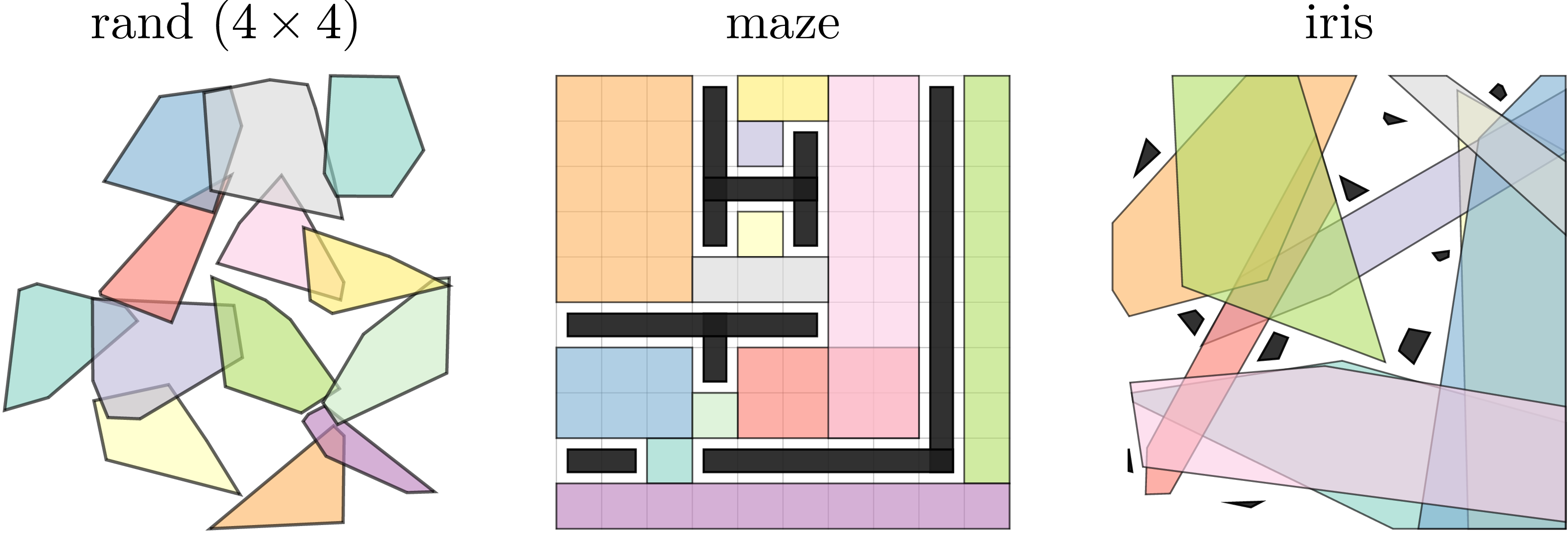
8.1 Experiment Setup↩︎
We consider three two-dimensional base domains, rand, maze, and iris, to define the problem domains for benchmarking the spatiotemporal and MRMP planners. Each ST-GCS instance initializes a seeded spatial GCS as described in Sec. 8.1.1, and then extrudes the spatial sets through time \(t\in[0,t_\mathrm{max}]\) with \(t_\mathrm{max}=1000\). We precompute the heuristics \(h_\text{tri}\) and \(h_\text{tab}\) on only these base ST-GCSs, although Sec. 8.1.2 additionally adds dynamic obstacles into each base ST-GCS instance.
8.1.1 Spatial GCS Generation↩︎
For rand, we generate an \(n \times n\) grid, sample a random convex polygon around each grid cell, connect intersecting convex sets, and retain the largest connected component. For maze, we first generate a random \(10 \times 10\) maze via recursive division [66] and then merge adjacent free cells into larger axis-aligned rectangles whenever possible using a bipartite matching procedure similar to that of [67]. For iris, we sample \(10\) polygonal static obstacles in a square workspace and grow a connected cover of collision-free convex sets with the IRIS algorithm [40]. This presents a set of more realistic GCS commonly seen in practice. The robot radius is \(0.1\) in rand, and \(0.25\) in maze and iris. Fig. 12 shows examples of the generated spatial GCS.
8.1.2 Spatiotemporal Planning Instances↩︎
We generate \(60\) single-robot spatiotemporal planning instances, with \(20\) instances from each of rand, maze, and iris. Each query is a feasible query on one seeded base ST-GCS and starts at time \(0\) with a velocity bound \(\mathbf{v}_{\mathrm{lim}}=[1.0,\ldots,1.0]\). We then add moving obstacles with piecewise-linear trajectories and the same object occupancy model as defined in Eqn. (17 ) while preserving query feasibility. The resulting ST-GCS instances have a median of \(33\) vertices and \(184\) edges.
8.1.3 MRMP Instances↩︎
We generate \(60\) MRMP instances, with \(20\) instances from each of rand, maze, and iris. Each instance contains \(n\)-robot queries on a seeded base ST-GCS, where each robot query starts at time \(0\) with a velocity bound \(\mathbf{v}_{\mathrm{lim}}=[1.0,\ldots,1.0]\). The query generation for the start positions \(\mathbf{p}_{s,1},\ldots,\mathbf{p}_{s,n}\) and goal positions \(\mathbf{p}_{g,1},\ldots,\mathbf{p}_{g,n}\) follow the assumption as in condition ([wellform:separation]), while keeping their independent trajectories still intersects to make the MRMP instances emphasize coordination rather than isolated planning.
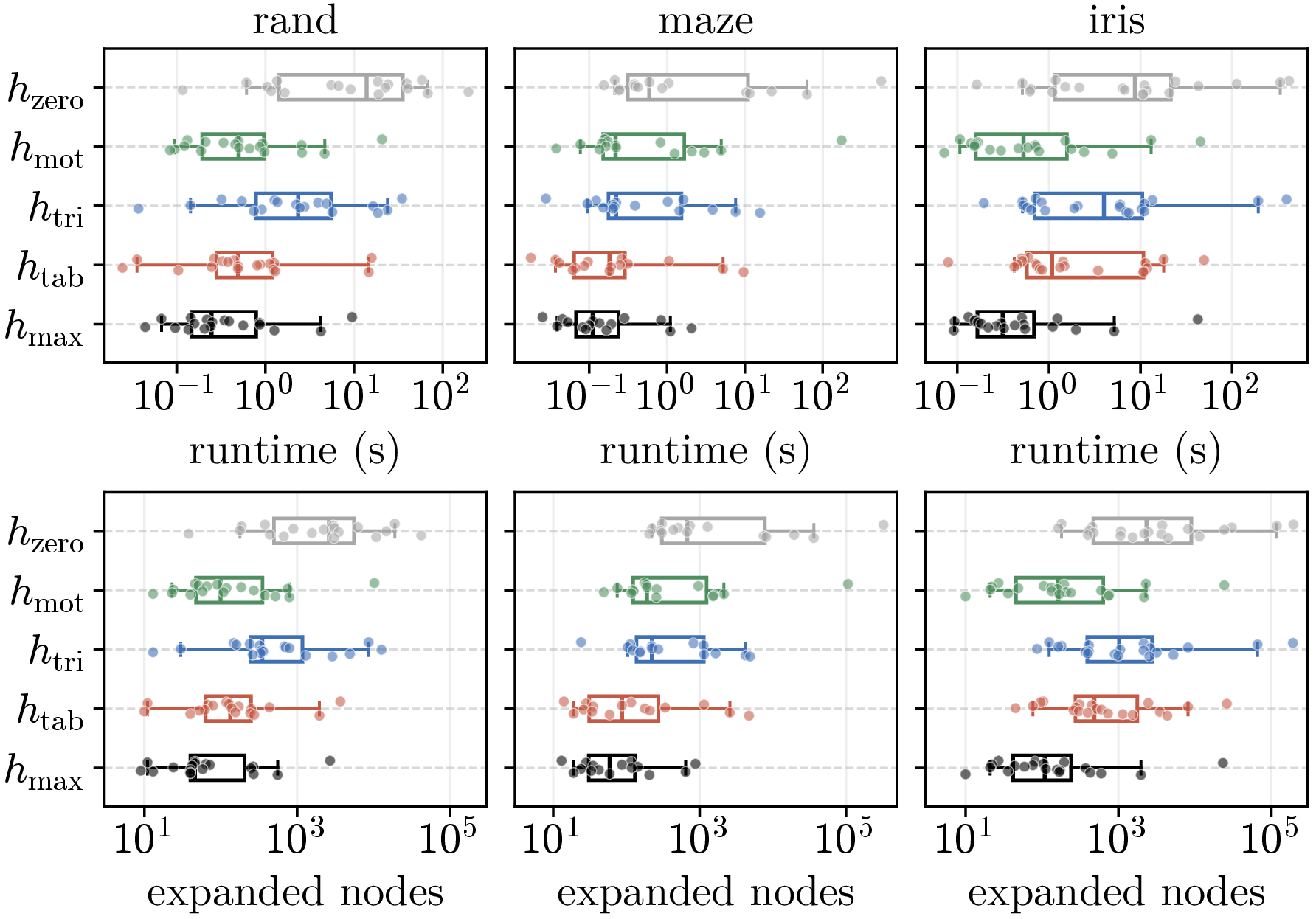
8.2 Ablation Study↩︎
This subsection follows our algorithmic stack for MRMP. We first ablate the low-level single-robot spatiotemporal planning BFS solver (Alg. 5), and then the child node expansion rules used by full-horizon PBS (Alg. 11), and at last the planning horizons in windowed coordination in Sec. 7.5. All ablation planners have a \(10\)-minute runtime budget. Unless otherwise stated, we set all their inflation factors to \(\epsilon = 1\) for the heuristics used in the low-level BFS solvers.
8.2.1 BFS Heuristics↩︎
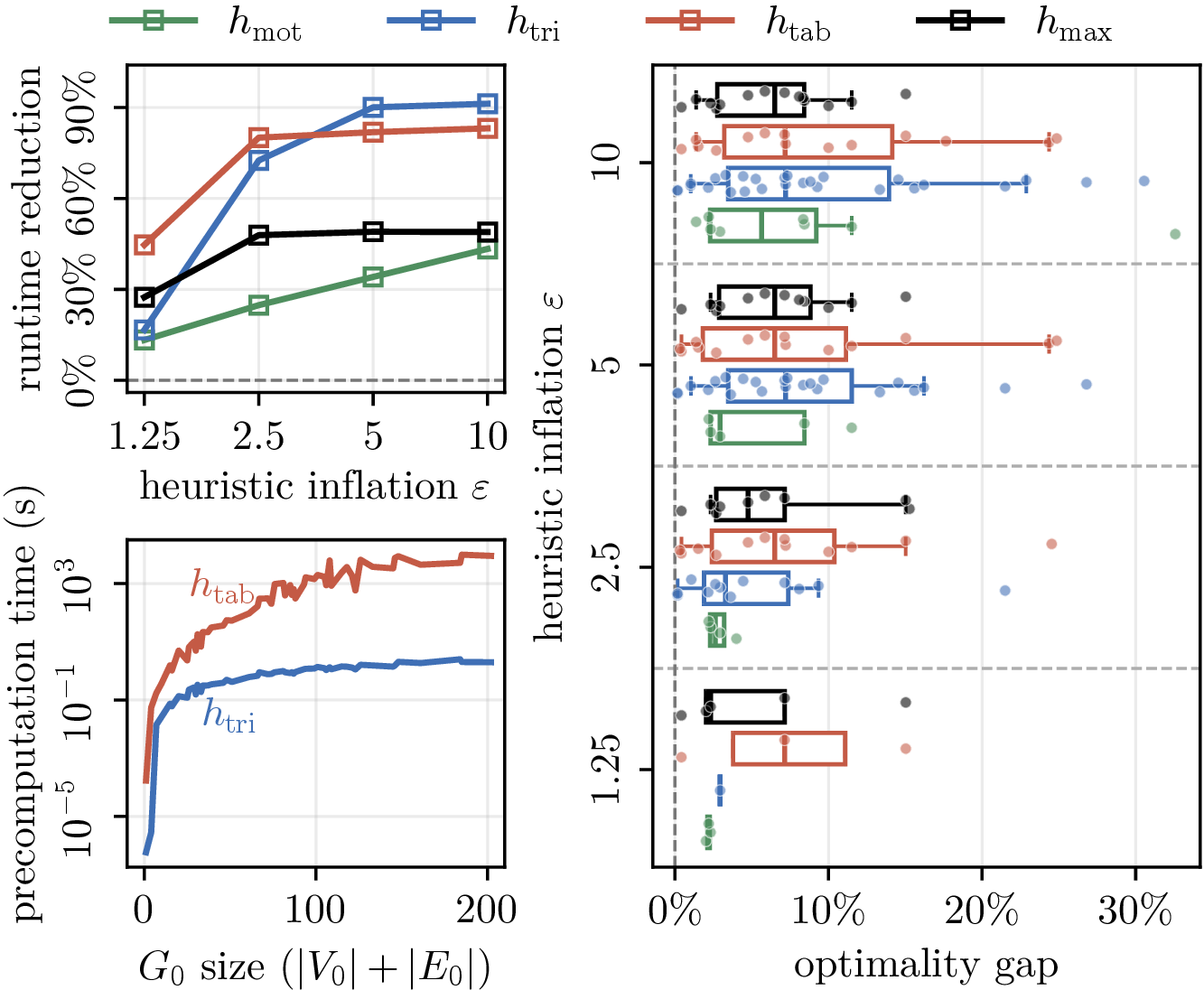
This ablation isolates the BFS heuristic (Sec. 5.5) with upper-bound pruning enabled and no optional pairwise dominance check (Sec. 5.4). Fig. 13 shows that \(h_\text{max}\) is the most robust choice. The \(h_\text{max}\) and \(h_\text{tab}\) heuristics solve all \(60\) instances in Sec. 8.1.2, while \(h_\text{mot}\), \(h_\text{tri}\), and \(h_\text{zero}\) solve \(58\), \(56\), and \(53\), respectively. On common-success instances, \(h_\text{max}\) has the smallest median runtime and expanded-node count in every domain. Relative to \(h_\text{zero}\), it reduces the median runtime by \(5.3\)–\(56.2\times\) and the median number of expanded nodes by \(11.5\)–\(56.5\times\) across the three domains. Among the single-component heuristics, \(h_\text{mot}\) is competitive on rand and strongest on the most open iris, while \(h_\text{tab}\) solves all instances and is strongest on maze, where detours make the motion-only bound less informative; \(h_\text{tri}\) is weaker without inflation. Fig. 14 shows that increasing \(\epsilon\) substantially reduces runtime, especially for \(h_\text{tri}\) and \(h_\text{tab}\), but larger inflation factors produce wider optimality-gap tails. At \(\epsilon=5\), the median runtime reductions are about \(65\%\) for \(h_\text{mot}\), \(91\%\) for \(h_\text{tri}\), \(88\%\) for \(h_\text{tab}\), and \(56\%\) for \(h_\text{max}\). The precomputation panel reports median preprocessing runtime. The \(h_\text{tri}\) heuristic stays in the seconds range, whereas \(h_\text{tab}\) requires substantially more precomputation and peaks over \(2.5\) hours. We therefore use \(h_\text{max}\) as the default BFS heuristic and inflate it when bounded suboptimality is allowed. It inherits the strongest available component lower bound at each prefix path, and its offline cost is amortized in MRMP because many low-level calls reuse the precomputation for the same base ST-GCSs.

8.2.2 BFS Dominance Checks↩︎
This ablation isolates the effect of the pairwise dominance check (Sec. 5.4) with the heuristic fixed to \(h_\text{max}\). All variants use the same upper-bound pruning, and differ only in the optional pairwise dominance check. The alternatives are the safe set-containment check \(\delta_\text{set}\), the heuristic position-based check \(\delta_\text{pos}\), and the heuristic arrival-state-containment check \(\delta_\text{state}\). The auxiliary vertex-indexed search used to obtain the incumbent contributes only the scalar upper-bound cost \(c_\text{ub}\), so differences in success, runtime, and solution cost come from the selected pairwise dominance check. Fig. 15 compares the upper-bound-only variant (UB) and the three pairwise dominance checks in runtime, expanded nodes, and solution-cost increase. UB, \(\delta_\text{set}\), and \(\delta_\text{state}\) solve all \(60\) instances in Sec. 8.1.2, while \(\delta_\text{pos}\) solves \(59\) instances. Relative to \(\delta_\text{set}\) on common-success instances, \(\delta_\text{pos}\) and \(\delta_\text{state}\) reduce the median expanded-node count by \(65.4\%\) and \(42.7\%\), and reduce the median runtime by \(41.1\%\) and \(42.1\%\), respectively. Both heuristic checks have zero median solution-cost increase over all common-success instances. \(\delta_\text{state}\) has three positive solution-cost increases, with a \(1.68\%\) median positive increase and a \(4.8\%\) worst-case increase. In contrast, \(\delta_\text{pos}\) trades more aggressive pruning for fourteen positive solution-cost increases, with a \(4.14\%\) median positive increase and a \(15.1\%\) worst-case increase. Overall, these results suggest using \(\delta_\text{pos}\) as the default scalable pairwise dominance check when small heuristic losses are acceptable, and using \(\delta_\text{state}\) when low-level success and solution quality should stay closer to the \(\delta_\text{set}\) reference.
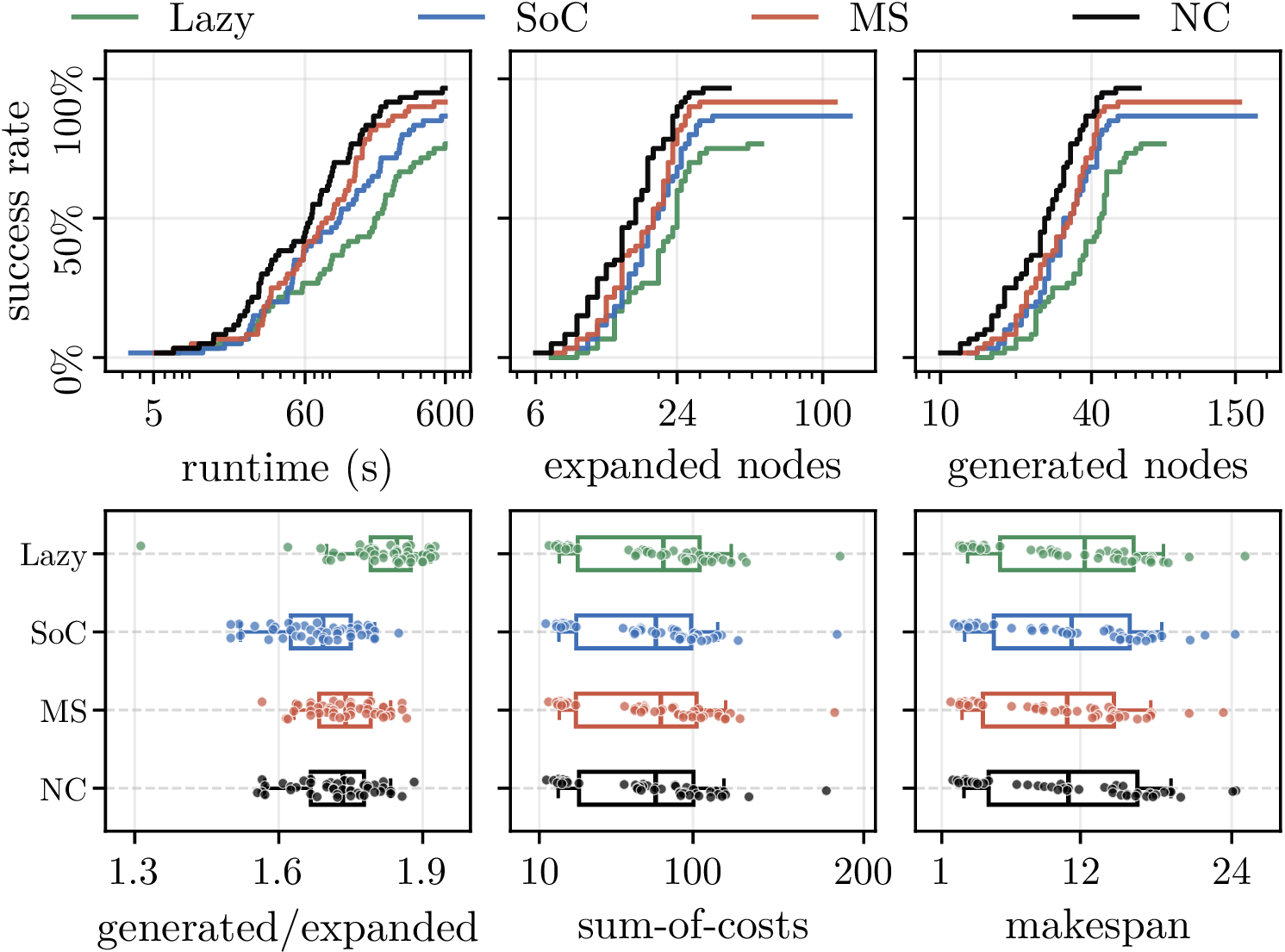
8.2.3 PBS Node Expansion Rules↩︎
This ablation isolates the node expansion rule of full-horizon PBS in Alg. 11. As introduced in Sec. 7.3.1, we compare the four rules of lazy evaluation (Lazy), the sum-of-costs (SoC) metric, the makespan (MS) metric, and the number of conflicts (NC) metric. All variants share the same low-level BFS solver with \(h_\text{max}\) heuristic, upper-bound pruning, and \(\delta_\text{pos}\) dominance check. Recall that a PBS node is said to be generated once created by adding a new partial priority order, while it is expanded once the robots are replanned via UpdateNode. As shown in the first row of Fig. 16, the NC rule gives the strongest PBS scalability on \(60\) \(10\)-robot MRMP instances generated in Sec. 8.1.3. It solves \(58\) instances within the \(600\)s budget, compared with \(55\), \(52\), and \(46\) for the MS, SoC, and Lazy rules, respectively. It also exhibits the best anytime behavior, solving \(42\) instances by \(120\)s and \(52\) instances by \(200\)s, which is consistent with the two node-count curves. We now look at the second row containing \(45\) instances solved by all four rules. The generated/expanded ratio subplot shows that the Lazy rule does postpone node expansions, with the largest ratio reaching \(1.93\) as PBS moves closest to a binary search tree. The two solution-quality subplots show that median solution-quality differences among expansion rules are modest. The NC and SoC rules have nearly tied median SoC (\(78.1\) and \(78.2\)), while Lazy and MS have higher median SoC (\(82.6\) and \(81.2\)). The MS rule gives the lowest median MS of \(10.9\), compared with at least \(11.1\) for the other rules. In general, the NC rule is suggested as the default node expansion rule because it gives the strongest scalability while remaining competitive in median SoC and MS.
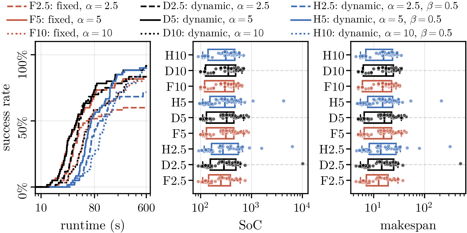
8.2.4 Windowed Coordination↩︎
This ablation isolates the planning window \(t_\text{plan}\) and the execution window \(t_\text{exec}\) for windowed-PBS as described in Sec. 7.5. We compare \(\Delta t_{\mathrm{plan}}=\alpha r/\|\mathbf{v}_{\mathrm{lim}}\|_\infty\) with a planning span factor \(\alpha\in\{2.5,5,10\}\), and \(\Delta t_{\mathrm{exec}}=\beta\Delta t_{\mathrm{plan}}\) with an execution span factor \(\beta\in\{0.5,1\}\). In addition, we compare the variants with static windows and dynamically adjusted windows as introduced in Sec. 7.5.1. All variants use \(h_\text{max}\) heuristic with inflation factor \(\epsilon=10\), upper-bound pruning, \(\delta_\text{pos}\) dominance check, and the NC child-node expansion rule on \(60\) \(20\)-robot MRMP instances generated in Sec. 8.1.3, with a \(600\)s per-instance runtime budget. Fig. 17 shows that dynamic window adjustment improves the \(\beta=1\) success count for all spans, from \(36\) to \(50\) instances at \(\alpha=2.5\), from \(50\) to \(55\) at \(\alpha=5\), and from \(49\) to \(50\) at \(\alpha=10\). Larger windows are not monotonically beneficial because they trade fewer coordination calls for harder local subproblems. Increasing \(\alpha\) from \(5\) to \(10\) raises the \(\beta=1\) median runtime from \(40.1\)s to \(65.1\)s and reduces success from \(55\) to \(50\) instances. For fixed \(\alpha\), dynamic \(\beta=0.5\) shifts the corresponding \(\beta=1\) curve toward larger runtimes. It recovers some instances missed by \(\beta=1\), but is not a strict improvement. For \(\alpha=2.5,5,10\), it gains \(5\), \(4\), and \(6\) instances while losing \(12\), \(5\), and \(2\) instances solved by the corresponding \(\beta=1\) variant. The solution-quality panels show the complementary tradeoff. Shorter windows can yield shorter successful trajectories, with fixed \(\alpha=2.5\) giving the lowest median SoC/makespan (\(250.0/12.5\)), but only \(36\) successes. Among the more reliable variants, dynamic \(\alpha=5,\beta=1\) achieves the highest success count (\(55\)) with median SoC/makespan \(325.0/16.2\). Using \(\beta=0.5\) improves median SoC/makespan for the same dynamic \(\alpha\) values, but at the cost of longer runtimes. Overall, dynamic \(\alpha=5,\beta=1\) gives the best scalability–quality tradeoff in this ablation.
8.3 Performance Comparison↩︎
This subsection presents the performance comparison results on spatiotemporal planning and MRMP.
8.3.1 Spatiotemporal Planning Benchmark↩︎
We evaluate the spatiotemporal planners under \(60\)s runtime budget on the \(60\) instances from Sec. 8.1.2. The first two are BFS variants shortlisted from previous ablations. Both use \(h_\text{max}\), upper-bound pruning, and \(\epsilon=10\), and differ only in whether they use \(\delta_\text{pos}\) or \(\delta_\text{set}\). The \(\delta_\text{pos}\) variant tests the more aggressive point-based dominance check, whereas the \(\delta_\text{set}\) variant tests set-containment pruning with the same inflated max heuristic. The optimization-based baselines are MICP and MICP(g), which solve Eqns. (6 ). MICP directly solves the program to optimality, while MICP(g) solves its linear relaxation and then applies stochastic path rounding (see Sec. 4.2) with \(\lceil 1000\log |E| \rceil\) rounded paths [7]. We also compare against the sampling-based baseline ST-RRT\(^*\) [4] from OMPL [68], reporting both the first feasible trajectory and the final incumbent solutions. Given the robot radius \(r\), we also compare against the discrete search-based Zeta\(^*\)-SIPP [11] with cell sizes of \(r\) and \(2r\).
8.3.2 Spatiotemporal Planning Scalability↩︎
Fig. 18 shows that the proposed BFS solvers on ST-GCS are the only planning variants that solve all \(60\) instances while remaining consistently subsecond. The bounded-suboptimal \(\delta_\text{set}\) variant has a \(0.10\)s median runtime, while the \(\delta_\text{pos}\) variant has a \(0.12\)s median runtime. Running the same \(\delta_\text{set}\) solver with \(\epsilon=1\) increases the median runtime to \(0.23\)s. The two optimization baselines on ST-GCS are substantially less scalable. MICP solves \(31\) instances with a \(6.03\)s median runtime on successful runs, whereas MICP(g) solves \(59\) instances with a \(1.30\)s median runtime. The non-ST-GCS baselines expose representation-dependent scalability and success behavior. For ST-RRT\(^*\), the first feasible trajectory appears on \(57\) instances with a \(0.06\)s median time-to-first-solution, but the planner reaches its final incumbent only after the full anytime budget. The domain split still shows geometry dependence, since ST-RRT\(^*\) solves all \(20\) rand and iris instances but only \(17\) maze instances. This dependence is visible in the success-rate curves. The iris instances reach \(20/20\) successes by \(0.005\)s, rand reaches \(16/20\) by \(0.47\)s and \(20/20\) only after the last successful first solution at \(8.84\)s, and maze reaches \(17/20\) by \(3.82\)s and remains below full success through \(60\)s. ST-RRT\(^*\) samples and connects directly in continuous collision-free space rather than using the GCS adjacency, so the maze domains make it harder to discover a temporally feasible connection within the budget. Zeta\(^*\)-SIPP with cell size \(r\) solves \(46\) instances with a \(0.34\)s median runtime, while the coarser \(2r\) grid solves \(41\) instances with a \(0.13\)s median runtime. Its success depends on the spatial discretization. The finer grid improves success on rand instances (\(9/20\) versus \(4/20\)), while both grids solve \(17/20\) maze instances and all \(20\) iris instances. Zeta\(^*\)-SIPP searches safe intervals only on fixed spatial grids; when the grid cells and line-of-sight edges do not represent the relevant passage, a feasible trajectory may be absent from the discretized search space.
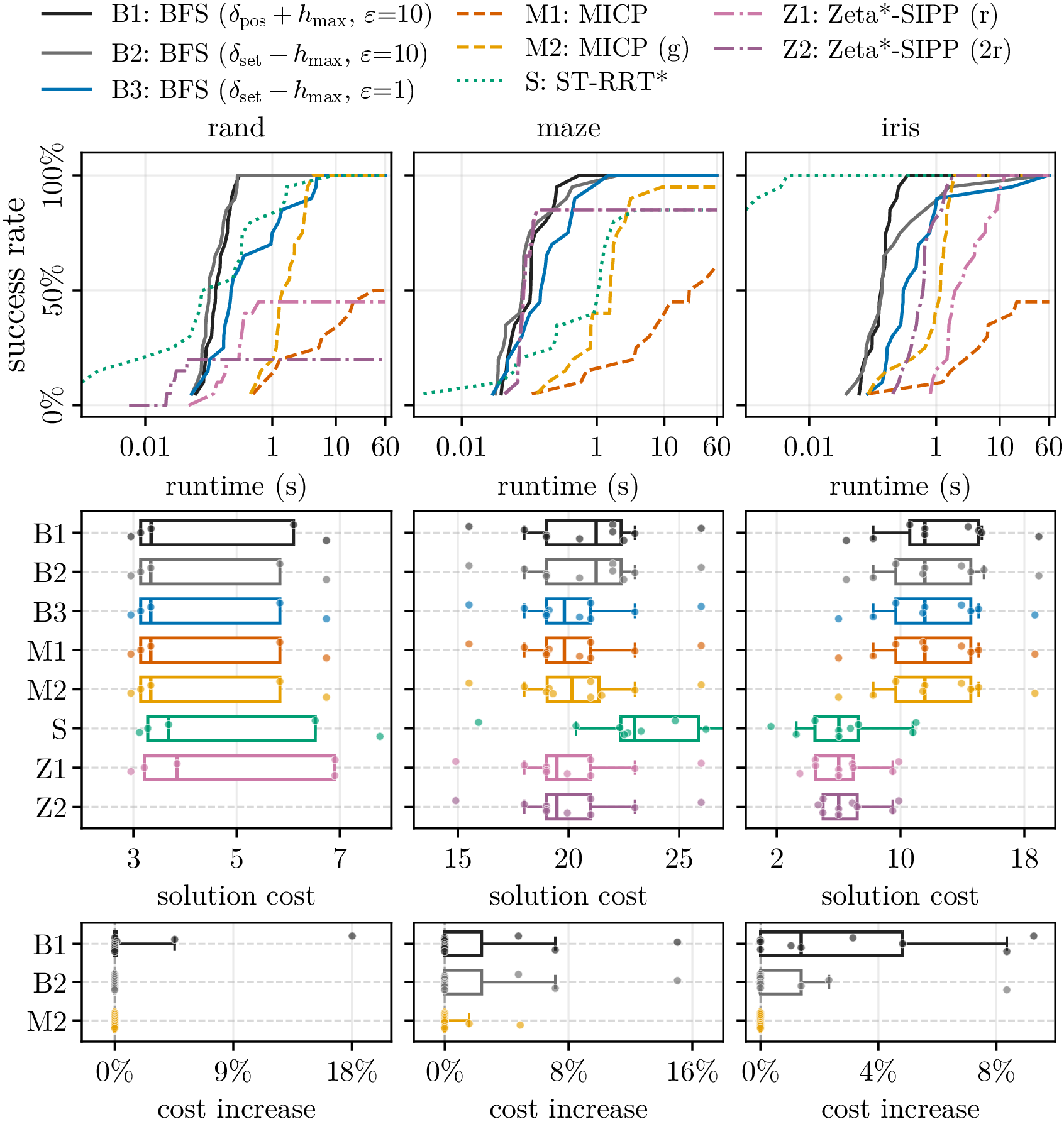
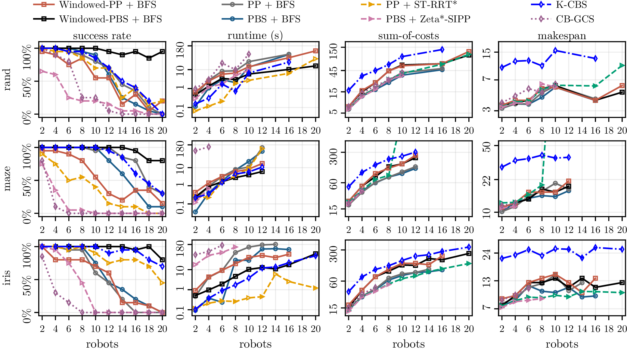
8.3.3 Spatiotemporal Planning Solution Quality↩︎
The middle and bottom rows of Fig. 18 show that the search-based ST-GCS solvers preserve solution quality while improving scalability. The bounded-suboptimal \(\delta_\text{set}\) variant has a \(9.08\) median cost, while the \(\delta_\text{pos}\) variant has a \(9.18\) median cost. Running the \(\delta_\text{set}\) solver with \(\epsilon=1\) reduces the median cost to \(8.53\), compared with a \(9.70\) median cost for MICP(g). On the \(30\) instances solved by MICP, the two inflated BFS variants, and MICP(g), the median cost increase relative to MICP is \(0.0\%\) for all three non-MICP planners. Nonzero increases occur on \(12\), \(6\), and \(2\) instances for \(\delta_\text{pos}\), \(\delta_\text{set}\), and MICP(g), respectively, with median positive increases of \(4.79\%\), \(5.95\%\), and \(3.23\%\). For the anytime ST-RRT\(^*\) baseline, the final incumbent substantially improves solution quality after the first feasible trajectory is found. Across its \(57\) successful instances, the final incumbent reduces the median successful cost from \(9.29\) to \(6.49\). The single ST-RRT\(^*\) legend entry uses first-feasibility time for success and final-incumbent cost for quality. The solution-cost comparisons should be interpreted relative to the solution space represented by each planner. For rand and maze, the ST-GCS-based planners produce costs close to the ST-GCS optimum, with small increases for the inflated BFS variants and MICP(g) on common-success instances. For iris, however, the ST-GCS-based planners generally have higher costs than the non-ST-GCS baselines. This is expected since IRIS-generated convex sets provide only partial coverage of the full collision-free space, so ST-GCS optimality is with respect to the ST-GCSs rather than the entire continuous free space.
8.3.4 MRMP Benchmark↩︎
We evaluate various MRMP planners under \(180\)s runtime budget on \(n\)-robots MRMP instances, where each \(n=2,4,\ldots,20\) corresponds to \(60\) instances generated as in Sec. 8.1.3. The proposed Windowed-PBS + BFS applies windowed-PBS with NC node expansion rule and \(\Delta_\text{plan}=\Delta_\text{exec}=5r/||\mathbf{v}_\text{lim}||_\infty\) as the high-level coordinator, and the BFS solver with \(h_\text{max}\), \(\epsilon=10\), upper-bound pruning, and \(\delta_\text{pos}\) as the low-level solver, which empirically is most scalable under limited runtime. With the same low-level BFS solver, we also compare several composed baselines with different high-level coordinators, namely, windowed-PP with \(\Delta_\text{plan}=\Delta_\text{exec}=5r/||\mathbf{v}_\text{lim}||_\infty\), PBS with NC node expansion rule, and PP. To test the alternative low-level planners in Sec. 8.3.1, we evaluate PBS + Zeta\(^*\)-SIPP with discretization of \(r\), and PP + ST-RRT\(^*\). PP + ST-RRT\(^*\) is adopted as an anytime prioritized planning baseline. After the first priority-ordered pass produces a feasible joint solution, the remaining budget is used for improvement rounds that revisit the robots in the same order and replace an incumbent trajectory only when ST-RRT\(^*\) finds a shorter collision-free trajectory against the current reservations. We report its first feasible solution for runtime and its final incumbent solution for solution quality. In addition, we compare with two standalone MRMP baselines. K-CBS [26] is a fast feasibility-oriented and sampling-based MRMP planner from OMPL [68]. CB-GCS [57] similarly solves MRMP on GCSs under a fixed time-step representation.
| \(n\) | Query Density | Runtime Total | Runtime Breakdown | |||
| Search | Opt. | ECD | Others | |||
| 2 | 19.2% | 0.41s | 50.2% | 37.2% | 0.0% | 12.6% |
| 4 | 43.7% | 1.29s | 44.6% | 36.7% | 7.8% | 11.0% |
| 6 | 52.0% | 2.67s | 41.5% | 37.7% | 10.9% | 9.9% |
| 8 | 58.5% | 4.99s | 38.3% | 38.1% | 13.9% | 9.7% |
| 10 | 65.9% | 8.04s | 35.1% | 39.3% | 16.5% | 9.2% |
| 12 | 69.5% | 12.6s | 35.3% | 39.2% | 17.4% | 8.1% |
| 14 | 71.7% | 17.7s | 33.1% | 37.7% | 20.7% | 8.6% |
| 16 | 76.4% | 25.9s | 29.5% | 39.6% | 22.5% | 8.4% |
| 18 | 78.4% | 48.9s | 28.2% | 42.1% | 22.5% | 7.2% |
| 20 | 79.1% | 40.2s | 28.9% | 40.6% | 22.9% | 7.6% |
3.5pt
8.3.5 MRMP Scalability↩︎
Fig. 19 shows that the proposed Windowed-PBS + BFS has the highest success rate. Over the \(n\ge 10\) instances, it solves \(338\) out of \(360\) instances. All baselines solve fewer cases in the same regime. Among the other composed baselines, PP + BFS solves \(159\), PP + ST-RRT\(^*\) solves \(151\), PBS + BFS solves \(135\), Windowed-PP + BFS solves \(108\), and PBS + Zeta\(^*\)-SIPP solves \(9\). The two standalone baselines also degrade at high robot counts. K-CBS solves \(242\) instances for \(n\ge 10\), while CB-GCS solves only \(6\). At \(n=20\), Windowed-PBS + BFS solves \(19/20\) rand, \(16/20\) maze, and \(16/20\) iris instances, giving \(51/60\) successes overall. The next-best baseline at this scale is K-CBS with \(20/60\) successes. The remaining baselines solve \(13/60\) cases for PP + ST-RRT\(^*\), \(7/60\) for Windowed-PP + BFS, \(6/60\) for PP + BFS, \(2/60\) for PBS + BFS, and \(0/60\) for PBS + Zeta\(^*\)-SIPP and CB-GCS. These comparisons separate the two ingredients needed for scalability. Windowing alone is not sufficient. Windowed-PP + BFS uses the same low-level solver and horizon schedule as Windowed-PBS + BFS, but solves only \(108/360\) high-count cases and \(7/60\) cases at \(n=20\). PBS alone is also not sufficient. Full-horizon PBS + BFS solves \(135/360\) high-count cases and only \(2/60\) cases at \(n=20\). The proposed combination avoids these two failure modes by resolving local priority conflicts inside each window while committing only the next execution interval. The comparison against PP + ST-RRT\(^*\) and K-CBS is clearest on the most challenging \(n\ge 16\) instances. Windowed-PBS + BFS solves \(55/60\), \(51/60\), and \(55/60\) cases on rand, maze, and iris, respectively. PP + ST-RRT\(^*\) solves \(15/60\), \(2/60\), and \(39/60\), while K-CBS solves \(12/60\), \(27/60\), and \(49/60\). On successful runs in this regime, the median runtimes of Windowed-PBS + BFS are \(37.1\)s, \(20.8\)s, and \(51.9\)s across the three domains. PP + ST-RRT\(^*\) has successful-run median runtimes of \(15.1\)s, \(88.5\)s, and \(1.07\)s, while K-CBS has \(105\)s, \(82.3\)s, and \(37.1\)s. Thus, although PP + ST-RRT\(^*\) and K-CBS are very strong baselines on smaller instances with fewer robots, the proposed Windowed-PBS + BFS remains the only scalable choice for the most challenging MRMP instances across all three domains. Tab. 1 shows search and optimization dominate the runtime, while ECD becomes substantial at larger \(n\) and other costs remain small. The query density reports the area fraction of the entire spatial GCSs covered by the union of the start and goal hypercube occupancies as in Eqn. (16 ).
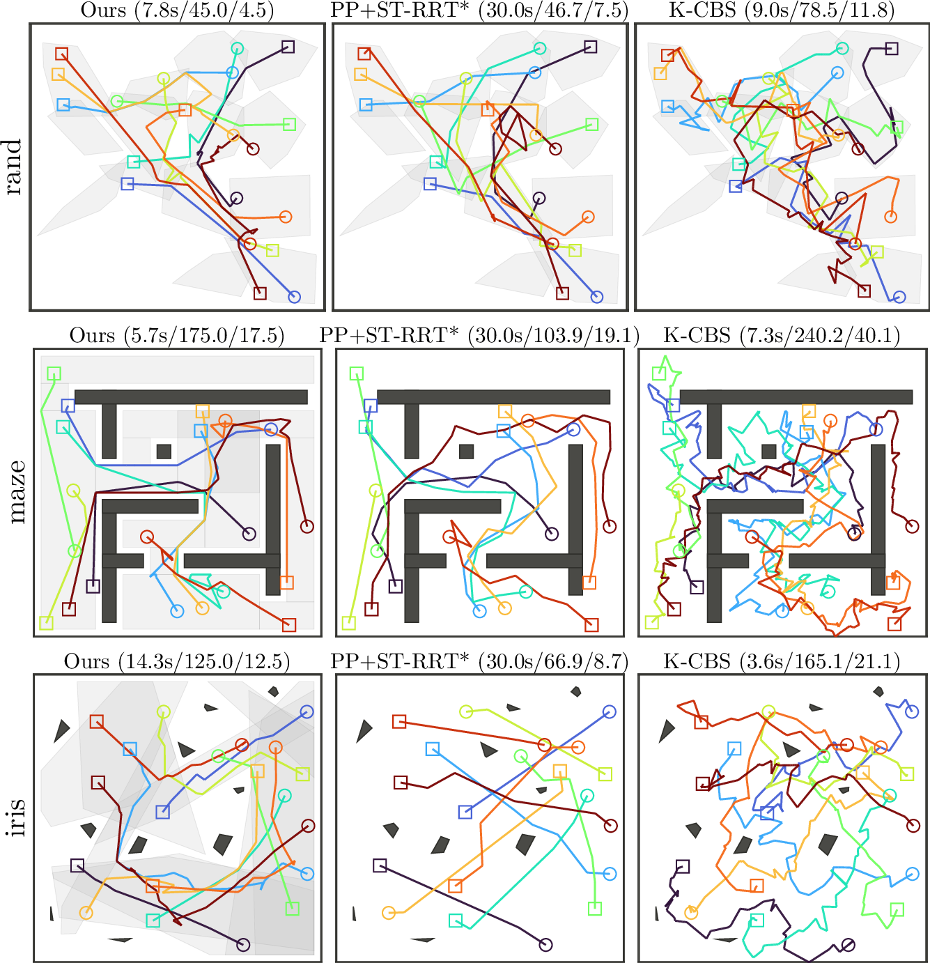
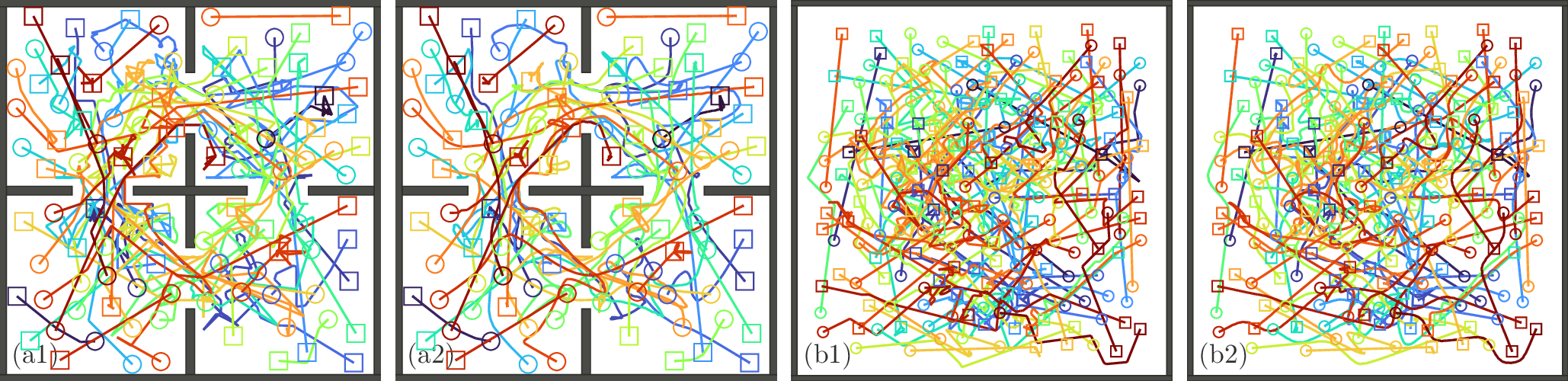
8.3.6 MRMP Solution Quality↩︎
The SoC and makespan rows of Fig. 19 show that the proposed Windowed-PBS + BFS retains competitive solution quality while achieving the scalability reported above. We report the median SoC and makespan on the \(n\le 10\) instances where most planners succeed on substantial subsets. On the corresponding common-success subsets, the median SoC/makespan Windowed-PBS + BFS is \(40.0/10.0\). Full-horizon PBS + BFS and PP + BFS have lower median SoC/makespan \(26.7/8.71\) and \(27.3/8.79\), respectively. Windowed-PP + BFS gives a similar limited-horizon tradeoff, with median SoC/makespan \(40.0/10.0\). Thus, windowed coordination sacrifices some SoC since it plans and commits only within a finite horizon, while keeping the makespan close to the full-horizon BFS planners. In contrast, the feasibility-oriented K-CBS has substantially worse solution quality with median SoC/makespan \(66.0/21.7\). PP + ST-RRT\(^*\) is a stronger solution-quality baseline in favorable domains after using the full \(180\)s runtime budget. On iris, it achieves median SoC/makespan \(33.6/8.33\), below the median \(60.0/10.0\) of Windowed-PBS + BFS. As in Sec. 8.3.3, this gap is expected since IRIS-generated convex sets only partially cover the full collision-free space. However, its quality advantage is domain-dependent. On maze, PP + ST-RRT\(^*\) has median SoC/makespan \(42.6/15.0\), while Windowed-PBS + BFS has median SoC/makespan \(60.0/14.4\). Fig. 20 illustrates these domain-dependent quality differences on representative \(10\)-robot examples with a 30s runtime budget. Overall, K-CBS emphasizes feasibility at the cost of longer joint plans. PP + ST-RRT\(^*\) can produce high-quality solutions in favorable domains but is less consistent. Windowed-PBS + BFS provides the most consistent quality-scalability tradeoff across domains.
9 Applications and Demonstrations↩︎
This section complements the quantitative comparisons above with several demonstration scenarios. We first describe a trajectory-optimization postprocessing step for smoothing the piecewise-linear trajectories produced by our planner, then demonstrate the solutions on large-scale simulated problems and real-robot deployments.

9.1 Global Trajectory Optimization↩︎
The proposed MRMP planner produces piecewise-linear trajectories with fixed vertex paths on ST-GCS. As a postprocessing step, we can smooth these trajectories by solving a Quadratic Program (QP) over sampled spatial positions along the trajectories at fixed time samples. Given \(n\) robot trajectories \(\mathcal{T}^0=\{\tau_i^0\}_{i=1}^{n}\), we choose a shared ordered sample sequence \(\mathcal{K}=\langle t_1,\ldots,t_l\rangle\), with \(t_1<\cdots<t_l\), formed from a uniform time grid together with the original trajectory knot times. We will use \(k\) to denote the index of the fixed time sample \(t_k\).
Let \(\bar{\mathbf{p}}_{i,k}=\tau_i^0(t_k).\mathbf{p}\) be the reference position of robot \(i\) at time \(t_k\). The program keeps the times fixed and optimizes only the sampled spatial positions \(\mathbf{p}_{i,k}\in\mathbb{R}^{m}\). Similarly to Sec. 7.1, we assume a common radius \(r\) for the robots. For compactness, we define the sampled velocity and velocity-variation term as follows: \[\begin{align} \mathbf{v}_{i,k}(\mathbf{p}) &= \frac{\mathbf{p}_{i,k+1}-\mathbf{p}_{i,k}}{t_{k+1}-t_k},\\ \mathbf{g}_{i,k}(\mathbf{p}) &= \frac{\mathbf{p}_{i,k+1}-\mathbf{p}_{i,k-1}}{t_{k+1}-t_{k-1}} - \frac{\mathbf{p}_{i,k}-\mathbf{p}_{i,k-2}}{t_k-t_{k-2}}. \end{align}\] Let \(\mathcal{F}_i\) denote the samples at which robot \(i\) is fixed at its initial or terminal state. For each interval \([t_k,t_{k+1}]\), let \(v_{i,k}\) be the ST-GCS vertex traversed by the input piecewise-linear trajectory at the interval midpoint. We formulate the trajectory optimization as: \[\begin{align} \min_{\{\mathbf{p}_{i,k}\}}\quad &\sum_{i=1}^{n}\Big(\lambda_{c}\sum_{k=3}^{l-1} \|\mathbf{g}_{i,k}(\mathbf{p})\|_2^2 + \lambda_{d}\sum_{k=1}^{l} \|\mathbf{p}_{i,k}-\bar{\mathbf{p}}_{i,k}\|_2^2\Big) \notag\\ \boldsymbol{s.t.}\quad & \mathbf{p}_{i,k}=\bar{\mathbf{p}}_{i,k}, \tag{21}\\ & -\mathbf{v}_{\mathrm{lim}}\preceq \mathbf{v}_{i,k}(\mathbf{p}) \preceq \mathbf{v}_{\mathrm{lim}}, \tag{22}\\ & (\mathbf{p}_{i,k},t_k),\,(\mathbf{p}_{i,k+1},t_{k+1}) \in X_{v_{i,k}}, \tag{23}\\ & \mathbf{n}_{ij,k}^{\top}(\mathbf{p}_{i,k}-\mathbf{p}_{j,k}) \geq 2r, \tag{24} \end{align}\] where Eqns. (21 )–(23 ) are enforced for every robot and all valid sample indices, with Eqn. (21 ) restricted to \(k\in\mathcal{F}_i\). Eqn. (24 ) is enforced for every robot pair \(1\leq i<j\leq n\) and every sample \(k\). The objectives regularize velocity variation and penalize deviations from the input reference trajectories. The two nonnegative weights \(\lambda_{c}\) and \(\lambda_{d}\) tune the relative emphasis of these two objective terms, respectively. Eqn. (21 ) preserves the prescribed start and goal positions. Eqn. (22 ) enforces the same component-wise velocity limits constraint as Eqn. (12 ) in the original formulation. Eqn. (23 ) constrains both endpoints of each optimized segment to lie in the same set \(X_{v_{i,k}}\) of the original trajectory segment. Since each optimized segment is a linear interpolation in space-time between the two endpoints, the convexity of \(X_{v_{i,k}}\) keeps the entire optimized segment inside this collision-free set. Eqn. (24 ) is a sampled linearization of pairwise robot separation, where \(\mathbf{n}_{ij,k}=(\bar{\mathbf{p}}_{i,k}-\bar{\mathbf{p}}_{j,k})/\|\bar{\mathbf{p}}_{i,k}-\bar{\mathbf{p}}_{j,k}\|_2\) is the unit normal precomputed from the original sampled positions \(\bar{\mathbf{p}}_{i,k}\) and \(\bar{\mathbf{p}}_{j,k}\) at time \(t_k\).
When explicit obstacle representations are available, we can further replace Eqn. (23 ) with direct sampled collision-avoidance constraints. At each sample time \(t_k\), a static obstacle uses its fixed spatial geometry, while a space-time obstacle uses its spatial slice at \(t_k\). For each robot \(i\), obstacle \(o\), and time sample \(t_k\), let \(\mathbf{a}_{i,k,o}\in\mathbb{R}^{m}\) and \(b_{i,k,o}\in\mathbb{R}\) jointly define a precomputed separating halfspace that contains the original trajectory sample \(\bar{\mathbf{p}}_{i,k}\) and excludes the obstacle geometry inflated by the robot radius \(r\). We enforce the corresponding sampled collision-avoidance constraint \(\mathbf{a}_{i,k,o}^{\top}\mathbf{p}_{i,k}\geq b_{i,k,o}\), which keeps the optimized sample on the same collision-free side of this halfspace.
The resulting smoothed trajectories are certified to be space-time collision-free only at the sampled states \((\mathbf{p}_{i,k},t_k)\) where the QP constraints are imposed. For larger instances, we improve scalability with a sequential rolling-horizon variant that optimizes a short block of consecutive time samples, fixes the accepted prefix, advances the block, and repeats until all samples have been processed. This decomposition keeps each local trajectory-optimization QP small and makes the full problem easier to solve, while retaining the same smoothing objective and sampled-state collision-free.
9.2 Large-Scale Coordination↩︎
We demonstrate in large-scale MRMP instances that the proposed Windowed-PBS + BFS planner scales to confined and highly congested workspaces, with trajectory optimization applied afterward as a smoothing post-processing step. Fig. 21 shows two planar coordination settings with complementary sources of difficulty. Using the same query-density metric as Tab. 1, the \(50\)-robot and \(100\)-robot instances have query densities of \(95.7\%\) and \(77.1\%\), respectively. In the \(50\)-robot four-room instance, the workspace funnels traffic through narrow inter-room passages, so difficulty comes from geometric bottlenecks and the need to sequence many robots through shared doorways. In the \(100\)-robot empty-workspace instance, the independent trajectories of \(97\) robots are involved in collisions initially in one connected conflict component, so difficulty comes from dense pairwise interaction rather than static obstacles. These results show that the planner remains practical both when difficulty comes from geometric bottlenecks and when it comes from dense pairwise robot interactions. Fig. 22 further stresses coordination with a \(32\)-UAV position-exchange problem on a 3D sphere, where every robot conflicts with any other robots at the sphere center. This fully coupled exchange forces the coordinator to resolve simultaneous conflicts in 3D before trajectory optimization smooths the resulting paths. Fig. 23 further tests a \(48\)-UAV instance in a fastpathplanning-style 3D village with dense buildings and trees [44]. The generated village occupies an \(8\times 8\times 3\) workspace, includes building footprints together with randomly placed tree and bush obstacles, and decomposes the remaining free space into \(119\) convex boxes. The start–goal pairs are sampled as long-distance trips across this fragmented free space, so many UAVs must simultaneously route around vertical clutter while avoiding one another in narrow local passages.
9.3 Mobile Robots Deployment↩︎
We validate our MRMP planner in an open indoor environment with a system of \(9\) differential drive mobile robots. The system is centrally controlled by an Intel Core Ultra 5 125U laptop with 16GB RAM, ROS2 Humble [69], and Vicon [70] for robot localization. Each robot has a bounding radius of 7cm and is exposed to a velocity command \((v,\omega)\), with linear velocity \(v\in [0, 0.6]\) m/s and angular velocity \(\omega\in[-2.5, 2.5]\) rad/s. Note that this velocity limit is set conservatively smaller than the physical robot limits for system robustness.
We construct a rearrange task consisting of a sequence of MRMP queries within a 3m\(\times\)3m bounding square. The goal positions in each query consecutively form a configuration of five letters: S, T, G, C, and S. All the robots start simultaneously from their previous goal configurations; specifically, they initialize and terminate in a \(3\times 3\) grid configuration. We first compute piecewise-linear solution trajectories via Windowed-PBS+BFS, and then smooth them via the trajectory optimization described in Sec. 9.1. The safe clearance between the robots is set to \(20\)cm during planning, which is \(6\)cm larger than twice the robot radius. The offline planning for the entire task took 16.28s.

During online execution, the smoothed trajectories are discretized with a \(0.05\)s time step into time-indexed waypoints, and the tracker precomputes segment-wise reference linear and angular velocities from consecutive samples. All robots receive a common start time and evaluate their own trajectory at a system-wide shared elapsed time, preserving the simultaneity encoded by the offline solution. We use a simple trajectory tracking controller for the robots with a 60-Hz frequency. In each control cycle, the tracker first identifies the active trajectory segment whose time interval contains the system time. The final published velocity command combines the active segment’s reference velocities as feedforward terms with body-frame feedback corrections computed from the interpolated desired pose error. In our deployments, the conservative velocity limits and additional planned inter-robot clearance provided enough margin for the observed tracking errors, and the robots completed the rearrangement without inter-robot collisions. Fig. 24 demonstrates the actual robot trajectories during the rearrange task.
10 Conclusions↩︎
We presented ST-GCS as a continuous-space framework for time-optimal spatiotemporal motion planning with dynamic obstacles and multi-robot interactions. By searching over path-indexed states on space-time convex sets, the proposed solver avoids a single large mixed-integer formulation while still optimizing continuous trajectories along candidate paths. The ECD scheme further allows planned occupancies to be reserved directly in the graph, enabling prioritized and windowed coordination for MRMP. Experiments show that the resulting planners substantially improve scalability while maintaining competitive solution quality. Large-scale demonstrations further show practical coordination of up to \(100\) robots within a few minutes.
Several scope limitations suggest natural directions for future work. First, the current ST-GCS formulation uses piecewise-linear trajectory representations with time monotonicity and component-wise velocity bounds, motivating richer trajectory representations for nonholonomic systems, kinodynamic constraints, and manipulation tasks. Second, this work targets offline MRMP with known environments, motivating online MRMP with frequent replanning under changing environments or lifelong task assignments, together with adaptive or approximate convex decompositions that keep such replanning more efficient. Third, finite-window coordination is incomplete in general because conflicts outside the current window are deferred, motivating stronger window-selection rules with completeness guarantees.
Funding↩︎
This work was supported by the NSERC under grant number RGPIN2020-06540 and a CFI JELF award.
References↩︎
Corresponding author email: jingtao_tang@sfu.ca↩︎