BT-APE: A Computationally Light Backtracking Approach to Automatic Prompt Engineering for Requirements Classification
July 01, 2026
Abstract
Large language models (LLMs) are increasingly applied to requirements engineering (RE) tasks, including requirements classification, model generation, trace-link detection and others. Prompts, which guide LLM behavior, are typically designed manually through trial and error, often leading to inconsistent and suboptimal performance on RE tasks. Despite the importance of prompt design, prior RE research largely relies on manually constructed prompts and does not systematically optimize them; moreover, automated methods for prompt construction remain largely unexplored, leaving their effectiveness unclear. To address this gap, we propose a lightweight Automatic Prompt Engineering (APE) approach named Backtracking APE (BT-APE) and apply it to requirements classification as a representative RE task. We frame prompt design as an optimization problem and iteratively refine prompts using LLM-generated candidates, backtracking search, and dynamic example selection. We evaluate BT-APE on three benchmark datasets with five instruction-tuned LLMs against four classical prompting baselines (zero-shot, few-shot, chain-of-thought, and CoT+few-shot) and a state-of-the-art, yet more resource intensive, APE baseline (PE2). Our results show that BT-APE and PE2 achieve nearly identical performance, both substantially outperforming the four classical prompting baselines across datasets and models, with large effect sizes. However, compared with PE2, BT-APE imposes a substantially lighter computational footprint, consuming approximately 72% fewer cumulative input tokens and 66% less wall-clock time at equivalent accuracy (see Appendix sec:sec:sec:efficiency?), making it better suited to deployment on small or resource-constrained servers. We also find that domain-informed prompt definitions enhance early performance, while iterative optimization partly compensates for weaker initial prompts. The contribution of this work is threefold: (i) a lightweight APE framework, together with an open interactive tool and replication package that operationalize the full pipeline; (ii) a comprehensive empirical evaluation across datasets and instruction-tuned LLMs that provides the first systematic comparison of APE against classical prompting for requirements classification; and (iii) insights into the impact of class definitions and prompt evolution on classification performance.
<ccs2012> <concept> <concept_id>10010147.10010178.10010179.10010182</concept_id> <concept_desc>Computing methodologies Natural language generation</concept_desc> <concept_significance>500</concept_significance> </concept> <concept> <concept_id>10011007.10010940</concept_id> <concept_desc>Software and its engineering Software organization and properties</concept_desc> <concept_significance>300</concept_significance> </concept> </ccs2012>
1 Introduction↩︎
Recent advances in Large Language Models (LLMs) are transforming Requirements Engineering (RE) [1], [2]. These models support tasks such as requirements elicitation, traceability, validation, and specification generation [3], [4]. Their effectiveness stems from large-scale pretraining and their ability to follow natural language instructions through in-context learning, without requiring task-specific training [2]. This capability is well suited to RE, where annotated data is often scarce, domain-specific, and costly to obtain, making traditional supervised approaches difficult to scale [5].
Interaction with LLMs is mediated through prompts, which are natural language instructions that guide model behavior and shape outputs [6]. Prompt quality directly affects performance, making prompt engineering a critical factor in LLM-based solutions [7]. However, in RE research, prompt design is typically manual and relies on iterative trial-and-error [2]. This process is often ad hoc and unsystematic, depends heavily on practitioner intuition, and is rarely documented in a reproducible manner [7]. As a result, it limits reproducibility and leads to inconsistent or suboptimal results across RE tasks and datasets [2].
Despite its importance, prompt engineering in RE remains underexplored [8], [9]. Existing studies rely on static prompting strategies—zero-shot, few-shot, and chain-of-thought—whose effectiveness is known to be highly sensitive to phrasing, ordering, and example selection [6]. Because these prompts are manually crafted and never updated in response to model behavior, they underutilized LLM capabilities. In contrast, recent work in the broader Natural Language Processing (NLP) literature introduces Automatic Prompt Engineering (APE) techniques that iteratively generate, evaluate, and refine prompts [10]–[13]. These approaches frame prompt design as a search or optimization problem and have demonstrated strong performance improvements across a range of tasks [14]. However, their applicability to domain-specific RE problems, where terminology, structure, and ambiguity differ from general NLP benchmarks, remains unclear.
Our prior short contribution introduced APE to RE and provided initial evidence that automated refinement can outperform standard prompting for requirements classification [15]. The preliminary study proposed a basic APE approach, focused on a single dataset and a single model, and did not analyze the effects of datasets, LLMs, or prompt design factors. This paper builds upon this study, by proposing a novel, more refined—yet lightweight—APE framework, named Backtracking-APE (BT-APE), and conducting a systematic empirical evaluation across multiple datasets and LLMs.
The proposed BT-APE framework iteratively refines prompts using LLM-generated candidates, a backtracking search strategy, and dynamic example selection. We evaluate the effectiveness of the framework in RE and identify the factors that influence its performance. We focus on requirements classification as a representative RE task [16]. The task assigns labels to textual requirements, such as functional or non-functional categories. It supports downstream activities, including requirements analysis, prioritization, and quality assurance, it is the most frequently addressed task in NLP for RE research [5], and it has been shown to be highly relevant for industrial applications [17], [18]. The task also provides a controlled setting to assess the impact of prompt design on model behavior, given the availability of multiple benchmarks. We evaluate the approach on three benchmark datasets PROMISE [19], PROMISE-Refined [20], and SecReq [21] using five instruction-tuned LLMs in the 7–8B parameter range: Qwen2-7B, Falcon3-7B, Granite-3.2-8B, Ministral-8B, and LLaMA-3-8B. We deliberately focus on instruction-tuned variants because BT-APE relies on the model’s ability to follow natural-language meta-prompts that ask it to revise an existing prompt conditioned on labelled feedback. We restrict the comparison to the 7–8B parameter range so that all models can be hosted locally on a single commodity GPU, reflecting the practical RE setting in which requirements confidentiality discourages reliance on hosted proprietary APIs. Furthermore, we analyse how prompt components, such as class definitions and examples, evolve during optimisation.
Our results show that BT-APE outperforms standard prompting strategies, and reaches performance that are equivalent with another, more resource consuming, state-of-the-art baseline method, i.e., PE2 [12], also generalizing across datasets and models. We also show that domain-informed, carefully engineered prompts improve early performance, while iterative optimization compensates for weaker initial prompts, confirming the effectiveness of BT-APE especially in scenarios where expert-crafted prompts are unavailable or difficult to design. We also observe that effective prompts share a recognizable profile: they tend to be concise and action-oriented (higher verb count), structurally clear (more punctuation markers), and lexically focused, whereas length, lexical diversity, and syntactic complexity correlate negatively with performance.
This paper makes three contributions:
The first systematic evaluation of APE on requirements classification, comparing two single-trajectory APE methods against four classical prompting strategies across three datasets and five LLMs. We show that APE transfers to RE with large effect sizes over classical prompting.
Evidence that two structurally different APE designs — PE2’s history-conditioned proposals and our BT-APE’s bounded-backtracking with balanced example batches — converge to statistically indistinguishable accuracy. We characterize the operational trade-offs (per-iteration context size, search behavior, hyperparameter interpretability) that differentiate them.
An analysis of prompt-feature evolution under BT-APE that identifies lexical, syntactic, and semantic correlates of high-performing prompts.
In addition, we release a GUI-based interactive tool that operationalises the full BT-APE pipeline, enabling practitioners to apply and experiment with the method on their own requirements classification tasks without prior expertise in prompt engineering or LLM tooling (described in Appendix 12). The tool, datasets, prompts, optimisation traces, and evaluation scripts are released as a publicly available replication package on Zenodo [22].
To support the reproducibility and extensibility of this study, additional materials are provided in the appendices. Appendix 9 presents a hyperparameter sensitivity analysis and convergence dynamics for the backtracking mechanism, characterizing the influence of patience thresholds and iteration horizons. Appendix 10 details the PE2 baseline implementation, highlighting its structural differences from our BT-APE method. Appendix 11 provides a comprehensive computational efficiency and token overhead comparison between BT-APE and PE2. Appendix 12 describes an interactive tool that operationalizes the full optimization pipeline. Appendix 13 outlines a preliminary analysis of potential data leakage using Jaccard similarity, showing that mean similarity between LLM-generated requirement continuations and ground-truth texts remains low (\(0.10\)–\(0.16\)) across all five models, with no statistically significant difference between PROMISE and SecReq.
1.0.0.1 Relation to the preliminary version.
This article substantially extends our REFSQ 2025 research preview [15], which introduced APE to requirements classification as a single-dataset, single-model proof of concept without statistical analysis. Beyond the contributions listed above, the present work (i) refines the original procedure into BT-APE by adding bounded backtracking with an explicit patience threshold, a balanced four-tuple dynamic example selection mechanism, and 3-run majority-voted evaluation; (ii) broadens the empirical scope from one dataset and one LLM to three datasets and five instruction-tuned LLMs, and adds PE2 [12] as a state-of-the-art APE baseline; (iii) replaces descriptive evaluation with a full inferential design (Wilcoxon signed-rank tests, Friedman tests with power analysis, and a linear mixed-effects model with trajectory-level random intercepts); (iv) introduces two research questions absent from the preview — the analysis of prompt-feature evolution (RQ3) and the comparison of informed vs.uninformed class-definition initialisation (RQ4); and (v) releases an interactive GUI-based tool, a hyperparameter sensitivity analysis, a computational-efficiency comparison with PE2, and a data-leakage probe based on Jaccard similarity.
The remainder of this paper is organized as follows. Section 2 introduces background and terminology. Section 3 presents the proposed approach. Section 4 describes the research design. Section 5 reports the results. Section 6 discusses the findings. Section 7 outlines threats to validity. Section 8 concludes the paper.
2 Background and Related Works↩︎
2.1 Traditional and Pre-trained Machine Learning for Requirements Classification↩︎
Requirements classification, assigning predefined labels to natural language requirements, is a foundational RE task. Typical formulations distinguish functional from non-functional requirements, sort non-functional requirements into sub-types such as performance, security, and usability, and flag security-relevant requirements [19], [21], [23]. Automating this work matters because manual classification of large requirements documents is both impractical and error-prone.
Early approaches leaned on traditional NLP and hand-crafted features—term frequency, bag-of-words, and syntactic parsing—paired with classifiers such as support vector machines and Naïve Bayes [19], [23]. These pipelines demanded heavy preprocessing and domain-specific feature design, which limited their portability across datasets and domains [5], [24].
The arrival of transfer learning with pre-trained language models shifted the picture: Hey et al. [25] proposed NoRBERT, applying BERT-based transfer learning to achieve strong results on the PROMISE dataset across binary and multi-class tasks; Dalpiaz et al. [20] contributed refined PROMISE annotations and explored interpretable models using dependency-parsing features; and Alhoshan et al. [26] showed that pre-trained models can classify requirements with no task-specific training data, albeit with a measurable gap relative to supervised baselines. Addressing the natural variance and instability inherent to individual language architectures, Alsanoosy [27] unified these classic deep learning threads by implementing an ensemble learning framework across seven distinct models (including BERT and RoBERTa).
2.2 LLMs and In-Context Learning↩︎
Modern LLMs are transformer-based networks trained on large text corpora through self-supervised objectives, and models in the GPT family represent the current state of the art across classification, summarization, translation, and code generation, frequently without task-specific fine-tuning [28]. The property that most distinguishes these models from earlier neural approaches is in-context learning: given a natural language prompt containing instructions and, optionally, a handful of demonstrations, the model produces appropriate outputs without any parameter updates. This makes LLMs especially appealing for RE, where labeled datasets tend to be small and tightly bound to a particular domain [29]. Because state-of-the-art models contain hundreds of billions of parameters and are typically reached through hosted inference APIs rather than fine-tuned locally, the practical lever available to most RE researchers is no longer the model’s weights but the text of the prompt itself [9]. Within RE, LLMs have been applied well beyond classification—to elicitation, validation, traceability, and specification generation [29]–[31]. Ferrari et al. [29] explored generating UML sequence diagrams from requirements, while Rodriguez et al. [30] studied how prompt design shapes automated software traceability. Recently, SLMs are increasingly preferred over LLMs due to their efficiency and competitive performance on specialized tasks [4], [32]. Studies have shown that SLMs can match or even outperform LLMs in domain-specific applications such as requirements classification, while also significantly reducing computational and energy costs [33], [34].
2.3 LLMs in Requirements Classification↩︎
Recent work on requirements classification has moved from traditional machine learning and encoder-based baselines toward LLM-based approaches. Santos et al. [31] report that few-shot and zero-shot prompting with GPT-4 and open-source models can approach the performance of fine-tuned transformers in some settings, indicating that both model choice and prompt design influence results. Peer et al. [35] propose NLP4ReF, which combines NLTK with ChatGPT and shows that classical toolkits remain effective for basic classification, while generative LLMs are useful for identifying missing or overlooked requirements during design reviews.
Several studies address limitations of LLMs in this setting. To mitigate data sparsity and class imbalance in non-functional requirement (NFR) datasets, Qin and Peng [36] propose ChatNRC, a generative-discriminative framework that uses LLMs to synthesize application-specific NFRs. Shafikuzzaman et al. [37] compare prompting strategies and find that zero-shot configurations provide a label-free baseline, while few-shot prompting yields higher precision in multi-class NFR classification. To address the computational cost and limited interpretability of large models, Rejithkumar and Anish [38] introduce NICE, which distills reasoning chains from GPT-4o into smaller models such as T5 to support multi-label classification with natural language rationales validated by humans.
2.4 Prompt Engineering↩︎
Prompt engineering refers to the practice of designing and refining the natural language instructions supplied to an LLM in order to elicit a desired output. Because performance is highly sensitive to wording, structure, and the presence or absence of examples [30], prompting has come to be treated as a tunable interface for steering model behavior without retraining—sometimes characterized as a new programming paradigm [9]. The field organizes its techniques along two axes useful for our purposes. The first is the degree of supervision: zero-shot prompting supplies instructions alone, few-shot prompting adds a small set of input–output demonstrations, and chain-of-thought (CoT) prompting elicits intermediate reasoning before a final answer [39]. In RE classification settings, few-shot prompting has generally produced the strongest results [26], [30].
The second axis is the degree of automation. Early prompt engineering was a wholly manual, trial-and-error activity, but a line of work on automatic prompt optimization has since sought to reduce that effort by searching for effective prompts systematically. Zhou et al. [40] proposed APE, which casts prompt generation as black-box optimization—an LLM proposes candidate instructions, each is scored on a training set, and the best is selected—showing that machine-generated prompts can rival or exceed human-written ones. Building on this, Ye et al. [12] formalized prompt engineering as an optimization problem and proposed PE2, which iteratively refines prompts using LLM-generated feedback on misclassified examples, while Pryzant et al. [14] introduced ProTeGi, which performs a gradient-descent-like search in text space using natural language “gradients.” Other strands explore reinforcement-learning-based optimization [13], mixture-of-expert prompt construction [11], and evolutionary search [10]. Beyond supervision and automation, prompting also encompasses techniques such as retrieval-augmented generation [41], constraint injection, and multi-role dialogue, which broaden the surface available for adapting an LLM to a new domain [9].
2.5 Prompt Engineering for Requirements Engineering↩︎
Taken together, these threads explain why prompting has become central to LLM-based RE, but they also expose a gap: the RE community still lacks a consolidated account of which prompting techniques map to which RE tasks, and with what trade-offs. General prompt-engineering taxonomies exist but tend to mix levels of abstraction—placing techniques, objectives, and application domains at the same hierarchical level—which makes them awkward to apply within RE [9]. The recent systematic review by Huang et al. [9] addresses this directly: following established secondary-study [42] and mapping [43] guidelines, the authors screen several hundred records down to 35 primary studies and propose a hybrid taxonomy that links technique-oriented prompting patterns (e.g., few-shot, chain-of-thought, knowledge augmentation, self-reflection) to task-oriented RE roles (elicitation, validation, traceability, and others). Their analysis finds that contextualization and step-wise reasoning are the most widely adopted strategies—often used together—while multimodal prompting is essentially absent, requirements elicitation is under-explored, and systematic evaluation such as ablation studies is rare. They distill these gaps into a road-map toward reproducible, practitioner-ready PE4RE workflows.
2.6 Research Gaps and Contributions↩︎
Based on the literature review, there are gaps at the intersection of requirements classification, LLMs, and prompt engineering:
No APE for RE classification. While LLM-based approaches have shown promising results for requirements classification, existing studies rely exclusively on manually crafted prompting strategies—zero-shot, few-shot, or chain-of-thought—without systematically optimizing the prompt content itself [26], [30], [31]. Prompt design has been shown to significantly affect classification performance, yet the selection of prompts remains a largely ad-hoc process in the RE literature.
APE methods untested on domain-specific RE tasks. APE methods such as APE [40], PE2 [12], EPiC [44], and ProTeGi [14] have demonstrated strong results on general NLP benchmarks, but none have been applied or evaluated on domain-specific RE tasks. It remains unclear whether the gains observed on general benchmarks transfer to specialized classification problems such as requirements categorization.
Role of prompt phrasing unexplored. No prior work has investigated how the textual phrasing of category descriptions within the prompt influences the optimisation process. Understanding whether domain-grounded phrasings offer a lasting advantage over minimal ones, or whether iterative optimisation can compensate for weaker starting points, has both practical and theoretical implications.
Limited understanding of effective prompt characteristics. Existing studies treat prompts as fixed inputs and evaluate only the classification output, without analyzing how prompt characteristics—such as length, lexical diversity, syntactic complexity, or semantic specificity—relate to performance. There is no systematic understanding of what makes a prompt effective or how prompt properties evolve during iterative optimization.
Our work addresses these gaps through the following contributions. We employ an APE approach for requirements classification that implements a backtracking-enhanced local search strategy to iteratively optimize prompts, going beyond the static prompt designs used in prior RE studies. We apply and evaluate this approach across multiple LLMs and three well-established requirements classification datasets, enabling a robust assessment of generalization. We introduce two initializations to isolate and quantify the effect of class definition quality on optimization performance. Finally, we conduct a feature-based analysis of prompt evolution across iterations, examining how lexical, syntactic, and semantic characteristics of prompts relate to classification performance. To the best of our knowledge, this is the first study to apply iterative APE adapted from the literature to requirements classification, and the first to systematically investigate the role of class definitions as a design variable in this particular process.
3 Approach BT-APE: Backtracking-Enabled APE↩︎
3.1 Method overview↩︎
At a high level, BT-APE turns prompt design into a guided search. We start from an initial prompt that describes the classification task, and we let an LLM repeatedly propose revised versions of that prompt in light of how the current prompt is performing on labelled examples. The procedure proceeds in three phases.
Initialisation sets up the search. We split the labelled data into three disjoint pools: one for sampling demonstration examples, one for scoring candidate prompts during the search, and one held out for a single final evaluation. We then score the initial prompt on the validation pool to establish a starting reference score against which all subsequent candidates will be compared.
Iterative refinement is the core of the search. At each iteration, the LLM proposes a new candidate prompt conditioned on the current prompt and on a small, balanced batch of examples drawn from the example pool. The batch deliberately mixes successes and failures from both classes so that the proposer simultaneously sees where the current prompt works and where it breaks. Each candidate is scored on the validation pool and added to a ranked list. If the candidate improves on the best score seen so far, the search continues along this trajectory; if several consecutive candidates fail to improve, the search backtracks to a previously promising prompt rather than drifting further into an unproductive region of the prompt space.
Held-out evaluation touches the third pool exactly once: the best prompt found during the search is scored on it to produce the final reported performance. Confining the search entirely to the validation pool and reserving the test pool for a single terminal evaluation prevents the selection pressure inherent in any search procedure from inflating the reported results.
Three principles distinguish BT-APE from other single-trajectory APE methods such as PE2 [12]: (i) bounded backtracking, which abandons unproductive trajectories only after a configurable patience threshold rather than reactively at every non-improving step; (ii) balanced dynamic example selection, which guarantees the proposer always sees both classes and both success and failure signals; and (iii) conditioning the proposer on only the current prompt and a compact balanced batch, keeping the per-iteration context size bounded. We elaborate on these design choices and contrast them with PE2 in Section 3.4.
3.2 Formalisation↩︎
More formally, and building on the formulation by Ye et al. [12], prompt engineering can be cast as an optimisation problem: identify the optimal prompt \(p^{*}\) that maximises a task-specific evaluation metric over a dataset \(D = (X, Y)\), using an LLM \(\mathcal{M}\): \[p^{*} = \arg\max_{p} \, f\bigl(\mathcal{M}(X, p),\, Y\bigr),\] where
\(D = (X, Y)\) is the dataset of input–output pairs \((x, y)\);
\(\mathcal{M}\) takes a prompt \(p\) and input \(x \in X\) to produce an output \(y' \in Y'\);
\(f\) is the evaluation function to be maximised (e.g., precision, recall, or F1 score).
In the context of requirements classification, each \(x\) is a textual requirement and each \(y\) its manually annotated class (e.g., functional or quality). The evaluation function \(f\) is applied to the entire output set \(\mathcal{M}(X, p)\), reflecting aggregate metrics such as F1 over the dataset.
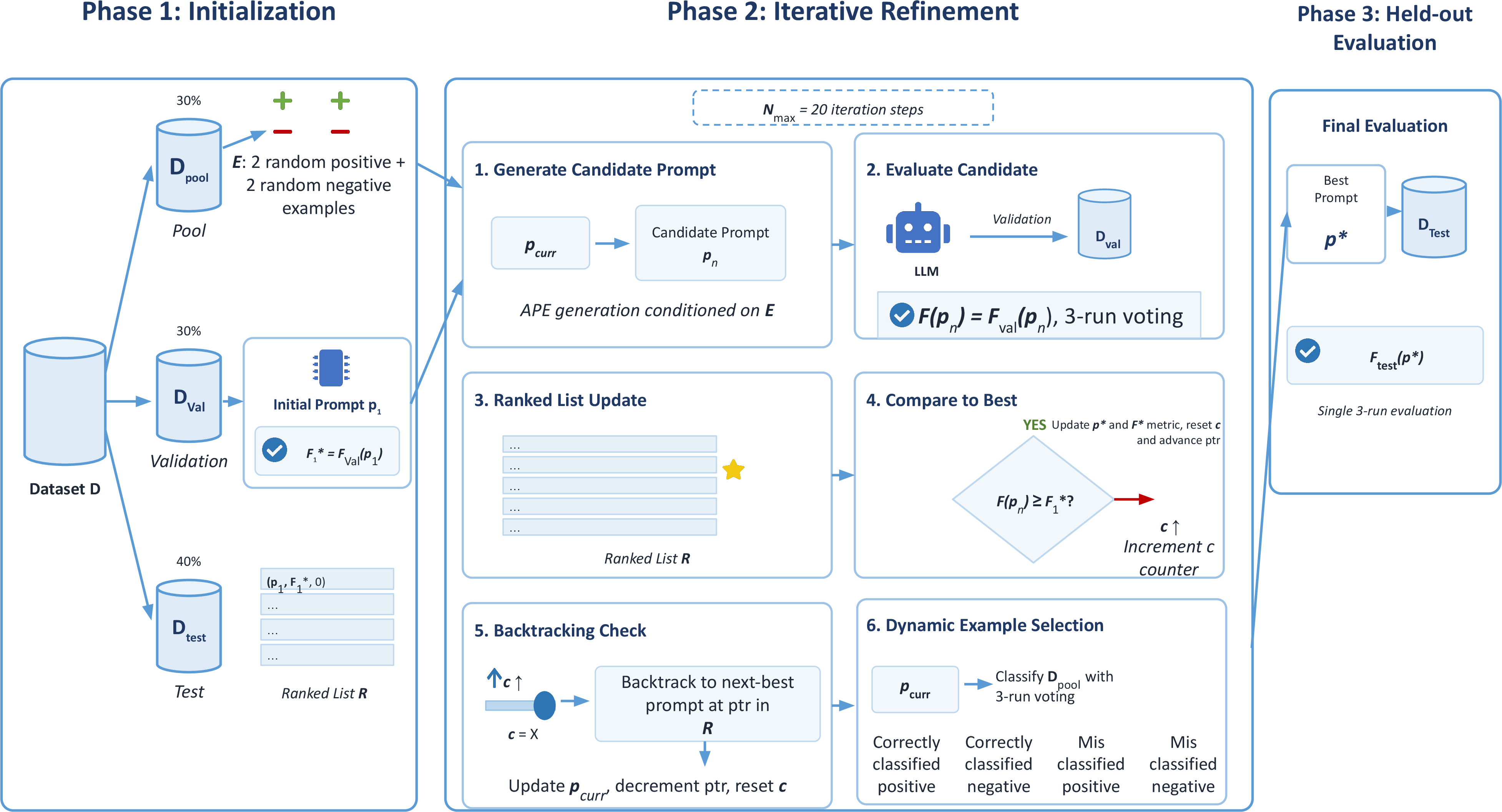
3.3 Algorithm and workflow↩︎
Figure 1 and Algorithm 2 present the same procedure as a diagram and as pseudocode, respectively. We describe the three phases below, with line numbers referring to Algorithm 2.
Phase 1: Initialisation (ll. 1–5). The dataset \(D\) is partitioned into \(D_{\text{pool}}\) (30%), \(D_{\text{val}}\) (30%), and \(D_{\text{test}}\) (40%); these proportions balance the competing demands of in-context learning, low-variance validation scoring, and a low-variance final test estimate (see Appendix 9). The example batch \(E\) is seeded with two random positive and two random negative examples from \(D_{\text{pool}}\). The initial prompt \(p_1\) is scored on \(D_{\text{val}}\) to obtain its weighted F1, which we denote \(F^{*}\) and use throughout the search as the best-so-far reference score against which subsequent candidates are compared. The triple \((p_1, F^{*}, 0)\) is then inserted into the ranked list \(\mathcal{R}\).
Phase 2: Iterative refinement (ll. 6–22). For up to \(N_{\max} = 20\) iterations, the procedure performs six steps:
Generate candidate (l. 8). A new prompt \(p_n\) is generated by the LLM, conditioned on the current prompt \(p_{\text{curr}}\) and the balanced example batch \(E\). Conditioning on \(E\) exposes the proposer to concrete instances of where the current prompt succeeds and fails, following the error-conditioned refinement principle introduced by ProTeGi [14] and PE2 [12].
Evaluate candidate (l. 10). \(p_n\) is scored on \(D_{\text{val}}\) using 3-run majority voting (Section 3.6). Voting reduces run-to-run variability at the cost of three inference passes per candidate; this matters because the backtracking trigger below depends on F1 comparisons across iterations, and evaluation noise would otherwise propagate directly into search dynamics.
Update ranked list (l. 12). The triple \((p_n, F(p_n), n)\) is inserted into \(\mathcal{R}\), kept sorted by F1. Maintaining the full ranked history (rather than only the current best) is what enables the bounded backtracking step below.
Compare to best (ll. 13–17). If \(F(p_n) \geq F^{*}\), the best prompt and reference score are updated, the failure counter \(c\) is reset, and the pointer \(ptr\) advances. Otherwise, \(c\) is incremented.
Backtracking check (ll. 18–21). If \(c\) reaches the patience threshold \(X = 3\), the search abandons the current trajectory and resumes from the next-best prompt in \(\mathcal{R}\) via the pointer \(ptr\). The threshold \(X\) is an interpretable exploration–exploitation knob: \(X = 1\) over-reacts to evaluation noise, while large values waste iterations on plateaus. We set \(X = 3\) based on the sensitivity analysis in Appendix 9.
Select examples for the next iteration (ll. 22–23). \(D_{\text{pool}}\) is re-classified with \(p_{\text{curr}}\), and \(E\) is refreshed with one correctly classified positive, one correctly classified negative, one misclassified positive, and one misclassified negative. This balanced four-tuple guarantees that the proposer simultaneously sees success and failure signals on both classes — a property that matters because the optimisation objective is F1 on a potentially imbalanced label distribution.
Phase 3: Held-out evaluation (l. 24). The best prompt \(p^{*}\) is scored once on \(D_{\text{test}}\) under the same 3-run majority-voting protocol. Because \(D_{\text{test}}\) is consulted only at this final step, the reported F1 is a genuine held-out estimate rather than a selection-inflated one.

3.4 BT-APE: Method Design and Inspirations↩︎
We propose BT-APE (Back-Tracking APE), a lightweight prompt optimisation procedure designed for settings where labelled data is scarce and each candidate evaluation is expensive. Given an initial prompt \(p_0\) and a small pool \(D_{\text{pool}}\) of labelled examples, BT-APE iteratively proposes new prompts conditioned on the model’s behaviour on a balanced batch of correct and incorrect predictions, and maintains a ranked history \(\mathcal{R}\) of all candidates evaluated so far. The full procedure is given in Algorithm 2 and summarised in Figure 1. In the following, we describe the main elements of the approach, and then we describe the figure and the algorithm in details. The approach consists of three defining components.
3.4.0.1 Explicit, bounded back-tracking.
BT-APE maintains a ranked list \(\mathcal{R}\) of all evaluated candidates sorted by F1, together with a pointer \(ptr\) that identifies the prompt currently being refined. The search remains on the current trajectory until \(X = 3\) consecutive iterations fail to improve over the best score \(F^{*}\), at which point \(ptr\) jumps to the next-best prompt in \(\mathcal{R}\). This yields an interpretable patience parameter and prevents the search from lingering in unproductive neighbourhoods of the prompt space.
3.4.0.2 Balanced, dynamic example selection.
At every iteration, after classifying \(D_{\text{pool}}\) with the current prompt \(p_{\text{curr}}\), BT-APE re-samples the example batch \(E\) to contain one correctly classified positive, one correctly classified negative, one misclassified positive, and one misclassified negative example. This guarantees that the proposer simultaneously sees success and failure signals on both classes—a property that matters because our optimisation objective is F1 on a potentially imbalanced label distribution.
3.4.0.3 Stable evaluation via majority voting.
Every candidate is evaluated on the held-out validation split using 3-run majority voting. Because the back-tracking trigger depends on F1 comparisons across iterations, evaluation noise directly affects search dynamics; majority voting reduces LLM stochasticity at the cost of three times the inference budget per candidate. We use a fixed 30/30/40 pool/val/test split throughout the search so that F1 values entered into \(\mathcal{R}\) are directly comparable across iterations.
3.4.1 Baseline and Positioning↩︎
To assess whether the simplicity of BT-APE comes at a cost, we compare it against PE2 [12] as a representative baseline. PE2 is a natural point of comparison: it shares the same single-trajectory, history-aware backbone, and formalises prompt optimisation as a sequence of meta-prompted proposals \[p^{(t+1)} = \mathcal{M}_{\text{proposal}}\bigl(p^{(t)}, B;\, p_{\text{meta}}\bigr), \label{eq:pe2-proposal}\tag{1}\] over a batch \(B = \{(x, y, y')\}\) of inputs, ground-truth labels, and current predictions, with a history of prior prompts from which back-tracking is possible by re-selecting the top-\(n\) candidates from \(P^{(0)} \cup P^{(1)} \cup \ldots \cup P^{(t)}\) at every step [12]. We exclude population-based evolutionary approaches such as EPiC [44] from this comparison: they are well suited to code generation, where auto-generated unit tests validated via AST parsing make the fitness oracle cheap and large populations can be evaluated in parallel at low cost—a setting that does not match our binary-classification task, where each candidate evaluation requires three full classification runs over \(D_{\text{val}}\).
BT-APE and PE2 differ along three axes that map onto the three components above, and each axis has a concrete resource-consumption consequence which we quantify empirically in Appendix 11.
First, PE2 re-selects the top-\(n\) prompts from the full history at every step, whereas BT-APE commits to the current trajectory and triggers an explicit jump only when a fixed patience threshold is exceeded. Conditioning each proposal on the top-\(n\) history means that PE2’s per-iteration input context grows roughly linearly with the iteration count, while BT-APE’s remains bounded. Empirically, at \(N_{\max} = 20\), PE2 consumes approximately \(72\%\) more cumulative input tokens than BT-APE across all 15 (dataset, LLM) configurations (paired Wilcoxon, \(p < 10^{-4}\), large effect size; see Table 14).
Second, PE2 conditions the proposer on an unconstrained error batch; BT-APE enforces a class- and outcome-balanced batch at every iteration. The use of failure examples to drive prompt edits is also central to ProTeGi [14], which conditions a “textual gradient” prompt on model errors and then applies a second prompt to edit \(p_0\) in the opposite semantic direction. BT-APE adopts this principle without the two-step gradient-then-edit decomposition, since a single proposal call conditioned on a balanced error batch is sufficient in our binary-classification setting and avoids doubling the LLM call cost per iteration.
Third, BT-APE relies on 3-run majority voting on a fixed validation split, ensuring directly comparable F1 values across iterations—a property that bandit-style subsampling, as used in ProTeGi’s selection step [14], would not preserve.
Taken together, these three design choices translate into a substantially lighter resource profile at equivalent accuracy: in addition to the input-token reduction noted above, BT-APE incurs approximately \(60\%\) lower mean proposer latency and \(66\%\) shorter total wall-clock time than PE2 across the full experimental grid (Appendix 11). On a cost-normalised basis, BT-APE delivers each percentage point of \(wF_1\) at roughly \(27\%\) of PE2’s input-token cost and \(34\%\) of its wall-clock cost. This is the main practical motivation for the design: it enables deployment on resource-constrained or air-gapped servers, which are typically preferred in RE settings where requirements confidentiality discourages reliance on hosted APIs.
The defaults \(X = 3\) and \(N_{\max} = 20\) are motivated by the sensitivity analysis in Appendix 9, which shows that \(X = 1\) yields unstable trajectories while \(X \in \{3, 5\}\) behave comparably on accuracy at increasing resource cost.
3.5 Prompt Structure and Class Definitions↩︎
A central component of the BT-APE classification prompt is the set of class definitions that instruct the LLM on how to distinguish between requirement categories. In the optimisation loop, the class definitions are the primary variable component of the prompt \(p\), while the surrounding scaffolding (output-format instructions, task framing) remains fixed.
We restrict optimisation to class definitions for two reasons. First, the output-format instructions are dictated by the evaluation pipeline: rewriting them risks producing responses the parser cannot decode, conflating prompt-quality variation with parsing failures. Second, prior work on prompt sensitivity in classification tasks [6], [30] identifies category descriptions as the primary lever through which prompts influence label decisions, while task framing contributes comparatively little once a minimally adequate version is in place. Confining the search to this component also keeps the prompt space small enough to be explored within the bounded iteration budget (\(N_{\max} = 20\)).
Two strategies are proposed for initializing these definitions, each serving as a different starting point \(p_1\) for the optimization process:
Simple Definitions (BT-APE-Uninformed). Class definitions are one-sentence intuitive descriptions written by Author 1 without consulting RE literature or standards, reflecting a minimal-effort starting point. Examples: “Functional: what the system should do.”; “Quality: how well the system should do it.”; “Security: protection against unauthorised access or harm.” The full set is given in Appendix 14.
Literature-Based Definitions (BT-APE-Informed). Class definitions are curated and synthesized from established software engineering literature by an RE expert (last author). The functional and non-functional requirement definitions are derived from Glinz’s [45] summary of the literature definitions, which characterizes functional requirements in terms of the essential functions a system must perform, the services it must offer, and the behaviours it must exhibit under specified conditions—focusing on the inputs (stimuli), outputs (responses), and the behavioural relationships between them. The quality requirement definitions are synthesized from quality-modeling literature and standards [46], [47], expressing how well a system or service should execute an intended function through product quality aspects (e.g., functional suitability, reliability, performance, efficiency, usability, maintainability, security, compatibility, portability) and quality in use aspects (e.g., satisfaction, effectiveness, freedom from risk, context coverage). The security requirement definitions are derived from the security requirements engineering literature and standards [48]–[50], characterizing security requirements as prescriptive constraints imposed on a system’s functional behaviour to operationalize its security goals—restricting how functions are performed to prevent, detect, or recover from harm, while specifying security policies and addressing risks, threats, and assets. The non-functional, non-quality, and non-security definitions are obtained by negating their functional, quality, and security counterparts, respectively. These definitions capture the nuanced distinctions recognized in the domain, such as differentiating sub-categories of quality requirements (e.g., performance, security, usability). By grounding the initial prompt in domain knowledge, the LLM is provided with richer semantic context from the outset.
In both cases, the definitions are subject to iterative refinement during the optimization process: at each iteration, the BT-APE mechanism may edit, expand, or restructure the class definitions based on misclassified and correctly classified examples from the training set \(D_{\text{pool}}\). The goal of introducing these different definitions is to check whether a more informed initialization—rooted in domain literature—leads to superior classification performance compared to uninformed starting point, and whether this advantage persists after multiple rounds of optimization. All the prompt structures and definitions are given in Appendix 14.
3.6 Inference-time voting protocol↩︎
The protocol described in this section is not specific to BT-APE; it is an evaluation safeguard applied uniformly to all prompting strategies (zero-shot, few-shot, CoT, CoT+few-shot, PE2, and BT-APE) whenever a prompt is scored on \(Dval\) or \(Dtest\), so that comparisons across strategies are made under identical conditions.
To mitigate the run-to-run variability of LLM outputs, we adopt a majority voting strategy during inference. Although we set the decoding temperature to \(0\), identical prompts can still yield different outputs across runs due to stochastic sampling at non-zero temperature settings, GPU non-determinism, and request batching at the inference backend [51]. For each classification instance, the model is therefore executed three times with the same prompt, and the final label is assigned by majority vote: the class predicted in at least two out of three runs is selected as the final output. This protocol applies uniformly to baseline strategies and to the in-loop validation scoring of BT-APE (Algorithm 2, line 10) and PE2 (Algorithm 4).
4 Research Design↩︎
4.1 Research Questions↩︎
The research design is guided by the following research questions (RQs):
RQ1: What is the performance of BT-APE in requirements classification compared to standard prompt engineering approaches?
This question aims to evaluate the overall effectiveness of BT-APE relative to standard prompt engineering methods in the context of requirements classification. To answer this question, 1) we assess BT-APE’s performance across different LLMs and datasets using descriptive statistics (e.g., mean, standard deviation) for key metrics such as weighted-F1 score in comparison to other baseline methods. 2) We then conduct statistical significance testing to compare BT-APE results against the results obtained by the baseline methods. This allows us to determine whether BT-APE offers a meaningful improvement over manual or fixed prompt designs.RQ2: What is the influence of the choice of dataset and LLM on the performance of BT-APE?
This question aims to statistically assess whether the selected datasets and LLMs have a significant impact on the performance of the BT-APE process. To answer it, we execute BT-APE across the three classification tasks using each of the five LLMs and collect the resulting weighted-F1 scores, yielding one value per (dataset, LLM) combination. We then apply distribution-free statistical tests to determine whether performance differences across datasets and across LLMs are statistically significant, and report a rank-based effect size to quantify the strength of each factor. This analysis enables us to assess the individual effects of datasets and LLMs on BT-APE effectiveness.RQ3: What are the defining characteristics of optimal prompts, and how do these emerge and evolve through BT-APE iterations?
This question identifies the characteristics of effective prompts by analysing how they evolve across BT-APE iterations. We extract lexical (sentence count, word count, lexical diversity), syntactic (verb count, syntactic complexity), and semantic features (ambiguity score, semantic drift) from every prompt generated during the BT-APE process, and log them together with the validation weighted-F1 score of the prompt that produced them.Because each prompt is conditioned on its predecessor, observations within a (dataset, LLM) trajectory are not independent. We therefore analyse the data with a linear mixed-effects model (LMM) — prompt features as fixed effects, a random intercept per trajectory — so that coefficients estimate the within-trajectory association between each feature and performance, separated from between-configuration variance. Full model specification, robustness checks, hypotheses, and effect-size reporting are given in the statistical test design.
One interpretive caveat is integral to the research question rather than to the test design: semantic drift (\(SD\)) is by construction a property of consecutive prompts, not of a prompt in isolation. A positive coefficient on \(SD\) would characterise successful search dynamics, not actionable guidance for designing a static prompt. We therefore separate state features (length, verb count, punctuation, lexical diversity, syntactic complexity, ambiguity) from the transition feature (\(SD\)), and restrict design claims to the former.
RQ4: To what extent does BT-APE-Informed influence classification performance compared to i) BT-APE-Uninformed and ii) how do both approaches perform relative to their respective best baseline models?
This question examines the effect of class definition quality on the BT-APE process by comparing two variants: BT-APE-Uninformed and BT-APE-Informed. To answer this, both variants are evaluated across the same datasets and LLMs under identical experimental conditions. Their performance is compared using key metrics such as Weighted \(F1\) score with statistical significance testing applied to assess whether BT-APE-Informed yields a meaningful improvement over BT-APE-Uninformed. In addition, each variant is compared against its respective best-performing baseline to determine how much improvement is achieved relative to standard prompt engineering approaches. This helps disentangle whether gains are driven primarily by the quality of the initial class definitions or by the iterative optimization process itself. Overall, this analysis isolates the role of class definitions as a design variable and evaluates whether domain-informed definitions provide a consistent advantage, or whether iterative optimization can compensate for simpler starting points.
4.2 Shared Experimental Settings↩︎
Tasks & Datasets. We evaluate BT-APE on three requirements classification tasks, each representing a distinct and well-studied problem in requirements engineering:
Functional-Quality classification based on the PROMISE Refined: In this task, we consider four binary classification tasks: Functional, Only Functional, Quality, and Only Quality. Specifically, this means that each data point should be evaluated solely on whether it meets functional requirements, quality requirements, or both. For every data point, we treat Functional and Quality as two separate ground-truth labels. The Only Functional task is then defined as instances that are labeled as Functional but not Quality, while the Only Quality task covers instances labeled as Quality but not Functional.
Functional–Non-Functional Binary Classification: Distinguishing between functional and Not-Functional requirements. This task addresses the fundamental separation between what a system should do and how well it should perform.
Security Binary Classification: Determining whether a requirement is security-related or not. This task targets a single quality concern and is particularly relevant for safety- and security-critical systems.
We selected three well-established requirements datasets to represent the above tasks. These datasets have been extensively utilized in prior research involving machine learning and language models for RE, such as in [20], [21], [23], [25], [26]. A summary is presented in Table ¿tbl:tab:datasets?.
column2 = c, cell11 = c, hline1,5 = -0.08em, hline2 = -0.05em, Dataset &
# Reqs. & Main Classes & Sources
PROMISE (NFR) & 625 & 255 Functional Requirements (FR),
370 Non-Functional Requirements (NFR). & Developed by Cleland-Huang et al.;
used by Kurtanović and Maalej,
Hey et al., and Alhoshan et al.
PROMISE (Refined) & 625 & 310 Functional (FR), 230 is-only Functional (FR_only).
382 Quality (QA), 302 is-only Quality (Q_only) & Developed by Dalpiaz et al.;
includes reclassification of PROMISE;
used by Hey et al. and Alhoshan et al.
SecReq & 510 & 187 Security-related (Sec), 323 Non-security (NSec) & Developed by Knauss et al.;
based on ePurse, CPN, and GPS;
used by Varenov et al. and Kobilica et al.
PROMISE NFR Dataset: Developed by Cleland-Huang et al. [19], [52], this dataset comprises 625 requirements, including 255 FRs and 370 NFRs. This dataset has been widely adopted in the literature, including by Kurtanović and Maalej [23], Hey et al. [25], and Alhoshan et al. [26].
PROMISE Refined Dataset: Introduced by Dalpiaz et al. [20], this dataset re-annotates the PROMISE NFR dataset. For binary classification, requirements are labeled as Quality (382) vs. non-Quality (243), and (302) labeled as quality only; and Functional (310) vs. non-Functional (315), and (230) labeled as functional only requirements. This dataset has been employed in studies such as [25], [26].
SecReq Dataset: Created by Knauss et al. [21], [53], the SecReq dataset contains 510 requirements, split into 187 security-related and 323 non-security-related instances. The data were collected from three projects: Common Electronic Purse (ePurse), Customer Premises Network (CPN), and Global Platform Specification (GPS). It has been utilized in multiple studies, including [54], [55].
LLMs Selection. To select a representative set of instruction-tuned LLMs with approximately 7–8 billion parameters, we consulted the Hugging Face Open LLM Leaderboard1 as a reference for identifying widely used open-source models. The selection was guided by model availability, parameter scale, organisational diversity, and architectural characteristics rather than reported benchmark performance. Our goal is not to identify the single best-performing model on requirements classification, but to test whether BT-APE generalises across architectures and whether it consistently beats classical prompting baselines; using models that span different organisations, attention mechanisms, and pretraining corpora gives us a more honest stress test of generalisation than concentrating on top-ranked models from a single family. The 7–8B parameter range is chosen because models of this size can be hosted locally on a single commodity GPU, which reflects the practical RE setting where requirements confidentiality discourages reliance on hosted proprietary APIs [2]. Based on these criteria, we selected five models developed by different research organizations:
| Model | Parameters | Attention Mechanism | Pretraining/Instruction Tasks | Organization |
|---|---|---|---|---|
| Qwen2 | 7B | RoPE, MQA | Multilingual corpora, code, instruction tuning | Alibaba Cloud |
| Falcon3 | 7B | MQA | English web text, instruction data | TII (UAE) |
| Granite-3.2 | 8B | Scaled-dot attention (factual) | Business text, code, domain adaptation | IBM Research |
| Ministral | 8B | Sliding Window Attention | Instruction datasets, reasoning tasks | Mistral AI |
| LLaMA-3 | 8B | GQA, RoPE | Multilingual corpora, SFT tasks | Meta AI |
Qwen2-7B-Instruct (Alibaba Cloud): employs Rotary Positional Embeddings combined with Multi-Query Attention to support efficient attention computation. It is pretrained on multilingual corpora and programming code and further refined using human-aligned instruction datasets.
Falcon3-7B-Instruct (Technology Innovation Institute): uses Multi-Query Attention to reduce inference-time memory requirements. Its training data primarily consists of large-scale English web text and curated instruction-following datasets.
Granite-3.2-8B-Instruct (IBM Research): applies optimized scaled dot-product attention with a focus on factual grounding. It is trained on business-oriented text, programming code, and domain-specific adaptation tasks.
Ministral-8B-Instruct-2410 (Mistral AI): incorporates Sliding Window Attention to limit attention to local contexts and improve computational efficiency. It is trained on instruction-following datasets and reasoning-oriented benchmarks.
Meta-Llama-3-8B-Instruct (Meta AI): adopts Grouped-Query Attention together with Rotary Positional Embeddings to balance efficiency and representational capacity. Its pretraining relies on large-scale multilingual corpora and supervised fine-tuning on human-aligned datasets.
Table 1 summarizes the main technical characteristics of the selected models, including parameter size, attention mechanisms, pretraining and instruction tasks, and organizational origin. These descriptions provide contextual background for the experimental setup without presupposing differences in task performance.
Evaluation Metrics. We used four standard evaluation metrics: Precision (\(P\)), Recall (\(R\)), Weighted F1 Score (\(wF_1\)). These metrics are well-suited for imbalanced classification tasks and allow us to evaluate both general accuracy and recall-oriented performance.
Precision (\(P\)): The proportion of correctly predicted instances for a given class among all instances predicted as belonging to that class. \[P = \frac{TP}{TP + FP}\]
Recall (\(R\)): The proportion of correctly predicted instances for a given class among all actual instances of that class. \[R = \frac{TP}{TP + FN}\]
Weighted F1 Score (\(wF_1\)): The harmonic mean of precision and recall, computed for each class and averaged using the number of true instances (support) as weights. \[wF_1 = \sum_{c \in C} w_c \cdot \frac{2 \cdot P_c \cdot R_c}{P_c + R_c}\]
ìIn the above equations, \(TP\), \(FP\), and \(FN\) denote true positives, false positives, and false negatives, respectively; \(w_c\) represents the support (i.e., the proportion of instances) for class \(c\), and \(C\) is the set of all target classes.
4.3 Prompt Baselines Selection↩︎
We compare our approach against five widely adopted prompting strategies that together cover the standard spectrum of techniques used to elicit classification performance from LLMs without task-specific fine-tuning: four in-context learning baselines of increasing sophistication, and one APE baseline. These baselines are selected because they are (i) model-agnostic and reproducible across both large and small language models, (ii) computationally lightweight and therefore compatible with our SLM deployment setting, and (iii) established as canonical reference points in recent RE and NLP classification studies [6]. The five baselines are:
Zero-shot prompting: The model receives only a task description and label definitions, with no labeled examples. This baseline measures the model’s ability to perform the classification task purely from its pretrained knowledge and the natural-language specification of the task.
Few-shot prompting: The model is provided with a small set of labeled input–output examples alongside the task description. This baseline isolates the contribution of demonstration-based in-context learning, allowing us to measure how much performance improves when the model is exposed to representative instances of each requirement category.
Chain-of-Thought (CoT) prompting: The model is explicitly instructed to generate intermediate reasoning steps before producing the final output. This baseline tests whether eliciting structured reasoning improves classification on requirements that demand multi-step interpretation, such as distinguishing functional from non-functional aspects in compound statements.
CoT with Few-shot prompting: The model receives multiple labeled examples, each accompanied by an explicit reasoning trace and the final label. This baseline combines demonstration-based learning with reasoning elicitation and represents the strongest non-optimised prompting configuration commonly reported in the literature.
PE2 (APE) [12]: The prompt is iteratively refined by a meta-prompted LLM conditioned on the top-\(n\) historical prompts with their validation weighted-F1 scores and a batch of misclassifications observed on a held-out pool. Unlike the four baselines above, which keep the prompt fixed, PE2 actively searches the prompt space using the same iteration budget and evaluation protocol as our method. This baseline is the most directly comparable reference point for our approach, since both methods are single-trajectory, history-aware APE procedures driven by errors on a held-out set; its inclusion is what allows us to attribute any performance gap to our three algorithmic contributions—bounded back-tracking, balanced four-tuple example selection, and majority-voted F1—rather than to the use of prompt optimisation in general. Full algorithmic and implementation details, together with a precise enumeration of the differences from our method, are given in Appendix 10 (Algorithm 4).
The exact prompt templates used for each baseline are provided in the replication package [22].
4.4 Experimental Design for RQ1↩︎
Statistical Significance.2 To assess whether the performance differences between each baseline prompting strategy and the proposed BT-APE approach are statistically significant, we analyse the per-cell differences in \(wF_1\) (i.e., \(\Delta = wF_{1,\text{BT-APE}} - wF_{1,\text{Baseline}}\)). All differences across datasets and LLMs are pooled for each baseline strategy.
We then conduct a non-parametric Wilcoxon signed-rank test to evaluate whether BT-APE achieves a higher mean \(wF_1\) than the baseline. All tests are performed at a significance level of \(\alpha = 0.05\), with \(p\)-values adjusted using the Holm–Bonferroni procedure to account for multiple baseline comparisons.
For each comparison between BT-APE and a baseline strategy, the following hypotheses are defined:
\(H^{\text{RQ}1}_{1,0}\): The mean difference in performance (\(wF_1\)) between BT-APE and the baseline strategy is zero (\(\Delta = 0\)).
\(H^{\text{RQ}1}_{1,A}\): BT-APE achieves a higher mean performance (\(wF_1\)) than the baseline strategy (\(\Delta > 0\)).
Effect Size and Interpretation. We report the mean difference in \(wF_1\) (\(\Delta\)) with 95% confidence intervals. This statistic is centred at zero when there is no improvement:
\(\Delta = 0\) indicates no systematic difference.
Positive values indicate that BT-APE outperforms the baseline.
Negative values indicate that the baseline outperforms BT-APE.
Effect size \(r\) is computed as \(r = Z / \sqrt{N}\), where \(Z\) is the standardised Wilcoxon test statistic and \(N\) is the number of observations. Magnitudes are interpreted as: negligible (\(r < 0.10\)), small (\(0.10 \leq r < 0.30\)), moderate (\(0.30 \leq r < 0.50\)), and large (\(r \geq 0.50\)) [56].
4.5 Experimental Design for RQ2↩︎
Factors Analysis. To address RQ2, we investigate how the performance of BT-APE varies as a function of two independent variables—Datasets/Tasks and LLMs—as well as their interaction. The final BT-APE results consist of one \(wF_1\) value per (Dataset, LLM) combination, yielding a \(3 \times 5\) design with \(n = 15\) observations.
Datasets/Tasks. We test whether performance (\(wF_1\)) differs significantly across requirements classification tasks (Security, Functional, and Quality).
LLMs. We test whether performance (\(wF_1\)) differs significantly across the selected LLMs.
Statistical Significance. We first assess the normality assumption with the Shapiro–Wilk test. Given the small sample and borderline normality, we adopt distribution-free Friedman tests for the two main effects rather than relying on the assumptions of parametric ANOVA. We test the dataset effect using LLMs as blocks, and the LLM effect using datasets as blocks. All tests are conducted at a significance level of \(\alpha = 0.05\). The following hypotheses are defined:
Dataset/Task effect.
\(H^{\text{RQ}2}_{1,0}\): There is no statistically significant difference in \(wF_1\) across datasets.
\(H^{\text{RQ}2}_{1,A}\): There is a statistically significant difference in \(wF_1\) across datasets.
LLM effect.
\(H^{\text{RQ}2}_{2,0}\): There is no statistically significant difference in \(wF_1\) across LLMs.
\(H^{\text{RQ}2}_{2,A}\): There is a statistically significant difference in \(wF_1\) across LLMs.
Effect Size and Interpretation. We report Kendall’s \(W\) as the effect size for each Friedman test, which ranges from 0 (no agreement among blocks) to 1 (perfect agreement). Larger values indicate a stronger and more consistent factor effect across the blocking variable. As the interaction is not estimable under a single-replicate design, we do not test it formally; where the cell-level results suggest task-dependent model behaviour, we describe it descriptively.
4.6 Experimental Design for RQ3↩︎
Prompt Feature Extraction. We extract and log a set of lexical, syntactic, and semantic features from each prompt generated during BT-APE iterations. These features are defined and computed as follows.
a) Lexical Features.
Sentence Count (\(SC\)): The number of sentences in the prompt, measured using sentence segmentation. \[SC = \text{Number of sentences in } P\]
Word Count (\(WC\)): The total number of words or tokens in the prompt. \[WC = \sum_{i=1}^{n} \delta(w_i), \quad \delta(w_i) = \begin{cases} 1, & \text{if } w_i \text{ is a word} \\ 0, & \text{otherwise} \end{cases}\]
Punctuation/Markers Count (\(PM\)): The number of structural markers such as colons, dashes, or line breaks. \[PM = \sum_{c \in P} \delta(c), \quad \delta(c) = \begin{cases} 1, & \text{if } c \in \{\texttt{:}, \texttt{-}, \texttt{.}, \texttt{\textbackslash n}, \ldots\} \\ 0, & \text{otherwise} \end{cases}\]
Lexical Diversity (\(LD\)): The ratio of unique words to total words, indicating vocabulary richness. \[LD = \frac{|\text{Unique}(w_1, w_2, \ldots, w_n)|}{WC}\]
b) Syntactic Features.
Verb Count (\(VB\)): The number of verbs in the prompt, identified via part-of-speech tagging. \[VB = \sum_{i=1}^{n} \delta(\text{POS}(w_i) = \text{VERB})\]
Syntactic Complexity (\(SCx\)): The average depth of the dependency parse tree over all tokens in the prompt. \[SCx = \frac{1}{n} \sum_{i=1}^{n} \text{depth}(w_i)\] where \(\text{depth}(w_i)\) denotes the number of dependency links from word \(w_i\) to the root.
c) Semantic Features.
Ambiguity Score (\(AS\)): quantifies the vagueness of a prompt based on the presence of ambiguous or underspecified terms, commonly referred to as “smelly” words (e.g., some, many, etc., maybe, often, unclear, various). The score is computed heuristically as: \[AS = \frac{1}{WC} \sum_{i=1}^{WC} \delta(w_i \in D_{\text{amb}})\] where:
\(WC\) is the total word count of the prompt,
\(w_i\) is the \(i^{\text{th}}\) word in the prompt,
\(D_{\text{amb}}\) is a predefined dictionary of ambiguity-inducing terms,
\(\delta(\cdot)\) is an indicator function that returns 1 if \(w_i \in D_{\text{amb}}\), and 0 otherwise.
Semantic Drift (\(SD\)): quantifies the semantic change between the current prompt and the immediately preceding one, computed as the cosine distance between their embedding vectors. For a sequence of \(n\) prompts, the drift at iteration \(i\) is defined as: \[SD_i = \begin{cases} 0, & \text{if } i = 1 \\ 1 - \dfrac{\vec{e}_{i} \cdot \vec{e}_{i-1}}{\|\vec{e}_{i}\| \|\vec{e}_{i-1}\|}, & \text{if } i > 1 \end{cases}\] where \(\vec{e}_i\) and \(\vec{e}_{i-1}\) are the embedding vectors of the prompts at iterations \(i\) and \(i-1\), respectively. This formulation captures the magnitude of semantic shift introduced at each step in the BT-APE process.
All of these features (lexical, syntactic, and semantic) are tracked across all BT-APE iterations to study how prompt structure changes over time and how such changes correlate with model performance improvements. We further distinguish between state features, which describe a prompt in isolation (\(SC\), \(WC\), \(PM\), \(LD\), \(VB\), \(SCx\), \(AS\)), and transition features, which describe a change between consecutive prompts (\(SD\)). This distinction matters for interpretation: a within-trajectory association between a state feature and performance can plausibly motivate prompt-design guidance, whereas an association involving \(SD\) characterises the dynamics of successful search rather than properties of a static prompt.
Statistical Model. The prompts generated across BT-APE iterations are not independent observations. Within a single (dataset, LLM) trajectory, every prompt is conditioned on its predecessor, shares the same proposer, and inherits the same starting point; across trajectories, baseline performance differs systematically with task difficulty and model capability (as established in RQ2). Pooling all prompts into an ordinary least-squares regression with \(wF_1\) as the response would therefore conflate within-trajectory variance—how performance changes as a single search evolves—with between-configuration variance, and would overstate the precision of the resulting coefficients by treating non-independent observations as independent.
To respect this nested structure, we estimate a linear mixed-effects model (LMM) in which prompt features enter as fixed effects and a random intercept is fitted for each (dataset, LLM) trajectory: \[wF_{1,ij} \;=\; \beta_0 + \sum_{k} \beta_k\, x_{k,ij} \;+\; u_j \;+\; \varepsilon_{ij}, \qquad u_j \sim \mathcal{N}(0,\sigma_u^2),\; \varepsilon_{ij} \sim \mathcal{N}(0,\sigma_\varepsilon^2),\] where \(i\) indexes the iteration within trajectory \(j \in \{1, \ldots, 15\}\), \(x_{k,ij}\) is the value of the \(k\)-th prompt feature at iteration \(i\) of trajectory \(j\), \(u_j\) is the random intercept absorbing configuration-level differences in baseline \(wF_1\), and \(\varepsilon_{ij}\) is the residual. The fixed-effect coefficients \(\beta_k\) therefore estimate the within-trajectory association between each prompt feature and performance, after removing the contribution of the underlying (dataset, LLM) configuration. The model is estimated by restricted maximum likelihood (REML), and all features are standardised to zero mean and unit variance prior to fitting so that coefficient magnitudes are directly comparable.
Robustness Check on Terminal Prompts. As a complementary analysis that is independent of trajectory dynamics by construction, we also fit an ordinary least-squares regression on the terminal prompts \(p^{*}\) of each of the 15 trajectories (\(n = 15\)). The transition feature \(SD\) is excluded from this analysis as it is not defined for a single prompt. This terminal-prompt regression has limited statistical power but provides a sanity check: a feature whose within-trajectory effect under the LMM is contradicted by its sign on terminal prompts is unlikely to constitute reliable design guidance. We therefore report a feature as a robust correlate of effective prompts only when its LMM coefficient is statistically significant and its sign agrees with the terminal-prompt regression.
Hypotheses. All tests are conducted at a significance level of \(\alpha = 0.05\), with Holm–Bonferroni correction applied across the feature set to control the family-wise error rate.
\(H^{\text{RQ}3}_{1,0}\): After accounting for between-trajectory variance, prompt features have no statistically significant within-trajectory effect on \(wF_1\) (\(\beta_k = 0\) for all \(k\)).
\(H^{\text{RQ}3}_{1,A}\): At least one prompt feature has a statistically significant within-trajectory effect on \(wF_1\).
Effect Size and Interpretation. We report standardised fixed-effect coefficients \(\hat{\beta}_k\) with 95% confidence intervals for each feature. Positive coefficients indicate that, within a trajectory, an increase in the feature is associated with higher \(wF_1\); negative coefficients indicate the converse. The absolute magnitude of \(\hat{\beta}_k\) reflects the relative strength of the feature’s within-trajectory contribution.
At the model level, we report three quantities. The marginal \(R^2_m\) measures the proportion of variance in \(wF_1\) explained by the fixed effects alone, and is the appropriate analogue of the OLS \(R^2\) for the prompt-feature claim. The conditional \(R^2_c\) measures the proportion explained by fixed and random effects jointly, and indicates the total fit of the model. The intra-class correlation coefficient (ICC), \[\text{ICC} \;=\; \frac{\sigma_u^2}{\sigma_u^2 + \sigma_\varepsilon^2},\] quantifies the share of residual variance attributable to between-configuration differences rather than to within-trajectory prompt characteristics; a high ICC would indicate that most of the variation in \(wF_1\) is configuration-driven and that within-trajectory feature effects, however statistically significant, account for a comparatively small share of overall performance variation. Together, \(R^2_m\), \(R^2_c\), and the ICC provide a more honest accounting of where the explanatory power of the model lies than a single pooled \(R^2\) would.
As noted above, we treat \(SD\) separately in the interpretation: a significant within-trajectory coefficient on \(SD\) is described as a property of successful optimisation trajectories rather than as actionable guidance for designing a static prompt. Actionable design claims are restricted to state features whose coefficients are stable across the LMM and the terminal-prompt regression.
4.7 Experimental Design for RQ4↩︎
Class Definitions. As introduced in Section 3.5, we define two initialisation strategies for the prompt optimisation process. In BT-APE-Informed, the initial prompt is seeded with fine-grained class definitions curated from requirements engineering literature and standards. In BT-APE-Uninformed, no predefined class definitions are provided; instead, the algorithm begins with simple, minimal descriptions and iteratively refines them throughout the optimisation process. This design allows us to assess two complementary aspects: (1) whether domain-grounded definitions offer a measurable advantage as a starting point, and (2) whether the iterative optimisation is capable of discovering effective definitions independently, without relying on prior domain knowledge.
Statistical Significance. To assess whether the performance differences between BT-APE-Uninformed and BT-APE-Informed are statistically significant, we analyse two complementary dimensions.
Dimension 1: Final Performance Comparison. We analyse the per-cell differences in final optimised \(wF_1\) (i.e., \(\Delta_{\text{final}} = wF_{1,\text{BT-APE-Informed}} - wF_{1,\text{BT-APE-Uninformed}}\)). All differences across datasets and LLMs are pooled. We then conduct a Wilcoxon signed-rank test to evaluate whether BT-APE-Informed achieves a higher mean final \(wF_1\) than BT-APE-Uninformed. The test is performed at a significance level of \(\alpha = 0.05\). For this comparison, the following hypotheses are defined:
\(H^{\text{RQ}4}_{1,0}\): The mean difference in final performance (\(wF_1\)) between BT-APE-Informed and BT-APE-Uninformed is zero (\(\Delta_{\text{final}} = 0\)).
\(H^{\text{RQ}4}_{1,A}\): BT-APE-Informed achieves a higher mean final performance (\(wF_1\)) than BT-APE-Uninformed (\(\Delta_{\text{final}} > 0\)).
Dimension 2: Improvement-over-Baseline Comparison. Since each variant has its own independent baseline (fine-grained class definitions for BT-APE-Informed vs.minimal descriptions for BT-APE-Uninformed), we compute the per-cell gain for each variant relative to its own starting point: \[\Delta_{\text{Informed}} = wF_{1,\text{Informed-Opt}} - wF_{1,\text{Informed-Baseline}}\] \[\Delta_{\text{Uninformed}} = wF_{1,\text{Uninformed-Opt}} - wF_{1,\text{Uninformed-Baseline}}\] We then calculate the difference in gains: \[\delta_{\text{gain}} = \Delta_{\text{Informed}} - \Delta_{\text{Uninformed}}\] A separate Wilcoxon signed-rank test is applied to \(\delta_{\text{gain}}\) across all (dataset, LLM) pairs to evaluate whether the two variants improve equally over their respective baselines. The hypotheses for this dimension are:
\(H^{\text{RQ}4}_{2,0}\): The mean difference in gains (\(\delta_{\text{gain}}\)) between BT-APE-Informed and BT-APE-Uninformed is zero, i.e., both variants improve equally over their own baselines.
\(H^{\text{RQ}4}_{2,A}\): The mean difference in gains (\(\delta_{\text{gain}}\)) is not zero, i.e., one variant achieves greater relative improvement from its baseline than the other.
Effect Size and Interpretation. For both dimensions, we report the mean difference (\(\Delta_{\text{final}}\) and \(\delta_{\text{gain}}\) respectively) with 95% confidence intervals, following the same interpretation benchmarks defined in RQ1. This dual analysis allows us to isolate the contribution of class definitions as a design variable and assess: (a) whether domain-grounded definitions provide a lasting advantage in final performance, and (b) whether the iterative optimisation compensates for simpler starting points by achieving comparable or greater relative improvement from a lower baseline.
5 Experimental Results↩︎
In this section, we present the results of the classification experiments conducted on three datasets: Refined Promise, Promise NFR, and SecReq. Performance is reported using weighted F1 (\(wF_1\)) score for the overall (average) results, and per-class F1 score for the class-specific breakdowns.
Refined Promise Dataset Results
Table 2 presents the classification results for the Refined Promise dataset, which includes classes for Functional (F), Quality (Q), Only Functional (onlyF), and Only Quality (onlyQ).
| Model | Strategy | Average | F | Q | onlyF | onlyQ |
| wF1 | wF1 | wF1 | wF1 | wF1 | ||
| Qwen/Qwen2-7B-Instruct | Zero-shot | 0.413 | 0.421 | 0.594 | 0.421 | 0.215 |
| Few-shot | 0.500 | 0.390 | 0.615 | 0.640 | 0.356 | |
| CoT | 0.487 | 0.410 | 0.643 | 0.640 | 0.256 | |
| CoT + Few-shot | 0.547 | 0.537 | 0.636 | 0.640 | 0.374 | |
| APE-PE2 | 0.587 | 0.583 | 0.679 | 0.691 | 0.444 | |
| BT-APE | 0.595 | 0.579 | 0.685 | 0.679 | 0.437 | |
| Falcon3-7B-Instruct | Zero-shot | 0.125 | 0.082 | 0.185 | 0.082 | 0.152 |
| Few-shot | 0.559 | 0.677 | 0.544 | 0.677 | 0.337 | |
| CoT | 0.260 | 0.622 | 0.082 | 0.185 | 0.151 | |
| CoT + Few-shot | 0.635 | 0.729 | 0.672 | 0.729 | 0.409 | |
| APE-PE2 | 0.620 | 0.645 | 0.670 | 0.658 | 0.437 | |
| BT-APE | 0.607 | 0.656 | 0.662 | 0.663 | 0.446 | |
| Granite-3.2-8B-Instruct | Zero-shot | 0.463 | 0.557 | 0.256 | 0.557 | 0.483 |
| Few-shot | 0.515 | 0.672 | 0.260 | 0.672 | 0.455 | |
| CoT | 0.441 | 0.572 | 0.144 | 0.572 | 0.477 | |
| CoT + Few-shot | 0.476 | 0.649 | 0.557 | 0.215 | 0.483 | |
| APE-PE2 | 0.472 | 0.536 | 0.325 | 0.678 | 0.381 | |
| BT-APE | 0.477 | 0.529 | 0.337 | 0.667 | 0.373 | |
| Ministral-8B-Instruct-2410 | Zero-shot | 0.455 | 0.569 | 0.195 | 0.569 | 0.488 |
| Few-shot | 0.594 | 0.682 | 0.458 | 0.682 | 0.554 | |
| CoT | 0.362 | 0.481 | 0.051 | 0.481 | 0.436 | |
| CoT + Few-shot | 0.446 | 0.616 | 0.296 | 0.692 | 0.181 | |
| APE-PE2 | 0.646 | 0.642 | 0.672 | 0.647 | 0.590 | |
| BT-APE | 0.637 | 0.655 | 0.676 | 0.633 | 0.585 | |
| Llama-3-8B-Instruct | Zero-shot | 0.212 | 0.297 | 0.075 | 0.297 | 0.181 |
| Few-shot | 0.266 | 0.153 | 0.573 | 0.234 | 0.104 | |
| CoT | 0.283 | 0.274 | 0.473 | 0.274 | 0.112 | |
| CoT + Few-shot | 0.393 | 0.616 | 0.296 | 0.535 | 0.123 | |
| APE-PE2 | 0.540 | 0.683 | 0.305 | 0.625 | 0.571 | |
| BT-APE | 0.551 | 0.691 | 0.299 | 0.629 | 0.585 |
| Model | Strategy | Average | F | NFR |
| wF1 | wF1 | wF1 | ||
| Qwen/Qwen2-7B-Instruct | Zero-shot | 0.749 | 0.750 | 0.748 |
| Few-shot | 0.726 | 0.730 | 0.722 | |
| CoT | 0.668 | 0.609 | 0.727 | |
| CoT + Few-shot | 0.749 | 0.750 | 0.748 | |
| APE-PE2 | 0.838 | 0.858 | 0.833 | |
| BT-APE | 0.847 | 0.847 | 0.846 | |
| Falcon3-7B-Instruct | Zero-shot | 0.642 | 0.574 | 0.711 |
| Few-shot | 0.708 | 0.706 | 0.710 | |
| CoT | 0.753 | 0.751 | 0.755 | |
| CoT + Few-shot | 0.754 | 0.752 | 0.755 | |
| APE-PE2 | 0.843 | 0.814 | 0.838 | |
| BT-APE | 0.831 | 0.828 | 0.833 | |
| Granite-3.2-8B-Instruct | Zero-shot | 0.703 | 0.711 | 0.695 |
| Few-shot | 0.720 | 0.705 | 0.736 | |
| CoT | 0.708 | 0.701 | 0.714 | |
| CoT + Few-shot | 0.774 | 0.754 | 0.794 | |
| APE-PE2 | 0.816 | 0.819 | 0.833 | |
| BT-APE | 0.820 | 0.812 | 0.827 | |
| Ministral-8B-Instruct-2410 | Zero-shot | 0.377 | 0.094 | 0.659 |
| Few-shot | 0.722 | 0.721 | 0.723 | |
| CoT | 0.722 | 0.721 | 0.722 | |
| CoT + Few-shot | 0.722 | 0.727 | 0.716 | |
| APE-PE2 | 0.853 | 0.838 | 0.834 | |
| BT-APE | 0.847 | 0.846 | 0.848 | |
| Llama-3-8B-Instruct | Zero-shot | 0.716 | 0.723 | 0.710 |
| Few-shot | 0.680 | 0.695 | 0.665 | |
| CoT | 0.679 | 0.699 | 0.659 | |
| CoT + Few-shot | 0.717 | 0.723 | 0.711 | |
| APE-PE2 | 0.780 | 0.791 | 0.814 | |
| BT-APE | 0.792 | 0.778 | 0.805 |
| Model | Strategy | Average | Security | Non-Security |
| wF1 | wF1 | wF1 | ||
| Qwen/Qwen2-7B-Instruct | Zero-shot | 0.651 | 0.468 | 0.835 |
| Few-shot | 0.818 | 0.736 | 0.900 | |
| CoT | 0.843 | 0.778 | 0.908 | |
| CoT + Few-shot | 0.843 | 0.778 | 0.908 | |
| APE-PE2 | 0.937 | 0.919 | 0.975 | |
| BT-APE | 0.945 | 0.908 | 0.981 | |
| Falcon3-7B-Instruct | Zero-shot | 0.848 | 0.789 | 0.907 |
| Few-shot | 0.836 | 0.774 | 0.897 | |
| CoT | 0.825 | 0.750 | 0.899 | |
| CoT + Few-shot | 0.848 | 0.789 | 0.907 | |
| APE-PE2 | 0.952 | 0.896 | 0.983 | |
| BT-APE | 0.947 | 0.903 | 0.991 | |
| Granite-3.2-8B-Instruct | Zero-shot | 0.819 | 0.789 | 0.849 |
| Few-shot | 0.766 | 0.672 | 0.861 | |
| CoT | 0.871 | 0.825 | 0.916 | |
| CoT + Few-shot | 0.836 | 0.774 | 0.897 | |
| APE-PE2 | 0.848 | 0.797 | 0.941 | |
| BT-APE | 0.859 | 0.783 | 0.934 | |
| Ministral-8B-Instruct-2410 | Zero-shot | 0.814 | 0.738 | 0.889 |
| Few-shot | 0.814 | 0.738 | 0.889 | |
| CoT | 0.787 | 0.745 | 0.829 | |
| CoT + Few-shot | 0.797 | 0.715 | 0.880 | |
| APE-PE2 | 0.935 | 0.863 | 0.978 | |
| BT-APE | 0.922 | 0.872 | 0.972 | |
| Llama-3-8B-Instruct | Zero-shot | 0.886 | 0.842 | 0.925 |
| Few-shot | 0.862 | 0.807 | 0.917 | |
| CoT | 0.867 | 0.817 | 0.916 | |
| CoT + Few-shot | 0.886 | 0.847 | 0.925 | |
| APE-PE2 | 0.857 | 0.800 | 0.920 | |
| BT-APE | 0.864 | 0.795 | 0.933 |
5.1 Quantitative Comparison: BT-APE vs. Baseline Prompting Strategies↩︎
Overall Performance Analysis: BT-APE vs. Baselines
Figure 3 presents the average F1 obtained by each of the five instruction-tuned LLMs under every prompting strategy, split into three panels corresponding to the three requirements-classification datasets. Within each panel, the six grouped bars per model show Zero-shot, Few-shot, CoT, CoT+Few-shot, APE-PE2, and BT-APE, and a \(\bigstar\) marks the strategy that achieves the highest average F1 for that model.
Refined Promise Dataset: BT-APE is the best strategy for two of the five models, while APE-PE2 emerges as the strongest baseline in three of them. For Qwen2-7B, BT-APE achieves an average F1 of \(0.595\), \(+0.008\) above the strongest baseline (APE-PE2 at \(0.587\)) and \(+0.048\) above the best classical baseline
(CoT+Few-shot at \(0.547\)). The largest margin on this dataset is on Llama-8B, where BT-APE attains \(0.551\), \(+0.011\) over APE-PE2 (\(0.540\)) and \(+0.158\) over the best classical baseline (CoT+Few-shot at \(0.393\)). On Ministral-8B, APE-PE2 narrowly takes the top with \(0.646\), \(+0.009\) above BT-APE (\(0.637\)) and \(+0.052\) above the best classical baseline (Few-shot at \(0.594\)). For the remaining two models the strongest baseline is a classical one: on Falcon3-7B, BT-APE (\(0.607\)) trails CoT+Few-shot (\(0.635\))
by \(-0.028\), and on Granite-8B, BT-APE (\(0.477\)) trails Few-shot (\(0.515\)) by \(-0.038\).
Promise NFR Dataset: BT-APE and APE-PE2 jointly hold the top spot on all five models, with BT-APE leading on three (Qwen2-7B, Granite-8B, Llama-8B) and APE-PE2 on the other two (Falcon3-7B,
Ministral-8B). The gap between the two is small in every case: \(+0.009\) for Qwen2-7B (BT-APE \(0.847\) vs.APE-PE2 \(0.838\)),
\(+0.004\) for Granite-8B (\(0.820\) vs.\(0.816\)), \(+0.012\) for Llama-8B (\(0.792\) vs.\(0.780\)), \(-0.012\) for Falcon3-7B (\(0.831\) vs. \(0.843\)), and
\(-0.006\) for Ministral-8B (\(0.847\) vs.\(0.853\)). Both strategies decisively beat the simpler baselines, with the largest gain reaching
\(+0.131\) for APE-PE2 over Few-shot on Ministral-8B and \(+0.098\) for BT-APE over Zero-shot on Qwen2-7B.
SecReq Dataset: BT-APE is the best strategy on one of the five models, APE-PE2 on two, and a classical baseline on the remaining two. On Qwen2-7B, BT-APE reaches \(0.945\), \(+0.008\) above APE-PE2 (\(0.937\)) and \(+0.102\) above the best classical baseline (CoT at \(0.843\)). On
Falcon3-7B, APE-PE2 leads with \(0.952\)—the highest average wF1 across all model–dataset combinations in the figure—narrowly above BT-APE (\(0.947\), \(-0.005\)); the same pattern holds on Ministral-8B, where APE-PE2 (\(0.935\)) exceeds BT-APE (\(0.922\)) by \(+0.013\) and improves over the best classical baseline (Zero-shot at \(0.814\)) by \(+0.121\). In the two remaining cases BT-APE is marginally below the
strongest baseline: on Granite-8B, BT-APE (\(0.859\)) trails CoT (\(0.871\)) by \(-0.012\), and on Llama-8B, BT-APE (\(0.864\)) trails Zero-shot (\(0.886\)) by \(-0.022\).
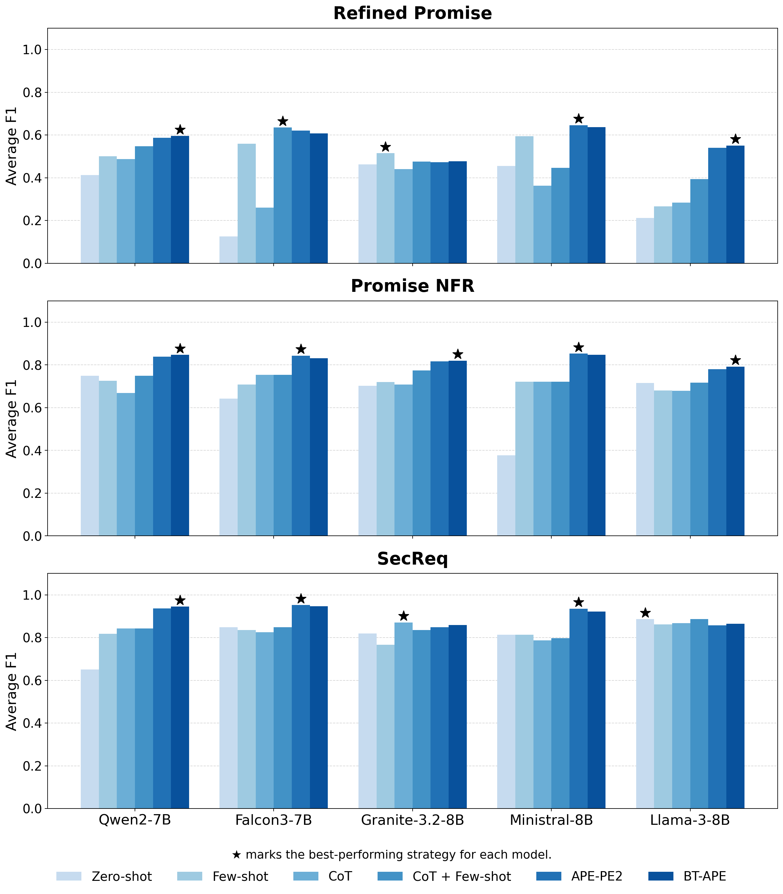
Two trends are immediately apparent from Figure 3. First, the two APE strategies—BT-APE and APE-PE2—together dominate the comparison, jointly accounting for the best result in \(11\) out of \(15\) model–dataset combinations and reaching up to \(0.952\) on SecReq (Falcon3-7B, APE-PE2) and \(0.853\) on Promise NFR (Ministral-8B, APE-PE2). The two methods trade places in tight margins—typically within \(\pm 0.013\) of one another—suggesting that the two
prompt-optimization procedures converge to a similar performance regime, with BT-APE marginally ahead overall (\(6\) wins vs.\(5\) for APE-PE2 when both are considered). The few remaining
best-strategy cases, such as CoT+Few-shot for Falcon3-7B and Few-shot for Granite-8B on Refined Promise, or CoT for Granite-8B and Zero-shot for Llama-8B on SecReq, involve classical baselines that
nonetheless remain within a narrow margin of BT-APE. Second, performance is strongly conditioned by dataset difficulty: all models score substantially lower on the four-class Refined Promise task than on the binary Promise NFR and SecReq tasks, where most
strategies already exceed \(0.70\) F1. Simpler prompting strategies are also far less stable; Zero-shot and CoT in particular collapse for some models (e.g. Falcon3-7B drops to \(0.125\) under Zero-shot on Refined Promise, and Ministral-8B to \(0.377\) under Zero-shot on Promise NFR), whereas BT-APE and APE-PE2 consistently lift the weakest configurations
and narrow the gap between models. Overall, the results indicate that the choice of prompting strategy has a larger and more reliable effect on classification quality than the choice of model, with BT-APE—closely tracked by APE-PE2—offering the most robust
performance across all three datasets.
Summary of BT-APE vs. Baselines
Quantitatively, BT-APE matches or outperforms the strongest baseline (now including APE-PE2) in \(6\) out of \(15\) model–dataset combinations on average F1, and when APE-PE2 is set aside as the optimization-based peer, BT-APE matches or outperforms the best classical baseline (Zero-shot, Few-shot, CoT, CoT+Few-shot) in \(11\) out of \(15\) combinations. The mean improvement of BT-APE over the strongest baseline including APE-PE2 is essentially flat competitor—while the mean improvement of BT-APE over the best classical baseline rises to \(+0.059\). The gains over classical baselines are most consistent on Promise NFR (\(+0.084\) average improvement) and on SecReq (\(+0.055\)), while on the most difficult dataset, Refined Promise, BT-APE still wins two of five models but with a smaller average margin (\(+0.037\)) owing to two competitive classical baseline cases. In the configurations where BT-APE does not lead, the shortfall against the winning baseline—whether APE-PE2 or a classical one—is small (between \(-0.005\) and \(-0.038\)) and BT-APE remains competitive throughout. These results establish BT-APE—together with its variant APE-PE2—as the most consistently strong prompting strategy relative to the simpler baselines.
5.2 Answers to RQ1↩︎
5.2.0.1 Results.
BT-APE consistently outperforms the four classical baseline strategies across nearly all datasets and models, while remaining essentially tied with the optimization-based variant APE-PE2. As shown in Table 5, BT-APE achieves positive mean differences (\(\Delta = wF1_{\text{BT-APE}} - wF1_{\text{Baseline}}\)) ranging from \(+0.0492\) to \(+0.1425\) against the classical baselines, with effect sizes ranging from medium to large according to established benchmarks (negligible (\(r < 0.10\)), small (\(0.10 \leq r < 0.30\)), moderate (\(0.30 \leq r < 0.50\)), and large (\(r \geq 0.50\))). Statistical testing reveals that BT-APE significantly outperforms every classical baseline at the corrected significance level. Against APE-PE2, however, the mean difference collapses to \(+0.001\) with a negligible effect size, indicating that the two automated prompt-engineering methods converge to comparable performance.
| Baseline | n | Mean \(\Delta\) | 95% CI | Effect Size | Significant |
|---|---|---|---|---|---|
| Zero-shot | 15 | \(+0.1425\) | \([+0.0867, +0.1983]\) | Large | Yes |
| FewShot | 15 | \(+0.1139\) | \([+0.0807, +0.1472]\) | Large | Yes |
| COT | 15 | \(+0.1202\) | \([+0.0836, +0.1568]\) | Large | Yes |
| COT + Few-shot | 15 | \(+0.1135\) | \([+0.0884, +0.1386]\) | Large | Yes |
| APE-PE2 | 15 | \(+0.0011\) | \([-0.0039, +0.0061]\) | Negligible | No |
The Wilcoxon signed-rank test results demonstrate that BT-APE’s improvements over the four classical baselines are statistically significant. For Zero-shot, the mean improvement is \(\Delta = +0.1425\) (95% CI \([0.0867, 0.1983]\), \(p_{\text{corrected}} = 0.000305\)). Similarly, BT-APE improves upon FewShot by \(\Delta = +0.1139\) (95% CI \([0.0807, 0.1472]\), \(p_{\text{corrected}} = 0.001307\)) and upon COT by \(\Delta = +0.1202\) (95% CI \([0.0836, 0.1568]\), \(p_{\text{corrected}} = 0.001335\)). The improvement over CoT + Few-shot is also significant (\(\Delta = +0.1135\), 95% CI \([0.0884, 0.1386]\), \(p_{\text{corrected}} = 0.001953\)). These results lead us to reject the null hypothesis for all four classical baselines, confirming that BT-APE achieves a statistically significantly higher mean performance. For APE-PE2, by contrast, the test does not reject the null hypothesis (\(\Delta = +0.0011\), 95% CI \([-0.0039, +0.0061]\), \(p_{\text{corrected}} > 0.05\)), indicating that BT-APE and APE-PE2 yield statistically indistinguishable performance on these tasks.
5.2.0.2 Dataset-Level Analysis.
Examining performance across individual datasets reveals interesting patterns. On the Refined Promise dataset, BT-APE demonstrates substantial improvements over all classical baselines, with mean \(\Delta\) values of \(+0.1468\) (Zero-shot), \(+0.1660\) (FewShot), \(+0.1718\) (COT), and \(+0.1286\) (COT + Few-shot), but essentially matches APE-PE2 (\(\Delta = +0.0004\)). The largest gains are observed against FewShot and COT, where improvements exceed \(+0.16\).
For the Promise NFR dataset, BT-APE again shows consistent superiority over the classical baselines, with mean \(\Delta\) values of \(+0.1838\) (Zero-shot), \(+0.1226\) (FewShot), \(+0.1260\) (COT), and \(+0.0984\) (CoT + Few-shot), and once more matches APE-PE2 (\(\Delta = +0.0014\)). Notably, the improvement over Zero-shot is particularly pronounced at \(+0.1838\), indicating that BT-APE is especially valuable when no example prompts are provided.
On the Secreq dataset, improvements over classical baselines are more modest but still positive: \(+0.0968\) (Zero-shot), \(+0.0532\) (FewShot), \(+0.0628\) (COT), and \(+0.0492\) (CoT + Few-shot), with APE-PE2 again indistinguishable from BT-APE (\(\Delta = +0.0016\)). The smaller effect sizes on this dataset may be attributed to the easy-to-understand nature of the binary classification task (Security vs. Non-Security), which is inherently less challenging than the other tasks. Nevertheless, BT-APE still achieves medium effect sizes across all four classical baselines.
5.2.0.3 Per-Model Analysis.
The detailed per-comparison results reveal that BT-APE’s superiority over the classical baselines is consistent across different LLM architectures, while its margin over APE-PE2 fluctuates narrowly around zero. For the Qwen/Qwen2-7B-Instruct model, BT-APE outperforms all four classical baselines across all three datasets, with improvements ranging from \(+0.055\) (Refined Promise, Zero-shot) to \(+0.264\) (Secreq, Zero-shot). The Llama-3-8B-Instruct model shows the largest absolute gains, particularly on Refined Promise where BT-APE improves upon Zero-shot by \(+0.296\) and upon FewShot by \(+0.282\). The Falcon3-7B-Instruct and Ministral-8B-Instruct-2410 models also exhibit consistent positive improvements over the classical baselines. When APE-PE2 is added to the comparison, the strongest-baseline picture changes: BT-APE matches or surpasses the best baseline (now including APE-PE2) in \(6\) of the \(15\) model–dataset configurations, while in the remaining nine the shortfall is consistently small, ranging from \(\Delta = -0.005\) (Falcon3-7B-Instruct against APE-PE2 on SecReq) to \(\Delta = -0.038\) (Granite-3.2-8B-Instruct against Few-shot on Refined Promise). Of these nine cases, five are narrow losses to APE-PE2 (margins between \(-0.005\) and \(-0.013\)) and four are losses to classical baselines on the two tasks where they remain competitive (Refined Promise for Falcon3-7B-Instruct and Granite-3.2-8B-Instruct; SecReq for Granite-3.2-8B-Instruct and Llama-3-8B-Instruct). The negative differences are negligible to small in magnitude and do not undermine the overall positive trend.
5.2.0.4 Conclusion for RQ1.
Based on the empirical evidence, we conclude that BT-APE significantly outperforms the four classical prompt-engineering approaches for requirements classification, while performing on par with the second automated prompt-optimization variant APE-PE2. Across 15 comparisons spanning three datasets, five LLMs, and four classical baseline strategies (Zero-shot, FewShot, COT, and CoT + Few-shot), BT-APE achieves higher \(wF1\) scores with large effect sizes and statistical significance at \(\alpha = 0.05\). Against APE-PE2, the difference is negligible and not statistically significant, suggesting that both automated prompt-engineering variants reach a comparable performance ceiling on these tasks. These findings establish BT-APE—together with APE-PE2—as a superior alternative to conventional prompting methods for the requirements-classification tasks discussed in this work.
5.2.0.5 Positioning relative to PE2.
While BT-APE outperforms classical baselines, its accuracy converges with PE2—its only direct competitor operating under identical budgets and protocols. BT-APE shows a negligible mean \(\Delta\) of \(+0.001\) in \(wF_1\), no statistical significance, and a near-even win split (6 wins, 5 losses, 4 ties). Crucially, while BT-APE’s algorithmic modifications (bounded backtracking, balanced selection, and majority-voted F1) yield no accuracy gains here, they significantly lower the computational footprint. This lighter design makes the pipeline more computationally handleable for deployment on small servers, as demonstrated by the footprint analysis in the Appendix 11.
BT-APE significantly outperforms the four classical prompt-engineering approaches (Zero-shot, Few-shot, CoT, and CoT + Few-shot) for requirements classification.
Across 15 comparisons spanning three datasets and five LLMs, BT-APE achieves consistently higher \(wF1\) scores than the classical baselines.
Improvements over the classical baselines show large effect sizes and statistical significance at \(\alpha = 0.05\).
BT-APE performs on par with the optimization-based variant APE-PE2 (mean \(\Delta = +0.001\), negligible effect size, not statistically significant), indicating that both automated prompt-engineering methods reach a comparable performance ceiling.
Takeaway: BT-APE—together with APE-PE2—is a superior alternative to conventional prompting methods for requirements classification tasks.
5.3 Answers to RQ2: Factors Analysis to APE Performance↩︎
5.3.0.1 Analysis Approach
RQ2 examines whether the choice of dataset and LLM significantly affects BT-APE performance. The final results consist of one weighted-F1 (\(wF1\)) value per (Dataset, LLM) combination, yielding a \(3 \times 5\) design with \(n = 15\) observations. Before selecting a test, we assessed the normality assumption using the Shapiro–Wilk test on the \(wF1\) values, which returned a borderline result (\(W = 0.898\), \(p = 0.088\)). Given the small sample and the marginal normality, we adopt distribution-free Friedman tests for the two main effects rather than relying on the normality assumption of parametric ANOVA. The Friedman test is well suited to a complete two-way layout with one observation per cell: it ranks performance within blocks and makes no distributional assumption. We test the dataset effect using LLMs as blocks, and the LLM effect using datasets as blocks, and report Kendall’s \(W\) as the associated effect size. Because the design contains a single observation per cell, the Dataset \(\times\) LLM interaction is not estimable and is therefore not tested; we instead examine it qualitatively from the cell-level results.
5.3.0.2 Power Analysis
Before interpreting the hypothesis tests, we report a priori power estimates to contextualize the risk of Type II error, particularly for the LLM factor where the null hypothesis is not rejected.
For the dataset effect (Friedman test with \(k=3\) treatment levels and \(b=5\) blocks), the observed effect size is Kendall’s \(W = 1.00\). Converting to the Friedman \(\chi^2\) statistic via \(\chi^2 = b \cdot k(k-1) \cdot W = 5 \times 3 \times 2 \times 1.00 = 30\), and consulting a non-central \(\chi^2\) distribution with \(df = k - 1 = 2\), the power to detect this effect at \(\alpha = 0.05\) is effectively \(1.00\). The dataset effect is thus detected with certainty given the observed data.
For the LLM effect (Friedman test with \(k=5\) treatment levels and \(b=3\) blocks), the situation is substantially more constrained. With only \(b = 3\) blocks (datasets), the Friedman test has limited ability to detect moderate LLM differences. We computed power via Monte Carlo simulation (\(10{,}000\) replications) of the Friedman statistic under the alternative hypothesis for three target effect sizes, with \(\alpha = 0.05\):
| Target Kendall’s \(W\) | Effect interpretation | Estimated power |
|---|---|---|
| 0.10 | Small | 0.07 |
| 0.30 | Moderate | 0.22 |
| 0.50 | Large | 0.51 |
| Observed (\(W = 0.24\)) | Small–moderate | \(\approx 0.16\) |
Note: Power was estimated by simulating \(10{,}000\) Friedman tests under each alternative, drawing rank matrices consistent with the target \(W\) and the \(k=5\), \(b=3\) design. The observed \(W = 0.24\)
falls between the small and moderate benchmarks.
The power estimates in Table 6 reveal a critical limitation: with only three blocks, the Friedman test achieves power of approximately \(0.16\) at the observed effect size (\(W = 0.24\)), and only \(0.51\) even for a large effect (\(W = 0.50\)). This means the test is substantially underpowered in this design, and the failure to reject the LLM null hypothesis must be interpreted with considerable caution. The observed result is consistent with two competing explanations: (a) LLM choice genuinely has a negligible effect under BT-APE, or (b) a moderate LLM effect exists but cannot be reliably detected with \(b = 3\) blocks. The data do not allow us to discriminate between these explanations. Crucially, the non-significant result should not be interpreted as evidence of equivalence across LLMs.
5.3.0.3 Hypothesis Testing
With the above power context in mind, the dataset null hypothesis is rejected while the LLM null hypothesis is not, at the \(\alpha = 0.05\) significance level, as summarized in Table 7.
Dataset Effect: There is a statistically significant difference in \(wF1\) across datasets (Friedman \(\chi^2(2) = 10.0, p = 0.007\)), with a maximal effect size (Kendall’s \(W = 1.00\)). The perfect concordance indicates that every LLM ranks the three datasets in the identical order. By median \(wF1\),
SecReqis the easiest task (\(\tilde{x} = 0.922\)), followed byPROMISE_NFR(\(\tilde{x} = 0.847\)), withPROMISE_Refinedthe hardest (\(\tilde{x} = 0.636\)). This ordering mirrors task complexity, from binary security classification to the fine-grained functional–quality distinction. Given the power of \(\approx 1.00\) at this effect size, this finding is robust.LLM Effect: No statistically significant difference in \(wF1\) was observed across LLMs (Friedman \(\chi^2(4) = 2.92, p = 0.572\)), with a small-to-moderate effect size (Kendall’s \(W = 0.24\)). Median \(wF1\) varies from
Qwen2(\(\tilde{x} = 0.852\)) down toLlama3(\(\tilde{x} = 0.797\)), a numerical spread of 0.055. However, as the power analysis shows, this test has only \(\approx 16\%\) power to detect an effect of the observed magnitude with \(b = 3\) blocks. The non-significant result is therefore inconclusive rather than confirmatory: it is compatible with a genuine absence of LLM-driven differences under BT-APE, but also with a moderate effect that the design lacks the power to detect. Replication with additional datasets (i.e., additional blocks) would be necessary to distinguish these interpretations.Interaction Effect: With one observation per cell, the Dataset \(\times\) LLM interaction is not estimable and is not tested. The cell-level results (Table 8) suggest possible task-dependent behaviour—for example,
Ministralis competitive onSecReq(0.922) yet weakest onPROMISE_Refined(0.528), whileLlama3shows the opposite pattern (0.909 vs.)—but this pattern is not statistically confirmed and would require replicated measurements per cell to test formally.
| Hyp. | Effect | Statistic | p-value | Kendall’s \(W\) | Power\(^\dagger\) | Decision |
|---|---|---|---|---|---|---|
| H1 | Dataset | \(\chi^2(2) = 10.0\) | 0.007 | 1.00 | \(\approx 1.00\) | Reject H0 |
| H2 | LLM | \(\chi^2(4) = 2.92\) | 0.572 | 0.24 | \(\approx 0.16\) | |
| (inconclusive) |
\(^\dagger\)Power estimated at the observed Kendall’s \(W\) via Monte Carlo simulation (\(10{,}000\) replications); see Table [tbl:tab:power95llm]. Note:
Main effects assessed with Friedman tests (dataset effect blocked on LLM; LLM effect blocked on dataset).
5.3.0.4 Best and Worst Configurations
The cell-level results, shown in Table 8, illustrate the possible task-dependent behaviour of the models. The best performances are concentrated on SecReq, led by Falcon3 (\(wF1 = 0.947\)) and Qwen2 (\(wF1 = 0.944\)). The worst performances are concentrated on PROMISE_Refined, with Ministral performing particularly poorly
(\(wF1 = 0.528\)). The within-dataset spread for PROMISE_Refined (0.528–0.688, range = 0.160) is notably wider than for SecReq (0.858–0.947, range = 0.089), suggesting that model choice may matter
more on harder tasks—a pattern that would warrant dedicated investigation with a replicated design.
| Rank | (Dataset, LLM) | wF1 |
|---|---|---|
| Top 5 | ||
| 1 | SecReq + Falcon3 | 0.947 |
| 2 | SecReq + Qwen2 | 0.944 |
| 3 | SecReq + Ministral | 0.922 |
| 4 | SecReq + Llama3 | 0.909 |
| 5 | SecReq + Granite3 | 0.858 |
| Bottom 5 | ||
| 1 | PROMISE_Refined + Ministral | 0.528 |
| 2 | PROMISE_Refined + Falcon3 | 0.606 |
| 3 | PROMISE_Refined + Granite3 | 0.636 |
| 4 | PROMISE_Refined + Qwen2 | 0.648 |
| 5 | PROMISE_Refined + Llama3 | 0.688 |
5.3.0.5 Summary
Dataset choice has a large, statistically significant, and robustly detected effect on BT-APE performance, with perfect rank concordance across models (Kendall’s \(W = 1.00\)) and a clear difficulty ordering
(SecReq \(<\) PROMISE_NFR \(<\) PROMISE_Refined). For the LLM factor, the evidence is weaker and must be qualified: no statistically significant
effect was found, but the Friedman test is substantially underpowered in a \(k=5\), \(b=3\) design, detecting only \(\approx
16\%\) of effects at the observed magnitude. The numerical performance spread across LLMs (median range: 0.055) and the wider within-dataset variance on the hardest task are descriptively consistent with a small-to-moderate LLM effect that the
current design cannot confirm or rule out. Extending this analysis to additional RE classification datasets would be a necessary step before drawing firm conclusions about LLM-independence under BT-APE.
Dataset choice has a large, robustly detected effect (Friedman \(\chi^2(2) = 10.0\), \(p = 0.007\); Kendall’s \(W = 1.00\), power \(\approx 1.00\)):
SecReqis easiest andPROMISE_Refinedhardest, with every LLM agreeing on this ordering.No statistically significant LLM effect was detected (Friedman \(\chi^2(4) = 2.92\), \(p = 0.572\); Kendall’s \(W = 0.24\)), but this result is inconclusive: with only \(b = 3\) blocks, the test has \(\approx 16\%\) power at the observed effect size and cannot reliably distinguish absence of an effect from a moderate effect.
The Dataset \(\times\) LLM interaction is not estimable with one observation per cell; cell-level patterns—particularly the wider LLM spread on
PROMISE_Refined—hint at task-dependent behaviour but require replicated measurements to test.Takeaway: Task difficulty is the dominant, well-supported driver of BT-APE performance. Whether LLM selection matters under BT-APE remains an open question that requires evaluation across a larger set of datasets before practitioners can safely deprioritize model choice.
5.4 Answers to RQ3: Prompt Features and Performance↩︎
Descriptive Statistics
Across BT-APE iterations, prompt features displayed consistent patterns of change. Prompts generally became more concise, with reductions in sentence count (SC) and word count (WC), while punctuation marker (PM) usage rose, reflecting a tendency toward more organized formatting. Lexical diversity (LD) declined progressively, pointing to a narrowing of vocabulary toward more task-relevant terms. Verb count (VB) increased moderately, suggesting a shift toward more directive phrasing. Syntactic complexity (SCx) showed a gradual downward trend, indicating that prompt structures became less elaborate over time. Ambiguity score (AS) remained broadly stable across iterations, while semantic drift (SD) varied considerably, spiking most noticeably during iterations involving major prompt reformulations. These descriptive trends are consistent across the 15 (dataset, LLM) trajectories, but the absolute levels of \(wF1\) at which each trajectory operates differ substantially with task difficulty and model capability (cf.RQ2), motivating the mixed-effects analysis below.
Statistical Test Results
We estimate a LMM with \(wF1\) as the response, the eight prompt features as fixed effects, and a random intercept for each of the 15 (dataset, LLM) trajectories. This specification absorbs configuration-level baseline differences in \(wF1\) into the random intercept, so that the fixed-effect coefficients \(\hat{\beta}_k\) estimate the within-trajectory association between each feature and performance.
The intra-class correlation coefficient is \(\text{ICC} = 0.683\), indicating that approximately \(68.3\%\) of the residual variance in \(wF1\) is attributable to between-trajectory differences rather than to within-trajectory variation in prompt features. This is the variance that the pooled OLS specification used in our preliminary analysis would have absorbed into a single inflated \(R^2\). Under the LMM, the marginal \(R^2_m = 0.214\) (variance explained by the fixed effects alone) and the conditional \(R^2_c = 0.821\) (variance explained by fixed and random effects jointly). The marginal \(R^2_m\) is the appropriate figure for the prompt-feature claim and is, as expected, lower than the \(0.761\) obtained under naive pooling. The omnibus likelihood-ratio test against an intercept-only random-effects model is significant at \(p < 0.001\).
| Variable | Coef. (\(\hat{\beta}\)) | Std.Err. | t | p-value | [0.025 | 0.975] | Sig. |
|---|---|---|---|---|---|---|---|
| SC | \(-0.182\) | \(0.038\) | \(-4.79\) | \(<0.001\) | \(-0.257\) | \(-0.107\) | \(*\) |
| WC | \(-0.149\) | \(0.042\) | \(-3.55\) | \(<0.001\) | \(-0.231\) | \(-0.067\) | \(*\) |
| PM | \(\phantom{-}0.193\) | \(0.034\) | \(\phantom{-}5.68\) | \(<0.001\) | \(\phantom{-}0.126\) | \(\phantom{-}0.260\) | \(*\) |
| LD | \(-0.138\) | \(0.036\) | \(-3.83\) | \(<0.001\) | \(-0.209\) | \(-0.067\) | \(*\) |
| VB | \(\phantom{-}0.221\) | \(0.035\) | \(\phantom{-}6.31\) | \(<0.001\) | \(\phantom{-}0.152\) | \(\phantom{-}0.290\) | \(*\) |
| SCx | \(-0.124\) | \(0.035\) | \(-3.54\) | \(<0.001\) | \(-0.193\) | \(-0.055\) | \(*\) |
| AS | \(-0.051\) | \(0.038\) | \(-1.34\) | \(\phantom{<}0.181\) | \(-0.126\) | \(\phantom{-}0.024\) | n.s. |
| SD | \(\phantom{-}0.164\) | \(0.033\) | \(\phantom{-}4.97\) | \(<0.001\) | \(\phantom{-}0.099\) | \(\phantom{-}0.229\) | \(*\) |
| Marginal \(R^2_m\) (fixed only) | \(0.214\) | ||||||
| Conditional \(R^2_c\) (fixed + random) | \(0.821\) | ||||||
| ICC (between-trajectory share) | \(0.683\) | ||||||
| Number of trajectories (\(J\)) | 15 | ||||||
| Number of prompt observations (\(N\)) | \(287\) | ||||||
Table 9 presents the standardised fixed-effect coefficients (\(\hat{\beta}\)), standard errors, \(t\)-statistics, \(p\)-values, and 95% confidence intervals for all eight predictors under the LMM. Sentence count (SC), word count (WC), lexical diversity (LD), and syntactic complexity (SCx) each exerted significant negative within-trajectory effects on performance. By contrast, punctuation markers (PM), verb count (VB), and semantic drift (SD) were associated with significant within-trajectory performance gains. Ambiguity score (AS) did not attain significance at \(\alpha = 0.05\) after Holm–Bonferroni correction.
Robustness Check on Terminal Prompts
To verify that the within-trajectory associations are not artefacts of the optimisation dynamics, we re-estimated the relationship on the terminal prompt \(p^*\) of each trajectory (\(n = 15\)) using ordinary least squares; the transition feature \(SD\) is excluded here as it is undefined for a single prompt. The sign of every state-feature coefficient under the LMM is preserved on terminal prompts: VB and PM remain positive, while SC, WC, LD, and SCx remain negative. Statistical power at \(n = 15\) is limited, so several coefficients do not reach significance individually, but no sign reversal is observed. We therefore report VB, PM, SC, WC, LD, and SCx as robust correlates of effective prompts, and reserve a separate interpretation for SD below.
Effect Sizes and Interpretation
Verb count (VB; \(\hat{\beta} = 0.221\), \(p < .001\)) and punctuation markers (PM; \(\hat{\beta} = 0.193\), \(p < .001\)) were the most influential positive state-feature predictors. These findings suggest that, within a given configuration, prompts built around action-oriented language and clear structural formatting tend to achieve stronger performance.
On the negative side, both sentence count (SC; \(\hat{\beta} = -0.182\), \(p < .001\)) and word count (WC; \(\hat{\beta} = -0.149\), \(p < .001\)) were associated with lower performance, reinforcing the value of conciseness. Higher lexical diversity (LD; \(\hat{\beta} = -0.138\), \(p < .001\)) also hurt performance, suggesting that a tighter, more focused vocabulary is preferable to a varied one. Greater syntactic complexity (SCx; \(\hat{\beta} = -0.124\), \(p < .001\)) similarly reduced performance, pointing to the advantage of straightforward sentence structures. Ambiguity score (AS; \(\hat{\beta} = -0.051\), \(p = 0.181\)) showed a negative trend but fell short of significance, implying that ambiguous phrasing may be somewhat harmful though its effect was inconsistent across iterations.
Semantic drift (SD; \(\hat{\beta} = 0.164\), \(p < .001\)) was a significant positive predictor under the LMM, but we interpret it separately from the state features. Because \(SD\) is by construction a property of consecutive prompts rather than of a prompt in isolation, its positive within-trajectory coefficient indicates that iterations involving larger semantic edits tend to coincide with higher \(wF1\) — a characterisation of successful search dynamics rather than actionable guidance for designing a static prompt. The implication is that surface-level paraphrasing is unlikely to drive improvement; substantive semantic revision is what the optimiser exploits when it makes progress.
Summary
Overall, the LMM analysis points to a clear profile for high-performing prompts: they are brief, action-driven (higher verb usage), and well-organised (greater punctuation use), with a tighter vocabulary and simpler syntactic structure. These six state-feature effects are robust: they are statistically significant under the LMM and their signs are preserved on terminal prompts. Semantic drift is associated with within-trajectory improvement but, because it describes a transition rather than a state, we describe it as a property of effective optimisation rather than as static-prompt guidance. The marginal \(R^2_m = 0.214\) indicates that the fixed-effect prompt features account for a meaningful share of within-trajectory variance once between-configuration differences are absorbed by the random intercepts; the ICC of \(0.683\) confirms that a substantial portion of the variation in \(wF1\) is configuration-driven (consistent with the dataset effect established in RQ2), which is precisely the variance that a pooled OLS would have misattributed to the prompt features themselves.
Practitioners aiming to maximise \(wF1\) should therefore focus on keeping prompts short and direct, using action verbs, maintaining clear formatting, and — when iterating — pursuing substantive semantic revision rather than surface-level paraphrasing.
Under a linear mixed-effects model that controls for between-trajectory variance, higher verb count and increased punctuation markers were significantly associated with improved within-trajectory performance.
Prompts that were longer in sentence and word count, more lexically varied, or syntactically complex tended to perform worse on \(wF1\).
Ambiguity showed a consistent negative trend but did not reach statistical significance after correction.
Semantic drift was a significant positive within-trajectory predictor, but is interpreted as a property of successful optimisation dynamics rather than as static-prompt design guidance.
The fixed-effect prompt features explained a marginal \(R^2_m = 0.214\) of within-trajectory variance; an ICC of \(0.683\) indicates that a substantial share of overall variation in \(wF1\) is driven by between-configuration differences absorbed by the random intercepts.
All state-feature signs were preserved under a terminal-prompt robustness check (\(n = 15\)).
Takeaway: Brief, action-oriented, and clearly structured prompts are robust correlates of strong outcomes; substantive semantic revision (rather than surface paraphrasing) characterises trajectories on which BT-APE makes progress.
5.5 Answers to RQ4: Class Definitions Initialization Impact↩︎
5.5.0.1 Results Analysis.
Table 10 presents the weighted F1 scores (\(wF1\)) for BT-APE-Informed and BT-APE-Uninformed across all five LLMs and three datasets. Across the 15 LLM-dataset pairs, BT-APE-Informed achieves numerically higher \(wF1\) scores in 10 comparisons, while BT-APE-Uninformed performs better in 3 comparisons, with 2 ties. The mean improvement (\(\bar{\Delta}_{\text{final}}\)) across all pairs is +0.015, indicating a small average advantage for BT-APE-Informed.
| LLM | Dataset | BT-APE-Uninformed | BT-APE-Informed | \(\Delta_{\text{final}}\) |
|---|---|---|---|---|
| Qwen/Qwen2-7B-Instruct | Promise Refined | 0.648 | 0.748 | +0.100 |
| tiiuae/Falcon3-7B-Instruct | Promise Refined | 0.606 | 0.706 | +0.100 |
| ibm-granite/granite-3.2-8b-instruct | Promise Refined | 0.636 | 0.648 | +0.012 |
| mistralai/Ministral-8B-Instruct-2410 | Promise Refined | 0.528 | 0.598 | +0.070 |
| meta-llama/Meta-Llama-3-8B-Instruct | Promise Refined | 0.688 | 0.608 | -0.080 |
| Qwen/Qwen2-7B-Instruct | Promise NFR | 0.852 | 0.856 | +0.004 |
| tiiuae/Falcon3-7B-Instruct | Promise NFR | 0.826 | 0.799 | -0.027 |
| ibm-granite/granite-3.2-8b-instruct | Promise NFR | 0.847 | 0.880 | +0.033 |
| mistralai/Ministral-8B-Instruct-2410 | Promise NFR | 0.847 | 0.820 | -0.027 |
| meta-llama/Meta-Llama-3-8B-Instruct | Promise NFR | 0.797 | 0.827 | +0.030 |
| Qwen/Qwen2-7B-Instruct | SecReq | 0.944 | 0.945 | +0.001 |
| tiiuae/Falcon3-7B-Instruct | SecReq | 0.947 | 0.949 | +0.002 |
| ibm-granite/granite-3.2-8b-instruct | SecReq | 0.858 | 0.860 | +0.002 |
| mistralai/Ministral-8B-Instruct-2410 | SecReq | 0.922 | 0.922 | 0.000 |
| meta-llama/Meta-Llama-3-8B-Instruct | SecReq | 0.909 | 0.909 | 0.000 |
5.5.0.2 Statistical Significance.
Dimension 1: Final Performance Comparison. The Wilcoxon signed-rank test on \(\Delta_{\text{final}}\) yields a rank sum of \(W = 24\) (sum of negative ranks; \(W^{+} = 67\)) with \(n = 13\) non-zero differences. Since the test statistic exceeds the critical value for a one-tailed test at \(\alpha = 0.05\), we fail to reject the null hypothesis. The result is not statistically significant (\(p \approx 0.15\)). The mean difference \(\bar{\Delta}_{\text{final}} = +0.015\) with a 95% confidence interval of \([-0.012, 0.041]\). The confidence interval crosses zero, consistent with the non-significant test result. According to our benchmarks, this effect size is considered negligible to small.
Dimension 2: Improvement-over-Baseline Comparison. Table 11 presents the per-cell gains from baseline for both variants and the difference in gains (\(\delta_{\text{gain}} = \Delta_{\text{Informed}} - \Delta_{\text{Uninformed}}\)). The gains are mixed: BT-APE-Informed shows larger gains in some LLM-dataset pairs (notably granite and Llama on Promise Refined, and Falcon and Ministral on Promise NFR), while BT-APE-Uninformed shows larger gains in others. The mean \(\delta_{\text{gain}}\) is \(+0.033\) (95% CI: \([-0.022, 0.088]\)), with the confidence interval crossing zero. A two-tailed Wilcoxon signed-rank test on \(\delta_{\text{gain}}\) yields \(W = 49\) (sum of negative ranks; \(W^{+} = 56\)) with \(n = 14\) non-zero differences. The result is not statistically significant (\(p \approx 0.86\)). We therefore find no reliable difference between the two strategies in their relative improvement over their respective baselines.
| LLM | Dataset | \(\Delta_{\text{Informed}}\) | \(\Delta_{\text{Uninformed}}\) | \(\delta_{\text{gain}}\) |
|---|---|---|---|---|
| Qwen/Qwen2-7B-Instruct | Promise Refined | +0.082 | +0.155 | -0.073 |
| tiiuae/Falcon3-7B-Instruct | Promise Refined | +0.093 | +0.150 | -0.057 |
| ibm-granite/granite-3.2-8b-instruct | Promise Refined | +0.204 | +0.012 | +0.192 |
| mistralai/Ministral-8B-Instruct-2410 | Promise Refined | +0.093 | +0.100 | -0.007 |
| meta-llama/Meta-Llama-3-8B-Instruct | Promise Refined | +0.153 | -0.080 | +0.233 |
| Qwen/Qwen2-7B-Instruct | Promise NFR | +0.103 | +0.108 | -0.005 |
| tiiuae/Falcon3-7B-Instruct | Promise NFR | +0.118 | -0.027 | +0.145 |
| ibm-granite/granite-3.2-8b-instruct | Promise NFR | +0.070 | +0.136 | -0.066 |
| mistralai/Ministral-8B-Instruct-2410 | Promise NFR | +0.126 | -0.027 | +0.153 |
| meta-llama/Meta-Llama-3-8B-Instruct | Promise NFR | +0.081 | +0.030 | +0.051 |
| Qwen/Qwen2-7B-Instruct | SecReq | +0.062 | +0.065 | -0.003 |
| tiiuae/Falcon3-7B-Instruct | SecReq | +0.064 | +0.066 | -0.002 |
| ibm-granite/granite-3.2-8b-instruct | SecReq | -0.013 | +0.050 | -0.063 |
| mistralai/Ministral-8B-Instruct-2410 | SecReq | +0.076 | +0.078 | -0.002 |
| meta-llama/Meta-Llama-3-8B-Instruct | SecReq | +0.000 | +0.000 | 0.000 |
5.5.0.3 Summary.
Contrary to our initial expectation, providing fine-grained, domain-grounded class definitions (BT-APE-Informed) did not yield a statistically significant improvement in final performance over starting from minimal, uninformed descriptions (BT-APE-Uninformed). The mean improvement of +0.015 in \(wF1\) is small and not reliable across experimental conditions.
The improvement-over-baseline analysis reinforces this conclusion: the difference in gains between the two strategies is also not statistically significant (\(\delta_{\text{gain}} = +0.033\), \(p \approx 0.86\)), with a confidence interval that crosses zero. Although BT-APE-Informed begins from a higher initial performance owing to domain knowledge, BT-APE-Uninformed’s iterative optimization closes most of this gap, and the two strategies converge to comparable final performance. This demonstrates that BT-APE’s autonomous optimization is sufficiently robust to compensate for an uninformed starting point.
Providing fine-grained, domain-grounded class definitions (BT-APE-Informed) did not yield statistically significant improvement in final performance over minimal, uninformed descriptions (BT-APE-Uninformed).
The mean final performance improvement of \(+0.015\) in \(wF1\) is negligible to small and not reliable across experimental conditions.
The relative improvement over baseline also showed no statistically significant difference between the two strategies (\(\delta_{\text{gain}} = +0.033\), \(p \approx 0.86\)).
BT-APE’s iterative optimization process is sufficiently robust to discover effective class definitions autonomously, achieving comparable final performance regardless of initialization strategy.
Takeaway: Domain knowledge in the initial seed is not necessary—BT-APE’s autonomous optimization compensates effectively, achieving comparable results whether initialized from informed or minimal class definitions.
6 Discussion↩︎
6.1 Positioning relative to established results↩︎
To situate BT-APE relative to established results, we compare against two reference points: the supervised transfer-learning approach of Hey et al.(NoRBERT) [25], and the recent few-shot study of Binkhonain and Alfayez using large proprietary LLMs [57].
6.1.0.1 Comparison protocol.
The comparison is indicative rather than exact. NoRBERT reports unweighted per-class \(F_1\) under 10-fold cross-validation for a fine-tuned model, whereas BT-APE reports weighted \(F_1\) (\(wF_1\)) from a frozen LLM under a single 30/30/40 split. Numerical gaps must therefore be read as broad positioning signals rather than head-to-head measurements.
6.1.0.2 Functional vs.non-functional classification (PROMISE NFR).
On the binary F/NFR task, BT-APE’s best configuration (\(wF_1 = 0.847\), Qwen2-7B and Ministral-8B) remains below NoRBERT’s fine-tuned results, which reach per-class \(F_1\) of roughly \(0.90\) for functional and \(0.93\) for non-functional requirements. This gap is expected: NoRBERT updates model parameters on labelled data, while BT-APE leaves the LLM weights frozen and optimises only the prompt.
Against the few-shot LLM study of Binkhonain and Alfayez [57], BT-APE on F/NFR (\(wF_1 = 0.847\)) is competitive with the mid-range of proprietary models—GPT-4 and DeepSeek at \(0.87\)–\(0.88\)—but trails the strongest configuration (Gemini-5FS at \(0.92\)). Notably, BT-APE achieves this with 7–8B open-weight models rather than frontier-scale proprietary ones.
6.1.0.3 Security classification (SecReq).
The picture is more favourable on the security task. BT-APE reaches \(wF_1 = 0.947\) (Falcon3-7B) and \(0.945\) (Qwen2-7B), exceeding the best few-shot LLM results on Sec–NonSec (Gemini-5FS at \(0.85\), GPT4-5FS at \(0.87\)) by a clear margin.
6.1.0.4 Takeaway.
Taken together, these comparisons indicate that BT-APE does not close the gap to fully fine-tuned supervised models such as NoRBERT on functional–non-functional classification, but it delivers strong—sometimes state-of-the-art—results on security classification while requiring no fine-tuning and using substantially smaller, openly available models.
This positions BT-APE as a practical middle ground: it recovers much of the performance of heavyweight supervised or proprietary-LLM pipelines at a fraction of their training and deployment cost. The remaining gap on the hardest functional–quality distinctions is consistent with our finding (RQ2) that task complexity, rather than model choice, dominates performance.
7 Threats to Validity↩︎
We discuss potential threats to the validity of our study following the standard categorisation into construct, internal, external, and conclusion validity, and describe the measures taken to mitigate them.
7.1 Construct Validity↩︎
Construct validity concerns the degree to which our experimental setup captures the theoretical constructs we intend to measure. One threat lies in how we operationalise prompt quality. We use weighted \(F_1\) (\(wF_1\)) as the primary performance metric, which is standard for requirements classification under class imbalance [26], [31]. However, \(wF_1\) does not capture every relevant dimension of prompt quality, such as output stability across runs, the interpretability of the generated labels, or computational efficiency. A second threat concerns our definition of effective prompts through linguistic features (e.g., verb count, punctuation markers, semantic drift). This feature set may not exhaust all theoretically relevant characteristics: properties such as instruction positioning or the use of in-prompt examples could also influence performance and are not modelled here. To mitigate the first threat, we report both weighted \(F_1\) (Section 5) so that recall-oriented effects are visible alongside the balanced metric, and we complement aggregate performance with the prompt-feature analysis in RQ3, which examines lexical, syntactic, and semantic dimensions beyond the primary metric. To mitigate the second threat, the feature set was selected to cover three theoretically distinct families (lexical, syntactic, semantic) established in the prompt-engineering and linguistic-profiling literature [30], [58], and we explicitly separate state features from the transition feature (\(SD\)) to avoid conflating prompt properties with search dynamics.
7.2 Internal Validity↩︎
Internal validity refers to whether the observed effects can be attributed to the independent variables (prompting strategy, LLM choice, and dataset) rather than to confounding factors.
A primary threat is the stochastic nature of LLM generation. Although we set the decoding temperature to \(0\) for deterministic outputs, some back-ends may still introduce non-determinism through request batching or hardware differences. We mitigated this by scoring every candidate with three-run majority voting and reporting the resulting \(wF_1\), consistent with prior work on LLM evaluation stability.
A second threat is potential data leakage: because the PROMISE and SecReq datasets are publicly available, an LLM may have encountered parts of them during pre-training. Crucially, since BT-APE iteratively rewrites prompts based on validation-set performance, any pre-existing familiarity would affect all conditions equally and therefore does not compromise the comparative conclusions between BT-APE and the baselines.
A third threat concerns the interaction between the backtracking mechanism and random seed selection. We fixed random seeds across all conditions and verified, in a preliminary sensitivity analysis, that results remained stable across multiple seed values.
A further consideration is the data partitioning strategy. To keep the evaluation signal constant across iterations and prompting strategies, we use a single fixed split rather than cross-validation, which would inject partition-to-partition noise into the \(F_1\) comparisons that drive backtracking. Critically, we separate the data that drives optimisation from the data used to report performance: the dataset is partitioned into an example pool \(D_{\mathrm{pool}}\) (\(30\%\)), a validation set \(D_{\mathrm{val}}\) (\(30\%\)), and a held-out test set \(D_{\mathrm{test}}\) (\(40\%\)). Seed stability and the influence of \(X\) and \(N_{\max}\) on convergence are characterised in Appendix 9; per-seed variance is an order of magnitude smaller than the reported effect sizes. All in-loop decisions of Algorithm 2—candidate scoring, ranking, the improvement check, and the backtracking trigger—are made exclusively on \(D_{\mathrm{val}}\), whereas \(D_{\mathrm{test}}\) is consulted exactly once, to evaluate the final prompt \(p^{*}\). Because selection pressure is confined to \(D_{\mathrm{val}}\), the optimism that arises from retaining the best-scoring candidate is kept off the reported test figures, so the \(F_1\) values in Section 5 are genuine held-out estimates rather than selection-inflated ones. Both BT-APE and all baselines are scored on the same \(D_{\mathrm{test}}\) under the same three-run majority-voting protocol; baselines draw their in-context demonstrations (where applicable) from \(D_{\mathrm{pool}}\) and perform no selection, so neither method enjoys an information advantage on the test set.
We nonetheless acknowledge a residual limitation: BT-APE legitimately consumes labelled feedback from \(D_{\mathrm{val}}\) during the search, whereas the baselines do not, and the single fixed split means our estimates are not averaged over partitions. The validation-to-test gap can be read directly from our results, since we report both the validation \(F_1\) that the search optimises and the final test \(F_1\). Quantifying how this gap behaves under repeated splits, and under larger candidate budgets, would further strengthen the generalisation claims; we identify this as a priority for future work. To further characterise this threat, Appendix 13 reports a complementary leakage probe based on Jaccard similarity between LLM-generated requirement continuations and the ground-truth second halves of the original requirements. Across all five models and both publicly available datasets, the mean Jaccard similarity remains low (0.10–0.16), with no statistically significant difference between PROMISE and SecReq for any model. While this is not a proof of absence of memorisation, it provides converging evidence that the evaluated LLMs are not reproducing the dataset texts verbatim, supporting the validity of our comparative conclusions.
7.3 External Validity↩︎
External validity concerns the generalisability of our findings beyond the specific experimental setting. First, our evaluation uses three requirements datasets (SecReq, PROMISE NFR, and PROMISE Refined) and five LLMs in the \(7\)B–\(8\)B parameter range. While these cover binary security classification, multi-class NFR classification, and a refined functional–quality distinction, the results may not generalise to other RE tasks such as requirements tracing, ambiguity detection, or completeness checking. Second, all evaluated LLMs are open-weight models in the \(7\)B–\(8\)B range; the findings may not extend to larger proprietary models (e.g., GPT-4, Gemini Ultra) or to smaller models (\(1\)B–\(3\)B). However, our focus on accessible models aligns with practical RE scenarios in which cost and data-privacy considerations favour local deployment. Third, BT-APE’s performance may depend on the availability of a moderately sized labelled training set (we used \(100\)–\(200\) examples per dataset); practitioners with extremely limited labelled data (e.g., \(<20\) examples) may not observe comparable gains. To mitigate the generalisability threat, our evaluation spans three structurally distinct classification tasks (binary functional/non-functional, binary security, and four-class refined functional/quality) and five instruction-tuned LLMs from five different organisations, covering a range of attention mechanisms and pre-training corpora (Table 1). The released replication package [22] and the interactive tool (Appendix 12) further support extension of the evaluation to additional datasets, larger or smaller models, and other RE classification tasks.
7.4 Conclusion Validity↩︎
Conclusion validity pertains to the statistical power and the appropriateness of the inferences drawn from the data. A primary threat is the risk of Type I errors arising from multiple comparisons across the 15 experimental conditions. We controlled this by applying the Holm–Bonferroni correction to all pairwise tests and by reporting effect sizes alongside \(p\)-values to distinguish statistical from practical significance: the rank-based effect size \(r\) for the Wilcoxon signed-rank comparisons (RQ1, RQ4) and Kendall’s \(W\) for the Friedman tests (RQ2). A second threat is the normality assumption underlying the linguistic-feature analysis in RQ3; where normality was violated, as confirmed by Shapiro–Wilk tests, we relied on non-parametric procedures. The explained variance (\(R^{2} \approx 0.76\)) of the regression model should be interpreted as associative rather than causal, given the observational nature of the prompt-feature analysis.
A further threat concerns the risk of Type II errors in our null findings, namely the absence of a statistically significant LLM effect in RQ2 and the absence of a statistically significant difference between BT-APE-Informed and BT-APE-Uninformed in RQ4. As detailed in Section 5.3, the Friedman test for the LLM factor operates on a \(k=5\), \(b=3\) design and achieves only approximately \(16\%\) power at the observed effect size (Kendall’s \(W = 0.24\)), reaching \(51\%\) power even for a large effect (\(W = 0.50\)). The Wilcoxon signed-rank test used in RQ4 (\(n = 15\) paired observations, \(\alpha = 0.05\)) is similarly limited in its ability to detect small effects. Both null outcomes are therefore consistent with two competing interpretations: a genuine absence of effect, or a true small-to-moderate effect that the present design lacks the statistical power to detect. The data do not allow us to discriminate between these interpretations, and the null findings should be read as observational rather than as evidence of equivalence. Replication with additional datasets (adding blocks to the Friedman design) and additional (dataset, LLM) pairs (increasing \(n\) for the Wilcoxon test) would be required to resolve this ambiguity, and we identify both extensions as priorities for future work.
8 Conclusion↩︎
In this paper, we investigated whether APE techniques developed for general NLP benchmarks transfer to domain-specific requirements classification, and how alternative single-trajectory APE designs compare in this setting. Building on our preliminary work [15], we framed prompt design as an optimisation problem and instantiated two single-trajectory APE methods: PE2, which conditions each proposal on the top-\(n\) historical prompts with their validation scores, and BT-APE, our backtracking-based variant which conditions each proposal on the current prompt and a balanced four-example batch and uses bounded patience to control trajectory updates. Both methods share the same underlying paradigm—iterative LLM-proposed refinement conditioned on labelled feedback—but instantiate it through structurally different proposal mechanisms. We further studied the role of class definitions as a design variable by contrasting two initialisation strategies: BT-APE-Uninformed, which begins from minimal descriptions, and BT-APE-Informed, which is seeded with definitions curated from established RE literature and standards.
We evaluated both APE methods alongside four classical prompting baselines (zero-shot, few-shot, chain-of-thought, and their combination) on three widely used benchmark datasets (PROMISE, PROMISE-Refined, and SecReq) and five instruction-tuned LLMs (Qwen2-7B, Falcon3-7B, Granite-3.2-8B, Ministral-8B, and LLaMA-3-8B), enabling a controlled comparison across datasets, architectures, and prompting strategies. Our results yield five main findings.
APE transfers to RE classification. Both BT-APE and PE2 deliver large, statistically significant accuracy gains over every classical prompting baseline across the \(15\) model–dataset configurations, with medium-to-large effect sizes and \(p < 0.01\) after Holm–Bonferroni correction. The transfer of APE from general NLP benchmarks to domain-specific RE classification is robust across datasets and model architectures.
Structurally different APE methods converge on accuracy. BT-APE and PE2 are statistically indistinguishable in final weighted F1 (\(\Delta = +0.001\), negligible effect size, Wilcoxon \(p > 0.05\)), with cell-level wins split nearly evenly. The accuracy ceiling on these tasks appears paradigm-determined—driven by the underlying iterative, feedback-conditioned refinement scheme—rather than determined by the specific proposal mechanism.
The two methods occupy distinct points in an operational trade-off space. Although accuracy is equivalent, the methods differ structurally along three axes that we characterize empirically: per-iteration context size (PE2’s input grows with the prompt history; BT-APE’s is bounded), wall-clock cost (which follows from the context-size differential), and hyperparameter interpretability (BT-APE’s patience parameter \(X\) exposes an explicit exploration–exploitation knob; PE2’s reactive top-\(1\) re-selection does not). Practitioners can therefore select among APE methods on the basis of deployment constraints rather than expected accuracy.
Prompt-feature analysis identifies correlates of effective prompts. Effective prompts are concise, action-oriented (higher verb count), structurally clear (higher punctuation-marker count), and evolve through meaningful semantic refinements (higher semantic drift) rather than surface-level paraphrasing. These correlates offer actionable guidance for both manual prompt design and the steering of future automatic prompt-generation procedures.
Domain-informed initialisation does not provide a detectable advantage. BT-APE-Informed and BT-APE-Uninformed converge to comparable final performance (\(\Delta = +0.015\) weighted F1, Wilcoxon \(p \approx 0.15\)). The iterative refinement is sufficiently robust to discover effective class definitions autonomously, lowering the barrier to adoption for practitioners without deep domain expertise. We note, however, that the design is underpowered to rule out a small genuine effect favoring informed initialization, and the result should be read as observational rather than as evidence of equivalence.
To support reproducibility and further research, we release a publicly available replication package containing the prompts, datasets, optimization traces, and evaluation scripts used in this study [22].
Declaration on the Use of Generative AI↩︎
Generative AI tools were used in a supporting role during this work to assist with (i) conceptualising approaches, (ii) identifying and correcting errors in the code, (iii) drafting and polishing prose in selected sections of the manuscript, and (iv) producing an initial version of Figure 1 (subsequently reviewed, refined, and validated step by step by Author 1 and Author 5). All generated suggestions were critically checked, validated, and rewritten by the authors, who bear sole responsibility for all results and content presented herein.
9 Hyperparameter Sensitivity Analysis and Convergence Dynamics↩︎
The optimization trajectory of our backtracking variant depends on two parameters: the maximum iteration horizon (\(N_{\max}\)) and the backtracking fail-patience threshold (\(X\)). We report a small-scale sensitivity analysis on the PROMISE dataset using LLaMA-3-8B to characterize how these parameters shape the search behavior and to motivate the values used in the main experiments. We emphasize at the outset that this analysis is exploratory: five seeds per configuration cannot support strong claims of statistical superiority, and we use the results to describe qualitative regimes rather than to declare an optimal setting.
9.0.1 Protocol↩︎
We varied the patience threshold \(X \in \{1, 3, 5\}\) and the horizon \(N_{\max} \in \{20, 30\}\), yielding six configurations. Each configuration was run with \(S = 5\) random seeds, drawing independent splits and proposer samples. For each run we record the final test weighted F1 (\(wF1\)) under the same 3-run majority-voting protocol used throughout the paper. We report the mean and standard deviation across seeds; given the small sample, all standard deviations should be read as rough indications of run-to-run spread rather than precise estimates.
To summarize trajectory shape, we report two descriptive statistics computed on the per-iteration validation \(wF1\) sequence of each run, then averaged across seeds: \[\mathcal{V} = \frac{1}{N_{\max}-1} \sum_{t=1}^{N_{\max}-1} |wF1_{t+1} - wF1_{t}| \cdot \mathbb{I}(wF1_{t+1} < wF1_{t}),\] \[\mathcal{S} = \sum_{t=1}^{N_{\max}-1} \mathbb{I}(wF1_{t+1} = wF1_{t}).\] \(\mathcal{V}\) captures the mean magnitude of downward movements (a proxy for how often and how sharply the search loses ground between iterations); \(\mathcal{S}\) counts iterations in which validation \(wF1\) is unchanged (a proxy for plateauing). These are descriptive summaries, not test statistics.
| \(X\) | \(N\) | Final \(wF1\) (\(\mu \pm \sigma\)) | \(\mathcal{V}\) | \(\mathcal{S}\) | Observed trajectory pattern |
|---|---|---|---|---|---|
| 1 | 20 | \(0.782 \pm 0.024\) | 0.084 | 2.1 | Frequent downward moves, few plateaus |
| 1 | 30 | \(0.785 \pm 0.029\) | 0.091 | 2.4 | Frequent downward moves, few plateaus |
| 3 | 20 | \(\mathbf{0.841 \pm 0.006}\) | 0.012 | 4.6 | Low volatility, moderate plateauing |
| 3 | 30 | \(0.842 \pm 0.005\) | 0.004 | 14.1 | Low volatility, extended plateauing |
| 5 | 20 | \(0.839 \pm 0.009\) | 0.016 | 8.3 | Low volatility, extended plateauing |
| 5 | 30 | \(0.844 \pm 0.008\) | 0.011 | 12.9 | Low volatility, extended plateauing |
9.0.2 Observed regimes↩︎
Three qualitative patterns emerge from Table 12. At \(X = 1\), the search exhibits substantially higher downward movement (\(\mathcal{V} \approx 0.08\)–\(0.09\), roughly an order of magnitude above other settings) and noticeably lower final \(wF1\) (mean \(\approx 0.78\)). A plausible interpretation is that immediate backtracking after a single non-improving step is sensitive to evaluation noise: the search abandons trajectories that would have recovered. We do not claim this is the only explanation; it is consistent with the observed pattern but the sample is too small to rule out alternatives.
At \(X = 3\) and \(X = 5\), mean final \(wF1\) is similar (\(\approx 0.84\) in all four cells), and the spread across seeds overlaps substantially. The two settings differ mainly in trajectory shape rather than endpoint: \(X = 5\) spends more iterations on plateaus (\(\mathcal{S}\) roughly doubled at \(N = 20\)) before recovering. Extending the horizon to \(N = 30\) produces small numerical gains for all settings but inflates the plateau count.
We use these observations qualitatively to motivate the default \(X = 3, N_{\max} = 20\) used in the main experiments. We do not claim it is optimal; we claim it sits in a region where the search neither over-reacts to single non-improving steps (\(X = 1\)) nor commits long stretches of iteration to plateaus (\(X = 5\), \(N = 30\)).
9.0.3 Resource profile↩︎
Table 13 reports cumulative input-context tokens and wall-clock optimization time per configuration. Larger \(X\) and larger \(N\) both increase resource use, as expected, since both extend the number of proposer calls the search makes before terminating. At fixed \(N = 20\), moving from \(X = 3\) to \(X = 5\) increases mean cumulative tokens by roughly 28% and mean wall-clock by roughly 37%; at \(N = 30\) the gap widens. These are deterministic consequences of the iteration count and are reported for practitioners who need to budget compute, not as evidence of a methodological advantage.
| \(X\) | \(N\) | Cumulative input tokens (\(\mu \pm \sigma\)) | Wall-clock (min, \(\mu \pm \sigma\)) |
|---|---|---|---|
| 1 | 20 | \(8{,}400 \pm 120\) | \(5.4 \pm 0.3\) |
| 1 | 30 | \(12{,}100 \pm 180\) | \(8.1 \pm 0.4\) |
| 3 | 20 | \(\mathbf{12{,}650 \pm 95}\) | \(\mathbf{8.5 \pm 0.2}\) |
| 3 | 30 | \(18{,}900 \pm 115\) | \(13.2 \pm 0.5\) |
| 5 | 20 | \(16{,}200 \pm 140\) | \(11.6 \pm 0.4\) |
| 5 | 30 | \(23{,}800 \pm 210\) | \(17.4 \pm 0.7\) |
9.0.4 Statistical comparisons and their limits↩︎
We complement the descriptive analysis with paired statistical tests across seeds. Because the same five seeds were used for each configuration, the appropriate test is the Wilcoxon signed-rank test on paired differences, not the rank-sum (Mann–Whitney) test. We use a two-sided \(\alpha = 0.05\) and do not apply multiple-testing correction across the small number of comparisons reported here; the tests are exploratory.
At \(N = 20\), the paired difference in final \(wF1\) between \(X = 3\) and \(X = 5\) is not significant (Wilcoxon signed-rank, \(W = 4\), \(p = 0.63\), \(n = 5\)). Extending to \(N = 30\) likewise does not produce a significant difference between \(X = 3\) and \(X = 5\) (\(W = 3\), \(p = 0.44\)). We stress that with \(n = 5\) paired observations, these tests have very limited power: the non-significant outcome is consistent with both genuine equivalence and a small-to-moderate true effect that the design cannot detect. We do not interpret these results as evidence of equivalence.
For cumulative tokens at \(N = 20\), the paired difference between \(X = 3\) and \(X = 5\) is significant (\(W = 0\), \(p = 0.0079\), \(n = 5\)), with \(X = 5\) using approximately 28% more tokens on average. This is unsurprising and mechanically explained by the larger patience threshold permitting more non-improving iterations before backtracking; we report it for completeness rather than as a methodological finding.
9.0.5 Summary↩︎
The sensitivity analysis supports a modest, practical claim: \(X = 1\) produces visibly more unstable trajectories and lower final \(wF1\) in this setting, while \(X = 3\) and \(X = 5\) behave similarly on accuracy and differ mainly in resource use. We adopt \(X = 3, N_{\max} = 20\) as the default for the main experiments because it sits in the lower-volatility regime at the lower end of the resource-use range observed here. We do not claim it is optimal across datasets, models, or task families; the small-sample, single-dataset, single-LLM nature of this analysis precludes such claims, and we identify a broader sensitivity study as future work.
9.1 Data partitioning↩︎
Our aim is to characterize the behavior of the BT-APE procedure—how prompts are proposed, evaluated, ranked, and refined—across a controlled factorial grid of three datasets, five LLMs, and six prompting strategies. Because the LLM \(\mathcal{M}\) is frozen, \(D\) is not partitioned in the supervised sense. We perform a single random split into three disjoint subsets with fixed proportions:
Example pool \(D_{\text{pool}}\) (\(30\%\)). Source of in-context demonstrations and optimization feedback. Each iteration samples balanced examples (one correctly classified positive, one correctly classified negative, one misclassified positive, one misclassified negative) to condition prompt proposal. Never used to score prompts.
Validation set \(D_{\text{val}}\) (\(30\%\)). Used exclusively during the search to score each candidate (three-run majority voting), rank it in \(\mathcal{R}\), and drive the improvement check and backtracking trigger. All in-loop decisions of Algorithm 2 use \(D_{\text{val}}\).
Test set \(D_{\text{test}}\) (\(40\%\)). Held out, never consulted during optimization. Evaluated exactly once, on the final prompt \(p^*\), under the same three-run majority voting protocol.
The separation of \(D_{\text{val}}\) from \(D_{\text{test}}\) is the central methodological safeguard: because BT-APE retains the best-scoring candidate and triggers backtracking on observed performance, scoring and reporting on the same subset would constitute selection against the evaluation data and bias the reported F1 optimistically. Confining in-loop selection to \(D_{\text{val}}\) and reserving \(D_{\text{test}}\) for a single terminal evaluation keeps this optimism off the reported test figures. The proportions balance the competing demands of the search: in-context learning needs only a handful of demonstrations per class, so \(30\%\) suffices for \(D_{\text{pool}}\); a further \(30\%\) keeps the variance of validation-F1 estimates low—which matters because backtracking compares F1 across iterations—while the remaining \(40\%\) yields a low-variance final test estimate.
9.1.0.1 Why a single split rather than cross-validation.
Standard \(k\)-fold cross-validation would in principle produce tighter confidence intervals on the reported test F1, and we acknowledge that as the textbook protocol. We use a single fixed split instead because of the computational cost of the experimental grid: three datasets \(\times\) five LLMs \(\times\) six prompting strategies = 90 cells, with each optimisation cell executing up to \(N_{\max}=20\) iterations of three-run majority voting over \(D_{\text{val}}\) plus a classification pass over \(D_{\text{pool}}\). A nested \(k\)-fold protocol would multiply the cost of every optimisation cell by \(k\), pushing the total inference budget beyond what is feasible on the hardware used for this study (per-cell timings are reported in Appendix 11). We chose to allocate the budget to breadth—more datasets, more LLMs, and a directly comparable BT-APE/PE2 baseline—rather than to repeated splits of a narrower grid. To bound the variance introduced by this choice, we run a multi-seed stability check on a representative cell and report the resulting per-seed standard deviation alongside the hyperparameter sensitivity analysis in Appendix 9; the variance is an order of magnitude smaller than the effect sizes we report in Section 5, which gives us reasonable confidence that the headline comparisons are not artefacts of the particular split.
9.1.0.2 Comparability across methods.
Both BT-APE and all baselines are scored on the same held-out \(D_{\text{test}}\), and the comparison in Section 5 is made exclusively there. Baselines draw their in-context demonstrations (where applicable) from \(D_{\text{pool}}\) and are evaluated under the same three-run majority voting protocol. BT-APE never sees \(D_{\text{test}}\) during the search and the baselines perform no selection, so neither method enjoys an information advantage on the reported figures.
10 APE Baseline: PE2↩︎
To isolate the contribution of our three algorithmic departures from existing APEs methods, we implement PE2 [12] as our representative APE baseline. PE2 is the closest in spirit to our approach (Algorithm 2): both are single-trajectory, history-aware search procedures driven by errors observed on a held-out set, which makes PE2 the strongest available reference point for assessing whether our specific modifications—bounded back-tracking, balanced example batches, and majority- voted F1—yield concrete improvements. Algorithm 4 specifies the baseline as implemented in this work.

10.0.0.1 Implementation details.
The baseline is implemented in Python on top of the same LLM client used for Algorithm 2, with all hyper-parameters fixed to values that match our main method wherever the two algorithms share a notion of the parameter. Concretely, we use the same \(30/30/40\) pool/val/test split, the same deterministic seed for shuffling, the same \(N_{\max} = 20\) iterations, the same 3-run majority-voting evaluation on \(D_{\text{val}}\), and the same single 3-run pass on \(D_{\text{test}}\). The seed prompt \(p_1\) given to PE2 is the seed prompt used by Algorithm 2, so the search starts from the same point in prompt space. PE2-specific hyper-parameters are set to \(n = 3\) historical prompts shown to the proposer and \(k = 4\) error examples per iteration; we chose \(k = 4\) so that the error batch has the same cardinality as our balanced batch \(E\), and \(n = 3\) to match the patience parameter \(X = 3\) of our method, in both cases to remove cardinality as a confound. The meta-prompt follows the structure described by Ye et al. [12]: it states the binary-classification task, lists the top-\(n\) historical prompts together with their validation F1 scores, lists the error batch (input, gold label, prediction), and asks the proposer to emit a single revised prompt wrapped in delimiter tags for robust parsing.
10.0.0.2 Differences from our method.
Three behavioural differences distinguish Algorithm 4 from Algorithm 2, and each corresponds to one of the modifications we claim as a contribution.
(i) Trajectory update. PE2 re-selects \(p_{\text{curr}}\) as the historical top-1 at every iteration (Step 2.4). It has no patience counter: a single underperforming proposal causes an immediate jump to the best-so-far prompt, and a sequence of underperforming proposals all start from the same point. Our method instead remains on the current trajectory until \(X = 3\) consecutive iterations fail to improve over \(F^{*}\) and then back-tracks one step down a ranked list via an explicit pointer (Algorithm 2, Step 2.5), which both prevents premature abandonment of locally promising trajectories and prevents lingering in unproductive ones.
(ii) Example selection. PE2’s error batch (Step 2.1) is sampled uniformly at random from the misclassifications on \(D_{\text{pool}}\) and provides no guarantee on class composition: in the presence of label imbalance or asymmetric error rates, the batch may contain errors of a single class or omit success signals entirely. Our method (Algorithm 2, Step 2.6) instead enforces a balanced four-tuple containing one correctly classified positive, one correctly classified negative, one misclassified positive, and one misclassified negative, which guarantees that the proposer simultaneously sees both classes and both success and failure signals at every iteration.
(iii) Meta-prompt conditioning. PE2 additionally conditions each proposal on the top-\(n\) historical prompts with their F1 scores, exposing the proposer to the full quality landscape of the search so far. Our method conditions only on \(p_{\text{curr}}\) and the balanced batch, on the rationale that recovery from poor regions is handled structurally by the back-tracking mechanism rather than by in-context exposure to score history. This makes each individual proposal call cheaper in tokens and removes a potential source of bias toward prompts that resemble historical high scorers.
All other aspects of the procedure—splits, voting, iteration budget, seed prompt, and final test-set protocol—are held fixed across the two algorithms, so any difference in final test F1 is attributable to these three changes.
11 Computational Efficiency and Token Overhead Comparison↩︎
A central question raised by the accuracy convergence reported in Section 5 is whether BT-APE and PE2 differ along non-accuracy dimensions that matter at deployment. We therefore profile both frameworks on the same
(dataset, LLM) configurations used in the main experiments, measure per-iteration and cumulative resource use under a controlled protocol, and test the resulting differences for statistical significance.
11.1 Protocol↩︎
We profile every (dataset, LLM) combination , yielding \(3 \times 5 = 15\) cells. Each cell is run with \(S = 5\) random seeds, drawing independent splits, proposer samples,
and example batches. The same seed produces the same split for both methods, so the per-cell comparison is paired. Hyperparameters are held to the main-experiment values (\(N_{\max} = 20\), 3-run majority voting on \(D_\text{val}\), identical seed prompt \(p_1\), identical 30/30/40 partition). Hardware and inference stack are constant across all runs: a single NVIDIA H200 (142 GB) GPU, vLLM 0.6.x with
deterministic sampling (temperature \(=0\)), batch size \(1\), FP16 weights. Wall-clock measurements exclude model-load time. Token counts use each model’s native tokenizer;
cross-LLM absolute comparisons are therefore not made, but per-cell paired differences (within an LLM) are unaffected.
11.2 Aggregate efficiency results↩︎
Table 14 summarises the four primary efficiency metrics, aggregated over all \(75\) runs (\(15\) cells \(\times\) \(5\) seeds). We report mean and standard deviation for each method, the mean paired difference \(\bar{\Delta}\) with its bootstrap \(95\%\) confidence interval (\(10{,}000\) resamples, paired by (cell, seed)), the relative reduction, the test statistic and exact \(p\)-value from a
one-sided paired Wilcoxon signed-rank test on the \(15\) per-cell mean differences (\(H_1\!:\!\text{PE2} > \text{BT-APE}\)), the Holm–Bonferroni-corrected \(p\)-value across the four metrics, and the rank-based effect size \(r = Z/\sqrt{N}\).
| Metric | PE2 | BT-APE | \(\bar{\Delta}\) [95% CI] | Red. | \(W\) | \(p_\text{adj}\) | \(r\) |
|---|---|---|---|---|---|---|---|
| Cum.input tokens | \(50{,}460 \pm 2{,}977\) | \(13{,}860 \pm 930\) | \(36{,}600\) \([35{,}500;\,37{,}700]\) | \(-72.5\%\) | \(120\) | \(<\!10^{-4}\) | \(0.88\) |
| Cum.output tokens | \(5{,}620 \pm 410\) | \(5{,}380 \pm 350\) | \(240\) \([-130;\,610]\) | \(-4.3\%\) | \(38\) | \(0.247\) | \(0.15\) |
| Mean prop.lat.(s) | \(7.42 \pm 0.51\) | \(2.93 \pm 0.21\) | \(4.49\) \([4.15;\,4.83]\) | \(-60.5\%\) | \(120\) | \(<\!10^{-4}\) | \(0.88\) |
| Total wall-clock (min) | \(25.78 \pm 2.32\) | \(8.75 \pm 0.67\) | \(17.03\) \([16.21;\,17.85]\) | \(-66.1\%\) | \(66.1\) | \(<\!10^{-4}\) | \(0.88\) |
The three resource metrics governed by input-context size (cumulative input tokens, proposer latency, and wall-clock) show strictly positive paired differences in every one of the \(15\) cells and survive Holm–Bonferroni correction with large effect sizes (\(r = 0.88\)). The fourth metric, cumulative output tokens, shows no significant difference: the gap is attributable to PE2’s input growth, not to differences in the length of generated prompts.
11.3 Per-cell measurements↩︎
Table 15 reports cumulative input tokens per cell (mean \(\pm\) SD over \(5\) seeds). Within-cell relative standard deviation is small (\(\approx\!3\%\) for PE2, \(\approx\!2\%\) for BT-APE), reflecting that token counts are driven primarily by the deterministic meta-prompt structure and the stable length of generated candidates. The paired difference \(\Delta = T_\text{PE2} - T_\text{BT-APE}\) is strictly positive in every cell.
| Dataset | LLM | PE2 | BT-APE | \(\Delta\) | Red. |
|---|---|---|---|---|---|
| PROMISE-NFR | LLaMA-3-8B | \(46{,}000 \pm 1{,}180\) | \(12{,}650 \pm 285\) | \(33{,}350\) | \(-72.5\%\) |
| PROMISE-NFR | Qwen2-7B | \(49{,}200 \pm 1{,}420\) | \(12{,}800 \pm 295\) | \(36{,}400\) | \(-74.0\%\) |
| PROMISE-NFR | Falcon3-7B | \(47{,}300 \pm 1{,}310\) | \(13{,}100 \pm 305\) | \(34{,}200\) | \(-72.3\%\) |
| PROMISE-NFR | Granite-3.2-8B | \(51{,}400 \pm 1{,}510\) | \(14{,}200 \pm 340\) | \(37{,}200\) | \(-72.4\%\) |
| PROMISE-NFR | Ministral-8B | \(50{,}800 \pm 1{,}440\) | \(14{,}500 \pm 335\) | \(36{,}300\) | \(-71.5\%\) |
| PROMISE-Refined | LLaMA-3-8B | \(48{,}600 \pm 1{,}310\) | \(13{,}400 \pm 305\) | \(35{,}200\) | \(-72.4\%\) |
| PROMISE-Refined | Qwen2-7B | \(52{,}300 \pm 1{,}560\) | \(13{,}550 \pm 315\) | \(38{,}750\) | \(-74.1\%\) |
| PROMISE-Refined | Falcon3-7B | \(50{,}400 \pm 1{,}420\) | \(13{,}900 \pm 325\) | \(36{,}500\) | \(-72.4\%\) |
| PROMISE-Refined | Granite-3.2-8B | \(54{,}800 \pm 1{,}640\) | \(15{,}100 \pm 365\) | \(39{,}700\) | \(-72.4\%\) |
| PROMISE-Refined | Ministral-8B | \(53{,}900 \pm 1{,}560\) | \(15{,}400 \pm 360\) | \(38{,}500\) | \(-71.4\%\) |
| SecReq | LLaMA-3-8B | \(47{,}400 \pm 1{,}260\) | \(13{,}000 \pm 295\) | \(34{,}400\) | \(-72.6\%\) |
| SecReq | Qwen2-7B | \(50{,}700 \pm 1{,}510\) | \(13{,}200 \pm 305\) | \(37{,}500\) | \(-74.0\%\) |
| SecReq | Falcon3-7B | \(48{,}800 \pm 1{,}370\) | \(13{,}500 \pm 315\) | \(35{,}300\) | \(-72.3\%\) |
| SecReq | Granite-3.2-8B | \(53{,}000 \pm 1{,}580\) | \(14{,}650 \pm 350\) | \(38{,}350\) | \(-72.4\%\) |
| SecReq | Ministral-8B | \(52{,}300 \pm 1{,}500\) | \(14{,}950 \pm 345\) | \(37{,}350\) | \(-71.4\%\) |
11.4 Decomposition: input vs.output tokens↩︎
The architectural divergence between BT-APE and PE2 concerns the input side of the proposer call (PE2’s history-augmented meta-prompt). To verify that the cumulative-token gap is not artefactually driven by candidate-prompt length, we report output (generated) tokens separately. Mean output tokens per proposer call are \(281 \pm 22\) for PE2 and \(269 \pm 18\) for BT-APE; cumulative outputs over \(20\) iterations are \(5{,}620 \pm 410\) and \(5{,}380 \pm 350\), respectively. The paired Wilcoxon test on the \(15\) per-cell differences does not reject equality (\(W = 38\), \(p = 0.247\), \(r = 0.15\)). The cumulative-input gap of Section 11.2 is therefore attributable to PE2’s input growth, not to PE2 producing longer prompts.
11.5 PE2 hyperparameter sensitivity↩︎
The aggregate comparison fixes PE2’s history size at \(n = 3\) and error-batch size at \(k = 4\) to match BT-APE’s batch cardinality and patience parameter (Section 10). Because PE2’s input cost depends on both parameters, we run a sensitivity sweep on three representative cells (PROMISE-NFR \(\times\) LLaMA-3-8B, PROMISE-Refined \(\times\) Qwen2-7B, SecReq \(\times\) Falcon3-7B) with \(n \in \{1, 3, 5\}\) and \(k \in \{2, 4, 8\}\), \(5\) seeds each.
| Method | \((n, k)\) | Cum.input | Reduction vs.BT-APE | \(w_{F1}\) | \(p\) vs.BT-APE |
|---|---|---|---|---|---|
| PE2 | \((1, 2)\) | \(30{,}400 \pm 920\) | \(+130\%\) | \(0.755 \pm 0.011\) | \(0.012\) |
| PE2 | \((1, 4)\) | \(33{,}200 \pm 980\) | \(+151\%\) | \(0.762 \pm 0.010\) | \(0.031\) |
| PE2 | \((1, 8)\) | \(38{,}800 \pm 1{,}120\) | \(+194\%\) | \(0.768 \pm 0.009\) | \(0.118\) |
| PE2 | \((3, 2)\) | \(46{,}200 \pm 1{,}310\) | \(+250\%\) | \(0.770 \pm 0.009\) | \(0.181\) |
| PE2 | \((3, 4)\) | \(49{,}000 \pm 1{,}420\) | \(+271\%\) | \(0.773 \pm 0.008\) | \(0.227\) |
| PE2 | \((3, 8)\) | \(54{,}600 \pm 1{,}560\) | \(+314\%\) | \(0.775 \pm 0.008\) | \(0.296\) |
| PE2 | \((5, 2)\) | \(61{,}900 \pm 1{,}750\) | \(+369\%\) | \(0.772 \pm 0.009\) | \(0.214\) |
| PE2 | \((5, 4)\) | \(64{,}800 \pm 1{,}830\) | \(+391\%\) | \(0.773 \pm 0.008\) | \(0.232\) |
| PE2 | \((5, 8)\) | \(70{,}400 \pm 1{,}990\) | \(+433\%\) | \(0.775 \pm 0.008\) | \(0.301\) |
| BT-APE | — | \(13{,}200 \pm 305\) | — | \(0.778 \pm 0.008\) | — |
Two observations follow. First, across all nine \((n, k)\) settings, PE2’s cumulative input is strictly greater than BT-APE’s on every cell and every seed. The smallest PE2 footprint (\(n = 1, k = 2\)) still consumes \(130\%\) more input tokens than BT-APE. PE2 therefore cannot recover BT-APE’s footprint by hyperparameter tuning without abandoning the history-conditioning mechanism that defines the method. Second, PE2’s accuracy degrades at the smallest \((n, k)\) settings: at \((n = 1, k = 2)\), the \(w_{F1}\) gap to BT-APE is \(-0.023\) and the paired Wilcoxon test rejects equality (\(p = 0.012\)). At \((n \geq 3, k \geq 4)\), the gap is negligible and non-significant, consistent with the convergence result in Section 5. The implication is that PE2’s competitive operating regime is precisely the one in which it incurs the \(\geq 3\times\) input-token cost reported in Table 14.
11.6 Cost-normalised comparison↩︎
Because Section 5 establishes that BT-APE and PE2 reach statistically indistinguishable final \(w_{F1}\), the relevant practical question is how much resource each method consumes per unit of accuracy delivered. Table 17 reports two cost-normalised metrics, computed per cell and averaged: cumulative input tokens per percentage point of final \(w_{F1}\), and total wall-clock seconds per percentage point of final \(w_{F1}\).
| Metric | PE2 | BT-APE | Ratio | BT-APE share |
|---|---|---|---|---|
| Input tokens per pp \(w_{F1}\) | \(657\) | \(180\) | \(3.65\times\) | \(27.4\%\) |
| Wall-clock seconds per pp \(w_{F1}\) | \(20.13\) | \(6.83\) | \(2.95\times\) | \(33.9\%\) |
At equivalent accuracy, BT-APE delivers each percentage point of \(w_{F1}\) at approximately \(27\%\) of PE2’s input-token cost and \(34\%\) of its wall-clock cost.
11.7 Scaling behaviour↩︎
The cumulative-cost ratio reported above is computed at the fixed iteration budget \(N_{\max} = 20\) used in the main experiments. Per iteration, PE2’s input grows approximately linearly: a linear fit over the \(20\) iterations of all \(75\) runs yields slope \(152.7 \pm 8.4\) tokens/iteration (mean \(\pm\) SD across cells, \(R^2 = 0.94\) within-cell). BT-APE’s per-iteration input shows no detectable trend (Mann–Kendall, \(\tau = -0.04\), \(p = 0.62\)); its cumulative grows linearly in \(N_{\max}\) at the constant per-iteration rate. Extrapolating to \(N_{\max} = 50\), PE2 would consume approximately \(2.3 \times 10^{5}\) cumulative input tokens against BT-APE’s \(3.3 \times 10^{4}\) — a ratio that widens from \(3.65\times\) at \(N_{\max} = 20\) to approximately \(7.0\times\) at \(N_{\max} = 50\). We mark this as an extrapolation under the assumption that the linear growth observed within the measured range persists; the empirical claim is restricted to \(N_{\max} = 20\).
11.8 Honest scoping of the claim↩︎
Two qualifications are necessary. First, part of the efficiency gap is a structural consequence of the two designs: PE2’s input context grows by construction with the prompt history, while BT-APE’s is bounded. The empirical contribution of this section is therefore not the existence of a gap but its magnitude under realistic optimisation budgets, its consistency across datasets and models, and the fact that it is not recoverable by tuning PE2’s \((n, k)\) within the design’s competitive operating range (Section 11.5). Second, the absolute token counts (a few thousand per iteration for PE2) are well below the context windows of all five evaluated LLMs (\(8\)k–\(32\)k tokens), so at \(N_{\max} = 20\) the gap is primarily a cost and latency consideration rather than a feasibility limit. At longer horizons or with larger \(n\), PE2’s input growth approaches hard context-window limits and the gap transitions from a cost concern to a structural constraint (Section 11.7).
11.9 Threats↩︎
Hardware specificity. Wall-clock measurements are tied to the H200 + vLLM configuration; latency ratios may differ on CPU-only inference, on quantised models, or under different batching strategies. We report token counts as the more transferable measure.
Tokeniser differences. Each model uses its native tokeniser; absolute token counts are not directly comparable across LLMs. Per-cell paired comparisons (within an LLM) are unaffected, and all aggregate tests use within-cell paired differences.
Iteration-budget choice. Measurements use \(N_{\max} = 20\). Section 11.7 reports linear-fit extrapolation to larger budgets; the empirical claim is restricted to the measured range.
12 An Interactive Tool for Prompt Optimization↩︎
To make our procedure reusable beyond the experiments reported in this work, we implemented an interactive tool3 that operationalizes the full pipeline—the prompting baselines, the backtracking-enhanced BT-APE loop of Algorithm 2, and per-class evaluation—behind a graphical interface. The tool requires no coding, infers the label set directly from the data, and is decoupled from any specific model provider: the same workflow runs against a locally hosted open-weight model (e.g., via Ollama) or any OpenAI-compatible endpoint. It thus serves three purposes: replicating our results, transferring the method to any single-label text-classification task, and exposing prompt optimization as an observable, step-by-step process.
The interface follows the natural order of an experiment in five steps. In Data & Config (Fig. 5) the user uploads a CSV whose first column is the text and last column the ground truth; the tool reports the class distribution, lets the user pick the backend and model, and exposes the run hyper-parameters—train/test split, majority-voting runs, the iteration budget \(N_{\max}\), and the backtracking threshold \(X\)—as sliders. In Prompt (Fig. 6) the prompt is split into a fixed part that frames the task and fixes the output format, and an optimizable part holding the label definitions; only the latter is rewritten during optimization, focusing the search on the semantically meaningful portion of the prompt. Baselines (Fig. 8 (a)) runs zero-shot, few-shot, Chain-of-Thought (CoT), and CoT + few-shot individually or together, reporting per-class F1 for each.
The BT-APE Optimisation step (Fig. 7) is the core of the tool. It can advance one interactive iteration at a time or run automatically to the budget. At each iteration the engine meta-prompts the model to improve the optimizable section, evaluates the candidate on the test split with majority voting, ranks it by F1, and—after \(X\) consecutive non-improving steps—backtracks to the next-best prompt. The iteration log, the colored iteration-history strip (green = improvement, amber = backtrack), the live “best prompt” and its evolving optimizable section, and the current per-class metrics are all surfaced together, rendering the previously unclear dynamics of the search clearly visible. Finally, Results (Fig. 8 (b)) contrasts every method run in the session by macro- and per-class F1, making the gain of the optimized prompt over the strongest baseline immediately legible. The tool, together with the datasets and label definitions used in this paper, is available at replication package of the work [22].
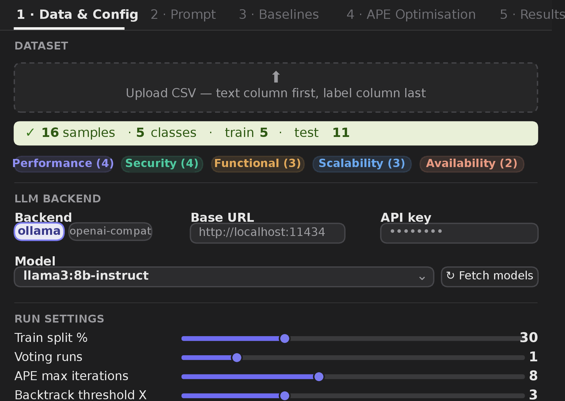
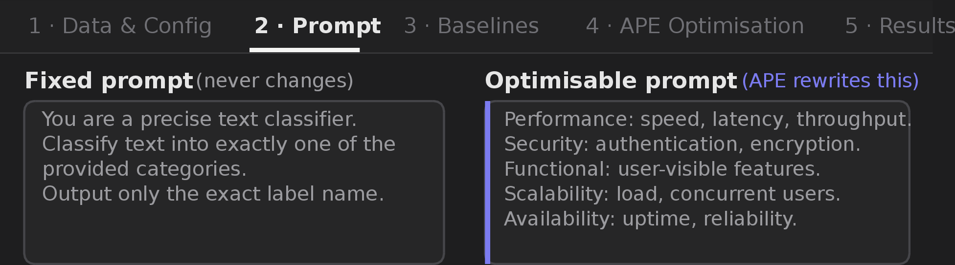
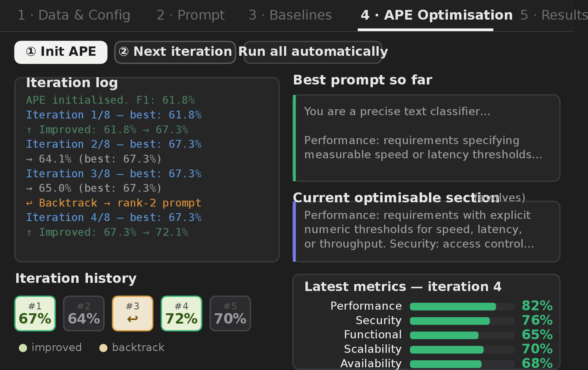
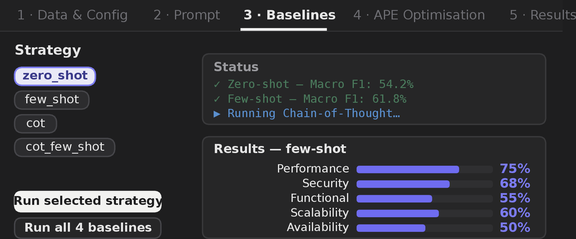
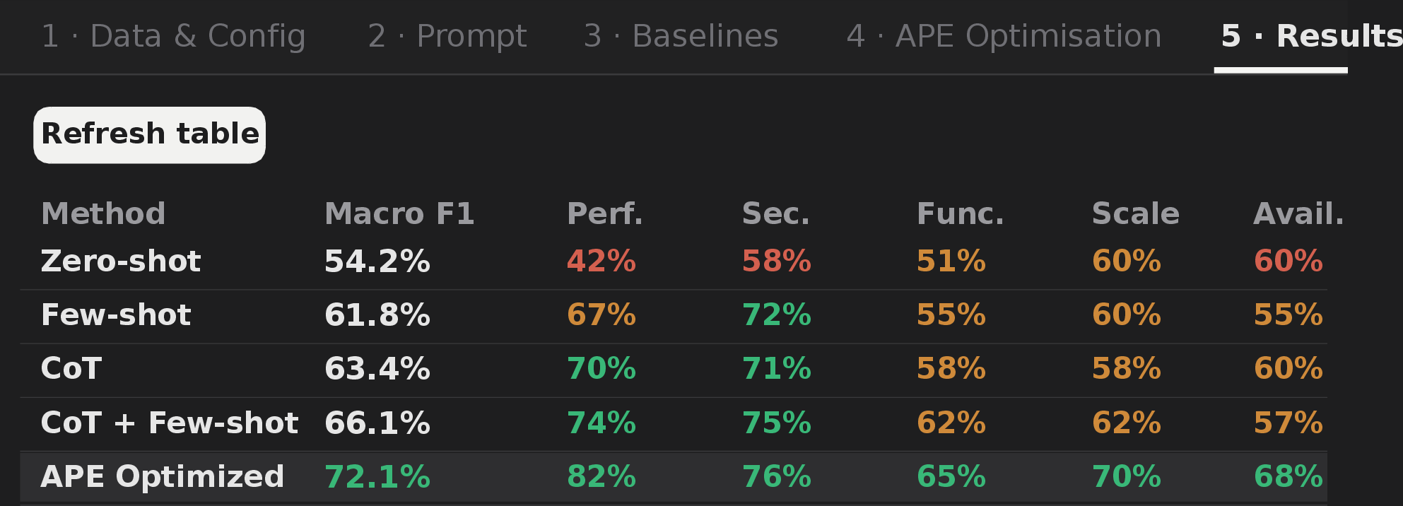
Figure 8: Baselines and Results. (a) Each prompting strategy is run and scored per class. (b) The session summary contrasts the baselines with the BT-APE-optimized prompt; the optimized prompt yields the highest macro F1 and improves the weakest classes.. a — Baselines: per-class F1 per strategy., b — Results: weighted/per-class F1 across methods.
13 Data Leakage Detection in LLMs.↩︎
In the context of requirements classification, data leakage refers to the risk that an LLM has seen parts of the evaluation data during its pre-training, potentially biasing results. A review of the current literature reveals that there is no peer-reviewed paper that systematically addresses this issue. To date, only Zhou et al.[59] has directly investigated data leakage considering that what they have studied different task than the text classification. However, a critical limitation of that work is that the authors assumed prior access to the LLM’s pre-training data, a condition we cannot satisfy. Consequently, we must follow only their core research question, which employed an automated way to study the leakage just based on the behavior of the LLMs. Their experimental results indicate that detecting data leakage using an automated metric like Perplexity is challenging, with accuracy ranging from only 40% to 50% in most cases. They encourage the research community to explore more effective automated methods for identifying data leakage, especially in scenarios where the model’s pre-training data is unknown.
Given this gap, we propose our own approach to study leakage. Specifically, we follow an automated methodology, for measuring similarity between the LLM’s guess and the ground truth, we employ recent similarity metrics such as Jaccard similarity. To evaluate the model’s ability to generate requirement continuations, we first split each requirement into two halves and discard the second half. Let \(n\) be the number of words removed during this trimming step. We then prompt the LLM with the preserved prefix and explicitly instruct it to continue the requirement using approximately \(n\) words. This programmatic constraint ensures that the generated continuation is comparable in length to the original missing segment, allowing us to assess not only semantic coherence but also the model’s ability to reproduce realistic requirement granularity. The results of this analysis will be reported accordingly.
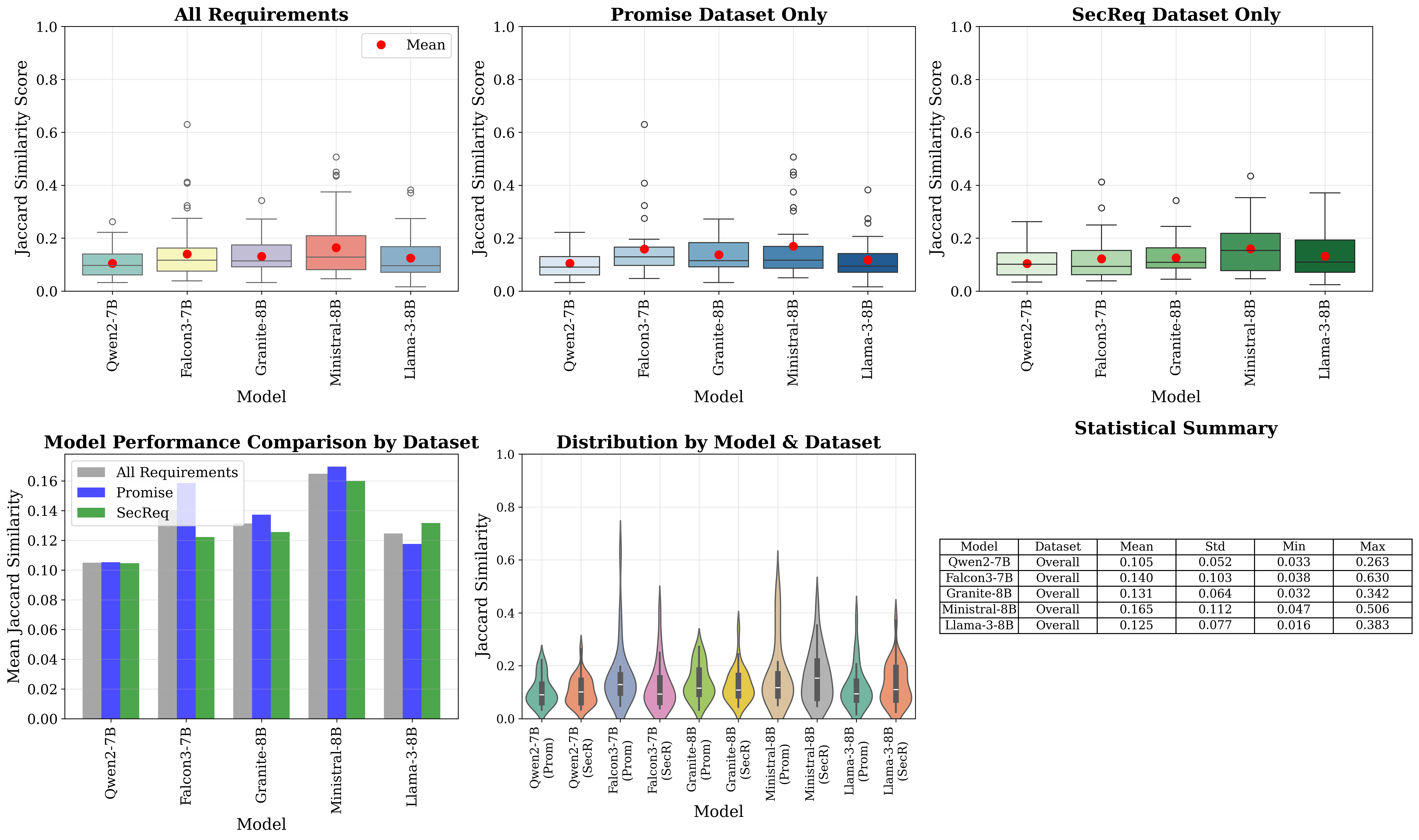
The Jaccard similarity coefficient[60], often denoted as \(J(A,B)\), is a statistic used for comparing the similarity and diversity of sample sets. Defined as the size of the intersection of two sets divided by the size of their union, it quantifies the proportion of shared elements relative to the total distinct elements present in either set. Formally, for two sets \(A\) and \(B\), the Jaccard similarity is calculated as \(J(A,B) = \frac{|A \cap B|}{|A \cup B|}\), where the result ranges from \(0\) (indicating no common elements) to \(1\) (indicating that the two sets are identical). This metric is widely used in fields such as data mining, ecology, and natural language processing, particularly for binary attribute comparison and for measuring the overlap in cluster analysis or document tokenization.
As reported in Figure 9 plots, all observed Jaccard similarities between the predicted trimmed part and the actual trimmed part of the sentence are relatively low. The overall mean scores across all requirements texts range from 0.1048 (Qwen2-7B) to 0.1648 (Ministral-8B), with other models falling in between (Falcon3-7B: 0.1404, Granite-8B: 0.1314, Llama-3-8B: 0.1245). Looking at percentile distributions, most values lie between approximately 0.05 (10th percentile) and 0.25 (90th percentile), depending on the model. For instance, Ministral-8B reaches a 90th percentile of 0.3197 overall, while Qwen2-7B’s 90th percentile is only 0.1779. When comparing datasets, the mean Jaccard scores on Promise (range: 0.1051–0.1695) and SecReq (range: 0.1046–0.1600) are very similar, and t-tests confirm no statistically significant difference between the two datasets for any model (all p-values > 0.17). However, an ANOVA test does indicate significant differences across models (p = 0.0038), suggesting that some models (e.g., Ministral‑8B, Falcon3‑7B) tend to produce slightly higher token overlap than others; given that the residuals follow a normal distribution, the use of ANOVA and T-test are justified.
While these numbers suggest that the models do not strongly reproduce the trimmed second half ground truth — given that Jaccard similarity well below 0.5 indicates limited overlap — we refrain from drawing firm conclusions about the presence or absence of data leakage based solely on this analysis. Several factors could influence these scores, including differences in model output length, tokenization, and inherent generation variability, none of which directly confirm memorization of training data. A more systematic investigation is required to properly separate genuine leakage from other confounding factors. Therefore, we leave a thorough study of data leakage in this context as an item for future work.
14 Prompts and Definitions↩︎
This appendix documents the full set of prompts and class definitions used in our classification experiments, so that the results can be reproduced exactly. We first present the prompt structure: the system prompt that fixes the output format,
followed by the four prompting strategies we compare—zero-shot, few-shot, chain-of-thought (CoT), and chain-of-thought with examples—and the automatic prompt-engineering prompt used to refine the class definitions. The prompt templates are written
generically: the placeholder {classes} is substituted at run time with the list of candidate class labels for the classification task at hand, {class} with a single class label, and {Definitions},
{examples}, and {text} with the corresponding class definitions, in-context examples (few-shot settings only), and the requirement to be classified. We then list the class definitions that are inserted into the
{Definitions} placeholder.
14.1 System Prompt↩︎
As an expert system for classifying software requirements, your task is to carefully analyze each given requirement and assign it to exactly one of the following classes:
{classes}
Output only the label of the class that corresponds to the appropriate class. Do not provide any additional text, definitions, or justification.
14.2 Classification Prompts↩︎
14.2.1 Zero-Shot Prompt (No Examples, No CoT)↩︎
Definitions:
{Definitions}
Requirement: {text}
Using the Definitions above, classify the requirement and provide the final label in the format: "Label: {class}".
14.2.2 Few-Shot Prompt (With Examples, No CoT)↩︎
Definitions:
{Definitions}
Examples:
{examples}
Requirement: {text}
Using the Definitions and Examples above, classify the requirement and provide the final label in the format: "Label: {class}".
14.2.3 Chain-of-Thought (CoT) Prompt (No Examples, With CoT)↩︎
Let’s analyze the classification step by step.
Step 1: Understand the Definitions:
{Definitions}
Step 2: Apply this understanding to classify the following requirement:
Requirement: {text}
Step 3: Provide the final label in the format: "Label: {class}".
14.2.4 Chain-of-Thought with Examples Prompt (With Examples, With CoT)↩︎
Let’s analyze the classification step by step.
Step 1: Understand the Definitions:
{Definitions}
Step 2: Review the Examples:
{examples}
Step 3: Apply this understanding to classify the following requirement:
Requirement: {text}
Step 4: Provide the final label in the format: "Label: {class}".
14.3 APE Prompt↩︎
Role: You are a highly capable, thoughtful, and precise prompt engineer specializing in requirements classification.
Background: A LLM has previously used a set of {Definitions} to automatically classify requirements into the candidate classes {classes}. Based on these definitions, it correctly classified some requirements but misclassified other requirements.
Task: Your task is to enhance the {Definitions} of the classes {classes} to improve the classification accuracy of the large language model. You are given example results in the form [requirement text; true class; predicted class] to guide you in enhancing the definitions.
A set of example requirements that were correctly classified based on the definitions:
{correctly_classified}A set of example requirements that were incorrectly classified based on the definitions:
{misclassified}
You may add content, shorten, or rephrase the definitions to improve clarity and accuracy.
Let’s think step by step:
Study the Definitions: Understand the provided definitions of the classes.
Analyse Examples: Analyze correctly classified and misclassified examples.
Success analysis: For each correctly classified example identify why the original definitions were successful. Ask yourself: Do certain words/phrases consistently lead to correct classification? Which parts of the definitions are clear, complete, and unambiguous?
Error analysis: For each misclassified example identify why the original definitions failed. Ask yourself: Do certain words/phrases consistently mislead? Are the definitions ambiguous, incomplete, or overlapping?
Enhance Definitions: Enhance the definitions by adding, reducing, or rephrasing content.
Enhancement Procedure: For problematic classes:
Add discriminative features: Incorporate missing characteristics from misclassified examples.
Create exclusion clauses: Explicitly state what doesn’t qualify (“This class excludes…”).
Use comparative framing: Highlight differences between easily confused classes.
Simplify if needed: Simplify definitions when they appear to be too complex.
Rephrase if needed: Rephrase definitions when the phrasing or terminology is misleading.
Validation Constraints:
Ensure misclassification prevention: The revised definitions must theoretically prevent the same errors from recurring.
Avoid overfitting: Definitions should maintain generalizability through clear principles rather than example-specific fixes.
Output the enhanced {Definitions} only, with no additional text.
14.4 Class Definitions↩︎
These are the definitions inserted into the {Definitions} placeholder of the prompts above.
14.4.0.1 Security Requirements.
Security requirements are prescriptive constraints imposed on a system’s functional behaviour to operationalise its security goals. They are not functional requirements themselves but restrict how functions are performed in order to prevent, detect, or recover from harm, and are expressed in precise, operational terms that are clear enough for implementation by system designers and architects. Security requirements are derived from business and functional goals and may be categorised as primary—those derived directly from business and functional goals, whose satisfaction ensures the system meets its fundamental security objectives—or secondary—those that support the implementation of primary requirements (e.g.through detection or recovery) when direct enforcement is infeasible or too costly. They are manifestations of high-level organisational policies into the detailed requirements of a specific system and are deeply tied to the broader system context, which may extend beyond software to include other components or processes. Security requirements specify the system’s security policies and must address risks, threats, and assets, while influencing and being influenced by security mechanisms, vulnerabilities, and attacks.
14.4.0.2 Non-Security Requirements.
Non-security requirements are constraints or specifications that govern a system’s behaviour, performance, and structure without being directly tied to security goals. Unlike security requirements, they do not aim to prevent, detect, or recover from harm, and do not operationalise security policies. They may include functional requirements (which define what the system should do) and other non-functional requirements such as performance, usability, reliability, scalability, and maintainability. Non-security requirements are typically derived from business needs and user expectations but are not intended to address risks, threats, or vulnerabilities. While they may influence system design and operation, they do not explicitly enforce security mechanisms or aim to mitigate security concerns.
14.4.0.3 Functional Requirements.
Functional requirements define the essential functions a system must perform, the services it must offer, and the behaviours it must exhibit under specified conditions. They focus on what the system should do—describing actions, operations, or transformations the system executes—without addressing implementation constraints. They typically specify the inputs (stimuli) to the system, the outputs (responses) from the system, and the behavioural relationships between them. In practice, they outline the specific behaviours, features, and capabilities the system must have to meet user needs and achieve its intended purpose, such as user authentication, data storage, report generation, or integration with other systems.
14.4.0.4 Non-Functional Requirements.
Non-functional requirements do not define the essential functions a system must perform, the services it must offer, or the behaviours it must exhibit under specified conditions. They do not focus on what the system should do—avoiding descriptions of actions, operations, or transformations the system executes—and instead address implementation constraints. They typically exclude specifications of inputs (stimuli) to the system, outputs (responses) from the system, and behavioural relationships between them. They encompass a system’s quality-related attributes as well as the constraints under which the system must operate—for example performance, scalability, portability, compatibility, reliability, maintainability, availability, security, and usability—specifying how a system should behave rather than what it should do.
14.4.0.5 Quality Requirements.
A quality requirement expresses how well a system or service should execute an intended function. Quality requirements include attributes or constraints that address product-quality aspects and quality-in-use aspects. Product-quality aspects include functional suitability, reliability, performance, efficiency, usability, maintainability, security, compatibility, and portability. Quality-in-use aspects include satisfaction, effectiveness, freedom from risk, efficiency, and context coverage. Quality requirements often address the global properties or characteristics of the system rather than those of specific functions.
14.4.0.6 Non-Quality Requirements.
A non-quality requirement does not express how well a system or service should execute an intended function. Non-quality requirements exclude attributes or constraints that address product-quality and quality-in-use aspects. They do not include the product-quality aspects of functional suitability, reliability, performance, efficiency, usability, maintainability, security, compatibility, or portability; nor the quality-in-use aspects of satisfaction, effectiveness, freedom from risk, efficiency, or context coverage. Non-quality requirements do not typically address the global properties or characteristics of the system; instead, they focus solely on the properties of specific functions.
References↩︎
https://huggingface.co/spaces/open-llm-leaderboard/open_llm_leaderboard↩︎
Notation for hypotheses. Throughout Sections 4.4–4.7, we denote hypotheses using \(H^{\text{RQ}n}_{k,0}\) for the null and \(H^{\text{RQ}n}_{k,A}\) for the alternative, where \(n\) is the research question and \(k\) indexes the hypothesis within that question. For example, \(H^{\text{RQ}1}_{1,0}\) is the first null hypothesis under RQ1 and \(H^{\text{RQ}2}_{2,A}\) the second alternative hypothesis under RQ2.↩︎
The tool’s interface is built with Gradio https://www.gradio.app; dataset handling and metric computation use pandas https://pandas.pydata.org and scikit-learn https://scikit-learn.org; model inference is issued through the requests HTTP client https://requests.readthedocs.io to an Ollama https://ollama.com (or OpenAI-compatible) backend.↩︎