A Simple Solution to Improving Human Supervision of Algorithms: Evidence from Smart Vending
July 01, 2026
1 Introduction↩︎
Data-driven decision-making is transforming businesses by automating complex and frequent tasks previously reliant on human judgment [1], [2]. Algorithms and artificial intelligence (AI) systems are now routinely employed in critical decision-making domains such as drug discovery [3] and digital content recommendation [4]. Despite substantial advancements in algorithmic capabilities, many organizations continue to grant frontline employees discretionary power to override algorithmic recommendations. Such override rights reflect a widespread managerial belief that human workers possess contextual or local information unavailable to algorithms, which can potentially enhance decisions when algorithms falter.
However, the causal impact of human overrides on algorithmic performance remains ambiguous. While a considerable body of literature (e.g., [5]–[7]) indicates that human overrides can degrade the performance of autonomous algorithmic decisions, highlighting the risks of human bias, there is also evidence suggesting that overrides can sometimes improve outcomes. For example, overrides have been shown to be beneficial when humans utilize domain-specific insights not captured by the algorithm [8], [9]. Thus, despite significant advancements in automation, human operators can still possess critical private information that enhances the quality of decision-making. These mixed findings raise an essential design question: How should override rights be structured to improve human-AI collaboration when AI systems operate autonomously?
This question defines an important regime in human-AI collaboration, where autonomous systems make routine decisions while human supervisors primarily execute and occasionally intervene through discretionary overrides. This setup is increasingly common in operational contexts such as retail, logistics, and resource planning, where AI handles frequent, moderate-stakes tasks and humans step in selectively. In these settings, neither humans nor algorithms consistently outperform the other; effectiveness depends on the nature of the decision [10], the allocation of authority [11], and how discretion is structured within the organization [12]. Despite its practical relevance, the design of override rights, specifying who may intervene, under what conditions, and to what extent, remains theoretically underdeveloped and lacks empirical guidance. This contrasts with a different regime in which AI serves as an assistant: algorithms provide input, but humans make the final decision in every case. It emerges more commonly in high-stakes domains such as loan approvals [9], [13] or medical diagnosis [14], [15]. Recent research has explored how algorithm design and presentation improve outcomes by enhancing user trust through modifiable outputs [16], tailoring advice to expert needs [17], prompting reflective judgment via diagnostic support [18], and mitigating trust-eroding bias amplification in feedback loops [19].
Designing effective override policies for autonomous AI systems raises two distinct challenges. First, override decisions are inherently endogenous. Evaluating their effectiveness requires a counterfactual comparison between the actual override and the algorithm’s original recommendation, yet only one of these is observed. As a result, causal assessment typically relies on randomized experiments that induce exogenous variation in override behavior [6], [20] or on imputation using observational data [5], [9], which is more tractable when the outcome variables are binary. Second, override discretion is difficult to manage precisely because it is internal: workers must judge when intervention is warranted, despite cognitive limits [21], biased self-assessment [22], and limited feedback [23]. These constraints make it difficult to assess, influence, or improve discretionary behavior directly.
In this paper, we address these challenges and show that the causal value of human overrides depends critically on the structure of discretion. We introduce a constrained override policy that limits the number of overrides workers can make per decision episode. This simple cardinality constraint does not improve judgment per se, nor does it require identifying useful overrides in advance. Instead, it changes the decision environment: when override opportunities are scarce, workers are forced to prioritize. We term this the selective filtering mechanism, a process that screens out noisy overrides while preserving those with stronger private information. By converting unconstrained discretion into a filtering task, the policy transforms noise-prone override behavior into a scalable and effective mechanism for improving human-algorithm collaboration.
Our study is motivated by a collaboration with Fengyi Technology, one of the largest smart vending machine retailers in China. By the end of July \(2025\), the company operated over \(170,000\) smart vending machines across major cities. Each day, Fengyi uses centralized machine learning algorithms to generate replenishment recommendations, specifying the quantity of each stock-keeping unit (SKU) for every machine in the network. These decisions are executed by local workers, each responsible for replenishing \(80\)-\(100\) machines using inventory from nearby warehouses. Workers are expected to follow algorithmic suggestions but retain discretion to increase stock for SKUs they expect to sell out.
A key concern arises around downward overrides, instances where workers reduce the algorithm’s suggested quantity. In a \(2022\) pilot study, Fengyi found that granting unrestricted override rights led to a measurable decline in sales, despite workers’ incentives being aligned with both sales and inventory efficiency. That is, workers receive bonuses for achieving high sales but face penalties for excess inventory that remains unsold. At the same time, firm managers acknowledged that workers often possess valuable local information, such as customer preferences, store-level events, or nearby competition, that the algorithm cannot observe. This creates a core operational dilemma: how to preserve the benefits of human overrides while mitigating the risks of performance loss. The company sought a scalable policy that could structure discretionary power to better filter high-value human overrides.
To formalize our proposed solution, we develop a stylized Bayesian model [24], [25] in which workers receive private signals about the potential benefit of overriding each SKU. These signals are both noisy and biased, reflecting imperfect human judgment. Under a free override policy, workers act on all signals exceeding a subjective threshold, resulting in a mix of low- and high-quality decisions. A constrained override policy, by limiting the number of allowable overrides, induces endogenous selection based on signal strength: workers are forced to rank-order override opportunities and act only on the most compelling ones. This selective filtering process raises the average quality of overrides without requiring the ex-ante identification of useful cases.
While not intended as a comprehensive model of human behavior, our framework serves to illustrate the selective filtering hypothesis. The idea that structural constraints can improve decision quality is well-established. Prior work has shown that limiting options or reducing cognitive load can enhance performance, whether through choice set simplification [26], [27] or cognitive bandwidth constraints [28]–[30]. We demonstrate that these classical insights also apply to human supervision of algorithms, where a simple cardinality constraint transforms override discretion into a prioritization task. To establish the robustness of this mechanism, we further develop a rational inattention formulation [31], [32], in which workers further endogenize a cost for information acquisition in decision-making. Both formulations yield the same core logic: constraints filter noise by concentrating attention on the most valuable overrides. These results suggest that while different behavioral models offer plausible microfoundations, the effectiveness of constrained override does not depend on the specific structure of human decision-making.
Guided by the theoretical prediction, we designed a randomized field experiment involving \(553\) workers managing over \(59,000\) vending machines and approximately \(4,000\) SKUs. Workers were randomly assigned to one of three override policies that differed only in the extent of downward discretion: (1) no override, which prohibited reductions to algorithmic recommendations; (2) free override, which permitted unrestricted reductions; and (3) constrained override, which limited each worker to reducing at most two SKUs per machine. All groups retained full discretion to increase replenishment quantities, and in rare cases, such as warehouse stockouts, additional reductions were allowed for all groups. A key feature of our design is that randomization occurs at the worker level. This departs from prior studies that randomize at the SKU or decision level [6], [7], which fix override opportunities and thus preclude endogenous prioritization. In contrast, our design allows workers to allocate discretion across SKUs, enabling us to test whether constrained override induces workers to prioritize their strongest override signals, a central implication of the selective filtering mechanism.
We estimate the causal effects of override policies using a worker-machine-day panel and a difference-in-differences specification, comparing the constrained and free override groups to the no-override baseline. We measure performance outcomes at the machine level based on SKU-level sales and inventory between consecutive replenishments. The free override policy reduces inventory by \(1.95\%\) (\(p<0.01\)) but also lowers daily sales by \(1.19\%\) and sales probability by \(1.38\) percentage points (\(p<0.01\)). The negative impact of unconstrained discretion aligns with prior work showing that unstructured human overrides can degrade algorithmic performance [6], [7], [9]. In contrast, constrained override reduces inventory by \(1.28\%\) (\(p<0.01\)) without affecting sales quantity or probability, suggesting more selective and effective override behavior. These results are robust to alternative scalings and demand irregularities, reinforcing the conclusion that override policy shapes override quality.
We then examine how override policies directly influence worker behavior. The free override policy leads to broad-based reductions: workers replenish fewer SKUs (\(-0.55\), \(p < 0.01\)), lower total quantities (\(-3.82\), \(p < 0.01\)), and apply smaller reductions per SKU (\(0.12\)). The constrained override policy, in contrast, narrows the scope of overrides: workers override significantly fewer SKUs (\(0.36\) vs.\(1.96\), \(p < 0.01\)), but implement larger reductions per SKU (\(0.75\), \(p < 0.01\)). While upward overrides increase modestly, the changes are insufficient to offset the focused nature of constrained downward overrides. The evidence indicates a more selective pattern of overrides: the constrained override policy reduces the frequency of overrides and refocuses discretion on a smaller set of high-confidence decisions.
To directly test the selective filtering mechanism, we adopt a local average treatment effect (LATE) framework [33], using randomized override policy assignment as an instrument for SKU-level override decisions. The LATE precisely captures the causal effect of override decisions for the subset of SKUs whose status is altered by the policy. Comparing the constrained override policy to the no override policy, we estimate a LATE of \(-3.45\) items in inventory (\(p < 0.01\)), with no significant change in sales quantity or probability, evidence of precise inventory reductions. In contrast, the free override policy yields smaller inventory reductions (\(-1.26\)) but significantly decreases the probability of sale by \(10.55\) percentage points (\(p < 0.01\)), indicating that unconstrained discretion results in lower-quality overrides. Robustness checks further reinforce this mechanism: intent-to-treat estimates show a consistent directionality; stricter definitions of override (e.g., zeroing out SKUs) yield larger LATEs; upward overrides exhibit no significant effects; and constrained LATE estimates remain stable after controlling for SKU features such as price and discount status.
To translate the mechanism into practice, we examine when constrained overrides are most effective. We focus on three dimensions where the value of human discretion is likely to vary: worker experience, SKU-level incentive alignment, and algorithmic uncertainty. The constrained override policy yields the largest performance gains among senior workers, who reduce inventory by \(1.72\%\) (\(p < 0.01\)), and for growth-stage SKUs, where inventory declines by \(1.15\%\) (\(p < 0.05\)) without reducing sales. It also performs well for top-selling SKUs, reducing inventory by \(1.9\%\) (\(p < 0.01\)); these products are more tied to compensation, aligning worker incentives with performance. In contrast, the free override policy reduces sales by \(1.39\%\) and inventory by \(2.85\%\) among senior workers (\(p < 0.01\)) and increases inventory for low-sales SKUs (\(+1.16\%\), \(p < 0.1\)) while depressing sales across the board. These patterns suggest that the constrained override policy is most beneficial when workers possess stronger private signals, are more incentive-aligned, or when algorithmic forecasts are less reliable. At the same time, the consistent performance losses under the free override policy indicate that full discretion amplifies noise, even among experienced workers and high-value SKUs.
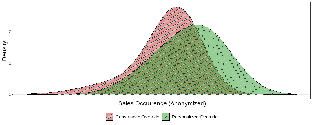
Finally, we develop a data-driven refinement that adaptively filters human overrides at the instance level. Using override decisions from the constrained group as a behavioral benchmark, we train a logistic regression model to estimate the likelihood that a given override reflects high-quality private information. This model is then used to simulate a personalized policy: override instances from the free group are accepted if their predicted probability exceeds a threshold and are rejected otherwise. The resulting personalized override group exhibits a heavier tail in override volume per machine and a significantly higher sales probability, an increase of \(9.1\) percentage points (\(p < 0.01\)) compared to the original constrained group.
Before proceeding, we summarize our main contributions in three aspects:
We propose a simple override policy, constrained override, for the regime of autonomous AI with human supervision to improve human-AI collaboration. By imposing a cardinality constraint, the policy activates a selective filtering mechanism that transforms override discretion into a prioritization task, filtering noise and surfacing high-value human input. While classical behavioral models offer plausible microfoundations, the effectiveness of the constrained override policy does not depend on the specific structure of human decision-making.
We provide causal evidence on override policies through a randomized field experiment. While the free override policy reduces both inventory and sales, consistent with prior findings on the risks of unstructured human discretion, the constrained override policy reverses this pattern, improving inventory efficiency without reducing sales. A local average treatment effect framework confirms that these gains reflect improved override precision, offering causal support for the selective filtering mechanism.
We demonstrate that the constrained override policy is a scalable, low-cost intervention for improving human supervision of autonomous AI. It requires no algorithm redesign, no information customization, and no identification of private signals. The approach is easy to implement, generalizes across operational contexts, and enables firms to enhance decision quality without added complexity.
The rest of the paper is structured as follows: Section 2 reviews related literature; Section 3 describes the empirical context, key hypotheses, and experimental design; Section 4 estimates the causal effects of override policies on performance and behavior; Section 5 tests the proposed mechanism; and Section 6 offers practical guidance through heterogeneous effects.
2 Literature Review↩︎
Prior research offers mixed evidence on the performance implications of human overrides to algorithmic recommendations. A substantial body of work finds that discretionary overrides degrade outcomes: manual price changes reduce revenue [7], [34], task reassignments lower productivity [5], and forecast revisions increase error rates [35]. Experimental studies similarly show that override discretion introduces inconsistency and noise [36], [37], motivating calls for strict algorithm adherence [38], [39]. In contrast, other work finds that override discretion can improve performance when humans possess relevant private information. For example, [6] shows that workers improve inventory decisions for growth-stage SKUs, while [23], [8] and [9] find that forecasters enhance accuracy by addressing algorithmic blind spots. [40], [41], and [42] further demonstrate that targeted overrides can correct systematic algorithmic errors. We reconcile these findings by showing that override effectiveness depends not on frequency but on the structure of discretion. Using field-based causal evidence, we demonstrate that a constrained override policy improves decision quality by inducing prioritization, whereas unconstrained discretion amplifies noise.
Behavioral research offers foundational insight into why override discretion often leads to suboptimal outcomes. Bounded rationality and overconfidence are well-documented sources of systematic error [43]–[45], and persistent deviations from optimality have been observed in inventory and transshipment contexts due to biased self-assessment and miscalibrated expectations [46]–[48]. These effects are amplified by limited feedback and misaligned incentives [49]–[51]. Override behavior is also shaped by cognitive constraints: [21] finds that humans often misjudge whether to delegate to algorithms, even when algorithmic outputs are demonstrably more accurate. Related studies show that decision quality deteriorates when individuals face excessive choice [26], operate under time pressure [28], or must allocate limited attention across competing alternatives [29], [30]. Algorithm aversion further reduces override effectiveness: individuals penalize machine errors more heavily than human ones [52], and override behavior is shaped by perceived control and transparency [16], [53]. Additional frictions stem from empathy gaps [54], social influence [55], and subjective overreliance [22]. Building on this foundation, our contribution is to show that structural constraints can improve override quality by reshaping discretion in ways that align with these behavioral limits. Unlike prior work that seeks to suppress overrides or correct judgment directly, we offer a design-based solution that accommodates multiple behavioral microfoundations, such as Bayesian learning or rational inattention, without relying on any specific cognitive model.
Recent work has begun to examine when override discretion adds value. Most approaches follow a two-stage logic: they first detect cases where human overrides improve outcomes and then modify algorithmic or organizational responses accordingly. For example, [6] identify product categories where overrides improve inventory efficiency, while [20] develop adaptive systems that respond to human-identified product features. Similarly, [41] and [40] show that override value increases when algorithmic errors are predictable. These solutions rely on behavioral modeling, domain-specific detection, or retrospective validation, making them difficult to scale across settings. In contrast, we offer a structural solution that induces prioritization at the point of discretion. Without requiring behavioral labels or predictive models, our approach filters high-value overrides through a simple constraint that reallocates attention across competing options.
A complementary body of work examines how to structure human-AI collaboration in ways that preserve human judgment while ensuring algorithmic consistency. Comparative studies in knowledge work, such as editorial decisions, reveal systematic advantages and limitations on both sides [56]. In high-stakes domains like healthcare and finance, algorithms serve as advisors, while humans retain decision authority. Research in this regime focuses on interface design, transparency, and explanation quality to improve adherence and performance [13], [15], [57]–[59]. In contrast, many operational settings, including ours, assign decision rights to autonomous systems, with humans intervening only occasionally through override discretion. Work in this context has explored override shaping through forced prompts [60], learned delegation rules [61], and hybrid control frameworks that incorporate human input into algorithmic models [62]–[64]. Others investigate whether explanation design improves override quality [65]. While these approaches are promising, they often depend on dynamic learning systems, behavioral personalization, or interface-level engineering. We offer a lightweight alternative without modifying the algorithm or customizing the interface.
3 Research Context, Theoretical Rationale, and Experiment Design↩︎
We first describe Fengyi Technology’s business setting regarding smart vending machines. Next, we introduce our proposed solution and outline the hypothesis. Finally, we design a randomized field experiment to evaluate its effectiveness.
3.1 Empirical Context↩︎
Fengyi Technology is a leading self-service retail operator in China specializing in smart vending machines. As of July \(2025\), the company’s service network spanned more than \(70\) metropolitan areas, managed approximately \(170,000\) machines, and served over \(75\) million consumers nationwide. Each vending machine offers ready-to-consume products such as breakfast items, snacks, dairy, and beverages, with typical assortments ranging from \(40\) to \(50\) SKUs. These machines are deployed in diverse offline environments such as office buildings, hotel lobbies, and outdoor public areas (see also Figure 3 in 8.1 of the online appendix). All machines are connected to a centralized server via the internet, enabling real-time data collection and system-wide algorithmic management. This infrastructure allows the firm to dynamically forecast demand, monitor sales, and remotely update replenishment recommendations on a daily basis.
A core operational task at Fengyi Technology is inventory replenishment, carried out by a large network of local workers. Each worker restocks \(80\) to \(100\) machines and typically services \(10\) to \(15\) per day using inventory from a nearby warehouse. To support this process, the company runs a centralized algorithm that provides daily SKU-level replenishment recommendations for each machine. These recommendations are derived from a two-stage system: a machine learning model first forecasts product-level demand based on historical sales, current inventory, and contextual features (e.g., day of week, weather, location type), and then a replenishment policy optimizes the replenishment quantity based on those forecasts. The algorithm follows a standard periodic review structure, specifically, an \((R, T)\) policy [66], which determines restocking quantities by topping inventory back up to a target level \(R\) every \(T\) days. While the specific details of the forecasting and control models are not the focus of this study, they remained fixed throughout our experiment to provide a consistent baseline. A mobile app delivers recommendations that show, for each SKU on each machine, the recommended replenishment quantity, for example, “place \(5\) cans of Coke on Machine A\(124\)." The app also displays supporting information such as current inventory levels, historical daily sales, and warehouse stock availability, enabling workers to interpret and potentially override the suggestions in the field. (Please also refer to 5 in the online appendix 8 for screenshots of the app interface.)
The company manages a performance-based incentive system that evaluates workers based on both sales and inventory. Workers receive bonuses for achieving high sales but face penalties for excess inventory that remains unsold. Therefore, stocking more increases the chance of capturing demand but also raises the risk of spoilage or overstock penalties, especially for slow-moving or perishable items. Incentivized by bonuses and penalties, workers may override the algorithmic suggestion when they believe the algorithm falls short. Based on anecdotal evidence, some workers develop informal relationships with consumers and gain insights into product preferences that are not recorded in data. In addition, workers are sensitive to nearby competition, such as the presence of a convenience store offering discounts on similar items, which can influence demand in ways the centralized system does not capture [67].
To test whether private, context-specific knowledge could improve replenishment performance, Fengyi Technology conducted a small-scale pilot in early \(2022\). In this trial, selected workers operated under a free override policy that allowed them to override algorithm-suggested replenishment quantities without restrictions. The intervention led to a decline in overall sales, primarily due to widespread lost sales across SKUs caused by excessive downward overrides. These findings suggest that although workers may possess valuable private information, a free override policy can also introduce substantial noise and compromise performance. In response, the company applied a no (downward) override policy that prohibited workers from reducing the algorithm’s suggested replenishment quantity for any SKU but retained full discretion to increase it. Accordingly, workers are instructed to treat the algorithm’s recommendation as a minimum threshold, except in rare cases such as warehouse shortages. For example, if the system recommends restocking \(10\) units of bottled milk but only \(6\) are available at the warehouse, the worker may reduce the replenishment quantity to match available stock.
3.2 Solution and Key Hypothesis↩︎
To address the limitations of both the no override and free override regimes, we propose a simple policy: constrained override. This policy imposes a cardinality constraint that limits each worker to overriding at most \(K\) SKUs per machine. As illustrated in Figure 1, varying levels of discretion lead to different override behavior and consequences. Under all policies, workers may still override in extreme cases (e.g., warehouse stockouts). The no override policy provides no discretionary power beyond such exceptions. The free override policy grants full discretion, resulting in a mix of “good” overrides (which reduce inventory without harming sales) and “bad” overrides (which lead to lost sales). Positioned in between, the constrained override does not simply yield a random subset of \(K\) overrides from the free override case, as workers are incentivized to improve inventory efficiency. Instead, by limiting the number of allowable downward overrides, the constrained policy motivates selective filtering: workers prioritize SKUs where they are more confident in their judgment. This “sorting effect" increases the proportion of”good" overrides.
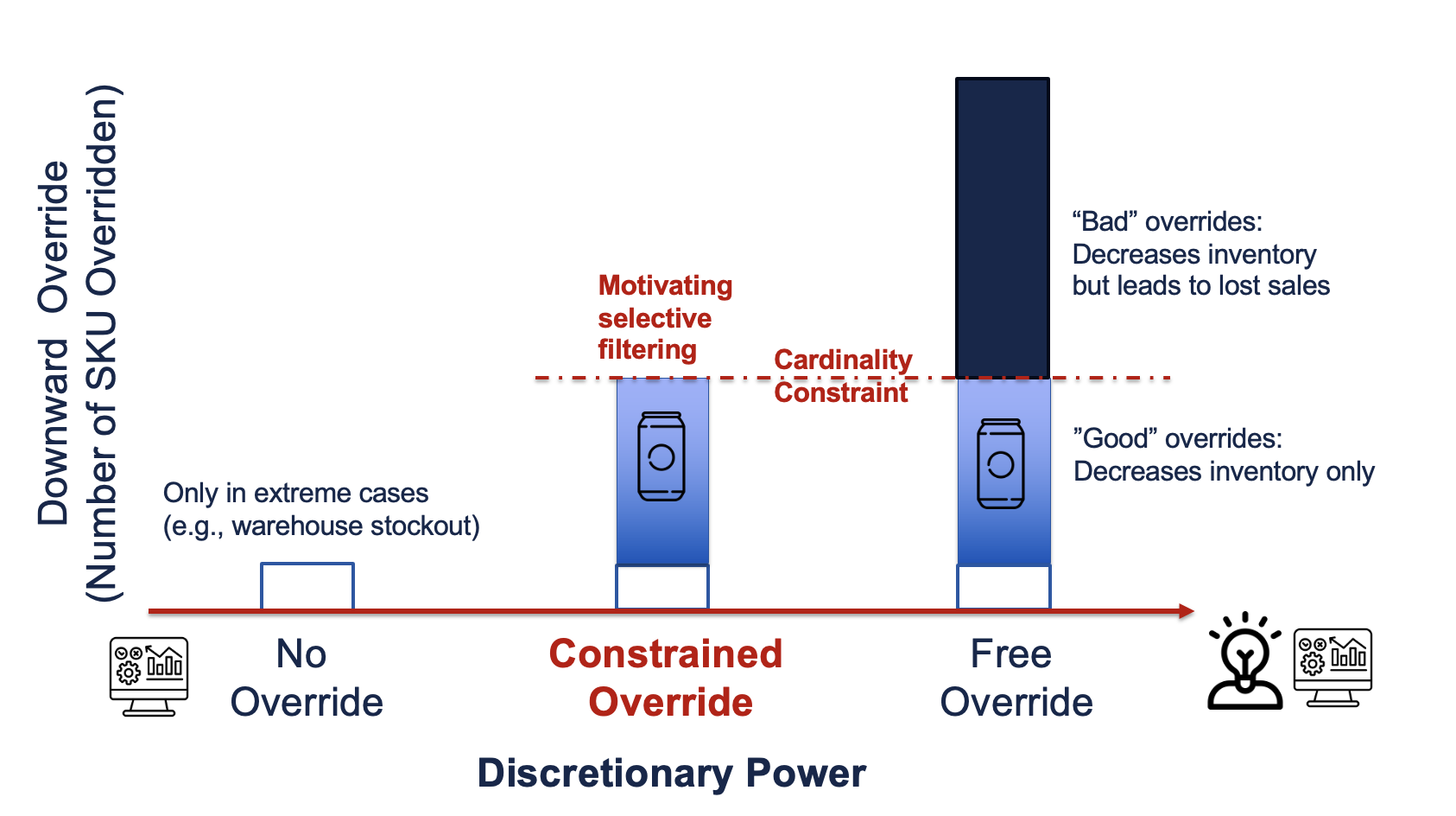
To formalize this intuition, we develop a stylized Bayesian model in which workers select which SKUs to override based on noisy private signals and estimation bias. The model clarifies how a cardinality constraint induces a sorting effect, where workers prioritize SKUs with stronger signals. This mirrors classic results in signal-based screening and statistical discrimination [24], [25], where decisions based on noisy signals can still improve aggregate outcomes.
Specifically, we consider a single decision episode when replenishing a machine stocked with \(N\) SKUs, indexed by \(k = 1, \dots, N\). Replenishment occurs for all SKUs based on the algorithm’s suggestions, yielding a baseline performance outcome \(v_k^s\) for each SKU \(k\), observable to both the firm and the worker. If the worker overrides by reducing the algorithm’s suggested replenishment level for a selected SKU \(k\), the actual performance becomes \(v_k^a = v_k^s + \eta_k\), where \(\eta_k \sim \mathcal{N}(\mu, \sigma_\eta^2)\) with \(\mu < 0\) representing SKU-specific local knowledge available only to the worker, such as nearby competition or contextual factors not captured by the algorithm. Here, we can also think of \(\eta_k\) as the individual causal effect of override. A positive \(\eta_k\) indicates a “good" override (private information), while a negative \(\eta_k\) indicates a”bad" override (human bias). The overall performance across all SKUs is thus \(\sum_{k=1}^N v_k^a = \sum_{k=1}^N v_k^s + \sum_{k \in A} \eta_k\), where \(A\) is the set of overridden SKUs. The true distribution reflects a mild negative bias (\(\mu < 0\)), consistent with empirical evidence that humans often naively overweight noisy private signals, leading to a systematic negative impact of overrides [6].
The worker does not observe \(\eta_k\) directly but instead receives a noisy private signal \(s_k = \eta_k + \epsilon_k\), where \(\epsilon_k \sim \mathcal{N}(0, \sigma^2)\) represents independent judgment noise. We assume that workers believe \(\eta_k \sim \mathcal{N}(0, \sigma_\eta^2)\), reflecting potential miscalibration in perceiving the value of their local knowledge. We further assume that \(\eta_k\) and \(\epsilon_k\) are independent across SKUs. The worker uses \(s_k\) as a noisy proxy for the override’s value and makes decisions accordingly. Each time a worker replenishes a machine, they choose a subset \(A \subseteq \{1, \dots, N\}\) of SKUs to override to maximize the expected cumulative value of override, \(\sum_{k \in A} \mathbb{E}[\eta_k \mid s_k]\), subject to a policy-specific constraint on \(A\). Thus, the override decision is fully endogenized: the worker selects SKUs based on Bayesian inference and under different override policies.
The additive signal structure and normality assumptions are standard in Bayesian models of noisy information (e.g., [25]). We assume aligned incentives: workers override to improve performance, consistent with compensation and penalties tied to sales and inventory (Section 3.1). These simplifications help isolate the core mechanism, how override policy shapes the interaction between local knowledge (\(\eta_k\)) and judgment noise (\(\epsilon_k\)). Our setup also parallels classic delegation models (e.g., [68], [69]), but shifts focus from incentive misalignment to selective filtering under noise.
No Override Policy: The worker follows all algorithmic suggestions without exceptions. Since neither local knowledge (\(\eta_k\)) nor judgment noise (\(\epsilon_k\)) is used, this policy eliminates human error but also ignores potential benefits from local knowledge. Therefore, the override set is \(A^{\text{No}} = \emptyset\).
Free Override Policy: The worker may override any SKU based on the perceived signal \(s_k = \eta_k + \epsilon_k\). Given the miscalibration of workers’ prior belief \(\eta_k \sim \mathcal{N}(0, \sigma_\eta^2)\), the posterior expectation is \(\mathbb{E}[\eta_k \mid s_k] = \frac{\sigma_\eta^2}{\sigma_\eta^2 + \sigma^2}s_k\). Then, the worker’s override set is \(A^{\text{Free}} = \{k: s_k > 0\}\).
Constrained Override Policy: The worker maximizes the expected override value by selecting the top \(K\) SKUs with the highest signals among the set \(\{k: s_k > 0\}\), since the posterior expectation \(\mathbb{E}[\eta_k \mid s_k]\) increases strictly in \(s_k\). Formally, the override set is \(A^{\text{Constrained}} = \{k: s_k > 0, s_k \ge s_{(K)}\}\), where \(s_{(1)} \ge s_{(2)} \ge \dots \ge s_{(N)}\) are the ordered signals. To simplify analytical derivations, we approximate \(A^{\text{Constrained}} \approx \{k: s_k \ge s_{(K)}\}\) by dropping the threshold \(s_k > 0\) with a negligible approximation error when \(K \ll N\).
Lemma 1 (Selective Filtering Mechanism of Private Information). For any SKU \(k\in[N]\), the expected override value conditional on being selected under the constrained override policy is strictly positive if the following condition holds: \[\mathbb{E} \left[ \eta_k \mid k \in A^{\text{Constrained}} \right] > 0 \quad \text{if} \quad a(K) > -\mu \cdot \frac{\tau}{\sigma_\eta^2}.\] Here \(\tau^2 \mathrel{\vcenter{:}}= \sigma_\eta^2 + \sigma^2\) and \(a(K) \mathrel{\vcenter{:}}= \frac{1}{K} \sum_{j = 1}^{K} \mathbb{E}\left[U_{(j)}\right]\), with \(U_{(1)} \ge U_{(2)} \ge \dots\ge U_{(N)}\) representing the order statistics of \(\{U_1, \dots, U_N\}\), defined by \(U_k \mathrel{\vcenter{:}}= (s_k - \mu)/\tau\).
We place all proofs in the online appendix (8.2). Intuitively, 1 shows that when the override constraint is imposed, workers focus on SKUs with the strongest signals. Since \(s_k\) is positively correlated with \(\eta_k\) by definition, this sorting raises the expected value of selected overrides, as long as \(K\) is sufficiently small (or equivalently, \(a(K)\) sufficiently large). We now formally compare informational efficiency across policies by aggregating \(\eta_k\) in the selected sets.
The total expected override values across the three override policies satisfy: \[\mathbb{E}\left[\sum_{k \in A^{\text{Constrained}}} \eta_k \right] > \mathbb{E}\left[\sum_{k \in A^{\text{No}}} \eta_k \right] = 0 > \mathbb{E}\left[\sum_{k \in A^{\text{Free}}} \eta_k \right]\] if the model parameters satisfy \(h\left( -\mu / \tau \right) < -\mu \cdot \tau / \sigma_\eta^2 < a(K),\) where \(h(x) \mathrel{\vcenter{:}}= \frac{\phi(x)}{1-\Phi(x)}\), and \(\phi\), \(\Phi\) denote the standard normal probability density function (PDF) and cumulative distribution function (CDF), respectively.
Our theoretical model is not a comprehensive account of human decision-making, but a stylized framework to clarify the logic behind our empirical hypothesis (i.e., selective filtering). The idea that constraints (in various forms) improve decision-making is not new. There are several classical works on how structural and cognitive limits shape behavior, including studies on choice overload [26], [27], cognitive bandwidth constraints [28]–[30], and foundational models of bounded rationality and rational inattention [31], [32]. While our Bayesian model provides one plausible microfoundation, the underlying mechanism does not depend on this specific structure.
To illustrate this robustness, Appendix 8.3 presents a Rational Inattention (RI) model in which workers endogenously choose both signal precision and override decisions under cognitive cost. Unlike the Bayesian setup, the RI model embeds information-processing frictions directly into the decision problem. Despite this departure, we prove an analogue of Proposition [prop:filtering], showing that constrained override yields higher expected informational value than either free or no override.
Our contribution also contrasts with recent human-AI collaboration research focused on improving override performance by enhancing belief accuracy through elicitation [62], transparency [59], interpretability [13], or forecast aggregation [70]. These interventions help workers assess override value more accurately on a case-by-case basis. In contrast, our approach assumes no such cognitive improvement. Constrained override remains effective even if workers cannot precisely estimate override value, as long as they can weakly rank opportunities. Rather than correcting beliefs, we reshape the decision space to induce implicit sorting. This makes the mechanism practical and scalable: it requires no training, no interface changes, and no individualized feedback. It shifts the burden from identifying the best overrides to selecting only a few. In that sense, our solution is structural rather than behavioral.
Most importantly, Proposition [prop:filtering] provides a testable prediction on the relative performance of override policies, which arises not from greater effort or override volume, but from better selection of SKUs to override (1). The override value \(\mathbb{E}[\eta_k]\) represents a causal effect, as override decisions are fully endogenized in practice. This makes a randomized experiment essential for identification. We evaluate this prediction using both machine-level outcomes and SKU-level mechanisms in Sections 4-5. Before turning to the experiment, we derive one final implication from the model to guide implementation.
Under the conditions of Proposition [prop:filtering], the optimal number of overrides \(K^*\) that maximizes expected informational value satisfies: \[K^* < \mathbb{E}[K_{\text{free}}] = N \cdot \Phi\left( \frac{\mu}{\tau} \right).\]
Proposition [prop:optimal95K95ratio] offers practical guidance for setting the override cap \(K\). The result supports a conservative approach to implementation: firms should set \(K\) below the typical override volume observed under unconstrained discretion to ensure net positive value from human input.
3.3 Experiment Design↩︎
A central feature of our experimental design, conducted in collaboration with Fengyi Technology, is randomization at the worker level rather than the SKU or decision level, as in prior studies (e.g., [6], [7]). Unlike SKU-level randomization, which enforces overrides on specific items and eliminates non-compliance (precluding endogenous selection by workers), our approach varies discretionary power across workers, allowing them to choose which SKUs to override based on their private signals. This setup is crucial for testing our selective filtering hypothesis.
The 46-day experiment started on May \(4\), \(2023\), and included all full-time workers responsible for managing at least \(10\) vending machines. We randomized \(553\) workers, supervising more than \(59,000\) machines and \(4,000\) SKUs, into three groups: \(40\%\) (\(n=221\)) to the no override group, prohibiting downward override; \(40\%\) (\(n=223\)) to the constrained override group, allowing downward overrides for at most \(k\) SKUs per machine; and \(20\%\) (\(n=109\)) to the free override group, with no restrictions on downward overrides. All groups could increase algorithm-suggested quantities.
Guided by [prop:optimal95K95ratio], which recommends choosing a constraint below the average to promote selective filtering, we set \(K = 2\) for the constrained override policy based on evidence from the previous pilot. Figure 4 (in the online appendix 8.1) plots the distribution of the number of downward overrides per machine, which shows a median of four SKUs and a higher mean. Our choice of \(K = 2\) reflects a conservative setting.
We ensured covariate balance through repeated randomization using pre-treatment data from April \(1\) to May \(3\), \(2023\) (Table 6 in the online appendix 8.1). We followed each iteration of the assignment with pairwise t-tests until we detected no significant differences across key covariates. We selected these covariates based on their potential influence on causal estimates and include worker tenure (Tenure), the number of machines managed (Managed Machines), the share of top-performing machines (Top-Sales Machines), the share of high-sales SKUs (Top-Sales SKUs), and the share of growth-stage SKUs (Growth-Stage SKUs). We also included two behavioral covariates that reflect override activity: the daily number of machines with downward overrides (Intervened Machines) and the number of SKUs per machine with decreased replenishment quantities (Decreased SKUs).
To minimize interference across groups, workers executed the policies through the app notification that they use daily to replenish stock. We made no additional announcements. We implemented banner notifications within the app (Figure 5 in the online appendix 8.1) to ensure that local workers were clearly informed about their assigned override power. The banner for the constrained override group explicitly displays the two-SKU constraint and indicates the current number of overridden SKUs. If an override exceeds this constraint, the app prompts workers to reduce the number of overridden SKUs accordingly. The banner for the free override group informs workers that they can freely reduce replenishment quantities for any SKU without restrictions. To prevent potential confounding effects from the presence of banners alone, we also included a “placebo" banner for the no override group that displays a standard replenishment rule irrelevant to the override experiment.
4 Impact of Constrained and Free Override Policies↩︎
To estimate the effects of override policies, we construct panel data at the \((i,j,t)\) level, where each observation corresponds to worker \(i\)’s replenishment of machine \(j\) on day \(t\). For each replenishment, we compute machine-level outcomes by averaging the performance of all replenished SKUs over the interval between the current and subsequent replenishments. This structure ensures that outcomes reflect the consequences of the override applied to the subset of replenished SKUs.
We focus on three machine-level outcomes. Sales measures the average quantity sold across replenished SKUs during the replenishment window. Sales Probability is defined as the proportion of replenished SKUs that record at least one unit sold, thus capturing how effectively inventory translates into realized demand across the assortment. It serves as a more precise indicator of SKU-level performance compared to traditional stockout rates, which may fail to accurately reflect lost sales. Inventory represents the average quantity on hand across replenished SKUs during the same window, reflecting stock levels maintained between replenishments. (We also present model-free evidence in Figure 6 in the online appendix 9, which shows excessive reduction in inventory and sales of the free override group.)
We estimate the following difference-in-differences (DID) specification: \[\label{eq:did95machine} \begin{align} \textit{Outcome}_{ijt} = \alpha &+ \delta_1 (\textit{ConstrainedOverride}_i \cdot \textit{Post}_t) \\ &+ \delta_2 (\textit{FreeOverride}_i \cdot \textit{Post}_t) + \gamma_i + \delta_{c(j)t} + \varepsilon_{ijt} \end{align}\tag{1}\] where \(\textit{ConstrainedOverride}_i\) and \(\textit{FreeOverride}_i\) are binary indicators denoting whether worker \(i\) was assigned to the constrained or free override groups, respectively, with the no-override group as control. The variable \(\textit{Post}_t\) equals to one for dates on or after the policy implementation date, and zero otherwise. We include worker fixed effects \(\gamma_i\) to control for time-invariant heterogeneity across individuals, and city-by-date fixed effects \(\delta_{c(j)t}\) to absorb localized temporal shocks. The coefficients \(\delta_1\) and \(\delta_2\) identify the average treatment effects of constrained and free override policies, respectively, relative to the no override baseline. Throughout our paper, we cluster standard errors at the worker level to account for serial correlation and the unit of randomization.
| \(\log(\textit{Sales}+1)\) | Sales Probability | \(\log(\textit{Inventory}+1)\) | |
| (Unit: Item) | (\(\%\)) | (Unit: Item) | |
| \(ConstrainedOverride_i \cdot Post_{t}\) | \(0.0010\) | \(-0.0020\) | \(-0.0128^{***}\) |
| \(\) | \((0.0039)\) | \((0.0027)\) | \((0.0049)\) |
| \(FreeOverride_i \cdot Post_{t}\) | \(-0.0119^{***}\) | \(-0.0138^{***}\) | \(-0.0195^{***}\) |
| \(\) | \((0.0043)\) | \((0.0033)\) | \((0.0066)\) |
| Worker fixed effects | Yes | Yes | Yes |
| (City-Date) fixed effect | Yes | Yes | Yes |
| R\(^{2}\) | \(0.1751\) | \(0.2072\) | \(0.1708\) |
| Observations | \(639,112\) | \(639,112\) | \(639,112\) |
| Note. Robust standard errors clustered by each worker are in parentheses. | |||
| \(^{*}p<0.1\); \(^{**}p<0.05\); \(^{***}p<0.01\) | |||
Table 1 presents the main policy effects. The free override policy leads to a \(1.95\%\) (\(p<0.01\)) reduction in inventory but also causes a \(1.19\%\) (\(p<0.01\)) decline in sales and a \(1.38\) percentage point (\(p<0.01\)) drop in sales probability. These estimates suggest that granting workers full discretion results in overly aggressive reductions, which in turn suppress realized demand and narrow SKU-level sales coverage. This pattern echoes prior evidence that unstructured human intervention can degrade performance in algorithmic systems [6], [7], [9]. For example, [9] documents that human evaluators who override algorithmic predictions make significantly worse decisions on average. Collectively, the consistent risk is that free override policies tend to amplify noise more than they reveal insight.
In contrast, the constrained override policy reduces inventory by \(1.28\%\) (\(p<0.01\)) without any statistically significant change in either sales or sales probability. This pattern suggests that limiting discretion improves the quality of overrides. If workers simply reduced fewer SKUs (randomly) without improving prioritization, we would expect a smaller but still negative effect on sales. The fact that sales remain stable despite lower inventory implies more selective overrides. Together, the main result is consistent with the prediction from [prop:filtering], showing that the constraint affects not only the quantity of overrides, but also the quality and resulting operational performance.
We conduct several robustness checks to assess the validity of our findings. (See the details in the online appendix 9.1.) First, we re-estimate the model using level outcomes instead of log-transformed variables. The results remain consistent, confirming that our conclusions are not sensitive to outcome scaling. Second, we exclude weekends and major holidays to account for irregular demand patterns. The effects remain quantitatively similar. Finally, we estimate weekly DID effects and find that the effect persists over six weeks in the post-treatment period, which reflects systematic overrides in decision-making rather than transitory noise.
4.1 Changes in Replenishment and Overriding Behavior↩︎
| No Downward | Constrained Downward | Free Downward | |
| Override | Override | Override | |
| Algorithm Suggested | |||
| Total Replenishment Quantity per Machine | \(67.5030\) | \(67.3102\) | \(67.7611\) |
| (Unit: Item) | \([23.8934]\) | \([25.8881]\) | \([24.6702]\) |
| # of Replenished SKUs per Machine | \(15.0123\) | \(14.7256\) | \(14.6471\) |
| (Unit: SKU) | \([3.9810]\) | \([4.6331]\) | \([4.0278]\) |
| Replenishment Quantity per SKU | \(4.0221\) | \(4.0059\) | \(4.1116\) |
| (Unit: Item) | \([0.9055]\) | \([1.1946]\) | \([1.2644]\) |
| Actual | |||
| Total Replenishment Quantity per Machine | \(74.7499\) | \(74.1293\) | \(68.9102\) |
| (Unit: Item) | \([25.6278]\) | \([24.4824]\) | \([23.9915]\) |
| # of Replenished SKUs per Machine | \(16.2870\) | \(16.2705\) | \(15.5820\) |
| (Unit: SKU) | \([3.7708]\) | \([3.6787]\) | \([3.6972]\) |
| Replenishment Quantity per SKU | \(4.4988\) | \(4.5013\) | \(4.3165\) |
| (Unit: Item) | \([1.1620]\) | \([1.4862]\) | \([1.2964]\) |
| Downward Override | |||
| # of SKUs Overridden per Machine | \(0.6627\) | \(1.1795\) | \(2.7275\) |
| (Unit: SKU) | \([1.9577]\) | \([2.0567]\) | \([2.9104]\) |
| Quantity Reduced per Overridden SKU | \(3.1414\) | \(4.4487\) | \(3.4221\) |
| (Unit: Item) | \([2.4278]\) | \([2.6788]\) | \([1.8185]\) |
| Percentage of SKUs Decreased to Zero Quantity per Machine | \(0.0119\) | \(0.0227\) | \(0.0358\) |
| (Unit: %) | \([0.0581]\) | \([0.0613]\) | \([0.0569]\) |
| Total Replenishment Quantity Reduced per Machine | \(2.4203\) | \(4.9991\) | \(9.1937\) |
| (Unit: Item) | \([7.5783]\) | \([7.9291]\) | \([10.4052]\) |
| Upward Override | |||
| # of SKUs Overridden per Machine | \(3.1416\) | \(3.6084\) | \(3.4380\) |
| (Unit: SKU) | \([3.8892]\) | \([4.4969]\) | \([3.7505]\) |
| Quantity Increased per Overridden SKU | \(2.9616\) | \(3.2681\) | \(2.9593\) |
| (Unit: Item) | \([1.9653]\) | \([3.2192]\) | \([1.8809]\) |
| Total Replenishment Quantity Increased per Machine | \(9.6672\) | \(11.8182\) | \(10.3429\) |
| (Unit: Item) | \([14.5975]\) | \([17.6974]\) | \([13.4644]\) |
| Note. Standard deviations of each group are in brackets. | |||
| # of SKUs overridden per machine includes shelf with no (\(0\)) overrides. | |||
As shown in 3.2, the main policy effects are driven largely by workers’ endogenous decision of overrides. We now begin unpacking those behavioral changes through a systematic investigation of workers’ post-treatment replenishment and override decisions.
We first inspect the distribution of the number of downward overrides (see 7 of the online appendix 9.2) and confirm that there is a sharp concentration at one to two overrides, consistent with the policy cap of \(K=2\). To provide a more comprehensive picture, 2 summarizes post-treatment replenishment behavior across policy groups. Actual replenishment consistently exceeds algorithmic suggestions, particularly in the constrained override group, where workers stock an average of \(74.1\) items per machine compared to \(67.3\) suggested. This reflects the design of the policy that restrictions apply only to downward overrides, while upward overrides remain unrestricted. The most salient differences appear in downward overrides: free override workers remove an average of \(9.2\) items across \(2.7\) SKUs per machine, while constrained workers remove about \(5.0\) items across \(1.2\) SKUs, with larger reductions per SKU (\(4.45\) vs. \(3.42\)). Constrained workers also override slightly more SKUs in the upward direction (\(3.61\) vs. \(3.44\)) and add more inventory per machine (\(11.82\) vs. \(10.34\)), with greater quantities per overridden SKU (\(3.27\) vs. \(2.96\)).
| Panel A: Replenishment Behavior | |||||||
|---|---|---|---|---|---|---|---|
| Algorithm Suggested | Actual Behavior | ||||||
| 2-4 (lr)5-7 | Qty | SKU | Qty/SKU | Qty | SKU | Qty/SKU | |
| (Item) | (Count) | (Item) | (Item) | (Count) | (Item) | ||
| \(ConstrainedOverride_i \cdot Post_t\) | \(0.7625\) | \(-0.0186\) | \(0.0502\) | \(-0.7325\) | \(-0.1104\) | \(-0.1083^{**}\) | |
| (\(0.9512\)) | (\(0.1776\)) | (\(0.0357\)) | (\(0.8487\)) | (\(0.1301\)) | (\(0.0441\)) | ||
| \(FreeOverride_i \cdot Post_t\) | \(3.6673^{**}\) | \(0.2669\) | \(0.2244^{***}\) | \(-3.8175^{***}\) | \(-0.5505^{***}\) | \(-0.1816^{**}\) | |
| (\(1.6838\)) | (\(0.2965\)) | (\(0.0684\)) | (\(1.0559\)) | (\(0.1674\)) | (\(0.0736\)) | ||
| Worker & City-Date FE | Yes | Yes | Yes | Yes | Yes | Yes | |
| R\(^2\) | \(0.1937\) | \(0.2099\) | \(0.2105\) | \(0.1521\) | \(0.1431\) | \(0.1112\) | |
| Observations | \(639{,}112\) | \(639{,}112\) | \(639{,}112\) | \(639{,}112\) | \(639{,}112\) | \(639{,}112\) | |
| Panel B: Override Behavior | |||||||
| Downward Override | Upward Override | ||||||
| 2-5 (lr)6-8 | SKU | Qty/SKU | Zero% | Qty Red. | SKU | Qty/SKU | Qty Inc. |
| (Count) | (Item) | (%) | (Item) | (Count) | (Item) | (Item) | |
| \(ConstrainedOverride_i \cdot Post_t\) | \(0.3624^{***}\) | \(0.7542^{***}\) | \(0.0109^{***}\) | \(2.0719^{***}\) | \(0.2296^{**}\) | \(-0.0403\) | \(0.5769\) |
| (\(0.1215\)) | (\(0.1260\)) | (\(0.0028\)) | (\(0.3755\)) | (\(0.1168\)) | (\(0.0794\)) | (\(0.4696\)) | |
| \(FreeOverride_i \cdot Post_t\) | \(1.9564^{***}\) | \(0.1201\) | \(0.0267^{***}\) | \(6.6767^{***}\) | \(0.0777\) | \(-0.1810^{**}\) | \(-0.8080\) |
| (\(0.2331\)) | (\(0.1195\)) | (\(0.0052\)) | (\(0.7933\)) | (\(0.2179\)) | (\(0.0706\)) | (\(0.8577\)) | |
| Worker & City-Date FE | Yes | Yes | Yes | Yes | Yes | Yes | Yes |
| R\(^2\) | \(0.4334\) | \(0.1492\) | \(0.3371\) | \(0.3633\) | \(0.3885\) | \(0.2219\) | \(0.2969\) |
| Observations | \(639{,}112\) | \(192{,}300\) | \(639{,}112\) | \(639{,}112\) | \(639{,}112\) | \(344{,}391\) | \(639{,}112\) |
| Note. Robust standard errors clustered at the worker level in parentheses. | |||||||
| \(^{*}p<0.1\); \(^{**}p<0.05\); \(^{***}p<0.01\) | |||||||
We conduct a formal DID estimation to test whether the override policies causally influence algorithm and worker behavior as intended (Table 3). We re-estimate 1 using dependent variables that capture replenishment behavior defined in 2. Panel A shows that the constrained override policy does not affect algorithmic suggestions. The free override policy leads to a significant increase in suggested quantities, an average of \(3.67\) additional items per machine (\(p < 0.05\)). To examine the timing and nature of this response, we report weekly estimates in 10 of the online appendix (9). The increase in suggested quantities emerges only after the first week post-treatment, and the number of suggested SKUs remains unchanged throughout. This pattern indicates that the algorithm is specifically reacting to under-replenishment by increasing the quantity allocated per SKU.
Turning to actual replenishment behavior in Panel A, the free override policy produces broad reductions. Total replenishment quantity decreases by \(3.82\) items per machine (\(p < 0.01\)), the number of SKUs by \(0.55\) (\(p < 0.01\)), and the quantity per SKU by \(0.18\) (\(p < 0.05\)). Under the constrained override policy, only the quantity per SKU declines (\(-0.11\), \(p < 0.05\)), while total quantity and SKU count remain statistically unchanged. These patterns are consistent with our hypothesis that the constrained override policy narrows the scope of discretion. One might alternatively argue that the constraint simply limits overreaction, prompting workers to make smaller, more cautious overrides. However, evidence from Panel B contradicts this interpretation. Constrained workers override significantly fewer SKUs (\(0.36\) vs. \(1.96\), \(p < 0.01\)) but apply much larger reductions per SKU (\(0.75\) vs. \(0.12\), \(p < 0.01\)), leading to an average of \(2.07\) items removed per machine, compared to \(6.68\) under free override. If the constraint merely tempered worker behavior, we would expect smaller, not larger, override quantities per SKU.
Panel B also allows us to examine whether constrained workers reallocate quantity to other SKUs rather than removing it. Upward overrides increase slightly in SKU count (\(0.23\), \(p < 0.05\)) and total quantity (\(0.58\)), but these changes are modest relative to the magnitude of downward reductions and not statistically significant when considered independently. The majority of SKUs are not overridden, and net replenishment remains stable. We revisit this potential reallocation channel in the next section, where we analyze SKU-level performance to test for spillover effects more directly. Overall, the evidence from both panels supports the selective filtering mechanism: constrained override does not dilute or suppress override activity but instead concentrates worker attention on a smaller set of high-value overrides.
5 Testing the Selective Filtering: Local Average Treatment Effect↩︎
Having shown that override policies causally affect machine performance and shape override behavior in the intended direction, we now turn to isolating the causal effect of the override decision itself. In doing so, we evaluate the selective filtering mechanism proposed in 1, which posits that constrained override improves performance by inducing workers to concentrate their overrides on the most valuable subset of SKUs.
Our goal is to estimate the causal effect of endogenously overriding a SKU on its performance until the next replenishment. However, such comparisons are infeasible because override decisions are made by workers and cannot be directly randomized at the SKU level. Instead, the randomized override policy generates exogenous variation in override frequency across groups. As shown in 2, the no override group exhibits minimal downward override activity, while the constrained and free override groups allow progressively more overrides by design. We leverage this policy-induced variation as an instrument to identify the causal effect of overrides for the subset of SKUs whose override status is changed by the assigned policy.
Specifically, we adopt the local average treatment effect (LATE) framework [33], comparing the constrained override group (\(D_i = 1\)) to the no override group (\(D_i = 0\)). (The logic extends directly to comparisons involving the free override group.) Within the potential outcomes framework [71], let \(\text{DownOverride}_{ijkt}(D_i)\) denote the potential override status of SKU \(k\) on machine \(j\) at time \(t\) by worker \(i\) under policy \(D_i\). Similarly, let \(Y_{ijkt}(D_i)\) denote the corresponding performance outcome (e.g., sale probability until the next replenishment).
Each SKU-level instance can be classified into different types based on how override status responds to policy. Never-overridden instances are those for which \(\text{DownOverride}_{ijkt}(1) = \text{DownOverride}_{ijkt}(0) = 0\); that is, they are not overridden under either policy. Always-overridden instances satisfy \(\text{DownOverride}_{ijkt}(1) = \text{DownOverride}_{ijkt}(0) = 1\), meaning they are consistently overridden. Compliers are defined by \(\text{DownOverride}_{ijkt}(1) = 1\) and \(\text{DownOverride}_{ijkt}(0) = 0\); these are marginal override decisions induced by the policy and thus form the target population for the LATE. Given this conceptual definition, [33] show that using the randomized policy \(D_i\) as an instrument, we can consistently estimate the average treatment effect for compliers: \(\text{LATE} = \mathbb{E}[ Y_{ijkt}(1) - Y_{ijkt}(0) \mid \text{Complier} ].\)
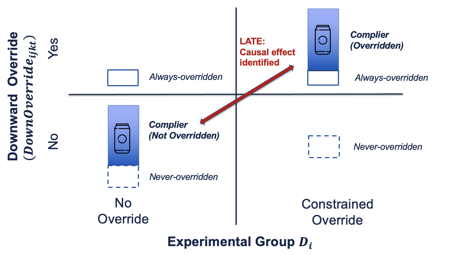
Figure 2 illustrates how LATE is identified through observed override behavior and randomized policy assignment. Each instance falls into one of four quadrants, defined by its override status \(\text{DownOverride}_{ijkt} = \text{DownOverride}_{ijkt}(1) \cdot D_i + \text{DownOverride}_{ijkt}(0) \cdot (1 - D_i)\) and the policy assignment \(D_i \in \{0, 1\}\). Instances that are overridden in the no override group (top-left quadrant) typically reflect extreme scenarios, such as warehouse stockouts. These must be always-overridden cases: given that override is generally prohibited under this policy, any SKU that is still overridden would necessarily be overridden under the constrained condition as well. Overridden cases in the constrained group (top-right quadrant) include a mixture of always-overridden and complier instances. By randomization, the no override group also contains compliers, SKUs that are not overridden but would be if the policy allowed it (bottom-left quadrant). This variation enables identification of the LATE, which captures the causal effect of override decisions for the subset of SKUs whose status is altered by the policy. These are precisely the override decisions that the firm can influence. In this sense, LATE isolates the effect of enabling override discretion for SKUs that would otherwise follow algorithmic suggestions.
Before proceeding to estimation, we clarify how our setting satisfies the core assumptions of the LATE framework. First, the assumption of monotonicity requires that no SKU becomes less likely to be overridden under the constrained override policy than under the no override policy, i.e., \(\text{DownOverride}_{ijkt}(1) \geq \text{DownOverride}_{ijkt}(0)\) for all \(i,j,k,t\). This condition holds by design: the constrained policy either expands override discretion or leaves it unchanged relative to the control, and cannot reduce the probability of an override. Second, the relevance assumption requires that the instrumental variable, randomized policy assignment, affects the likelihood of override. This is satisfied by construction and supported empirically in 4.1, where we show that overrides increase under the constrained condition. Third, the exclusion restriction requires that the policy assignment affects outcomes only through its effect on override behavior. This is justified by the experimental design in 3.3, where all other aspects of the replenishment process are held constant across groups. The only manipulation is the degree of discretionary power over downward override. Accordingly, it is reasonable to assume that any effect of policy assignment on SKU performance operates exclusively through changes in override behavior.
Our formal LATE estimation builds on the main analysis by applying a DID framework within a two-stage least squares (2SLS) specification, using panel data to control for time-invariant heterogeneity. We construct data at the most granular level for each replenish instance \((i, j, k, t)\). To focus on the impact of downward override in particular, we restrict the sample to include only instances where the worker followed or reduced the algorithmic suggestion. We estimate the following two-stage least squares (2SLS) model:
First stage (override decision): \[\textit{DownOverride}_{ijkt} = \pi_0 + \pi_1 (\textit{ConstrainedOverride}_i \cdot \textit{Post}_t) + \gamma_{ij} + \gamma_k + \delta_{c(j)t} + \varepsilon_{ijkt},\] Second stage (outcome consequence): \[Y_{ijkt} = \alpha_0 + \beta_C \cdot \widehat{\textit{DownOverride}}_{ijkt} + \gamma_{ij} + \gamma_k + \delta_{c(j)t} + \varepsilon_{ijkt}.\] In both stages, we include fixed effects at a granular level: \(\gamma_{ij}\) captures worker-machine heterogeneity, \(\gamma_k\) controls for SKU-specific effects, and \(\delta_{c(j)t}\) absorbs city-by-date shocks. Standard errors \(\varepsilon_{ijkt}\) are again clustered at the worker level. Outcome variables are defined consistently with the main analysis but measured at the SKU-replenishment instance and averaged over the period until the next replenishment. We use level outcomes rather than log-transformed outcomes to preserve interpretability of effect magnitudes under the LATE framework. The instrument \(\textit{ConstrainedOverride}_i \cdot \textit{Post}_t\) captures exogenous variation in override behavior induced by policy, and the coefficient \(\beta_C\) identifies the causal effect of downward override for compliers.
| Sales | Sales Probability | Inventory | |
| (Unit: Item) | (\(\%\)) | (Unit: Item) | |
| Constrained vs No Override | |||
| First Stage (Outcome: DownOverride) | |||
| \(ConstrainedOverride_i \cdot Post_{t}\) | \(0.0287^{***} \quad (0.0068)\) | ||
| (Worker-Machine), SKU, (City-Date) FE | Yes | ||
| R\(^2\) | \(0.3272\) | ||
| F-stat | \(5740.2^{***}\) | ||
| Observations | \(7,012,190\) | ||
| Second Stage (LATE) | |||
| \(\widehat{DownOverride}_{ijkt}\) | \(0.2830\) | \(-0.0442\) | \(-3.4456^{***}\) |
| (\(0.3114\)) | (\(0.0937\)) | (\(0.9118\)) | |
| (Worker-Machine), SKU, (City-Date) FE | Yes | Yes | Yes |
| R\(^2\) | \(0.2881\) | \(0.3621\) | \(0.3198\) |
| Observations | \(7,012,190\) | \(7,012,190\) | \(7,012,190\) |
| Free vs No Override | |||
| First Stage (Outcome: DownOverride) | |||
| \(FreeOverride_i \cdot Post_{t}\) | \(0.1292^{***} \quad (0.0140)\) | ||
| (Worker-Machine), SKU, (City-Date) FE | Yes | ||
| R\(^2\) | \(0.3516\) | ||
| F-stat | \(65,405.3^{***}\) | ||
| Observations | \(5,189,189\) | ||
| Second Stage (LATE) | |||
| \(\widehat{DownOverride}_{ijkt}\) | \(-0.1188\) | \(-0.1055^{***}\) | \(-1.2575^{***}\) |
| (\(0.0798\)) | (\(0.0257\)) | (\(0.3055\)) | |
| (Worker-Machine), SKU, (City-Date) FE | Yes | Yes | Yes |
| R\(^2\) | \(0.2806\) | \(0.3545\) | \(0.3183\) |
| Observations | \(5,189,189\) | \(5,189,189\) | \(5,189,189\) |
| Robust standard errors clustered at the worker level. | |||
| \(^{*}p<0.1\); \(^{**}p<0.05\); \(^{***}p<0.01\) | |||
Table 4 estimates the LATE of downward overrides under both the constrained and free override policies, respectively. Relative to the no override group, which exhibits minimal downward overrides, the constrained policy increases override probability by \(2.87\) percentage points (\(F = 5740.2\)), confirming the relevance of the instrument. The second stage shows that these additional overrides reduce inventory by \(3.45\) items on average (\(p < 0.01\)) without significantly affecting either sales quantity or sales probability. In contrast, the free override policy increases override probability by \(12.92\) percentage points (\(F = 65{,}405.3\)), but these overrides lead to less inventory reduction (\(1.26\) items, \(p < 0.01\)) and a significant \(10.6\) percentage point drop in the probability of sale (\(p < 0.01\)).
These contrasting LATE estimates illustrate the central logic of the selective filtering mechanism proposed in 1. Under the free override policy, override decisions reflect a mix of high- and low-quality overrides, leading to a diluted average effect. In contrast, the constrained policy imposes a cardinality limit that forces workers to sort override opportunities and act only on the most promising ones. This endogenous selection process filters out noise and low-quality overrides. As a result, overrides under constraint disproportionately target SKUs with meaningful private signals, improving outcomes at the instance level. These SKU-level gains, in turn, drive the aggregate policy effects predicted by [prop:filtering] and confirmed in Table 1.
Robustness checks in the online appendix 10 further validate the selective filtering mechanism. First, we estimate intent-to-treat (ITT) effects by regressing outcomes directly on policy assignment. Although smaller in magnitude, these effects are directionally consistent with the LATE estimates and reflect average policy impacts across all SKUs, including those not overridden. Second, we tighten the definition of a downward override in the first stage to capture only overrides that reduce SKU inventory to exactly zero. This stricter definition yields substantially larger LATE effects, suggesting that performance gains are concentrated in strongly selective decisions where workers fully remove a SKU from stock. Third, recall that 3 showed a modest increase in upward overrides under the randomized policy. We conduct an ITT analysis restricted to upward override instances and find no significant policy effects, helping to rule out alternative explanations based on general override effort or behavioral spillovers.
Finally, following prior literature [72], [73], we test whether the observed LATE effects reflect worker private information rather than selection based solely on observable SKU characteristics, denoted as \(\mathbf{X}_{ijkt}\). We augment the LATE specification by including instance-level covariates such as sale price and discount status (see details in 14 of the online appendix 10). These features may correlate with override behavior. For example, workers might be more likely to remove a discounted or low-priced SKU, which could mechanically improve inventory performance even without relying on private information. If performance gains were driven solely by such observable features, the inclusion of such covariates would attenuate the estimated LATE effects. Instead, we find that the performance improvements under constrained override persist even after controlling for observables, while the negative effects of free override remain. This result suggests that workers contribute private information beyond what is captured by the algorithm, reinforcing the value of selective filtering.
6 From Mechanism to Practice: Designing Override Policies↩︎
Having established the selective filtering mechanism through theoretical analysis and empirical evidence, we now turn to practical design considerations. Specifically, we examine when override policies are most effective (policy-level heterogeneity) and how override limits might be tailored using data (instance-level learning). These extensions aim to bridge the gap between identifying the mechanism and enabling practical deployment.
| Panel A | Senior Worker | Junior Worker | ||||
| \(\log(\textit{Sales}+1)\) | Sales Probability | \(\log(\textit{Inventory}+1)\) | \(\log(\textit{Sales}+1)\) | Sales Probability | \(\log(\textit{Inventory}+1)\) | |
| (Unit: Item) | (\(\%\)) | (Unit: Item) | (Unit: Item) | (\(\%\)) | (Unit: Item) | |
| \(ConstrainedOverride_i \cdot\) | \(0.0030\) | \(-0.0013\) | \(-0.0172^{***}\) | \(-0.0010\) | \(-0.0014\) | \(-0.0095\) |
| \(Post_{t}\) | \((0.0048)\) | \((0.0033)\) | \((0.0063)\) | \((0.0056)\) | \((0.0044)\) | \((0.0073)\) |
| \(FreeOverride_i \cdot\) | \(-0.0139^{***}\) | \(-0.0163^{***}\) | \(-0.0285^{***}\) | \(-0.0100\) | \(-0.0114^{**}\) | \(-0.0036\) |
| \(Post_{t}\) | \((0.0052)\) | \((0.0042)\) | \((0.0073)\) | \((0.0063)\) | \((0.0047)\) | \((0.0110)\) |
| Worker fixed effects | Yes | Yes | Yes | Yes | Yes | Yes |
| (City-Date) fixed effect | Yes | Yes | Yes | Yes | Yes | Yes |
| R\(^{2}\) | \(0.3409\) | \(0.4661\) | \(0.5080\) | \(0.3142\) | \(0.4531\) | \(0.5177\) |
| Observations | \(386,870\) | \(386,870\) | \(386,870\) | \(264,956\) | \(264,956\) | \(264,956\) |
| Panel B | Top-Sales SKU | Low-Sales SKU | ||||
| \(\log(\textit{Sales}+1)\) | Sales Probability | \(\log(\textit{Inventory}+1)\) | \(\log(\textit{Sales}+1)\) | Sales Probability | \(\log(\textit{Inventory}+1)\) | |
| (Unit: Item) | (\(\%\)) | (Unit: Item) | (Unit: Item) | (\(\%\)) | (Unit: Item) | |
| \(ConstrainedOverride_i \cdot\) | \(0.0017\) | \(-0.0029\) | \(-0.0190^{***}\) | \(-0.0056^{**}\) | \(-0.0044\) | \(-0.0014\) |
| \(Post_{t}\) | \((0.0036)\) | \((0.0019)\) | \((0.0056)\) | \((0.0028)\) | \((0.0031)\) | \((0.0047)\) |
| \(FreeOverride_i \cdot\) | \(-0.0158^{***}\) | \(-0.0161^{***}\) | \(-0.0340^{***}\) | \(-0.0066^{**}\) | \(-0.0126^{***}\) | \(0.0116^{*}\) |
| \(Post_{t}\) | \((0.0041)\) | \((0.0025)\) | \((0.0077)\) | \((0.0033)\) | \((0.0037)\) | \((0.0060)\) |
| Worker fixed effects | Yes | Yes | Yes | Yes | Yes | Yes |
| (City-Date) fixed effect | Yes | Yes | Yes | Yes | Yes | Yes |
| R\(^{2}\) | \(0.1219\) | \(0.0948\) | \(0.1474\) | \(0.3410\) | \(0.4260\) | \(0.4113\) |
| Observations | \(576,123\) | \(576,123\) | \(576,123\) | \(624,627\) | \(624,627\) | \(624,627\) |
| Panel C | Growth-Stage SKU | Mature-Stage SKU | ||||
| \(\log(\textit{Sales}+1)\) | Sales Probability | \(\log(\textit{Inventory}+1)\) | \(\log(\textit{Sales}+1)\) | Sales Probability | \(\log(\textit{Inventory}+1)\) | |
| (Unit: Item) | (\(\%\)) | (Unit: Item) | (Unit: Item) | (\(\%\)) | (Unit: Item) | |
| \(ConstrainedOverride_i \cdot\) | \(0.0021\) | \(-0.0031\) | \(-0.0115^{**}\) | \(-0.0020\) | \(-0.0076^{*}\) | \(-0.0205^{*}\) |
| \(Post_{t}\) | \((0.0040)\) | \((0.0029)\) | \((0.0054)\) | \((0.0084)\) | \((0.0040)\) | \((0.0116)\) |
| \(FreeOverride_i \cdot\) | \(-0.0062\) | \(-0.0145^{***}\) | \(-0.0218^{***}\) | \(-0.0269^{***}\) | \(-0.0252^{***}\) | \(-0.0434^{***}\) |
| \(Post_{t}\) | \((0.0054)\) | \((0.0039)\) | \((0.0076)\) | \((0.0087)\) | \((0.0053)\) | \((0.0140)\) |
| Worker fixed effects | Yes | Yes | Yes | Yes | Yes | Yes |
| Date fixed effect | Yes | Yes | Yes | Yes | Yes | Yes |
| R\(^{2}\) | \(0.2820\) | \(0.4088\) | \(0.4584\) | \(0.1668\) | \(0.1106\) | \(0.1737\) |
| Observations | \(621,497\) | \(621,497\) | \(621,497\) | \(110,507\) | \(110,507\) | \(110,507\) |
| Note. Robust standard errors clustered by each worker are in parentheses. | ||||||
| \(^{*}p<0.1\); \(^{**}p<0.05\); \(^{***}p<0.01\) | ||||||
We examine three sources of heterogeneity that may shape the effectiveness of override policies: worker experience, incentive alignment, and data uncertainty. Panel A of Table 5 shows that senior workers, those with more than one year of tenure, drive both the positive effects of constrained override and the negative effects of free override. Under the constrained override policy, senior workers reduce inventory by \(1.72\%\) (\(p < 0.01\)); under free override, they reduce inventory by \(2.85\%\) but cause a substantial \(1.39\%\) decrease in sales (\(p < 0.01\)). In contrast, junior workers have no significant effects under either policy. Panel B shows that constrained override improves inventory only for top-sales SKUs (\(-1.9\%\), \(p < 0.01\)), while free override harms sales across all SKUs and increases inventory for low-sales SKUs (\(+1.16\%\), \(p < 0.1\)). Panel C examines the SKU lifecycle stage as a proxy for algorithmic uncertainty. Constrained overrides significantly reduce inventory for growth-stage SKUs (\(-1.15\%\), \(p < 0.05\)), with a similar though noisier effect for mature SKUs (\(-2.05\%\), \(p < 0.1\)). Free override, by contrast, leads to sharp performance declines in both groups.
Taken together, these results offer valuable practical insights. Constrained override is most effective when workers have experience, when SKUs are strongly tied to sales incentives, and when algorithmic forecasts are less reliable. These conditions highlight contexts where private information is more likely to be valuable and where filtering it through policy constraints yields the greatest benefit. At the same time, the consistent harm caused by free override, regardless of experience, incentive alignment, or data quality, underscores the risk of granting full discretion.
These findings also contribute to the broader literature on private information in operational settings [41], [74], [75]. Prior studies typically adopt a two-stage approach: first identifying contexts in which private information exists and then integrating it into algorithmic decision-making [20]. Our work complements this stream by using a randomized override policy to simultaneously reveal and assess the value of private information through observed behavior. The heterogeneity results confirm earlier findings that private information is stronger among senior workers [23] and for growth-stage SKUs [6]. Importantly, our results show that the constrained override policy not only identifies contexts with valuable private information but also regulates its application, reducing low-quality overrides even among less experienced workers and in settings where algorithmic forecasts are relatively accurate. This highlights a broader design implication: override policies can function not only as decision levers, but also as filters that shape effective human-AI collaboration under uncertainty.
The heterogeneous treatment effects suggest that the value of override discretion varies across workers and SKUs. However, our current policy imposes a uniform cardinality constraint, which may under-utilize high-quality private information and over-permit noisy overrides. To address this limitation, we develop a data-driven refinement that estimates the likelihood that a given override reflects high-quality judgment. The core idea is to learn SKU selection patterns from the constrained override group, where performance is improved, as a proxy for private information.
First, we seek to train a logistic regression model to distinguish instances that are actually overridden by the constrained group from those intended to be overridden without constraints; the latter, however, are unobservable. Instead, we use the override instances selected by the free override group as a proxy, because the constrained override and free override groups are statistically identical due to randomization in the experimental design. Differences in override behavior reflect the presence or absence of the cardinality constraint. The model utilizes a comprehensive set of features that capture local conditions, worker characteristics, and SKU-level attributes. Each override in the free group is then scored by this model to estimate its probability of resembling an override made under constrained conditions, which reflects the quality of overrides.
Second, we simulate a personalized override policy by accepting only those overrides in the free override group with predicted probabilities above a calibrated threshold. This approach relaxes the fixed limit, allowing workers with stronger override signals to override more SKUs. We design a hypothetical scenario in which local workers make override decisions under the refined solution. Compared to the original constrained policy, the personalized override group achieves a \(9.1\) percentage point increase in sales probability (\(p < 0.01\)) and exhibits greater flexibility in override volume, validating the efficacy of this targeted refinement. We provide full details and implementation in Appendix 11.
7 Conclusion↩︎
We propose a simple, scalable solution to improving human supervision of autonomous AI: a constrained override policy. By imposing a cardinality constraint on discretionary overrides, the policy activates a selective filtering mechanism that preserves high-value private information while filtering out human bias. Unlike approaches that require identifying bias or private information in advance, our method is straightforward to implement and generalizes across settings. In a large-scale field experiment on Fengyi Technology’s smart-vending network, constrained overrides improved inventory efficiency without reducing sales, in contrast to the performance losses observed under the free override policy. Following the experiment, Fengyi Technology scaled the policy to more than \(170,000\) machines and \(5,000\) SKUs across over \(70\) metropolitan areas, contributing to an estimated \(\$1,000,000\) annual reduction in inventory costs.
The effectiveness of constrained override rests on three premises. First, worker incentives should be broadly aligned with the algorithm’s objective; otherwise, override choices may diverge from improving machine performance. Second, workers must possess some private, task-relevant information. Without such information, constrained override can only mitigate the losses of free override and cannot outperform the algorithm decision. Third, the operational context should involve low- to medium-stakes decisions in which algorithms hold primary authority and humans serve as supervisors. In high-stakes domains, strict adherence constraints are impractical, and design efforts should instead focus on improving algorithmic recommendations.
8 Additional Information and Results from Section 3↩︎
8.1 Empirical Context and Experiment Design↩︎


Figure 3: No caption.
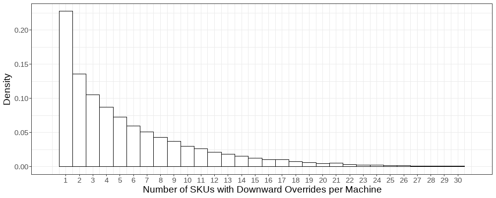
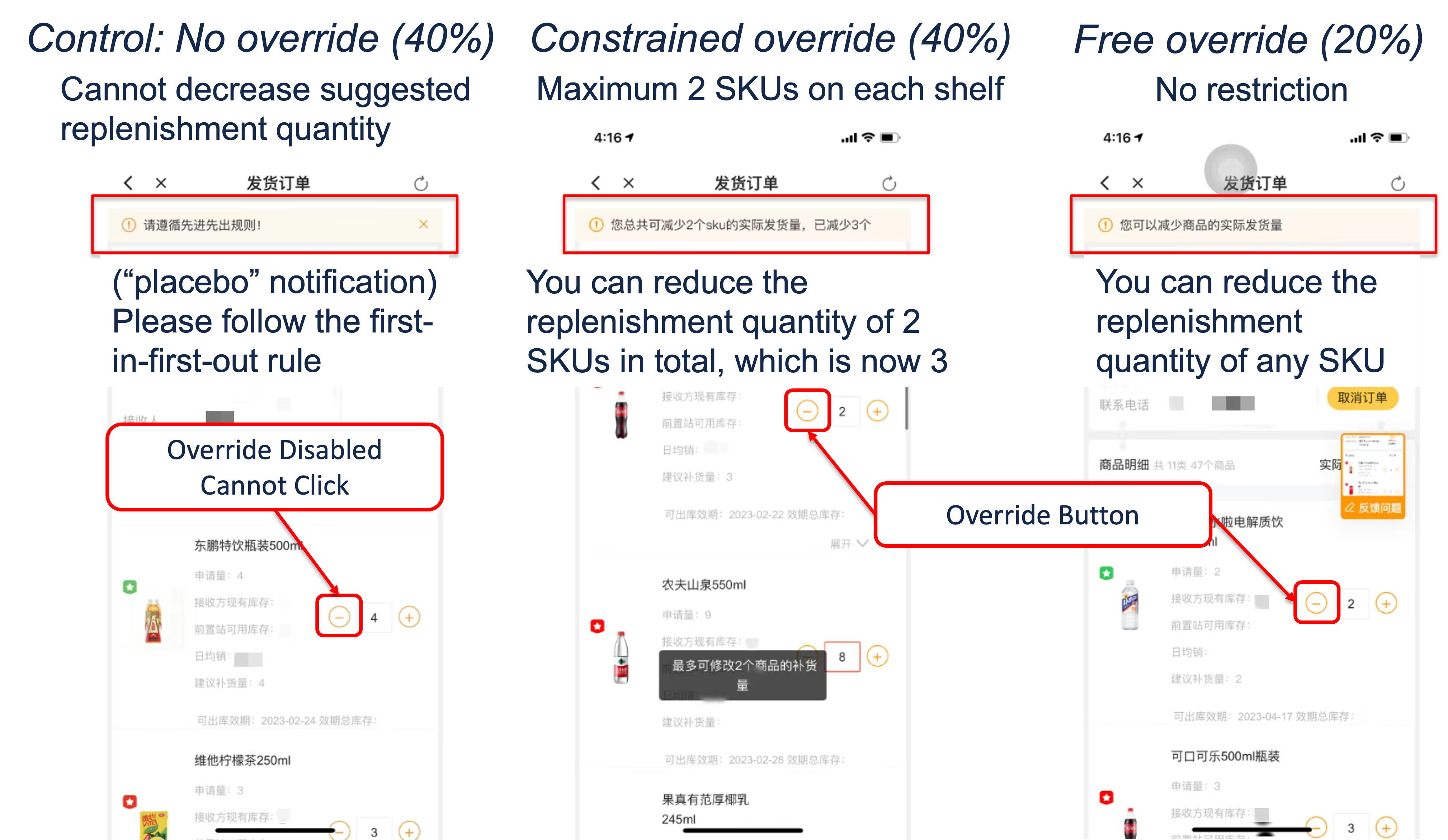
| Means | Differences | |||||
| Feature | No | Constrained | Free | Constrained | Free | Constrained |
| Override | Override | Override | ||||
| Override | Override | Override | \(-\) No | \(-\) No | \(-\) Free | |
| Override | Override | Override | ||||
| Tenure | \(0.710\) | \(0.664\) | \(0.651\) | \(-0.047\) | \(-0.059\) | \(0.012\) |
| (Binary: Senior/Junior) | \([0.455]\) | \([0.474]\) | \([0.479]\) | \((0.044)\) | \((0.055)\) | \((0.056)\) |
| Managed Machines | \(96.757\) | \(94.916\) | \(94.978\) | \(-1.841\) | \(-1.779\) | \(-0.062\) |
| (Unit: Machine) | \([28.222]\) | \([23.971]\) | \([23.922]\) | \((2.486)\) | \((2.976)\) | \((2.798)\) |
| Top-Sales Machines | \(0.137\) | \(0.145\) | \(0.142\) | \(0.008\) | \(0.005\) | \(0.003\) |
| (\(\%\)) | \([0.083]\) | \([0.082]\) | \([0.081]\) | \((0.008)\) | \((0.010)\) | \((0.009)\) |
| Top-Sales SKUs | \(0.174\) | \(0.178\) | \(0.178\) | \(0.004\) | \(0.005\) | \(-0.0003\) |
| (\(\%\)) | \([0.061]\) | \([0.059]\) | \([0.064]\) | \((0.006)\) | \((0.007)\) | \((0.007)\) |
| Growth-Stage SKUs | \(0.554\) | \(0.551\) | \(0.564\) | \(-0.003\) | \(0.010\) | \(-0.013\) |
| (\(\%\)) | \([0.085]\) | \([0.080]\) | \([0.076]\) | \((0.008)\) | \((0.009)\) | \((0.009)\) |
| Average Sales per Machine | \(0.0068\) | \(0.0045\) | \(0.0023\) | |||
| (Unit: Item) | \((0.0080)\) | \((0.0097)\) | \((0.0104)\) | |||
| Average Sales Probability per Machine | Data anonymized | \(0.0023\) | \(0.0016\) | \(0.0007\) | ||
| (\(\%\)) | \((0.0030)\) | \((0.0037)\) | \((0.0037)\) | |||
| Average Inventory per Machine | \(-0.0230\) | \(0.0056\) | \(-0.0286\) | |||
| (Unit: Item) | \((0.0435)\) | \((0.0541)\) | \((0.0557)\) | |||
| Intervened Machines | \(2.796\) | \(3.108\) | \(3.066\) | \(0.312\) | \(0.270\) | \(0.042\) |
| (Unit: Machine) | \([2.952]\) | \([3.038]\) | \([2.963]\) | \((0.284)\) | \((0.346)\) | \((0.349)\) |
| # of Downward SKUs per Machine | \(1.502\) | \(1.710\) | \(1.850\) | \(0.208\) | \(0.348\) | \(-0.140\) |
| (Unit: SKU) | \([1.735]\) | \([2.097]\) | \([2.021]\) | \((0.183)\) | \((0.226)\) | \((0.239)\) |
| \(n\) | \(221\) | \(223\) | \(109\) | |||
| Note. Standard deviations of each group are in brackets, and standard errors are in parentheses. | ||||||
| # of downward SKUs per machine excludes shelf with no (0) downward overrides. | ||||||
| \(^{*}p<0.1\); \(^{**}p<0.05\); \(^{***}p<0.01\) | ||||||
8.2 Proofs of Bayesian Learning Model↩︎
Recall the true prior \(\eta_k \sim \mathcal{N}(\mu, \sigma_\eta^2)\) and the observed signal structure \(s_k = \eta_k + \epsilon_k\) with \(\epsilon_k \sim \mathcal{N}(0,\sigma^2)\). By the conjugate property of normal distributions, the posterior expectation of \(\eta_k\) conditional on the observed signal \(s_k\) is given by: \[\mathbb{E}[\eta_k \mid s_k = s] = \mu + \frac{\sigma_\eta^2}{\tau^2}(s - \mu), \quad \text{where} \quad \tau^2 = \sigma_\eta^2 + \sigma^2.\] Since the posterior expectation is linear in \(s_k\), we apply the law of total expectation to obtain: \[\label{eq:32posterior32expectation} \mathbb{E} \left[\eta_k \mid k \in A^{\text{Constrained}} \right] = \mu + \frac{\sigma_\eta^2}{\tau^2} \left( \mathbb{E} \left[s_k \mid k \in A^{\text{Constrained}} \right] - \mu \right).\tag{2}\]
To compute \(\mathbb{E} \left[s_k \mid k \in A^{\text{Constrained}} \right] = \mathbb{E} [s_k \mid s_k \ge s_{(K)} ]\), we can reparameterize each signal as \(s_k = \mu + \tau U_k\), where \(U_k \sim \mathcal{N}(0, 1)\). This transformation maps the selection event onto the top-\(K\) values of the standard normal variables \(U_k\), where each observation’s rank is uniformly distributed. In particular, we have: \[\label{eq:32order32stats} \mathbb{E} [s_k \mid s_k \ge s_{(K)} ] = \mu + \tau \cdot a(K), \quad \text{where} \quad a(K) = \frac{1}{K} \sum_{j = 1}^K \mathbb{E}[U_{(j)}].\tag{3}\]
Substituting 3 into 2 , we obtain: \[\mathbb{E} \left[\eta_k \mid k \in A^{\text{Constrained}} \right] = \mu + \frac{\sigma_\eta^2}{\tau^2} \left( \mathbb{E} [s_k \mid s_k \ge s_{(K)} ] - \mu \right) = \mu + \frac{\sigma_\eta^2}{\tau} \cdot a(K).\] This is strictly positive if \(a(K) > -\mu \cdot \tau / \sigma_\eta^2\), which completes the proof.
We compare the average causal effects of three override policies. Under the no override policy, the worker accepts all algorithm recommendations without overrides. Thus, \(A^{\text{No}} = \emptyset\) and \(\mathbb{E}\left[\sum_{k \in A^{\text{No}}} \eta_k \right] = 0\).
Under the free override policy, the worker overrides SKU \(k\) if \(s_k > 0\). Similar to 1, for any SKU \(k\), we have: \[\mathbb{E} \left[\eta_k \mid k \in A^{\text{Free}} \right] = \mathbb{E}[\eta_k \mid s_k > 0] = \mu + \frac{\sigma_\eta^2}{\tau^2} \left( \mathbb{E}[s_k \mid s_k > 0] - \mu \right).\] Using the standard normal reparameterization \(s_k = \mu + \tau U_k\), with \(U_k \sim \mathcal{N}(0, 1)\), we get: \[\mathbb{E}[s_k \mid s_k > 0] = \mu + \tau \cdot \mathbb{E}[U_k \mid s_k > 0] = \mu + \tau \cdot \mathbb{E}\left[U_k \mid U_k > -\frac{\mu}{\tau}\right] = \mu + \tau \cdot h\left(-\frac{\mu}{\tau}\right),\] where \(h(x) = \frac{\phi(x)}{1-\Phi(x)}\) denotes the inverse Mills ratio for the standard normal distribution. Furthermore, the override probability of SKU \(k\) is \(\mathbb{P}(s_k > 0) = \mathbb{P}(U_k > -\mu / \tau) = \Phi(\mu / \tau)\). Aggregating across all SKUs, the expected total override value under free override is: \[\mathbb{E}\left[\sum_{k \in A^{\text{Free}}} \eta_k \right] = \sum_{k=1}^N \mathbb{P}(s_k > 0) \mathbb{E}[\eta_k \mid s_k > 0] = N \cdot \Phi\left( \frac{\mu}{\tau} \right) \cdot \left( \mu + \frac{\sigma_\eta^2}{\tau} h\left( -\frac{\mu}{\tau} \right) \right).\] This quantity is negative if \(\mu + \frac{\sigma_\eta^2}{\tau} h(-\mu/\tau) < 0\), which simplifies to \(h(-\mu/\tau) < -\mu \tau / \sigma_\eta^2\).
Under the constrained override policy, the worker selects \(K\) SKUs with the highest signals \(s_k\). Applying 1, the expected total override value under constrained override is \[\begin{align} \mathbb{E}\left[\sum_{k \in A^{\text{Constrained}}} \eta_k \right] &= \sum_{k=1}^N \mathbb{P}( s_k \ge s_{(K)} ) \mathbb{E}[\eta_k \mid s_k \ge s_{(K)} ] = K \cdot \left( \mu + \frac{\sigma_\eta^2}{\tau} a(K) \right), \end{align}\] which is positive if \(a(K) > -\mu \tau / \sigma_\eta^2\).
Putting all the results together, the desired ordering \(\mathbb{E}[\sum_{k \in A^{\text{Constrained}}} \eta_k] > 0 > \mathbb{E}[\sum_{k \in A^{\text{Free}}} \eta_k]\) holds if \(h\left( - \mu / \tau \right) < -\mu \tau / \sigma_\eta^2 < a(K),\) as stated in the proposition.
Proposition [prop:filtering] characterizes conditions under which the constrained override policy yields strictly positive expected override value, whereas the free override policy results in negative expected value on average. To build intuition, we explore these conditions under limiting regimes. For the free override policy, the total expected override value is negative if \(h(-\mu/\tau) + \mu \tau / \sigma_\eta^2 < 0\). In the limiting case where \(\mu \to 0\), this expression approaches \(\sqrt{2/\pi}\), rendering the condition invalid. This outcome aligns with a scenario of unbiased worker beliefs, where the human bias vanishes, and free overrides thus enhance overall performance. Under the constrained override policy, the total expected override value is strictly positive if \(a(K) + \mu \tau / \sigma_\eta^2 > 0\). In the extreme (\(\mu\to-\infty\) or \(\sigma \to +\infty\)), the condition inevitably fails, consistent with scenarios in which the worker’s prior is excessively negatively biased or their observations are entirely noisy. Under these conditions, the worker possesses no valuable private information, and any override would degrade performance.
By Lemma 1, consider the expected total private information extracted under the constrained override policy as a function of the override cap \(K\): \[V(K) = K \cdot \left( \mu + \frac{\sigma_\eta^2}{\tau} a(K) \right),\] where \(a(K) = \frac{1}{K} \sum_{j = 1}^{K} \mathbb{E}[U_{(j)}]\), and \(U_k = (s_k - \mu)/\tau \sim \mathcal{N}(0,1)\). Under the free override policy, the expected number of overrides is: \[\mathbb{E}[K_{\text{free}}] = N \cdot \mathbb{P}(s_k > 0) = N \cdot \Phi\left( \frac{\mu}{\tau} \right).\] Define \(\bar{K} = \lceil \mathbb{E}[K_{\text{free}}] \rceil\) as the smallest integer greater than or equal to this expectation. Our goal is to show \(V(K) \leq 0\) for \(K \geq \bar{K}\), implying the optimal cap \(K^*\) must lie below \(\bar{K}\).
First, observe that for any \(K \ge \bar{K}\): \[a(K) \le a(\bar{K}) \le \mathbb{E} \left[U \Bigl| U > \Phi^{-1} \left( 1 - \frac{\bar{K}}{N} \right) \right] = h \left( \Phi^{-1} \left(1 - \frac{\bar{K}}{N} \right) \right).\] The first inequality follows from the fact that \(a(\cdot)\) is non-increasing in \(K\). The second inequality leverages standard properties of order statistics from a standard normal distribution (see [76], Equation (4)). Next: \[h\left( \Phi^{-1} \left(1 - \frac{\bar{K}}{N}\right) \right) \le h\left( \Phi^{-1} \left(1 - \Phi\left( \frac{\mu}{\tau} \right) \right) \right) = h\left( -\frac{\mu}{\tau} \right),\] since \(h(\cdot)\) and \(\Phi^{-1}(\cdot)\) are both strictly increasing [77], and by definition \(\bar{K} \ge \mathbb{E}[K_{\text{free}}] = N\cdot\Phi(\mu / \tau)\). Therefore, for \(K \geq \bar{K}\), we have: \[\mu + \frac{\sigma_\eta^2}{\tau} a(K) \leq \mu + \frac{\sigma_\eta^2}{\tau} h\left( -\frac{\mu}{\tau} \right) < 0,\] which immediately implies \(V(K) \le 0\). Thus, the optimal cap \(K^*\) must be strictly less than \(\bar{K}\).
8.3 A Rational Inattention Model↩︎
We develop a Rational Inattention (RI) model as an alternative microfoundation for override behavior. Whereas the main model assumes that workers receive private signals of fixed precision and make override decisions subject to an exogenous cardinality constraint, the RI framework [31], [32] endogenizes both signal quality and attention allocation. By doing so, it provides a behavioral foundation for a selective override mechanism grounded in cognitive frictions. Crucially, we show that even when signal formation is endogenous, imposing a structural cap on override actions can still improve decision quality through a sorting effect analogous to that in the main model.
To ensure comparability, we retain the same task environment. The worker replenishes a set of \(N\) SKUs indexed by \(k \in \{1, \dots, N\}\). The individual causal effect of overriding SKU \(k\) is \(\eta_k \sim \mathcal{N}(\mu, \sigma^2)\). Consistent with empirical patterns in override performance, we assume \(\mu < 0\), implying that override decisions are systematically biased downward on average. Departing from the baseline Bayesian setup, we now assume that the worker endogenously chooses a uniform attention level \(\lambda \in \Lambda \subseteq [0, +\infty)\), which determines the precision of the signal observed for each SKU. The observed signal is \(s_k = \eta_k + \epsilon_k\), where \(\epsilon_k \sim \mathcal{N}(0, 1/\lambda)\) captures processing noise, and signal variance is \(\sigma^2 + 1/\lambda\). Greater attention improves signal quality but increases cognitive cost. Following standard RI models [32], we assume that the cost of attention is proportional to mutual information. Since all SKUs share the same attention level, the total cost is \(\kappa N \cdot \frac{1}{2} \log(1 + \lambda \sigma^2)\), where \(\kappa > 0\) denotes the marginal cost of information. After observing the signal vector \(\{s_k\}\), the worker chooses a subset \(A \subseteq \{1, \dots, N\}\) of SKUs to override. Consistent with earlier assumptions, we assume the worker ignores the negative prior bias and sets \(\mu = 0\) in forming beliefs. The worker’s objective is to maximize expected override value net of cognitive cost: \[\max_{\lambda \in \Lambda, A} \quad \mathbb{E}\left[\sum_{k \in A} \eta_k \right] - \kappa N \cdot \tfrac{1}{2} \log(1 + \lambda \sigma^2).\]
Given a fixed attention level \(\lambda\), he worker’s optimal override choices under each policy remain identical to those derived in Section 3.2. Specifically, let \(A^{\text{Constrained}}(\lambda)\), \(A^{\text{Free}}(\lambda)\), and \(A^{\text{No}}(\lambda)\) denote optimal override sets under constrained, free, and no-override regimes respectively. We summarize the policies as follows:
No override policy: the worker must follow all algorithmic recommendations \(A^{\text{No}}(\lambda) = \emptyset\) and chooses \(\lambda = 0\), resulting in no override actions and no attention cost.
Free override policy: the worker first sets an attention level \(\lambda \in \Lambda\). Based on the observation of the signal \(s_k = \eta_k + \epsilon_k\), the worker overrides each SKU with a positive observed signal: \(A^{\text{Free}}(\lambda) = \{k : s_k > 0\}\). Attention level \(\lambda\) is chosen to maximize expected net override value.
Constrained override policy: after setting the attention level \(\lambda \in \Lambda\), the worker chooses at most \(K\) overrides by selecting SKUs with the largest positive signals: \(A^{\text{Constrained}}(\lambda) = \{k : s_k \ge s_{(K)}, s_k > 0\}\). Similarly, we consider the approximation \(A^{\text{Constrained}}(\lambda) \approx \{k : s_k \ge s_{(K)}\}\). Then, \(\lambda\) is optimized to maximize expected net override value.
By restricting actions to SKUs with the strongest signals, the constrained policy implements selective filtering, improving override quality. We now formalize the resulting ranking across policies.
Let \(\lambda^{\text{Constrained}}\), \(\lambda^{\text{Free}}\), and \(\lambda^{\text{No}}\) denote the optimal attention levels under the constrained, free, and no-override policies, respectively. Then the expected total override values satisfy: \[\mathbb{E}\left[\sum_{k \in A^{\text{Constrained}}(\lambda^{\text{Constrained}})} \eta_k \right] > \mathbb{E}\left[\sum_{k \in A^{\text{No}}(\lambda^{\text{No}})} \eta_k \right] = 0 > \mathbb{E}\left[\sum_{k \in A^{\text{Free}}(\lambda^{\text{Free}})} \eta_k \right]\] if \(h(-\mu/\sqrt{\sigma^2 + 1/\lambda}) < -\mu \sqrt{\sigma^2 + 1/\lambda} / \sigma_\eta^2 < a(K)\) for any \(\lambda \in \Lambda\).
By [prop:filtering], for any fixed attention level \(\lambda \in \Lambda\), if \(a(K) > -\mu \sqrt{\sigma^2 + 1/\lambda} / \sigma_\eta^2\), then: \[\mathbb{E}\left[\sum_{k \in A^{\text{Constrained}}(\lambda)} \eta_k \right] > 0.\] Selecting the optimal attention level \(\lambda^{\text{Constrained}}\), which maximizes the worker’s objective under the constrained override regime, immediately yields the stated result. A parallel argument applies directly to the free override regime, establishing the negative expected value under optimal attention \(\lambda^{\text{Free}}\).
9 Additional Analyses for Section 4↩︎
Figure 6 plots the daily average machine-level sales (top panel) and inventory levels (bottom panel). Each point represents the average value across all treated machines operated by active workers in that group on a given day. The data span April \(1\) to June \(18\), \(2023\), with the vertical line indicating May \(4\), \(2023\), the start of the experimental override policies. Prior to treatment, the three groups exhibit parallel trends, consistent with the random assignment of override policies at the worker level. After the intervention, meaningful differences emerge. The constrained override group achieves the highest average sales while maintaining moderate inventory levels. The free override group holds the lowest inventory but suffers from lower sales, suggesting excessive reductions.
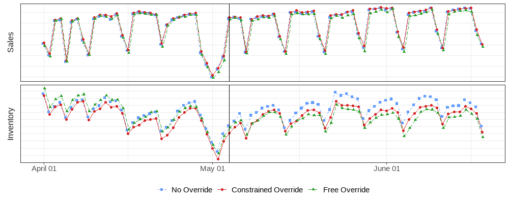
9.1 Main Policy Effect↩︎
This section reports several robustness checks to support our main findings in 4. Table 7 presents results obtained by re-estimating our models using level outcomes rather than log-transformed variables. The results remain consistent with our main findings. Constrained override causes a statistically significant reduction in inventory (\(-0.0860\), \(p < 0.05\)) and a small, positive, but statistically insignificant effect on sales. In contrast, free override leads to both a significant inventory reduction (\(-0.1452\), \(p < 0.01\)) and a significant decline in sales (\(-0.0327\), \(p < 0.05\)). These patterns reinforce the conclusion that while both override policies reduce inventory, only the constrained override avoids the negative sales impact observed under free override.
| Sales | Inventory | |
| (Unit: Item) | (Unit: Item) | |
| \(Constrained\;Override_i \times Post\;Treatment_{t}\) | \(0.0084\) | \(-0.0860^{**}\) |
| \(\) | \((0.0169)\) | \((0.0408)\) |
| \(Free\;Override_i \times Post\;Treatment_{t}\) | \(-0.0327^{**}\) | \(-0.1452^{***}\) |
| \(\) | \((0.0162)\) | \((0.0524)\) |
| Worker fixed effects | Yes | Yes |
| (City-Date) fixed effect | Yes | Yes |
| R\(^{2}\) | \(0.1739\) | \(0.1039\) |
| Observations | \(639,112\) | \(639,112\) |
| Note. Robust standard errors clustered by each worker are in parentheses. | ||
| \(^{*}p<0.1\); \(^{**}p<0.05\); \(^{***}p<0.01\) | ||
Table 8 verifies robustness to temporal variation by excluding weekends and public holidays. The results again support our main claims. Specifically, constrained override has no significant effect on sales (measured either as log quantity or as binary sales probability), but it continues to reduce inventory significantly (\(-0.0117\), \(p < 0.05\)). Free override, by contrast, results in a statistically significant decline across all three metrics, log sales (\(-0.0128\), \(p < 0.01\)), sales probability (\(-0.0145\), \(p < 0.01\)), and inventory (\(-0.0220\), \(p < 0.01\)). The consistent negative effects of free override on sales across specifications further underscore its unintended consequence of reduced performance, while highlighting the effectiveness of constrained override in improving efficiency without negatively impacting sales.
| \(\log(\textit{Sales}+1)\) | Sales Probability | \(\log(\textit{Inventory}+1)\) | |
| (Unit: Item) | (\(\%\)) | (Unit: Item) | |
| \(Constrained\;Override_i \times Post\;Treatment_{t}\) | \(0.0018\) | \(-0.0022\) | \(-0.0117^{**}\) |
| \(\) | \((0.0039)\) | \((0.0028)\) | \((0.0050)\) |
| \(Free\;Override_i \times Post\;Treatment_{t}\) | \(-0.0128^{***}\) | \(-0.0145^{***}\) | \(-0.0220^{***}\) |
| \(\) | \((0.0042)\) | \((0.0033)\) | \((0.0065)\) |
| Worker fixed effects | Yes | Yes | Yes |
| (City-Date) fixed effect | Yes | Yes | Yes |
| R\(^{2}\) | \(0.1651\) | \(0.1881\) | \(0.1681\) |
| Observations | \(532,592\) | \(532,592\) | \(532,592\) |
| Note. Robust standard errors clustered by each worker are in parentheses. | |||
| \(^{*}p<0.1\); \(^{**}p<0.05\); \(^{***}p<0.01\) | |||
| \(\log(\textit{Sales}+1)\) | Sales Probability | \(\log(\textit{Inventory}+1)\) | |
| (Unit: Item) | (\(\%\)) | (Unit: Item) | |
| \(Constrained\;Override_i \times Pre \;Week\;1_t\) | \(0.0008\) | \(-0.0022\) | \(-0.0037\) |
| \((0.0048)\) | \((0.0029)\) | \((0.0059)\) | |
| \(Constrained\;Override_i \times Post\;Week\;0_t\) | \(0.0028\) | \(-0.0001\) | \(-0.0155^{***}\) |
| \((0.0031)\) | \((0.0029)\) | \((0.0054)\) | |
| \(Constrained\;Override_i \times Post\;Week\;1_t\) | \(0.0016\) | \(-0.0007\) | \(-0.0045\) |
| \((0.0038)\) | \((0.0029)\) | \((0.0061)\) | |
| \(Constrained\;Override_i \times Post\;Week\;2_t\) | \(-0.0027\) | \(-0.0036\) | \(-0.0147^{**}\) |
| \((0.0041)\) | \((0.0032)\) | \((0.0064)\) | |
| \(Constrained\;Override_i \times Post\;Week\;3_t\) | \(-0.0006\) | \(-0.0030\) | \(-0.0160^{**}\) |
| \((0.0047)\) | \((0.0034)\) | \((0.0065)\) | |
| \(Constrained\;Override_i \times Post\;Week\;4_t\) | \(-0.0003\) | \(-0.0067^{*}\) | \(-0.0130^{*}\) |
| \((0.0062)\) | \((0.0038)\) | \((0.0068)\) | |
| \(Constrained\;Override_i \times Post\;Week\;5_t\) | \(0.0013\) | \(-0.0032\) | \(-0.0162^{**}\) |
| \((0.0063)\) | \((0.0050)\) | \((0.0076)\) | |
| \(Constrained\;Override_i \times Post\;Week\;6_t\) | \(0.0099\) | \(0.0050\) | \(-0.0128\) |
| \((0.0097)\) | \((0.0076)\) | \((0.0092)\) | |
| \(Free\;Override_i \times Pre \;Week\;1_t\) | \(-0.0010\) | \(-0.0036\) | \(-0.0060\) |
| \((0.0049)\) | \((0.0029)\) | \((0.0064)\) | |
| \(Free\;Override_i \times Post\;Week\;0_t\) | \(-0.0055\) | \(-0.0063^{*}\) | \(-0.0154^{**}\) |
| \((0.0039)\) | \((0.0034)\) | \((0.0060)\) | |
| \(Free\;Override_i \times Post\;Week\;1_t\) | \(-0.0039\) | \(-0.0088^{***}\) | \(-0.0152^{**}\) |
| \((0.0044)\) | \((0.0033)\) | \((0.0075)\) | |
| \(Free\;Override_i \times Post\;Week\;2_t\) | \(-0.0115^{**}\) | \(-0.0166^{***}\) | \(-0.0109\) |
| \((0.0051)\) | \((0.0039)\) | \((0.0084)\) | |
| \(Free\;Override_i \times Post\;Week\;3_t\) | \(-0.0153^{***}\) | \(-0.0177^{***}\) | \(-0.0136^{*}\) |
| \((0.0050)\) | \((0.0040)\) | \((0.0081)\) | |
| \(Free\;Override_i \times Post\;Week\;4_t\) | \(-0.0171^{***}\) | \(-0.0194^{***}\) | \(-0.0260^{***}\) |
| \((0.0060)\) | \((0.0047)\) | \((0.0085)\) | |
| \(Free\;Override_i \times Post\;Week\;5_t\) | \(-0.0189^{***}\) | \(-0.0199^{***}\) | \(-0.0343^{***}\) |
| \((0.0072)\) | \((0.0060)\) | \((0.0102)\) | |
| \(Free\;Override_i \times Post\;Week\;6_t\) | \(-0.0114\) | \(-0.0077\) | \(-0.0333^{***}\) |
| \((0.0104)\) | \((0.0089)\) | \((0.0108)\) | |
| Worker fixed effects | Yes | Yes | Yes |
| (City-Date) fixed effect | Yes | Yes | Yes |
| R\(^{2}\) | \(0.1751\) | \(0.2073\) | \(0.1708\) |
| Observations | \(639{,}112\) | \(639{,}112\) | \(639{,}112\) |
| Note. Robust standard errors clustered by each worker are in parentheses. | |||
| \(^{*}p<0.1\); \(^{**}p<0.05\); \(^{***}p<0.01\) | |||
9 reports the results of the following weekly DID model: \[\label{eq:did95machine95dynamic} \begin{align} \textit{Outcome}_{ijt} = \alpha &+ \beta_{1,-1} (\textit{ConstrainedOverride}_i \cdot \textit{PreWeek1}_t) + \sum_{w=0}^{6} \delta_{1w} (\textit{ConstrainedOverride}_i \cdot \textit{PostWeek}_{wt}) \\ &+ \beta_{2,-1} (\textit{FreeOverride}_i \cdot \textit{PreWeek1}_t) + \sum_{w=0}^{6} \delta_{2w} (\textit{FreeOverride}_i \cdot \textit{PostWeek}_{wt}) \\ &+ \gamma_i + \delta_{c(j)t} + \varepsilon_{ijt}. \end{align}\tag{4}\] Specifically, we interact each treatment group indicator with week-specific dummies for the seven weeks following the intervention, along with a pre-treatment lag term to assess potential pre-trends. We find no evidence of significant pre-treatment differences, further validating the randomization procedure. After the intervention, the free override group exhibits an immediate and sustained decline in both sales and sales probability, while the constrained group achieves a meaningful reduction in inventory without reducing sales. The persistence of these effects suggests that override behavior reflects systematic overrides in decision-making rather than transitory noise.
Corresponding to the analyses in 4.1, Table 10 reports weekly DID estimates for algorithm suggestions. The constrained override group shows no significant change throughout. The free override group exhibits a marked increase in suggested quantity per machine beginning after Week 0. These findings suggest that the algorithm adapts to aggressive quantity reductions under free override by increasing future replenishment recommendations, without broadening the product mix. This supports our interpretation that the algorithm response is not a general reaction to override policy, but rather a targeted response to systematic over-reduction.
| Quantity per Machine | SKU per Machine | Quantity per SKU | |
| (Unit: Item) | (\(\%\)) | (Unit: Item) | |
| \(Constrained\;Override_i \times Post\;Week\;0_t\) | \(0.0199\) | \(0.0257\) | \(0.0213\) |
| \((1.0510)\) | \((0.1979)\) | \((0.0393)\) | |
| \(Constrained\;Override_i \times Post\;Week\;1_t\) | \(1.1871\) | \(-0.0052\) | \(0.0599\) |
| \((1.0766)\) | \((0.2096)\) | \((0.0441)\) | |
| \(Constrained\;Override_i \times Post\;Week\;2_t\) | \(0.7990\) | \(-0.0360\) | \(0.0525\) |
| \((1.0643)\) | \((0.1966)\) | \((0.0408)\) | |
| \(Constrained\;Override_i \times Post\;Week\;3_t\) | \(1.9995^{*}\) | \(0.1982\) | \(0.0703\) |
| \((1.1639)\) | \((0.2159)\) | \((0.0470)\) | |
| \(Constrained\;Override_i \times Post\;Week\;4_t\) | \(0.7336\) | \(-0.0392\) | \(0.0571\) |
| \((1.3331)\) | \((0.2330)\) | \((0.0499)\) | |
| \(Constrained\;Override_i \times Post\;Week\;5_t\) | \(0.0005\) | \(-0.1597\) | \(0.0473\) |
| \((1.3461)\) | \((0.2449)\) | \((0.0513)\) | |
| \(Constrained\;Override_i \times Post\;Week\;6_t\) | \(0.7487\) | \(-0.1849\) | \(0.1433^{**}\) |
| \((1.5158)\) | \((0.2770)\) | \((0.0619)\) | |
| \(Free\;Override_i \times Post\;Week\;0_t\) | \(0.7786\) | \(0.0452\) | \(0.1196^{*}\) |
| \((1.5799)\) | \((0.2828)\) | \((0.0617)\) | |
| \(Free\;Override_i \times Post\;Week\;1_t\) | \(4.3356^{**}\) | \(0.4092\) | \(0.2525^{***}\) |
| \((1.7832)\) | \((0.3208)\) | \((0.0729)\) | |
| \(Free\;Override_i \times Post\;Week\;2_t\) | \(3.6646^{**}\) | \(0.1849\) | \(0.2223^{***}\) |
| \((1.8503)\) | \((0.3166)\) | \((0.0738)\) | |
| \(Free\;Override_i \times Post\;Week\;3_t\) | \(3.3012^{*}\) | \(0.1934\) | \(0.1822^{**}\) |
| \((1.7478)\) | \((0.3116)\) | \((0.0746)\) | |
| \(Free\;Override_i \times Post\;Week\;4_t\) | \(3.5809^{*}\) | \(0.1388\) | \(0.2437^{***}\) |
| \((2.0951)\) | \((0.3521)\) | \((0.0818)\) | |
| \(Free\;Override_i \times Post\;Week\;5_t\) | \(3.8801^{*}\) | \(0.2758\) | \(0.2543^{***}\) |
| \((2.0326)\) | \((0.3683)\) | \((0.0829)\) | |
| \(Free\;Override_i \times Post\;Week\;6_t\) | \(4.4855^{**}\) | \(0.3279\) | \(0.3053^{***}\) |
| \((2.2517)\) | \((0.3931)\) | \((0.0919)\) | |
| Worker fixed effects | Yes | Yes | Yes |
| (City-Date) fixed effect | Yes | Yes | Yes |
| R\(^{2}\) | \(0.1938\) | \(0.2100\) | \(0.2105\) |
| Observations | \(639{,}112\) | \(639{,}112\) | \(639{,}112\) |
| Note. Robust standard errors clustered by each worker are in parentheses. | |||
| \(^{*}p<0.1\); \(^{**}p<0.05\); \(^{***}p<0.01\) | |||
9.2 Changes in Override Behavior↩︎
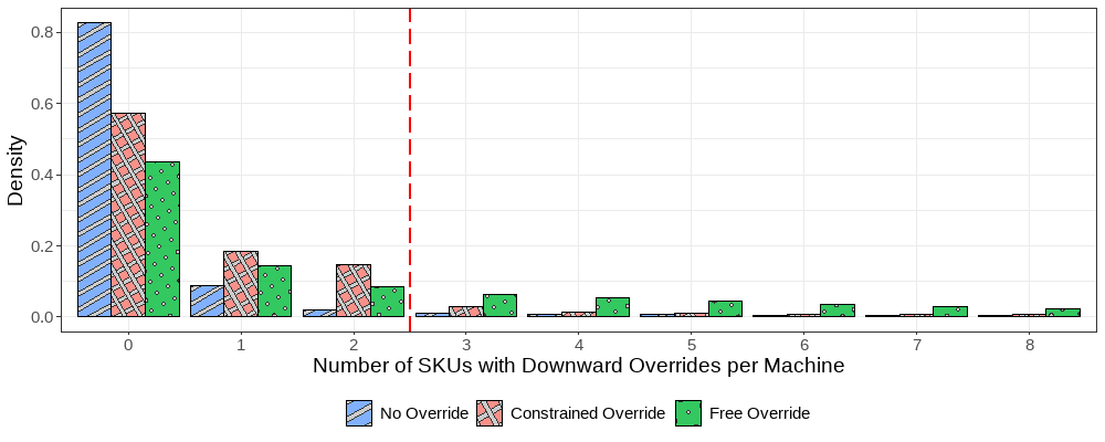
7 shows the distribution of downward overrides per machine-day across policy groups. As expected, the no override group exhibits near-zero override activity, with rare exceptions likely due to stockouts or edge cases. The free override group frequently overrides multiple SKUs, while the constrained group shows a sharp concentration at one to two overrides, consistent with the policy cap of \(K=2\). Again, although the cap is not strictly enforced, instances of exceedance are rare and symmetrically distributed across groups due to worker-level randomization.
10 Additional Analyses from Section 5↩︎
This section provides several robustness checks to support the main LATE findings. First, Table 11 reports intent-to-treat (ITT) estimates using policy assignment as the regressor. The ITT results follow the same pattern as the LATE estimates: the constrained policy reduces inventory (\(-0.099\), \(p<0.01\)) without affecting sales, while the free policy reduces inventory (\(-0.163\), \(p<0.01\)) but simultaneously lowers the probability of sale (\(-0.0136\), \(p<0.01\)). As expected, the ITT effects are smaller in magnitude, but they reinforce the conclusion that constrained overrides improve performance through selective filtering, while free overrides degrade it.
| Sales | Sales01 | Inventory | |
| (Unit: Item) | (\(\%\)) | (Unit: Item) | |
| Constrained vs No Override | |||
| \(Constrained\;Override_i \cdot Post_{t}\) | \(0.0081\) | \(-0.0013\) | \(-0.0990^{***}\) |
| (\(0.0089\)) | (\(0.0027\)) | (\(0.0262\)) | |
| (Worker-Machine), SKU, (City-Date) FE | Yes | Yes | Yes |
| R\(^2\) | \(0.2881\) | \(0.3621\) | \(0.3198\) |
| Observations | \(7,012,190\) | \(7,012,190\) | \(7,012,190\) |
| Free vs No Override | |||
| \(Free\;Override_i \cdot Post_{t}\) | \(-0.0154\) | \(-0.0136^{***}\) | \(-0.1625^{***}\) |
| (\(0.0103\)) | (\(0.0033\)) | (\(0.0395\)) | |
| (Worker-Machine), SKU, (City-Date) FE | Yes | Yes | Yes |
| R\(^2\) | \(0.2806\) | \(0.3545\) | \(0.3183\) |
| Observations | \(5,189,189\) | \(5,189,189\) | \(5,189,189\) |
| Robust standard errors clustered at the worker level. | |||
| \(^{*}p<0.1\); \(^{**}p<0.05\); \(^{***}p<0.01\) | |||
Second, we redefine the treatment to focus on a stricter class of override decisions, those that reduce inventory to exactly zero, while keeping the full sample unchanged. As shown in Table 12, the estimated effects are substantially larger in magnitude, as expected. Under the constrained policy, zero-out overrides reduce inventory by an average of \(8.85\) items (\(p<0.01\)), compared to \(3.45\) items in the main specification, with no significant sales loss. Under the free policy, inventory falls by \(5.22\) items (\(p<0.01\)) and sales probability drops by \(43.8\) percentage points (\(p<0.01\)). The magnitude of the inventory reduction is substantially larger under this stricter definition, \(8.85\) items versus \(3.45\) in the baseline, confirming that zero-out overrides represent more decisive and high-impact interventions. Likewise, the negative sales effect under free override intensifies from \(10.6\) to \(43.8\) percentage points, highlighting the risks associated with unconstrained discretion in overaggressive overrides.
| Sales | Sales01 | Inventory | |
| (Unit: Item) | (\(\%\)) | (Unit: Item) | |
| Constrained vs No Override | |||
| First Stage (Outcome: DownOverride0) | |||
| \(ConstrainedOverride_i \cdot Post_{t}\) | \(0.0112^{***} \quad (0.0029)\) | ||
| (Worker-Machine), SKU, (City-Date) FE | Yes | ||
| R\(^2\) | \(0.3210\) | ||
| F-stat | \(2738.5^{***}\) | ||
| Observations | \(7,012,190\) | ||
| Second Stage (LATE) | |||
| \(\widehat{DownOverride0}_{ijkt}\) | \(0.7261\) | \(-0.1136\) | \(-8.8548^{***}\) |
| (\(0.8002\)) | (\(0.2407\)) | (\(2.3431\)) | |
| (Worker-Machine), SKU, (City-Date) FE | Yes | Yes | Yes |
| R\(^2\) | \(0.2881\) | \(0.3621\) | \(0.3198\) |
| Observations | \(7,012,190\) | \(7,012,190\) | \(7,012,190\) |
| Free vs No Override | |||
| First Stage (Outcome: DownOverride0) | |||
| \(FreeOverride_i \cdot Post_{t}\) | \(0.0312^{***} \quad (0.0049)\) | ||
| (Worker-Machine), SKU, (City-Date) FE | Yes | ||
| R\(^2\) | \(0.2691\) | ||
| F-stat | \(12,538.5^{***}\) | ||
| Observations | \(5,189,189\) | ||
| Second Stage (LATE) | |||
| \(\widehat{DownOverride0}_{ijkt}\) | \(-0.4929\) | \(-0.4377^{***}\) | \(-5.2162^{***}\) |
| (\(0.3309\)) | (\(0.1067\)) | (\(1.2675\)) | |
| (Worker-Machine), SKU, (City-Date) FE | Yes | Yes | Yes |
| R\(^2\) | \(0.2806\) | \(0.3545\) | \(0.3183\) |
| Observations | \(5,189,189\) | \(5,189,189\) | \(5,189,189\) |
| Robust standard errors clustered at the worker level. | |||
| \(^{*}p<0.1\); \(^{**}p<0.05\); \(^{***}p<0.01\) | |||
Third, Table 13 reports ITT estimates on a restricted sample consisting only of upward override instances. This specification tests whether override policies influence performance outcomes for SKUs whose replenishment quantities were increased rather than decreased. All coefficients are small and statistically insignificant across sales, sales probability, and inventory, indicating no meaningful effect of policy assignment on SKU performance in the upward direction. This null result helps rule out alternative explanations based on general override effort or broader behavioral changes, reinforcing that the main effects are specific to downward override behavior and consistent with selective filtering rather than general override activity.
| Sales | Sales01 | Inventory | |
| (Unit: Item) | (\(\%\)) | (Unit: Item) | |
| Constrained vs No Override | |||
| \(ConstrainedOverride_i \cdot Post_{t}\) | \(0.0380\) | \(0.0002\) | \(-0.0640\) |
| (\(0.0277\)) | (\(0.0036\)) | (\(0.0549\)) | |
| (Worker-Machine), SKU, (City-Date) FE | Yes | Yes | Yes |
| R\(^2\) | \(0.3235\) | \(0.1980\) | \(0.3787\) |
| Observations | \(1,639,664\) | \(1,639,664\) | \(1,639,664\) |
| Free vs No Override | |||
| \(FreeOverride_i \cdot Post_{t}\) | \(-0.0290\) | \(-0.0002\) | \(-0.0294\) |
| (\(0.0217\)) | (\(0.0044\)) | (\(0.0716\)) | |
| (Worker-Machine), SKU, (City-Date) FE | Yes | Yes | Yes |
| R\(^2\) | \(0.3077\) | \(0.1994\) | \(0.3648\) |
| Observations | \(1,187,107\) | \(1,187,107\) | \(1,187,107\) |
| Robust standard errors clustered at the worker level. | |||
| \(^{*}p<0.1\); \(^{**}p<0.05\); \(^{***}p<0.01\) | |||
Finally, 14 augments the LATE specification by including instance-level covariates. As we can see, the estimated inventory reduction under constrained override remains large and significant (\(-3.50\) items, \(p < 0.01\)), nearly identical to the baseline estimate (\(-3.45\) in Table 4), indicating that workers act on information beyond algorithm-accessible features. In contrast, for the free override policy, inventory reductions become only modestly weaker (\(-1.48\) vs. \(-1.26\)), but the negative sales effect remains large and significant (\(-11.0\) percentage points, \(p < 0.01\)), suggesting that unconstrained override decisions continue to degrade performance even after conditioning on observed SKU characteristics.
| Sales | Sales Probability | Inventory | |
| (Unit: Item) | (\(\%\)) | (Unit: Item) | |
| Constrained vs No Override | |||
| First Stage (Outcome: DownOverride) | |||
| \(ConstrainedOverride_i \cdot Post_{t}\) | \(0.0287^{***}\) (\(0.0068\)) | ||
| Discounted | \(-0.0070^{***}\) (\(0.0011\)) | ||
| Sale Price | \(0.0035^{***}\) (\(0.0009\)) | ||
| Danger Flag | \(-0.0069^{***}\) (\(0.0010\)) | ||
| Growth SKU | \(-0.0080^{***}\) (\(0.0012\)) | ||
| Top SKU \(\cdot\) Top Shelf | \(-0.0188^{***}\) (\(0.0020\)) | ||
| Top SKU | \(0.0357^{***}\) (\(0.0032\)) | ||
| Top Shelf | \(0.0097^{***}\) (\(0.0021\)) | ||
| Tenure | \(0.1158\) (\(0.3584\)) | ||
| (Worker-Machine), SKU, (City-Date) FE | Yes | ||
| R\(^2\) | \(0.3297\) | ||
| F-stat | \(3,575.6^{***}\) | ||
| Observations | \(7,012,190\) | ||
| Second Stage (LATE) | |||
| \(\widehat{DownOverride}_{ijkt}\) | \(0.2703\) (\(0.3109\)) | \(-0.0469\) (\(0.0949\)) | \(-3.4958^{***}\) (\(0.8496\)) |
| Discounted | \(-0.0009\) (\(0.0054\)) | \(0.0093^{***}\) (\(0.0011\)) | \(0.8500^{***}\) (\(0.0291\)) |
| Sale Price | \(-0.1199^{***}\) (\(0.0066\)) | \(-0.0098^{***}\) (\(0.0005\)) | \(-0.4889^{***}\) (\(0.0183\)) |
| Danger Flag | \(-0.0024\) (\(0.0044\)) | \(0.0084^{***}\) (\(0.0010\)) | \(0.7205^{***}\) (\(0.0218\)) |
| Growth SKU | \(-0.0960^{***}\) (\(0.0056\)) | \(-0.0101^{***}\) (\(0.0015\)) | \(-0.6266^{***}\) (\(0.0208\)) |
| Top SKU \(\cdot\) Top Shelf | \(0.1885^{***}\) (\(0.0107\)) | \(-0.0569^{***}\) (\(0.0022\)) | \(-0.8131^{***}\) (\(0.0345\)) |
| Top SKU | \(0.3055^{***}\) (\(0.0124\)) | \(0.0887^{***}\) (\(0.0036\)) | \(3.8991^{***}\) (\(0.0457\)) |
| Top Shelf | \(-0.0947^{***}\) (\(0.0071\)) | \(0.0419^{***}\) (\(0.0022\)) | \(0.2845^{***}\) (\(0.0262\)) |
| Tenure | \(0.5528\) (\(1.0395\)) | \(0.0227\) (\(0.1210\)) | \(0.2060\) (\(1.0550\)) |
| (Worker-Machine), SKU, (City-Date) FE | Yes | Yes | Yes |
| R\(^2\) | \(0.3022\) | \(0.3698\) | \(0.4133\) |
| Observations | \(7,012,190\) | \(7,012,190\) | \(7,012,190\) |
| Free vs No Override | |||
| First Stage (Outcome: DownOverride) | |||
| \(FreeOverride_i \cdot Post_{t}\) | \(0.1292^{***}\) (\(0.0140\)) | ||
| Discounted | \(-0.0076^{***}\) (\(0.0014\)) | ||
| Sale Price | \(0.0036^{***}\) (\(0.0011\)) | ||
| Danger Flag | \(-0.0077^{***}\) (\(0.0012\)) | ||
| Growth SKU | \(-0.0079^{***}\) (\(0.0013\)) | ||
| Top SKU \(\cdot\) Top Shelf | \(-0.0235^{***}\) (\(0.0029\)) | ||
| Top SKU | \(0.0488^{***}\) (\(0.0045\)) | ||
| Top Shelf | \(0.0052^{**}\) (\(0.0026\)) | ||
| Tenure | \(-0.0253\) (\(0.5195\)) | ||
| (Worker-Machine), SKU, (City-Date) FE | Yes | ||
| R\(^2\) | \(0.3555\) | ||
| F-stat | \(10,729.3^{***}\) | ||
| Observations | \(5,189,189\) | ||
| Second Stage (LATE) | |||
| \(\widehat{DownOverride}_{ijkt}\) | \(-0.1423^{*}\) (\(0.0805\)) | \(-0.1101^{***}\) (\(0.0262\)) | \(-1.4750^{***}\) (\(0.3213\)) |
| Discounted | \(-0.0009\) (\(0.0070\)) | \(0.0085^{***}\) (\(0.0011\)) | \(0.9187^{***}\) (\(0.0363\)) |
| Sale Price | \(-0.1102^{***}\) (\(0.0058\)) | \(-0.0098^{***}\) (\(0.0005\)) | \(-0.4933^{***}\) (\(0.0202\)) |
| Danger Flag | \(-0.0080\) (\(0.0049\)) | \(0.0071^{***}\) (\(0.0010\)) | \(0.7508^{***}\) (\(0.0243\)) |
| Growth SKU | \(-0.1081^{***}\) (\(0.0087\)) | \(-0.0117^{***}\) (\(0.0014\)) | \(-0.6403^{***}\) (\(0.0281\)) |
| Top SKU \(\cdot\) Top Shelf | \(0.1757^{***}\) (\(0.0109\)) | \(-0.0607^{***}\) (\(0.0020\)) | \(-0.7497^{***}\) (\(0.0390\)) |
| Top SKU | \(0.3178^{***}\) (\(0.0075\)) | \(0.0919^{***}\) (\(0.0021\)) | \(3.8015^{***}\) (\(0.0423\)) |
| Top Shelf | \(-0.0890^{***}\) (\(0.0084\)) | \(0.0461^{***}\) (\(0.0020\)) | \(0.2397^{***}\) (\(0.0297\)) |
| Tenure | \(-0.0805\) (\(0.6144\)) | \(-0.3038\) (\(0.3209\)) | \(4.3243\) (\(1.7150\)) |
| (Worker-Machine), SKU, (City-Date) FE | Yes | Yes | Yes |
| R\(^2\) | \(0.2943\) | \(0.3621\) | \(0.4102\) |
| Observations | \(5,189,189\) | \(5,189,189\) | \(5,189,189\) |
| Robust standard errors clustered at the worker level. | |||
| \(^{*}p<0.1\); \(^{**}p<0.05\); \(^{***}p<0.01\) | |||
11 Additional Information for Section 6↩︎
To learn how the constrained override group selects SKUs for downward overrides, we develop a logistic regression model at the instance level to estimate the probability that an SKU is selected by the constrained override group from SKUs intended to be overridden without constraints. However, the SKUs that the constrained override group would likely override in the absence of constraints are unobservable. We therefore use the SKUs selected by the free override group as a proxy because the constrained override and free override groups are statistically identical due to randomization in the experimental design. The training data consists of all observed downward overrides from constrained and free override groups, indexed by \((i,j,k,t)\) for worker, machine, SKU, and time, with instances \((x_{ijkt}, y_{ijkt})\). The feature vector \(x_{ijkt}\) captures worker, machine, and SKU characteristics, and the label \(y_{ijkt}\) indicates the group: \(y_{ijkt}=1\) for constrained-group overrides and \(y_{ijkt}=0\) for free-group overrides.
We employ features that could potentially influence the override selection process. First, we include features displayed in the app (Figure 5) when local workers make override decisions, such as the current inventory level, weekly sales, and the suggested replenishment quantity of the SKU. These features are the most direct messages that local workers receive when making override decisions. Additionally, we include the actual replenishment quantity of the SKU to capture the magnitude of override decisions. Second, we incorporate features that describe basic information about local workers, vending machines, and SKUs. We selected features in collaboration with Fengyi Technology based on their business insights regarding factors that may influence override decisions. Examples include the tenure of local workers, the type of environment where smart vending machines are located, top-sales vending machines or SKUs, danger flags for SKUs at risk of removal due to low sales, and whether SKUs are categorized as growth-stage SKUs. All features used in the regression are listed in Table ¿tbl:table:32feature32explanation?, along with detailed explanations. Figure 8 presents the importance scores for the top \(15\) most essential features that correlate with private information, such as the top-sales SKU and location of the smart vending machines.
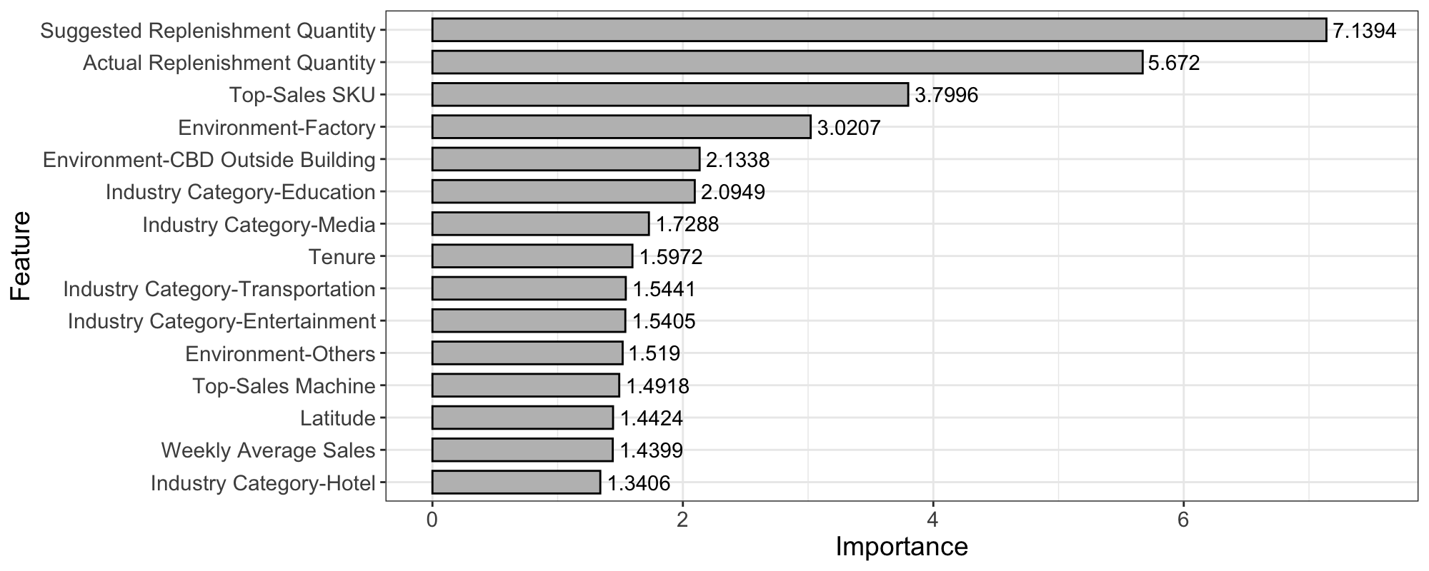
Leveraging the trained logistic regression, we implement an instance-level “Accept or Reject" policy for candidate downward overrides. The key idea is to keep proposed overrides that are more likely to be selected by the constrained override group. We outline a hypothetical scenario in which local workers make override decisions under the refined policy. Before replenishing, local workers receive a list of SKUs with suggested replenishment quantities. They identify a set of SKUs to override and submit for approval by the centralized server. The centralized server then computes \(\hat{p}_{ijkt}\) for each SKU, the estimated probability that would be selected by the constrained override group, and sets a threshold \(\alpha \in (0,1)\): overrides with \(\hat{p}_{ijkt} \ge \alpha\) are accepted, whereas those with \(\hat{p}_{ijkt} < \alpha\) are rejected. This selection process personalizes the cardinality constraints across different workers and times.
We simulate the hypothetical scenario using the randomized experimental data. Because workers in the free override group faced no downward constraint, their observed overrides serve as the pool of proposed overrides to the centralized server. Using the trained logistic regression, we compute \(\hat{p}_{ijkt}\) for each override instance and retain those with \(\hat{p}_{ijkt} \ge 0.63\). We set the threshold \(\alpha=0.63\) so that the mean number of decreased SKUs is approximately equal in the constrained override and personalized override groups, thereby focusing on distributional differences. This procedure generates a new group of data, referred to as the personalized override group (\(n=100\)), which applies customized constraints tailored to each instance. We aim to compare performance between the constrained override group (fixed constraints) and the personalized override group (personalized constraints). Random assignment in the experimental design ensures the groups are statistically identical before override decisions, supporting a fair comparison.
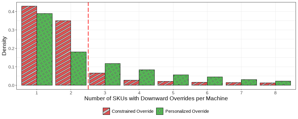
Figure 9 presents the distributions of the average number of decreased SKUs for the two groups. The red dashed line marks the threshold of \(2\) SKUs per machine, representing the fixed constraint imposed on the constrained override group. As expected, the histogram for the constrained override group shows a sharp decline beginning at \(3\) SKUs. In contrast, the histogram for the personalized override group exhibits a heavier tail beyond \(2\) SKUs. The difference confirms the design of the refined solution, where personalized constraints are applied to different instances, allowing local workers with stronger private information to override more than \(2\) SKUs per machine.
Then, we analyze the performance difference between the constrained and personalized override groups, focusing on sales probability at the override instance level. Figure 10 draws the distributions of averaged sales probability among vending machines, SKUs, and time for the two groups. The distribution of the personalized override group shifts to the right compared to the constrained override group. We also conduct a \(t\)-test to estimate the differences in sales probability at the worker level. The personalized override group exhibits an increase in sales probability by \(9.1\) percentage point (\(p\)-value \(<0.01\)). These findings validate the effectiveness of the refined solution, which learns from SKU selection under the constrained override policy, thereby further supporting our explanation in Section 3.2.