1 Introduction↩︎

Competitive equilibrium (CE) is one of the central solution concepts in market design and microeconomic theory. The Fisher market is one of the most fundamental market settings. In a classical Fisher market with goods, there is a set of \(m\) goods and \(n\) agents. Each agent is endowed with a fixed budget of money, and once prices are assigned to the goods, agents spend their budgets to obtain utility-maximizing bundles. Prices are at equilibrium when these individual demands exactly clear the market. Beyond the static existence and welfare properties of CE, a classical question asks whether natural market dynamics can find such prices. Walrasian tâtonnement is the canonical example: prices are adjusted in response to excess demand, increasing when demand exceeds supply and decreasing when supply exceeds demand [2]. The stability and convergence of such dynamics have been studied since the foundational work of [3]–[5], and remain active topics in algorithmic game theory [6]–[10].

This paper studies tâtonnement dynamics in Fisher markets with chores. In a chores market, agents do not pay to receive goods; rather, they are paid to perform undesirable tasks. Thus prices represent payments per unit of work, and the natural response to imbalance is reversed: when a chore is under-demanded, its price should increase to attract agents, while an over-demanded chore should become less lucrative. This reversal leads to a substantially different dynamical landscape. Chores markets can have disconnected sets of equilibria, and excess demand no longer has the monotonic structure that supports many goods-market analyses. Correspondingly, the computational literature on chores and mixed manna deals with non-convex optimization issues and is more nuanced than in the goods case [11]–[16].

Relative Tâtonnement. The recent work of [1] initiated the study of tâtonnement dynamics for chores markets. They show that the naïve additive analogue of tâtonnement can diverge, even in simple chores markets, and propose relative tâtonnement, which restores convergence by subtracting the average excess-demand signal from each coordinate. Relative tâtonnement shows that it is indeed possible to recover convergence for a tâtonnement-like procedure, but at the cost of a global normalization to excess demand. Crucially, this normalization requires each price to be updated with knowledge of the excess-demand signals of all other chores, making relative tâtonnement not fully distributed: it is a centrally coordinated adjustment process rather than a truly decentralized one.

The Appeal of Decoupled Price-Adjustment Dynamics. Economically, the tatonnement process simulates how prices adjust in real markets: each good has a manager, auctioneer, or a market-maker who observes only the imbalance between supply and demand for that good, and adjusts its price accordingly. This decentralized vision is precisely what makes tatonnement a compelling model of market dynamics — it does not require a central planner who aggregates information across all goods, nor does it require any individual agent to know the global state of the market. Each price responds only to its own local signal, and equilibrium emerges as a collective consequence of many independent local adjustments. This is, in Hayek’s terms [17], the informational miracle of the price system: global co-ordination is achieved through purely local price updates.

Our paper asks whether there exist truly decoupled tâtonnement dynamics for the chores setting? We answer this question in the affirmative by giving a multiplicative update in which each chore reacts only to its own excess demand signal. Our dynamics, which we call multiplicative tâtonnement, updates each chore price according to \[p_j^{k+1} = p_j^k(1 + \eta^k y_j^k),\] where \(y_j^k\) is the excess supply of chore \(j\) at the current prices \(p_j^k\)s. The update is fully local: the manager of chore \(j\) only needs to know the current payment \(p_j^k\) and the imbalance signal \(y_j^k\) for that chore. No average excess-demand term, price-simplex projection, or information about other chores is used. The key observation is that the correction imposed explicitly by relative tâtonnement emerges implicitly from the multiplicative update. When prices are initialized in the budget simplex, Walras’ law makes the multiplicative dynamics preserve the relevant aggregate price geometry while still allowing each coordinate to update independently.

1.1 Our Contributions↩︎

We make four main contributions.

1. First, we introduce multiplicative tâtonnement as a fully distributed market dynamics for chores Fisher markets.

2. Second, we prove that this dynamics converges to a CE for general continuous, convex, and \(1\)-homogeneous (CCH) disutilities (Theorem 1). The proof relates the update to entropic mirror descent, while controlling the perturbation created by using the simple multiplicative rule rather than the exact exponential update that is induced by entropic mirror descent.

3. Third, for convex CES disutilities, we prove convergence rates to approximate CE using a relative-smoothness argument on the price simplex (Theorem 2). This yields the same \(O(1/\varepsilon^2)\) dependence on the approximation parameter \(\epsilon\) as relative tâtonnement, with improved dependence on problem constants, while avoiding any coupling.

4. Finally, we compare the dynamics empirically on real-world and simulated instances, and find that multiplicative tâtonnement substantially outperforms relative tâtonnement in practice (Section 5).

1.2 Related work↩︎

Economic dynamics in goods markets. The study of economic dynamics in goods markets has been prevalent in the theoretical computer science community since the 2000s, often with a focus on algorithmic complexity. The first polynomial-time algorithm for linear Fisher markets, introduced by [18], uses a primal-dual approach that can be interpreted as an economic dynamics. In the more general setting of exchange economies satisfying weak gross substitutability (WGS), [6] showed that discrete-time additive tâtonnement dynamics converges to an approximate equilibrium. [7], [19] showed that multiplicative tâtonnement dynamics with artificial upper bounds on excess demand converges in certain nonlinear constant elasticity of substitution (CES) markets. Along this line of research, [8]–[10], [20] further improved convergence rates for a wide range of markets.

Economic dynamics and optimization. Tâtonnement dynamics is often connected to first-order methods through the well-known Eisenberg–Gale convex program [21]–[23]. In [24], the authors show that even classic proximal gradient descent can have an economic-dynamics interpretation. There is also recent work on price-adjustment dynamics related to other optimization methods [25], [26]. Proportional response (PR) dynamics is another popular class of economic dynamics, known to converge to a CE for CES utilities in goods markets [27], [28]. [29] shows that PR dynamics is equivalent to mirror descent on the convex Shmyrev program [30]. Better convergence rates and generalized versions of PR dynamics have also been established [31], [32]. For a detailed survey of proportional response dynamics, we refer the reader to [33]. Recent work [34] also studies market dynamics, including tâtonnement and proportional response dynamics, for public goods.

CE in chores markets. In contrast to goods markets, computing a CE in chores markets is known to be harder [14]. This difficulty stems from the “poles” in the classic Eisenberg-Gale (EG) program for chores markets, and economic dynamics inherits this difficulty [1], [11], [13]. [16] opened up a direction for developing useful optimization algorithms by introducing a dual EG program without the “pole” issue. Later, a general version of this dual EG program was discovered for continuous, convex, \(1\)-homogeneous chores markets [1], [34]. [1] prove a rate of \(\tilde{\mathcal{O}}(1/\varepsilon^2)\) for computing an approximate CE in a wide range of CES chores markets.

2 Preliminaries↩︎

2.0.0.1 Chores Fisher Markets.

A chores Fisher market consists of a set of \(n\) agents and a set of \(m\) divisible chores. Agents are deciding on what chores to take on from in order to earn money. Each agent \(i\) incurs a disutility \(d_i (\mathbf{x}_i)\) for a bundle \(\mathbf{x}_i = (x_{i1}, x_{i2}, \dots, x_{im})\) of chores that is assigned to her, where \(x_{ij}\) represents the amount of chore \(j\) allocated to agent \(i\). Each agent \(i\) has an earning requirement of \(B_i > 0\). We consider each \(d_i: \mathbb{R}^m_+ \rightarrow \mathbb{R}_+\) to be a general continuous, convex, \(1\)-homogeneous (CCH) disutility function, and \(d_i(\mathbf{x}_i) > 0\) for any nonzero \(\mathbf{x}_i\). We call such markets as CCH chores Fisher markets.

Each chore \(j\) has a fixed supply \(s_j > 0\). An allocation is denoted by a matrix \(\mathbf{x}\in \mathbb{R}^{n \times m}_{+}\) whose \(i\)th row is \(\mathbf{x}_i\). Given prices \(\mathbf{p}= (p_1, \dots, p_m)\) of chores, where \(p_j\) represents the payment-per-unit of chore \(j\) done, agent \(i\) will demand a bundle of chores that minimizes her disutility subject to satisfying her earning requirements, i.e., the demand of agent \(i\) is denoted by \[X_i(\mathbf{p}) := \textrm{argmin}_{\mathbf{x}'_i \in \mathbb{R}^m_+} \left\{ d_i(\mathbf{x}'_i) \mid \inp*{\mathbf{p}}{\mathbf{x}'_i} \geq B_i \right.\}.\] A competitive equilibrium of a chores Fisher market is defined as follows.

Without loss of generality, we make the following assumptions.

We show in 7 that any CCH chores Fisher market can be scaled to satisfy the above assumption, and that this scaling induces a bijection between the sets of CE of the two markets. We further make the following natural assumption on disutility functions.

Under 2, no agent would do a zero-priced task, and therefore, it must be that \(p^*_j>0\) for all \(j\in [m]\) at equilibrium to ensure that every chore is done. As a result, the market clearing condition reduces to \(\sum_{i = 1}^n x_{ij} = 1\) for all \(j \in [m]\). In this paper, we consider the following approximate CE [1].

That is, only the market clearing condition is approximately satisfied, the rest of the equilibrium conditions are satisfied exactly. A common class of CCH disutility functions is the class of convex CES disutilities: \[d_i(\mathbf{x}_i) = \Big( \sum\nolimits_{j = 1}^m (d_{ij} x_{ij})^\rho \Big)^{\frac{1}{\rho}}, \quad d_{ij} > 0 \;\forall \;j \in [m], \, \rho \in (1, \infty). \] Convex CES disutilities are CCH, strictly positive for any nonzero \(\mathbf{x}_i\), and satisfy 2.

2.0.0.2 Excess Supply and Tâtonnement Dynamics.

For a given price vector \(\mathbf{p}\in \mathbb{R}^m_+\), the excess supply mapping is defined as (excess-demand is negative of excess-supply) \[Y(\mathbf{p}) = \Big\{ \mathbf{1}_m - \sum\nolimits_{i = 1}^n \mathbf{x}_i \;\Big| \;\mathbf{x}_i \in X_i(\mathbf{p}) \Big\}.\] We call any \(\mathbf{y}\in Y(\mathbf{p})\) an excess supply (vector). If there exists a \(\mathbf{y}\in Y(\mathbf{p})\) such that \(\mathbf{y}= \mathbf{0}_m\), then \(\mathbf{p}\) corresponds to a CE. If there exists a \(\mathbf{y}\in Y(\mathbf{p})\) such that \(\norm{\mathbf{y}}_2 \leq \varepsilon\), then \(\mathbf{p}\) corresponds to an \(\varepsilon\)-approximate CE defined in 2; we add a proof these facts in 7 for completeness.

Tâtonnement dynamics is a price-adjustment process driven by excess supply. Intuitively, in a chores Fisher market, if the supply of a chore exceeds the demand for it, then the price of the chore should be increased to attract more agents to take on the chore. Conversely, if the supply is below the demand, then the price should be decreased so that agents become less willing to perform the chore. [1] considered two types of tâtonnement dynamics: \[\begin{align} \mathbf{y}^k &\in Y(\mathbf{p}^k) \\ \mathbf{p}^{k + 1} &= \mathbf{p}^k + \eta^k \mathbf{y}^k, \end{align}\label{alg:naive-ttm}\tag{1}\] and \[\begin{align} \mathbf{y}^k &\in Y(\mathbf{p}^k) \\ \tilde{\mathbf{y}}^k &= \mathbf{y}^k - \big( \frac{1}{m} \mathbf{1}_m^\top \mathbf{y}^k \big) \cdot \mathbf{1}_m \\ \mathbf{p}^{k + 1} &= \mathbf{p}^k + \eta^k \tilde{\mathbf{y}}^k. \end{align}\label{alg:relative-ttm}\tag{2}\] They show that, 1 dynamics can diverge in chores Fisher markets with convex CES disutilities, whereas 2 dynamics converges in any CCH chores Fisher market satisfying 2.

2.0.0.3 Mirror descent.

Let \(h: \mathbb{R}^m \rightarrow \mathbb{R}\) be a function that is: a) strictly convex, b) continuously differentiable, c) defined on a closed convex set. Then, the Bregman divergence is defined as \[D_h(\mathbf{p}, \mathbf{q}) = h(\mathbf{p}) - h(\mathbf{q}) - \langle \nabla h(\mathbf{q}), \mathbf{p}- \mathbf{q}\rangle.\] If we takes \(h_{\textrm{KL}}(\mathbf{p}) = \sum_{j = 1}^m p_j \log{p_j}\), \(D_{\textrm{KL}}(\mathbf{p}, \mathbf{q}) = \sum_{j = 1}^m p_j \log{\frac{p_j}{q_j}} - p_j + q_j\), which is classic relative entropy, or KL divergence. Mirror descent is a first-order optimization method that uses a Bregman divergence as its proximal geometry. Given a differentiable objective \(f: \mathcal{P} \rightarrow \mathbb{R}\) and \(\mathcal{P} \subset \mathbb{R}^m\), mirror descent updates \[\mathbf{p}^{k + 1} = \textrm{argmin}_{\mathbf{p}\in \mathcal{P}} \left\{ \eta^k \inp{\nabla f(\mathbf{p}^k)}{\mathbf{p}} + D_h(\mathbf{p}, \mathbf{p}^k) \right\}.\] Relative smoothness generalizes the usual Lipschitz-gradient smoothness condition. We say that \(f\) is \(L\)-smooth relative to \(h\) if \[f(\mathbf{q}) \leq f(\mathbf{p}) + \inp{\nabla f(\mathbf{p})}{\mathbf{q}- \mathbf{p}} + L D_h(\mathbf{q}, \mathbf{p}), \quad \textrm{ for all } \mathbf{p}, \mathbf{q}\in \mathcal{P}.\]

3 Multiplicative tâtonnement and its convergence↩︎

3.1 Multiplicative tâtonnement dynamics↩︎

We begin by introducing a new dynamics for chores Fisher market. For each chore \(j\), suppose there is a manager \(j\) responsible for allocating that chore among the agents. In each round \(k\), manager \(j\) submits a payment-per-unit \(p^k_j\) to the market and receive an excess-supply signal \(y^k_j\). She then updates the payment-per-unit multiplicatively in response to this signal: if there is positive excess supply (more of the chore is supplied than agents want to perform), she increases the payment, and vice versa. The update in round \(k\) can be written compactly as follows, where \(\odot\) denotes coordinate-wise product, and \(\eta^k\) is the step size: \[\begin{align} \mathbf{y}^k &\in Y(\mathbf{p}^k) \\ \mathbf{p}^{k + 1} &= \mathbf{p}^k \odot (\mathbf{1}_m + \eta^k \mathbf{y}^k). \end{align}\label{alg:mul-ttm}\tag{3}\]

This multiplicative dynamics has two key advantages:

• It is fully distributed: each manager observes only the feedback associated with her own chore, and not the feedback associated with other chores.

• It scales the adjustment by both the excess-supply signal and the current payment-per-unit.

3.2 Asymptotic convergence of multiplicative tâtonnement↩︎

Next, we prove that, 3 dynamics converges to a CE in any CCH chores Fisher market. This fact is in contrast to its additive analogue as Naïve Tâtonnement is known to provably diverge across a family of CCH chores Fisher markets [1].

One major obstacle to guaranteeing convergence of dynamics to a CE in chores markets is the divergent behavior of prices once they leave the “price simplex”, as pointed out by [1]. In contrast to approaches that impose a correction on the excess-supply signal, multiplicative tâtonnement prevents price divergence by exploiting Walras’ law, a fundamental identity in general equilibrium theory. All proofs in this section are deferred to 8.

By leveraging this intrinsic property of excess supply, the price vectors generated by multiplicative tâtonnement automatically stay within the affine hull of \(\Delta_B\), if the initial price vector lies in \(\Delta_B\). Beyond this fact, to ensure convergence of the dynamics, we additionally require boundedness of the excess supply and strict positivity of the prices.

Define \(\ell_0 = \frac{1}{3m} \min_{i} \big\{ \min \{{d'_{ij}}/{d'_{ij'}}\;|\;{j, j' \in [m]}, \tilde{x}_{ij} \geq \frac{1}{2 n m}, \tilde{x}_{ij'} \leq 2m B_i, \mathbf{d}'_i \in \partial d_i(\tilde{\mathbf{x}}_i) \} \big\} > 0\).

We then prove the convergence of multiplicative tâtonnement by linking it to the following updates: \[\bar{\mathbf{p}}^{k + 1} := \mathbf{p}^k \odot \exp{(\eta \mathbf{y}^k)}, \label{eq:entropy-ttm}\tag{4}\] which is mirror descent w.r.t. the relative entropy for the following objective function [1] \[f(\mathbf{p}) := - \displaystyle\sum_{j = 1}^m p_j + \sum_{i = 1}^n B_i \log\left( \max_{\mathbf{x}_i \geq 0: d_i(\mathbf{x}_i) \leq 1} \inp{\mathbf{p}}{\mathbf{x}_i} \right). \label{def:function-f}\tag{5}\] Note that 4 itself does not converge since the function \(f\) is not globally lower bounded. In particular, the objective value goes to \(-\infty\) as \(\mathbf{p}\rightarrow \mathbf{0}_m\), or as \(p_j \rightarrow \infty\) for any \(j \in [m]\). However, it serves as a useful reference process for proving the per-step improvement: multiplicative tâtonnement tracks 4 within the price simplex \(\Delta_B\), and thus inherits the iterate descent property up to a small perturbation. Since \(f\) is lower bounded within \(\Delta_B\), the iterate converges to a stationary point asymptotically.

Formally, 3 dynamics fits into the following Bregman subgradient update scheme [35]: \[\mathbf{p}^{k + 1} \approx \textrm{argmin}_{\mathbf{q}} \{ \eta^k \inp{-\mathbf{y}^k}{\mathbf{q}} + D_{\textrm{KL}}(\mathbf{q}\Vert \mathbf{p}^k) \}, \label{eq:bregman-subgradient-update-1}\tag{6}\] and the perturbation error is controlled by \[\norm*{\frac{\nabla h_{\textrm{KL}}(\mathbf{p}^{k + 1}) - \nabla h_{\textrm{KL}}(\mathbf{p}^k)}{\eta^k} - \mathbf{y}^k}_2 \leq \nu^k. \label{eq:bregman-subgradient-update-2}\tag{7}\]

[35] prove the convergence of the above process under a set of regularity conditions. We adapt their result to our setting and state it as the following proposition.

Therefore, by combining 1 2, and choosing the proper stepsizes to control the perturbation error, we can prove the convergence of 3 .

4 Convergence rates to an approximate CE under convex CES disutilities↩︎

We further study convergence rates of multiplicative tâtonnement to find an \(\varepsilon\)-approximate CE. We focus on the class of convex CES disutility function, i.e., \(d_i(\mathbf{x}_i) = (\sum_{j = 1}^m (d_{ij} x_{ij})^\rho)^{1/\rho}\) with \(\rho \in (1, \infty)\). Since the inner-log maximization problem in 5 ensures its value bounded away from zero, and has a unique maximizer, function \(f\) is differentiable: \[f(\mathbf{p}) = - \sum_{j = 1}^m p_j + \sum_{i = 1}^n \frac{B_i}{\sigma} \log{\Big( \sum_{j = 1}^m d_{ij}^{-\sigma} p_j^\sigma \Big)}, \quad \sigma = \frac{\rho}{\rho - 1} \in (1, \infty).\]

To study the convergence rate of 2 dynamics, analyze its smoothness with respect to the squared Euclidean norm, which is the standard notion of smoothness. The convergence rate of 3 dynamics, by contrast, is governed by relative smoothness with respect to \(h_{\textrm{KL}}\). By leveraging the fact that \(\mathbf{p}\in \Delta_B\), we obtain an improved relative smoothness than the standard one. In particular, it establishes the smoothness over entire \(\Delta_B\) for the full spectrum of \(\rho \in (1, \infty)\), and the modulus does not depend on a lower bound on the prices. This relative smoothness then lays the foundation for a tighter convergence rate. All proofs in this section is in 9.

With this tool in hand, we next prove a convergence rate to compute an \(\varepsilon\)-approximate CE. We have \[\mathbf{p}^{k + 1} = \textrm{argmin}_{\mathbf{q}\geq 0} \{ \eta^k \inp{-\mathbf{y}^k + \nu^k}{\mathbf{q}} + D_{\textrm{KL}}(\mathbf{q}\Vert \mathbf{p}^k) \}\] where the perturbation \(\nu^k\) is defined as \[\nu^k := -\frac{\log{(1 + \eta^k \mathbf{y}^k)}}{\eta^k} + \mathbf{y}^k.\]

By standard mirror descent analysis and 3, we have the following descent lemma:

Define \(\norm{\mathbf{y}}_{\mathbf{p}} := \sqrt{\sum_{j=1}^m p_j (y_j)^2}\), we can then link the last two terms in 8 to \(\norm{\mathbf{y}^k}_{\mathbf{p}^k}^2\). To do so, we need the stepsizes to be uniformly small to control \(\norm{\eta^k \mathbf{y}^k}_\infty\).

Combining 4 5 yields the convergence rate.

By taking \(\varepsilon = \sqrt{\ell_0 / 2} \varepsilon\) and \(\eta = {1}/{(12(L + B))}\), we directly have the following corollary.

4.0.0.1 Discussions.

First, 2 shows that we can find a price vector for which \(\sum_{j=1}^m p_j (y_j)^2 \leq \varepsilon\) in \(\mathcal{O}(1/\varepsilon^2)\) iterations, without any dependence on \(1/\ell_0\). In other words, for any price coordinate that is not close to zero, an \(\varepsilon\)-small excess supply is guaranteed. We emphasize that as \(\rho \rightarrow \infty\), \(1/\ell_0\) grows exponentially fast and can therefore be problematic. Since \(L + \beta = (\sigma - 1)m^{\sigma - 1} (\min_{i,j} d_{ij})^{-\sigma} + 1 + (\min_{i,j} d_{ij})^{-1}\), and \(\sigma \rightarrow 1\) as \(\rho \rightarrow \infty\), this convergence rate ensures that multiplicative tâtonnement finds a meaningful price vector even as \(\rho \rightarrow \infty\).

Second, as we detail in 9.1, relative tâtonnement has a dependence of \(\mathcal{O}\big( \frac{(\sigma - 1)(\min_{i,j} d_{ij})^{-(\sigma+1)}}{\sqrt{m}\ell_0 \varepsilon^2} \big)\), even under an analysis sharper than the original one in [1]. In contrast, multiplicative tâtonnement improves this rate by a factor of \((\min_{i,j} d_{ij})^{-1}\). As we will see in 5, this factor dominates in most real-world instances and can be very large.

Third, 1 indicates that we can compute an approximate CE using a constant stepsize that is much larger than that allowed by relative tâtonnement. In 5, we show that this larger stepsize can substantially improve the performance of multiplicative tâtonnement.

5 Numerical experiments↩︎

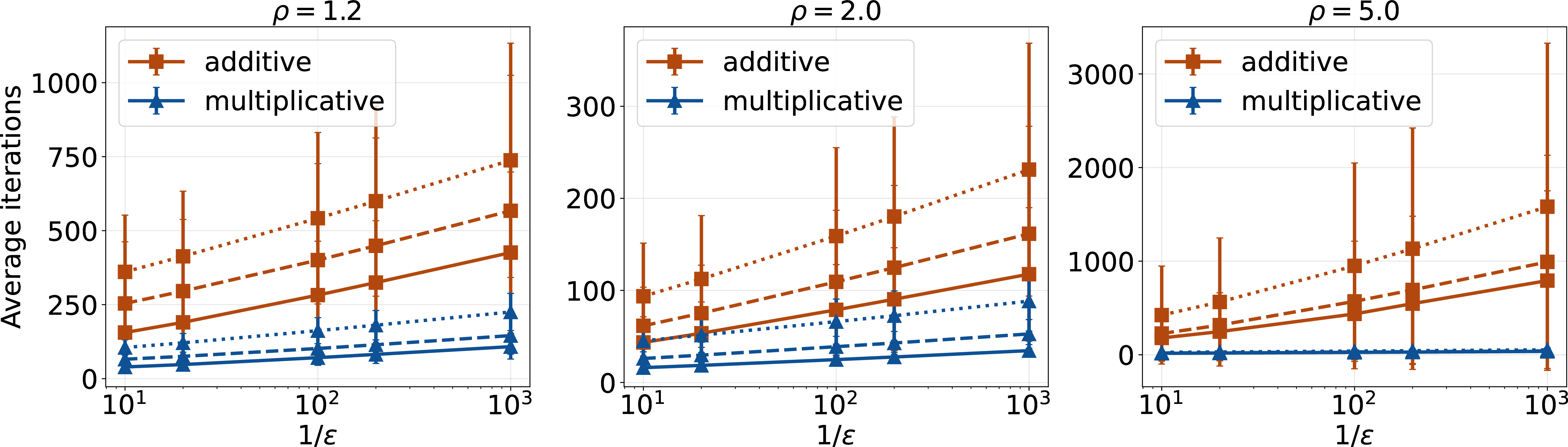
We conduct numerical experiments on three types of datasets: Spliddit instances, AAMAS bidding instances, and synthetic instances. For each type, we test three convex CES disutilities with \(\rho \in \{1.2, \;2, \;5\}\). We compare the number of iterations required to compute an \(\varepsilon\)-approximate equilibrium, where \(\varepsilon \in \{0.1, \;0.05, \;0.01, \;0.005, \;0.001\}\). The experiments were implemented on a personal desktop with Apple M1 chip.

5.0.0.1 Spliddit instances.

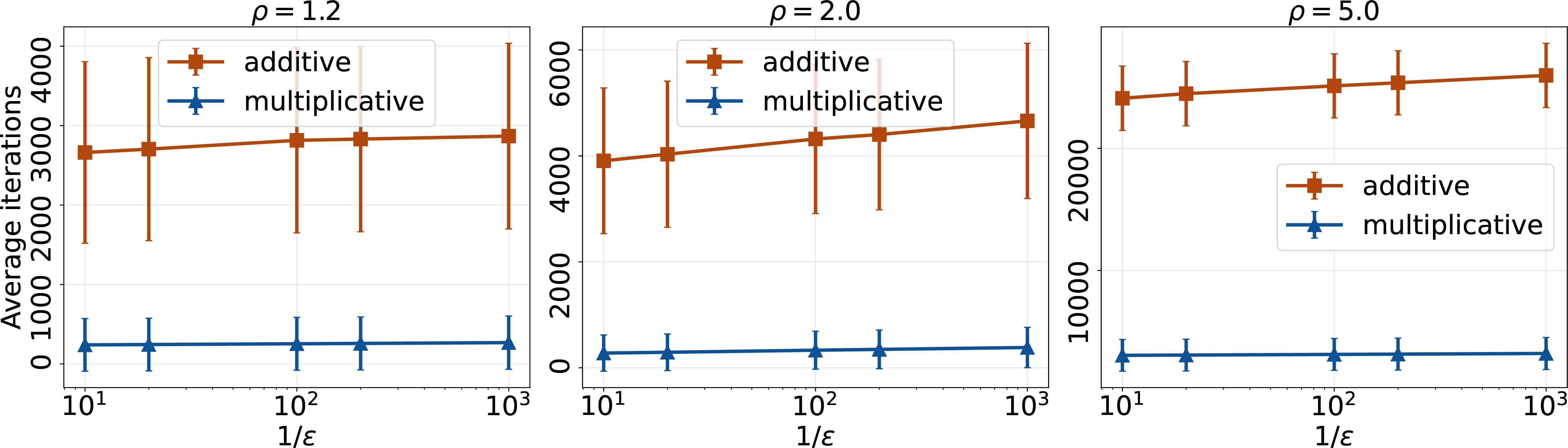
Spliddit is a research-driven online platform that helps users divide resources fairly and transparently [36]. We use a dataset containing \(670\) task-distribution instances from Spliddit. The instance sizes range from \(2\) to \(6\) agents and from \(2\) to \(37\) tasks. We test all instances in the dataset and report the average number of iterations across different approximation tolerances \(\varepsilon\) in 1.

We use the following heuristic to select practical stepsizes for both algorithms. For each instance, we start with a large stepsize and iteratively search for an upper bound on the admissible stepsizes. If a trajectory leaves the price simplex, we set the current stepsize as an upper bound on the admissible range. We then perform a grid search (excluding the stepsize upper bound) over the admissible range using \(9\) grid points, from the largest to the smallest. If all tested stepsizes are admissible, we choose the one that achieves the best performance, measured by the smallest approximation tolerance. We also use this method to select practical stepsizes for other types of instances.

5.0.0.2 AAMAS bidding instances.

We construct a set of AAMAS bidding instances from a dataset of bids submitted by PC members at the AAMAS conference for potential papers to review. This dataset is obtained from PrefLib [37] and is also used by [16]. We convert reviewer bids into a disutility matrix using the mapping yes:1, maybe:3, missing:5, no:7, and conflict:1401. For each instance, we choose a random seed paper, take its nearest 100 papers under the squared distance between bidding profiles, and then select the 200 reviewers with the most positive responses on this paper set. Finally, we optionally add Gaussian noise to the resulting 100\(\times\)200 disutility matrix. For each \(\rho\), we sample 10 such instances and set all reviewers’ budgets to one, as is standard in fair-division settings. 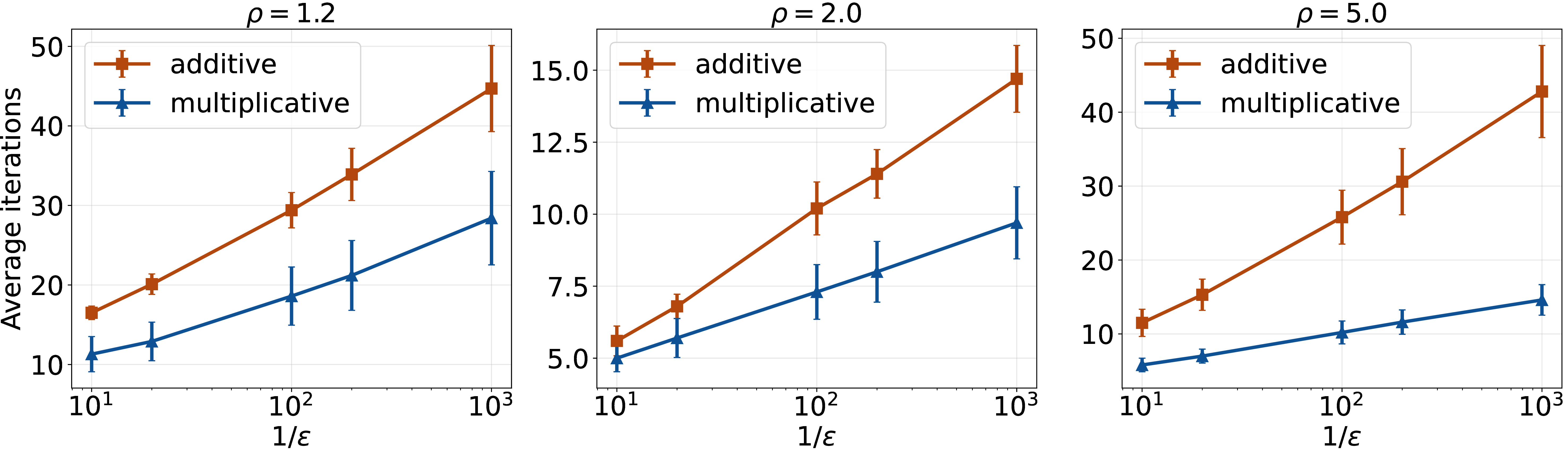The results are shown in 4.

5.0.0.3 Synthetic instances.

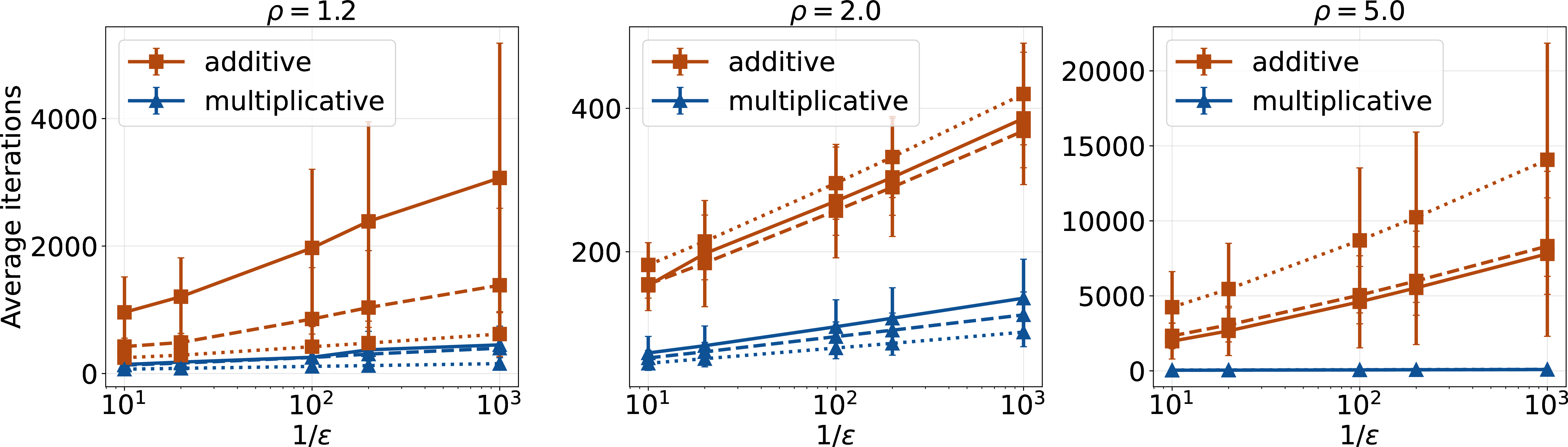
We simulate a set of large instances to compare the empirical convergence rates of the two dynamics. We generate instances with \(100\) agents and \({500,1000,2000}\) chores, reflecting the fact that, in many real applications, the number of chores is much larger than the number of agents. For each problem size, we test the dynamics on \(20\) instances generated from \(20\) random seeds. We consider two valuation distributions: (1) a lognormal distribution with location parameter \(0\) and scale parameter \(1\); and (2) a truncated normal distribution with mean \(0.5\) and standard deviation \(0.2\), truncated below at \(0.01\). We set each agent’s budget to one. The results are shown in 2 5.

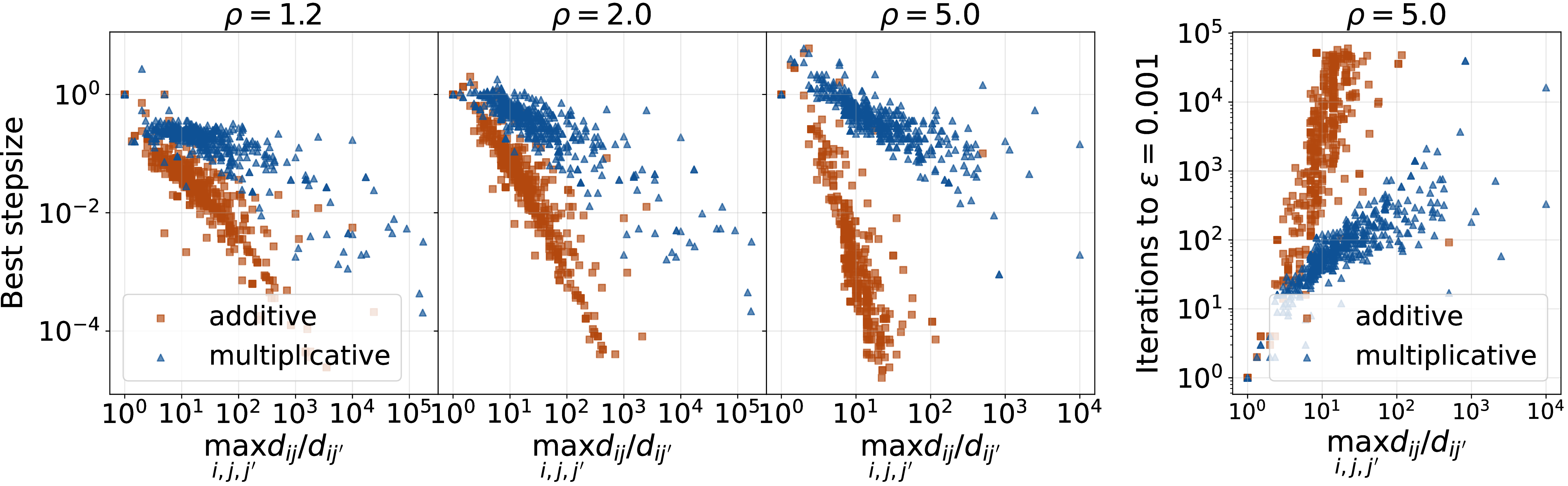
5.0.0.4 Discussions.

Overall, multiplicative tâtonnement significantly outperforms relative tâtonnement. On Spliddit instances, multiplicative tâtonnement requires fewer than \(100\) iterations to find a \(0.001\)-approximate CE, even when \(\rho = 5\). In contrast, relative tâtonnement may require a very large number of iterations to find an approximate CE, and this number increases as \(\rho\) grows. In particular, relative tâtonnement can take more than \(20{,}000\) iterations to find a \(0.1\)-approximate CE. On AMMAS bidding instances, although both dynamics compute approximate CE within \(100\) iterations, multiplicative tâtonnement still reduces the iteration cost by roughly half. These instances are relatively easy to solve because their value sets are sparse, containing only \(5\) distinct values. On synthetic instances, multiplicative tâtonnement typically achieves a \(10\times\) speedup, even for small values of \(\rho\).

An interesting observation is the relationship between the best practical stepsizes and the maximum value ratio \(\max_{i,j,j'} d_{ij}/d_{ij'}\). We illustrate this relationship based on the Spliddit instances with scatter plots in 3. The plots reveal a clear pattern: as \(\max_{i,j,j'} d_{ij}/d_{ij'}\) increases, the best stepsize decreases at a rate consistent with our analysis. In particular, the largest admissible stepsize appears to be inversely proportional to \((\max_{i,j,j'} d_{ij}/d_{ij'})^\rho\). This relationship becomes linear on a log-log plot, where the slope reflects the exponent. As shown in the three plots on the left, the slopes for relative tâtonnement are approximately \(1.2\), \(2\), and \(5\), respectively. In contrast, the slope for multiplicative tâtonnement changes only mildly.

Additionally, from the right plot in 3, as \(\max_{i, j, j'} d_{ij} / d_{ij'}\) increases, the increase of the number of iterations appearantly has a separation between two dynamics: the iteration cost of multiplicative tâtonnement dynamics scale up at a \(\tfrac{1}{2}\) rate of that of relative tâtonnement, which also matches our theoretical results as \(\rho \rightarrow \infty\) and thus \(\sigma \rightarrow 1\): multiplicative tâtonnement has a dependency \((d_{\min})^{-1} + (d_{\min})^{-\sigma}\) and relative tâtonnement has a dependency \((d_{\min})^{-1-\sigma}\).

Acknowledgments↩︎

The research of Bhaskar Ray Chaudhury was supported by NSF CAREER Grant CCF-2441580. The research of Christian Kroer was supported by the Office of Naval Research awards N00014-22-1-2530 and N00014-23-1-2374, and the National Science Foundation awards IIS-2147361 and IIS-2238960. The research of Ruta Mehta was supported by NSF Grant CCF-2334461.

6 Additional related work↩︎

Computation of CE in Fisher markets. A series of foundational works established convex programming and linear complementarity problem (LCP) characterizations of the CE set across various economic models [21], [38], [39]. Building on these formulations, [40] obtained the first strongly polynomial-time algorithm in this setting. Subsequent research has produced a diverse body of algorithms for computing CE in broader market models—such as exchange and Arrow-Debreu markets—going well beyond the linear Fisher case [41]–[44]. These include interior point methods [45], [46], as well as combinatorial approaches [47]. For CES markets specifically, polynomial-time computation has been established under various restrictions, including weak gross substitutes regimes (\(\sigma > 1\)) [6], [8], fixed numbers of agents or goods [48], and more general homothetic utilities via convex programming [49]. In the chores market, a separate line of work has yielded polynomial-time algorithms achieving arbitrarily good approximations of CE [13], [14], [16]. More recently, [15] gave a polynomial-time algorithm for exactly computing a CE in linear chores Fisher markets whenever the number of agents or chores is constant.

7 Proofs of 2↩︎

8 Proofs in 3↩︎

We repeat the definition of \(\ell_0\) (for all disutility functions satisfying 2) here: \[\ell_0 = \frac{1}{3m} \min_{i} \left\{ \underset{j, j' \in [m]}{\min_{\tilde{\mathbf{x}}_i \geq 0, \mathbf{d}'_i > 0, }} \left\{ \frac{d'_{ij}}{d'_{ij'}}\;\left| \;{j, j' \in [m]}, \tilde{x}_{ij} \geq \frac{1}{2 n m}, \tilde{x}_{ij'} \leq 2m B_i, \mathbf{d}'_i \in \partial d_i(\tilde{\mathbf{x}}_i) \right. \right\} \right\} > 0.\]

For CES disutility function with \(\rho \in (1, \infty)\), i.e., \(d_i(\mathbf{x}_i) = (\sum_{j=1}^m (d_{ij} x_{ij})^\rho)^{1/\rho}\), then one can show that \[\ell_0 = \frac{1}{3m} \min_{i \in [n]} \left\{ \min_{j, j' \in [m]} \left(\frac{d_{ij}}{d_{ij'}}\right)^\rho \left( \frac{\norm*{\mathbf{B}}_1}{4 n m^2 B_i} \right)^{\rho - 1} \right\} > 0. \label{eq:nui32defn32CES}\tag{9}\] The quantity \(\ell_0\) is useful in the proof as the excess supply is positive whenever a price is lower than \(\ell_0\), which is shown by [1].

Leveraging this sharper boundedness of the excess demand, we can show that, the desired behaviors of the discrete-time multiplicative tâtonnement holds with a larger stepsize than a naïve bound. Moreover, this admissible stepsize will not blow up when \(\rho \rightarrow \infty\).

We restate 2 here for reference.

9 Proofs of 4↩︎

9.1 Details on the rate of relative tâtonnement↩︎

Here, we focus on the case where each convex CES disutility functions are with \(\rho > 2\). Note that we use a different parameterization (\(d_i(\mathbf{x}_i) = (\sum_{j = 1}^m (d_{ij} x_{ij})^\rho)^{1/\rho}\)) for the convex CES disutility functions from that in [1] (\(d_i(\mathbf{x}_i) = (\sum_{j = 1}^m d_{ij} x_{ij}^\rho)^{1/\rho}\)).

We consider the terms with \(1/\ell_0\) and lower bound all other nonnegative terms in the expression of the smoothness modulus. In their Lemma 15, \(r_i\) can equal \(1\) in our setting (by 1), then we have \[\begin{align} L \geq \sum_{i=1}^n B_i R_i L_i &\geq \sum_{i=1}^n B_i R_i ((\sigma - 1)\frac{(\max_j d_{ij}^\rho)^{\frac{(\sigma - 1)^2}{\sigma}}}{(\min_j d_{ij}^\rho)^{\sigma - 1}}) \frac{1}{2\ell_0} \\ &= \sum_{i=1}^n B_i (\min_j d_{ij}^\rho)^{-1/\rho} ((\sigma - 1)\frac{(\max_j d_{ij}^\rho)^{\frac{(\sigma - 1)^2}{\sigma}}}{(\min_j d_{ij}^\rho)^{\sigma - 1}}) \frac{1}{2\ell_0}. \end{align}\]

Since we have \(d_i(\mathbf{1}_m) = 1\) by 1, we have \[\max_{j} d_{ij}^\rho \geq \frac{1}{m}\sum_{j = 1}^m d_{ij}^\rho = \frac{1}{m}.\] Therefore, \[L \geq \sum_{i=1}^n B_i (\min_j d_{ij})^{-1} ((\sigma - 1)\frac{1}{m^{\frac{(\sigma - 1)^2}{\sigma}}(\min_j d_{ij}^\rho)^{\sigma - 1}}) \frac{1}{2\ell_0}.\] Since \(\rho (\sigma - 1) = \rho (\frac{\rho}{\rho - 1} - 1) = \rho \frac{1}{\rho - 1} = \sigma\), and \(\frac{(\sigma - 1)^2}{\sigma} = \frac{1}{\rho(\rho - 1)} \leq \frac{1}{2}\), we have \[L \geq (\sigma - 1) m^{-\frac{1}{2}} (\min_j d_{ij})^{-(\sigma + 1)} \frac{1}{2\ell_0}.\] Since we can take \(\eta = \frac{1}{L}\), and their convergence guarantee leads to \(\lceil 2L(f(\mathbf{p}^0) - \underline{f}) / \varepsilon^2 \rceil\) iterations required to compute an \(\varepsilon\)-approximate CE.

The following lemma shows that \(f(\mathbf{p}^0) - \underline{f}\) is always bounded by a number that is polynomial in problem parameters.

10 Additional numerical experiments↩︎

References↩︎

---

1. \(\partial f(\mathbf{p}^k)\) denotes Clarke differential of function \(f\) at \(\mathbf{p}^k\).↩︎

2. We do not consider price projection, since it would require each chore manager to have access to the prices of other chores.↩︎

3. \(\partial f(\mathbf{p}^k)\) denotes Clarke differential of function \(f\) at \(\mathbf{p}^k\).↩︎