Multi-Hypothesis Test-Time Adaptation to Mitigate Underspecification
June 30, 2026
Abstract
Test-Time Adaptation (TTA) seeks to improve model robustness under distribution shifts by adapting parameters using unlabeled target data. However, in the absence of supervision, entropy-based adaptation is fundamentally underconstrained: multiple distinct parameter updates can achieve similarly low entropy while inducing drastically different decision boundaries. This phenomenon, known as underspecification, renders standard TTA brittle and prone to collapse into spurious modes. In this work, we reinterpret TTA through a posterior-inspired lens induced by entropy minimization, where low-entropy solutions define a pseudo-likelihood over parameters. Instead of committing to a single point estimate, we introduce a particle-based diversification framework that explores multiple plausible adaptation trajectories simultaneously. Our method can be viewed as a structured exploration of multiple plausible adaptation solutions, implemented through multi-level diversification at the output, parameter, optimizer, and input levels. Crucially, the framework acts as a plug-and-play wrapper compatible with existing TTA methods. Extensive experiments on challenging benchmarks demonstrate consistent gains in stability and robustness, achieving improvements of 3–4% under mixed shifts, 2–3% with batch size one, and 1–2.5% under label shifts, outperforming state-of-the-art baselines. Our results suggest that treating TTA as a multi-hypothesis inference problem, rather than a single-point optimization task, is key to mitigating underspecification and enabling reliable real-world deployment.
1 Introduction↩︎

Deep learning models have achieved remarkable performance across a range of tasks when training and test data are drawn from the same distribution. However, their performance often degrades sharply when deployed in the wild, where distribution shifts are inevitable [1], [2]. Test-time adaptation (TTA) has emerged as a promising strategy to bridge this train–test gap by adapting the model to the target distribution using only unlabeled test data [3]–[5].
Despite its appeal, standard TTA optimizes a single entropy-based objective in the absence of ground-truth supervision. This renders the adaptation process fundamentally underconstrained: multiple parameter configurations can achieve similarly low entropy on the target data while corresponding to qualitatively different decision boundaries. This phenomenon, underspecification, has been shown to induce instability and spurious feature reliance in deep models. From an optimization perspective, entropy minimization may admit multiple local minima of comparable value, yet these solutions need not generalize equally well under shift. We argue that existing TTA methods implicitly compute a single maximum a posteriori (MAP) solution under an entropy-induced pseudo-likelihood. In underspecified regimes, where multiple low-entropy configurations exist, such point-estimate adaptation is inherently unstable: small perturbations in optimization trajectory can lead to qualitatively different decision boundaries. Consequently, entropy minimization under shift should be viewed not as a well-posed optimization problem, but as a multi-hypothesis inference problem.
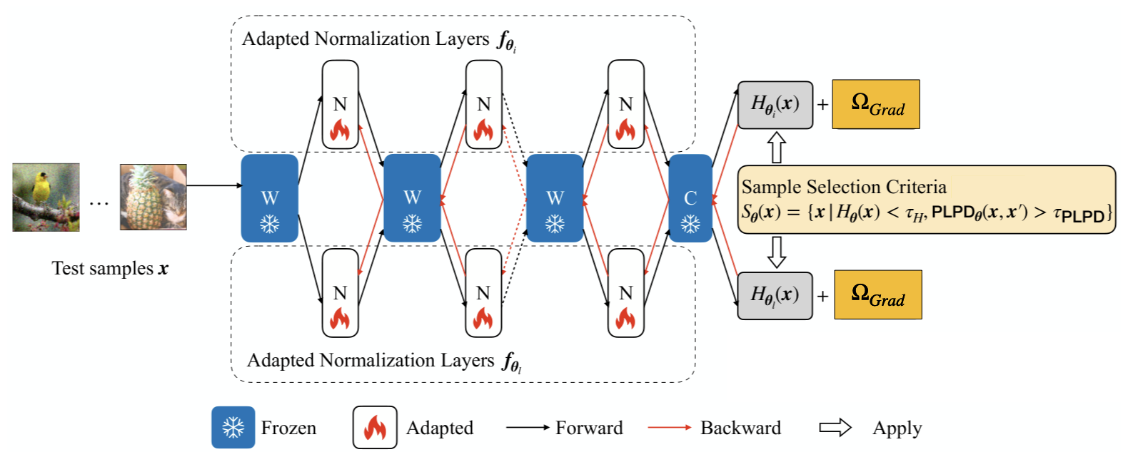
In this work, we reformulate TTA as a population-based inference problem and introduce a particle-driven diversification framework to approximate the posterior over adaptation parameters induced by entropy minimization. Rather than committing to a single entropy-minimizing trajectory, we maintain a population of interacting adaptation particles that explore distinct low-entropy regions of the parameter space while being regularized to prevent premature mode collapse. Each particle follows a unique optimization trajectory under entropy minimization, guided by multi-level diversification mechanisms that operate at the output, parameter, optimizer, and input levels. This perspective transforms TTA from a brittle point-estimation procedure into a controlled multi-trajectory exploration process. By preserving multiple plausible adaptation hypotheses and aggregating their predictions, our framework mitigates instability arising from underspecification and reduces reliance on spurious shortcuts. Importantly, the proposed approach is model-agnostic and acts as a plug-and-play wrapper that can enhance a broad class of existing TTA methods. We evaluate our framework on challenging benchmarks such as ImageNet-C [6] under mixed corruptions, label shifts, and batch size one settings. Across all scenarios, our method consistently improves robustness and stability, outperforming state-of-the-art TTA baselines by 1–4%. These results suggest that treating TTA as a multi-hypothesis inference problem is crucial for reliable deployment under distribution shift.
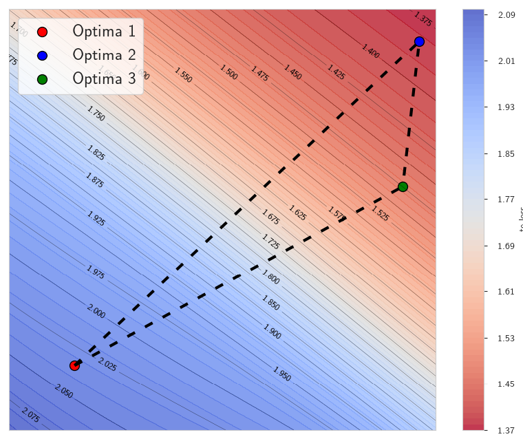
In 1, we illustrate the entropy landscape with respect to the model’s parameters \({\boldsymbol{\theta}}\) for a binary classification task. Suppose that \({\boldsymbol{\theta}}^0\) represents all parameters of the normalization layers in the source model. Without adaptation, the decision boundary is likely to be inadequate under Out-of-Distribtion (OOD) conditions. At test time, TTA approaches typically update the model by minimizing entropy to align target data with source data. Prior TTA approaches update \({\boldsymbol{\theta}}^0\) to either \({\boldsymbol{\theta}}_1\) or \({\boldsymbol{\theta}}_2\), optimizing the model toward low-entropy directions. Although these methods can improve overall performance, their decision boundaries remain suboptimal and can introduce additional errors. These issues are closely associated with the broader challenge of underspecification, which has been mitigated in other contexts using strategies such as data augmentation and ensembling. However, their integration into TTA remains largely unexplored. Although [7] indirectly used augmentation-based filtering to highlight robust features, this was not aimed at resolving underspecification itself. In contrast, our work directly tackles the root of underspecification by introducing a diversification-based adaptation framework that encourages representational diversity and enhances model robustness during TTA.
In this paper, we build on these observations to explain why existing TTA methods can be unreliable and to develop a more stable alternative. Specifically, starting from a source model with normalization parameters \({\boldsymbol{\theta}}^0\), we 1) initialize a collection of normalization parameter sets \(\Theta = \{{\boldsymbol{\theta}}_i\}_{i=1}^N\) from \({\boldsymbol{\theta}}^0\) while keeping all non-normalization layers frozen (see 2), 2) use \(N\) optimizers with distinct hyperparameters to adapt different particles \({\boldsymbol{\theta}}_i\), and 3) apply diversification regularization to prevent particle collapse. At inference time, we aggregate predictions from the \(N\) adapted parameter sets \(\{{\boldsymbol{\theta}}_i\}_{i=1}^N\), thereby combining multiple plausible adaptation hypotheses instead of committing to a single adapted solution. Each \({\boldsymbol{\theta}}_i\) follows a distinct entropy-minimization trajectory, and their interaction encourages exploration of different low-entropy regions. Aggregating these interacting particles reduces sensitivity to spurious modes induced by underspecification. Empirically, this population-based inference consistently improves stability and robustness over single-model entropy minimization, outperforming representative TTA baselines including Tent [4], SAR [8], and DeYO [7].
Summary of Contributions:
We reinterpret entropy-based test-time adaptation as an implicit posterior inference problem under underspecification, highlighting the limitations of single-point MAP adaptation.
We propose a particle-based diversification framework that approximates posterior exploration over adaptation parameters through multi-level diversification (output, parameter, optimizer, and input levels).
We demonstrate that controlled particle interactions mitigate collapse into spurious modes and consistently improve robustness across mixed shifts, label shifts, and batch size one scenarios.
Extensive ablation studies reveal that gradient-based diversification provides the strongest stabilization effect, offering practical guidance for reliable test-time adaptation.
2 Preliminaries↩︎
2.1 Test Time Adaptation↩︎
Suppose that we have a training (source) dataset \({\mathcal{D}}^{s} = \{({\mathbf{x}}_j^{s}, y_j^{s})\}_{j=1}^{N^{s}}\) where \({\mathbf{x}}_j^{s} \in {\mathcal{X}}^{s}\) and \(y_j^{s} \in {\mathcal{Y}}^{s}\), \(N^{s}\) is the number of training instances, and a testing (target) set \({\mathcal{D}}^{t} = \{({\mathbf{x}}_j^{t}, y_j^{t})\}_{j=1}^{N^{t}}\) where \({\mathbf{x}}_j^{t} \in {\mathcal{X}}^{t}\) and \(y_j^{t} \in {\mathcal{Y}}^{t}\), \(N^{t}\) is the number of test instances. A source model \({\boldsymbol{f}}_{{\boldsymbol{\theta}}}(\cdot)\) with parameters \({\boldsymbol{\theta}}\) is first trained on \({\mathcal{D}}^{s}\) and then evaluated on \({\mathcal{D}}^{t}\). When \({\mathcal{D}}^{t}\) involves OOD, \({\boldsymbol{f}}_{{\boldsymbol{\theta}}}(\cdot)\) may not generalize well. Test Time Adaptation approaches adapt the model \({\boldsymbol{f}}_{{\boldsymbol{\theta}}}(\cdot)\) on the target dataset \({\mathcal{D}}^{t} = \{{\mathbf{x}}_j^{t}\}_{j=1}^{N^{t}}\) without any labels, since labels \(y_j^{t}\) are not accessible at test time. In this paper, we focus on TTA approaches that only reuse the normalization layers of the source model; therefore, without loss of generality, we use \({\boldsymbol{\theta}}\) to represent all parameters of the normalization layers.
2.2 Entropy Minimization↩︎
Without the need for additional labeled data, previous TTA methods [4], [8] utilize the entropy of model predictions as the objective function to adapt the model \({\boldsymbol{f}}_{{\boldsymbol{\theta}}}(\cdot)\): \[\min H_{\boldsymbol{\theta}}({\mathcal{X}}^{t}) = \min \sum^{N^{t}}_{j} H({\boldsymbol{f}}_{{\boldsymbol{\theta}}} ({\mathbf{x}}_j^{t})), \label{eq:entropy32minimization}\tag{1}\] where \(H_{\boldsymbol{\theta}}(\cdot)\) is entropy and measured by the Shannon entropy [9]: \[H_{\boldsymbol{\theta}}({\mathbf{x}}) = -{\mathbf{p}}_{\boldsymbol{\theta}}({\mathbf{x}}) \cdot \log {\mathbf{p}}_{\boldsymbol{\theta}}({\mathbf{x}}) = - \sum^{C}_{c} p_{\boldsymbol{\theta}}(x)_c \log p_{\boldsymbol{\theta}}(x)_c, \label{eq:entropy}\tag{2}\] where \({\mathbf{p}}_{\boldsymbol{\theta}}({\mathbf{x}}) = \mathrm{softmax}({\boldsymbol{f}}_{{\boldsymbol{\theta}}}({\mathbf{x}})) = (p_{\boldsymbol{\theta}}(x)_1, ..., p_{\boldsymbol{\theta}}(x)_C)\), \(C\) is the number of class labels for the underlying classification task. Entropy is an unsupervised objective since it only depends on the model predictions instead of annotations.
2.3 Benchmark Methods and Datasets↩︎
For comparison, we conducted experiments on several benchmark datasets: 1) The ImageNet-C [10] benchmark consists of 15 diverse corruption types encompassing 5 severity levels for each type applied to validation images of ImageNet. 2) CIFAR-10-C and CIFAR-100-C [10] benchmarks provide the same 15 corruption types as ImageNet-C, but all images are derived from CIFAR-10 and CIFAR-100, respectively. We applied our method to mild scenarios proposed by [4] and wild scenarios proposed by [8]. The mild scenario is to adapt models with a batch of test samples that have the same distribution shift type and randomly shuffled label distribution. In contrast, the wild scenario includes three more realistic settings: a) dynamic shifts in the ground-truth test label distribution, which lead to class imbalance at each corruption, b) batch size equal to one (single-sample adaptation), and c) mixtures of multiple distribution shifts. We evaluate three representative test time adaptation baseline methods including Tent [4], SAR [8] and DeYO [7], and employ ResNet-50-GN (group normalization) and ViTBase-LN (layer normalization) [11] for ImageNet-C, CLIP-VitBase-Patch32-LN [12] for CIFAR-10-C and CIFAR-100-C, taking into consideration test time adaptation’s utilization across various normalization layers. To further assess robustness under broader distribution shifts, we additionally evaluate on ColoredMNIST, Waterbirds, ImageNet-R [13], and VisDA-2021 [14], which capture spurious correlations and domain shifts beyond corruption-based benchmarks. Detailed results are provided in Appendix 8.
3 Methodology and Results↩︎
| Seed | Final Entropy \(\downarrow\) | Acc. (%) \(\uparrow\) | \(\|\theta^{\mathrm{final}}-\theta^{0}\|_2\) | Mean Pairwise \(\|\Delta \theta\|_2\) |
|---|---|---|---|---|
| 0 | 0.247 | 45.1 | 0.92 | 0.51 |
| 1 | 0.241 | 34.6 | 0.88 | 0.47 |
| 2 | 0.245 | 41.8 | 0.95 | 0.54 |
| 3 | 0.249 | 32.9 | 0.90 | 0.49 |
| 4 | 0.244 | 37.5 | 0.93 | 0.52 |
| Mean \(\pm\) Std | 0.245 \(\pm\) 0.003 | 38.37 \(\pm\) 4.80 | 0.92 \(\pm\) 0.03 | 0.51 \(\pm\) 0.03 |
6pt
Prior TTA approaches adapt a single model at test time by minimizing an unsupervised objective, most commonly, prediction entropy [4], or by combining entropy minimization with augmentation-based filtering [7], [15], [16]. While these strategies have demonstrated promising improvements under distribution shift, they rely on updating a single parameter instance in the absence of supervision. As discussed in 1, entropy minimization is inherently underconstrained: multiple parameter configurations can achieve similar low entropy while corresponding to qualitatively different decision boundaries. Updating a single model therefore risks drifting toward suboptimal low-entropy solutions, amplifying simplicity bias and accumulating adaptation errors over time.
To empirically evaluate the stability of single-model entropy-based adaptation, we run DeYO [7] under the batch size \(1\) protocol multiple times with different random seeds while keeping the hyperparameters fixed. 1 shows that the final entropy values are nearly identical across runs (\(0.245 \pm 0.003\)), yet the resulting accuracies vary substantially (\(38.37 \pm 4.80\)%). Furthermore, the adapted normalization parameters converge to different endpoints in parameter space. In particular, \(\|\boldsymbol{\theta}^{\mathrm{final}}-\boldsymbol{\theta}^{0}\|_2\) measures the magnitude of the parameter change from the source model, while the mean pairwise distance \(\|\Delta\boldsymbol{\theta}\|_2\) denotes the average \(\ell_2\) distance between final parameter vectors obtained from different seeds (computed across all seed pairs). These results indicate that entropy minimization does not uniquely specify a robust adaptation outcome: multiple low-entropy solutions correspond to qualitatively different decision boundaries and generalization performance. This instability highlights the need for structured mechanisms that explicitly maintain diverse adaptation hypotheses. To address this limitation, we adopt a population-based formulation of test-time adaptation. Instead of committing to a single adaptation trajectory, we maintain a collection of \(K\) interacting adaptation particles \[\Theta = \{\theta_i\}_{i=1}^{K},\] where each \(\theta_i\) represents the normalization parameters adapted from the shared source model \(\theta^0\). All non-normalization layers remain frozen and shared across particles, following standard TTA practice [4], [7], [8]. Each particle is initialized from \(\theta^0\) and adapted online on the target stream. We define the general population adaptation objective as \[\mathcal{L}(X) = \frac{1}{K} \sum_{i=1}^{K} \ell(X; \theta_i) + \lambda\,\Omega(\Theta), \label{eq:pop95objective}\tag{3}\] where \(\ell(X; \theta_i)\) denotes the entropy-based adaptation loss for particle \(i\) (Eq. 1 ), and \(\Omega(\Theta)\) is a diversification regularizer that prevents premature particle collapse. The key idea is to encourage controlled exploration of multiple low-entropy regions in parameter space while maintaining interaction between particles. Unlike naive ensembling, where models are trained independently and averaged post hoc, our formulation explicitly couples particle dynamics during adaptation. Diversification therefore acts not as a static aggregation trick, but as a mechanism for mitigating underspecification during optimization.
We instantiate \(\Omega(\Theta)\) through complementary diversification mechanisms operating at multiple levels: output-level, parameter-level, optimizer-level, and input-level. Each mechanism targets a distinct failure mode of single-model entropy minimization under distribution shift, as detailed below.
3.1 Output-level Diversification↩︎
Output-level diversification promotes disagreement among particles at the prediction level, preventing premature collapse to identical predictive hypotheses under entropy minimization. Let \(p_i(X)\) denote the predictive distribution of particle \(\theta_i\) on input batch \(X\). To encourage predictive diversity, we maximize pairwise divergence between particle outputs. We define the output-level regularizer as: \[\Omega_{\mathrm{KL}}(\Theta) = - \frac{1}{K(K-1)} \sum_{i \neq j} D_{\mathrm{KL}}\!\left( p_i(X) \,\|\, p_j(X) \right), \label{eq:kl95div}\tag{4}\] where \(D_{\mathrm{KL}}(\cdot \| \cdot)\) denotes the Kullback–Leibler divergence. The negative sign ensures that minimizing the overall objective in 3 increases predictive divergence between particles. This repulsive interaction encourages particles to occupy distinct low-entropy regions of the solution space, thereby reducing the risk of collective collapse into the same spurious decision boundary. Unlike naive ensembling, where models are trained independently and averaged post hoc, our formulation explicitly couples particle dynamics during adaptation, allowing disagreement to emerge as a controlled exploration mechanism. While naive ensembling already improves robustness over single-model adaptation, we empirically observe that independently trained particles tend to converge toward similar adaptation trajectories under entropy minimization. This trajectory alignment limits the diversity benefits of simple averaging. The proposed diversification mechanisms explicitly prevent such collapse and yield consistent gains beyond naive ensembling.
3.2 Parameter-level Diversification↩︎
3.2.1 Stein Variational Gradient Descent [17]: To further promote structured exploration of multiple adaptation hypotheses, we employ Stein Variational Gradient Descent (SVGD) as a particle interaction mechanism. Unlike standard gradient descent that converges to a single solution, SVGD evolves a set of particles jointly to approximate a target distribution through deterministic updates with repulsive interactions. We define a pseudo-posterior over normalization parameters as \[\tilde{p}(\theta) \propto \exp\!\left(- \ell(X; \theta)\right) \exp\!\left(-\frac{\gamma}{2} \|\theta - \theta^0\|_2^2 \right),\] where \(\ell(X; \theta)\) is the entropy adaptation loss (Eq. 1 ). The second exponential term acts as an implicit Gaussian prior centered at the source normalization parameters \(\theta^0\), discouraging excessive drift during adaptation. The coefficient \(\gamma > 0\) controls the strength of this quadratic anchoring term, balancing adaptation flexibility and retention of source-domain inductive bias. SVGD updates each particle \(\theta_i\) according to \[\theta_i \leftarrow \theta_i + \epsilon \, \phi(\theta_i),\] where \(\epsilon > 0\) is the particle update step size, and \[\phi(\theta_i) = \frac{1}{K} \sum_{j=1}^{K} \left[ \kappa(\theta_j, \theta_i)\, \nabla_{\theta_j} \log \tilde{p}(\theta_j) + \nabla_{\theta_j} \kappa(\theta_j, \theta_i) \right].\]
Here, \(K\) denotes the number of particles and \(\kappa(\cdot,\cdot)\) is a positive-definite kernel (e.g., an RBF kernel) that induces repulsive interactions between particles. The first term drives particles toward low-entropy regions of the adaptation objective, while the second term prevents collapse by encouraging dispersion in parameter space. In the context of test-time adaptation, this joint update enables particles to explore multiple plausible low-entropy solutions, thereby mitigating underspecification and reducing sensitivity to spurious adaptation modes.
3.2.2 Gradient-based Diversification: To mitigate simplicity bias during test-time adaptation, we promote functional diversity by encouraging particles to respond differently to input perturbations. Instead of enforcing parameter-space separation alone, we directly regularize the alignment of input gradients across particles. For particle \(\theta_i\), let \[g_i = \nabla_X \ell(X; \theta_i)\] denote the gradient of the entropy loss with respect to the input batch \(X\). We define the gradient-based diversification term as \[\Omega_{\mathrm{Grad}}(\Theta) = - \frac{1}{K(K-1)} \sum_{i \neq j} \langle g_i, g_j \rangle, \label{eq:grad95div}\tag{5}\] where \(\langle \cdot , \cdot \rangle\) denotes the Euclidean inner product. Minimizing the overall objective in Eq. 3 therefore penalizes large positive gradient alignment between particles. This encourages particles to rely on different input directions during adaptation, promoting diverse decision boundaries under distribution shift. Unlike output-level disagreement, which acts on predictions, or parameter-space repulsion, which operates directly in weight space, gradient-based diversification regularizes the functional behavior of particles. By reducing gradient alignment, particles are discouraged from collapsing toward identical adaptation trajectories, thereby improving robustness in underspecified settings. We thoroughly investigate output-level and parameter-level diversification under wild settings; results for mild settings are provided in Appendix 11.
| Noise | Blur | Weather | Digital | |||||||||||||
| Batch Size 1 | Gauss. | Shot | Impl. | Defoc. | Glass | Motion | Zoom | Snow | Frost | Fog | Brit. | Contr. | Elastic | Pixel | JPEG | Avg. |
| ResNet-50-GN | 18.01 | 19.78 | 17.91 | 19.80 | 11.41 | 21.39 | 24.90 | 40.41 | 47.29 | 33.60 | 69.31 | 36.31 | 18.59 | 28.41 | 52.29 | 30.60 |
| Tent | 28.85\(\pm\)0.4 | 35.95\(\pm\)0.3 | 33.49\(\pm\)0.3 | 16.67\(\pm\)0.2 | 7.19\(\pm\)0.3 | 27.35\(\pm\)0.3 | 30.14\(\pm\)0.4 | 17.97\(\pm\)0.2 | 25.20\(\pm\)0.2 | 2.27\(\pm\)0.2 | 71.88\(\pm\)0.1 | 46.24\(\pm\)0.1 | 7.36\(\pm\)0.3 | 52.72\(\pm\)0.3 | 56.40\(\pm\)0.1 | 30.65 |
| SAR | 28.51\(\pm\)0.3 | 30.91\(\pm\)0.4 | 29.27\(\pm\)0.1 | 18.50\(\pm\)0.1 | 15.34\(\pm\)0.3 | 28.80\(\pm\)0.3 | 30.53\(\pm\)0.2 | 44.47\(\pm\)0.3 | 44.27\(\pm\)0.2 | 32.94\(\pm\)0.6 | 72.03\(\pm\)0.2 | 44.67\(\pm\)0.1 | 13.16\(\pm\)2.8 | 47.70\(\pm\)0.1 | 56.23\(\pm\)0.1 | 35.82 |
| 41.97\(\pm\)0.7 | 44.21\(\pm\)0.4 | 43.03\(\pm\)0.7 | 21.81\(\pm\)0.1 | 23.28\(\pm\)0.3 | 40.87\(\pm\)0.1 | 26.10\(\pm\)4.3 | 53.24\(\pm\)0.2 | 51.22\(\pm\)0.2 | 35.13\(\pm\)6.1 | 72.39\(\pm\)0.1 | 52.50\(\pm\)0.2 | 42.44\(\pm\)0.3 | 59.10\(\pm\)0.0 | 58.73\(\pm\)0.1 | 44.40 | |
| 42.54\(\pm\)0.4 | 44.95\(\pm\)0.3 | 43.61\(\pm\)0.4 | 22.47\(\pm\)0.1 | 23.97\(\pm\)0.2 | 41.00\(\pm\)0.1 | 30.90\(\pm\)0.3 | 53.70\(\pm\)0.2 | 51.66\(\pm\)0.1 | 27.93\(\pm\)0.2 | 73.37\(\pm\)0.3 | 52.89\(\pm\)0.1 | 47.01\(\pm\)0.2 | 59.66\(\pm\)0.0 | 59.53\(\pm\)0.1 | 45.01 | |
| 42.57\(\pm\)0.3 | 44.90\(\pm\)0.3 | 43.79\(\pm\)0.3 | 22.72\(\pm\)0.1 | 24.20\(\pm\)0.2 | 40.89\(\pm\)0.1 | 32.04\(\pm\)0.3 | 53.40\(\pm\)0.1 | 51.69\(\pm\)0.1 | 28.41\(\pm\)0.1 | 73.34\(\pm\)0.0 | 53.00\(\pm\)0.1 | 46.39\(\pm\)0.1 | 59.64\(\pm\)0.1 | 59.62\(\pm\)0.1 | 45.11 | |
| 42.50\(\pm\)0.2 | 44.74\(\pm\)0.2 | 43.70\(\pm\)0.3 | 22.50\(\pm\)0.1 | 24.06\(\pm\)0.2 | 40.77\(\pm\)0.1 | 35.05\(\pm\)0.2 | 53.67\(\pm\)0.1 | 51.80\(\pm\)0.2 | 32.44\(\pm\)0.1 | 73.33\(\pm\)0.0 | 52.97\(\pm\)0.1 | 47.02\(\pm\)0.2 | 59.55\(\pm\)0.1 | 59.58\(\pm\)0.1 | 45.58 | |
| 42.73\(\pm\)0.2 | 44.99\(\pm\)0.2 | 43.88\(\pm\)0.2 | 22.49\(\pm\)0.1 | 24.32\(\pm\)0.1 | 41.07\(\pm\)0.1 | 25.63\(\pm\)0.2 | 54.10\(\pm\)0.1 | 52.03\(\pm\)0.0 | 58.88\(\pm\)0.1 | 73.33\(\pm\)0.1 | 53.28\(\pm\)0.1 | 47.69\(\pm\)0.2 | 59.41\(\pm\)0.1 | 59.70\(\pm\)0.0 | 46.90 | |
| VitBase-LN | 9.51 | 6.70 | 8.21 | 28.88 | 23.40 | 33.91 | 27.11 | 15.90 | 26.48 | 47.20 | 54.70 | 44.11 | 30.51 | 44.50 | 47.81 | 29.91 |
| Tent | 51.15\(\pm\)0.3 | 51.78\(\pm\)0.2 | 52.50\(\pm\)0.2 | 52.18\(\pm\)0.1 | 47.68\(\pm\)0.2 | 56.28\(\pm\)0.3 | 49.06\(\pm\)0.3 | 8.78\(\pm\)0.4 | 15.92\(\pm\)0.1 | 67.25\(\pm\)0.1 | 73.45\(\pm\)0.2 | 66.64\(\pm\)0.3 | 52.09\(\pm\)0.4 | 64.93\(\pm\)0.2 | 63.98\(\pm\)0.1 | 51.58 |
| SAR | 50.25\(\pm\)0.4 | 50.65\(\pm\)0.7 | 51.85\(\pm\)0.3 | 51.61\(\pm\)0.2 | 48.92\(\pm\)0.1 | 56.71\(\pm\)0.1 | 50.55\(\pm\)0.3 | 20.45\(\pm\)0.4 | 54.45\(\pm\)0.6 | 67.42\(\pm\)0.9 | 74.92\(\pm\)0.7 | 65.84\(\pm\)0.0 | 54.68\(\pm\)0.1 | 66.57\(\pm\)0.1 | 64.91\(\pm\)0.1 | 55.31 |
| 52.61\(\pm\)0.7 | 53.50\(\pm\)1.7 | 53.46\(\pm\)0.8 | 54.81\(\pm\)0.1 | 55.42\(\pm\)0.1 | 61.92\(\pm\)0.1 | 38.37\(\pm\)4.8 | 64.55\(\pm\)0.1 | 62.93\(\pm\)0.0 | 70.91\(\pm\)0.1 | 76.19\(\pm\)0.0 | 60.14\(\pm\)0.1 | 65.17\(\pm\)0.1 | 71.00\(\pm\)0.1 | 67.56\(\pm\)0.3 | 60.57 | |
| 53.47\(\pm\)0.3 | 54.67\(\pm\)0.2 | 54.80\(\pm\)0.4 | 56.17\(\pm\)0.2 | 56.51\(\pm\)0.1 | 62.18\(\pm\)0.1 | 47.20\(\pm\)0.3 | 64.91\(\pm\)0.3 | 63.04\(\pm\)0.1 | 70.97\(\pm\)0.1 | 76.64\(\pm\)0.1 | 66.20\(\pm\)0.1 | 66.10\(\pm\)0.1 | 71.42\(\pm\)0.1 | 68.29\(\pm\)0.3 | 62.17 | |
| 54.11\(\pm\)0.3 | 54.78\(\pm\)0.2 | 54.55\(\pm\)0.3 | 57.01\(\pm\)0.2 | 57.08\(\pm\)0.1 | 62.85\(\pm\)0.1 | 51.33\(\pm\)0.2 | 65.01\(\pm\)0.2 | 63.69\(\pm\)0.1 | 72.04\(\pm\)0.1 | 77.18\(\pm\)0.1 | 68.04\(\pm\)0.1 | 66.22\(\pm\)0.2 | 71.73\(\pm\)0.1 | 68.53\(\pm\)0.2 | 62.94 | |
| 54.83\(\pm\)0.3 | 55.78\(\pm\)0.3 | 55.97\(\pm\)0.2 | 56.46\(\pm\)0.3 | 56.84\(\pm\)0.2 | 62.66\(\pm\)0.2 | 54.78\(\pm\)0.2 | 65.05\(\pm\)0.1 | 63.69\(\pm\)0.2 | 72.30\(\pm\)0.2 | 77.24\(\pm\)0.1 | 68.04\(\pm\)0.1 | 66.00\(\pm\)0.0 | 71.82\(\pm\)0.1 | 68.89\(\pm\)0.2 | 63.36 | |
| 54.83\(\pm\)0.3 | 55.65\(\pm\)0.1 | 56.13\(\pm\)0.2 | 56.68\(\pm\)0.3 | 57.13\(\pm\)0.1 | 62.86\(\pm\)0.1 | 50.72\(\pm\)0.1 | 64.98\(\pm\)0.1 | 63.48\(\pm\)0.0 | 72.51\(\pm\)0.1 | 77.34\(\pm\)0.1 | 67.93\(\pm\)0.1 | 66.01\(\pm\)0.0 | 72.20\(\pm\)0.1 | 68.76\(\pm\)0.0 | 63.14 | |
| Noise | Blur | Weather | Digital | |||||||||||||
| Label Shifts | Gauss. | Shot | Impl. | Defoc. | Glass | Motion | Zoom | Snow | Frost | Fog | Brit. | Contr. | Elastic | Pixel | JPEG | Avg. |
| ResNet-50-GN | 17.9 | 19.9 | 17.9 | 19.7 | 11.3 | 21.3 | 24.9 | 40.4 | 47.4 | 33.6 | 69.2 | 36.3 | 18.7 | 28.4 | 52.2 | 30.6 |
| Tent | 1.67\(\pm\)0.2 | 2.02\(\pm\)0.2 | 2.01\(\pm\)0.1 | 12.17\(\pm\)0.3 | 2.14\(\pm\)0.3 | 23.00\(\pm\)0.2 | 13.74\(\pm\)0.4 | 8.86\(\pm\)0.2 | 13.69\(\pm\)0.2 | 1.00\(\pm\)0.1 | 73.00\(\pm\)0.3 | 48.44\(\pm\)0.3 | 3.51\(\pm\)0.2 | 54.90\(\pm\)0.2 | 57.18\(\pm\)0.3 | 21.15 |
| SAR | 28.71\(\pm\)0.1 | 31.19\(\pm\)0.4 | 29.39\(\pm\)0.9 | 18.52\(\pm\)0.4 | 15.10\(\pm\)1.2 | 28.71\(\pm\)0.5 | 29.84\(\pm\)3.5 | 42.86\(\pm\)2.6 | 44.33\(\pm\)0.4 | 35.32\(\pm\)0.9 | 72.07\(\pm\)0.1 | 44.65\(\pm\)0.2 | 14.40\(\pm\)1.9 | 47.04\(\pm\)0.5 | 56.22\(\pm\)0.1 | 35.89 |
| 40.27\(\pm\)0.5 | 43.58\(\pm\)0.2 | 41.75\(\pm\)0.3 | 22.42\(\pm\)0.0 | 22.69\(\pm\)0.2 | 40.93\(\pm\)0.2 | 14.63\(\pm\)2.3 | 53.19\(\pm\)0.4 | 51.78\(\pm\)0.5 | 1.03\(\pm\)0.2 | 72.89\(\pm\)0.1 | 52.93\(\pm\)0.2 | 47.81\(\pm\)1.2 | 59.48\(\pm\)0.0 | 59.30\(\pm\)0.1 | 41.65 | |
| 41.37\(\pm\)0.3 | 44.24\(\pm\)0.2 | 42.43\(\pm\)0.3 | 22.52\(\pm\)0.1 | 23.21\(\pm\)0.2 | 40.95\(\pm\)0.2 | 12.46\(\pm\)0.4 | 52.49\(\pm\)0.3 | 51.83\(\pm\)0.4 | 1.39\(\pm\)0.4 | 73.30\(\pm\)0.3 | 52.91\(\pm\)0.2 | 47.81\(\pm\)0.3 | 59.53\(\pm\)0.1 | 59.59\(\pm\)0.2 | 41.74 | |
| 42.43\(\pm\)0.3 | 44.82\(\pm\)0.3 | 43.66\(\pm\)0.3 | 22.98\(\pm\)0.1 | 23.54\(\pm\)0.2 | 40.74\(\pm\)0.2 | 17.55\(\pm\)0.3 | 53.11\(\pm\)0.3 | 51.97\(\pm\)0.2 | 4.31\(\pm\)0.3 | 73.51\(\pm\)0.3 | 52.97\(\pm\)0.2 | 46.82\(\pm\)0.2 | 59.38\(\pm\)0.1 | 59.58\(\pm\)0.2 | 42.49 | |
| 42.49\(\pm\)0.3 | 44.87\(\pm\)0.3 | 43.56\(\pm\)0.2 | 22.92\(\pm\)0.1 | 23.70\(\pm\)0.2 | 40.76\(\pm\)0.2 | 17.59\(\pm\)0.2 | 53.07\(\pm\)0.3 | 52.03\(\pm\)0.2 | 1.87\(\pm\)0.3 | 73.38\(\pm\)0.3 | 52.93\(\pm\)0.2 | 46.28\(\pm\)0.1 | 59.18\(\pm\)0.2 | 59.28\(\pm\)0.1 | 42.26 | |
| 42.42\(\pm\)0.2 | 44.80\(\pm\)0.2 | 43.64\(\pm\)0.2 | 22.95\(\pm\)0.1 | 23.59\(\pm\)0.2 | 40.79\(\pm\)0.1 | 17.53\(\pm\)0.1 | 53.09\(\pm\)0.1 | 51.97\(\pm\)0.0 | 15.79\(\pm\)0.1 | 73.50\(\pm\)0.1 | 53.00\(\pm\)0.2 | 46.92\(\pm\)0.0 | 59.41\(\pm\)0.1 | 59.61\(\pm\)0.0 | 43.27 | |
| ViTBase-LN | 9.42 | 6.73 | 8.32 | 29.11 | 23.41 | 34.03 | 27.01 | 15.80 | 26.30 | 47.41 | 54.72 | 43.90 | 30.50 | 44.5 | 47.6 | 29.9 |
| Tent | 53.41\(\pm\)0.2 | 53.16\(\pm\)0.2 | 54.36\(\pm\)0.3 | 54.34\(\pm\)0.4 | 52.46\(\pm\)0.4 | 58.74\(\pm\)0.6 | 52.83\(\pm\)0.2 | 4.29\(\pm\)0.2 | 7.04\(\pm\)0.1 | 69.46\(\pm\)0.3 | 74.92\(\pm\)0.3 | 67.42\(\pm\)0.4 | 59.97\(\pm\)0.2 | 67.89\(\pm\)0.2 | 66.13\(\pm\)0.1 | 53.10 |
| SAR | 51.90\(\pm\)0.4 | 51.47\(\pm\)0.7 | 53.02\(\pm\)0.3 | 51.69\(\pm\)0.2 | 48.57\(\pm\)0.1 | 56.55\(\pm\)0.1 | 50.62\(\pm\)0.3 | 26.45\(\pm\)0.4 | 54.29\(\pm\)0.6 | 68.00\(\pm\)0.9 | 74.28\(\pm\)0.7 | 65.65\(\pm\)0.0 | 55.44\(\pm\)0.1 | 66.68\(\pm\)0.1 | 65.07\(\pm\)0.0 | 55.98 |
| 53.92\(\pm\)0.3 | 54.86\(\pm\)0.7 | 55.08\(\pm\)0.4 | 54.78\(\pm\)0.1 | 55.70\(\pm\)0.2 | 61.63\(\pm\)0.1 | 53.34\(\pm\)0.2 | 64.31\(\pm\)0.4 | 63.10\(\pm\)1.1 | 70.75\(\pm\)0.3 | 76.81\(\pm\)0.1 | 65.90\(\pm\)0.3 | 65.60\(\pm\)0.3 | 71.65\(\pm\)0.2 | 68.10\(\pm\)0.2 | 62.37 | |
| 54.11\(\pm\)0.3 | 54.91\(\pm\)0.4 | 55.41\(\pm\)0.4 | 55.75\(\pm\)0.1 | 56.25\(\pm\)0.2 | 61.95\(\pm\)0.1 | 56.15\(\pm\)0.1 | 64.14\(\pm\)0.1 | 63.03\(\pm\)0.3 | 71.76\(\pm\)0.4 | 76.74\(\pm\)0.2 | 67.47\(\pm\)0.2 | 65.54\(\pm\)0.2 | 71.51\(\pm\)0.1 | 67.95\(\pm\)0.2 | 62.84 | |
| 54.59\(\pm\)0.3 | 55.41\(\pm\)0.3 | 55.94\(\pm\)0.3 | 56.17\(\pm\)0.1 | 56.77\(\pm\)0.2 | 62.50\(\pm\)0.1 | 56.22\(\pm\)0.1 | 64.63\(\pm\)0.2 | 63.46\(\pm\)0.3 | 72.32\(\pm\)0.3 | 77.25\(\pm\)0.2 | 67.54\(\pm\)0.2 | 65.98\(\pm\)0.2 | 71.98\(\pm\)0.1 | 68.55\(\pm\)0.1 | 63.29 | |
| 54.56\(\pm\)0.2 | 55.33\(\pm\)0.2 | 55.89\(\pm\)0.2 | 56.08\(\pm\)0.1 | 56.52\(\pm\)0.1 | 62.47\(\pm\)0.1 | 56.76\(\pm\)0.1 | 64.65\(\pm\)0.2 | 63.57\(\pm\)0.2 | 72.21\(\pm\)0.2 | 77.24\(\pm\)0.1 | 67.97\(\pm\)0.1 | 65.81\(\pm\)0.1 | 71.98\(\pm\)0.1 | 68.35\(\pm\)0.1 | 62.24 | |
| 54.52\(\pm\)0.2 | 55.37\(\pm\)0.1 | 55.89\(\pm\)0.1 | 56.09\(\pm\)0.1 | 56.74\(\pm\)0.0 | 62.47\(\pm\)0.1 | 57.31\(\pm\)0.1 | 64.63\(\pm\)0.0 | 63.55\(\pm\)0.2 | 72.36\(\pm\)0.1 | 77.23\(\pm\)0.1 | 67.80\(\pm\)0.0 | 65.92\(\pm\)0.1 | 72.01\(\pm\)0.0 | 68.52\(\pm\)0.1 | 63.36 | |
Comparison on Wild Scenario. We evaluate our population-based adaptation framework on ImageNet-C under three challenging wild settings: (1) batch size \(1\), (2) label distribution shift, and (3) mixed distribution shifts. Results are reported in ¿tbl:tab:imagenet-c? ¿tbl:tab:imagenet-c-mix-shift?.
1) Batch size 1. When adaptation is performed on a single test sample, entropy minimization becomes highly unstable due to the lack of batch statistics. Table ¿tbl:tab:imagenet-c? shows that simply maintaining multiple
normalization particles (Ens) already improves robustness over single-model adaptation. For ViTBase-LN, the ensemble setting improves average accuracy by 2.23% over DeYO, outperforming all baselines across most corruption types. ResNet-50-GN
exhibits similar gains.
Introducing explicit diversification further strengthens performance. Among all strategies, gradient-based diversification (Grad) achieves the best results, improving average accuracy by 3.21% for ViTBase-LN and 2.50% for ResNet-50-GN over
DeYO. Notably, under severe corruptions such as Fog, Grad attains the highest overall accuracy (58.88%), indicating improved stability under extreme underspecification.
2) Label Distribution Shift. Under infinite class imbalance ratio [8], entropy minimization is prone to reinforcing dominant classes.
The ensemble baseline (Ens) improves over DeYO by 0.47% on ViTBase-LN, suggesting that population-based adaptation mitigates collapse toward biased modes. Applying diversification further enhances robustness: Grad achieves
improvements of 0.99% (ViTBase-LN) and 1.62% (ResNet-50-GN) over DeYO. These gains indicate that gradient-level functional repulsion reduces overconfidence under skewed label distributions.
3) Mixed Distribution Shifts. We further evaluate performance on mixtures of 15 corruption types at severity level 5. As shown in ¿tbl:tab:imagenet-c-mix-shift?, gradient-based diversification consistently delivers the strongest
robustness. Compared with the best-performing baseline, Grad improves accuracy by 3% on ResNet-50-GN and 4.32% on ViTBase-LN. These results confirm that particle-level exploration combined with functional repulsion effectively stabilizes
adaptation under compound shifts.
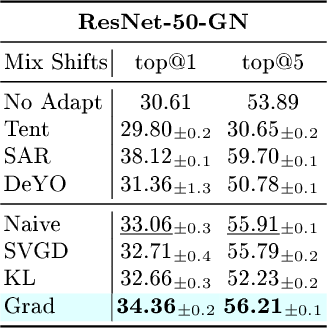
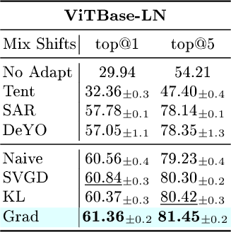
Overall, results across all wild scenarios demonstrate that (i) maintaining multiple adaptation particles already improves stability over single-model entropy minimization, and (ii) structured diversification, particularly gradient-based repulsion, provides additional robustness gains by preventing trajectory collapse under underspecified adaptation.
| Noise | Blur | Weather | Digital | |||||||||||||
| Batch Size 1 | Gauss. | Shot | Impl. | Defoc. | Glass | Motion | Zoom | Snow | Frost | Fog | Brit. | Contr. | Elastic | Pixel | JPEG | Avg. |
| VitBase-LN | 9.51 | 6.70 | 8.21 | 28.88 | 23.40 | 33.91 | 27.11 | 15.90 | 26.48 | 47.20 | 54.70 | 44.11 | 30.51 | 44.50 | 47.81 | 29.91 |
| Tent | 51.15\(\pm\)0.3 | 51.78\(\pm\)0.2 | 52.50\(\pm\)0.2 | 52.18\(\pm\)0.1 | 47.68\(\pm\)0.2 | 56.28\(\pm\)0.3 | 49.06\(\pm\)0.3 | 8.78\(\pm\)0.4 | 15.92\(\pm\)0.1 | 67.25\(\pm\)0.1 | 73.45\(\pm\)0.2 | 66.64\(\pm\)0.3 | 52.09\(\pm\)0.4 | 64.93\(\pm\)0.2 | 63.98\(\pm\)0.1 | 51.58 |
| SAR | 50.25\(\pm\)0.4 | 50.65\(\pm\)0.7 | 51.85\(\pm\)0.3 | 51.61\(\pm\)0.2 | 48.92\(\pm\)0.1 | 56.71\(\pm\)0.1 | 50.55\(\pm\)0.3 | 20.45\(\pm\)0.4 | 54.45\(\pm\)0.6 | 67.42\(\pm\)0.9 | 74.92\(\pm\)0.7 | 65.84\(\pm\)0.0 | 54.68\(\pm\)0.1 | 66.57\(\pm\)0.1 | 64.91\(\pm\)0.1 | 55.31 |
| 52.61\(\pm\)0.7 | 53.50\(\pm\)1.7 | 53.46\(\pm\)0.8 | 54.81\(\pm\)0.1 | 55.42\(\pm\)0.1 | 61.92\(\pm\)0.1 | 38.37\(\pm\)4.8 | 64.55\(\pm\)0.1 | 62.93\(\pm\)0.0 | 70.91\(\pm\)0.1 | 76.19\(\pm\)0.0 | 60.14\(\pm\)0.1 | 65.17\(\pm\)0.1 | 71.00\(\pm\)0.1 | 67.56\(\pm\)0.3 | 60.57 | |
| Naive | 52.95\(\pm\)0.5 | 54.01\(\pm\)0.7 | 54.23\(\pm\)0.7 | 55.21\(\pm\)0.1 | 54.17\(\pm\)0.1 | 60.43\(\pm\)0.1 | 55.86\(\pm\)0.9 | 62.15\(\pm\)0.1 | 61.23\(\pm\)0.1 | 71.28\(\pm\)0.1 | 76.47\(\pm\)0.1 | 67.21\(\pm\)0.1 | 64.36\(\pm\)0.0 | 71.04\(\pm\)0.1 | 67.63\(\pm\)0.2 | 61.88 |
| 53.87\(\pm\)0.5 | 54.65\(\pm\)0.6 | 54.93\(\pm\)0.5 | 56.57\(\pm\)0.1 | 56.24\(\pm\)0.1 | 62.43\(\pm\)0.1 | 54.21\(\pm\)0.7 | 63.72\(\pm\)0.1 | 62.94\(\pm\)0.1 | 72.33\(\pm\)0.1 | 76.82\(\pm\)0.1 | 68.64\(\pm\)0.1 | 65.33\(\pm\)0.0 | 71.26\(\pm\)0.0 | 68.22\(\pm\)0.2 | 62.81 | |
| 53.90\(\pm\)0.5 | 54.61\(\pm\)0.4 | 55.15\(\pm\)0.4 | 56.62\(\pm\)0.1 | 55.69\(\pm\)0.1 | 62.13\(\pm\)0.1 | 57.27\(\pm\)0.4 | 63.58\(\pm\)0.1 | 62.45\(\pm\)0.1 | 72.31\(\pm\)0.1 | 76.86\(\pm\)0.1 | 68.49\(\pm\)0.1 | 64.92\(\pm\)0.1 | 71.28\(\pm\)0.1 | 68.43\(\pm\)0.1 | 62.91 | |
| 55.13\(\pm\)0.4 | 55.28\(\pm\)0.4 | 56.22\(\pm\)0.2 | 56.23\(\pm\)0.0 | 55.84\(\pm\)0.1 | 62.02\(\pm\)0.0 | 56.94\(\pm\)0.4 | 63.73\(\pm\)0.1 | 62.24\(\pm\)0.0 | 72.31\(\pm\)0.0 | 76.90\(\pm\)0.1 | 68.78\(\pm\)0.0 | 64.78\(\pm\)0.1 | 71.37\(\pm\)0.1 | 68.47\(\pm\)0.0 | 63.08 | |
3.2.3 Optimizer Type Diversification: Beyond explicit regularization, we introduce trajectory-level diversification by assigning different optimization algorithms to different particles. While all particles minimize the same entropy objective, the choice of optimizer affects the geometry of parameter updates due to differences in momentum accumulation, adaptive scaling, and weight decay mechanisms. Specifically, for a particle \(\theta_i\), the update at iteration \(t\) is given by \[\theta_i^{(t)} = \mathrm{Update}_{\text{opt}_i} \left( \theta_i^{(t-1)}, \nabla_{\theta_i} \ell(X; \theta_i^{(t-1)}) \right),\] where \(\mathrm{Update}_{\text{opt}_i}\) denotes the update rule defined by the optimizer assigned to particle \(i\) (SGD, Adam, or AdamW), including its internal state variables. Using heterogeneous optimizers induces different curvature sensitivities and step dynamics across particles. For example, SGD follows uniform gradient directions, whereas Adam rescales updates according to estimated second-order statistics, and AdamW decouples weight decay from gradient updates. Consequently, even under identical entropy gradients, particles follow distinct trajectories in parameter space. This optimizer heterogeneity acts as an implicit diversification mechanism, reducing the likelihood that all particles converge toward the same adaptation basin. As shown in 2, combining optimizer diversification with explicit regularization (SVGD, Grad, or KL) further improves robustness under batch size 1 adaptation.
3.3 Input-Level Diversification↩︎
| Noise | Blur | Weather | Digital | |||||||||||||
| Batch Size 1 | Gauss. | Shot | Impl. | Defoc. | Glass | Motion | Zoom | Snow | Frost | Fog | Brit. | Contr. | Elastic | Pixel | JPEG | Avg. |
| VitBase-LN | 9.51 | 6.70 | 8.21 | 28.88 | 23.40 | 33.91 | 27.11 | 15.90 | 26.48 | 47.20 | 54.70 | 44.11 | 30.51 | 44.50 | 47.81 | 29.91 |
| Tent | 51.15\(\pm\)0.3 | 51.78\(\pm\)0.2 | 52.50\(\pm\)0.2 | 52.18\(\pm\)0.1 | 47.68\(\pm\)0.2 | 56.28\(\pm\)0.3 | 49.06\(\pm\)0.3 | 8.78\(\pm\)0.4 | 15.92\(\pm\)0.1 | 67.25\(\pm\)0.1 | 73.45\(\pm\)0.2 | 66.64\(\pm\)0.3 | 52.09\(\pm\)0.4 | 64.93\(\pm\)0.2 | 63.98\(\pm\)0.1 | 51.58 |
| SAR | 50.25\(\pm\)0.4 | 50.65\(\pm\)0.7 | 51.85\(\pm\)0.3 | 51.61\(\pm\)0.2 | 48.92\(\pm\)0.1 | 56.71\(\pm\)0.1 | 50.55\(\pm\)0.3 | 20.45\(\pm\)0.4 | 54.45\(\pm\)0.6 | 67.42\(\pm\)0.9 | 74.92\(\pm\)0.7 | 65.84\(\pm\)0.0 | 54.68\(\pm\)0.1 | 66.57\(\pm\)0.1 | 64.91\(\pm\)0.1 | 55.31 |
| 52.61\(\pm\)0.7 | 53.50\(\pm\)1.7 | 53.46\(\pm\)0.8 | 54.81\(\pm\)0.1 | 55.42\(\pm\)0.1 | 61.92\(\pm\)0.1 | 38.37\(\pm\)4.8 | 64.55\(\pm\)0.1 | 62.93\(\pm\)0.0 | 70.91\(\pm\)0.1 | 76.19\(\pm\)0.0 | 60.14\(\pm\)0.1 | 65.17\(\pm\)0.1 | 71.00\(\pm\)0.1 | 67.56\(\pm\)0.3 | 60.57 | |
| Naive+Aug | 54.21\(\pm\)0.3 | 55.23\(\pm\)0.4 | 55.13\(\pm\)0.4 | 55.38\(\pm\)0.1 | 55.61\(\pm\)0.1 | 62.58\(\pm\)0.1 | 43.11\(\pm\)0.8 | 65.49\(\pm\)0.1 | 64.61\(\pm\)0.1 | 71.67\(\pm\)0.1 | 76.38\(\pm\)0.1 | 68.41\(\pm\)0.1 | 66.39\(\pm\)0.1 | 71.29\(\pm\)0.1 | 68.37\(\pm\)0.2 | 62.26 |
| +Aug | 54.72\(\pm\)0.3 | 56.14\(\pm\)0.3 | 56.17\(\pm\)0.2 | 57.10\(\pm\)0.1 | 57.52\(\pm\)0.1 | 63.50\(\pm\)0.1 | 43.13\(\pm\)0.5 | 66.33\(\pm\)0.1 | 65.14\(\pm\)0.0 | 73.36\(\pm\)0.1 | 77.61\(\pm\)0.1 | 69.26\(\pm\)0.1 | 67.61\(\pm\)0.1 | 72.64\(\pm\)0.0 | 69.24\(\pm\)0.1 | 63.30 |
| +Aug | 54.54\(\pm\)0.3 | 55.63\(\pm\)0.4 | 55.98\(\pm\)0.3 | 56.96\(\pm\)0.1 | 57.25\(\pm\)0.1 | 63.50\(\pm\)0.2 | 41.01\(\pm\)0.5 | 66.20\(\pm\)0.1 | 64.96\(\pm\)0.1 | 73.46\(\pm\)0.1 | 77.52\(\pm\)0.1 | 69.25\(\pm\)0.1 | 68.22\(\pm\)0.1 | 72.53\(\pm\)0.1 | 69.53\(\pm\)0.1 | 63.10 |
| +Aug | 56.07\(\pm\)0.2 | 56.99\(\pm\)0.3 | 57.32\(\pm\)0.2 | 57.35\(\pm\)0.0 | 57.89\(\pm\)0.1 | 63.85\(\pm\)0.1 | 60.24\(\pm\)0.2 | 66.28\(\pm\)0.0 | 64.97\(\pm\)0.1 | 73.30\(\pm\)0.1 | 77.56\(\pm\)0.1 | 69.29\(\pm\)0.1 | 67.63\(\pm\)0.0 | 72.68\(\pm\)0.0 | 69.39\(\pm\)0.1 | 64.72 |
| CIFAR-100-C | CLIP | TENT | TPT | TDA | DiffTPT | SAR | CLIPArTT | WATT-P | WATT-S | WATT-S+Aug | WATT-S+Aug+Reg. |
|---|---|---|---|---|---|---|---|---|---|---|---|
| Gaussian Noise | 14.80 | 14.38\(\pm\)0.14 | 14.03\(\pm\)0.10 | 8.20\(\pm\)0.35 | 21.40\(\pm\)0.08 | 15.85\(\pm\)0.06 | 25.32\(\pm\)0.14 | 31.28\(\pm\)0.03 | 32.07\(\pm\)0.23 | 34.07\(\pm\)0.03 | 34.91\(\pm\)0.33 |
| Shot noise | 16.03 | 17.34\(\pm\)0.27 | 15.25\(\pm\)0.17 | 9.58\(\pm\)0.43 | 24.17\(\pm\)0.49 | 17.41\(\pm\)0.05 | 27.90\(\pm\)0.05 | 33.44\(\pm\)0.11 | 34.36\(\pm\)0.11 | 35.87\(\pm\)0.13 | 36.79\(\pm\)0.26 |
| Impulse Noise | 13.85 | 10.03\(\pm\)0.13 | 13.01\(\pm\)0.13 | 7.63\(\pm\)0.19 | 16.87\(\pm\)0.24 | 14.90\(\pm\)0.09 | 25.62\(\pm\)0.09 | 29.40\(\pm\)0.11 | 30.33\(\pm\)0.03 | 32.25\(\pm\)0.05 | 33.81\(\pm\)0.19 |
| Defocus blur | 36.74 | 49.05\(\pm\)0.07 | 37.07\(\pm\)0.17 | 25.59\(\pm\)0.41 | 20.30\(\pm\)0.30 | 42.00\(\pm\)0.04 | 49.88\(\pm\)0.23 | 52.32\(\pm\)0.28 | 52.99\(\pm\)0.16 | 53.71\(\pm\)0.23 | 54.16\(\pm\)0.28 |
| Glass blur | 14.19 | 3.71\(\pm\)0.07 | 16.41\(\pm\)0.02 | 9.83\(\pm\)0.05 | 15.57\(\pm\)0.46 | 15.07\(\pm\)0.02 | 27.89\(\pm\)0.03 | 31.20\(\pm\)0.12 | 32.15\(\pm\)0.30 | 35.12\(\pm\)0.30 | 35.61\(\pm\)0.33 |
| Motion blur | 36.14 | 46.62\(\pm\)0.27 | 37.52\(\pm\)0.23 | 28.92\(\pm\)0.18 | 21.10\(\pm\)0.64 | 39.52\(\pm\)0.06 | 47.93\(\pm\)0.14 | 49.72\(\pm\)0.15 | 50.53\(\pm\)0.12 | 51.87\(\pm\)0.20 | 51.98\(\pm\)0.23 |
| Zoom blur | 40.24 | 51.84\(\pm\)0.15 | 42.09\(\pm\)0.11 | 31.08\(\pm\)0.36 | 25.53\(\pm\)0.36 | 45.40\(\pm\)0.06 | 52.70\(\pm\)0.06 | 54.72\(\pm\)0.04 | 55.30\(\pm\)0.22 | 56.29\(\pm\)0.05 | 56.27\(\pm\)0.11 |
| Snow | 38.95 | 46.71\(\pm\)0.21 | 43.25\(\pm\)0.32 | 32.94\(\pm\)0.12 | 28.83\(\pm\)0.37 | 43.56\(\pm\)0.04 | 49.72\(\pm\)0.17 | 51.79\(\pm\)0.04 | 52.77\(\pm\)0.15 | 54.09\(\pm\)0.12 | 55.21\(\pm\)0.17 |
| Frost | 40.56 | 44.90\(\pm\)0.27 | 43.31\(\pm\)0.31 | 34.84\(\pm\)0.25 | 31.60\(\pm\)0.32 | 41.70\(\pm\)0.06 | 49.63\(\pm\)0.10 | 53.04\(\pm\)0.24 | 53.79\(\pm\)0.21 | 54.63\(\pm\)0.13 | 54.78\(\pm\)0.12 |
| Fog | 38.00 | 47.31\(\pm\)0.18 | 30.81\(\pm\)0.31 | 31.13\(\pm\)0.16 | 16.60\(\pm\)0.43 | 40.36\(\pm\)0.14 | 48.77\(\pm\)0.04 | 50.78\(\pm\)0.21 | 51.49\(\pm\)0.21 | 53.32\(\pm\)0.12 | 53.91\(\pm\)0.16 |
| Brightness | 48.18 | 60.58\(\pm\)0.18 | 50.23\(\pm\)0.11 | 42.36\(\pm\)0.36 | 31.20\(\pm\)0.16 | 52.77\(\pm\)0.14 | 61.27\(\pm\)0.08 | 62.65\(\pm\)0.25 | 63.57\(\pm\)0.21 | 64.34\(\pm\)0.34 | 65.13\(\pm\)0.37 |
| Contrast | 29.53 | 45.90\(\pm\)0.18 | 28.09\(\pm\)0.13 | 19.03\(\pm\)0.32 | 7.70\(\pm\)0.22 | 28.41\(\pm\)0.11 | 48.55\(\pm\)0.24 | 51.34\(\pm\)0.14 | 52.76\(\pm\)0.27 | 54.99\(\pm\)0.20 | 55.07\(\pm\)0.26 |
| Elastic | 26.33 | 33.09\(\pm\)0.08 | 28.12\(\pm\)0.17 | 18.88\(\pm\)0.24 | 21.60\(\pm\)0.54 | 26.77\(\pm\)0.14 | 37.45\(\pm\)0.30 | 39.97\(\pm\)0.30 | 40.90\(\pm\)0.43 | 43.02\(\pm\)0.22 | 43.01\(\pm\)0.27 |
| Pixelate | 21.98 | 26.47\(\pm\)0.06 | 20.43\(\pm\)0.14 | 14.59\(\pm\)0.22 | 22.83\(\pm\)0.31 | 23.88\(\pm\)0.09 | 33.88\(\pm\)0.16 | 39.59\(\pm\)0.09 | 40.97\(\pm\)0.16 | 44.29\(\pm\)0.14 | 44.81\(\pm\)0.17 |
| JPEG comp. | 25.91 | 29.89\(\pm\)0.07 | 28.82\(\pm\)0.09 | 17.56\(\pm\)0.11 | 31.77\(\pm\)0.45 | 27.20\(\pm\)0.04 | 36.07\(\pm\)0.32 | 38.99\(\pm\)0.16 | 39.59\(\pm\)0.08 | 41.67\(\pm\)0.19 | 42.48\(\pm\)0.24 |
| Mean | 29.43 | 35.19 | 30.46 | 22.08 | 22.89 | 31.92 | 41.51 | 44.68 | 45.57 | 47.30 | 47.86 |
2.5pt
We further introduce diversification at the input level by incorporating structured data augmentations during adaptation. Unlike prior work that employs augmentations primarily for filtering or consistency regularization [7], we use them as optimization-time perturbations that alter the local geometry of the entropy landscape experienced by each particle. Given an input \(\mathbf{x}\), we construct a set of transformed views \[\mathcal{A}(\mathbf{x}) = \{\mathbf{x}, \mathbf{x}^{(h)}, \mathbf{x}^{(v)}\},\] where \(\mathbf{x}^{(h)}\) and \(\mathbf{x}^{(v)}\) denote horizontal and vertical flips. For each particle \(\theta_i\), adaptation is performed over all views: \[\ell_{\text{aug}}(X; \theta_i) = \sum_{\mathbf{x}' \in \mathcal{A}(\mathbf{x})} \ell(\mathbf{x}'; \theta_i).\]
The augmented entropy loss replaces \(\ell(X;\theta_i)\) in the population objective (Eq. 3 ), while diversification regularizers remain unchanged.
Input diversification influences adaptation in two complementary ways. First, it stabilizes entropy minimization by preventing overfitting to a single input configuration. Second, because augmentations perturb gradients differently for each particle, the repulsive regularizers (like SVGD, Grad, etc.) amplify trajectory separation in parameter space. Consequently, particles explore distinct local minima corresponding to different augmented perspectives of the target stream. As reported in 3, combining input diversification with gradient-based repulsion yields the strongest robustness under batch-size-one adaptation. Across corruption types, the proposed configuration consistently outperforms prior TTA methods and improves over DeYO by up to 4%. Furthermore, compared to WaTT [18], which adapts only the text encoder of CLIP, our framework operates directly on the image encoder and achieves an additional 2% average accuracy gain, demonstrating the complementary benefit of particle-level diversification. It should be noted that our framework maintains \(K\) adaptation particles whose predictions are aggregated at inference time. As a result, the computational cost scales approximately linearly with \(K\). In our experiments, we use \(K=3\), resulting in roughly a \(3\times\) inference overhead compared to single-model TTA methods. However, since only the normalization layers are updated while the remaining network parameters remain frozen, the additional optimization cost remains lightweight. A more detailed discussion is provided in the Appendix 13 and Appendix 14.
4 Ablation Study↩︎
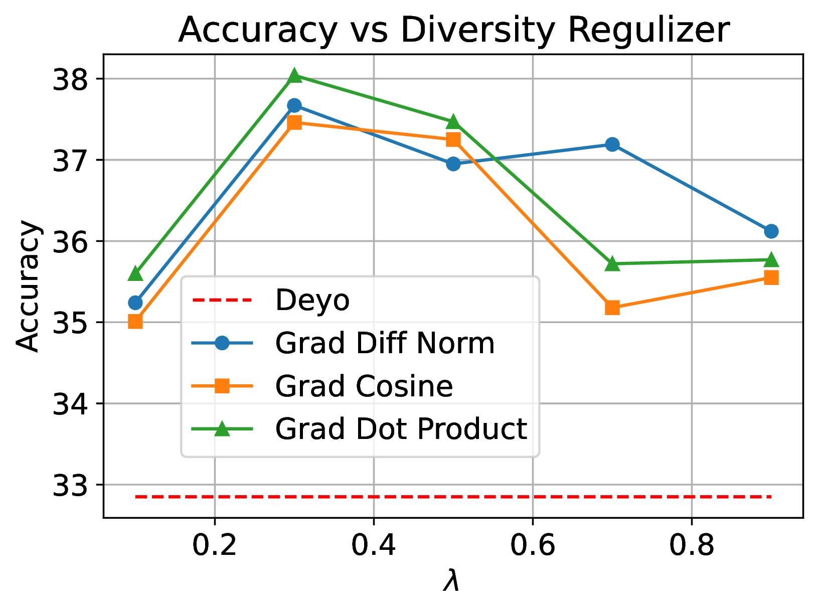
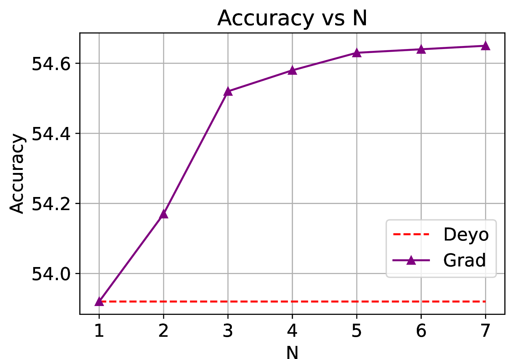
Figure 4: Ablation studies of diversification design choices on ImageNet-C under the wild test-time adaptation scenario (batch size \(1\)) using a ViTBase-LN backbone.. a — Comparison of gradient-based diversity variants on ImageNet-C with zoom blur corruption (severity 5)., b — Impact of the particle collection size \(N\) on ImageNet-C with Gaussian corruption (severity 5).
Effect of Gradient Diversity Formulation. We evaluate three formulations of gradient-based diversification: (i) pairwise dot-product alignment (Eq. 5 ), (ii) \(\ell_2\) difference between gradients, and (iii) cosine similarity. 4 (a) reports results on ImageNet-C (Zoom Blur, severity level 5) across grid-selected values of the regularization coefficient \(\lambda\). Among the three variants, the dot-product formulation achieves the highest accuracy across most values of \(\lambda\). Unlike cosine similarity, which normalizes magnitude information, and difference norms, which penalize scale rather than directional alignment, the dot-product directly discourages shared descent directions. This suggests that reducing gradient alignment, rather than merely increasing gradient magnitude disparity, is more effective for preventing trajectory collapse under entropy minimization.
Performance peaks around \(\lambda=0.3\), indicating a balanced trade-off between entropy minimization and functional repulsion. Very large \(\lambda\) values degrade accuracy, confirming that excessive repulsion can hinder adaptation.
Sensitivity to Collection Size \(N\). We analyze the effect of the number of particles on Gaussian noise corruption (severity level 5). As shown in 4 (b), accuracy improves substantially when increasing from \(N=1\) (single-model adaptation) to \(N=3\), demonstrating the benefit of multi-trajectory exploration. Beyond \(N=3\), gains become marginal relative to computational overhead. This saturation behavior indicates that a small number of interacting particles is sufficient to capture multiple plausible low-entropy modes. Accordingly, we adopt \(N=3\) in all experiments to balance robustness and efficiency.
| Noise | Blur | |||||||
| Batch Size 1 | Gauss. | Shot | Impl. | Defoc. | Glass | Motion | Zoom | Avg. |
| VitBase-LN | 9.51 | 6.72 | 8.21 | 29.01 | 23.41 | 33.87 | 27.11 | 19.69 |
| Tent | 51.15 | 51.78 | 52.50 | 52.18 | 47.68 | 56.28 | 49.06 | 51.52 |
| SAR | 50.25 | 50.65 | 51.85 | 51.61 | 48.92 | 56.71 | 50.55 | 51.51 |
| 52.61 | 53.50 | 53.46 | 54.81 | 55.42 | 61.92 | 38.37 | 52.87 | |
| Tent + | 52.23 | 52.97 | 53.45 | 54.38 | 51.40 | 58.49 | 52.54 | 53.63 |
Plug-in Evaluation on Tent. To verify that gradient diversification is not specific to our ensemble initialization, we integrate the proposed gradient repulsion term into Tent [4]. 5 shows that Tent-Grad consistently improves over vanilla Tent and achieves competitive performance with DeYO. This demonstrates that gradient-based
functional diversification acts as a general stabilization mechanism for entropy-based TTA, independent of the underlying baseline.
5 Conclusion↩︎
We revisited entropy-based test-time adaptation through the lens of underspecification and argued that conventional single-model adaptation implicitly performs point-estimate (MAP-like) inference under highly underconstrained objectives. Such point estimates are unstable under distribution shift, often leading to trajectory collapse and reliance on spurious modes. To address this limitation, we proposed a population-based diversification framework that maintains multiple interacting adaptation particles. By introducing structured diversification at the parameter, functional (gradient), optimizer, and input levels, our method transforms TTA from brittle single-trajectory optimization into controlled multi-hypothesis exploration. Extensive experiments across ImageNet-C and related benchmarks demonstrate consistent improvements under challenging settings, including batch-size-one adaptation, label distribution shifts, and mixed corruptions. Ablation studies further confirm that gradient-based functional repulsion is particularly effective in preventing trajectory alignment under entropy minimization. Overall, our results suggest that treating test-time adaptation as a multi-hypothesis inference problem is essential for reliable deployment under distribution shift. We hope this perspective motivates future work toward principled population-based adaptation strategies that improve robustness under underspecification.
Multi-Hypothesis Test-Time Adaptation to
Mitigate Underspecification
Overview of Materials in the Appendices↩︎
Related work (Appendix 6)
Underspecification in TTA (Appendix 7)
Beyond Corruption-Based Shifts (Appendix 8)
Sample Selection and Hyperparameter Configuration (Appendix 9)
Optimization Objective of SVGD (Appendix 10)
Additional experiments regarding mild scenarios (Appendix 11)
Additional experiments associated with wild scenarios for severity level of 3 (Appendix 12)
Runtime comparison of methods (Appendix 13)
Limitation (Appendix 14)
6 Related Work↩︎
6.1 Out-of-distribution Generalization↩︎
Out-of-distribution (OOD) generalization has become a critical research area, as models deployed in real-world scenarios often encounter data that are different from the training distribution. Existing research in OOD generalization primarily focuses on domain adaptation and invariant representation learning.
Domain Adaptation & Generalization Assuming the accessibility of the distribution of target data, domain adaptation is a related field to OOD generalization. It can be considered as a specific case of OOD generalization where some prior knowledge of the target distribution is available. Techniques like adversarial domain adaptation [19] attempt to align the feature distributions of the source and target domains using adversarial objectives. Domain generalization aims to learn models that perform well across a broader set of domains, including those unseen during training. Techniques in this area, such as domain-invariant feature extraction [20], optimize for representations that minimize domain-specific information, improving generalization under OOD scenarios.
Unsupervised Domain Adaptation aims to learn generalizable models using unlabeled data, while simultaneously examining the impact of pre-training on OOD generalization. Recent approaches have demonstrated promising results by leveraging large-scale unlabeled data to learn robust representation spaces [21]–[23]. However, prior methods struggle to directly address the OOD challenge, as the learned representation spaces often retain domain-specific features used to distinguish negative samples. These domain-specific features can be ineffective or even harmful to downstream tasks.
Test Time Adaptation (TTA) [4], [7], [24] is an emerging research field that involves adapting a pre-trained model from the source domain to unlabeled data in the target domain during testing, which can improve the generalization of machine learning models to new or unseen data distributions without requiring access to labeled data. Test-time batch normalization (BN) [25] is one of the earliest methods in TTA, where the statistics of the batch normalization layers are updated using the test data, thereby allowing the model to adapt to the test distribution. TENT [4] is an approach that involves entropy minimization, where the model is adapted by minimizing the prediction uncertainty on the test data. This method encourages the model to produce more confident predictions on the test set, thereby improving its robustness to distribution shifts. [8] study the failure cases of TTA methods and propose a sharpness-aware and reliable entropy minimization method SAR, which removes partial noisy samples with large gradients and encourages model weights to go to a flat minimum so that the model is robust to the remaining noisy samples. Due to the limitation of entropy [26], [7] first illustrate the limitations of relying solely on entropy as a confidence metric for TTA. Based on the observation, they further introduce a new TTA method called DeYO, which leverages a novel proposed confidence metric, PLPD.
6.2 Simplicity Bias↩︎
Simplicity bias refers to DNNs’ tendency to favor simple patterns over more complex ones in training data. This occurs because DNNs, especially those trained with gradient-based methods, often prioritize learning features or patterns that are easier to optimize, even if these features are not the most robust or generalizable for the task. As a result, simplicity bias limits DNNs’ ability to generalize to OOD data, as the simple patterns it learned may not be valid in new, unseen environments.
Research on simplicity bias has explored how it affects model generalization and performance on OOD data. [27] were among the first to highlight that DNNs tend to prioritize learning simple patterns first, particularly in early training phases. This tendency is due to the efficiency of gradient descent, which favors features that are easier to optimize. [28] demonstrated that simplicity bias could lead models to focus on spurious correlations in training data, which impairs performance on OOD data where these correlations may not hold.
More recently, researchers have investigated approaches to mitigate simplicity bias to improve OOD generalization. [29] introduced Group DRO, a robust optimization method that forces models to learn features that generalize across different data subgroups, thus reducing reliance on simple, non-robust patterns. [30] proposed techniques based on adversarial training, where models are trained against perturbed data points, encouraging them to move beyond simpler features and to learn more generalizable representations. [31] trained a collection of models and identified only one for inference, which discovered predictive patterns normally missed by a learning algorithm because of the simplicity bias.
7 Underspecification of Entropy Minimization: A Geometric Characterization↩︎
Entropy minimization is a convenient unsupervised objective for test-time adaptation, but it does not uniquely determine a robust decision function on the target distribution. In particular, the objective encourages confidence without enforcing semantic correctness. As a result, many parameter settings can achieve essentially identical (near-minimal) entropy while inducing qualitatively different decision rules and target risks. Consistent with the discussion in Sec. 3, we formalize this underspecification phenomenon by characterizing the relevant symmetries and the (potentially large) set of entropy-minimizing solutions.
7.0.0.1 Binary case.
For clarity, we first consider binary classification (the multi-class extension is discussed at the end of this subsection). Let the model output a logit \(z_\theta(x)\in\mathbb{R}\) and predictive probability \(p_\theta(x)=\sigma(z_\theta(x))\), where \(\sigma(\cdot)\) denotes the sigmoid function. The predictive entropy for an input \(x\) is \[H_\theta(x) = - p_\theta(x)\log p_\theta(x) - \bigl(1-p_\theta(x)\bigr)\log\bigl(1-p_\theta(x)\bigr),\] and the standard entropy-minimization objective over target samples \(X^t=\{x_i\}_{i=1}^n\) is \[\mathcal{L}(\theta) = \frac{1}{n}\sum_{i=1}^n H_\theta(x_i).\]
Lemma 1 (Entropy sign symmetry). For all \(z\in\mathbb{R}\), \(H(\sigma(z))=H(\sigma(-z))\).
Proof. Since \(\sigma(-z)=1-\sigma(z)\) and binary entropy satisfies \(H(p)=H(1-p)\) for all \(p\in(0,1)\), the claim follows immediately. \(\square\)
Lemma 1 implies that entropy depends only on the magnitude \(|z|\) (i.e., confidence) and is invariant to the sign of the logit (i.e., the predicted label). Consequently, entropy minimization alone cannot distinguish between two hypotheses that are equally confident but assign opposite labels on a subset of the target samples. We make this non-identifiability explicit below.
Assume the model is sufficiently expressive such that there exist two parameter settings \(\theta_1\) and \(\theta_2\) and a constant \(M>0\) satisfying \(|z_{\theta_1}(x_i)|\ge M\) and \(|z_{\theta_2}(x_i)|\ge M\) for all \(x_i\in X^t\). Suppose further that there exists a non-empty subset \(S\subset\{1,\dots,n\}\) such that \[\operatorname{sign}\!\bigl(z_{\theta_1}(x_i)\bigr) = -\operatorname{sign}\!\bigl(z_{\theta_2}(x_i)\bigr), \qquad \forall i\in S.\] Then: (i) \(\mathcal{L}(\theta_1)\approx \mathcal{L}(\theta_2)\approx 0\) for large \(M\); (ii) the induced classifiers disagree on \(S\); and (iii) unless the true labels are constant on \(S\), the corresponding target risks differ, i.e., \(R_t(\theta_1)\neq R_t(\theta_2)\).
Proof. For each \(k\in\{1,2\}\) and each \(x_i\in X^t\), the condition \(|z_{\theta_k}(x_i)|\ge M\) with large \(M\) implies \(\sigma(z_{\theta_k}(x_i))\to 0\) or \(1\), hence \(H_{\theta_k}(x_i)\to 0\). Averaging over \(i\) yields \(\mathcal{L}(\theta_k)\to 0\), so both \(\theta_1\) and \(\theta_2\) achieve (near-)minimal entropy. By Lemma 1, flipping the sign of a logit leaves the entropy unchanged, so the objective cannot prefer \(\theta_1\) over \(\theta_2\) based on \(\mathcal{L}(\cdot)\) alone. However, the decision rules \(\operatorname{sign}(z_{\theta_1}(\cdot))\) and \(\operatorname{sign}(z_{\theta_2}(\cdot))\) disagree on \(S\) by assumption, and if the ground-truth labels are not constant on \(S\), at least one of the two hypotheses must incur strictly larger classification error on that subset, implying \(R_t(\theta_1)\neq R_t(\theta_2)\). \(\square\)
7.0.0.2 Geometric interpretation and implication for test-time adaptation.
Proposition [prop:entropy95non95identifiability] formalizes a core limitation of entropy minimization: the objective only enforces high confidence on the target samples and is invariant to certain label-flipping symmetries. Therefore, multiple high-confidence solutions can attain essentially identical entropy values while inducing different decision boundaries and target risks. In overparameterized models, such ambiguity is particularly salient because parameter space often contains directions (or transformations of the classifier head) that can invert the decision rule without materially changing confidence on the observed target samples. As a result, test-time adaptation based solely on entropy minimization should be viewed as an inherently underspecified problem, motivating structured multi-hypothesis exploration or additional constraints that break these symmetries.
7.0.0.3 Multi-class note.
For \(K>2\) classes, exact global sign symmetry does not carry over, but a closely related underspecification persists: the entropy depends only on the predicted probability vector and is invariant to permutations of class identities. In particular, for any permutation \(\pi\) of \(\{1,\dots,K\}\) and any probability vector \(p\in\Delta^{K-1}\), we have \(H(p)=H(\pi(p))\). Consequently, high-confidence assignments that map target samples to different class indices can achieve the same (near-zero) entropy while corresponding to different induced labelings and risks. This observation supports the same conclusion: entropy minimization encourages confidence but does not, by itself, identify the semantically correct classifier on the target domain. This theoretical perspective directly motivates the structured multi-hypothesis diversification strategy used in our main method.
| Dataset | Tent | SAR | DeYo | Naive | SVGD | KL | Grad |
|---|---|---|---|---|---|---|---|
| ColoredMNIST | 56.30 | 57.28 | 76.88 | 79.21 | 80.36 | 80.21 | 81.33 |
| Waterbirds | 81.88 | 83.21 | 86.47 | 87.87 | 88.31 | 88.49 | 89.21 |
| ImageNet-R | 44.28 | 43.14 | 46.7 | 48.82 | 49.31 | 49.13 | 51.34 |
| Visda-2021 | 43.88 | 43.94 | 45.41 | 45.81 | 47.11 | 46.91 | 48.46 |
8 Beyond Corruption-Based Shifts↩︎
To further assess robustness beyond corruption-based benchmarks, we conduct additional experiments on datasets exhibiting different types of distribution shift, including spurious correlations and domain shifts. Specifically, we evaluate on the ColoredMNIST and Waterbirds datasets, which introduce label–attribute correlations through color and background biases, as well as ImageNet-R [13] and VisDA-2021 [14], which contain substantial style and domain variations relative to the source distribution. For ColoredMNIST, we use a ResNet-18-BN model with batch size 64, while for Waterbirds we employ a ResNet-50-BN backbone under the same batch setting. For ImageNet-R and VisDA-2021, we follow the wild scenario and use ResNet-50-GN with batch size equal to 1. The adaptation protocol and optimization hyperparameters remain consistent across all methods for fair comparison. Table 6 reports the average target-domain accuracy over five random seeds. Among the diversification strategies, gradient-based diversification (Grad) consistently achieves the best performance, indicating that maintaining diverse adaptation trajectories improves robustness across a broader range of distribution shifts.
9 Sample Selection and Hyperparameter Configuration↩︎
To ensure a fair comparison with prior baselines, we adopt the same sample-selection strategy used in previous test-time adaptation methods. In particular, we follow the confidence-based filtering mechanism employed in SAR [8] and DeYo [7], where only reliable (non-harmful) samples are used to update the model during adaptation. Specifically, a test sample \({\mathbf{x}}\) is selected for adaptation if it satisfies two conditions: (1) the predictive entropy is below a predefined threshold \(\tau_H\), and (2) the pseudo-label probability difference (PLPD) between the original input and its patch-shuffled counterpart exceeds a predefined threshold. Following DeYo [7], the PLPD score is defined as \[\text{PLPD}_{\boldsymbol{\theta}}({\mathbf{x}}, {\mathbf{x}}') = ({\mathbf{p}}_{\boldsymbol{\theta}}({\mathbf{x}}) - {\mathbf{p}}_{\boldsymbol{\theta}}({\mathbf{x}}'))_{\hat{y}},\] where \({\mathbf{x}}\) denotes the input image, \({\mathbf{x}}'\) is the patch-shuffled version of the same image, \({\mathbf{p}}_{\boldsymbol{\theta}}(\cdot)\) denotes the predicted class probability vector, and \(\hat{y}\) is the predicted pseudo-label of the model.
Formally, we update the model using samples satisfying \[H({\mathbf{p}}_{\boldsymbol{\theta}}({\mathbf{x}})) < \tau_H \quad \text{and} \quad \text{PLPD}_{\boldsymbol{\theta}}({\mathbf{x}},{\mathbf{x}}') > \tau_{\text{PLPD}},\] where \(H(\cdot)\) denotes predictive entropy. Following prior work, we set \(\tau_H = 0.4\) and \(\tau_{\text{PLPD}} = 0.3\). Using identical filtering thresholds ensures a controlled comparison under consistent sample-selection criteria during adaptation. For our diversification strategies, hyperparameters were selected via grid search. In particular, we set the KL regularization weight to \(\lambda_{\text{KL}} = 0.01\), the gradient-based diversification weight to \(\lambda_{\text{Grad}} = 0.3\), and the SVGD kernel bandwidth to \(0.01\). These values were chosen based on stability and performance considerations and were kept fixed across all experiments once selected.
10 SVGD and its Update Rules↩︎
| Noise | Blur | Weather | Digital | ||||||||||
| CIFAR-10-C | Gauss. | Shot | Impl. | Speckle | Gauss. | Brit. | Spatter | Contr. | Elastic | Pixel | JPEG | Satruate | Avg. |
| CLIP-ViT-B-32 | 25.21 | 36.70 | 31.3 | 34.21 | 51.02 | 88.40 | 67.18 | 76.98 | 31.26 | 56.30 | 28.90 | 43.21 | 47.55 |
| Tent | 13.54 | 16.01 | 12.67 | 16.04 | 71.45 | 94.79 | 80.09 | 91.95 | 26.60 | 80.23 | 18.47 | 75.85 | 49.81 |
| SAR | 41.40 | 46.64 | 43.57 | 50.89 | 71.59 | 94.10 | 79.22 | 78.75 | 68.91 | 78.79 | 52.78 | 85.62 | 66.02 |
| 33.35 | 42.20 | 20.69 | 43.87 | 67.70 | 88.14 | 76.78 | 86.45 | 55.13 | 75.73 | 40.50 | 84.30 | 59.57 | |
| 62.02 | 72.30 | 64.48 | 73.14 | 86.08 | 92.28 | 87.56 | 92.01 | 75.47 | 86.96 | 64.62 | 90.24 | 78.93 | |
| 61.28 | 72.21 | 61.76 | 72.01 | 79.63 | 92.13 | 86.01 | 89.38 | 78.73 | 85.34 | 64.78 | 90.17 | 77.79 | |
| 34.63 | 46.21 | 35.82 | 42.85 | 71.58 | 87.52 | 68.90 | 88.43 | 61.27 | 77.86 | 57.40 | 81.46 | 62.83 | |
| 62.82 | 72.47 | 60.04 | 75.60 | 85.73 | 92.49 | 87.49 | 91.82 | 78.44 | 86.74 | 65.68 | 90.07 | 79.12 | |
| Noise | Blur | Weather | Digital | ||||||||||
| CIFAR-100-C | Gauss. | Shot | Impl. | Speckle | Gauss. | Brit. | Spatter | Contr. | Elastic | Pixel | JPEG | Satruate | Avg. |
| CLIP-ViT-B-32 | 5.8 | 20.01 | 4.24 | 11.36 | 23.31 | 56.62 | 21.67 | 22.23 | 11.39 | 27.86 | 6.71 | 19.81 | 19.25 |
| Tent | 1.93 | 2.16 | 1.98 | 3.15 | 55.13 | 79.94 | 28.52 | 9.61 | 9.84 | 31.80 | 4.68 | 22.62 | 20.95 |
| SAR | 11.71 | 16.13 | 13.75 | 18.41 | 59.79 | 80.28 | 55.27 | 27.94 | 42.54 | 52.75 | 23.72 | 33.94 | 36.35 |
| 10.60 | 25.15 | 4.27 | 21.23 | 69.37 | 78.77 | 56.89 | 70.33 | 19.40 | 60.69 | 9.17 | 63.39 | 40.77 | |
| 11.28 | 31.87 | 8.26 | 31.43 | 73.56 | 79.71 | 67.50 | 74.34 | 40.75 | 68.67 | 8.78 | 64.98 | 46.76 | |
| 8.28 | 32.08 | 9.01 | 31.29 | 73.01 | 80.41 | 65.91 | 73.51 | 40.98 | 66.31 | 8.28 | 64.86 | 46.16 | |
| 9.31 | 31.41 | 7.67 | 30.49 | 72.47 | 77.91 | 66.71 | 73.13 | 40.89 | 67.73 | 8.28 | 64.01 | 45.83 | |
| 10.88 | 34.27 | 9.44 | 32.58 | 73.56 | 80.21 | 68.15 | 74.68 | 41.58 | 68.91 | 11.31 | 65.04 | 47.55 | |
| Noise | Blur | Weather | Digital | |||||||||||||
| Mild | Gauss. | Shot | Impl. | Defoc. | Glass | Motion | Zoom | Snow | Frost | Fog | Brit. | Contr. | Elastic | Pixel | JPEG | Avg. |
| ResNet-50-BN | 27.61 | 25.02 | 25.22 | 37.89 | 16.88 | 37.71 | 35.21 | 35.21 | 32.07 | 46.68 | 69.61 | 46.01 | 55.58 | 46.19 | 59.32 | 39.76 |
| Tent | 29.18 | 31.23 | 30.12 | 28.20 | 27.63 | 41.43 | 49.41 | 47.21 | 41.51 | 57.68 | 67.50 | 29.38 | 54.78 | 58.60 | 52.45 | 43.09 |
| SAR | 28.67 | 31.67 | 30.40 | 28.07 | 26.84 | 42.16 | 49.64 | 47.55 | 42.68 | 57.66 | 67.42 | 38.71 | 54.36 | 58.56 | 52.53 | 43.79 |
| 34.58 | 36.92 | 36.10 | 32.76 | 33.14 | 47.55 | 51.77 | 51.67 | 45.39 | 59.57 | 66.95 | 45.07 | 57.42 | 60.49 | 54.71 | 47.61 | |
| 35.52 | 37.34 | 37.78 | 35.02 | 33.84 | 48.11 | 52.23 | 52.28 | 45.85 | 60.35 | 67.86 | 45.53 | 57.64 | 61.29 | 54.73 | 48.36 | |
| 36.07 | 38.10 | 37.55 | 35.02 | 34.70 | 48.58 | 52.90 | 52.48 | 46.51 | 60.57 | 67.96 | 46.44 | 58.52 | 61.43 | 55.61 | 48.83 | |
| 36.15 | 38.07 | 37.46 | 34.88 | 34.28 | 48.57 | 52.91 | 52.59 | 46.40 | 60.48 | 67.97 | 45.34 | 58.52 | 61.37 | 55.73 | 48.71 | |
| 36.12 | 38.28 | 37.50 | 35.19 | 34.66 | 48.53 | 52.86 | 52.56 | 46.41 | 60.45 | 68.26 | 46.69 | 58.46 | 61.39 | 55.71 | 48.87 | |
SVGD or Stein Variational Gradient Descent [32], is a particle-based variational inference algorithm. It aims to approximate a target distribution by evolving a set of particles, which are essentially points in the parameter space. These particles are iteratively moved to better represent the target distribution using a combination of variational principles and gradient-based optimization. Mathematically, the update rule for each particle is: \[{\boldsymbol{\theta}}^{b}_i = {\boldsymbol{\theta}}^{b-1}_i + \epsilon \hat{\phi}^*({\boldsymbol{\theta}}^{b-1}_i),\] where \[\begin{align} \hat{\phi}^*({\boldsymbol{\theta}}^{b-1}_i) &= \frac{1}{N} \sum^{N}_{l=1} (k({\boldsymbol{\theta}}^{b-1}_l, {\boldsymbol{\theta}}^{b-1}_i) \nabla_{{\boldsymbol{\theta}}^{b-1}_l} \log p({\boldsymbol{\theta}}^{b-1}_l) \\ & + \nabla_{{\boldsymbol{\theta}}^{b-1}_l} k({\boldsymbol{\theta}}^{b-1}_l, {\boldsymbol{\theta}}^{b-1}_i)) \end{align}\] Here, \(k({\boldsymbol{\theta}}^{b-1}_l, {\boldsymbol{\theta}}^{b-1}_i)\) is a kernel function that defines the similarity between \({\boldsymbol{\theta}}^{b-1}_l\) and \({\boldsymbol{\theta}}^{b-1}_i\), ensuring that the models don’t collapse and spread out properly. The first term \(k({\boldsymbol{\theta}}^{b-1}_l, {\boldsymbol{\theta}}^{b-1}_i) \nabla_{{\boldsymbol{\theta}}^{b-1}_l} \log p({\boldsymbol{\theta}}^{b-1}_l)\) moves each particle in the direction of higher probability in the target distribution by following the gradient of the log-posterior. The second term \(\nabla_{{\boldsymbol{\theta}}^{b-1}_l} k({\boldsymbol{\theta}}^{b-1}_l, {\boldsymbol{\theta}}^{b-1}_i)\), at the same time, encourages diversity among the particles by pushing them away from each other.
11 Mild Scenario↩︎
Comparison on Mild Scenario. For the mild scenario, the comparison results on CIFAR-10-C, CIFAR-100-C and ImageNet-C are reported in ¿tbl:tab:cifar-c? 7 separately. Our Grad setting consistently outperforms the baseline methods across all 12 corruption types on CIFAR-10-C and CIFAR-100-C in terms of accuracy, affirming the effectiveness of our approach. Notably, the Naive setting increases model performance by large margins (+12.91% on CIFAR-10-C and +5.99% on CIFAR-100-C) without using diversity measures. Here, the backbone is OpenCLIP [33], which differs from the version of CLIP proposed by [34] that WATT [18] utilized. On ImageNet-C benchmark, our Grad method exhibits a 1.26% higher performance on average, even when compared to DeYO, which demonstrates the state-of-the-art performance in the mild scenario. It is noted that the mean of accuracies, computed over five different random seeds, has been reported in ¿tbl:tab:cifar-c? 7.
12 Wild Scenarios with Severity Level of 3↩︎
| Noise | Blur | Weather | Digital | |||||||||||||
| Batch Size 1 | Gauss. | Shot | Impl. | Defoc. | Glass | Motion | Zoom | Snow | Frost | Fog | Brit. | Contr. | Elastic | Pixel | JPEG | Avg. |
| ResNet-50-GN | 54.5 | 52.8 | 53.1 | 44.3 | 21.2 | 49.7 | 39.2 | 54.8 | 54.0 | 55.8 | 75.4 | 69.8 | 59.6 | 59.7 | 66.3 | 54.0 |
| Tent | 58.8 | 58.5 | 58.7 | 38.2 | 26.8 | 54.9 | 42.6 | 51.6 | 38.8 | 61.9 | 75.3 | 70.0 | 62.3 | 63.6 | 66.3 | 55.2 |
| SAR | 60.3 | 59.6 | 59.5 | 46.6 | 33.0 | 57.5 | 47.8 | 57.8 | 52.8 | 65.1 | 76.7 | 71.4 | 67.3 | 66.0 | 67.8 | 59.3 |
| 64.4 | 64.5 | 63.7 | 55.2 | 46 | 63.1 | 55.9 | 62.3 | 55.8 | 69.8 | 77.0 | 73.5 | 71.5 | 70.7 | 70.2 | 64.2 | |
| 65.3 | 65.7 | 63.9 | 56.2 | 45.9 | 64.0 | 56.3 | 62.5 | 56.2 | 71.1 | 77.2 | 74.2 | 71.4 | 71.2 | 71.2 | 64.8 | |
| 66.6 | 65.6 | 65.0 | 56.8 | 46.5 | 64.5 | 57.9 | 63.8 | 57.3 | 72.6 | 77.8 | 74.5 | 71.6 | 72.6 | 71.4 | 65.7 | |
| 65.1 | 66.1 | 65.2 | 57.1 | 46.2 | 64.5 | 57.2 | 64.0 | 57.7 | 72.4 | 77.6 | 75.0 | 71.7 | 71.7 | 71.4 | 65.5 | |
| 67.2 | 67.8 | 65.7 | 58.0 | 46.9 | 64.3 | 58.5 | 65.6 | 57.5 | 73.0 | 77.7 | 76.2 | 72.1 | 72.5 | 72.0 | 66.3 | |
| VitBase-LN | 51.6 | 46.9 | 50.5 | 48.7 | 37.2 | 54.7 | 41.6 | 35.1 | 33.5 | 67.8 | 69.3 | 74.8 | 65.8 | 66.0 | 63.7 | 53.8 |
| Tent | 67.1 | 66.2 | 66.3 | 66.3 | 60.9 | 69.1 | 61.4 | 65.2 | 60.4 | 75.2 | 78.1 | 78.8 | 74.9 | 75.8 | 72.4 | 69.2 |
| SAR | 68.5 | 67.8 | 68.0 | 67.8 | 63.1 | 70.7 | 63.5 | 66.9 | 62.8 | 75.8 | 77.7 | 78.4 | 74.7 | 75.7 | 72.7 | 70.3 |
| 72.3 | 72.1 | 71.9 | 71.1 | 69.4 | 74.2 | 69.3 | 72.8 | 70.1 | 78.6 | 80.7 | 84.4 | 78.6 | 79.2 | 77.2 | 74.8 | |
| 73.1 | 72.8 | 72.3 | 71.0 | 70.1 | 74.5 | 69.6 | 72.5 | 71.2 | 79.1 | 81 | 84.5 | 79.0 | 79.5 | 77.7 | 75.2 | |
| 74.5 | 74.0 | 72.4 | 71.3 | 71.1 | 75.3 | 70.1 | 73.7 | 71.8 | 79.7 | 82.0 | 84.8 | 80.1 | 79.8 | 79.1 | 76.0 | |
| 73.8 | 74.1 | 72.4 | 71.1 | 70.8 | 75.2 | 69.9 | 73.5 | 72.2 | 79.7 | 82.3 | 84.7 | 80.3 | 80.0 | 78.6 | 75.9 | |
| 74.8 | 74.8 | 73.1 | 71.2 | 71.0 | 75.1 | 71.3 | 73.4 | 73.1 | 79.7 | 82.2 | 85.0 | 81.2 | 79.8 | 78.8 | 76.3 | |
| Noise | Blur | Weather | Digital | |||||||||||||
| Label Shifts | Gauss. | Shot | Impl. | Defoc. | Glass | Motion | Zoom | Snow | Frost | Fog | Brit. | Contr. | Elastic | Pixel | JPEG | Avg. |
| ResNet-50-GN | 54.5 | 52.9 | 53.1 | 44.4 | 21.2 | 49.8 | 39.3 | 54.9 | 54.1 | 55.8 | 75.3 | 69.7 | 59.6 | 59.7 | 66.4 | 54.1 |
| Tent | 59.1 | 58.6 | 58.3 | 39.0 | 27.9 | 54.7 | 41.1 | 51.3 | 41.4 | 62.0 | 75.2 | 70.1 | 62.3 | 63.7 | 66.4 | 55.4 |
| SAR | 60.8 | 60.5 | 60.2 | 47.9 | 36.7 | 58.2 | 49.7 | 57.9 | 53.6 | 65.0 | 76.4 | 71.0 | 67.0 | 65.8 | 67.6 | 59.9 |
| 64.9 | 63.9 | 63.3 | 54.0 | 44.9 | 62.2 | 55.1 | 61.2 | 57.9 | 69.2 | 76.9 | 73.2 | 71.2 | 70.2 | 69.8 | 63.9 | |
| 65.0 | 64.0 | 64.1 | 55.1 | 44.9 | 62.3 | 55.6 | 61.4 | 58.0 | 70.2 | 77.0 | 75.0 | 73.1 | 71.3 | 70.1 | 64.5 | |
| 65.6 | 64.4 | 64.3 | 55.9 | 46.1 | 62.9 | 56.0 | 61.7 | 59.1 | 73.4 | 78.1 | 76.5 | 73.7 | 71.9 | 71.2 | 65.4 | |
| 65.6 | 65.7 | 64.6 | 55.6 | 44.9 | 63.6 | 55.2 | 62.0 | 59.1 | 75.8 | 77.7 | 76.8 | 73.6 | 72.8 | 71.4 | 65.6 | |
| 65.6 | 65.6 | 65.1 | 55.9 | 45.9 | 65.1 | 56.7 | 63.1 | 59.1 | 77.1 | 78.6 | 76.9 | 73.8 | 72.6 | 72.8 | 66.3 | |
| ViTBase-LN | 51.5 | 46.8 | 50.4 | 48.7 | 37.1 | 54.7 | 41.6 | 35.1 | 33.3 | 68.0 | 69.3 | 74.9 | 65.9 | 66.0 | 63.6 | 53.8 |
| Tent | 68.7 | 68.0 | 68.1 | 68.2 | 63.8 | 70.9 | 63.8 | 67.6 | 41.9 | 76.3 | 78.8 | 79.5 | 75.9 | 76.7 | 73.7 | 69.5 |
| SAR | 68.8 | 68.2 | 68.4 | 68.3 | 64.7 | 71.0 | 64.2 | 68.1 | 66.0 | 76.4 | 79.0 | 79.6 | 76.2 | 77.1 | 74.1 | 71.3 |
| 71.7 | 71.6 | 71.4 | 70.6 | 68.9 | 73.9 | 69.2 | 72.4 | 69.7 | 77.9 | 80.2 | 79.5 | 78.2 | 78.7 | 76.7 | 74.0 | |
| 72.3 | 72.0 | 71.5 | 72.1 | 71.7 | 74.0 | 70.2 | 74.0 | 72.0 | 78.8 | 81.1 | 80.6 | 80.1 | 79.9 | 77.0 | 75.2 | |
| 72.1 | 73.1 | 72.4 | 73.1 | 72.3 | 74.9 | 71.3 | 73.9 | 73.1 | 78.9 | 81.2 | 82.3 | 80.6 | 80.5 | 77.3 | 75.8 | |
| 73.2 | 73.1 | 72.3 | 72.9 | 71.8 | 74.7 | 71.3 | 74.1 | 72.5 | 77.9 | 81.2 | 81.5 | 80.7 | 80.5 | 77.2 | 75.7 | |
| 74.52 | 73.5 | 74.1 | 73.8 | 72.6 | 74.7 | 71.3 | 74.7 | 72.9 | 79.0 | 81.2 | 82.1 | 80.6 | 81.2 | 77.3 | 76.2 | |
| Method | #Forward | #Backward | Other computation | GPU time (50 000 images) |
|---|---|---|---|---|
| No adapt. | 50 000 | – | n/a | 79 s |
| Tent | 50 000 | 50 000 | n/a | 91 s |
| SAR | 68 608 | 31 099 | Additional model updates | 139 s |
| DeYO | 83 843 | 25 729 | Aug. filtering | 134 s |
| 83 697 | 25 469 | |||
| 83 621 | 25 339 | Aug. filtering + [eq:grad95div] | 351 s | |
| 83 573 | 25 211 |
¿tbl:tab:imagenet-sev3? presents a comparison between the baseline methods and our diversified variants on ImageNet-C at severity level 3. The reported accuracy values are averaged over five different random seeds. It is evident that all diversified methods outperform Deyo (the previous state-of-the-art) by 2–3%, showing the effectiveness of our ensembling-like diversification strategy in mitigating the effects of underspecification.
13 Runtime↩︎
8 provides a runtime comparison of TTA methods. We evaluate the computational cost of test-time adaptation techniques by benchmarking their performance on the ImageNet-C dataset. Specifically, we use the ResNet-50-BN architecture and focus on the Gaussian noise corruption at severity level 5, comprising 50,000 images. All timing experiments are conducted on a single NVIDIA ADA A6000 GPU. Among the compared methods, SAR employs a two-step optimization procedure that involves filtering out high-entropy samples before performing adaptation. DeYO, on the other hand, combines augmentation filtering with entropy-based sample exclusion to reduce computational cost while improving stability. Our framework builds upon DeYO by introducing diversification strategies at multiple levels. In particular, for the case of three particles, the total runtime remains less than three times that of DeYO. This is because not all particles undergo adaptation for every batch. Due to the induced diversity, the particles are positioned in distinct regions of the parameter space and thus respond differently to incoming data.
14 Limitation↩︎
The limitation of our proposed wrapper lies in its increased inference overhead, which scales roughly linearly with the number of particles. For example, utilizing three particles can increase runtime by nearly a factor of three compared to a single model. This added cost arises from the diversification mechanism, which drives the particles to explore distinct regions of the parameter space and generate complementary predictions. While this results in greater computational overhead, the wrapper consistently delivers improved accuracy, making it especially suitable for applications where performance takes precedence over inference speed.