Adaptive Perturbation Selection for Contrastive Audio Decoding
June 30, 2026
Abstract
Large audio-language models (LALMs) frequently hallucinate by overriding acoustic evidence with language priors. While contrastive decoding (CD) offers training-free mitigation, existing methods rely on blunt perturbations like masking or noise, leaving structured audio transformations unexplored. We explore this design space by evaluating a diverse library of targeted audio perturbations and adaptively selecting the optimal negative branch for each task and example. First, we improve upon earlier prompt engineering by showing that a simple binary yes/no constraint reduces the model’s tendency to falsely confirm absent audio features. Second, evaluating our library across temporal, spectral, frequency, and amplitude domains reveals that optimal transformations are highly task-dependent; for instance, reversing the audio array disrupts temporal coherence, raising accuracy on the temporal order task from \(74.7\%\) to \(81.4\%\). Finally, we trained a light-weight perturbation selector on model hidden states to dynamically route negative branches, yielding an additional \(+4.3\%\) gain on the existence task.
large audio-language models, audio hallucination, contrastive decoding, adaptive perturbation
1 Introduction↩︎
Large audio-language models (LALMs) [1]–[6] score well on benchmarks but routinely hallucinate [7]–[11]. These errors typically emerge during decoding when strong textual priors dominate the output space, causing the model to generate linguistically probable text that overrides the actual acoustic reality. Contrastive decoding (CD) offers a training-free remedy [12]. By amplifying the log-probability difference between an expert model (normal input branch) and a weaker, perturbed negative branch, CD penalizes tokens driven purely by language priors. However, current applications rely on a limited set of negative branches—such as total audio masking or basic additive noise [13]—leaving the broader design space of audio perturbations largely unexplored.
In this work, we perform a systematic exploration of this uncharted design space by evaluating a diverse library of targeted audio perturbations for CD. Instead of using generic noise, we design these perturbations to target specific model failure modes. Since diverse audio tasks depend on varying acoustic characteristics, the design of a negative branch must be task-specific. It is crucial to generate meaningful contrastive examples while avoiding severe acoustic distortions that could inadvertently induce further hallucinations. Matching the perturbation to the task reveals a systematic way to suppress language priors across varied audio settings. We evaluate our method across two LALMs: Qwen2-Audio-7B-Instruct [14] and Audio Flamingo 3 [15] (henceforth AF3). Testing spans four tasks: Clotho-AQA [16], along with the existence, temporal order, and object attribute variants of the Audio Hallucination dataset [7] (henceforth AH Existence, AH Order, and AH Attribute). Our contributions are:
Prompt calibration. Constraining model outputs to a single yes/no token calibrates the model’s innate affirmative bias, raising AH Existence accuracy by \(+11\)% before any CD—more than four times the prompt engineering gain of prior work on the same model.
Perturbation library. We introduce an extensive perturbation library for audio CD, comprising 105 perturbations across 38 types covering temporal, spectral, frequency, and amplitude transformations. We show that optimal perturbations are strongly task-dependent: for AF3, a reverse-audio branch achieves \(+6.7\)% on AH Order (74.7%\(\to\)81.4%) and a pitch-shift branch achieves \(+4.4\)% on AH Existence (69.5%\(\to\)73.9%).
Adaptive selector. Because the optimal perturbation depends on both the task and the individual example, we train a lightweight selector on model hidden states to route each input to its best negative branch, adding \(+4.3\)% over the best fixed branch on AH Existence with Qwen2, with \(+9.5\)% of oracle headroom remaining.
2 Related Work↩︎
Text and vision contrastive decoding. Li et al. [12] introduced CD for text generation, contrasting a large expert LM against a smaller amateur LM to suppress repetition and topic drift. VCD [17] adapts this to vision-language models, using noise-distorted visual inputs to construct the negative branch and mitigate object hallucination. While DoLa [18] contrasts representations across layers internally, AVCD [19] extends CD to the trimodal audio-visual setting. Most relevant to our work, VACoDe [20] dynamically selects the most contrastive visual augmentation per query via softmax distance; we evaluate an analogous criterion in Section 5.4.
Contrastive decoding with audio language models. Our work builds directly on the foundational Audio-Aware Decoding (AAD) framework [13], who pioneered inference-time CD for LALMs. AAD elegantly isolates persistent language priors by contrasting standard predictions against a negative branch with no-audio; pairing this token-level subtraction with an attention-directing prompt yields substantial, training-free gains across SALMONN and Qwen2-Audio on Clotho-AQA and AH Existence. Temporal Contrastive Decoding [21] extends this approach by replacing the no-audio branch with a temporally blurred view and applying an uncertainty-gated logit update, producing improvements on MMAU and AIR-Bench. Lin et al. [22] further characterized these gains via a transition matrix, showing CD reliably corrects false audio-absence claims but cannot fix highly confident incorrect beliefs. We extend this foundation to a structured library of task-oriented perturbations, with a lightweight selector that routes among them per example.
3 Method↩︎
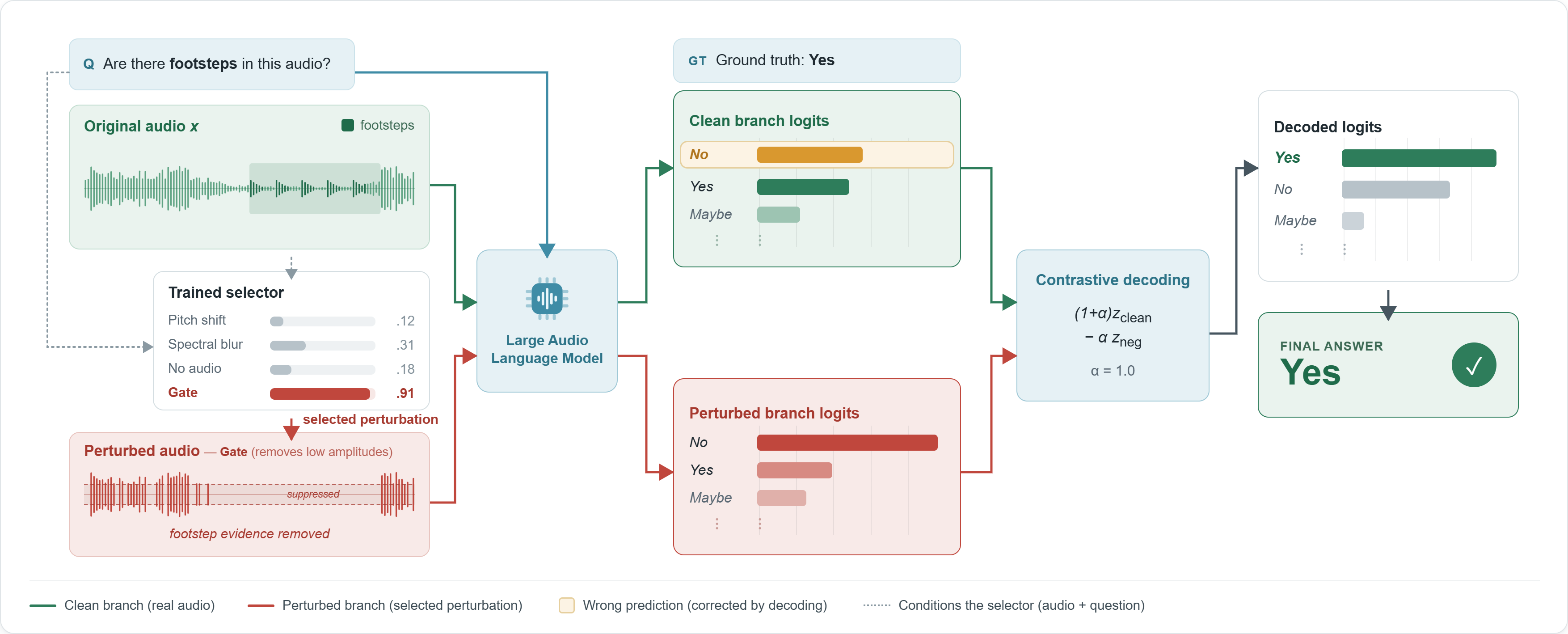
Fig. 1 illustrates our overall architecture, with each component detailed below.
3.1 Problem Setup and Contrastive Decoding↩︎
Let \(x\) be an audio clip, \(q\) a question prompt, and \(y\) an answer. The LALM produces next-token logits \[z_t = f_\theta(y_{<t},\, q,\, x),\] where \(f_\theta\) denotes the model. A perturbation \(s\) defines \(T_s(x)\). The contrastive branch logits \[z^-_{t,s} = f_\theta(y_{<t},\, q,\, T_s(x))\] are subtracted at each decoding step via a logits processor: \[\tilde{z}_{t,s} = (1 + \alpha)\,z_t - \alpha\,z^-_{t,s}, \label{eq:cd}\tag{1}\] where \(\alpha\) controls subtraction strength.
3.2 Perturbation Library↩︎
We construct a library which covers 105 perturbations across 38 types in six families. Frequency filtering uses fifth-order Butterworth filters (SciPy [23]); pitch shifting, time stretching, spectral operations, and source separation use librosa [24].
3.2.1 Temporal↩︎
Reverse: Reverses the time axis of the waveform.
Time Stretch: Phase-vocoder stretch at \(0.4\times\) and \(2.5\times\).
Segment Shuffle: Waveform divided into \(K \in \{10,50,200\}\) blocks, randomly reordered.
Segment Reverse: Each of \(K \in \{10,50\}\) blocks reversed in-place.
Dropout: Samples zero-masked at \(p \in \{0.4,0.7\}\).
Time Mask: Contiguous silence intervals up to 15% of audio duration.
Repeat Segment: A 20% slice (start or middle) looped to fill the original duration.
3.2.2 Frequency Filters↩︎
Low-Pass / High-Pass: Hard roll-offs at 250–1000 Hz and 1–6 kHz respectively.
Bandpass / Bandstop: Isolates or notches bass (50–300 Hz), mid (500–2000 Hz), or treble (3–8 kHz) bands.
Frequency Mask: Multiple random STFT bands zeroed and reconstructed via ISTFT.
3.2.3 Spectral↩︎
Pitch Shift: \(\pm4\) to \(\pm24\) semitones; duration preserved.
Spectral Noise: Gaussian noise injected into STFT magnitude (\(\sigma\) relative to magnitude RMS); phase retained.
Spectral Blur: Sequential 1D Gaussian smoothing of the STFT magnitude along time and frequency. The Gaussian standard deviation \(\sigma\), measured in STFT bins, controls the blur width and is shared across both axes (\(\sigma \in \{5,15,25\}\)).
Spectral Reverse / Segment Reverse / Segment Shuffle: Direct analogues of the temporal operations applied to STFT frame columns and reconstructed via ISTFT.
Harmonic Removal / Percussive Removal: Librosa median-filter separation on the spectrogram (margin 3.0); each retains only the tonal or transient component.
3.2.4 Amplitude & Dynamics↩︎
Hard Clip: Truncates amplitude to \(\pm\mathrm{thr}\) (\(\mathrm{thr} \in \{0.1,0.2\}\)).
Quantize: Bit depth reduced to 2–4 bits.
Compress: 10:1 or 20:1 ratio applied above threshold.
Gate / Gate Inverted: Zeros samples below or above a linear amplitude threshold.
Gate Soft / Gate Inverted Soft: Same as above with \(-12\) to \(-45\) dB attenuation instead of hard zeroing.
Normalize Chunks: Peak-normalizes \(K \in \{10,50\}\) independent temporal chunks.
Resample Low / Bit Crush: Downsample to 2–8 kHz then upsample; Bit Crush additionally reduces bit depth.
3.2.5 Environmental↩︎
Reverb / Echo: Multi-tap comb delays at 50–300 ms with configurable decay.
Phone Filter: Bandpass restricted to 300–3400 Hz.
Underwater: Low-pass at 400 Hz followed by reverb.
3.2.6 Additive Noise↩︎
- White Noise / Colored Noise: Gaussian or pink/brown noise at \(\sigma \in \{0.3\text{--}1.0\}\) relative to waveform amplitude.
3.3 Oracle Labels and Selector Training↩︎
For each example \(i\) and perturbation \(s\), let \(M_{i,s} = \mathbf{1}[\hat{y}_{i,s} = y_i]\) indicate correctness. The oracle accuracy establishes an upper bound assuming an ideal per-example selector: \[A_{\mathrm{oracle}} = \frac{1}{N}\sum_i \max_s M_{i,s}\] We train the selector (Fig. 2) using the vector \(M_i\) as a multi-label binary target, treating all correct specifications as positives. The selector itself is a lightweight neural network trained directly on the LALM’s internal hidden states to predict these targets. While the optimal choice and configuration of these hidden state representations are detailed and ablated later in Section 5.5.3, the network fundamentally learns to map the model’s internal representations to perturbation utility scores. At inference, the perturbation with the highest predicted score becomes the negative branch used for contrastive decoding.
Summary: We route each audio clip and question through the LALM twice: once with the original audio (expert branch) and once with a dynamically selected perturbed copy (negative branch). A lightweight selector, trained on the expert’s hidden states, chooses the optimal perturbation per example. The logit difference is then applied at each decoding step.

4 Experimental Setup↩︎
Datasets. Table 1 summarises the four evaluation settings. The AH benchmark [7] provides three yes/no grounding tasks. AH Existence uses 10,800 clips—created by mixing three foreground events over a background track—with multiple present/absent questions per audio combination. AH Order and AH Attribute use compositional scenes from CompA [25], testing temporal ordering and sound-attribute reasoning respectively. Lacking standard splits, we construct five balanced 70/15/15 splits per task and average results across them to reduce variance. We partition at the audio-composition level, keeping all questions from the same background-event mixture together. For AH Order and AH Attribute, this guarantees no audio files appear in both training and held-out partitions. For AH Existence, the shared clip pool makes strict audio-file separation structurally impossible; we instead minimise clip overlap between training and held-out sets. Clotho-AQA [16] provides crowd-sourced yes/no questions over FreeSound clips [26], predominantly covering existence and attribute tasks.
| Dataset | Task | Examples | Source |
|---|---|---|---|
| AH Existence | Existence Y/N | 10,800 | Synthetic composite [7] |
| AH Order | Order Y/N | 3,078 | CompA [25] |
| AH Attribute | Attribute Y/N | 1,599 | CompA [25] |
| Clotho-AQA | Mixed Y/N | 7,959 | FreeSound [26] |
Models. We evaluate on two LALMs: Qwen2-7B-Instruct [14] (Whisper-large-v2 [27] encoder, Qwen-7B backbone) and AF3 [15] (AF-Whisper encoder, Qwen2.5-7B backbone). Metrics. The primary metric is accuracy: a prediction is correct if the argmax token matches the ground-truth yes/no label. All main perturbation and selector experiments use the constrained prompt (Section 5.1).
5 Results and Analysis↩︎
5.1 Prompt Engineering and Calibration↩︎
Table ¿tbl:tab:prompts? (a) details our output prompts. Prior work [13] added an attention-directing prefix; we extend this by appending an explicit yes/no constraint—the constrained prompt used in all main experiments—significantly boosting performance.
| Prompt | Text |
|---|---|
| AAD Prompt [13] | “Focus on the given audio and answer the following question.” |
| Our Prompt | “Focus on the given audio and answer the following question with exactly one word: yes or no.” |
| No Perturbation | AAD (No-Audio) | ||||
|---|---|---|---|---|---|
| 3-4(lr)5-6 Model | Dataset | ||||
| Prompt | |||||
| Prompt | |||||
| Prompt | |||||
| Prompt | |||||
| Qwen2 | AH Existence | 56.9 | 67.9 | 70.9 | 72.4 |
| Qwen2 | AH Order | 50.4 | 51.2 | 53.2 | 52.8 |
| Qwen2 | AH Attribute | 49.9 | 51.0 | 50.7 | 51.0 |
| Qwen2 | Clotho-AQA | 72.5 | 76.1 | 78.6 | 79.6 |
| AF3 | AH Existence | 66.9 | 69.5 | 72.2 | 73.1 |
| AF3 | AH Order | 77.6 | 74.7 | 79.5 | 76.7 |
| AF3 | AH Attribute | 55.7 | 56.0 | 55.7 | 55.5 |
| AF3 | Clotho-AQA | 81.7 | 82.6 | 81.8 | 82.1 |
(a)
(b)
Under the standard AAD prompt, Qwen2 assigns “yes” to 90.4% of AH Existence examples. On this balanced dataset, this yields a \(+40.4\)% affirmative bias (predicted-yes rate minus 50%). The constrained prompt reduces this bias to \(+21.0\)%, raising accuracy from 56.9% to 67.9% (\(+11.0\)%). Applying no-audio AAD (\(\alpha=1.0\)) further shrinks residual bias to \(+1.8\)%, reaching 72.4% accuracy. The same additive pattern holds on Clotho-AQA (\(72.5\% \to 76.1\%\) from the prompt; \(76.1\% \to 79.6\%\) from no-audio contrastive decoding).
Accuracy across both models and all tasks is in Table [tbl:tab:prompt] (b). For AF3 on AH Order, the constrained prompt reduces accuracy from 77.6% to 74.7% because AF3’s bias pattern on this task differs from Qwen2’s; no-audio CD still recovers a net gain. All subsequent experiments use the constrained prompt.
5.2 Alpha Sensitivity↩︎
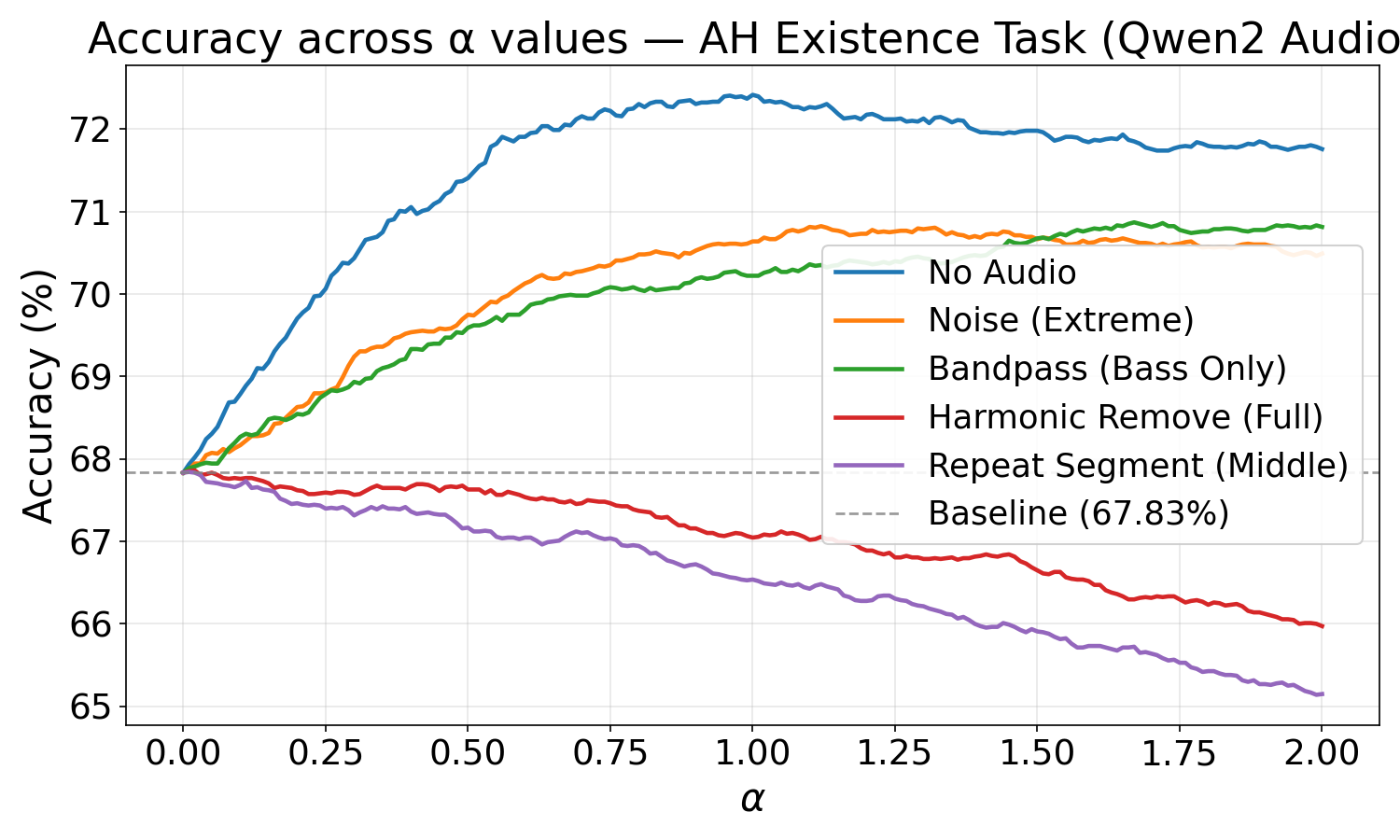
Sweeping \(\alpha \in [0, 2]\) across five representative perturbations (Fig. 3) reveals two behaviors. Helpful perturbations—no-audio, noise (\(\sigma{=}0.6\)), and bandpass (50–300 Hz)—improve with \(\alpha\), peaking near or slightly above \(\alpha=1.0\) with marginal gains before plateauing. Harmful perturbations—harmonic remove (full) and repeat segment (middle)—degrade monotonically from the outset. We avoid \(\alpha>1.0\): beyond this point the correction term outweighs the expert branch, making gains harder to interpret. We fix \(\alpha=1.0\) for remaining experiments.
5.3 Individual Perturbation Rankings↩︎
2pt
@p0.5cm@ cr | cr | cr @||@ cr | cr | cr@ & &
(lr)2-7(lr)8-13 & & & & & &
& 67.8 & & 51.2 & & 76.9 & & 69.5 & & 74.7 & & 86.7
& 86.2 & & 61.5 & & 90.1 & & 85.0 & & 90.6 & & 93.8
#1 & No-Audio & 72.4 & Reverse & 53.5 & No-Audio & 79.4 & Pitch shift & 73.9 & Reverse & 81.4 & Noise & 86.7
& & & & & &
#2 & Noise & 70.6 & Segment shuffle & 52.9 & Gate & 78.1 & Gate & 73.8 & Spectral reverse & 80.0 & Bandstop & 86.7
& & & & & &
#3 & Noise & 70.5 & No-Audio & 52.8 & Bandpass & 77.9 & Segment shuffle & 73.8 & Segment shuffle & 79.1 & Low pass & 86.7
& & & & & &
#4 & Pitch shift & 70.3 & Timestretch & 52.7 & Gate & 77.9 & Gate inv. & 73.7 & Spec.seg.shuffle & 78.9 & Gate & 86.6
& & & & & &
\(\cdots\) & & & & & &
#104 & Segment shuffle & 66.6 & Clip & 51.0 & Spectral blur & 75.7 & Spectral noise & 68.9 & Resample low & 72.7 & Dropout & 85.7
& & & & & &
#105 & Repeat segment & 66.5 & Noise & 50.8 & Spectral blur & 75.5 & Quantize & 68.6 & Normalize chunks & 71.8 & Reverb & 85.5
& & & & & &
Per-setting rankings at \(\alpha=1.0\) (Table ¿tbl:tab:perturbations?) reveal task-specific patterns.
AH Existence. For Qwen2, no-audio is the dominant branch at 72.4%, which is 4.6% above the original baseline without perturbation (67.8%). AF3 is not dominated by no-audio: pitch shift (up two octaves) leads at 73.9%, 4.4% above the original baseline (69.5%) and above no-audio at 73.1%. Conversely, Qwen2’s worst branches—segment shuffle (200 segments, 66.6%) and repeat segment (middle, 66.5%)—fall below the unmodified baseline (67.8%). Because neither removes acoustic content, the target sounds remain fully audible, providing no useful contrastive signal for existence.
AH Order. This pattern reverses for AH Order, where temporal shuffling provides a useful contrastive signal. Full waveform reversal—implemented by flipping the audio array end-to-end so the clip plays backwards—leads for both models: \(+2.4\)% for Qwen2 (51.2%\(\to\)53.5%) and \(+6.7\)% for AF3 (74.7%\(\to\)81.4%). Temporal inversion forms an ideal negative branch for order-sensitive questions.
AH Attribute. Both models score near chance (Qwen2 51.0%, AF3 56.0%) and neither respond meanginfully to constrastive decoding, with no perturbation shifting performance by more than 2%. Thus, we omit AH Attribute from Table ¿tbl:tab:perturbations?.
Clotho-AQA. AF3 is already at ceiling (86.7%) and no contrastive branch improves on the original. For Qwen2, the no-audio branch leads but gains are modest.
5.4 Distance-Based Perturbation Selection↩︎
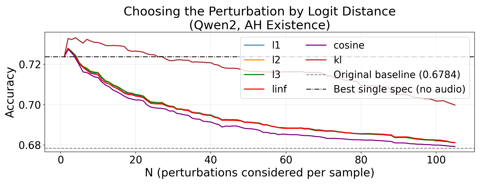
VACoDe [20] selects the negative branch that maximizes softmax divergence from the original prediction. In the visual domain, VACoDe found \(L_2\) to be the strongest metric. We evaluated the analogous strategy for audio across six distance metrics (\(L_1\), \(L_2\), \(L_3\), \(L_\infty\), cosine, KL); among our candidates, KL divergence yielded a small benefit. Applying distance-based selection across the full perturbation pool yields unstable results; we therefore report performance restricted to the top-\(N\) perturbations by aggregate accuracy (Fig. 4), the strongest variant we found. Sampling from this top-performing pool and restricting to weaker perturbations at \(\alpha=0.5\) both performed strictly worse. These outcomes suggest that logit divergence may be an unreliable proxy for contrastive utility in audio, as excessive divergence might simply trigger new hallucinations instead of cleanly isolating the intended acoustic cues.
5.5 Adaptive Selector↩︎
The adaptive selector routes each audio-question pair to one of \(N\) candidate negative branches at inference time. Trained on hidden states cached from the expert forward pass, this lightweight model requires no additional LLM computation. We evaluate four core design choices below using Qwen2 on the AH Existence task (\(\alpha=1.0\)), which provides the largest fixed-branch headroom and the clearest routing signal. Across these experiments, each variable is isolated by holding all others fixed at the optimal configuration established in the preceding ablation.
5.5.1 Number of Candidate Perturbations (\(N\))↩︎
Expanding the candidate pool continuously raises oracle performance, reaching 86.4% for Qwen2 and 85.0% for AF3 at \(N=60\) as new transformations expose distinct, solvable examples (Table ¿tbl:tab:nspec?). Conversely, selector accuracy peaks early at \(N=4\) for both models (76.7% and 76.4%) and then declines. This divergence widens the oracle-selector gap to 11.1% at \(N=60\) because larger pools dilute the training signal across the \({\approx}7{,}500\) available samples. This dilution behavior is illuminated by a greedy search over the entire 105-perturbation library: while half the library (\(N\approx51\)) guarantees maximum coverage, the performance curve effectively plateaus after \(N=10\). These steep diminishing returns confirm that the selector’s performance is strictly data-limited than candidate-limited.
r rr r@ rr r & &
(lr)2-4(lr)5-7 \(N\) & Oracle & Selector & Gap & Oracle & Selector & Gap
& 67.8 & — & — & 69.5 & — & —
1 & 72.4 & 72.4 & 0.0 & 73.9 & 73.9 & 0.0
3 & 82.9 & 76.4 & 6.5 & 80.4 & 76.1 & 4.3
4 & 83.5 & 76.7 & 6.8 & 81.3 & 76.4 & 4.9
6 & 84.4 & 76.5 & 7.9 & 82.2 & 76.4 & 5.8
10 & 85.2 & 76.1 & 9.1 & 83.2 & 76.2 & 7.0
20 & 85.9 & 75.8 &10.1 & 84.2 & 76.2 & 8.0
30 & 86.1 & 75.7 &10.4 & 84.6 & 76.0 & 8.6
60 & 86.4 & 75.3 &11.1 & 85.0 & 75.9 & 9.1
5.5.2 Head Architecture↩︎
We swept MLP depth and width; a 3-layer head with hidden dimensions [512, 256, 128] proved optimal at 76.7%, with performance degrading consistently beyond 3 layers due to overfitting.
5.5.3 Input Features↩︎
Table ¿tbl:tab:ablation? ablates input feature configurations on Qwen2 AH Existence (\(N=4\), \(\alpha=1.0\), 5 balanced splits) using 3-layer MLP selector heads.
The last token is the critical feature. While mean-pooled LLM hidden states plateau at 72.3–72.7%—effectively at the no-audio baseline (72.4%)—the last-token, last-layer state jumps to 76.3%. In a causal decoder, the final non-padding token is the only position to attend the complete input—system prompt, audio tokens, and question alike. Mean pooling dilutes this by averaging over earlier positions with partial context.
Multi-layer extraction improves further. Concatenating last-token states from first, middle, and final layers captures the representation trajectory, reaching 76.7% (\(+4.3\)% over fixed no-audio, \(+8.9\)% over the unmodified model); earlier layers contribute complementary information the final layer discards.
Separate audio features are redundant. Raw or projected audio embeddings match mean-pooled LLM states (72.5–72.6%); appending them to any LLM feature yields no reliable gain, and cross-attention (last-token \(\oplus\) audio) achieves just 76.4%—essentially matching last-token alone. External re-injection adds nothing: by the time the classifier reads the last-token state, cross-modal attention has already folded the audio signal into it during the forward pass. This generalises to AF3, where the best selector reaches 76.4% (\(N=4\)), versus the 73.1% no-audio baseline and 69.5% original.
@p5.2cm@r@
Feature configuration & Acc (%) (\(\Delta\) vs.no-audio)
Mean pool, last layer & 72.3 (\(-\)0.1)
Mean pool, all layers & 72.7 (+0.3)
Last token, last layer & 76.3 (+3.9)
Last token \(\oplus\) all-layer mean & 76.5 (+4.1)
Last token, first/mid/last layers concat. & 76.7 (+4.3)
Projected audio mean & 72.5 (+0.1)
Raw audio mean & 72.6 (+0.2)
Last token \(\oplus\) projected audio & 76.2 (+3.8)
Last token \(\oplus\) raw audio & 76.2 (+3.8)
First/mid/last \(\oplus\) projected audio & 76.6 (+4.2)
Last token \(\oplus\) audio (cross-attn) & 76.4 (+4.0)
Last-mean \(\oplus\) audio (cross-attn) & 72.4 (0.0)
5.5.4 Regularization↩︎
Overfitting is the primary bottleneck to approaching oracle performance. Because the selector is trained on a small dataset (\({\approx}\)7,500 examples) relative to a much higher-dimensional input, training and validation accuracy diverge rapidly without regularization. We explored an extensive array of strategies, including weight decay, mixup, feature dropout, input dropout, feature noise, and label smoothing. The unregularised baseline reaches 75.6% test accuracy before early stopping fires around epoch 25.
Label smoothing proves highly effective because the binary oracle targets are inherently noisy: whether branch \(A\) outperforms branch \(B\) on a finite sample reflects random variance as much as a true utility ordering. By preventing the classifier from committing to hard 0/1 targets, it allows the model to continue refining its decision boundaries without memorising label noise. Complementary strategies such as feature noise further reduce the risk of latching onto spurious feature dimensions. The optimal configuration (label smoothing \(\epsilon{=}0.25\), feature noise \(0.10\), input dropout \(0.05\)) provides a sufficient joint benefit that extends the effective training horizon to roughly 75 epochs and improves peak test accuracy to 76.7%.
5.5.5 Other Tasks↩︎
When the baseline is near chance, contrastive decoding offers little traction and the selector has no useful signal to learn from. On AH Attribute, both Qwen2 (51.0%) and AF3 (56.0%) remain near chance regardless of perturbation, consistent with prior benchmarking [7] identifying this as a fundamental capability limit. This applies to Qwen2 on AH Order, which barely exceeds chance across all branches.
AF3 on AH Order presents a different failure mode: the model is capable (74.7% baseline), yet the top perturbations are all temporal disruptions—reverse, spectral reverse, and segment shuffle—that heavily overlap in which examples they correct. Reverse dominates at 81.4%, leaving the selector little signal to improve on the fixed best branch.
On Clotho-AQA, the selector underperforms the best fixed branch as soon as more than one candidate perturbation is considered.
6 Conclusion↩︎
We demonstrate that expanding inference-time contrastive decoding beyond static baselines significantly improves a model’s ability to suppress hallucinations. While simple token constraints eliminate baseline affirmative biases, maximum performance requires task-oriented flexibility. Because the optimal negative branch varies by example, static strategies leave performance gains on the table. Our success with a lightweight selector proves a model’s internal representations already encode the necessary features to guide this adaptive selection—opening a promising new paradigm for self-correction, with substantial oracle headroom remaining.
The remaining oracle gap defines a clear research agenda:
Isolating the Routing Signal. To close the oracle gap, the selector needs datasets that actually isolate different acoustic failures. As current datasets are small, the rare cases where a complementary perturbation is uniquely useful lack the density needed for training. Building datasets that deliberately stress-test these specific situations will provide the necessary signal to improve routing.
Scaling Training Data. Progress requires not just more data but greater variety—specifically, examples where individual perturbations are each uniquely useful on distinct subsets of inputs. Datasets designed to stress-test diverse acoustic reasoning skills would provide the richer routing signal needed to close the oracle gap.
Intrinsic Perturbation Awareness. Currently, the selector relies on LALM hidden states that are unexposed to our perturbation library. Fine-tuning the LALM using contrastive objectives to explicitly predict branch utility would force its representations to natively encode these acoustic failure modes. As demonstrated by mDPO [28], models can successfully internalize corrections derived from such multimodal perturbations.
Contrastive Decoding for Open-ended Questions. While our oracle framework extends naturally to multiple-choice settings, the next major frontier is open-answer generation and captioning. Expanding adaptive CD from a single binary token to full sequence-level divergence will test the ultimate limits of perturbation-based grounding.
Acknowledgments↩︎
Parts of the experimental codebase were implemented and parts of this manuscript were drafted with assistance from Claude and Claude Code (Anthropic). The entire codebase and the paper were reviewed and edited by the authors.