Implementation Filters and Delay-Budget Instability in Coupled Replicator–Mutator Dynamics
June 30, 2026
Abstract
We model an adaptive contest in which two antagonistically coupled populations continually reallocate effort among competing methods, but decisions are not fielded instantly. Each side has an intended portfolio and a deployed portfolio: intended reallocations follow delayed observations of the opponent, while deployment follows intent through a first-order implementation filter. Under barycentric balance and uniform exploration, the linearized scalar branches have a characteristic factor in which hard observation and deployment lags enter only through their total sum, whereas implementation rates enter through real filter factors that cannot be absorbed into selection or exploration. In the strictly antagonistic class, negative spectral branches split into three regimes: weak branches have no positive-frequency crossing, intermediate branches lose stability through a delay-induced Hopf bifurcation, and strong branches are at or beyond the implementation-filter instability margin already at zero hard delay. This gives an operational delay-budget rule: in the delay-induced window, reducing any hard lag has the same first-order stabilizing leverage at onset; in the filter-induced regime, hard-lag reduction alone cannot restore stability. Balanced scalar performance observables generically show a mean shift and a second harmonic at twice the compositional frequency, and under strict antagonism the two performance signals are locked in antiphase with fixed amplitude ratio. For a baseline branch, a finite-dimensional Hopf normal-form calculation gives a negative cubic coefficient, and direct simulations reproduce the predicted threshold, amplitude scaling, and observable signatures. Motivating applications include cybersecurity and rapid technological countermeasure adaptation.
coupled replicator–mutator dynamics , implementation filters , delay differential equations , Hopf bifurcation , antagonistic coevolution , oscillations on the simplex , delay-budget instability
1 Introduction↩︎
In a fast adaptive contest, each side continually reallocates effort among competing methods, and the value of any one method depends on what the opponent currently fields. A counter that dominates today may be eroded as the other side adapts, so advantage is repeatedly won, lost, and regained rather than settled. This paper studies a minimal nonlinear mechanism by which such a contest either returns to a balanced mixed state or enters persistent oscillation.
Two features are central. The first is antagonism: a reallocation that helps one side tends, through the interaction, to reduce the value of the other side’s current mix, as in Red-Queen-type coevolution and arms-race dynamics [1], [2]. The second is implementation lag: deciding to adopt a method is not the same as fielding it at scale. The gap between decision and operative effect is familiar from implementation research [3]–[5]. In technological contests it may include validation, production, training, integration, certification, supply, and rollout. Selection may therefore be fast at the level of intention and slow at the level of deployed capability.
We model this distinction by two populations on probability simplexes. Each population has two distributions. The revision portfolio records the current intended mixture, selected from observed performance. The deployment portfolio records what has actually been fielded. Revision reacts to a delayed observation of the opponent’s deployed state, while deployment follows revision through a first-order implementation filter with a hard deployment lag and a finite implementation rate. The question is how the stability of the balanced state depends on observation delay, deployment delay, implementation speed, and antagonistic coupling.
The motivating readings are adaptive technological contests. In cybersecurity, a portfolio may consist of detection rules, patching policies, configurations, hardening measures, or offensive techniques. A rule or patch may be selected and validated before it is broadly deployed; effective coverage appears only after rollout across a population of systems. Rapid drone/counter-drone adaptation has the same mechanism-level structure: portfolios may include sensing, guidance, communications, electronic countermeasures, terminal autonomy, or interception methods. The revision layer represents intended or validated reallocations of effort; the deployment layer represents fielded kits, trained units, supply chains, and usable procedures. The model is not calibrated to a specific theatre and does not prescribe operational choices. It isolates a dynamical mechanism: stale feedback and finite fielding speed can turn local adaptation into sustained oscillation.
1.0.0.1 Relation to the author’s previous implementation-lag model
This paper continues the implementation-lag programme of [6]. That work studied a single population on a simplex under an implementation lag separating a target regime from its effective realization. Its main conclusion was that threshold restoration is preventive rather than curative: a delayed effective response may arrive after the state has already entered the basin of a competing attractor. The present paper retains the distinction between intended and effective regimes, but moves from one population to two antagonistically coupled populations, and from nonautonomous threshold passage to autonomous oscillation. The spectral object is no longer a Perron–Frobenius threshold, but the spectrum of a projected interaction product.
1.0.0.2 Prior work
The replicator equation [7], [8] and its mutation-augmented form [9] are classical. Delay-induced Hopf bifurcation in replicator dynamics is also well established. Single-population delayed replicator systems can lose stability through Hopf bifurcation under discrete, distributed, or strategy-dependent delays [10]–[15]. Delayed replicator–mutator systems have been analyzed in two-strategy symmetric games [16], and two-community replicator dynamics with discrete multi-delays has been studied without mutation [17]. We do not reclaim these Hopf mechanisms. The distinction here is structural: previous models attach delay to payoff, fitness, state information, or interaction effects, whereas the present model introduces a separate deployed state distinct from the intended state. A further structural point concerns the antagonistic core itself. In the conservative limit—no exploration, instantaneous deployment—two antagonistically coupled replicator populations are of bimatrix zero-sum type, whose interior dynamics are Hamiltonian and orbit-recurrent [8], [18]. Uniform exploration supplies damping. In the delay-induced window isolated below, the barycenter is asymptotically stable at zero hard delay. Thus the oscillation reported in that regime is not a pre-existing neutral orbit made visible by delay, but a genuine Hopf bifurcation created by delayed revision–deployment feedback. For the baseline branch used in the diagnostics, the local amplitude and frequency laws are classified in Appendix 12.
Closest to our construction are compartment and structured-population replicator models in which maturation compartments generate strategy-dependent delays and can yield Hopf bifurcations [19], [20]. In those models the compartments are life-history or population-structure stages, and the delay acts on reproduction or maturation. Here the compartments are intended and deployed portfolios of two antagonistically coupled populations, and the delay acts on strategy deployment itself. The deployment filter is also related to distributed-delay modeling and the linear chain trick [21], [22]. In that literature, gamma or Erlang kernels usually act on payoff, resource, or state variables. Here the shifted exponential kernel acts on the strategy distribution itself: a selected revision becomes deployment only after a hard lag and then accumulates with finite rate. The intended/deployed split is conceptually close to plastic/genetic two-timescale ideas in phenotypic-plasticity models [23], but the mathematical object is a coupled replicator–mutator delay system on a product of simplexes.
1.0.0.3 Contributions
We study two coupled \(m\)-strategy populations \(X,Y\), with revision portfolios \(p,q\in\Delta_m\) and deployment portfolios \(x,y\in\Delta_m\). The revision dynamics use delayed opponent deployment but current normalization, which preserves the simplexes. Deployment follows revision through shifted exponential implementation filters. The main contributions are as follows.
Two-layer simplex architecture. We formulate a revision–deployment system on \(\Delta_m^4\) and prove that the product of simplexes is forward invariant. The deployment law is an exponentially weighted memory of past revisions, shifted by a hard implementation lag. Thus a fielded portfolio can contain only what was selected earlier and then passed through the implementation pipeline.
Implementation filter factors. Under barycentric balance and uniform exploration, the linearized characteristic factor associated with a tangent spectral value \(\gamma_\rho\) has the form \[(z+\mu_X)(z+\mu_Y)(z+\kappa_X)(z+\kappa_Y) = \frac{\lambda_X\lambda_Y\kappa_X\kappa_Y}{m^2}\, \gamma_\rho e^{-z\tau_\Sigma}, \qquad \tau_\Sigma=\sigma_X+\sigma_Y+\theta_X+\theta_Y .\] The hard observation and deployment lags enter the feedback phase only through their sum \(\tau_\Sigma\). By contrast, the factors \(z+\kappa_X\) and \(z+\kappa_Y\) arise from the filter poles of the implementation layer in the loop-transfer representation. They are the fingerprint of deployment dynamics; they are not, in general, characteristic roots of the full coupled system, and they cannot be absorbed into selection or exploration rates.
Two oscillatory mechanisms. In the strictly antagonistic class \(\mathcal{B}_\rho=-\chi\mathcal{A}_\rho^\top\), the projected product has nonpositive real spectrum. A Routh–Hurwitz margin and a secant bound split negative antagonistic branches into three regimes: too weak to generate a positive-frequency crossing, genuinely delay-induced Hopf instability, and filter-induced instability already at zero hard delay. Thus oscillation may be caused by stale hard feedback, or by implementation-filter phase lag embedded in a sufficiently strong antagonistic loop.
Delay-budget triage and observable signatures. In the delay-induced window, the Hopf threshold sees the hard lags only through \(\tau_\Sigma\). Consequently all hard observation and deployment lags have the same first-order stabilizing leverage at onset. Eliminating deployment gives a finer nonlinear statement: apart from the prescribed initial histories, the reduced revision equations depend on the four hard lags through the two cross-delays \(\sigma_X+\theta_Y\) and \(\sigma_Y+\theta_X\). For compatible histories, allocations that share these cross-delays have identical reduced revision trajectories. In the filter-induced regime, however, reducing hard lags alone cannot restore stability; the relevant intervention must change the branch strength, damping, or implementation filters. The same framework gives observable diagnostics. Under barycentric balance, scalar performance observables have no linear term, so a compositional oscillation at frequency \(\omega_\ast\) produces a mean shift and a second harmonic at \(2\omega_\ast\). Under strict antagonism the two scalar performances are locked in antiphase with fixed amplitude ratio \(\chi\).
Criticality of the delay-induced onset. The general theorem gives existence and transversality. For the baseline branch we compute the cubic Hopf coefficient and obtain a negative real part, hence a supercritical locally attracting onset and the associated square-root amplitude law. We also give two branch-specific checks: an analytic sign proof for the equal-split leading branch of the diagonal \(m=3\) family and a closed-form two-strategy calculation.
In plain terms, the model says that deciding, observing, and fielding are different clocks. A contest may oscillate because agents act on stale information, or because implementation itself supplies enough phase lag under strong antagonism. In the first case, stability management is a hard-delay budget problem; in the second, hard-lag reduction is not enough. Finally, headline effectiveness can be a distorted observable: in the balanced core, an effectiveness cycle of period \(T\) corresponds to a hidden compositional race of period \(2T\).
The delayed-covariance identity recorded below is used as an interpretation, not as the proof of Hopf bifurcation. It says that selection based on delayed fitness is beneficial only while current and delayed fitness profiles remain positively aligned; if the environment changes fast enough, adaptation becomes anti-learning. The rigorous stability result follows independently from the characteristic quasipolynomial.
The paper is organized as follows. Section 2 specifies the revision–deployment model and proves simplex invariance. Section 3 records the delayed-covariance identity and its zero-delay variance limit. Section 4 derives the characteristic quasipolynomial, the zero-hard-delay stability margin, and the Hopf criterion. Section 5 analyzes asymmetry, scalar observables, and antiphase locking in the strictly antagonistic class. Section 6 gives direct numerical diagnostics of the gain window, implementation-rate dependence, time-domain behavior, a normal-form classification of the onset, amplitude scaling, and observable signatures. Section 7 discusses the mechanism, its practical reading, and its limitations.
2 Model and structural reduction↩︎
Let \[\Delta_m=\{z\in\mathbb{R}^m_{\ge0}:\mathbf{1}^\top z=1\}, \qquad u=\frac{1}{m}\mathbf{1},\] and let \[T\Delta_m=\{z\in\mathbb{R}^m:\mathbf{1}^\top z=0\}, \qquad P=I-\frac{1}{m}\mathbf{1}\mathbf{1}^\top\] be the tangent space and its orthogonal projection. Population \(X\) has a revision portfolio \(p(t)\in\Delta_m\) and a deployed portfolio \(x(t)\in\Delta_m\); population \(Y\) has \(q(t),y(t)\in\Delta_m\). The payoff matrices are \(A_\rho,B_\rho\in\mathbb{R}^{m\times m}\), with dimensionless entries. The deployed scalar performances are \[\Phi_X(x,y)=x^\top A_\rho y, \qquad \Phi_Y(y,x)=y^\top B_\rho x.\]
Revision reacts to delayed deployed opponent profiles, \[f_X^\sigma(t)=A_\rho y(t-\sigma_X), \qquad f_Y^\sigma(t)=B_\rho x(t-\sigma_Y),\] where \(\sigma_X,\sigma_Y\ge0\) are observation lags. With column-stochastic mutation matrices \(M_X,M_Y\), the revision dynamics are \[\dot{p} = \lambda_X p\odot\left[A_\rho y(t-\sigma_X)-p(t)^\top A_\rho y(t-\sigma_X)\mathbf{1}\right] +\mu_X(M_Xp-p), \label{eq:p-dynamics}\tag{1}\] \[\dot{q} = \lambda_Y q\odot\left[B_\rho x(t-\sigma_Y)-q(t)^\top B_\rho x(t-\sigma_Y)\mathbf{1}\right] +\mu_Y(M_Yq-q). \label{eq:q-dynamics}\tag{2}\] The signal is delayed but the normalization is current. This is essential: a fully delayed normalization would not, in general, preserve the affine constraint \(\mathbf{1}^\top p=1\).
Deployment follows revision through shifted exponential implementation filters, \[\dot{x}=\kappa_X[p(t-\theta_X)-x(t)], \label{eq:x-deployment}\tag{3}\] \[\dot{y}=\kappa_Y[q(t-\theta_Y)-y(t)]. \label{eq:y-deployment}\tag{4}\] Here \(\theta_X,\theta_Y\ge0\) are hard deployment lags and \(\kappa_X,\kappa_Y>0\) are implementation rates. Thus \(\sigma_i\) measures how stale the observed opponent state is, while \((\theta_i,\kappa_i)\) measures how long a selected revision takes to become fielded capability and how fast it ramps once deployment begins.
Interpretation. The model separates three clocks: observation, revision, and fielding. An agent may decide quickly but deploy slowly, or deploy quickly on outdated information. These clocks correspond to different bottlenecks in applications: sensing and intelligence on one side, production, training, integration, and rollout on the other.
Proposition 1 (simplex invariance). For continuous initial histories in \(\Delta_m^4\), the solution of 1 –4 remains in \(\Delta_m^4\) for all \(t\ge0\). If \(M_X,M_Y\) are strictly positive, the boundary of the revision simplexes is strictly repelling; in the uniform case \(M_X=M_Y=U:=u\mathbf{1}^\top\), one has \(\dot{p}_k=\mu_X/m\) at \(p_k=0\) and \(\dot{q}_k=\mu_Y/m\) at \(q_k=0\).
The proof is given in Appendix 8. The key deployment identity is \[x(t)=e^{-\kappa_X t}x(0)+\kappa_X\int_0^t e^{-\kappa_X(t-s)}p(s-\theta_X)\,ds, \label{eq:x-integral-representation}\tag{5}\] and analogously for \(y\). Away from the initial transient, this is the shifted exponential memory \[x(t)=\int_0^\infty g_X(a)p(t-a)\,da, \qquad g_X(a)=\kappa_Xe^{-\kappa_X(a-\theta_X)}\mathbf{1}_{\{a\ge\theta_X\}}. \label{eq:shifted-exponential-kernel}\tag{6}\] Thus deployment is a smeared memory of past intentions with a hard floor. A capability cannot appear in the deployed mix unless it was selected earlier and then passed through the implementation pipeline.
We analyze the interior equilibrium under a balance condition.
Assumption 1 (barycentric balance). For each admissible \(\rho\), \[A_\rho u=a_\rho\mathbf{1}, \qquad A_\rho^\top u=a_\rho\mathbf{1}, \label{eq:A-balance}\tag{7}\] \[B_\rho u=b_\rho\mathbf{1}, \qquad B_\rho^\top u=b_\rho\mathbf{1}, \label{eq:B-balance}\tag{8}\] and, whenever general mutation matrices are used, \[M_Xu=u, \qquad M_Yu=u. \label{eq:M-barycenter}\tag{9}\]
Under this assumption, \((p,q,x,y)=(u,u,u,u)\) is an equilibrium for all delays. Moreover, if \(x=u+\xi\) and \(y=u+\eta\) with \(\xi,\eta\in T\Delta_m\), then \[\Phi_X(u+\xi,u+\eta)-\Phi_X(u,u)=\xi^\top A_\rho\eta, \label{eq:PhiX-bilinear}\tag{10}\] \[\Phi_Y(u+\eta,u+\xi)-\Phi_Y(u,u)=\eta^\top B_\rho\xi. \label{eq:PhiY-bilinear}\tag{11}\] Thus the portfolio components fluctuate at first order, whereas balanced scalar performance fluctuates only at second order.
Interpretation. Near a balanced standoff, composition is a more sensitive early indicator than headline effectiveness. The mix of methods may already be cycling while aggregate performance still looks flat.
The scale/asymmetry parameter \(\rho\) is taken to deform the local interaction geometry without moving the equilibrium. A typical balance-preserving family is \[A_\rho=A_0+\rho A_1, \qquad B_\rho=B_0+\rho^{-1}B_1, \label{eq:rho-family}\tag{12}\] where each matrix satisfies the corresponding two-sided balance conditions. Define the projected matrices \[\mathcal{A}_\rho=\left.PA_\rho P\right|_{T\Delta_m}, \qquad \mathcal{B}_\rho=\left.PB_\rho P\right|_{T\Delta_m}, \label{eq:projected-matrices}\tag{13}\] and \[\mathcal{C}_\rho=\mathcal{A}_\rho\mathcal{B}_\rho. \label{eq:C-product}\tag{14}\] The strictly antagonistic class is \[\mathcal{B}_\rho=-\chi\mathcal{A}_\rho^\top, \qquad \chi>0. \label{eq:antagonistic}\tag{15}\] Then \(\mathcal{C}_\rho=-\chi\mathcal{A}_\rho\mathcal{A}_\rho^\top\) is symmetric nonpositive on \(T\Delta_m\). Negative spectral branches are therefore the local signature of antagonistic coevolution.
For local analysis, write \[p=u+\alpha, \qquad q=u+\beta, \qquad x=u+\xi, \qquad y=u+\eta, \qquad \alpha,\beta,\xi,\eta\in T\Delta_m,\] and define \[\mathcal{L}_X=\left.\mu_X(M_X-I)\right|_{T\Delta_m}, \qquad \mathcal{L}_Y=\left.\mu_Y(M_Y-I)\right|_{T\Delta_m}. \label{eq:mutation-linear-operators}\tag{16}\] The linearized tangent system is \[\dot{\alpha}=\mathcal{L}_X\alpha+\frac{\lambda_X}{m}\mathcal{A}_\rho\eta(t-\sigma_X), \qquad \dot{\beta}=\mathcal{L}_Y\beta+\frac{\lambda_Y}{m}\mathcal{B}_\rho\xi(t-\sigma_Y), \label{eq:revision-linear}\tag{17}\] \[\dot{\xi}=\kappa_X[\alpha(t-\theta_X)-\xi], \qquad \dot{\eta}=\kappa_Y[\beta(t-\theta_Y)-\eta]. \label{eq:deployment-linear}\tag{18}\] For general structured mutation, substitution of \(e^{zt}\) in 17 –18 gives the full block characteristic determinant \[\det \begin{pmatrix} zI-\mathcal{L}_X & 0 & 0 & -\dfrac{\lambda_X}{m}\mathcal{A}_\rho e^{-z\sigma_X} \\[0.5em] 0 & zI-\mathcal{L}_Y & -\dfrac{\lambda_Y}{m}\mathcal{B}_\rho e^{-z\sigma_Y} & 0 \\[0.5em] -\kappa_X e^{-z\theta_X}I & 0 & (z+\kappa_X)I & 0 \\[0.5em] 0 & -\kappa_Y e^{-z\theta_Y}I & 0 & (z+\kappa_Y)I \end{pmatrix}=0, \label{eq:general-characteristic-block}\tag{19}\] in the ordering \((\alpha,\beta,\xi,\eta)\). The deployment blocks \((z+\kappa_X)I\) and \((z+\kappa_Y)I\) are invertible away from \(z=-\kappa_X,-\kappa_Y\), and taking the Schur complement in the deployment variables \(\xi,\eta\) reduces 19 to the equivalent determinant \[\det \begin{pmatrix} zI-\mathcal{L}_X & -\dfrac{\lambda_X\kappa_Y}{m(z+\kappa_Y)}\mathcal{A}_\rho e^{-z(\sigma_X+\theta_Y)} \\[0.8em] -\dfrac{\lambda_Y\kappa_X}{m(z+\kappa_X)}\mathcal{B}_\rho e^{-z(\sigma_Y+\theta_X)} & zI-\mathcal{L}_Y \end{pmatrix}=0, \qquad z\neq-\kappa_X,-\kappa_Y. \label{eq:general-characteristic-determinant}\tag{20}\] For the analytical core we use uniform exploration, \(M_X=M_Y=U\), so that \(\mathcal{L}_X=-\mu_XI\) and \(\mathcal{L}_Y=-\mu_YI\) on \(T\Delta_m\). Then \[\det\left[D(z)I-Ke^{-z\tau_\Sigma}\mathcal{C}_\rho\right]=0, \label{eq:uniform-determinant-factor}\tag{21}\] where \[D(z)=(z+\mu_X)(z+\mu_Y)(z+\kappa_X)(z+\kappa_Y), \quad K=\frac{\lambda_X\lambda_Y\kappa_X\kappa_Y}{m^2},\] and \[\tau_\Sigma=\sigma_X+\sigma_Y+\theta_X+\theta_Y. \label{eq:total-delay}\tag{22}\] Thus each spectral value \(\gamma_\rho\in\sigma(\mathcal{C}_\rho)\) gives the scalar factor \[(z+\mu_X)(z+\mu_Y)(z+\kappa_X)(z+\kappa_Y) = \frac{\lambda_X\lambda_Y\kappa_X\kappa_Y}{m^2}\gamma_\rho e^{-z\tau_\Sigma}. \label{eq:deployment-characteristic}\tag{23}\] The determinant factorization does not require diagonalizability of \(\mathcal{C}_\rho\), although the Hopf reduction later assumes a simple critical spectral value. Since the highest-degree term is not delayed, the linearized system is retarded, not neutral. The factors \((z+\kappa_i)\) arise from the filter poles of the loop-transfer representation; they are not, in general, roots of the full characteristic equation, whose roots are shifted by the delayed coupling.
Interpretation. The corresponding filter factors \(z+\kappa_X\) and \(z+\kappa_Y\) are the mathematical fingerprint of the implementation layer. They cannot be folded into selection or exploration rates. Two agents with identical information and identical revision rules can therefore differ in stability solely because one fields faster.
The phrase “delay-induced instability” requires a zero-hard-delay stability check. Let \[r_1=\mu_X, \quad r_2=\mu_Y, \quad r_3=\kappa_X, \quad r_4=\kappa_Y,\] and define \[c_3=\sum_ir_i, \quad c_2=\sum_{i<j}r_ir_j, \quad c_1=\sum_{i<j<k}r_ir_jr_k, \quad c_\ast=\prod_ir_i.\] For a real branch \(\gamma_\rho\), set \(\Gamma_\rho=K\gamma_\rho\).
Lemma 1 (zero-delay stability for a real branch). At \(\tau_\Sigma=0\), the quartic associated with 23 is Hurwitz stable if and only if \[c_0=c_\ast-\Gamma_\rho>0 \label{eq:RH-c0}\tag{24}\] and \[(c_3c_2-c_1)c_1>c_3^2c_0. \label{eq:RH-main}\tag{25}\]
The proof is the quartic Routh–Hurwitz criterion and is recalled in Appendix 8.
Remark 2 (hard-delay-free implementation-filter instability). Let \[H=\frac{(c_3c_2-c_1)c_1}{c_3^2}.\] Then zero-delay stability is equivalent to \(c_\ast-H<\Gamma_\rho<c_\ast\). For a negative antagonistic branch, \(\Gamma_\rho=-K|\gamma_\rho|\), so zero-hard-delay stability is equivalent to \(K|\gamma_\rho|<H-c_\ast\). If this fails, the implementation filters themselves destabilize the standoff even when \(\tau_\Sigma=0\).
Interpretation. There are two oscillatory mechanisms. One is stale feedback: a race that would settle begins to oscillate because observation and deployment are too slow. The other is fielding inertia under strong antagonism: implementation filters can supply enough phase lag to destabilize the system without hard delay. These mechanisms suggest different fixes.
Finally, balanced scalar observables inherit a second harmonic.
Corollary 1 (second harmonic of balanced performance observables). Assume barycentric balance. If a critical deployed Hopf mode has \[\xi(t)=\varepsilon\operatorname{Re}(v e^{i\omega_\ast t})+\mathcal{O}(\varepsilon^2), \qquad \eta(t)=\varepsilon\operatorname{Re}(w e^{i\omega_\ast t})+\mathcal{O}(\varepsilon^2),\] then \[\Phi_X(x(t),y(t))-\Phi_X(u,u) = \frac{\varepsilon^2}{2}\operatorname{Re}(v^\top A_\rho\overline{w}) + \frac{\varepsilon^2}{2}\operatorname{Re}(v^\top A_\rho w e^{2i\omega_\ast t}) + \mathcal{O}(\varepsilon^3),\] and analogously for \(\Phi_Y\) with \(B_\rho\). Thus the leading aggregate response is a mean shift plus a second harmonic at \(2\omega_\ast\).
Interpretation. A measured effectiveness cycle of period \(T\) can correspond to an underlying compositional race of period \(2T\). Conversely, a strong first harmonic in headline effectiveness signals that the balanced core is incomplete, for instance because scale is moving at first order.
If an aggregate effective output is needed, we write \(E_i(t)=N_i(t)\Phi_i(t)\), where \(N_i\) is a slow capacity or scale variable. The analytical core treats \(N_i\) as frozen; slow capacity dynamics are discussed in the limitations and in future work, not used in the Hopf calculation.
3 Delayed covariance and lagged selection↩︎
The previous section separated revision portfolios from deployed portfolios. We now record the exact fitness identity associated with this two-layer architecture. The qualitative replacement of a variance term by a covariance term under delayed fitness information is familiar from delayed replicator models; the point here is more specific. In the coupled revision–deployment system, the identity contains an additional deployment-coupling term that has no analogue in a single-layer delayed replicator–mutator equation. The identity is used as an interpretation of lagged selection; the Hopf calculation itself proceeds through the characteristic factor 23 .
For \(r\in\Delta_m\) and \(g,h\in\mathbb{R}^m\), define \[\langle g\rangle_r=r^\top g, \qquad \operatorname{Cov}_r(g,h)=r^\top(g\odot h)-(r^\top g)(r^\top h),\] so that \(\operatorname{Var}_r(g)=\operatorname{Cov}_r(g,g)\). We evaluate the revision portfolios against the currently deployed opponent portfolios by \[\overline{F}_X(t)=p(t)^\top A_\rho y(t), \qquad \overline{F}_Y(t)=q(t)^\top B_\rho x(t).\] These quantities are not the deployed performance observables \(\Phi_X=x^\top A_\rho y\) and \(\Phi_Y=y^\top B_\rho x\); rather, they measure how the current revision portfolios would perform against the currently deployed opponent portfolios.
Proposition 3 (delayed-covariance identity). Along solutions of 1 –4 , \[\begin{align} \frac{d}{dt}\overline{F}_X(t) &=\lambda_X\operatorname{Cov}_{p(t)} \left(A_\rho y(t),A_\rho y(t-\sigma_X)\right) \\ &\quad +\mu_X(M_Xp(t)-p(t))^\top A_\rho y(t) \\ &\quad +\kappa_Yp(t)^\top A_\rho\bigl[q(t-\theta_Y)-y(t)\bigr], \end{align} \label{eq:delayed-covariance-X}\qquad{(1)}\] \[\begin{align} \frac{d}{dt}\overline{F}_Y(t) &=\lambda_Y\operatorname{Cov}_{q(t)} \left(B_\rho x(t),B_\rho x(t-\sigma_Y)\right) \\ &\quad +\mu_Y(M_Yq(t)-q(t))^\top B_\rho x(t) \\ &\quad +\kappa_Xq(t)^\top B_\rho\bigl[p(t-\theta_X)-x(t)\bigr]. \end{align} \label{eq:delayed-covariance-Y}\qquad{(2)}\]
The proof is a direct differentiation and is given in Appendix 9. The transition from an instantaneous variance to a lagged covariance is not claimed here as a new general principle; the new term in Proposition 3 is the deployment-coupling contribution.
Interpretation. A population does not simply learn from the opponent. It learns from a delayed picture of an opponent whose deployed portfolio is itself still catching up with past revisions. The covariance term measures whether that delayed picture still points in the same direction as the current fitness landscape; the deployment term measures the additional drift caused by the opponent’s implementation pipeline.
If \(\sigma_X=0\), the selection term in ?? becomes the usual variance, \[\lambda_X\operatorname{Var}_{p(t)}(A_\rho y(t)).\] For small observation delay, \[\operatorname{Cov}_{p(t)}\left(A_\rho y(t),A_\rho y(t-\sigma_X)\right) = \operatorname{Var}_{p(t)}\left(A_\rho y(t)\right) - \sigma_X\operatorname{Cov}_{p(t)}\left(A_\rho y(t),A_\rho\dot{y}(t)\right) +\mathcal{O}(\sigma_X^2). \label{eq:small-delay-covariance}\tag{26}\] Thus the first-order approximation predicts a sign reversal of the selection term when \[\sigma_X\operatorname{Cov}_{p(t)}\left(A_\rho y(t),A_\rho\dot{y}(t)\right) > \operatorname{Var}_{p(t)}\left(A_\rho y(t)\right), \label{eq:anti-learning-threshold-X}\tag{27}\] and analogously for population \(Y\), \[\sigma_Y\operatorname{Cov}_{q(t)}\left(B_\rho x(t),B_\rho\dot{x}(t)\right) > \operatorname{Var}_{q(t)}\left(B_\rho x(t)\right). \label{eq:anti-learning-threshold-Y}\tag{28}\] These are local diagnostics, not global stability criteria; the spectral Hopf threshold below gives the corresponding condition for persistent oscillatory coevolution.
Interpretation. The inequalities say when learning from delayed information turns into anti-learning. In operational language, the agent optimizes against yesterday’s opponent: the delayed signal still reports an advantage that the current environment has already erased or reversed. The Hopf threshold in the next section is the global linear version of this mechanism, describing when stale-feedback episodes reinforce rather than damp one another.
Near the barycenter, the same covariance mechanism becomes second order in the compositional perturbation. Under Assumption 1, write \[p=u+\alpha, \qquad q=u+\beta, \qquad x=u+\xi, \qquad y=u+\eta, \qquad \alpha,\beta,\xi,\eta\in T\Delta_m.\] Then the constant components of the fitness vectors cancel from the covariance, giving the following leading form.
Corollary 2 (leading covariance near the barycenter). Under Assumption 1, \[\operatorname{Cov}_{p(t)}\left(A_\rho y(t),A_\rho y(t-\sigma_X)\right) = \frac{1}{m} \left(\mathcal{A}_\rho\eta(t)\right)^\top \left(\mathcal{A}_\rho\eta(t-\sigma_X)\right) +\mathcal{O}(\|(\alpha,\eta)\|^3), \label{eq:leading-covariance-X}\tag{29}\] with the analogous identity \[\operatorname{Cov}_{q(t)}\left(B_\rho x(t),B_\rho x(t-\sigma_Y)\right) = \frac{1}{m} \left(\mathcal{B}_\rho\xi(t)\right)^\top \left(\mathcal{B}_\rho\xi(t-\sigma_Y)\right) +\mathcal{O}(\|(\beta,\xi)\|^3). \label{eq:leading-covariance-Y}\tag{30}\]
The proof, as well as the Hopf-mode expansion of 29 , is given in Appendix 9. That expansion has the same structure as Corollary 1: a balanced scalar quantity inherits a mean shift and a second harmonic rather than a leading first harmonic.
Remark 4 (balanced scalar observables inherit a second harmonic). If a scalar observable \(\Psi\) has no linear variation at the barycenter and its leading term is bilinear, \[\Psi(u+\xi,u+\eta)-\Psi(u,u)=\xi^\top H\eta+\mathcal{O}(\|(\xi,\eta)\|^3),\] then a Hopf-mode perturbation at frequency \(\omega_\ast\) produces a mean shift and a second harmonic at \(2\omega_\ast\): \[\Psi(t)-\Psi(u,u) = \frac{\varepsilon^2}{2}\operatorname{Re}(v^\top H\overline{w}) + \frac{\varepsilon^2}{2}\operatorname{Re}(v^\top H w e^{2i\omega_\ast t}) + \mathcal{O}(\varepsilon^3).\] Thus balanced scalar observables, including performance and selection-gain observables, do not generically oscillate at the Hopf frequency. A robust first harmonic in a scalar effectiveness measure indicates that the balanced core is incomplete, for example because a left-balance condition is broken or because capacity is moving at first order.
Interpretation. Scalar indicators can be misleading in two ways: they are filtered by the deployment layer, and, under balance, their leading oscillatory response is second order. Observing both the portfolio composition and the scalar output is therefore more informative than observing headline performance alone.
The next section uses the characteristic factor 23 to determine when lagged feedback destabilizes the barycentric equilibrium and produces oscillatory coevolution.
4 Linear stability and Hopf bifurcation↩︎
We now extract the stability threshold from the scalar characteristic factor 23 . Throughout this section, \[\tau=\tau_\Sigma=\sigma_X+\sigma_Y+\theta_X+\theta_Y\] denotes the total hard feedback delay, and \[r_1=\mu_X,\qquad r_2=\mu_Y,\qquad r_3=\kappa_X,\qquad r_4=\kappa_Y.\] Set \[R(z)=\prod_{j=1}^4(z+r_j) =(z+\mu_X)(z+\mu_Y)(z+\kappa_X)(z+\kappa_Y), \label{eq:R-polynomial}\tag{31}\] \[K=\frac{\lambda_X\lambda_Y\kappa_X\kappa_Y}{m^2}. \label{eq:K-coupling}\tag{32}\] For a spectral value \(\gamma\in\sigma(\mathcal{C}_\rho)\), the corresponding branch of the characteristic equation is \[F_\gamma(z,\tau):=R(z)-K\gamma e^{-z\tau}=0. \label{eq:scalar-characteristic-branch}\tag{33}\] Since the highest-degree term is not delayed, this is a retarded, not neutral, quasipolynomial. In the strictly antagonistic class 15 , \[\mathcal{C}_\rho=-\chi\mathcal{A}_\rho\mathcal{A}_\rho^\top\] is symmetric and nonpositive on \(T\Delta_m\). Thus all nonzero branches relevant for oscillation are real and negative. For such a branch, write \[L=-K\gamma=K|\gamma|>0, \label{eq:L-negative-branch}\tag{34}\] so that \[F_\gamma(z,\tau)=R(z)+L e^{-z\tau}=0. \label{eq:negative-branch-characteristic}\tag{35}\]
4.0.0.1 Imaginary roots and the delay-induced window
Let \(z=i\omega\), \(\omega>0\). Then 35 has an imaginary root only if \[R(i\omega)+L e^{-i\omega\tau}=0. \label{eq:imaginary-root-equation}\tag{36}\] Taking moduli gives \[L=|R(i\omega)|= \left[\prod_{j=1}^4(r_j^2+\omega^2)\right]^{1/2}. \label{eq:modulus-condition}\tag{37}\] The right-hand side is strictly increasing in \(\omega>0\) and equals \[c_\ast:=\prod_{j=1}^4r_j=\mu_X\mu_Y\kappa_X\kappa_Y\] at \(\omega=0\). Hence a unique positive frequency \(\omega_\ast\) exists if and only if \[L>c_\ast, \label{eq:frequency-existence-condition}\tag{38}\] and is determined by \[\prod_{j=1}^4(r_j^2+\omega_\ast^2)=L^2. \label{eq:omega-star-equation}\tag{39}\] Define \[\phi(\omega)=\arg R(i\omega)=\sum_{j=1}^4\arctan\frac{\omega}{r_j}. \label{eq:phase-function}\tag{40}\] Here \(\phi(\omega_\ast)\) is the open-loop phase of the lag cascade \(R\) at the gain-crossover frequency fixed by 39 ; the imaginary-axis condition is then the Nyquist phase-crossover condition for the delayed antagonistic feedback loop, the hard delay supplying the residual phase \(\pi-\phi(\omega_\ast)\). The corresponding critical delays are \[\tau_k(\gamma)=\frac{\pi-\phi(\omega_\ast)+2\pi k}{\omega_\ast}, \qquad \tau_k(\gamma)>0, \label{eq:critical-delays-negative}\tag{41}\] and the first such value is \[\tau_{\rm first}(\gamma)=\min\{\tau_k(\gamma)>0:k\in\mathbb{Z}\}. \label{eq:first-delay-branch}\tag{42}\] Combining 38 with the zero-delay Routh–Hurwitz margin from Lemma 1, a real negative branch lies in the genuinely delay-induced window precisely when \[c_\ast<L<H-c_\ast, \qquad H=\frac{(c_3c_2-c_1)c_1}{c_3^2}. \label{eq:delay-induced-window}\tag{43}\] The lower bound creates a positive Hopf frequency; the upper bound prevents the implementation filters from destabilizing the system already at zero hard delay.
Lemma 2 (secant bound for the implementation-filter margin). Let \(r_1,\ldots,r_4>0\), and define \[c_\ast=\prod_{j=1}^4r_j, \qquad H=\frac{(c_3c_2-c_1)c_1}{c_3^2},\] where \(c_3,c_2,c_1\) are the elementary symmetric sums of degrees one, two, and three in \(r_1,\ldots,r_4\). Then \[H-c_\ast\geq4c_\ast, \qquad\text{equivalently}\qquad H\geq5c_\ast. \label{eq:H-five-cstar}\tag{44}\] Equality holds if and only if \(r_1=r_2=r_3=r_4\). Consequently, the interval \(c_\ast<L<H-c_\ast\) is always nonempty.
Proof. See Appendix 10. ◻
Interpretation. The interval in Lemma 2 is the gain range in which a branch is strong enough to oscillate but not so strong that implementation inertia destabilizes it already at zero hard delay. Thus stronger antagonism shrinks the delay margin: as the opposition between the two adaptive responses becomes sharper, less stale feedback is needed to push the system into a persistent cycle.
4.0.0.2 Transversality
For \(\omega>0\), write \[\frac{R'(i\omega)}{R(i\omega)} =\sum_{j=1}^4\frac{1}{r_j+i\omega} =a(\omega)-i b(\omega), \label{eq:log-derivative}\tag{45}\] where \[a(\omega)=\sum_{j=1}^4\frac{r_j}{r_j^2+\omega^2}>0, \qquad b(\omega)=\sum_{j=1}^4\frac{\omega}{r_j^2+\omega^2}>0. \label{eq:a-b-definitions}\tag{46}\]
Lemma 3 (transversality for a real negative branch). Let \(\gamma<0\), and suppose that \(z=i\omega_\ast\), \(\omega_\ast>0\), is a simple root of 35 at \(\tau=\tau_k(\gamma)\). Then the root crosses the imaginary axis transversely as \(\tau\) varies. More precisely, \[\left. \frac{d}{d\tau}\operatorname{Re}z(\tau) \right|_{z=i\omega_\ast,\,\tau=\tau_k} = \frac{\omega_\ast b(\omega_\ast)}{\bigl(a(\omega_\ast)+\tau_k\bigr)^2+b(\omega_\ast)^2}>0. \label{eq:transversality-formula}\tag{47}\]
Proof. See Appendix 10. ◻
4.0.0.3 First crossing and Hopf bifurcation
Only branches satisfying \[c_\ast<L(\gamma)<H-c_\ast, \qquad L(\gamma)=K|\gamma|, \label{eq:admissible-delay-induced-branch}\tag{48}\] can contribute a genuinely delay-induced Hopf crossing. For such branches, \(\omega_\ast(\gamma)\) is determined by 39 , and \(\tau_k(\gamma)\) by 41 . The first critical hard delay in the strictly antagonistic class is \[\tau_{\rm crit} = \min_{\substack{\gamma\in\sigma(\mathcal{C}_\rho)\cap(-\infty,0)\\ c_\ast<L(\gamma)<H-c_\ast}} \;\min_{\substack{k\in\mathbb{Z}\\ \tau_k(\gamma)>0}} \tau_k(\gamma). \label{eq:global-critical-delay-antagonistic}\tag{49}\] The corresponding frequency and spectral value are denoted by \(\omega_{\rm crit}\) and \(\gamma_{\rm crit}\).
Theorem 5 (delay-induced Hopf bifurcation in the strictly antagonistic class). Assume barycentric balance and uniform exploration. Suppose that the interaction is strictly antagonistic on the tangent space, \[\mathcal{B}_\rho=-\chi\mathcal{A}_\rho^\top, \qquad \chi>0.\] Assume further that:
the barycentric equilibrium \((u,u,u,u)\) is asymptotically stable at zero hard delay; equivalently, every negative spectral branch satisfies \(L(\gamma)<H-c_\ast\);
the admissible set in 49 is nonempty, and the minimum is attained at a simple negative spectral value and a single delay branch;
no other characteristic root of the full determinant lies on the imaginary axis at \(\tau=\tau_{\rm crit}\).
Then the barycentric equilibrium is asymptotically stable for \[0\leq \tau<\tau_{\rm crit}\] and undergoes a Hopf bifurcation at \(\tau=\tau_{\rm crit}\). The critical roots are \(z=\pm i\omega_{\rm crit}\), and they cross from the left half-plane to the right half-plane as \(\tau\) increases. A local branch of periodic solutions is born at the crossing. Its criticality and stability are determined by the first Lyapunov coefficient of the retarded functional differential equation.
Proof. See Appendix 10. ◻
Interpretation. Below the critical total delay, small perturbations return to a balanced mixed state. At the crossing, the balanced standoff loses local stability and a periodic branch is born. When the postcritical branch is attracting, the dynamical reading is a back-and-forth regime: a successful revision arrives late enough to become the next source of counter-adaptation, so advantage is gained, answered, and lost rather than converging to a decisive fixed advantage. For the baseline example this branch is supercritical—the cubic Hopf coefficient computed in Appendix 12 has negative real part—but in general the threshold marks the local onset of oscillatory coevolution rather than a guarantee of global convergence to a unique cycle.
Lemma 4 (crossing recurrence and persistence of the delay-induced branch). Let \(\gamma\) be a simple negative branch with \(L=K|\gamma|\in(c_\ast,H-c_\ast)\). Then the modulus equation 37 has a unique positive root \(\omega_\ast\), and the branch meets the imaginary axis exactly at the delays \[\tau_{\rm first}(\gamma)+\frac{2\pi k}{\omega_\ast},\qquad k=0,1,2,\dots,\] every crossing being from left to right. Consequently, if no other branch crosses the imaginary axis on \([0,\tau_\Sigma]\), the barycentric equilibrium has exactly one unstable conjugate pair for \[\tau_{\rm first}(\gamma)<\tau_\Sigma<\tau_{\rm first}(\gamma)+\frac{2\pi}{\omega_\ast},\] and this instability is not removed by increasing \(\tau_\Sigma\) within that interval.
Proof. Since \(|R(i\omega)|^2=\prod_{j=1}^4(r_j^2+\omega^2)\) is strictly increasing in \(\omega>0\), the equation \(|R(i\omega)|=L\) has at most one positive root, and in the window it has exactly one, \(\omega_\ast\). An imaginary root \(z=i\omega\) of 35 forces \(|R(i\omega)|=L\), hence \(\omega=\omega_\ast\), and the balance \(Le^{-i\omega_\ast\tau}=-R(i\omega_\ast)\) gives \(\omega_\ast\tau=\pi-\phi(\omega_\ast)+2\pi k\), i.e.the displayed delays. At each of them the crossing speed is, by 47 , \(\operatorname{Re}(dz/d\tau)=\omega_\ast b(\omega_\ast)/[(a(\omega_\ast)+\tau)^2+b(\omega_\ast)^2]>0\), so every crossing is from left to right; each adds one conjugate pair to the right half-plane and none is removed, so the unstable count is constant between consecutive crossing delays. ◻
Corollary 3 (delay budget and intervention regimes). Assume barycentric balance, uniform exploration, and strict antagonism on the tangent space. Let \(\gamma<0\) be a simple spectral branch and set \(L=K|\gamma|\).
If \(L\le c_\ast\), the branch has no positive-frequency imaginary crossing and cannot set a delay-induced Hopf threshold.
If \(c_\ast<L<H-c_\ast\), the branch is asymptotically stable at zero hard delay and has a finite critical hard-delay budget \(\tau_{\rm first}(\gamma)\); for a system currently at \(\tau_\Sigma<\tau_{\rm first}(\gamma)\) the remaining margin is \(\tau_{\rm first}(\gamma)-\tau_\Sigma\). If, in addition, the branch is isolated and no other characteristic root lies on the imaginary axis at the first crossing \(\tau_{\rm first}(\gamma)\), then the crossing is transverse and, because the four hard lags enter the scalar branch only through their sum \(\tau_\Sigma\), at that crossing \[\frac{\partial\operatorname{Re}z}{\partial\sigma_X} =\frac{\partial\operatorname{Re}z}{\partial\sigma_Y} =\frac{\partial\operatorname{Re}z}{\partial\theta_X} =\frac{\partial\operatorname{Re}z}{\partial\theta_Y} =\frac{\omega_\ast\,b(\omega_\ast)}{\bigl(a(\omega_\ast)+\tau_{\rm first}(\gamma)\bigr)^2+b(\omega_\ast)^2}>0.\] Hence, to first order at the branch’s first crossing, reducing any one hard-lag component by \(\delta\) changes \(\operatorname{Re}z\) by the same amount, \(-D_\gamma\,\delta+o(\delta)\), where \(D_\gamma\) is the positive derivative displayed above, independently of which channel is shortened.
If \(L\ge H-c_\ast\), the branch is already at or beyond the implementation-filter instability margin at zero hard delay, so it is not stabilized by reducing hard observation or deployment lags alone. Stability must then be restored by lowering the branch strength \(L\) or by changing the real filter and mutation rates \(r_i\).
Proof. All three statements concern a single negative branch \(\gamma\) through its strength \(L=K|\gamma|\) and the scalar factor 35 , and none of them presupposes zero-hard-delay stability of the full system. Part (i) is the frequency-existence condition 38 : for \(L\le c_\ast\) the modulus equation 37 has no positive root. Part (iii) is Remark 2: for \(L\ge H-c_\ast\) the branch fails the zero-delay Routh–Hurwitz margin 25 , so it is already unstable at \(\tau_\Sigma=0\), and since the hard lags enter only through \(e^{-z\tau_\Sigma}\), reducing them cannot remove an instability present at zero hard delay. For part (ii), in the window \(c_\ast<L<H-c_\ast\) the branch is zero-delay stable and has a positive Hopf frequency, so the budget is finite; under the stated isolation hypothesis Lemma 3 gives a transverse crossing, and because 35 depends on \((\sigma_X,\sigma_Y,\theta_X,\theta_Y)\) only through \(\tau_\Sigma\), one has \(\partial\operatorname{Re}z/\partial\sigma_X=\cdots =\partial\operatorname{Re}z/\partial\theta_Y=d\operatorname{Re}z/d\tau\), the common value being the transversality derivative of Lemma 3 evaluated at the first crossing. ◻
Interpretation. Corollary 3 is the operational delay-budget rule, the coevolutionary counterpart of the preventive threshold of [6]. In the delay-induced window the threshold does not reveal which clock is slow: observation and deployment lags are interchangeable at first order, so the most effective action is the cheapest reduction of the total hard lag. In the filter-induced regime the diagnosis is different—shortening hard lags is not enough, and one must change the implementation filter or the effective antagonistic gain. Table 1 summarizes the resulting triage. At the baseline branch the common leverage in part (ii) is \(\approx0.080\), so each unit of total hard lag removed moves the critical root left by about \(0.08\).
| Regime | Dynamical diagnosis | Relevant intervention |
|---|---|---|
| \(L\le c_\ast\) | no delay-induced branch | monitor; locally harmless |
| \(c_\ast<L<H-c_\ast\), \(\tau_\Sigma<\tau_{\rm first}\) | stable but delay-sensitive | maintain the remaining delay margin |
| \(c_\ast<L<H-c_\ast\), \(\tau_\Sigma>\tau_{\rm first}\) | stale-feedback instability | reduce total hard lag \(\tau_\Sigma\) |
| \(L\ge H-c_\ast\) | at or beyond filter-induced margin | change filter rates or branch strength |
Remark 6 (two oscillatory mechanisms). Theorem 5 assumes zero-hard-delay stability and therefore describes a genuinely delay-induced Hopf bifurcation. If \(L\leq c_\ast\), a negative branch is too weak to generate a positive-frequency imaginary root. If \(c_\ast<L<H-c_\ast\), it is stable at zero hard delay and destabilizes only when \(\tau\) crosses \(\tau_{\rm crit}\). If \(L\geq H-c_\ast\), the implementation filters can already destabilize the system at zero hard delay. These mechanisms connect continuously: along a fixed negative branch, as \(L\uparrow H-c_\ast\) from inside the delay-induced window, \(\omega_\ast\uparrow\omega_0\), where \(\omega_0^2=c_1/c_3\) is the zero-hard-delay Hurwitz-boundary frequency, \(\phi(\omega_\ast)\uparrow\pi\), and \[\tau_0(L)=\frac{\pi-\phi(\omega_\ast(L))}{\omega_\ast(L)}\downarrow0.\] Thus the delay-induced Hopf threshold is squeezed continuously to zero as the branch approaches the filter-induced instability boundary.
Interpretation. The same observed oscillation can have different operational causes. If it is delay-induced, reducing sensing or rollout lag can restore stability. If it is filter-induced, the bottleneck is deeper: the fielding pipeline and the strength of antagonistic coupling themselves generate the phase lag.
4.0.0.4 Outside the strictly antagonistic class
For general payoff matrices, \(\mathcal{C}_\rho\) need not be symmetric and its spectrum may contain complex values. If \(\gamma=|\gamma|e^{i\psi}\) and \(L=K|\gamma|\), then the modulus condition remains \[L=|R(i\omega)|, \label{eq:complex-modulus-condition}\tag{50}\] but the phase condition becomes \[\omega\tau=\psi-\phi(\omega)+2\pi k, \qquad k\in\mathbb{Z}. \label{eq:complex-phase-condition}\tag{51}\] A complex spectral value is accompanied by its conjugate in the real linearized system. The corresponding critical block can be higher dimensional, so outside the strictly antagonistic class zero-delay stability and first crossing should be checked from the full determinant 21 or by numerical continuation.
4.0.0.5 Fast-implementation limit and critical eigenvectors
If \(\kappa_X,\kappa_Y\to\infty\) and \(\theta_X,\theta_Y\to0\), then after dividing 23 by \(\kappa_X\kappa_Y\) one obtains formally \[(z+\mu_X)(z+\mu_Y) = \frac{\lambda_X\lambda_Y}{m^2}\gamma_\rho e^{-z(\sigma_X+\sigma_Y)}. \label{eq:fast-implementation-limit-characteristic}\tag{52}\] Thus the usual two-population delayed replicator–mutator factor is recovered only as a singular fast-implementation limit.
At a critical Hopf point, write \[\alpha(t)=ae^{i\omega_\ast t},\qquad \beta(t)=be^{i\omega_\ast t},\qquad \xi(t)=re^{i\omega_\ast t},\qquad \eta(t)=se^{i\omega_\ast t}.\] The deployment layer gives \[(i\omega_\ast+\kappa_X)r=\kappa_Xa e^{-i\omega_\ast\theta_X}, \qquad (i\omega_\ast+\kappa_Y)s=\kappa_Yb e^{-i\omega_\ast\theta_Y}. \label{eq:deployment-eigenvector-relations}\tag{53}\] Hence \[\|r\|=\frac{\kappa_X}{\sqrt{\kappa_X^2+\omega_\ast^2}}\|a\|, \qquad \|s\|=\frac{\kappa_Y}{\sqrt{\kappa_Y^2+\omega_\ast^2}}\|b\|, \label{eq:deployment-amplitude-attenuation}\tag{54}\] with phase shifts \[\arg r-\arg a=-\omega_\ast\theta_X-\arctan\frac{\omega_\ast}{\kappa_X}, \qquad \arg s-\arg b=-\omega_\ast\theta_Y- \arctan\frac{\omega_\ast}{\kappa_Y}. \label{eq:deployment-phase-shifts}\tag{55}\] The hard deployment delays contribute pure phase, while finite implementation rates contribute both attenuation and additional phase lag. The next section uses these relations to separate the role of asymmetry in thresholds, amplitudes, phases, and observable second harmonics.
5 Asymmetry, modal geometry, and observable signatures↩︎
The Hopf theorem in Section 4 shows that, in the strictly antagonistic class, the onset of oscillatory coevolution is controlled by a scalar branch strength \[L(\gamma)=K|\gamma|, \qquad K=\frac{\lambda_X\lambda_Y\kappa_X\kappa_Y}{m^2},\] the pole structure \[(\mu_X,\mu_Y,\kappa_X,\kappa_Y),\] and the total hard delay \[\tau_\Sigma=\sigma_X+\sigma_Y+\theta_X+\theta_Y.\] The threshold does not distinguish how this total delay is distributed between observation and deployment. Individual lags reappear in the critical eigenvectors as phase shifts, but because the system is autonomous, absolute phases are arbitrary. The invariant information is contained in relative phases between observed harmonics and compositional modes, not in a standalone quantity such as \(\arg(r^\top A_\rho s)\). Thus the robust observable message is not a universal “difference of lags” rule. It is instead the following: balanced scalar observables inherit a mean shift and a second harmonic, while strict antagonism locks the two scalar performances in antiphase.
5.0.0.1 Branch strength and the critical delay
For a fixed negative branch in the delay-induced window \[c_\ast<L<H-c_\ast,\] the Hopf frequency \(\omega_\ast\) is determined by \[|R(i\omega_\ast)|=L, \label{eq:section5-frequency-by-L}\tag{56}\] and the principal Hopf delay is \[\tau_0(L)=\frac{\pi-\phi(\omega_\ast(L))}{\omega_\ast(L)}, \qquad \phi(\omega)=\sum_{j=1}^4\arctan\frac{\omega}{r_j}. \label{eq:principal-delay-as-function-of-L}\tag{57}\] Inside the window one has \(0<\phi(\omega_\ast)<\pi\), so \(\tau_0(L)>0\).
Proposition 7 (monotonicity of the principal Hopf delay). For fixed positive rates \(r_1,\ldots,r_4\), the principal critical delay \(\tau_0(L)\) is strictly decreasing on the delay-induced window \(c_\ast<L<H-c_\ast\). More precisely, \[\frac{d\tau_0}{dL} = -\frac{\omega_\ast a(\omega_\ast)+\pi-\phi(\omega_\ast)}{\omega_\ast^2 L b(\omega_\ast)}<0, \label{eq:dtau-dL}\qquad{(3)}\] where \[a(\omega)=\sum_{j=1}^4\frac{r_j}{r_j^2+\omega^2}, \qquad b(\omega)=\sum_{j=1}^4\frac{\omega}{r_j^2+\omega^2}.\]
Proof. See Appendix 11. ◻
Interpretation. Proposition 7 says that stronger antagonism shrinks the amount of delay needed to destabilize the branch. At the lower edge \(L\downarrow c_\ast\), the Hopf frequency tends to zero and the critical delay diverges. At the upper edge \(L\uparrow H-c_\ast\), the critical delay tends to zero, connecting continuously to the filter-induced instability of Remark 2. Stronger opposition therefore makes the adaptive contest more fragile to implementation lag.
If a balance-preserving parameter \(\rho\) deforms the projected matrices and a simple negative branch \(\gamma_\rho\) remains selected, then \[L(\rho)=K|\gamma_\rho|.\] When \(K\) is independent of \(\rho\), \[\frac{d\tau_0}{d\rho} = \frac{d\tau_0}{dL} K\frac{d|\gamma_\rho|}{d\rho}. \label{eq:dtau-drho}\tag{58}\] Thus the sign of a scale-asymmetry effect is not universal. It is determined by how the balance-preserving deformation shifts the selected spectral branch. The universal statement is only ?? : once the branch strength increases, the principal Hopf delay decreases.
5.0.0.2 What the linear threshold does not see
For a negative branch the scalar characteristic factor is \[R(z)+Le^{-z\tau_\Sigma}=0.\] Consequently, the linear Hopf threshold cannot distinguish between two decompositions of the same total hard delay. Replacing \[(\sigma_X,\sigma_Y,\theta_X,\theta_Y)\] by another quadruple with the same sum leaves the scalar threshold unchanged. The hard delays enter the eigenvector equations as unit-modulus phase factors; they do not enter the modulus condition 56 . Selection rates \(\lambda_X,\lambda_Y\) enter through their product in \(K\), whereas implementation rates \(\kappa_X,\kappa_Y\) enter both through \(K\) and through the real filter factors in \(R\). Thus implementation rates affect the threshold not merely as amplitudes, but as fielding filters.
Interpretation. A threshold calculation alone cannot tell which clock is slow. The same critical sum \(\tau_\Sigma\) may come from slow observation, slow deployment, or both. To diagnose the source of lag, one must look beyond the threshold to the modal phase geometry or to time series that resolve both composition and scalar effectiveness.
5.0.0.3 Critical eigenvectors and phase allocation
Let \(\gamma<0\) be the simple critical spectral value in the strictly antagonistic class, and let \(a\in T\Delta_m\) be a real eigenvector of \[\mathcal{C}_\rho a=\gamma a.\] At the Hopf point \(z=i\omega_\ast\), the critical eigenmode can be written as \[\alpha(t)=a e^{i\omega_\ast t}, \qquad \beta(t)=b e^{i\omega_\ast t}, \qquad \xi(t)=r e^{i\omega_\ast t}, \qquad \eta(t)=s e^{i\omega_\ast t},\] up to multiplication by a common nonzero complex scalar, which corresponds to a shift of the time origin. The deployment variables are related to the revision variables by \[r = T_X(\omega_\ast)e^{-i\omega_\ast\theta_X}a, \qquad T_X(\omega)=\frac{\kappa_X}{i\omega+\kappa_X}, \label{eq:r-from-a}\tag{59}\] \[s = T_Y(\omega_\ast)e^{-i\omega_\ast\theta_Y}b, \qquad T_Y(\omega)=\frac{\kappa_Y}{i\omega+\kappa_Y}, \label{eq:s-from-b}\tag{60}\] and \[b = S_Y(\omega_\ast)e^{-i\omega_\ast(\sigma_Y+\theta_X)}\mathcal{B}_\rho a, \qquad S_Y(\omega)= \frac{\lambda_Y\kappa_X}{m(i\omega+\mu_Y)(i\omega+\kappa_X)}. \label{eq:b-from-a}\tag{61}\] Hence \[\|r\| = \frac{\kappa_X}{\sqrt{\kappa_X^2+\omega_\ast^2}}\|a\|, \label{eq:r-amplitude}\tag{62}\] and \[\|s\| = \frac{\lambda_Y\kappa_X\kappa_Y}{m\sqrt{\mu_Y^2+\omega_\ast^2}\sqrt{\kappa_X^2+\omega_\ast^2}\sqrt{\kappa_Y^2+\omega_\ast^2}} \,\|\mathcal{B}_\rho a\|. \label{eq:s-amplitude}\tag{63}\] The associated phase shifts are \[\arg r- \arg a = -\omega_\ast\theta_X-\arctan\frac{\omega_\ast}{\kappa_X}, \label{eq:r-phase-shift}\tag{64}\] \[\arg s- \arg b = -\omega_\ast\theta_Y-\arctan\frac{\omega_\ast}{\kappa_Y}, \label{eq:s-phase-shift}\tag{65}\] and \[\arg b- \arg(\mathcal{B}_\rho a) = -\omega_\ast(\sigma_Y+\theta_X) -\arctan\frac{\omega_\ast}{\mu_Y} -\arctan\frac{\omega_\ast}{\kappa_X}. \label{eq:b-phase-shift}\tag{66}\] The individual delays therefore enter the geometry of the oscillation, not the threshold itself. They shape which deployed portfolio lags its revision signal, how strongly finite implementation attenuates it, and how scalar harmonics are phased relative to a chosen compositional reference. They do not define a normalization-independent invariant such as a universal difference of lags.
5.0.0.4 Balanced scalar observables
Under barycentric balance, aggregate deployed performance has no linear variation at the barycenter. In the notation above, Corollary 1 gives \[\Phi_X(x(t),y(t))-\Phi_X(u,u) = \frac{\varepsilon^2}{2}\operatorname{Re}(r^\top A_\rho\overline{s}) + \frac{\varepsilon^2}{2}\operatorname{Re}(r^\top A_\rho s\,e^{2i\omega_\ast t}) + \mathcal{O}(\varepsilon^3), \label{eq:section5-PhiX-second-harmonic}\tag{67}\] with the analogous expression \[\Phi_Y(y(t),x(t))-\Phi_Y(u,u) = \frac{\varepsilon^2}{2}\operatorname{Re}(s^\top B_\rho\overline{r}) + \frac{\varepsilon^2}{2}\operatorname{Re}(s^\top B_\rho r\,e^{2i\omega_\ast t}) + \mathcal{O}(\varepsilon^3). \label{eq:section5-PhiY-second-harmonic}\tag{68}\] Thus the compositional portfolios oscillate at frequency \(\omega_\ast\), whereas balanced scalar performance observables display a mean shift and a second harmonic at \(2\omega_\ast\). The phase of the second harmonic becomes meaningful only relative to a compositional reference phase or by comparison with another scalar observable.
Corollary 4 (antiphase locking of balanced scalar performances). Assume barycentric balance and strict antagonism on the tangent space, \[\mathcal{B}_\rho=-\chi\mathcal{A}_\rho^\top, \qquad \chi>0.\] For any deployed perturbations \[x=u+\xi, \qquad y=u+\eta, \qquad \xi,\eta\in T\Delta_m,\] one has \[\Phi_Y(u+\eta,u+\xi)-\Phi_Y(u,u) = -\chi\bigl[\Phi_X(u+\xi,u+\eta)-\Phi_X(u,u)\bigr]. \label{eq:antiphase-locking-exact}\tag{69}\] Consequently, the mean shifts and second harmonics of \(\Phi_X\) and \(\Phi_Y\) have amplitude ratio \(\chi\) and are in phase opposition, independently of the individual observation and deployment lags.
Proof. By 10 –11 , \[\Phi_X(u+\xi,u+\eta)-\Phi_X(u,u)=\xi^\top\mathcal{A}_\rho\eta, \qquad \Phi_Y(u+\eta,u+\xi)-\Phi_Y(u,u)=\eta^\top\mathcal{B}_\rho\xi.\] Strict antagonism gives \[\eta^\top\mathcal{B}_\rho\xi =-\chi\eta^\top\mathcal{A}_\rho^\top\xi =-\chi\xi^\top\mathcal{A}_\rho\eta,\] which proves 69 . ◻
Interpretation. An observer who sees only aggregate effectiveness may misread the tempo of the underlying adaptive race. In the balanced antagonistic core, headline effectiveness carries a second-harmonic signature, while the hidden portfolios cycle at the fundamental Hopf frequency. Strict antagonism also gives a clean cross-population signature: the two scalar effectiveness signals move in opposite phase with fixed amplitude ratio \(\chi\). This is a falsifiable signature of the model class, not merely a qualitative statement that the system oscillates.
A first harmonic can reappear in an aggregate effectiveness observable in two natural ways. First, the left-balance conditions in Assumption 1 may fail, restoring a linear term in \(\Phi_X\) or \(\Phi_Y\). Second, a scalar capacity variable can respond at first order. If \[E_X(t)=N_X(t)\Phi_X(x(t),y(t)), \qquad N_X(t)=N_X^\ast+\varepsilon n_X(t)+\mathcal{O}(\varepsilon^2),\] then \[E_X(t)-E_X^\ast = \varepsilon n_X(t)\Phi_X(u,u) + N_X^\ast\bigl[\Phi_X(x(t),y(t))-\Phi_X(u,u)\bigr] + \mathcal{O}(\varepsilon^3).\] Thus a robust first harmonic in headline effectiveness points either to broken left balance or to an additional first-order capacity channel.
The next section illustrates these analytical conclusions numerically, locating the three branch-strength regimes, the implementation-rate window, and the predicted observable signatures.
6 Numerical illustrations and operational diagnostics↩︎
The calculations in this section connect the closed-form Hopf threshold of Section 4 to reproducible time-domain behavior and to the observable signatures of Section 5. For the baseline branch we also compute the cubic Hopf coefficient from the finite normal form (Diagnostic 3 and Appendix 12); this classifies the local onset as supercritical. The simulations below illustrate the threshold, postcritical saturation, amplitude scaling, and observable signatures. They are not used as a global continuation proof for the nonlinear periodic branch.
We use one small strictly antagonistic example to address three questions that arise in applications: \[\begin{gather} \text{How strong is the antagonistic branch?}\\ \text{How fast is fielding?}\\ \text{What would an observer see?} \end{gather}\] The examples are dimensionless mechanism checks. They should not be read as a calibration to any particular empirical contest.
6.0.0.1 Baseline strictly antagonistic example
Take \(m=3\), so \(T\Delta_3\) is two-dimensional. Let \[q_1=\frac{1}{\sqrt2}(1,-1,0)^\top, \qquad q_2=\frac{1}{\sqrt6}(1,1,-2)^\top, \qquad Q=(q_1,q_2),\] and define \[A=Q \begin{pmatrix} 1&0\\0&1/2 \end{pmatrix} Q^\top = \frac{1}{12} \begin{pmatrix} 7&-5&-2\\ -5&7&-2\\ -2&-2&4 \end{pmatrix}, \qquad B=-A^\top=-A. \label{eq:num-baseline-A}\tag{70}\] Then \[Au=A^\top u=Bu=B^\top u=0,\] so barycentric balance holds with \(a_\rho=b_\rho=0\), and strict antagonism holds with \(\chi=1\). On the tangent space, \[\mathcal{C}=\mathcal{A}\mathcal{B}=-\mathcal{A}\mathcal{A}^\top,\] with eigenvalues \[\gamma_1=-1, \qquad \gamma_2=-\frac{1}{4}. \label{eq:num-gamma-values}\tag{71}\] For the baseline rates \[\mu_X=\mu_Y=1, \qquad \kappa_X=\kappa_Y=1, \qquad \lambda_X=\lambda_Y=\frac{9}{2}, \label{eq:num-baseline-rates}\tag{72}\] we have \[K=\frac{\lambda_X\lambda_Y\kappa_X\kappa_Y}{m^2}=\frac{9}{4}.\] Thus the two branch strengths are \[L_1=K|\gamma_1|=\frac{9}{4}, \qquad L_2=K|\gamma_2|=\frac{9}{16}.\] Since \(r_1=\cdots=r_4=1\), \[c_\ast=1, \qquad H=5, \qquad c_\ast<L<H-c_\ast \quad\Longleftrightarrow\quad 1<L<4.\] Only the first branch is in the delay-induced Hopf window; the second branch is too weak to generate a positive-frequency crossing. For the critical branch, \[|R(i\omega)|=(1+\omega^2)^2=L_1=\frac{9}{4},\] so \[\omega_\ast=\frac{1}{\sqrt2},\] and \[\tau_{\rm crit} = \frac{\pi-4\arctan(1/\sqrt2)}{1/\sqrt2} \approx0.9612. \label{eq:num-baseline-taucrit}\tag{73}\] The linear Hopf prediction gives the compositional period \[T_{\rm comp}=\frac{2\pi}{\omega_\ast}\approx8.886,\] whereas a balanced scalar observable has leading period \[T_{\rm scalar}=\frac{\pi}{\omega_\ast}\approx4.443.\]
Interpretation. The example selects one dangerous mode and one harmless mode from the same local interaction geometry. The stronger branch is not unstable by itself; it becomes unstable only when the total feedback delay exceeds about \(0.96\). The weaker branch does not generate a positive-frequency linear Hopf crossing at any hard delay.
6.0.0.2 Diagnostic 1: branch strength and the delay margin
For the equal-pole case \(r_1=\cdots=r_4=1\), the principal critical delay is an explicit function of branch strength: \[\omega(L)=\sqrt{\sqrt L-1}, \qquad \tau_0(L)=\frac{\pi-4\arctan \omega(L)}{\omega(L)}, \qquad 1<L<4.\] Figure 1 displays this curve and marks the baseline branch \(L=9/4\).
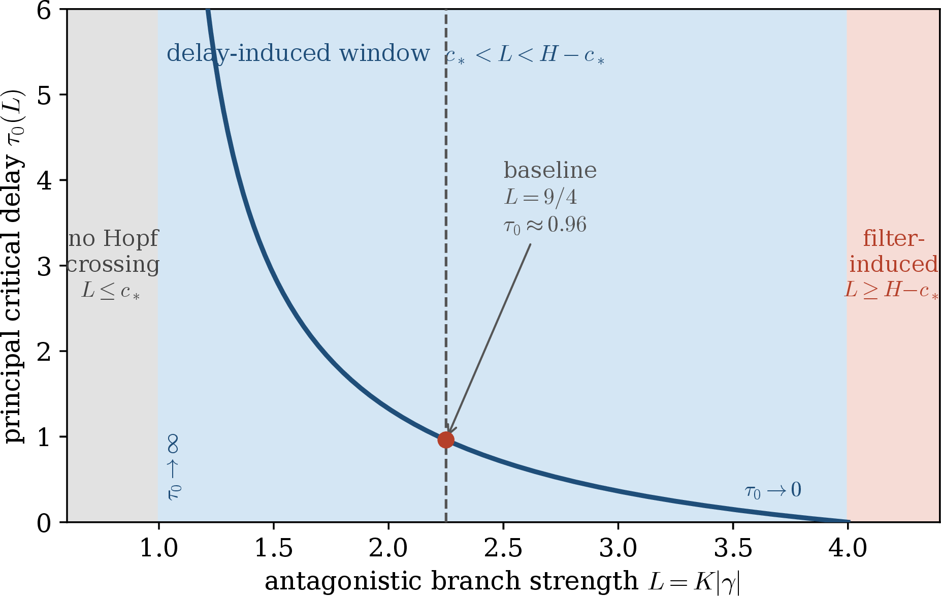
Interpretation. The plot separates three operational regimes. Weak branches are locally harmless in the linear Hopf sense: \(L\leq c_\ast\) gives no positive-frequency crossing. Intermediate branches are delay-sensitive: \(c_\ast<L<H-c_\ast\) gives a finite delay margin. Very strong branches are filter-unstable: \(L\geq H-c_\ast\) can destabilize the system even at zero hard delay. Thus reducing delay is the right intervention only in the middle regime; outside it, the branch is either too weak to matter or too strong for the implementation filters to stabilize.
6.0.0.3 Diagnostic 2: implementation speed as a fielding lever
We next vary the implementation speed while holding the branch strength fixed. Set \[\mu_X=\mu_Y=1, \qquad \kappa_X=\kappa_Y=\kappa, \qquad L=\frac{9}{4}.\] Then \[|R(i\omega)|=(1+\omega^2)(\kappa^2+\omega^2),\] and the principal delay is computed from \[(1+\omega_\ast^2)(\kappa^2+\omega_\ast^2)=\frac{9}{4},\] \[\tau_0(\kappa)= \frac{\pi-2\arctan(\omega_\ast)-2\arctan(\omega_\ast/\kappa)}{\omega_\ast}.\] The delay-induced window exists only when \[c_\ast(\kappa)<\frac{9}{4}<H(\kappa)-c_\ast(\kappa).\] For this example, this gives approximately \[0.7417<\kappa<1.5.\]
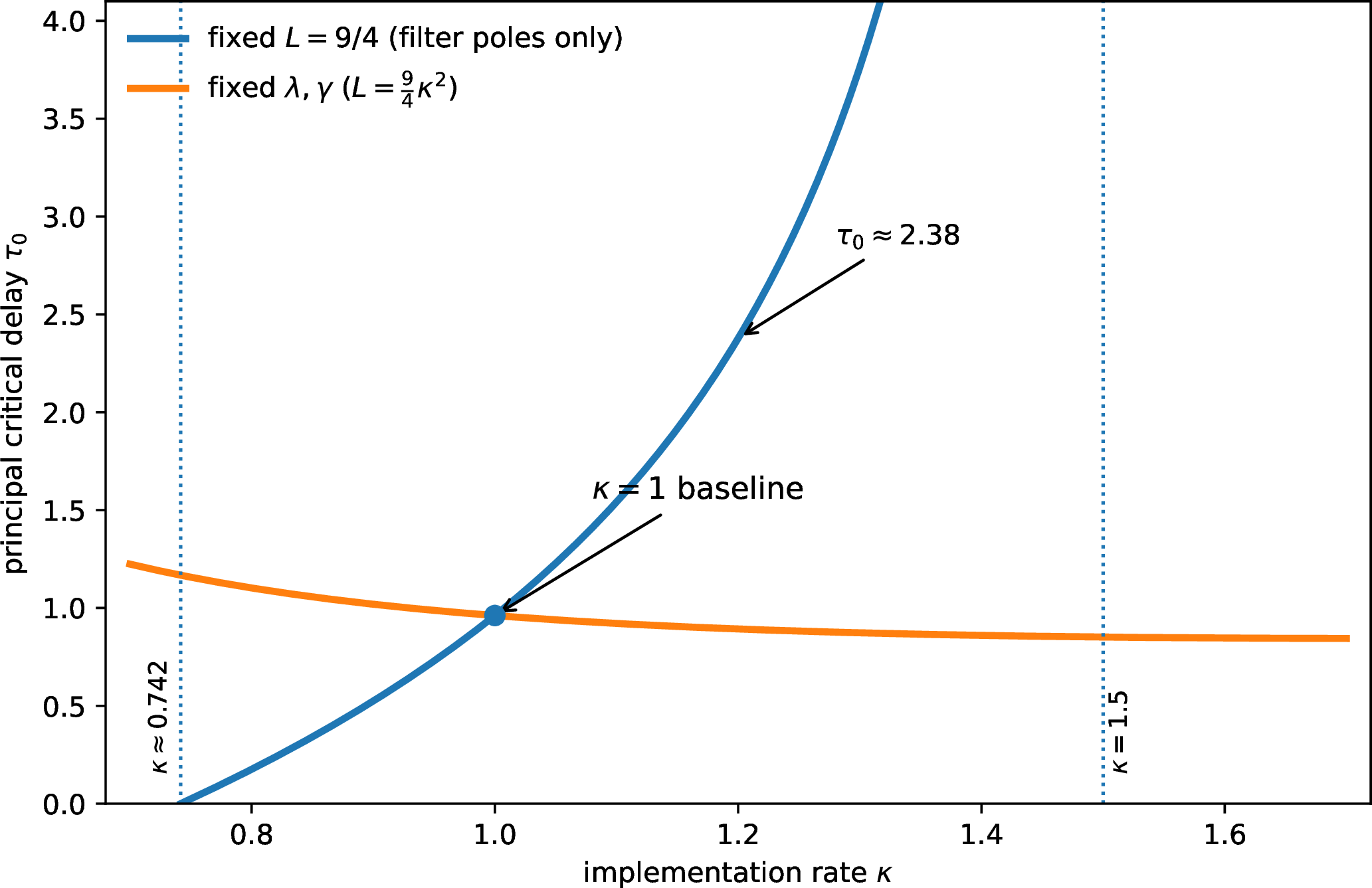
Interpretation. This sweep isolates the filter-pole effect by holding the effective branch strength \(L=K|\gamma|\) fixed, so changing \(\kappa\) moves the real filter poles in \(R(z)\) but not \(L\) itself. Under this convention, moving from \(\kappa=1\) to \(\kappa=1.2\) raises the critical delay from about \(0.96\) to about \(2.38\): at fixed loop gain, faster fielding enlarges the delay margin. The convention matters. If instead the primitive selection rates \(\lambda_X,\lambda_Y\) and the spectral branch \(\gamma\) are held fixed, then the cleared characteristic factor has \(L=K|\gamma|=\tfrac94\kappa^2\), while the filter factors in \(R(z)\) move at the same time; in the plotted range these two effects nearly cancel and the second curve in Figure 2 is almost flat, so merely fielding faster does little to the margin once the simultaneous change in the cleared branch strength is accounted for. The operative quantity is always the branch strength entering the characteristic factor, not the implementation rate in isolation.
6.0.0.4 Diagnostic 3: local normal-form coefficient for the baseline branch
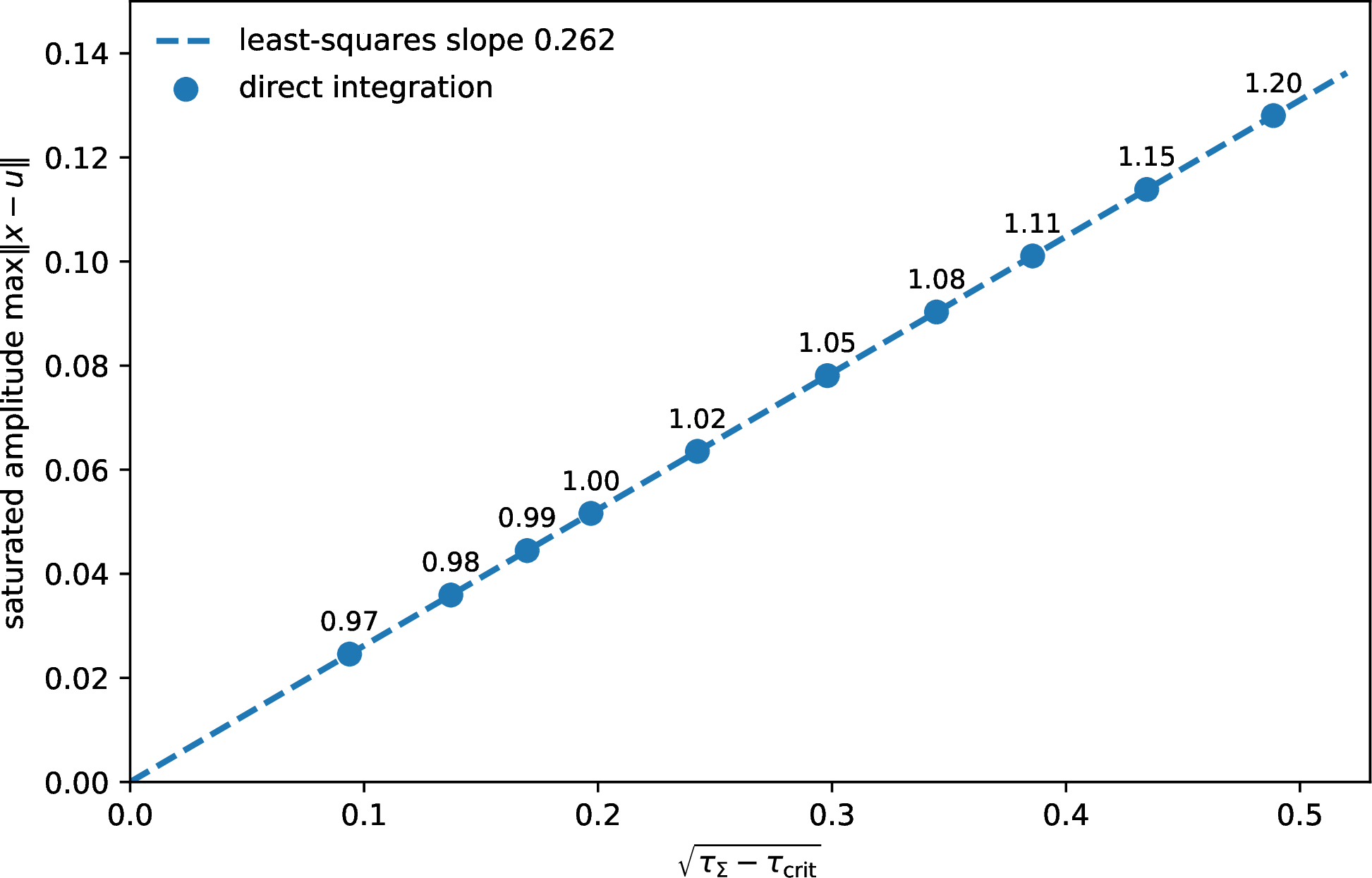
The Hopf theorem of Section 4 gives existence and transversality but not the criticality of the periodic branch. For the baseline branch we compute the cubic Hopf coefficient directly from the finite normal form of the retarded tangent system; the calculation uses the full tangent system, not only the scalar characteristic factor, because the noncritical tangent mode enters the centre-manifold correction at second order. The result, derived in Appendix 12, is \[c_H=-0.9193272749-0.1089995716\,i, \qquad \operatorname{Re}c_H<0,\] so the baseline Hopf bifurcation is supercritical and the small postcritical periodic branch is locally orbitally attracting for \(\tau_\Sigma>\tau_{\rm crit}\). The same coefficient predicts the deployed-amplitude law and nonlinear frequency \[\max\|x-u\|\sim0.26345\,\sqrt{\tau_\Sigma-\tau_{\rm crit}}, \qquad \Omega(\delta)=\omega_\ast-0.1629106770\,\delta+O(\delta^2),\] with \(\beta=0.0797591244\) the transversality coefficient, \(\|q_\xi\|=1/\sqrt5\) the deployed-\(x\) part of the critical eigenvector, and \(\delta=\tau_\Sigma-\tau_{\rm crit}\); at \(\tau_\Sigma=1.10\) the frequency law gives \(T_{\rm comp}\approx9.18\) and \(T_{\rm scalar}\approx4.59\). Both predictions are tested by direct integration below. Along the whole leading branch of the diagonal three-strategy family, Proposition 8 shows that the equal-split Hopf coefficient has negative real part for every \(L\in(1,4)\); Table 5 gives representative Euclidean-normalized values. In the exactly solvable two-strategy case the cubic coefficient is negative in closed form (Proposition 9).
6.0.0.5 Diagnostic 4: direct time-domain integration
We integrate the full nonlinear delay system for the baseline parameters 70 –72 . The total hard delay is split equally across the four channels, \[\sigma_X=\sigma_Y=\theta_X=\theta_Y=\frac{\tau_\Sigma}{4}.\] This split is used only for simulation; the analytical threshold depends on the sum \(\tau_\Sigma\). The initial histories are small tangent perturbations of the barycenter, with all four portfolios in the interior of \(\Delta_3\). Numerical details and a step-refinement check are reported in Appendix 13.
Figure 3 compares two cases. For \(\tau_\Sigma=0.80<\tau_{\rm crit}\), the deployed portfolio returns to the barycenter. For \(\tau_\Sigma=1.10>\tau_{\rm crit}\), the perturbation grows away from the barycenter and, in the displayed integration, settles into a bounded oscillatory regime; the late-time window displays the corresponding periodic motion. By Lemma 4, the leading branch crosses the imaginary axis only at \(\tau_{\rm crit}+2\pi k/\omega_\ast\), and the second branch (\(L_2=9/16<c_\ast\)) never crosses; hence on \((\tau_{\rm crit},\tau_{\rm crit}+2\pi/\omega_\ast)\approx(0.96,9.85)\), in particular at \(\tau_\Sigma=1.10\), the barycenter carries exactly one unstable conjugate pair. Thus the growth away from the barycenter is a genuine linear instability rather than a transient of the chosen observation window; bounded saturation of the nonlinear oscillation is the numerical behavior displayed by the integration.
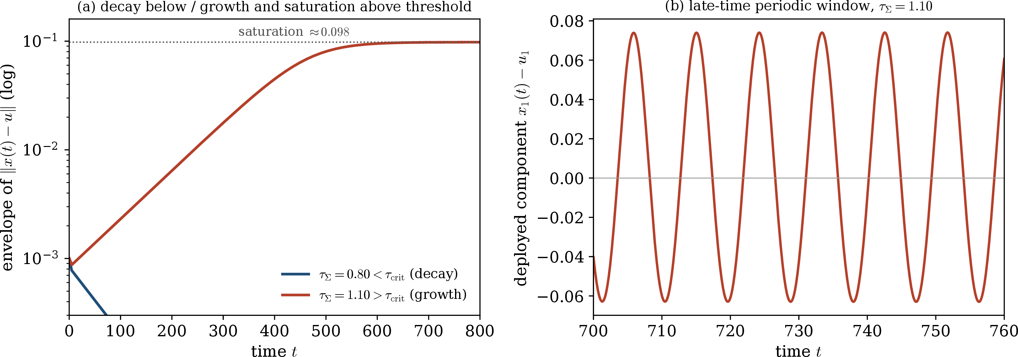
Interpretation. The analytical threshold has the expected time-domain meaning. Below the threshold, a small reshuffle is absorbed and the contest returns to a balanced mixture. Above it, each correction arrives late enough to seed the next counter-correction, and the displayed run enters a back-and-forth regime. This is the numerical analogue of a stable adaptive standoff becoming a self-sustained arms race among methods; global attraction of that finite-amplitude cycle is not claimed.
6.0.0.6 Diagnostic 5: amplitude scaling at onset
The normal-form calculation of Diagnostic 3 predicts the square-root law \(\max\|x-u\|\sim0.26345\sqrt{\tau_\Sigma-\tau_{\rm crit}}\) for the equal-split baseline branch. We test this prediction by integrating the nonlinear system for a range of total delays just above threshold and recording the saturated peak of \(\|x(t)-u\|\). Figure 4 plots the measured amplitude against \(\sqrt{\tau_\Sigma-\tau_{\rm crit}}\). The direct-integration fit is \[\max\|x-u\|\approx0.262\,\sqrt{\tau_\Sigma-\tau_{\rm crit}}, \qquad \text{least squares},\] in close agreement with the normal-form prediction. The numerical saturated cycles are thus consistent with the analytically classified supercritical Hopf onset of the baseline branch.
6.0.0.7 Diagnostic 6: hidden fundamental and scalar second harmonic
Table 2 compares the linear Hopf periods with periods measured from the late-time oscillatory run at \(\tau_\Sigma=1.10\). The measured values are close to, but not identical with, the linear Hopf predictions because the run is not infinitesimally close to the threshold.
| Quantity | Linear Hopf prediction | Measured (simulation) |
|---|---|---|
| Critical delay \(\tau_{\rm crit}\) | \(0.9612\) | – |
| Hopf frequency \(\omega_\ast\) | \(0.7071\) | – |
| Compositional period \(2\pi/\omega_\ast\) | \(8.886\) | \(9.174\) |
| Scalar period \(\pi/\omega_\ast\) | \(4.443\) | \(4.587\) |
Figure 5 shows the observable signature after transients. The first curve is a deployed compositional component, \(x_1(t)-u_1\). The other two curves are the centered scalar performances \(\Phi_X-\overline{\Phi}_X\) and \(\Phi_Y-\overline{\Phi}_Y\), rescaled only for visual comparison.
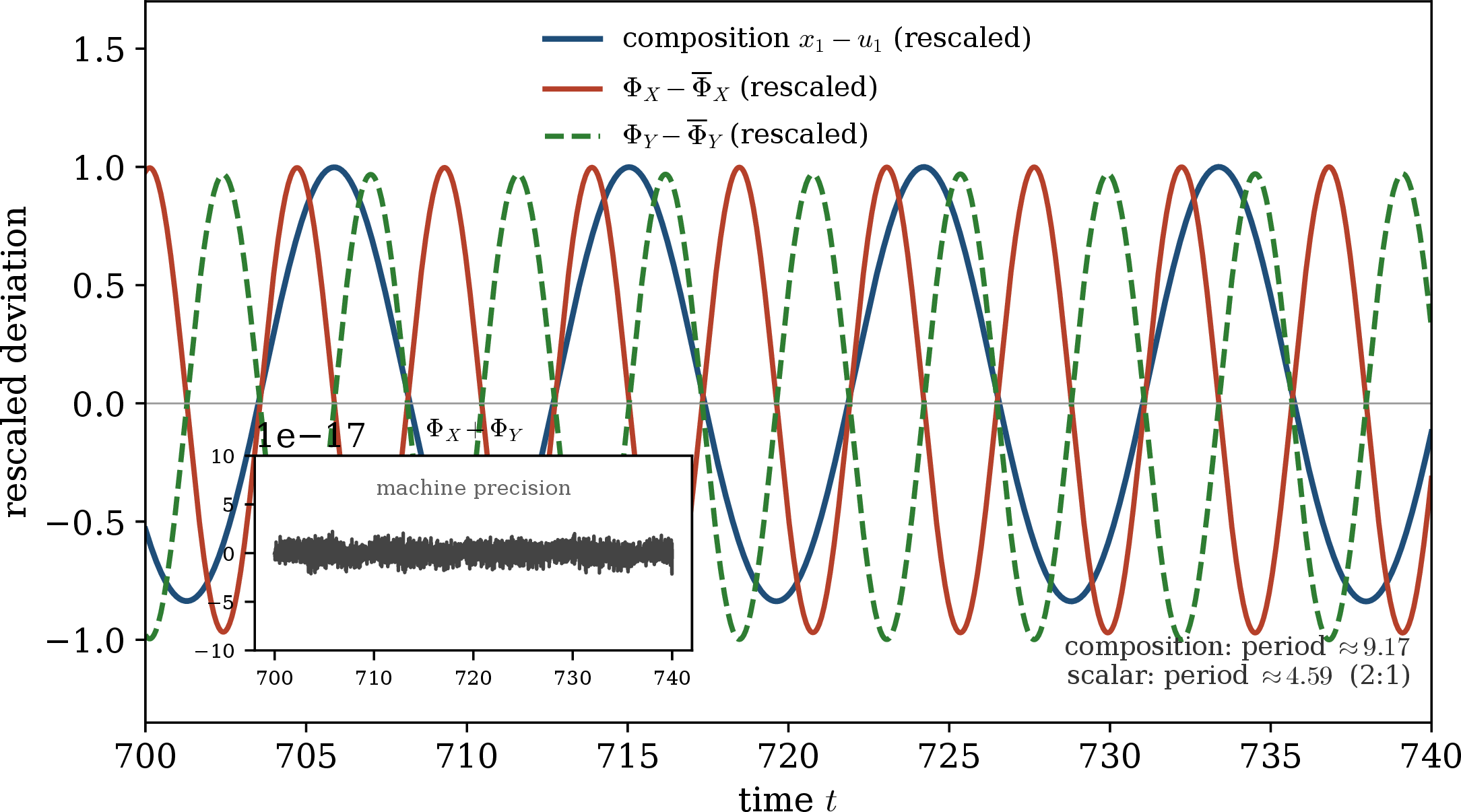
The trace displays the signatures predicted by Corollaries 1 and 4. The portfolio component completes one oscillation over the compositional period, while the scalar performance completes two. Moreover, because \(B=-A^\top\), \[\Phi_Y(t)-\Phi_Y(u,u)=-(\Phi_X(t)-\Phi_X(u,u))\] in this example, so the scalar performance signals are in exact antiphase with equal amplitude.
Interpretation. If only headline effectiveness is observed, the apparent period can be half the period of the hidden portfolio race. If both composition and scalar performance are measured, the frequency-doubling signature tests the balanced core model. The antiphase relation is a sharper test of strict antagonism: it predicts not merely that both sides oscillate, but that their scalar performance deviations are locked with phase difference \(\pi\) and fixed amplitude ratio \(\chi\).
6.0.0.8 Robustness of the antiphase law beyond \(\chi=1\)
The baseline uses \(B=-A^\top\) (\(\chi=1\)), for which Corollary 4 predicts equal-amplitude antiphase. To check that the antiphase amplitude-ratio law is not an artifact of this symmetric case, we repeat the integration for \(\mathcal{B}_\rho=-\chi\mathcal{A}_\rho^\top\) with \(\chi=2,3\), choosing \(\lambda_X=\lambda_Y\) so that the leading branch strength stays at \(L=9/4\); the linear threshold \(\tau_{\rm crit}\approx0.9612\) is therefore unchanged, and the run is again taken at \(\tau_\Sigma=1.10\). Table 3 reports the measured scalar phase shift and the amplitude ratio of \(\Phi_X\) and \(\Phi_Y\). This is a numerical consistency check of the implementation and scaling, not an independent empirical test of the algebraic identity: Corollary 4 predicts the ratio exactly under strict antagonism. In every case the two scalar performances are in antiphase with amplitude ratio \(\chi\), and the affine constraints hold to roundoff.
| \(\chi\) | scalar phase shift | amplitude ratio (measured) | prediction |
|---|---|---|---|
| \(1\) | \(\pi\) | \(1.0000\) | \(1\) |
| \(2\) | \(\pi\) | \(2.0000\) | \(2\) |
| \(3\) | \(\pi\) | \(3.0000\) | \(3\) |
6.0.0.9 Delay allocation at fixed budget
Corollary 3 predicts that the Hopf threshold depends on the hard lags only through their sum, while the split of that sum among the four channels enters the critical eigenvectors rather than the threshold (Section 5). There is, moreover, an exact reason for the reduced revision dynamics to coincide across splits. By the shifted-exponential representation 6 , the opponent’s deployed state seen by the \(X\)-revision, \(y(t-\sigma_X)\), depends on \(q\) only through the hard shift \(\sigma_X+\theta_Y\), and \(x(t-\sigma_Y)\) depends on \(p\) through \(\sigma_Y+\theta_X\). The closed revision dynamics therefore depend on the four hard lags only through the two cross-delays \[\delta_X=\sigma_X+\theta_Y, \qquad \delta_Y=\sigma_Y+\theta_X, \qquad \delta_X+\delta_Y=\tau_\Sigma,\] together with the filter rates. We test this by fixing \(\tau_\Sigma=1.10\) and integrating three allocations: an equal split, an observation-heavy split \((\sigma_X,\sigma_Y;\theta_X,\theta_Y)=(0.5,0.5;0.05,0.05)\), and a deployment-heavy split \((0.05,0.05;0.5,0.5)\). In all three, \(\delta_X=\delta_Y=0.55\). Thus, apart from the prescribed initial history, the reduced revision equations have the same hard-shift structure in all three cases. For compatible histories the reduced revision trajectories are identical, not merely threshold-equivalent. In the simulations below the same late-time attracting regime is reached after transients, and the measured fundamental period is unchanged to the reported precision. The deployed-versus-intended phase, by contrast, is rephased by each side’s own deployment filter: for a periodic revision signal \(p(t)=\sum_{n}p_ne^{in\Omega t}\) the deployment equation gives \(x_n=\kappa_Xe^{-in\Omega\theta_X}p_n/(\kappa_X+in\Omega)\), so the fundamental deployed-versus-intended phase is exactly \(-\Omega\theta_X-\arctan(\Omega/\kappa_X)\), which the measurements reproduce to a fraction of a degree. Shifting the budget toward observation advances the deployed mixture relative to intent; shifting it toward deployment retards it, with the threshold unchanged.
| split | per-side \((\sigma_i,\theta_i)\) | period | \(x_1\) vs.\(p_1\) phase (meas./pred.) |
|---|---|---|---|
| equal | \((0.275,0.275)\) | \(9.17\) | \(-45.2^\circ\,/\,-45.2^\circ\) |
| observation-heavy | \((0.5,0.05)\) | \(9.17\) | \(-36.4^\circ\,/\,-36.4^\circ\) |
| deployment-heavy | \((0.05,0.5)\) | \(9.17\) | \(-54.0^\circ\,/\,-54.0^\circ\) |
6.0.0.10 Summary
The calculations are intentionally small and transparent. They support the diagnostic reading of the analysis: branch strength selects the stability regime, implementation speed is an independent stability lever, and balanced scalar outputs can report a second harmonic rather than the hidden compositional period. For the baseline branch the finite normal-form calculation gives a negative cubic Hopf coefficient, so the onset is supercritical and the small postcritical cycle is locally attracting; the amplitude slope predicted from this coefficient agrees with the direct-integration fit. For general parameter families, however, the theorem of Section 4 asserts only existence and transversality, and criticality must be checked branch by branch. Global continuation of nonlinear periodic branches is a separate problem; no claim in this paper relies on the global behaviour of the nonlinear branch.
7 Discussion↩︎
This paper isolates a mechanism that is missed by a single delayed replicator equation. In the revision–deployment model, deciding and fielding are separate state layers. Observation and hard deployment lags enter the first Hopf threshold through the total hard delay \(\tau_\Sigma\), while implementation rates enter through real filter factors in the loop-transfer representation. Thus stability depends not only on how fast a side selects a new portfolio, but also on how that portfolio becomes deployed capability.
The main practical implication is delay-budget triage. In the delay-induced window, the balanced state is locally stable below the critical total delay and loses stability when the feedback loop becomes too stale. At the branch’s first crossing, all hard-lag components have the same first-order stabilizing leverage: shortening observation, validation, or rollout by the same amount moves the critical root left by the same amount. In the filter-induced regime the diagnosis is different. The instability is at or beyond the zero-hard-delay implementation-filter margin, so improving observation or rollout time alone is not the relevant remedy; the implementation filter, damping, or effective antagonistic branch strength must change.
For the baseline example, the finite Hopf normal-form calculation gives a negative cubic coefficient. Hence the local onset is supercritical and the small postcritical periodic branch is locally orbitally attracting. The predicted amplitude slope agrees with direct integration. This classification is local and branch-specific. The general theorem gives existence and transversality; global attraction of the finite-amplitude cycle displayed at \(\tau_\Sigma=1.10\) is supported by simulation rather than by a global continuation proof.
The second practical implication concerns observability. In the balanced core, portfolio composition oscillates at the Hopf frequency, whereas scalar effectiveness has no linear term and therefore shows a mean shift plus a leading second harmonic. A measured effectiveness cycle of period \(T\) can therefore correspond to a hidden compositional race of period \(2T\). Under strict antagonism the two scalar effectiveness deviations also satisfy \[\Phi_Y-\Phi_Y^\ast=-\chi(\Phi_X-\Phi_X^\ast),\] so their amplitudes have ratio \(\chi\) and their phases are opposed. These are diagnostic signatures of the model class, not policy prescriptions.
The cybersecurity reading is direct: revision is the intended mix of detection rules, patches, configurations, or offensive techniques, while deployment is fielded coverage. Observation delay is the time needed to infer the opponent’s current mix; deployment delay and implementation rate describe how long a validated decision takes to reach the field. The same abstraction applies to rapid uncrewed-system and countermeasure adaptation without making any theatre-specific claim. The model does not identify which method to choose; it identifies which clocks matter.
The assumptions are deliberately restrictive. The mode set is fixed, so the model describes reallocations among already defined methods rather than the birth of new modes. Barycentric balance keeps the equilibrium at the simplex barycenter and makes scalar observables second order; off-center or biased contests can restore first-order scalar signals. The main Hopf theorem is stated for strict antagonism and uniform exploration. Outside that class, complex spectral branches and structured mutation require the full determinant rather than the scalar branch factor. The model is also deterministic and local; it does not include stochastic shocks, spatial logistics, finite inventories, network constraints, or optimal control.
Finally, the model is a relative-composition model, not a victory or cost model. It has no terminal state, no absolute-loss accounting, and no claim about who wins a particular contest. Its contribution is mechanism-level: implementation lag can change which state is stable, when oscillation begins, and what an observer sees. This is the coevolutionary analogue of the author’s earlier implementation-lag threshold mechanism, where restoration was preventive rather than curative. Here the corresponding message is that oscillation management is delay-budget triage.
In summary, the model gives four testable diagnostics: the onset of oscillation is governed by total hard feedback lag in the delay-induced regime; fielding speed is an independent stability lever through implementation filters; balanced scalar effectiveness can report a second harmonic rather than the hidden compositional period; and strict antagonism locks the two scalar effectiveness signals in antiphase with fixed amplitude ratio.
8 Details for Section 2↩︎
8.0.0.1 Proof of Proposition 1
We give the argument for \(p\) and \(x\); the other variables are identical. Let \(s_p(t)=\mathbf{1}^\top p(t)\). Since \(\mathbf{1}^\top M_X=\mathbf{1}^\top\), summing 1 gives \[\dot{s}_p(t)=\lambda_Xp(t)^\top f_X^\sigma(t)[1-s_p(t)].\] Thus \(s_p(0)=1\) implies \(s_p(t)=1\). If \(p_k(t)=0\), the replicator term in the \(k\)-th component vanishes and \(\dot{p}_k=\mu_X(M_Xp)_k\ge0\). Hence the nonnegative orthant is invariant; strict positivity follows for strictly positive \(M_X\), and in the uniform case \((M_Xp)_k=1/m\).
For deployment, summing 3 gives \(\frac{d}{dt}\mathbf{1}^\top x=\kappa_X(1-\mathbf{1}^\top x)\). Nonnegativity follows from the variation-of-constants formula 5 : it expresses \(x(t)\) as a convex combination of \(x(0)\) and delayed values of \(p\), all in \(\Delta_m\). Therefore \(x(t)\in\Delta_m\).
8.0.0.2 Derivation of the characteristic factors
Substituting \(\alpha=ae^{zt}\), \(\beta=be^{zt}\), \(\xi=re^{zt}\), \(\eta=se^{zt}\) into 17 –18 gives \[(zI-\mathcal{L}_X)a=\frac{\lambda_X}{m}\mathcal{A}_\rho s e^{-z\sigma_X}, \quad (zI-\mathcal{L}_Y)b=\frac{\lambda_Y}{m}\mathcal{B}_\rho r e^{-z\sigma_Y},\] \[(z+\kappa_X)r=\kappa_Xae^{-z\theta_X}, \quad (z+\kappa_Y)s=\kappa_Ybe^{-z\theta_Y}.\] Eliminating \(r,s\) gives 20 . In the uniform case, \(\mathcal{L}_X=-\mu_XI\), \(\mathcal{L}_Y=-\mu_YI\). Eliminating \(b\) gives \[(z+\mu_X)(z+\mu_Y)(z+\kappa_X)(z+\kappa_Y)a =Ke^{-z\tau_\Sigma}\mathcal{A}_\rho\mathcal{B}_\rho a,\] which is 21 and 23 .
8.0.0.3 Proof of Lemma 1
At zero delay the scalar branch is \[z^4+c_3z^3+c_2z^2+c_1z+c_0=0, \qquad c_0=c_\ast-\Gamma_\rho.\] The Routh–Hurwitz conditions for a quartic are \(c_3,c_2,c_1,c_0>0\), \(c_3c_2-c_1>0\), and \((c_3c_2-c_1)c_1>c_3^2c_0\). For positive \(r_i\), the first three inequalities and \(c_3c_2-c_1>0\) are automatic. The two remaining conditions are exactly 24 –25 .
8.0.0.4 Proof of Corollary 1
By 10 , the leading variation is \(\xi^\top A_\rho\eta\). With \[\xi=\varepsilon\operatorname{Re}(ve^{i\omega_\ast t})+\mathcal{O}(\varepsilon^2), \quad \eta=\varepsilon\operatorname{Re}(we^{i\omega_\ast t})+\mathcal{O}(\varepsilon^2),\] a direct multiplication gives \[\xi^\top A_\rho\eta =\frac{\varepsilon^2}{2}\operatorname{Re}(v^\top A_\rho\overline{w}) +\frac{\varepsilon^2}{2}\operatorname{Re}(v^\top A_\rho w e^{2i\omega_\ast t}) +\mathcal{O}(\varepsilon^3).\] The formula for \(Y\) is identical.
9 Details for Section 3↩︎
9.0.0.1 Proof of Proposition 3
We prove the identity for \(X\); the proof for \(Y\) is identical. Set \[f_X(t)=A_\rho y(t),\qquad f_X^\sigma(t)=A_\rho y(t-\sigma_X),\] so that \(\overline{F}_X(t)=p(t)^\top f_X(t)\). Differentiating gives \[\frac{d}{dt}\overline{F}_X(t)=\dot{p}(t)^\top f_X(t)+p(t)^\top A_\rho\dot{y}(t).\] The selection part of \(\dot{p}\) contributes \[\begin{align} &\lambda_X\left[p\odot\left(f_X^\sigma-(p^\top f_X^\sigma)\mathbf{1}\right)\right]^\top f_X \\ &\quad=\lambda_X\left[p^\top(f_X^\sigma\odot f_X)-(p^\top f_X^\sigma)(p^\top f_X)\right] =\lambda_X\operatorname{Cov}_{p(t)}(f_X(t),f_X^\sigma(t)). \end{align}\] The mutation part gives \(\mu_X(M_Xp-p)^\top f_X\), and the deployment equation gives \[p^\top A_\rho\dot{y}=\kappa_Yp^\top A_\rho[q(t-\theta_Y)-y(t)].\] Combining these terms yields ?? .
9.0.0.2 Proof of Corollary 2
Set \[g(t)=\mathcal{A}_\rho\eta(t),\qquad h(t)=\mathcal{A}_\rho\eta(t-\sigma_X).\] By barycentric balance, \(g,h\in T\Delta_m\) and \(u^\top g=u^\top h=0\). Since constants do not affect covariance, \[\operatorname{Cov}_{u+\alpha}(a_\rho\mathbf{1}+g,a_\rho\mathbf{1}+h) = (u+\alpha)^\top(g\odot h)-[(u+\alpha)^\top g][(u+\alpha)^\top h].\] Now \((u+\alpha)^\top(g\odot h)=m^{-1}g^\top h+\mathcal{O}(\|(\alpha,\eta)\|^3)\) and \([(u+\alpha)^\top g][(u+\alpha)^\top h]=\mathcal{O}(\|(\alpha,\eta)\|^4)\). This proves 29 . The \(Y\) identity is analogous.
9.0.0.3 Hopf-mode covariance expansion
If \[\eta(t)=\varepsilon\operatorname{Re}(w e^{i\omega_\ast t})+\mathcal{O}(\varepsilon^2),\] then 29 gives \[\begin{align} &\operatorname{Cov}_{p(t)}\left(A_\rho y(t),A_\rho y(t-\sigma_X)\right) \\ &\quad = \frac{\varepsilon^2}{2m}\operatorname{Re} \left[(\mathcal{A}_\rho w)^\top\overline{\mathcal{A}_\rho w}\,e^{i\omega_\ast\sigma_X}\right] + \frac{\varepsilon^2}{2m}\operatorname{Re} \left[(\mathcal{A}_\rho w)^\top(\mathcal{A}_\rho w)e^{2i\omega_\ast t-i\omega_\ast\sigma_X}\right] +\mathcal{O}(\varepsilon^3). \end{align} \label{eq:covariance-hopf-mode-X}\tag{74}\] Since \((\mathcal{A}_\rho w)^\top\overline{\mathcal{A}_\rho w}=\|\mathcal{A}_\rho w\|^2\ge0\), the first term is a delay-dependent mean contribution proportional to \(\|\mathcal{A}_\rho w\|^2\cos(\omega_\ast\sigma_X)\), while the second term is a second harmonic.
9.0.0.4 Deployment performance identity
For \(\Phi_X(t)=x(t)^\top A_\rho y(t)\), the deployment equations give \[\begin{align} \dot{\Phi}_X(t) &=\dot{x}(t)^\top A_\rho y(t)+x(t)^\top A_\rho\dot{y}(t) \\ &=\kappa_X\left[p(t-\theta_X)^\top A_\rho y(t)-\Phi_X(t)\right] +\kappa_Y\left[x(t)^\top A_\rho q(t-\theta_Y)-\Phi_X(t)\right]. \end{align} \label{eq:deployed-performance-identity-X}\tag{75}\] Similarly, \[\dot{\Phi}_Y(t) =\kappa_Y\left[q(t-\theta_Y)^\top B_\rho x(t)-\Phi_Y(t)\right] +\kappa_X\left[y(t)^\top B_\rho p(t-\theta_X)-\Phi_Y(t)\right]. \label{eq:deployed-performance-identity-Y}\tag{76}\]
10 Details for Section 4↩︎
10.0.0.1 Proof of Lemma 2
Only the secant bound needs proof, since the Routh–Hurwitz part of the zero-delay margin was given in Appendix 8. For the negative branch at zero hard delay, \[R(z)+L=0,\] the Routh–Hurwitz boundary is \(L=H-c_\ast\). At this boundary there is a simple imaginary pair. Indeed, for \[z^4+c_3z^3+c_2z^2+c_1z+c_0\] the imaginary part at \(z=i\omega\) is \(\omega(c_1-c_3\omega^2)\), hence \[\omega_0^2=\frac{c_1}{c_3}.\] The real part then vanishes precisely when \[c_0=c_2\omega_0^2-\omega_0^4 =\frac{(c_3c_2-c_1)c_1}{c_3^2}=H.\] At the boundary the quartic factors as \[(z^2+\omega_0^2)\left(z^2+c_3z+\frac{H}{\omega_0^2}\right),\] and the remaining quadratic has positive coefficients. Thus the boundary carries the simple pair \(z=\pm i\omega_0\) and the other roots remain in the left half-plane.
At this boundary, \[R(i\omega_0)+L=0, \qquad \sum_{j=1}^4\arctan\frac{\omega_0}{r_j}=\pi.\] Set \[\theta_j=\arctan\frac{\omega_0}{r_j}\in(0,\pi/2).\] Then \(\sum_j\theta_j=\pi\) and \[\frac{H-c_\ast}{c_\ast} =\frac{L}{c_\ast} =\frac{|R(i\omega_0)|}{R(0)} =\prod_{j=1}^4\sqrt{1+\left(\frac{\omega_0}{r_j}\right)^2} =\prod_{j=1}^4\sec\theta_j.\] Since \(\log\sec\theta\) is strictly convex on \((0,\pi/2)\), Jensen’s inequality gives \[\frac{1}{4}\sum_{j=1}^4\log\sec\theta_j \ge \log\sec\left(\frac{1}{4}\sum_{j=1}^4\theta_j\right) =\log\sec\frac{\pi}{4}.\] Therefore \[\prod_{j=1}^4\sec\theta_j\ge \sec^4\frac{\pi}{4}=4.\] This proves \(H-c_\ast\ge4c_\ast\), or \(H\ge5c_\ast\). Equality holds if and only if \(\theta_1=\cdots=\theta_4=\pi/4\), equivalently \(r_1=\cdots=r_4\).
10.0.0.2 Proof of Lemma 3
For the negative branch, set \[F(z,\tau)=R(z)+Le^{-z\tau}.\] At a root, \(Le^{-z\tau}=-R(z)\). Differentiating implicitly gives \[F_z\frac{dz}{d\tau}+F_\tau=0.\] Moreover, \[F_z=R'(z)-\tau Le^{-z\tau}=R'(z)+\tau R(z), \qquad F_\tau=-zLe^{-z\tau}=zR(z).\] Hence \[\frac{dz}{d\tau} =-\frac{F_\tau}{F_z} =-\frac{zR(z)}{R'(z)+\tau R(z)} =-\frac{z}{R'(z)/R(z)+\tau}.\] At \(z=i\omega_\ast\), use \[\frac{R'(i\omega)}{R(i\omega)}=a(\omega)-ib(\omega)\] to obtain \[\frac{dz}{d\tau} =-\frac{i\omega_\ast}{a(\omega_\ast)+\tau-ib(\omega_\ast)}.\] Taking the real part gives 47 , which is strictly positive because \(\omega_\ast>0\) and \(b(\omega_\ast)>0\).
10.0.0.3 Proof of Theorem 5
In the strictly antagonistic class, \(\mathcal{C}_\rho=-\chi\mathcal{A}_\rho\mathcal{A}_\rho^\top\) is symmetric nonpositive on \(T\Delta_m\). Hence all spectral branches are real and nonpositive. Zero branches contribute only the stable roots \(-r_j\), and all possible oscillatory branches are the negative branches treated in Section 4.
By hypothesis, the zero-hard-delay equilibrium is asymptotically stable. Since the characteristic equation is retarded, characteristic roots depend continuously on \(\tau\), and stability can be lost only through imaginary-axis crossings. A negative branch has a positive-frequency imaginary root only when \(L(\gamma)>c_\ast\), and it is zero-hard-delay stable only when \(L(\gamma)<H-c_\ast\). Therefore every possible delay-induced crossing is included in the minimization 49 ; branches outside that window either have no positive-frequency crossing or are already unstable at zero hard delay.
The simplicity assumption isolates a single critical spectral branch and a single root pair. No other root lies on the imaginary axis at \(\tau=\tau_{\rm crit}\) by hypothesis. Lemma 3 gives a nonzero crossing speed, with the root pair crossing from left to right as \(\tau\) increases. The Hopf bifurcation theorem for retarded functional differential equations [24], [25] then yields a local branch of periodic solutions. Its criticality and orbital stability are governed by the first Lyapunov coefficient, computed for the baseline branch in Appendix 12.
11 Details for Section 5↩︎
11.0.0.1 Proof of Proposition 7
Differentiating \(\log|R(i\omega)|\) gives \[\frac{d}{d\omega}\log|R(i\omega)| =\sum_{j=1}^4\frac{\omega}{r_j^2+\omega^2}=b(\omega)>0,\] so the defining relation 56 , \(|R(i\omega_\ast)|=L\), yields \[\frac{d\omega_\ast}{dL}=\frac{1}{L\,b(\omega_\ast)}.\] Differentiating \(\tau_0=(\pi-\phi(\omega))/\omega\) and using \(\phi'(\omega)=a(\omega)\), \[\frac{d}{d\omega}\!\left(\frac{\pi-\phi(\omega)}{\omega}\right) =-\frac{\omega\,a(\omega)+\pi-\phi(\omega)}{\omega^2}.\] Combining the two identities gives ?? . Inside the delay-induced window \(c_\ast<L<H-c_\ast\) one has \(0<\phi(\omega_\ast)<\pi\) and \(a(\omega_\ast),b(\omega_\ast)>0\), so numerator and denominator are both positive and \(d\tau_0/dL<0\).
12 Hopf criticality of the baseline branch↩︎
This appendix records the finite normal-form calculation that classifies the baseline Hopf point, together with its consequences for the amplitude and frequency of the postcritical cycle. The calculation is for the equal-split baseline \[\sigma_X=\sigma_Y=\theta_X=\theta_Y=\frac{\tau_{\rm crit}}{4},\] with the matrices and rates in Appendix 13. The critical frequency and total hard delay are \(\omega_\ast=0.7071067812\) and \(\tau_{\rm crit}=0.9612039327\), and the transversality coefficients are \[\beta=\left.\frac{d\operatorname{Re}z}{d\tau_\Sigma}\right|_{\tau_{\rm crit}}=0.0797591244, \qquad \nu=\left.\frac{d\operatorname{Im}z}{d\tau_\Sigma}\right|_{\tau_{\rm crit}}=-0.1534540769.\]
We use tangent coordinates in the orthonormal basis \((q_1,q_2)\), with state ordering \[(\alpha_1,\alpha_2,\beta_1,\beta_2,\xi_1,\xi_2,\eta_1,\eta_2),\] where \(\alpha,\beta\) are the revision tangents and \(\xi,\eta\) the deployment tangents. A Euclidean-normalized critical right eigenvector is \[q=\sqrt{\tfrac{3}{10}}\left(1,0,\;i,0,\;\tfrac{1-i}{\sqrt3},0,\;\tfrac{1+i}{\sqrt3},0\right)^\top,\] so that \(\|q\|_2=1\) and the deployed-\(x\) part has \(\|q_\xi\|=1/\sqrt5\). Let \[D=\operatorname{diag}(1,1/2),\qquad \lambda=\frac{9}{2}, \qquad \delta=\frac{\tau_{\rm crit}}{4} .\] In the state ordering \[(\alpha_1,\alpha_2,\beta_1,\beta_2,\xi_1,\xi_2,\eta_1,\eta_2),\] the equal-split linear part has characteristic matrix \[M(z)=(z+1)I-\mathcal{L}_1e^{-z\delta},\] where the delayed-coupling matrix is the \(2\times2\) block matrix \[\mathcal{L}_1= \begin{pmatrix} 0&0&0&\frac{3}{2}D\\ 0&0&-\frac{3}{2}D&0\\ I&0&0&0\\ 0&I&0&0 \end{pmatrix}.\] Let \(p\) be the adjoint eigenvector normalized by \[p^\ast M'(i\omega_\ast)q=1.\] With this normalization, \[\begin{align} p={}&(0.3612241965+0.0494869053i,\;0,\; -0.0494869053+0.3612241965i,\;0,\;\\ &\quad 0.3556862478-0.2699724135i,\;0,\; 0.2699724135+0.3556862478i,\;0)^\top . \end{align}\] This gives \(p^\ast M'(i\omega_\ast)q=1\) to the displayed precision.
The nonlinear tangent term used in the normal-form calculation is also explicit. For \(a=(a,b)\) and delayed opponent deployment \(g=(g,h)\), define \[\mathcal{N}(a,b;g,h)= \begin{pmatrix} \dfrac{\sqrt6}{12}(ah+2bg)-a^2g-\dfrac12abh\\[0.7em] \dfrac{\sqrt6}{6}ag-\dfrac{\sqrt6}{12}bh-abg-\dfrac12b^2h \end{pmatrix}.\] Then the nonlinear part of the \(X\)-revision equation is \[\lambda\,\mathcal{N}(\alpha_1,\alpha_2;\eta_1(t-\delta),\eta_2(t-\delta)),\] and, because \(B=-A\), the nonlinear part of the \(Y\)-revision equation is \[-\lambda\,\mathcal{N}(\beta_1,\beta_2;\xi_1(t-\delta),\xi_2(t-\delta)).\] The deployment equations have no nonlinear part.
Writing the centre-manifold expansion \[X(t)=Zqe^{i\omega_\ast t}+\overline{Z}\,\overline{q}e^{-i\omega_\ast t} +Z^2h_{20}e^{2i\omega_\ast t}+Z\overline{Z}\,h_{11} +\overline{Z}^2\overline{h}_{20}e^{-2i\omega_\ast t}+\cdots,\] the second-order corrections solve \[M(2i\omega_\ast)h_{20}=N_{20}, \qquad M(0)h_{11}=N_{11},\] where \(N_{20}\) and \(N_{11}\) are the \(Z^2e^{2i\omega_\ast t}\) and \(Z\overline{Z}\) coefficients of the quadratic part of the tangent vector field evaluated on the critical mode. For the baseline values, \[\begin{align} h_{20}={}&(0,\,0.2952741725-0.0869854838i,\,0,\,-0.1706761365+0.1067427373i,\\ &\quad\;\, 0,\,-0.0019274088-0.1777096570i,\,0,\,0.0324823533+0.1115930788i)^\top, \end{align}\] \[h_{11}=(0,\,0.8230285536,\,0,\,0.1175755077,\,0,\,0.8230285536,\,0,\,0.1175755077)^\top.\] Both lie in the noncritical tangent direction \(q_2\): the critical mode sits in \(q_1\), and the simplex nonlinearity couples \(q_1\) into \(q_2\) at second order. Collecting the resonant \(Z^2\overline{Z}e^{i\omega_\ast t}\) coefficient of the cubic part, corrected by the quadratic interaction with \(h_{20}\) and \(h_{11}\), gives \[G_{21}=(-0.6766549711-0.1090984654i,\,0,\,0.5293334015-1.7809136692i,\,0,0,0,0,0)^\top,\] and the cubic Hopf coefficient is \[c_H=p^\ast G_{21}=-0.9193272749-0.1089995716\,i.\] The local Hopf normal form is \[\dot{Z}=\bigl[(\beta+i\nu)(\tau_\Sigma-\tau_{\rm crit})+i\omega_\ast\bigr]Z +c_HZ|Z|^2 +\mathcal{O}\!\left(|Z|^4+|\tau_\Sigma-\tau_{\rm crit}|\,|Z|^2\right).\] Since \(\operatorname{Re}c_H<0\), the baseline Hopf bifurcation is supercritical and the small postcritical periodic branch is locally orbitally attracting for \(\tau_\Sigma>\tau_{\rm crit}\).
On that branch \(|Z|^2=-(\beta/\operatorname{Re}c_H)(\tau_\Sigma-\tau_{\rm crit})+O((\tau_\Sigma-\tau_{\rm crit})^2)\), so, writing \(\delta=\tau_\Sigma-\tau_{\rm crit}\), the deployed amplitude and nonlinear frequency are \[\begin{align} \max\|x-u\| &=2\|q_\xi\|\sqrt{\frac{\beta}{-\operatorname{Re}c_H}}\, \sqrt{\delta} +o\!\left(\sqrt{\delta}\right) =0.26345\,\sqrt{\delta}+o\!\left(\sqrt{\delta}\right),\\ \Omega(\delta) &=\omega_\ast+\Bigl(\nu-\frac{\operatorname{Im}c_H}{\operatorname{Re}c_H}\,\beta\Bigr)\delta+O(\delta^2) =\omega_\ast-0.1629106770\,\delta+O(\delta^2). \end{align}\] At \(\tau_\Sigma=1.10\) this gives \(T_{\rm comp}=2\pi/\Omega\approx9.18\) and \(T_{\rm scalar}\approx4.59\), matching the direct integration (Table 6); the predicted amplitude slope \(0.26345\) agrees with the direct-integration fit \(0.262\) of Figure 4.
12.0.0.1 Reproducibility of the normal-form coefficients
The calculation above is a finite harmonic-balance computation for a retarded delay system with polynomial nonlinearity. The delayed arguments contribute the phase factor \(e^{-in\omega_\ast\delta}\) to the \(n\)-th harmonic. Thus \(N_{20}\) and \(N_{11}\) are obtained by collecting the \(Z^2e^{2i\omega_\ast t}\) and \(Z\overline{Z}\) coefficients of the explicit quadratic field \(\mathcal{N}\) evaluated on \[Zqe^{i\omega_\ast t}+\overline{Z}\,\overline{q} e^{-i\omega_\ast t}\] and its delayed image. The vectors \(h_{20}\) and \(h_{11}\) are then obtained from \[M(2i\omega_\ast)h_{20}=N_{20}, \qquad M(0)h_{11}=N_{11}.\] Finally, \(G_{21}\) is the \(Z^2\overline{Z} e^{i\omega_\ast t}\) coefficient of the cubic field plus the quadratic interactions with \(h_{20}\) and \(h_{11}\), and \[c_H=p^\ast G_{21}.\] Thus the coefficient is obtained by finite-dimensional operations displayed in this appendix: the characteristic matrix \(M(z)\), the nonlinear polynomial \(\mathcal{N}\), the normalized adjoint vector \(p\), the correction vectors \(h_{20},h_{11}\), and the resonant vector \(G_{21}\) are all given explicitly. The numerical rounding in the displayed value of \(c_H\) reflects only the finite-dimensional linear solves and decimal display precision of these quantities.
12.0.0.2 Supercriticality across the leading-branch family
For the diagonal three-strategy family used in Figure 1, the leading-branch criticality can be classified analytically throughout the delay-induced window under the equal hard-lag split. This is not a numerical sweep and not a universal strict-antagonism theorem: it is a sign calculation for this particular diagonal \(m=3\) family. The representative values in Table 5 are reported only as numerical checks of the formula.
Proposition 8 (supercriticality of the leading branch in the diagonal three-strategy example). Consider the diagonal three-strategy family \[A=Q\operatorname{diag}(1,1/2)Q^\top, \qquad B=-A,\] with unit rates \[\mu_X=\mu_Y=\kappa_X=\kappa_Y=1.\] Let the leading antagonistic branch have strength \[L=(1+\omega^2)^2, \qquad 0<\omega<1,\] and choose \(\lambda_X=\lambda_Y=3\sqrt L\). Let the hard lags be split equally, \[\sigma_X=\sigma_Y=\theta_X=\theta_Y=\delta, \qquad \delta=\frac{\tau_0(L)}{4}= \frac{\pi-4\arctan\omega}{4\omega}.\] Then the Hopf bifurcation of the leading branch at \(\tau_\Sigma=\tau_0(L)\) is supercritical for every \(L\in(1,4)\). The small postcritical periodic branch is locally orbitally attracting for \(\tau_\Sigma>\tau_0(L)\) sufficiently close to the threshold.
Proof. Use tangent coordinates in the basis \((q_1,q_2)\), and write the state as \((\alpha_1,\alpha_2,\beta_1,\beta_2,\xi_1,\xi_2,\eta_1,\eta_2)\). In these coordinates the critical leading mode lies in the first tangent direction, whereas the second tangent direction is noncritical and enters through the second-order centre-manifold corrections. With the critical-amplitude normalization \[\alpha_1(t)=Ze^{i\omega t}+\overline{Z} e^{-i\omega t}+\cdots,\] one obtains the cubic coefficient by the same finite calculation as in the baseline appendix: solve \[M(2i\omega)h_{20}=N_{20}, \qquad M(0)h_{11}=N_{11},\] then project the resonant \(Z^2\overline{Z} e^{i\omega t}\) coefficient onto the adjoint critical eigenvector normalized by \(p^\ast M'(i\omega)q=1\). Eliminating \(h_{20}\) and \(h_{11}\) gives the following explicit real part: \[\operatorname{Re}\widetilde{c}_H(\omega) = -\frac{3\,[\delta P_1(\omega)+P_0(\omega)]}{4(\omega^4+2\omega^2+5) (\delta^2\omega^2+\delta^2+2\delta+1) P_-(\omega)P_+(\omega)},\] where \[\begin{align} P_1(\omega)={}&10595\omega^{18}+81273\omega^{16} +256824\omega^{14}+510056\omega^{12}\\ &+635430\omega^{10}+516306\omega^8 +244352\omega^6+64320\omega^4\\ &+8895\omega^2+525, \end{align}\] \[\begin{align} P_0(\omega)={}&33017\omega^{16}+145556\omega^{14} +357512\omega^{12}+491908\omega^{10}\\ &+433170\omega^8+217660\omega^6 +60000\omega^4+8620\omega^2+525, \end{align}\] and \[P_\pm(\omega)=65\omega^6\pm48\omega^5+99\omega^4 \pm16\omega^3+39\omega^2+5.\] For \(0<\omega<1\), one has \(\delta>0\). The polynomials \(P_0\) and \(P_1\) have strictly positive coefficients, hence \(\delta P_1(\omega)+P_0(\omega)>0\). The factors \(\omega^4+2\omega^2+5\) and \(\delta^2\omega^2+\delta^2+2\delta+1\) are also positive. Moreover, \(P_+(\omega)>0\), and \[\begin{align} P_-(\omega) &=65\omega^6-48\omega^5+99\omega^4-16\omega^3+39\omega^2+5\\ &=\omega^4(65\omega^2-48\omega+9) +\omega^2(90\omega^2-16\omega+39)+5. \end{align}\] The two displayed quadratics have negative discriminant and positive leading coefficient, so they are positive for all real \(\omega\). Therefore \(P_-(\omega)>0\), and every factor in the denominator is positive while the formula carries an overall minus sign. Thus \[\operatorname{Re}\widetilde{c}_H(\omega)<0, \qquad 0<\omega<1.\] The Hopf crossing is transverse by Lemma 3, so the Hopf bifurcation is supercritical. A positive real rescaling of the critical amplitude changes the cubic coefficient by a positive factor and does not change the sign of its real part; hence the conclusion is independent of the normalization used to report the numerical coefficients in Table 5. ◻
Table 5 reports representative Euclidean-normalized values of the same cubic coefficient. The values are not used as a proof of the sign; they are a numerical check on the finite normal-form calculation and show that the baseline value \(L=9/4\) is not exceptional. The statement is specific to the equal split: the linear threshold depends only on the total hard delay, but the nonlinear Hopf coefficient can depend on how that total is distributed among the observation and deployment channels.
| \(L\) | \(1.01\) | \(1.10\) | \(1.50\) | \(2.25\) | \(3.00\) | \(3.90\) |
|---|---|---|---|---|---|---|
| \(\omega_\ast\) | \(0.071\) | \(0.221\) | \(0.474\) | \(0.707\) | \(0.856\) | \(0.987\) |
| \(\operatorname{Re}c_H\) | \(-0.071\) | \(-0.229\) | \(-0.551\) | \(-0.919\) | \(-1.168\) | \(-1.376\) |
12.0.0.3 Exactly solvable two-strategy case
When \(m=2\) the tangent space is one-dimensional and the calculation is closed form, providing an analytic family of supercritical Hopf points.
Proposition 9 (supercriticality in the two-strategy symmetric case). Consider the two-strategy strictly antagonistic model with uniform exploration and unit rates \(\mu_X=\mu_Y=\kappa_X=\kappa_Y=1\). Let the leading tangent branch have strength \(L\in(1,4)\), set \[\omega=\sqrt{\sqrt L-1}, \qquad \tau_0(L)=\frac{\pi-4\arctan\omega}{\omega}, \qquad \delta=\frac{\tau_0(L)}{4},\] and split the hard lags equally. Then the Hopf bifurcation at \(\tau_\Sigma=\tau_0(L)\) is supercritical. In the critical coordinate normalized so that \(\alpha(t)=Ze^{i\omega t}+\overline{Z}e^{-i\omega t}+\cdots\), the cubic Hopf coefficient is \[c_H^{(2)}=-\frac{3+i\omega}{1+\delta+i\delta\omega}, \qquad \operatorname{Re}c_H^{(2)} =-\frac{3(1+\delta)+\delta\omega^2}{(1+\delta)^2+\delta^2\omega^2}<0 .\] Hence the small postcritical periodic branch is locally orbitally attracting for \(\tau_\Sigma>\tau_0(L)\) sufficiently close to \(\tau_0(L)\).
Proof. In the one-dimensional tangent coordinates \((\alpha,\beta,\xi,\eta)\), and with the equal split \(\sigma_X=\sigma_Y=\theta_X=\theta_Y=\delta\), the system is \[\dot{\alpha}=-\alpha+\sqrt L\,\eta(t-\delta) -2\sqrt L\,\alpha(t)^2\eta(t-\delta),\] \[\dot{\beta}=-\beta-\sqrt L\,\xi(t-\delta) +2\sqrt L\,\beta(t)^2\xi(t-\delta),\] \[\dot{\xi}=\alpha(t-\delta)-\xi, \qquad \dot{\eta}=\beta(t-\delta)-\eta .\] The two-strategy simplex saturation produces no quadratic tangent monomials. Consequently the second-order centre-manifold corrections vanish: \[h_{20}=h_{11}=0.\] The characteristic matrix is \[M(z)=(z+1)I-e^{-z\delta} \begin{pmatrix} 0&0&0&\sqrt L\\ 0&0&-\sqrt L&0\\ 1&0&0&0\\ 0&1&0&0 \end{pmatrix}.\] At the Hopf point \(L=(1+\omega^2)^2\) and \(\omega\delta=\pi/4-\arctan\omega\). A right critical eigenvector can be chosen as \[q=\left(1,\;i,\;\frac{e^{-i\pi/4}}{\sqrt{1+\omega^2}},\; \frac{i e^{-i\pi/4}}{\sqrt{1+\omega^2}}\right)^\top .\] Let \(\ell\) be a left eigenvector satisfying \(\ell^\top M(i\omega)=0\). A direct multiplication gives the normalization factor \[\ell^\top M'(i\omega)q=4(1+\delta+i\delta\omega).\] Since \(h_{20}=h_{11}=0\), the resonant cubic term \(G_{21}\) comes only from the cubic saturation terms \(-2\sqrt L\,\alpha^2\eta_\delta\) and \(2\sqrt L\,\beta^2\xi_\delta\). Collecting the \(Z^2\overline{Z} e^{i\omega t}\) coefficient gives \[\ell^\top G_{21}=-4(3+i\omega).\] Therefore the cubic Hopf coefficient in the normalization \(\alpha(t)=Ze^{i\omega t}+\overline{Z}e^{-i\omega t}+\cdots\) is \[c_H^{(2)} = \frac{\ell^\top G_{21}}{\ell^\top M'(i\omega)q} = -\frac{3+i\omega}{1+\delta+i\delta\omega}.\] Taking the real part gives \[\operatorname{Re}c_H^{(2)} = -\frac{3(1+\delta)+\delta\omega^2}{(1+\delta)^2+\delta^2\omega^2}.\] For \(L\in(1,4)\), one has \(\omega>0\) and \(\delta>0\), so the denominator and the bracket in the numerator are strictly positive. Hence \[\operatorname{Re}c_H^{(2)}<0\] throughout the two-strategy delay-induced window. The transversality coefficient is positive by Lemma 3; therefore the Hopf bifurcation is supercritical and the small postcritical periodic branch is locally orbitally attracting. ◻
13 Numerical details for Section 6↩︎
This appendix records the numerical details used in Section 6. The computations are intended as reproducible diagnostics for the analytical threshold and observable signatures, not as a continuation analysis of periodic branches.
13.0.0.1 Baseline matrices and rates
The baseline example uses \[q_1=\frac{1}{\sqrt2}(1,-1,0)^\top, \qquad q_2=\frac{1}{\sqrt6}(1,1,-2)^\top, \qquad Q=(q_1,q_2),\] \[A=Q \begin{pmatrix} 1&0\\0&1/2 \end{pmatrix} Q^\top, \qquad B=-A^\top=-A.\] The rates are \[\mu_X=\mu_Y=1, \qquad \kappa_X=\kappa_Y=1, \qquad \lambda_X=\lambda_Y=\frac{9}{2}.\] Unless stated otherwise, the baseline time-domain simulations use the equal split \[\sigma_X=\sigma_Y=\theta_X=\theta_Y=\frac{\tau_\Sigma}{4}.\] The delay-allocation runs use the three splits reported in Table 4.
13.0.0.2 Initial histories
For \(t\le0\), the initial histories are constant: \[p(t)=x(t)=u+\varepsilon q_1, \qquad q(t)=y(t)=u, \qquad \varepsilon=10^{-3}.\] The perturbation is tangent to the simplex, and \(\varepsilon\) is small enough that all components remain strictly positive.
13.0.0.3 Time stepping
The delay system was integrated by a fixed-step method of steps with linear interpolation of delayed states. No projection or simplex renormalization was applied in the runs reported in Section 6. The affine constraints were monitored directly. The maximum simplex drift in the runs below stayed at roundoff level.
13.0.0.4 Period extraction
For the oscillatory run \(\tau_\Sigma=1.10\), periods were measured from a late-time window after transients. The compositional period was estimated from successive maxima of \(x_1(t)-u_1\). The scalar period was estimated from successive maxima of the centered scalar performance \(\Phi_X(t)-\overline{\Phi}_X\). Since the simulation is not infinitesimally close to \(\tau_{\rm crit}\), these measured periods are expected to differ slightly from the linear Hopf values.
13.0.0.5 Amplitude extraction
For Figure 4, the system was integrated for \[\tau_\Sigma\in\{0.97,0.98,0.99,1.00,1.02,1.05,1.08,1.11,1.15,1.20\}.\] After discarding the transient, the saturated amplitude was recorded as the peak of \(\|x(t)-u\|\) on the same late-time window used for period extraction. The least-squares line was fitted through the origin as a function of \(\sqrt{\tau_\Sigma-\tau_{\rm crit}}\). The fit is used only as a numerical check of the normal-form slope computed in Appendix 12.
13.0.0.6 Antiphase-ratio extraction
For the \(\chi=2,3\) runs in Table 3, the interaction is \[\mathcal{B}=-\chi \mathcal{A}^\top .\] The selection rates are chosen symmetrically as \[\lambda_X=\lambda_Y=\frac{9}{2\sqrt{\chi}},\] so that the leading branch strength remains \(L=9/4\). The scalar amplitudes are the peak-to-peak amplitudes of the centered late-time traces \(\Phi_X-\overline{\Phi}_X\) and \(\Phi_Y-\overline{\Phi}_Y\). The reported phase shift is obtained from the dominant scalar harmonic.
13.0.0.7 Delay-allocation phase measurement
For Table 4, the three hard-lag allocations have the same cross-delays \(\delta_X=\delta_Y=0.55\). Constant histories were chosen compatibly across the reduced revision variables, and transients were discarded before measurement. The phase of \(x_1\) relative to \(p_1\) was measured from the dominant fundamental harmonic and compared with the exact filter response \[-\Omega\theta_X-\arctan(\Omega/\kappa_X),\] using the measured fundamental frequency \(\Omega\).
| Step \(h\) | \(T_{\rm comp}\) | \(T_{\rm scalar}\) | maximum simplex drift |
|---|---|---|---|
| \(10^{-2}\) | \(9.176\) | \(4.588\) | \(1.0\times10^{-15}\) |
| \(5\cdot10^{-3}\) | \(9.174\) | \(4.587\) | \(1.5\times10^{-15}\) |
| \(2.5\cdot10^{-3}\) | \(9.172\) | \(4.586\) | \(2.3\times10^{-15}\) |
The small changes under step refinement are negligible for the qualitative diagnostics used in the main text: crossing the analytical threshold changes decay into bounded oscillation, and the scalar performance period is one half of the compositional period up to the expected nonlinear frequency shift away from the bifurcation point.