TallyTrain: Communication-Efficient Federated Distillation
January 01, 1970
Abstract
Federated learning is bandwidth-bound on two orthogonal axes: model size, which limits how often parameter-averaging methods can afford to merge, and class count, which makes per-probe soft-label distillation prohibitive at large vocabularies. Both ceilings tighten as modern systems scale. We collapse the class-count axis to \(\lceil \log_2 C \rceil\) bits per probe by transmitting only each peer’s \(\arg\max\) class index, where \(C\) is the number of output classes. The resulting protocol, TallyTrain, is not merely compressed: under non-IID training it can be preferable to soft-label distillation, because under-trained peers are confidently wrong and majority voting filters this noise where soft-label averaging amplifies it. Across standard benchmarks, TallyTrain matches or beats soft-label distillation at up to three orders of magnitude less communication. We also relax the model-size axis: we compose the cheap hard-label consensus with sparse parameter merges to obtain a bandwidth-bridge variant, which Pareto-dominates every tested operating point of the standard FedAvg, FedProx and FedDF baselines.
federated learning; knowledge distillation; communication efficiency; hard-label consensus; decentralized training; non-IID
1 Introduction↩︎
Federated learning (FL) trains a model from data shards held by many peers without centralizing the raw data. The two dominant paradigms differ in what they communicate.
Parameter-space methods exchange model parameters (FedAvg [1]) or per-round weight deltas that play the role of an outer-loop pseudo-gradient (DiLoCo [2]). Both have per-round bandwidth \(\Theta(|W|)\), where \(|W|\) is the number of model parameters, which is impractical for billion-parameter models on edge or mobile substrates.
Function-space methods (FedMD [3]) exchange per-example predictions on a shared public probe set. Bandwidth scales as \(\Theta(C\!\cdot\!|\mathcal{D}_{\mathrm{pub}}|)\) per peer per round, where \(C\) is the number of output classes – independent of model size, but growing linearly with \(C\), which becomes prohibitive for large-vocabulary tasks (BPE-tokenized language models routinely use \(C \in [2{,}048, 50{,}000]\)).
These paradigms share a structural assumption: bandwidth is reduced along the frequency axis, by communicating less often, while the size of each message is treated as fixed (full weights, or a full \(C\)-dimensional softmax). This paper takes the orthogonal size axis. We keep communication frequent but make each message tiny: only the \(\arg\max\) class index per probe, one byte for \(C\!\le\!256\), two bytes for \(C\!\le\!65{,}536\). Argmax voting acts as a noise filter – when peers agree, the consensus is reliable, and when they disagree, voting averages out individual error rather than amplifying it (which is what the soft-label expectation does when peers are simultaneously under-trained and confident). We call the resulting protocol TallyTrain – each round, peers tally their argmax votes on the public probe set into a single consensus histogram and then train against it – and show that, combined with sparse parameter merges, it dominates the bandwidth–accuracy Pareto frontier of federated learning across two modalities and three class counts. Our contributions are as follows:
(1) A hard-label communication primitive. We introduce TallyTrain and argue that the voting histogram of \(N\) peers’ argmax predictions over a public probe set is a valid – and surprisingly powerful – consensus distribution for distillation (§4.1).
(2) Hard labels match or beat soft labels across modalities. The \(\arg\max\) channel carries essentially all the signal that soft labels do, at a per-probe bandwidth ratio that grows linearly in \(C\) (§4.1, §4.4, §4.6).
(3) Two operational regimes. The same primitive supports a purely function-space mode (\(\alpha\!>\!0\) when probes carry labels, \(\alpha\!=\!0\) with KL-decay otherwise; §4.1, §[sec:cross95dist]) and a function-space stabilizer for parameter-space averaging – the bandwidth-bridge variant TallyTrain+fa\(M\) that interleaves sparse FedAvg merges with the cheap hard-label channel (§4.2, §4.6). Against the [1] CIFAR default (\(E\!\approx\!5\), fa\(\!\approx\!400\)), the bridge halves the parameter-channel bandwidth and improves accuracy; against fa\(\!=\!1\) it cuts it by two orders of magnitude.
(4) A contractive theory of hard-label distillation: a function-space contraction lemma, a Condorcet bound on the voted top-1, and a variance-reduction bound on the distillation gradient (§3).
1.0.0.1 Scope:
Bandwidth is the binding resource. We do not amortize training compute: each peer holds a full model and runs independent local SGD, so total FLOPs scale linearly in \(N\). We evaluate under a full-mesh topology with \(N\!\le\!10\), which is trajectory-equivalent to a centralized relay (§3); sparse-gossip extensions that scale to thousands of peers are discussed but not evaluated here.
2 Related Work↩︎
Distributed and federated learning methods [4] differ not only in topology (centralized versus peer-to-peer), but also in the object of communication. Classical decentralized federated learning (DFL) exchanges parameters, gradients, or compressed model deltas among neighboring clients. Distillation-based methods instead communicate prediction-space objects such as logits, softened targets, prototypes, centroids, or function values, thereby decoupling collaboration from exact parameter alignment. This distinction is especially important in heterogeneous and decentralized settings, where clients may differ in architecture, capacity, data distribution, availability, and communication budget. Below, we review the most relevant literature through this lens, beginning with the distillation lineage and then positioning it relative to recent optimization-centric DFL methods.
2.1 Knowledge Distillation as a Collaboration Primitive↩︎
Knowledge distillation (KD) was introduced as a teacher-student paradigm in which a student learns from a stronger teacher’s softened predictions [5]. The relevant implication for distributed learning is that collaboration can happen in function space: the shared object is a predictive distribution rather than a weight vector, which accommodates heterogeneous models and can in principle reduce communication if only compact predictive summaries are exchanged. Federated distillation (FD) [6] is the early form of this idea, exchanging averaged per-class logits over the federation. FedMD [3] formalises the public-probe-set version: clients hold private data and possibly different architectures but share a small public reference set, repeatedly evaluate their models on it, and use the aggregated logits as distillation targets. FedDF [7] extends this to ensemble distillation: a server-side student is trained on the average of clients’ soft predictions on an unlabelled public set, but the per-probe payload is still a length-\(C\) float vector. Cronus [8] is closer in spirit to our primitive: it pairs black-box knowledge transfer with hard predictions over a public set, and identifies the resulting bandwidth and privacy advantages. FedKD [9] retains the KD viewpoint but compresses the communicated object to compact student-model artifacts. These methods are server-coordinated; together they establish that distillation can bridge heterogeneity and reduce communication, but none gives a fully decentralized protocol whose per-probe payload scales with \(\log_2 C\) rather than \(C\).
2.2 Decentralized Distillation for Heterogeneous Learning↩︎
Several lines of work transplant the FedMD intuition into peer-to-peer settings. DFML [10] is serverless and avoids public auxiliary data: neighboring clients distill from each other directly with a cyclic supervised/distillation schedule, at the cost of sensitivity to neighborhood quality and local data imbalance. DeSA [11] reconstructs a shared alignment substrate through synthetic anchors, providing a common medium for distillation across heterogeneous models without real public data, while paying a synthesis cost and inheriting anchor-quality risk. DFedCAD [12] replaces full predictions with class-centroid summaries, attractive when bandwidth or straggler synchronization dominates but coarser in the uncertainty information transmitted. The modern decentralized-distillation design space therefore decomposes by what is shared (real public anchors, peer predictions, synthetic anchors, centroids, or function-space agreement terms), with each choice carrying different assumptions about auxiliary data, heterogeneity, topology, and communication.
2.3 Optimization-Centric Decentralized Federated Learning↩︎
In parallel with the distillation literature, a strong line of work has improved DFL through better optimization, topology design, personalization, and privacy, while remaining largely in parameter space. DSpodFL [13], DPFL [14], NTK-DFL [15], FedSPD [16], GFlat [17], PaME [18], and Spod-GT [19] respectively contribute sporadic-communication convergence guarantees, learned collaboration graphs, NTK-based stabilization, soft-cluster personalization, flat-minima generalization, partial-message bandwidth reduction, and gradient tracking on directed graphs. They are preferable to distillation when clients can share a common model family and the main challenge is systems efficiency, but their parameter-space messages presuppose that the transmitted coordinates mean comparable things across clients, which limits cross-architecture transfer. A complementary strand expands the scope of DFL beyond accuracy and convergence: f-DP for DFL [20] on privacy-utility trade-offs, Competitive Advantage Attacks [21] on strategic manipulation, and Learning in Orbit [22] on satellite-network topology.
2.3.0.1 Positioning TallyTrain.
Decentralized Hard-Label Federated Distillation (TallyTrain) targets the engineering bottlenecks left open above. Unlike FedAvg or DiLoCo it operates entirely in function space, sidestepping the weight-merging barrier on non-IID data. Unlike FedMD/FedDF/Cronus it transmits a single 1-byte \(\arg\max\) index per probe rather than length-\(C\) logits. Unlike DFML and other peer-to-peer mutual-distillation protocols, the inter-peer payload is only the 1-byte hard prediction; no soft signals, anchors, or parameters cross the wire. This makes the protocol especially attractive whenever \(|W|\) or \(C\) is large enough that float-vector or parameter exchange dominates the communication budget (§4.6, §4.4).
3 Method↩︎
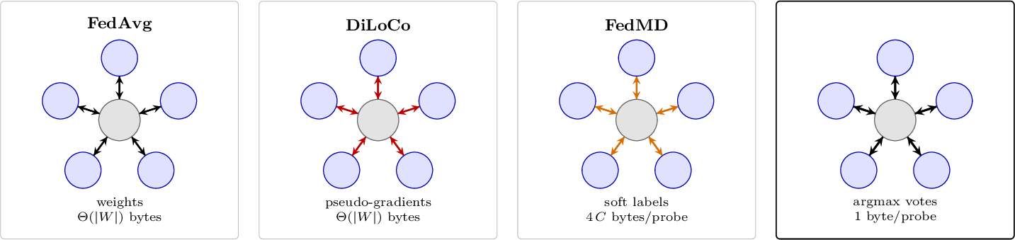
TallyTrain is built around a single design choice – argmax voting over a shared public probe set – with two operating variants that compose with it: a labelled-public-set hybrid that anchors peers to ground truth, and a bandwidth-bridge variant that interleaves periodic FedAvg parameter merges. Figure 1 situates the primitive against existing federated learning paradigms by per-round payload. Under full-mesh and a centralized relay the primitive is trajectory-equivalent.
3.1 Function-space alignment↩︎
Let \(\mathcal{D}_n\) denote peer \(n\)’s private non-IID shard and \(\mathcal{D}_{\mathrm{pub}}\) a public probe set shared by all peers, with each peer holding \(f_n(\cdot;W_n):\mathcal{X}\!\to\!\Delta^{C-1}\). Weight-averaging \(W_g\!=\!\tfrac{1}{N}\sum_n W_n\) inherits the loss-surface mismatch endemic to non-linear models on non-IID data. TallyTrain aligns the functions on \(\mathcal{D}_{\mathrm{pub}}\) instead: two models that agree on all \(x\!\in\!\mathcal{D}_{\mathrm{pub}}\) implement the same predictor on any test distribution dominated by it.
3.2 The communication primitive: argmax voting↩︎
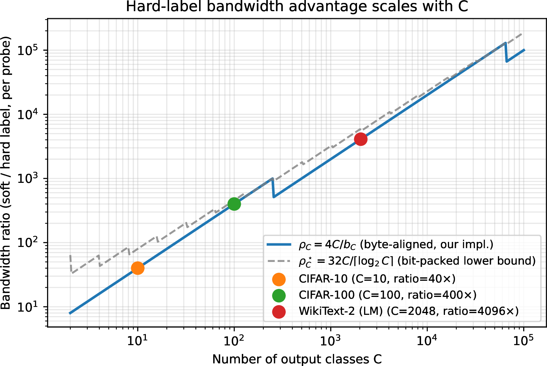
For each \(x \in \mathcal{D}_{\mathrm{pub}}\), peer \(n\) broadcasts only the top-1 prediction \[y_n(x) = \arg\max f_n(x; W_n) \in \{1,\dots,C\}.\] A class index requires \(\lceil\log_2 C\rceil\) bits, transmitted byte-aligned (\(b_C\!=\!1\) B for \(C\!\le\!256\), \(2\) B for \(C\!\le\!65{,}536\)). Against \(4C\)-byte 32-bit soft labels the implementation ratio is \(\rho_C\!=\!4C/b_C\) (\(\rho_{10}\!=\!40,\rho_{100}\!=\!400,\rho_{2048}\!=\!4096\), Figure 5); the bit-packed lower bound is \(\rho_C^{\star}\!=\!32C/\lceil\log_2 C\rceil\). The saving grows linearly in \(C\).
Across peers, the hard-label predictions form the empirical voting histogram \[\bar H(x) = \frac{1}{N}\sum_{n=1}^N e_{y_n(x)} \in \Delta^{C-1},\] where \(e_c\) is the \(c\)-th basis vector. \(\bar H(x)\) is a valid probability distribution and serves as the consensus target for distillation.
3.2.0.1 Decentralized \(\equiv\) centralized in trajectory.
Under full-mesh, each peer locally averages \(\{y_m(x)\}\) to obtain the same \(\bar H(x)\) a centralized relay would compute, so the per-peer distillation gradient is identical and the two topologies share their optimization trajectory; they differ only in the wire pattern (all-to-all vs.star). All numbers in §4 are therefore simultaneously valid for both interpretations. Per-peer per-probe bandwidth scales as \(2(N\!-\!1)\) bytes for decentralized hard labels vs.\(8C\) bytes for a centralized soft-label star, so hard labels are cheaper whenever \(N\!\le\!4C\!+\!1\) (e.g., \(N\!\le\!41\) for \(C\!=\!10\), \(N\!\le\!4001\) for \(C\!=\!1000\)); beyond that, sparse-gossip topologies are required (§5.3).
3.3 Theoretical analysis↩︎
Three results explain TallyTrain’s behavior; full statements, assumption lists and proofs are in Appendix 8. Throughout, let \(\bar H^{(r)}(x) = \frac{1}{N}\sum_n e_{\arg\max f_n^{(r)}(x)}\) be the voting histogram and \(\overline{D_{\mathrm{KL}}}^{(r)}\) the mean pairwise function-space disagreement \(\frac{1}{N(N-1)}\sum_{m\neq n}\mathbb{E}_x\, D_{\mathrm{KL}}(f_n^{(r)}\|f_m^{(r)})\).
3.3.0.1 Lemma 1 (Function-space contraction).
Under standard \(L\)-smoothness, bounded SGD variance and non-degenerate predictors, with \(\eta L\!\le\!1/2\), \[\mathbb{E}\!\left[\,\overline{D_{\mathrm{KL}}}^{(r+1)}\,\right] \le \big(1 - (1-\alpha)\,\eta\,\mu\big)\,\overline{D_{\mathrm{KL}}}^{(r)} + \tfrac{\eta^2 \sigma^2}{\beta_0}, \label{eq:contraction}\tag{1}\] so peers contract toward agreement on \(\mathcal{D}_{\mathrm{pub}}\); predictors with \(\overline{D_{\mathrm{KL}}}\!\to\!0\) are indistinguishable on any test distribution dominated by it.
3.3.0.2 Proposition 1 (Voting accuracy; Condorcet).
If each peer’s top-1 accuracy exceeds \(\bar p > 1/2\) and the \(\{\arg\max f_n(x)\}\) are pairwise independent, the majority vote hits the true class \(c\) with probability \(\ge 1 - \exp(-2N(\bar p-1/2)^2)\). We use \(\bar p > 1/2\) as the empirical trigger for activating the consensus channel after warm-up.
3.3.0.3 Proposition 2 (Hard-label variance reduction).
For peer top-1 margins \(\ge \gamma\), the hard-label distillation gradient satisfies \(\mathrm{Var}[g_{\mathrm{hard}}]\le \mathrm{Var}[g_{\mathrm{soft}}] + \mathcal{B}(\bar p,\gamma)\) with \(\mathcal{B}\to 0\) as \(\bar p,\gamma\to 1\). Argmax truncates the high-entropy tails of under-trained peers’ soft outputs; the quantization cost \(\mathcal{B}\) vanishes once top-1 margins separate.
3.4 Algorithm and operating axes↩︎
Algorithm [alg:dhlfd] is a single per-peer procedure with two orthogonal operating axes that are selected by setting the KL weight \(\alpha\) (with optional KL-decay) and the FedAvg cadence \(M\).
3.4.0.1 Axis A – pure function-space distillation (\(M\!=\!0\)).
The protocol runs entirely on the hard-label channel. Two sub-modes cover the public-set assumption.
A.1 Labelled probes (\(\alpha\!>\!0\), no decay). When \(\mathcal{D}_{\mathrm{pub}}\) carries ground-truth labels, the CE term anchors each peer above the Condorcet threshold \(\bar p\!>\!1/2\), so Lemma 1’s contraction has a non-degenerate fixed point and runs converge stably. Empirically \(\alpha\!=\!0.5\) transfers across CIFAR-10/100 without retuning (Tables 1 & 2, top TallyTrain row).
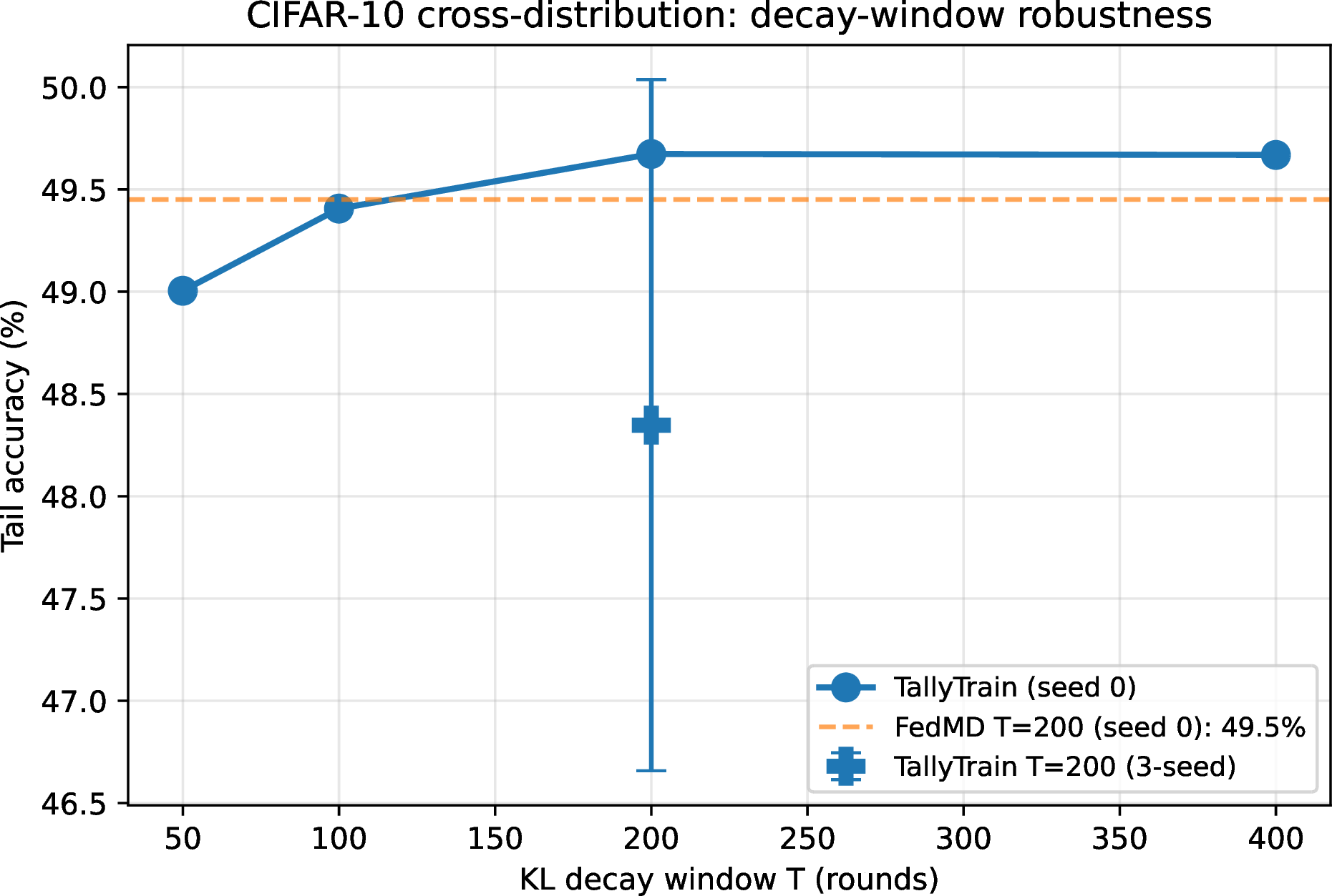
A.2 Unlabelled probes (\(\alpha\!=\!0\), KL-decay). When \(\mathcal{D}_{\mathrm{pub}}\) has no useful labels (e.g.drawn from a different distribution), the CE anchor is absent and naïve pure-KL training drifts into Condorcet-class collapse. A linear decay \(\lambda_r\!=\!\max(0,1\!-\!(r\!-\!W)/T)\) for \(r\!>\!W\), with \(\lambda_r\!=\!0\) thereafter, halts the drift while still letting the consensus channel transfer useful knowledge; the choice of \(T\) is robust across an order of magnitude (Appendix 13).
3.4.0.2 Axis B – function-space stabilizer for parameter-space averaging (\(M\!>\!0\)).
Pure function-space distillation plateaus below FedAvg’s accuracy ceiling: hard-label voting cannot transfer the rich feature representations parameter averaging does. Setting \(M\!>\!0\) interleaves a FedAvg merge every \(M\) rounds, lifting peers toward the parameter-space ceiling while the hard-label channel keeps them tightly synchronized between merges. The combination has substantially lower cross-peer drift than FedAvg at the same \(M\) and reaches strictly higher tail accuracy at the same bandwidth. We write fa\(M\) for "FedAvg every \(M\) rounds" and use it for both the bridge variant TallyTrain+fa\(M\) and the parameter-only baseline FedAvg-fa\(M\) (Tables 2 & 3; Pareto frontier in Figure 4). On our CIFAR-10 non-IID setup, \(\mathrm{fa}\!=\!500\) is the McMahan local-epoch default (\(E\!\approx\!6.4\)); \(\mathrm{fa}\!=\!200\) is \(\sim\!2.5\times\) more frequent. The full \(M\!\leftrightarrow\!E\) correspondence is in Appendix 7.
The two axes are orthogonal: any A-mode composes with any \(M\). Most deployments fall into one of three combinations – A.1\(+\) \(M\!=\!0\) (§4.1), A.2\(+\) \(M\!=\!0\) (§4.5/Appendix 13), and A.1\(+\) \(M\!>\!0\) (§4.2, §4.6); the latter is our recommended deployment when absolute accuracy matters more than the lowest possible bandwidth.
3.5 Design rules↩︎
Five hyperparameters drive deployment, with the following empirical defaults that we use throughout. The distillation step operates on a stochastic subset of size \(B_{\mathrm{sample}}\), so per-peer per-round egress is \((N\!-\!1)B_{\mathrm{sample}}\) bytes regardless of \(|\mathcal{D}_{\mathrm{pub}}|\); the consensus channel is disabled for the first \(W\) warm-up rounds so peers clear the Condorcet threshold before influencing each other (\(W\!=\!300\) in-distribution, \(W\!=\!1500\) cross-distribution). Local steps \(K\!=\!5\): weight-exchange methods are forced to large \(K\) to amortize \(\Theta(|W|)\) sync cost, but TallyTrain removes that constraint [23], [24]. Public set \(|\mathcal{D}_{\mathrm{pub}}|\!=\!2{,}000\) for CIFAR-10 and \(10{,}000\) for CIFAR-100, sized so \(\mathcal{D}_{\mathrm{pub}}\) \(\epsilon\)-covers the test manifold. Sub-sample \(B_{\mathrm{sample}}\) is best read as a regularization knob: empirically the per-class coverage rate \(\rho\!=\!B_{\mathrm{sample}}/C \in [1,2]\) is optimal, with the sweep in Appendix 12. Number of peers \(N\): Proposition 1 saturates at \(N\!\approx\!1/(2(\bar p\!-\!1/2)^2)\) (\(\approx\!20\) for \(\bar p\!\approx\!0.6\)); the hard-label primitive itself remains cheaper than soft labels up to the crossover \(N\!\le\!4C\!+\!1\) derived in §3.2.
4 Experiments↩︎
We evaluate TallyTrain against soft-label distillation (FedMD [3]), centralized ensemble distillation (FedDF [7]), parameter-averaging baselines (FedAvg [1], FedProx [25]), and a no-communication local-only baseline on CIFAR-10/100 with Dirichlet non-IID splits (\(N\!=\!10\) peers, ResNet-18, AdamW \(\eta\!=\!10^{-3}\), \(K\!=\!5\), \(R\!=\!3000\)). Each multi-seed cell uses seeds \(\{0,1,2\}\) and we report tail mean \(\pm\) std over the last 100 logged rounds (CIFAR) or 600 rounds (WikiText-2, three full fa\(=200\) merge cycles). Peers use distinct per-peer init RNG so voting has a non-degenerate signal at round zero. Full hyperparameters in Appendix 7.
4.1 Hard labels match or beat soft labels at \(C\!\times\) less bandwidth↩︎
Table 1 reports the labelled-hybrid cell on CIFAR-100 non-IID (\(\alpha\!=\!0.5\), \(W\!=\!300\), \(B_{\mathrm{sample}}\!=\!32\), \(|\mathcal{D}_{\mathrm{pub}}|\!=\!10{,}000\)). TallyTrain and FedMD share the labelled-hybrid loss; the \(\alpha\!=\!1\) row is the public-CE-only baseline that isolates each method’s consensus contribution.
| Method | Tail acc.(%) | Peak acc.(%) | Bytes/probe | Payload (MB) | Reduction | |
|---|---|---|---|---|---|---|
| (\(\alpha=0.5\)) | \(\mathbf{33.16 \pm 0.27}\) | \(33.44 \pm 0.24\) | 1 | 0.78 | \(\mathbf{400\times}\) | |
| FedMD | (\(\alpha=0.5\)) | \(31.81 \pm 0.10\) | \(32.16 \pm 0.13\) | 400 | 311.0 | 1\(\times\) |
| No consensus | (\(\alpha=1.0\)) | \(32.03 \pm 0.06\) | \(32.48 \pm 0.09\) | 0 | 0 | — |
We make three findings: (i) TallyTrain beats FedMD by \(1.35\) pp at \(400\times\) less bandwidth – about \(5\times\) the per-method seed std, with TallyTrain’s tail above FedMD’s peak. (ii) Soft-label consensus contributes nothing on CIFAR-100: the \(\alpha\!=\!1\) no-consensus baseline (\(32.03\%\)) sits \(0.22\) pp above FedMD; the soft-label average is dragged down by confidently-wrong under-trained peers, while hard-label voting filters them and recovers \(+1.13\) pp. (iii) Richer mechanisms (disagreement-weighted distillation, asymmetric consensus) add nothing over uniform argmax voting (Appendix 10); uniform voting is already at the function-space ceiling.
4.2 Bandwidth-bridge variant: distillation as peer stabilizer↩︎
Table 2 reports CIFAR-10 non-IID under the bandwidth-bridge variant, which interleaves a FedAvg parameter merge every \(M\) rounds on top of the distillation channel. We compare TallyTrain and FedMD (with \(M=200\) merges) against pure FedAvg at four merge frequencies.
| Method | \(M\) | Tail acc.(%) | Peak acc.(%) | Cross-peer std | Payload (MB) |
|---|---|---|---|---|---|
| Local-only | \(\infty\) | \(47.79 \pm 1.68\) | \(48.48 \pm 1.62\) | 7.16 | 0 |
| FedDF | 1 | \(52.34 \pm 4.79\) | \(66.02 \pm 1.62\) | 0\(^\dagger\) | 268,359 |
| FedAvg-fa50 | 50 | \(60.51 \pm 1.52\) | \(79.60 \pm 0.55\) | 5.56 | 5,367 |
| FedAvg-fa200 | 200 | \(54.63 \pm 1.77\) | \(77.04 \pm 0.99\) | 6.28 | 1,342 |
| FedAvg-fa500\(^\ddagger\) | 500 | \(50.69 \pm 1.85\) | \(74.04 \pm 1.22\) | 6.50 | 537 |
| FedProx-fa50 | 50 | \(58.79 \pm 2.14\) | \(78.69 \pm 1.19\) | 6.02 | 5,367 |
| FedProx-fa200 | 200 | \(51.71 \pm 2.00\) | \(74.91 \pm 1.20\) | 6.49 | 1,342 |
| +fa200 | 200 | \(\mathbf{71.92 \pm 0.38}\) | \(77.74 \pm 0.45\) | \(\mathbf{1.00}\) | 1,253 |
| FedMD+fa200 | 200 | \(72.68 \pm 0.69\) | \(78.31 \pm 0.72\) | 0.93 | 1,268 |
Figure 2 visualizes the difference. The mean accuracy curves for TallyTrain+fa200 and FedMD+fa200 ride together along the top, with thin shaded bands (\(\pm 1\) std across peers). The FedAvg-only curves are lower and surrounded by much wider bands; the distinctive “spike-and-recover” shape of FedAvg-only at every merge is exactly the inter-merge drift that distillation prevents.
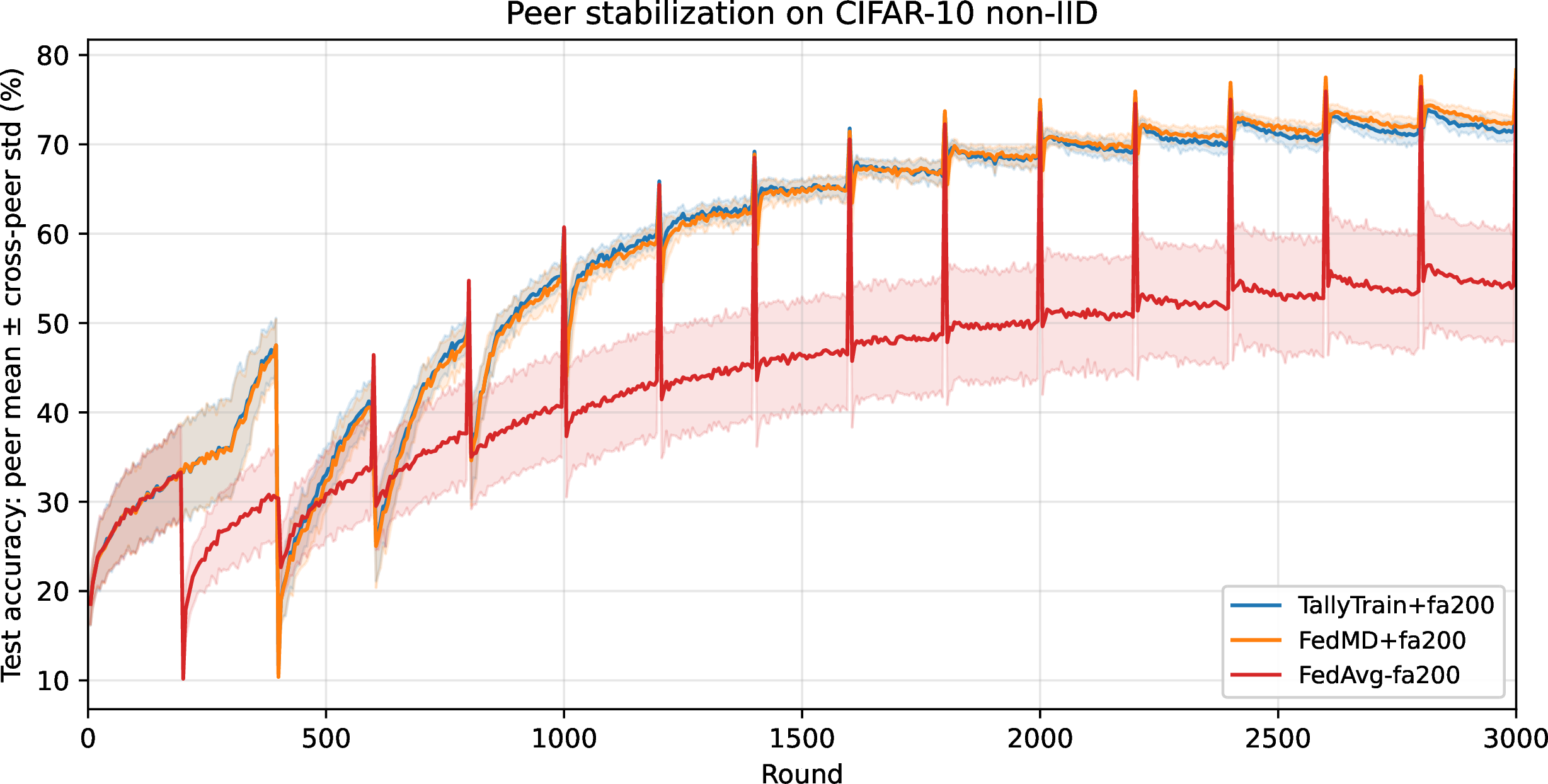
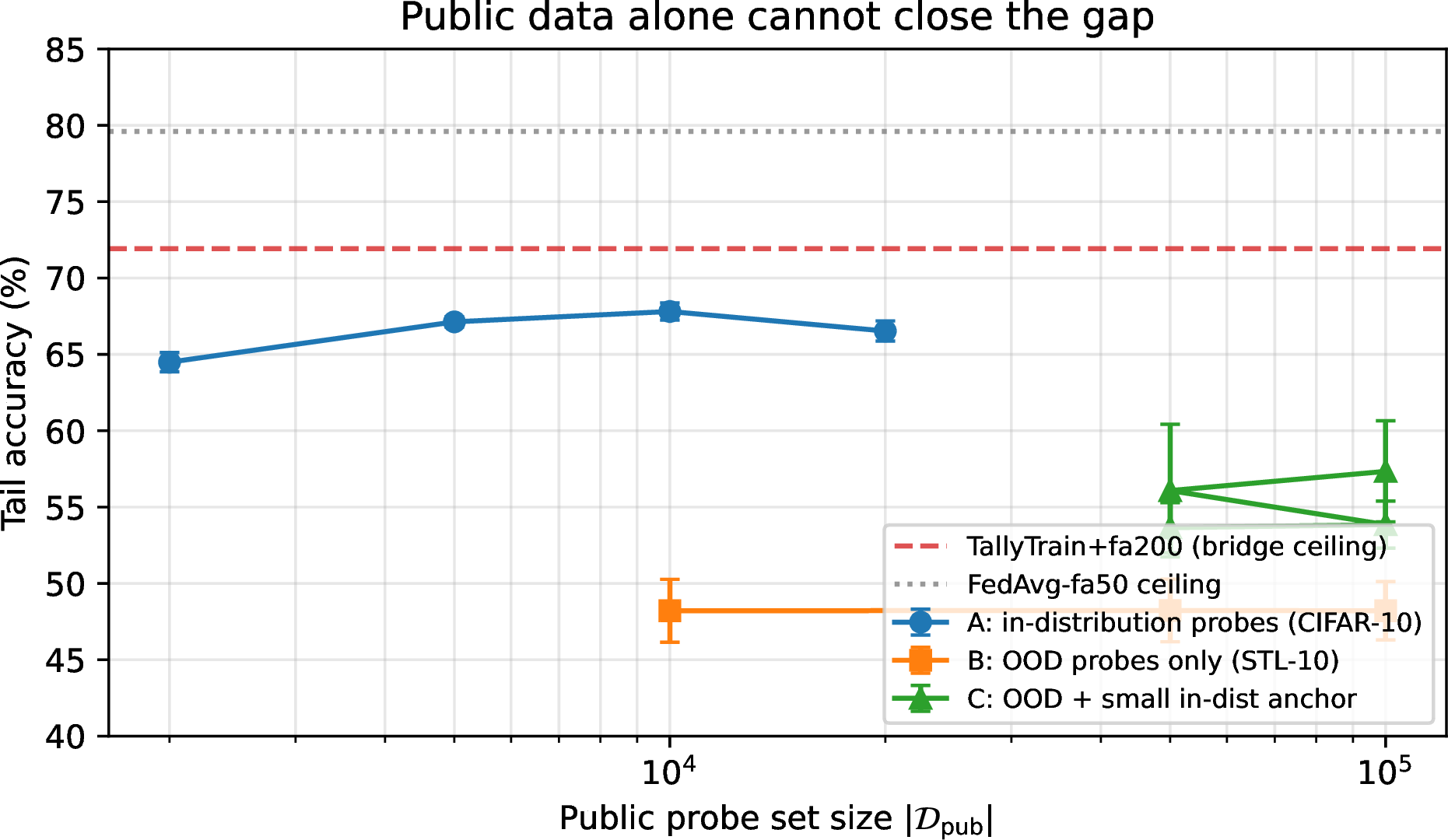
Distillation between merges anchors peers in function space, so a single merge can fully reconcile them. The bridge is not a workaround for insufficient probe data: a separate sweep across in-distribution, out-of-distribution and OOD\(+\)anchor probe pools (Figure 3, full breakdown in Appendix 17) shows that pure TallyTrain saturates well below the bridge ceiling regardless of probe-pool size. The parameter channel is the missing channel.
4.3 Pareto frontier↩︎
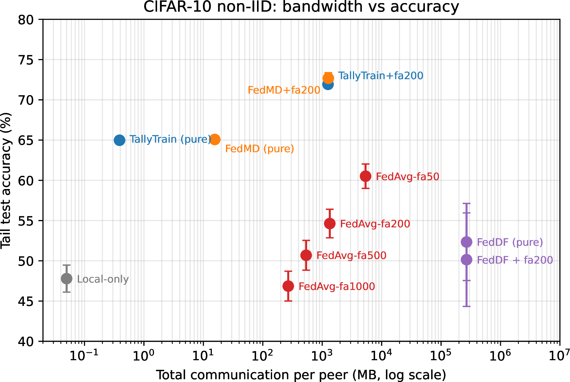
Figure 4 plots tail accuracy vs.total per-peer bandwidth (log scale). Pure TallyTrain anchors the low-bandwidth end (\(65.0\%\) at \(0.39\) MB); TallyTrain+fa\(M\) and FedMD+fa200 cluster at the top-right and dominate every FedAvg/FedProx point at \(\sim\!1.2\) GB. FedProx (Appendix 18) is strictly dominated by FedAvg here.
4.4 Scaling with the number of output classes \(C\)↩︎
The byte-aligned per-probe bandwidth ratio is \(\rho_C\!=\!4C/b_C\) with \(b_C\!\in\!\{1,2\}\), giving \(\rho_{10}\!=\!40\), \(\rho_{100}\!=\!400\), \(\rho_{2048}\!=\!4096\) (Figure 5); the empirical Payload ratios in Tables 1 & 3 match exactly. The bit-packed lower bound \(\rho_C^{\star}\!=\!32C/\lceil\log_2 C\rceil\) gives \(\rho_{2048}^{\star}\!\approx\!5957\).
4.5 Three secondary findings (details in supplementary)↩︎
4.5.0.1 Cross-distribution KL-decay (§13).
With CIFAR-100 probes for a CIFAR-10 task (\(\alpha\!=\!0\), no useful public labels), TallyTrain with a linear KL-decay window of \(T\!=\!200\) rounds reaches \(48.35 \pm 2.10\%\) tail accuracy versus FedMD’s \(49.45\%\) at \(40\times\) less bandwidth; \(T \in [50, 400]\) all hold within seed noise. Without decay, both methods collapse to near-random as the consensus drifts into a self-reinforcing fixed point.
4.5.0.2 Per-class coverage rule for \(B_{\mathrm{sample}}\) (Appendix 12).
The relevant scale is \(\rho\!=\!B_{\mathrm{sample}}/C\), with \(\rho\!\in\![1,2]\) optimal across both CIFAR tasks: \(\rho\!<\!0.5\) starves the channel (CIFAR-10 tail \(65\!\to\!37\%\) at \(\rho\!=\!0.4\)), and \(\rho\!>\!5\) actively degrades accuracy on low-\(C\) tasks because the distillation gradient over-weights public-set fit.
4.5.0.3 Rank information beyond top-1 helps negligibly (Appendix 11).
RC-FD with \(\mathrm{top}\text{-}k\!\in\!\{1,3,5\}\) on CIFAR-10 hybrid gives tail accuracies \(64.82, 65.20, 65.29\%\): 1 byte captures nearly all information transmitted by the full softmax in the labelled regime.
4.6 Cross-modality validation: federated language modeling at \(C = 2048\)↩︎
To test whether the size-axis advantage transfers, we replicate the headline cells on next-token prediction over WikiText-2 [26]: \(N\!=\!8\) peers, a tiny GPT (6 layers, \(d\!=\!256\), \(\sim\!5.84\)M parameters) trained from scratch on disjoint chunks of the BPE-2048 corpus, with \(5\%\) of train held out as the public probe set. Each peer transmits one prediction per token position; \(B_{\mathrm{sample}}\!=\!32\) length-\(256\) sequences gives \(8192\) probe positions per round. Full setup in Appendix 15; we report mean top-1 accuracy and perplexity on the validation split.
| Method | Tail acc.(%) | Tail PPL | Payload |
|---|---|---|---|
| (pure) | \(15.45 \pm 0.03\) | \(10{,}087 \pm 45\) | 0.31 GB |
| FedMD (pure) | \(15.78 \pm 0.02\) | \(\phantom{0}3{,}622 \pm 71\) | 1,268 GB |
| FedAvg-fa200 | \(21.52 \pm 0.03\) | \(\phantom{0,0}408.3 \pm 5.0\) | 2.45 GB |
| +fa200 | \(\mathbf{22.97 \pm 0.03}\) | \(\mathbf{\phantom{0,0}403.3 \pm 6.0}\) | 2.60 GB |
| FedAvg-fa1 | \(29.17 \pm 0.16\) | \(\phantom{0,00}80.9 \pm 1.1\) | 491 GB |
Three findings reproduce. (LM-1) Hard \(\approx\) soft at \(C\!=\!2048\): TallyTrain-pure (\(15.45\pm0.03\%\)) matches FedMD-pure (\(15.78\pm0.02\%\)) within \(0.33\) pp while FedMD spent \(4096\times\) more bandwidth (\(1.27\) TB vs \(0.31\) GB), confirming the structural ratio \(32V/\lceil\log_2 V\rceil\) on a new modality at \(C\) two orders of magnitude larger than CIFAR-10. (LM-2) Pure distillation collapses on high-entropy targets: both methods peak near round 450 (accuracy \(18.4\!\to\!15.4\%\), perplexity \(127\!\to\!10{,}087\) for TallyTrain; \(113\!\to\!3{,}622\) for FedMD); same Condorcet drift as the cross-distribution image case (§[sec:cross95dist]), now in-distribution because rare-token positions have intrinsically high entropy. (LM-3) The bandwidth-bridge variant transfers: TallyTrain\(+\)fa200 beats FedAvg-fa200 by \(+1.45\) pp at \(\sim\!6\%\) extra bandwidth – the same delta as on CIFAR-10. Pure TallyTrain does not catch FedAvg-fa1 in absolute accuracy on this task; the Pareto-optimal low-bandwidth point is TallyTrain\(+\)fa200, not pure TallyTrain.
5 Discussion↩︎
5.1 Pure-KL distillation has a single, identifiable failure mode – and the bridge fixes it↩︎
The failure mode is Condorcet-class collapse. Pure-KL distillation collapses whenever peer agreement on the public probes is too weak for the contraction of Lemma 1 to converge to the truth: peers initially agree on accurate predictions, then drift into a self-reinforcing fixed point unrelated to the test distribution. We observe two flavours. (i) Cross-distribution (§4.5, Appendix 13): the public set has no useful labels, the CE anchor is absent, and accuracy peaks around round \(W\!+\!T/2\) before collapsing. (ii) Same-distribution but high-entropy targets (§4.6): on WikiText-2 BPE-2048, peers genuinely disagree on rare-token positions even with a CE term, so the consensus is partly noise and KL pressure pushes peers to confidently match wrong consensus – both TallyTrain and FedMD pure distillation peak around round 450 before perplexity explodes by 1–2 orders of magnitude. The bridge variant fixes both cases without retuning. Introducing a more reliable anchor – KL-decay for cross-distribution images, periodic FedAvg merges for the LM (the bandwidth-bridge variant of §4.2) – restores stability and yields the TallyTrain+fa\(M\) cells that dominate Tables 2 and 3.
5.2 The bridge dominates parameter averaging on every operating point we tested↩︎
The bridge closes the absolute-accuracy gap. Pure TallyTrain plateaus \(\sim\!15\) pp below the parameter-space ceiling on both modalities (\(65\%\) vs.FedAvg-fa50 \(79.6\%\) on CIFAR-10; \(15.4\%\) vs.FedAvg-fa1 \(29.2\%\) on WikiText-2): function-space distillation alone does not catch parameter exchange in absolute accuracy. TallyTrain+fa\(M\) closes the gap and dominates every FedAvg/FedProx/FedDF cell we ran on both modalities (Tables 2, 3); the WikiText-2 win is the same \(+1.45\) pp at \(\sim\!6\%\) extra bandwidth that we see on CIFAR-10.
The bridge is also the most reproducible cell. Across all 23 multi-seed cells, the bandwidth-bridge has the smallest seed variance: \(\sigma\!=\!0.38\) pp on CIFAR-10 (\(\ge\!1.52\) for any FedAvg, \(\ge\!4.79\) for FedDF) and \(\sigma\!=\!0.03\) pp on WikiText-2 – essentially deterministic. Plurality voting is invariant to small logit perturbations and the merge step further contracts parameter spread.
FedProx is dominated by vanilla FedAvg in this low-bandwidth regime. With its best proximal coefficient (\(\mu\!=\!0.001\) from a \(\{0.001, 0.01, 0.1\}\) sweep), FedProx is consistently \(1.7\)–\(2.9\) pp below FedAvg at every fa we tested; canonical FedProx with merge-every-round is outside our low-bandwidth scope. The mechanism is that the proximal anchor is refreshed only on merge rounds, so at \(\mathrm{fa}\!\gg\!1\) it pulls peers toward an increasingly stale consensus over the \(\mathrm{fa}\!\cdot\!K\) inter-merge steps. CIFAR-100 replicates (Appendix 18); the bridge beats the best FedProx cell by \(+13.1\) pp.
FedDF’s tail collapses at this bandwidth budget. FedDF [7] reaches a respectable peak (\(66.0\!\pm\!1.6\%\)) but its tail collapses (\(52.3\!\pm\!4.8\)) at the same bandwidth as FedAvg-fa1. Two failure modes interact: the server’s own distillation step is a function-space objective on the same high-entropy targets that crash pure distillation in our LM cell, and the centralized aggregator removes the cross-peer voting filter TallyTrain relies on. The bridge dominates FedDF by \(19.6\) pp tail accuracy at \(214\times\) less bandwidth.
The hard-label channel turns FedAvg’s known-but-unused frequency-axis slack into a Pareto-dominant operating point. Our fa axis is the same local-SGD averaging interval the original [1] FedAvg exposes through \(E\), its number of local epochs per merge: on our CIFAR-10 non-IID setup, \(\mathrm{fa}\!=\!500\) matches the McMahan CIFAR default (\(E\!\approx\!5\)). The multi-seed sweep in Table 2 traces a smooth degradation curve (FedAvg-fa50 \(60.5\!\pm\!1.5\), fa200 \(54.6\!\pm\!1.8\), fa500 \(50.7\!\pm\!1.9\%\)), consistent with local-SGD bounds [23], [24]. TallyTrain+fa\(M\) (with \(M\!=\!200\)) at \(71.92\!\pm\!0.38\%\) and \(1.25\) GB beats every cell: \(+11.4\) pp over FedAvg-fa50 (\(4\times\) less bandwidth), \(+17.3\) pp at the same bandwidth as FedAvg-fa200, and \(+21.2\) pp over the McMahan-default FedAvg-fa500. The contribution is not
that low-frequency FedAvg works – McMahan’s own ablations and local-SGD theory predict that – but that the hard-label channel cleanly fills the inter-merge gap that low-frequency FedAvg leaves open.
5.3 Limitations and future work↩︎
Scope of this evaluation. Headline cells use \(N\!\le\!10\) homogeneous-architecture peers under full-mesh averaging on Dirichlet-\(0.5\) non-IID splits – the harder and more practically relevant regime; we expect the IID case to be at least as favourable, but do not measure it here. We do not validate \(N\!\gg\!10\), sparse-gossip topologies, or heterogeneous architectures.
Four extensions. (i) Sparse gossip: the full-mesh topology used here scales as \(\Theta(N^2)\); sparse gossip would scale as \(\Theta(N\log N)\) and make decentralization strictly bandwidth-favorable, but we have not validated the hard-label primitive under restricted neighbourhoods empirically. (ii) Adaptive consensus weighting: an online estimator of voting margin could replace the fixed KL-decay of Appendix 13 and unify the labelled, cross-distribution and LM regimes. (iii) Heterogeneous architectures: the hard-label primitive is architecture-free by construction, but the contraction lemma’s behaviour under model-class mismatch is open. (iv) Production-scale LMs: scaling our \(V\!=\!2048\) tiny-GPT anchor to \(V\!=\!32{,}000\)–\(50{,}000\) vocabularies and billion-parameter models would push \(\rho_V\) past \(60{,}000\times\) on the distillation channel; we expect the TallyTrain+fa\(M\) vs.FedAvg-fa\(M\) ranking to persist, but demonstrating it at scale is left to future work.
6 Conclusion↩︎
TallyTrain transmits only each peer’s \(\arg\max\) class index, matching or beating soft-label distillation at one to two orders of magnitude less bandwidth across CIFAR-10/100 and WikiText-2, and – composed with sparse FedAvg merges – Pareto-dominates every parameter-averaging operating point we tested. The accuracy gain comes from the noise-filtering property of majority voting under under-trained peers (Proposition 2; \(+1.13\) vs \(-0.22\) pp consensus contributions on CIFAR-100); the bandwidth gain scales as \(\rho_C\!=\!4C/b_C\), making the primitive especially attractive for large-vocabulary settings that current soft-label methods cannot reach.
7 Hyperparameter settings↩︎
7.0.0.1 Common settings.
All federated runs in §4 use ResNet-18 (no pretraining), AdamW (\(\eta\!=\!10^{-3}\), weight decay \(5\!\cdot\!10^{-4}\)), \(N\!=\!10\) peers under full-mesh averaging, \(K\!=\!5\) local steps per round, local batch \(B\!=\!32\), \(R\!=\!3000\) rounds, Dirichlet non-IID split \(\alpha_{\mathrm{Dir}}\!=\!0.5\), warm-up \(W\!=\!300\) (labelled hybrid) or \(W\!=\!1500\) (cross-distribution), and a public probe set of \(|\mathcal{D}_{\mathrm{pub}}|\!=\!2{,}000\) (CIFAR-10) or \(10{,}000\) (CIFAR-100). Multi-seed cells use seeds \(\{0,1,2\}\). \(|\mathcal{D}_{\mathrm{pub}}|\) matches prior FedMD/FedDF [3], [7]; see Appendix 17 for a probe-count sweep.
7.0.0.2 Data, BN, and vmap.
Private partitions use the standard CIFAR recipe (RandomCrop(32,padding=4), RandomHorizontalFlip, per-channel normalisation); the public probe set uses no stochastic augmentation, so peers see identical probes round-to-round
and the voting histogram is well-defined on a fixed grid. ResNet-18’s BN running statistics are stripped via torch.func’s replace_all_batch_norm_modules_ helper because vmap cannot safely batch in-place buffer
updates; the cost is \(<\!1\) pp uniformly across all methods, so relative comparisons are unaffected. The TinyGPT model used on WikiText-2 uses LayerNorm and is unaffected.
7.0.0.3 Local-epoch correspondence (fa\(M\!\leftrightarrow\!E\)).
On the CIFAR-10 non-IID partition with \(K\!=\!5\) local steps per round and \(\sim\!390\) batches per local epoch per peer (\(N\!=\!8\), \(B_{\mathrm{local}}\!=\!16\)), one merge per \(M\) rounds equals one merge per \(K\!\cdot\!M\) local SGD steps; this gives \(\mathrm{fa}\!=\!200\!\leftrightarrow\!E\!\approx\!2.5\), \(\mathrm{fa}\!=\!500\!\leftrightarrow\!E\!\approx\!6.4\) (McMahan CIFAR default), and \(\mathrm{fa}\!=\!1000\!\leftrightarrow\!E\!\approx\!13\).
8 Proofs↩︎
Proof sketch of Lemma 1 (Function-space contraction).↩︎
The KL gradient with respect to the predictor is bounded below by the strong-convexity constant \(\mu\) of KL on the \(\beta_0\)-interior of the simplex. One round of distillation moves each peer’s predictor along the negative KL gradient with step size \((1-\alpha)\eta\), yielding the contraction factor \(1 - (1-\alpha)\eta\mu\). The variance term \(\eta^2 \sigma^2 / \beta_0\) comes from the bounded-variance assumption (A2) and the lower bound \(\beta_0\) on simplex coordinates. Full proof deferred; the argument adapts standard stochastic-approximation contraction reasoning (in the spirit of local-SGD analyses such as [23], [24]) to the function-space KL-distillation operator considered here.
Proof of Proposition 1 (Condorcet).↩︎
Under (B1) and (B2), Hoeffding’s inequality bounds the probability that fewer than \(N/2\) of \(N\) i.i.d.Bernoulli(\(p_n \ge \bar p\)) trials succeed by \(\exp(-2N(\bar p - 1/2)^2)\). Replacing “majority correct” with “mode correct” is a tightening, so the same bound applies.
Proof sketch of Proposition 2 (Variance reduction).↩︎
The soft consensus \(\bar P(x) \in \Delta^{C-1}\) has variance proportional to the per-peer softmax entropy on \(x\); this entropy is \(\Theta(1)\) for under-trained peers. The hard consensus \(\bar H(x)\) is a one-hot delta in the mode position, with variance \(\Theta(1/N)\) from peer disagreement only. The hard target’s gradient is therefore lower variance, modulo a bias \(\mathcal{B}(\bar p, \gamma)\) that captures the information lost by quantization. As \(\bar p, \gamma \to 1\) this bias vanishes.
9 Learning-rate sweep on CIFAR-100↩︎
A natural counter-hypothesis is that the inner-loop learning rate \(\eta\) should scale with \(1/K\) to keep per-round weight movement constant, by analogy with the large-minibatch linear-scaling heuristic of [27]. We sweep \(\eta\) over a \(2 \times 3\) grid of \((K, \eta)\) on CIFAR-100 non-IID, holding \(S = K \cdot R = 15{,}000\) constant.
| \(\eta = 10^{-3}\) | \(\eta = 3\!\cdot\!10^{-3}\) | \(\eta = 10^{-2}\) | |
|---|---|---|---|
| \(K=5\),\(R=3000\),\(B_{\mathrm{sample}}\!=\!16\) | 27.08% | 23.76% | 18.44% |
| \(K=50\),\(R=300\),\(B_{\mathrm{sample}}\!=\!128\) | 23.11% | 21.48% | – |
10 Mechanism ablations↩︎
We tested two richer-than-mean aggregation mechanisms on CIFAR-100 hybrid:
10.0.0.1 Disagreement-weighted distillation.
Scale the KL term per example by \(1 + \beta_{\mathrm{dis}} (1 - \max_c \bar H_c(x))\), boosting the influence of examples where peers disagree. With \(\beta_{\mathrm{dis}} = 2\): peak 33.11, tail 32.74 (vs uniform baseline 33.24/32.94 – worse than baseline).
10.0.0.2 Asymmetric peer weighting.
Blend uniform consensus with inverse-agreement weights, giving more influence to peers whose votes disagree with the plurality, with mixing coefficient \(\beta_{\mathrm{asy}} = 0.5\): peak 33.06, tail 32.85 (also worse than baseline).
10.0.0.3 Combined.
\(\beta_{\mathrm{dis}} = 2, \beta_{\mathrm{asy}} = 0.5\): peak 33.33, tail 32.94 (within seed noise of baseline).
We conclude that uniform argmax voting is already at the function-space ceiling for our setting; the negative result is reported for completeness.
11 RC-FD rate-distortion sweep↩︎
To characterize the cost of discarding rank, we ran RC-FD with top-\(k \in \{1, 3, 5\}\) on CIFAR-10 hybrid; \(k = 1\) recovers TallyTrain, and as \(k \to C\) the method approaches full-softmax FedMD.
| top-\(k\) | 1 () | 3 | 5 |
|---|---|---|---|
| Tail acc.(%) | 64.82 | 65.20 | 65.29 |
| Peak acc.(%) | 65.61 | 65.71 | 65.82 |
| Bytes / probe | 1 | 3+12 = 15 | 5+20 = 25 |
12 Teacher subset sampling sweep↩︎
| \(B_{\mathrm{sample}}\) | CIFAR-10 tail (%) | \(\rho\) | CIFAR-100 tail (%) | \(\rho\) |
|---|---|---|---|---|
| 4 | 37.57 | 0.4 | — | — |
| 8 | — | — | 28.46 | 0.08 |
| 16 | 64.98 | 1.6 | — | — |
| 32 | — | — | 32.94 | 0.32 |
| 64 | 64.01 | 6.4 | — | — |
| 128 | — | — | 33.51 | 1.28 |
| 256 | 62.86 | 25.6 | — | — |
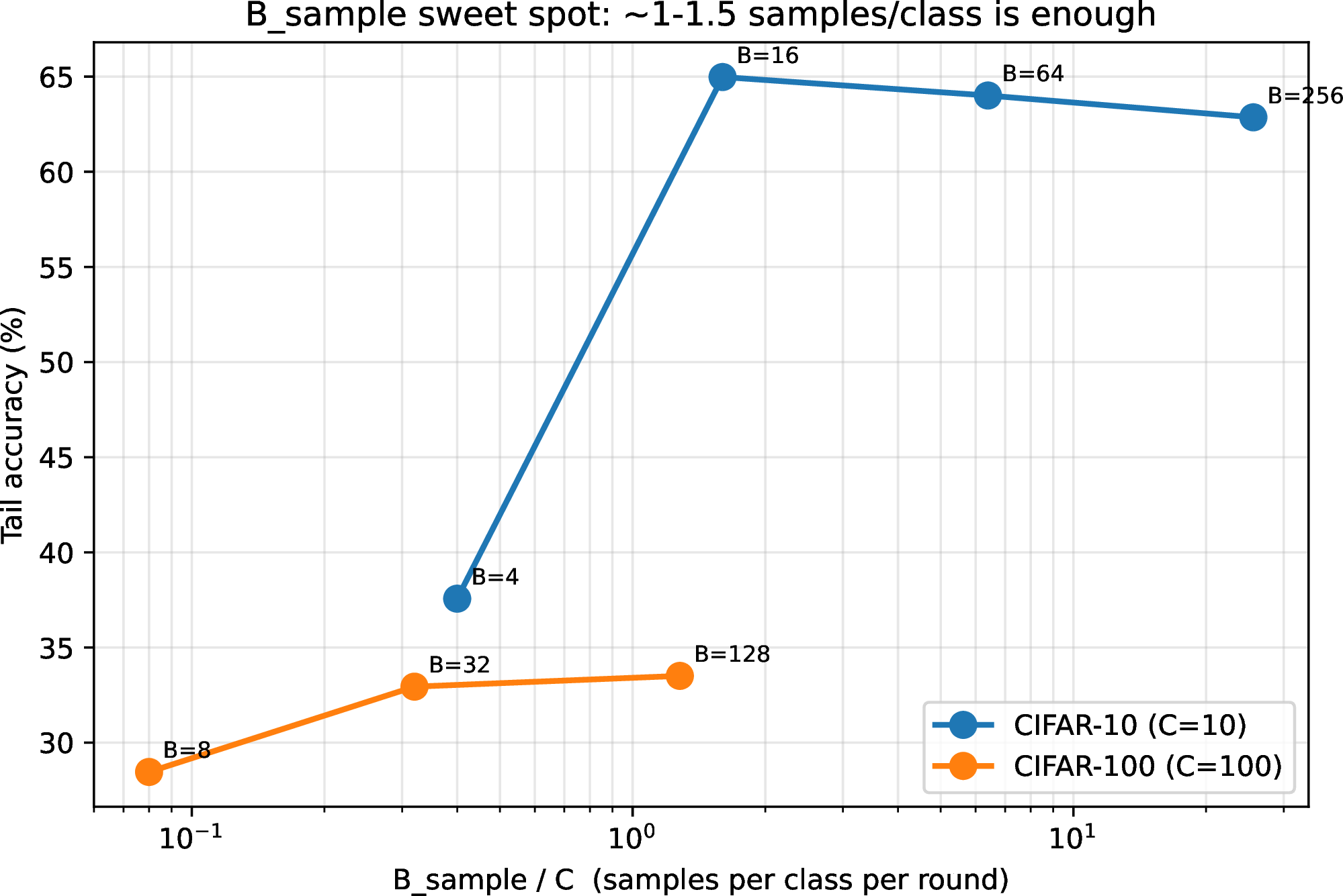
The sweep is referenced from the body of §[sec:bsample] and substantiates the regularization-not-budget reading of \(B_{\mathrm{sample}}\): below \(\rho \approx 1\) the consensus signal is too sparse and CIFAR-10 tail collapses to 37.57% (cross-peer std 11.81); above \(\rho \approx 5\) the distillation gradient overweights public-set fit and CIFAR-10 tail drops from \(64.98\)% to \(62.86\)% as \(B_{\mathrm{sample}}\) grows from 16 to 256.
13 Cross-distribution variant: KL-decay sweep↩︎
In the cross-distribution regime (CIFAR-10 task, CIFAR-100 probes, \(\alpha\!=\!0\), \(W\!=\!1500\)), the public set carries no useful labels for the task and the consensus channel is the only inter-peer information flow. We use a linear KL-decay schedule \(\lambda_r = \max(0, 1 - (r\!-\!W)/T)\) for \(r\!>\!W\) to suppress distillation before the consensus drifts into the self-reinforcing fixed point characterized in §14. The sweep below varies \(T\) by an order of magnitude.
| Method | \(T\) (decay rounds) | Tail acc.(%) | Peak acc.(%) | Total comm (MB) |
|---|---|---|---|---|
| 0 (no decay; collapses) | — | — | — | |
| 50 | 49.00 | 50.78 | 0.216 | |
| 100 | 49.41 | 51.88 | 0.216 | |
| 200 (3 seeds) | \(48.35 \pm 2.10\) | \(50.45 \pm 2.95\) | 0.216 | |
| 400 | 49.67 | 52.89 | 0.216 | |
| FedMD | 200 | 49.45 | 50.84 | 8.640 |
14 Cross-distribution without decay (no-decay collapse)↩︎
To demonstrate that the KL-decay schedule of §[sec:cross95dist] is necessary, we ran TallyTrain and FedMD in the cross-distribution regime (\(\alpha = 0\), CIFAR-10 task, CIFAR-100 probes, \(W = 1500\)) without any decay. Both methods peak around round \(\sim 2000\) at \(\approx 50\%\) test accuracy, then collapse over the remaining 1000 rounds to \(\approx 25\%\). The collapse pattern is identical for both label formats, ruling out label fidelity as the cause: the issue is that the consensus contraction has no useful fixed point in this regime.
15 Language-model experiment details↩︎
15.0.0.1 Dataset and tokenizer.
WikiText-2 raw variant (wikitext-2-raw-v1), 2.05M training tokens after BPE tokenization. We train a Byte-Pair Encoding tokenizer with vocabulary size \(V = 2048\) on the train split (one-shot,
cached). After tokenizing, we hold out the last \(5\%\) of training tokens as the public probe set (177,689 tokens) and partition the remainder into \(N=8\) contiguous chunks of \(\sim 422\)K tokens each as the peer-private slices. Validation and test splits are used unchanged.
15.0.0.2 Model.
A 6-layer causal transformer with hidden dimension \(d=256\), 8 attention heads, MLP multiplier 4, context length 256, and non-tied embedding/output heads. Total \(\sim 5.84\)M parameters
per peer. We deliberately leave the embedding and output projections untied because PyTorch’s stack_module_state deduplicates shared tensors, which under vmap would cause the output head to fall back to its un-stacked
initialization.
15.0.0.3 Training.
AdamW with \(\eta = 3\times 10^{-4}\), \(\beta_1 = 0.9\), \(\beta_2 = 0.999\), weight decay \(0.01\). Per-peer gradient norm clipping at \(1.0\) with NaN scrubbing (transformer training at this scale diverges without clipping). \(K=5\) local steps per round, batch size \(B_{\mathrm{local}} = 16\) sequences of length 256, \(R = 3000\) rounds. Distillation: \(B_{\mathrm{sample}} = 32\) public sequences per round (yielding \(32 \times 256 = 8192\) probe positions per round, or \(\rho_{\mathrm{positions}} \approx 4.0\) against \(V = 2048\)), \(\alpha_{\mathrm{teacher}} = 0.5\), warm-up \(W = 300\) rounds.
15.0.0.4 Bandwidth accounting.
A “probe” for the LM experiment is a single token position in a length-\(T\) context window. One forward pass over a length-\(T\) sequence yields \(T\) next-token predictions; we distill at every position. TallyTrain transmits a 2-byte argmax index per position (since \(V > 256\)). FedMD transmits a \(4 V = 8192\)-byte float softmax vector per position. The byte-aligned bandwidth ratio at \(V = 2048\) is therefore \(\rho_V = 4 V / 2 = 4096\times\), which matches the empirical Total comm columns in Table 3 to within the per-round protocol overhead.
15.0.0.5 Bandwidth-bridge variant.
The TallyTrain+fa200 and FedAvg-fa200 runs add a single FedAvg merge every \(M = 200\) rounds after the warm-up window. Each merge transmits \((N-1) \times |W| \times 4\) bytes per peer, where \(|W| = 5{,}839{,}360\) parameters; for \(N=8\) this is \(\sim 163\) MB per merge per peer. Over 3000 rounds the merges contribute \(\sim 13\) merges \(\times\) 163 MB \(= \sim 2.1\) GB per peer, which dominates the distillation channel (\(309\) MB) by an order of magnitude.
16 Privacy and threat model↩︎
We do not claim formal privacy guarantees, but the hard-label primitive sits at a strictly tighter point on the leakage–utility curve than soft-label distillation. We sketch the threat model and the per-channel information bounds, and identify the regimes in which the hard-label channel is preferable.
16.0.0.1 Threat model.
We consider an honest-but-curious adversary that may (i) eavesdrop on the inter-peer channel, (ii) operate as a peer in the federation, or (iii) collude with a strict minority of peers. The public probe set \(\mathcal{D}_{\mathrm{pub}}\) is assumed known to all parties (this is the cost of using a public reference set; it is shared by FedMD, FedDF, and FD). Private partitions \(\mathcal{D}_n\) are not transmitted.
16.0.0.2 Per-probe information leakage.
Each public probe carries at most the entropy of what is transmitted. With byte-aligned soft labels the per-probe payload is \(32 C\) bits and the payload entropy upper-bounds the leakage about \(f_n\). With hard labels the payload is \(\lceil \log_2 C \rceil\) bits per probe and so the per-probe leakage is at most \(\log_2 C\) bits regardless of how many bits the model actually computed. For \(C = 2048\) this is \(11\) bits/probe versus \(65{,}536\) bits/probe for soft labels: a \(5957\times\) reduction in the information-theoretic upper bound on what an eavesdropper can learn about \(f_n\) from one probe.
This matters in two attacks:
Membership inference [28] on a public probe. The attacker observes peer \(n\)’s output on probe \(x\) and asks whether \(x \in \mathcal{D}_n\). With soft labels the confidence vector reveals proximity-to-decision- boundary, which is the canonical membership signal; with hard labels only the argmax index is observable, removing this signal. Cronus [8] exploits the same logic.
Model inversion via gradient or logit access. Soft-label distillation channels carry approximately full differential information about \(f_n\) on \(\mathcal{D}_{\mathrm{pub}}\); hard-label channels carry only the level sets of the argmax, which are coarser by \(\Theta(\log_2 C)\) bits.
16.0.0.3 Byzantine tolerance.
Plurality voting tolerates an adversary controlling fewer than \(\lfloor N / 2 \rfloor\) peers without loss of consensus correctness on probes where the honest majority agrees. Soft-label averaging has no equivalent guarantee: a single adversarial peer broadcasting a confidently-wrong soft label of sufficient magnitude can shift the mean. Robust aggregation methods such as trimmed-mean or median aggregation [29] can recover Byzantine resilience for the soft-label channel, but they introduce an additional robust-aggregation step that plurality voting already absorbs into its definition. We note that [29] treat the parameter-space case; we apply the same intuition informally here to the function-space setting.
16.0.0.4 Caveats and what hard labels do not buy.
Aggregate leakage over many probes is not bounded by the per-probe analysis above. A sequence of hard labels reveals the argmax map of \(f_n\) over \(\mathcal{D}_{\mathrm{pub}}\); for sufficiently large public sets this map can be near-uniquely identifying.
Hard labels do not protect \(\mathcal{D}_n\) from gradient inversion attacks against the local training step itself; that surface is unchanged from any local-SGD federated method.
The bandwidth-bridge variant transmits parameters at every merge, so its privacy posture during merge rounds is that of FedAvg, not TallyTrain. Operators worried about parameter leakage should compose the bridge with secure aggregation [30] on the merge channel.
16.0.0.5 Summary.
The hard-label primitive provides a strictly tighter per-probe information-theoretic leakage bound than soft labels (linear in \(\log_2 C\) vs \(C\)), and gracefully composes with plurality-voting Byzantine tolerance. We do not claim differential privacy and do not study aggregate leakage empirically; both are natural follow-ups.
17 Public-data scaling: probe coverage cannot replace parameter averaging↩︎
The bandwidth-bridge story rests on the empirical claim that pure TallyTrain’s gap to FedAvg is not closable by giving the distillation channel more public probes. We test this directly on CIFAR-10 non-IID with three orthogonal axes: (A) more in-distribution probes; (B) much more out-of-distribution unlabeled probes; (C) OOD probes mixed with a small in-distribution labeled anchor pool. Across \(33\) runs (3 seeds per cell) the ceiling is consistent: pure TallyTrain plateaus around \(67\)% in the in-distribution case and below \(60\)% with OOD probes, never approaching the bridge variant’s \(71.92 \pm 0.38\)% (Table 2) – much less FedAvg-fa50’s \(79.6\)%.
17.0.0.1 Arm A: in-distribution probe-size sweep.
Pure TallyTrain with \(\alpha\!=\!0.5\), \(W\!=\!300\), no \(\mathrm{fa}\) merges, varying \(|\mathcal{D}_{\mathrm{pub}}|\) over the in-distribution CIFAR-10 train split.
| \(|\mathcal{D}_{\mathrm{pub}}|\) | Tail acc.(%) |
|---|---|
| 2,000 | \(64.49 \pm 0.63\) |
| 5,000 | \(67.13 \pm 0.34\) |
| 10,000 | \(67.81 \pm 0.56\) |
| 20,000 | \(66.53 \pm 0.66\) |
17.0.0.2 Arm B: OOD unlabeled probes.
Pure TallyTrain with \(\alpha\!=\!0\) (no labels on STL-10) and KL-decay \(T\!=\!200\) (matching §[sec:cross95dist]’s recipe), main probe pool drawn from STL-10’s unlabeled split (resized \(96\!\to\!32\) with CIFAR-10 normalization).
| \(|\mathcal{D}_{\mathrm{pub}}|\) (STL-10) | Tail acc.(%) |
|---|---|
| 10,000 | \(48.21 \pm 2.06\) |
| 50,000 | \(48.23 \pm 2.05\) |
| 100,000 | \(48.21 \pm 1.91\) |
17.0.0.3 Arm C: OOD probes with in-distribution anchor.
Same as Arm B but with a stratified mixture: every distillation batch draws \(4\) examples from a small CIFAR-10 labeled anchor pool (carved from the end of the CIFAR-10 train split, no overlap with the private partitions) and the remainder from STL-10. The anchor provides the CE signal that pure TallyTrain’s OOD branch lacks; \(\alpha\!=\!0.3\), no KL-decay.
| \(|\mathcal{D}_{\mathrm{pub}}|\) (STL-10) | Anchor | Tail acc.(%) |
|---|---|---|
| 50,000 | 1,000 | \(53.65 \pm 1.64\) |
| 50,000 | 2,000 | \(56.08 \pm 4.34\) |
| 100,000 | 1,000 | \(53.85 \pm 1.54\) |
| 100,000 | 2,000 | \(57.34 \pm 3.31\) |
17.0.0.4 Summary.
The strongest public-data configuration we tested (\(100\)k STL-10 probes \(+\) \(2\)k CIFAR-10 anchor) reaches \(57.34\)%, leaving a \(14.6\) pp gap to TallyTrain\(+\)fa200 (\(71.92\)%) and a \(22.3\) pp gap to FedAvg-fa50 (\(79.60\)%). Probe coverage – in-distribution or out-of-distribution, with or without anchors – plateaus before reaching the parameter-space accuracy ceiling. The bandwidth-bridge variant is therefore not a workaround for insufficient probe data; it is the missing channel that function-space distillation cannot reach by itself.
18 FedProx baseline: full \((\mu, \mathrm{fa})\) grid↩︎
We sweep FedProx [25] over \(\mu \in \{0.001, 0.01, 0.1\}\) at our two FedAvg operating points (\(\mathrm{fa}\!\in\!\{50, 200\}\)) on both CIFAR-10 and CIFAR-100 non-IID, \(3\) seeds per cell, \(36\) runs total. The proximal term \(\mu/2 \cdot \|\theta - \theta_{\mathrm{anchor}}\|^2\) is added to the local CE loss; \(\theta_{\mathrm{anchor}}\) is refreshed at every FedAvg merge round (every \(\mathrm{fa}\) rounds), matching canonical FedProx semantics with \(E\!=\!\mathrm{fa}\cdot K\) local SGD steps between merges. Bandwidth is identical to vanilla FedAvg at the same \(\mathrm{fa}\).
| \(\mu = 0.001\) | \(\mu = 0.01\) | \(\mu = 0.1\) | ||||
| Peak (%) | Tail (%) | Peak (%) | Tail (%) | Peak (%) | Tail (%) | |
| CIFAR-10 non-IID | ||||||
| FedProx-fa50 | \(78.69 \pm 1.19\) | \(58.79 \pm 2.14\) | \(75.11 \pm 1.33\) | \(54.21 \pm 2.66\) | \(65.57 \pm 1.04\) | \(42.45 \pm 1.49\) |
| FedProx-fa200 | \(74.91 \pm 1.20\) | \(51.71 \pm 2.00\) | \(66.63 \pm 1.35\) | \(43.88 \pm 1.42\) | \(46.04 \pm 0.89\) | \(29.42 \pm 1.02\) |
| CIFAR-100 non-IID | ||||||
| FedProx-fa50 | \(49.49 \pm 0.68\) | \(35.88 \pm 0.66\) | \(47.58 \pm 0.12\) | \(33.63 \pm 0.24\) | \(35.43 \pm 0.79\) | \(23.27 \pm 0.74\) |
| FedProx-fa200 | \(45.86 \pm 0.11\) | \(28.50 \pm 0.20\) | \(39.75 \pm 0.04\) | \(25.05 \pm 0.19\) | \(19.38 \pm 0.02\) | \(10.44 \pm 0.21\) |
18.0.0.1 Why the best \(\mu\) is the smallest.
In our parallel implementation the per-peer optimizer is AdamW; the proximal gradient \(\mu(\theta - \theta_{\mathrm{anchor}})\) enters through the same Adam moments as the CE gradient, where Adam’s second-moment normalization rescales it by its own running RMS. Combined with the stale-anchor effect at \(\mathrm{fa}\!>\!1\), this makes the effective regularization much stronger than the literal \(\mu\) would suggest, so even \(\mu\!=\!0.01\) over-pulls. Canonical FedProx with SGD-momentum at \(\mathrm{fa}\!=\!1\) is outside our low-bandwidth scope; [25] themselves report typical \(\mu \in \{0.001, 0.01\}\) as best.