3D Point World Models: Point Completion Enables More Accurate Dynamics Learning
June 30, 2026
Abstract
Learning predictive models of the world enables robotic control through planning, potentially allowing robots to improvise solutions on new tasks. However, large video-based dynamics models lack explicit 3D spatial structure and suffer from
geometrically inconsistent long-term rollouts with compounding errors. Emerging 3D dynamics models based on partial point clouds improve geometric consistency but remain sensitive to occlusions and accumulated prediction drift. To address these challenges,
we present 3D Point World Models (3DPWM) – a task-agnostic world model that operates entirely in 3D space by first completing partial point clouds and then learning action-conditioned
dynamics in this completed 3D scene. By operating on completed geometry, 3DPWM enables reliable long-horizon rollouts and more accurate cost evaluation for model-based planning while
supporting adaptation to new tasks. Experiments across different robotic embodiments and tabletop manipulation benchmarks demonstrate that 3DPWM achieves significantly more reliable
long-horizon rollouts (100-300+ steps), supports both open-loop and closed-loop planning, and enables successful sim-to-real transfer.
1 Introduction↩︎
Embodied agents acting in physical environments benefit from having a 3D understanding of the world. To endow such agents with capabilities to reason about their surroundings and plan their actions accordingly, they should be able to not just interpret the current state of the world, but also predict the outcomes of an action that they would take. In other words, agents should learn a reliably accurate world model [1] that facilitates planning in the real world.
Prior work in world model-based robot control has predominantly learned task-specific world models from 2D images [2]–[6], using them for reinforcement learning or model based planning [7]–[9]. These models typically train both transition and reward functions, which must be fine-tuned or re-trained when adapting to new tasks. More recently, large video models [10]–[12] have emerged by training on vast internet-scale video datasets to learn transition dynamics. However, these models face two critical challenges for real-world deployment. First, they are prone to hallucinating unrealistic or implausible future frames. Second, to enable action execution in physical environments, they require a learned inverse kinematics (IK) model to infer actions from generated videos [13]–[15]. Learning such robust and generalizable IK models remains challenging due to the inherent ambiguity in action-state correspondences – for example, the same visual motion of a robot arm lifting an object could correspond to very different torque commands depending on the object’s (unobserved) mass or friction properties.
Another class of models that has been explored is that of 2.5D video models [16]–[18] that jointly predict geometric properties such as depth and surface normals alongside RGB frames. They are more grounded in the physical 3D world, however, since such models process these additional features in a 2D fashion, they rely on implicit geometric reasoning and still remain prone to multi-view inconsistencies. For example, normals and depth inferred from one camera viewpoint may not match those inferred from another. Furthermore, owing to the dynamics model operating on partial RGB(-D) observations, both classes of models suffer from compounding rollout errors, which hamper reliable long-horizon prediction and planning.

Recent work learns explicit 3D world models from partial point clouds [19], [20], particles [21]–[23], or Gaussian splats [24], enabling planning by simulating how scene geometry evolves under actions. However, these approaches suffer compounding errors in occluded scenes due to partial-view inputs [19], [20], [24]. Meanwhile models trained on complete point clouds in simulation [22], [23], [25] struggle in real-world deployment where complete geometry is unavailable. We bridge this gap by integrating point cloud completion into the world modeling pipeline, recovering complete geometry from partial views at deployment time.
We propose 3D Point World Models (3DPWM)1 – a system to train 3D
point cloud world models in a task-agnostic fashion, allowing training on diverse (non-expert) trajectories. Different from prior work that learns from a vector latent space [20] or only from partial point clouds [19], we emphasize the importance of complete 3D
geometry and demonstrate that it is much easier for the dynamics model to reason about the center of gravity and impact in occluded areas. Our approach leverages recent advances in scene and point completion to first complete the relevant object point
clouds in the scene and then train a dynamics model that predicts the next state given the robot’s action. Our key insight in this work is that complete point clouds offer better training regime for point clouds based world models, which in turn (a)
facilitates reliable computation of cost functions during deployment for planning, and (b) adaptation to novel unseen tasks that were not present in the dynamics training distribution. Through results across various tasks, we show that the progress in
scene completion [26] and, in particular, 3D point cloud completion [27], [28], has reached sufficient maturity to be integrated into robotic systems. A high level overview of the system is shown in
Figure 1.
Contributions. We summarize our main contributions:
– We propose 3DPWM, a system comprising point cloud completion and a learned 3D world model.
– We show that 3DPWM is capable of accurate long-horizon rollouts in the point cloud space across different robot embodiments that facilitates better closed and open-loop planning than
baselines.
– We also demonstrate 3DPWM ability to adapt to novel unseen combination of tasks.
– Finally, we show effective sim-to-real transfer of the system on tabletop manipulation tasks where 3DPWM performs \(2.5\times\) better than
baselines.
2 Related Works↩︎
Point Cloud World Models. Several prior works have explored learning dynamics models directly from meshes [22], [29] and point clouds using graph neural network (GNN), for both deformable and rigid-body systems [23], [25], [30]–[33]. More recently, to improve the accuracy of point cloud-based dynamics modeling, transformer architectures [34] have been adopted [19], [35]. In particular, ParticleFormer [19] introduced a transformer-based, object-centric point cloud dynamics model. However, these approaches differ from the proposed system in two key aspects: (a) the control capabilities demonstrated in prior methods are largely limited to visual planning on push-like tasks. In contrast, our approach supports more complex manipulation behaviors, including pick-and-place. (b) Prior work that operates on complete point clouds derived from meshes has primarily been evaluated in simulated environments [22], [23], [25], [29]. When training such dynamics models in real-world settings with partial point clouds [19], [30], [31], Chamfer distance is often used to handle points that disappear or appear due to occlusion and disocclusion. This results in weaker supervision signals for world model learning. In contrast, we train our world model using complete point clouds in simulation only and demonstrate sim-to-real transfer, when paired with a point cloud completion module, enabling effective 3D world modeling with complete geometry in real-world environments.
A concurrent work, PointWorld [36] is also related to our proposed work. The authors train a single, large 3D point cloud dynamics model on real-world DROID dataset [37] and show the effectiveness of their world model on several real-world tasks. our model has a couple of notable differences with it: a) PointWorld operates on partial point clouds, resulting in rollouts with missing geometry when observations are heavily occluded, whereas our model reconstructs complete object geometry as long as objects are partially observable. We demonstrate that maintaining complete geometry during rollouts leads to better training for world models and enables more accurate cost functions for planning. b) PointWorld demonstrates relatively shorter-horizon rollouts (30 steps for planning, 10 steps for rollout visualization), while our work demonstrates substantially longer-horizon rollouts (up to 300 steps) that remain stable and accurate. c) The manipulation scenarios in PointWorld primarily involves collision-free settings (except for the microwave door open task) in which an object is already grasped by the robot. In contrast, our work focuses on prehensile manipulation and supports planning from initial states before the robot has made contact with any object, in both open-loop and closed-loop control settings.
Point Cloud Completion. Early work on point cloud completion focused on reconstructing a single object from a partial point cloud in a canonical object space [27], [38]–[40], which largely limited these methods to synthetic settings and made real-world deployment challenging, since real-world point clouds often contain multiple objects and are not aligned with a canonical object space. More recent work has shifted toward instance-level point cloud completion from partial point clouds of multi-object scenes, rather than single-object reconstruction [28], [41]–[43]. To the best of our knowledge, this is the first work to combine point cloud completion with 3D world modeling for real-world manipulation, enabling more accurate world models based on complete geometry.
3 Methodology↩︎
![Figure 2: System Overview. 3DPWM consists of Point completion, which takes a single-view calibrated RGB-D input and robot joint angles to (a) sample end-effector points via forward kinematics on the robot URDF, (b) segment scene objects with SAM3 and complete their geometries using a point completion model [28], and (c) merge robot and object points into a full scene point cloud; and Point dynamics, which trains an action-conditioned model to predict next-step point velocities \hat{v}.](/article/2607.00148/figures/arch.png "fig:")
****Problem Formulation.****Our system takes in robot proprioception (with joint angles \(\mathbf{q}\)) and a single-view partial point cloud (obtained from an RGB-D camera) as the observation \(\mathcal{O}\) at every step. Given this partial observation, we first complete the point cloud to obtain the complete observation of the visible scene \(\mathcal{O}^{\text{complete}}\). Then, given an action \(a \in \mathcal{A}\), we train the transition function \(\mathcal{T}:\mathcal{O}^{\text{complete}} \times \mathcal{A} \rightarrow \mathcal{O}^{\text{complete}}\) that predicts the next observation. The goal is to use this learned dynamics model with a planner to roll out trajectories and optimize a desired cost objective.
****Obtaining Complete Point Clouds.**** Given \(\mathbf{q}_t\) and the robot URDF, we use forward kinematics to compute the robot’s mesh configuration and sample points from it to obtain the point cloud of the robot \(\mathbf{P}_t^{\text{robot}} = \mathrm{FK}(\mathbf{q}_t, \mathrm{URDF})\). Since the action space operates in the end-effector frame, we only sample points from the end-effector mesh as shown in Fig. 2. To obtain complete object point clouds, we first segment each visible object in the scene using SAM3 [44] with manual prompts, and back-project the depth map to recover partial object point clouds. We then apply point cloud completion [28] to produce completed object point clouds, \({\mathbf{P}_t^{\text{obj}}}\). The final observation is a combination of the robot end-effector points and complete object point clouds; \(\mathbf{P}_t = \mathbf{P}_t^{\text{robot}} \cup \bigcup_{\text{obj}} \mathbf{P}_t^{\text{obj}}\).
****3D Point World Model.**** Given the complete point cloud of the scene \(\mathbf{P}_t\), we featurize each point with its current spatial location as well as both current and previous timestep velocities – \(\mathbf{F}_t = [\mathbf{x_t, y_t, z_t, v_t, v_{t-1}}].\) Since we train on datasets collected in simulation, we can obtain point-to-point correspondences across time to compute the velocities. In the real-world, these correspondences can be obtained via point tracking [45] or for static manipulation scenes, the initial velocities can be set to 0. To train the dynamics model, this observation representation: (\(\mathbf{P}_t, \mathbf{F}_t\)) is encoded using a point cloud backbone. Specifically, we use Point Transformer V3 (PTV3) [46], a state-of-the-art point cloud encoding architecture to obtain a point-based latent representation \(\mathbf{z}_t \in \mathbb{R}^{M \times d}\), where \(M\) is the number of points after downsampling and \(d\) is the dimensionality of each point feature. At this bottleneck level, we induce action conditioning into the network by first encoding the action \(a_t\) with a small MLP; \(\mathbf{z}^\text{act}_t = \text{MLP}(a_t)\). We then perform cross-attention [34] where along with the action embedding, we also include a learnable register token [47]. These serve as keys and values, and the point features \(\mathbf{z}_t\) serve as queries. This is to ensure that action-relevant points (i.e., corresponding to the robot) can attend to action commands, while action-irrelevant points (i.e., scene points not interacting with the robot) can attend to the register token (\(\mathbf{reg}\)), which effectively acts as a dummy key. We find this cross attention design with a register token to be important for performance. The cross attention layer is followed by self-attention layers to propagate the effect of the action across all scene points: \[\tilde{\mathbf{z}}_t = \mathrm{CrossAttn}\!\left( \left[\mathbf{z}^\text{act}_t, \mathbf{reg}\right],\; \mathbf{z}_t \right), \qquad \mathbf{z}'_t = \mathrm{SelfAttn}(\tilde{\mathbf{z}}_t)\] Finally, the resulting point cloud representation is decoded using PTV3’s point decoder to obtain a feature representation at the original point cloud resolution. A lightweight MLP is then applied to the per-point features to predict per-point velocities at the next timestep, \(\hat{v}_{t+1}.\) The next timestep point cloud can be obtained by: \[\label{eqn:delta95prediction} \mathbf{\hat{P}}_{t+1} = \mathbf{P}_{t} + \hat{\mathbf{v}}_{t+1}\tag{1}\] Long-horizon rollouts are produced by recursively applying the dynamics model and Eq.@eq:eqn:delta95prediction where the input observation for timestep \(t+i\) is: \[(\mathbf{\hat{P}}_{t+i}, \mathbf{\hat{F}}_{t+i}) = (\mathbf{\hat{P}}_{t+i}, [\hat{\mathbf{x}}_{t+i}, \hat{\mathbf{y}}_{t+i}, \hat{\mathbf{z}}_{t+i}, \hat{\mathbf{v}}_{t+i}, \hat{\mathbf{v}}_{t+i-1}])\]
****Training Objective.**** Given access to point-to-point correspondences in our dataset, we train the 3DPWM using a Huber loss [48] between the predicted and ground-truth per-point velocities. This provides direct supervision on the dynamics, in contrast to prior work [19] that relies on Chamfer or Hausdorff distances. We empirically validate the benefit of this formulation in Section 4. Rather than providing single step supervision, we train 3DPWM based on multi-step rollouts – iteratively applying our model to produce the following \(H\) time steps induced by an action sequence \(a_t, ..., a_{t+H}\): \[\mathcal{L} = \frac{1}{H} \sum_{h=1}^{H} \text{Huber}\Big(\hat{\mathbf{v}}_{t+h},
\mathbf{v}_{t+h}\Big),\] We find that the multi-step rollout loss functions significantly reduce compounding errors (Sec. 5).
****Planning with 3DPWM.**** We employ 3DPWM in a model predictive control framework (MPC) using a sampling based
MPPI planner [49]. We roll out \(\mathcal{K}\) trajectories at each step and optimize with a pre-defined
cost function. This cost function is defined in the observation space of the complete point cloud \(\mathbf{P}_t\), similar to how a reward function for a downstream task is written with a simulator.
4 Experiments↩︎
Data Collection. We collect point cloud data by replaying demonstration trajectories in simulation, obtaining complete point clouds by sampling from object and robot meshes. All actions are recorded in delta end-effector space. Since expert demos exhibit limited state-space diversity, we inject randomness by randomly select a timestep and thereafter execute uniformly sampled actions: for 20% of trajectories. This yields partially successful trajectories that introduce diverse interaction and collision dynamics valuable for training. Additional details are in Sec. 10.2.

To show the efficacy of 3DPWM, we answer the following questions: (1) Can 3DPWM lead to reliable and accurate
long-horizon rollouts on diverse embodiments?; (2) How well can 3DPWM be used to effectively plan for robotic manipulation tasks?; (3) Can 3DPWM be used for adaptation to unseen tasks; and (4) Can 3DPWM be transferred to real-world manipulation tasks?
4.1 Evaluating accuracy of long-horizon rollouts.↩︎
Setting. To evaluate 3DPWM’s rollout capability, we train on seven datasets spanning two end-effector embodiments (Franka parallel gripper and GT-1 dexterous hand). For
the parallel gripper, we use PickCube, StackCube, and PickYCB from ManiSkill [50], and
MugCleanup from MimicGen [51]. The PickYCB task requires the robot to be able to pick up any of the 78 objects from
YCB dataset, and is considered a difficult task for planning. For the dexterous suite, we use BoxCleanup, and DrawerCleanup from DexMimicGen [52]. Additional details are described in Appdx. [appdx:environments].
Baselines. We compare 3DPWM against two baselines:
– ParticleFormer\(^+\): A modified version of ParticleFormer [19] that adopts the
same PTV3-based encoder–decoder as ours for a fair comparison. Note that this is a significantly larger and more expressive network than the one in [19] which only had 3 self-attention layers. The model is trained using the hybrid loss proposed by the authors and operates on object-centric partial point clouds.
– Partial 3DPWM: An ablated variant of our proposed system in which the point completion module is removed; equivalently, this corresponds to ParticleFormer\(^+\)without object-centric features and trained with Chamfer and Hausdorff losses as done in ParticleFormer [19].
For all methods, the model observes the first three point clouds of each test trajectory and then rolls out to predict future point clouds, conditioned on the actions from the test demonstration.
Metrics. We report the \(\mathcal{L}_1\) Chamfer distance between rolled-out and ground-truth point clouds in Tab. ¿tbl:tab:rollout95metrics?. However, this global metric does not directly
reflect planning utility, as drift in critical points (e.g., the tool center point or an object’s center of mass) can be masked by averaging. We therefore additionally evaluate downstream task rewards on rolled-out point clouds, comparing them to
ground-truth simulator rewards using Pearson correlation (\(r\)). For ManiSkill tasks, we use the benchmark’s shaped rewards; for MimicGen and DexMimicGen, we define task-specific reward functions (details in Appdx. 10.3).
Results. Across all tasks, 3DPWM achieves significantly lower Chamfer distance on action-conditioned rollouts (average rollout lengths reported in Tab.
¿tbl:tab:rollout95metrics?). Comparing ParticleFormer\(^+\)with Partial 3DPWM (w/o point completion), both perform competitively as the
second-best approach, highlighting the importance of point completion for accurate long-horizon rollouts. Learning dynamics from partial point clouds is challenging as increasing occlusions limit the model’s ability to infer complete scene geometry;
explicit completion removes the need for the dynamics model to implicitly reason about occluded points. Consistently, 3DPWM also outperforms all baselines on reward corr., further
corroborating the benefit of point completion. Qualitative results are in Fig. 3.
2.5pt
l l c >p3.5em>p3.5em>p3.5em | >p3.5em>p3.5em>p3.5em [-2em] & [-2em]Task &
[-2em] & &
(lr)4-6 (lr)7-9 & & & PF\(^+\) & & & PF\(^+\) & &
& PickCube & 66& 0.080 & 0.085 & 0.009& 0.61 & 0.57 & 0.86
& StackCube & 99 & 0.090 & 0.097 & 0.014 & 0.55 & 0.55 & 0.83
& Pick YCB & 143 & 0.089 & 0.089 & 0.028 & 0.53 & 0.51 & 0.85
& Mug Cleanup & 336 & 0.130 & 0.132 & 0.022 & 0.40 & 0.45 & 0.79
& Box Cleanup & 218 & 0.132 & 0.149 & 0.022 & 0.30 & 0.32 & 0.83
& Drawer Cleanup & 274 & 0.273 & 0.246 & 0.058 & 0.29 & 0.25 & 0.77
4.2 Model-based Planning.↩︎
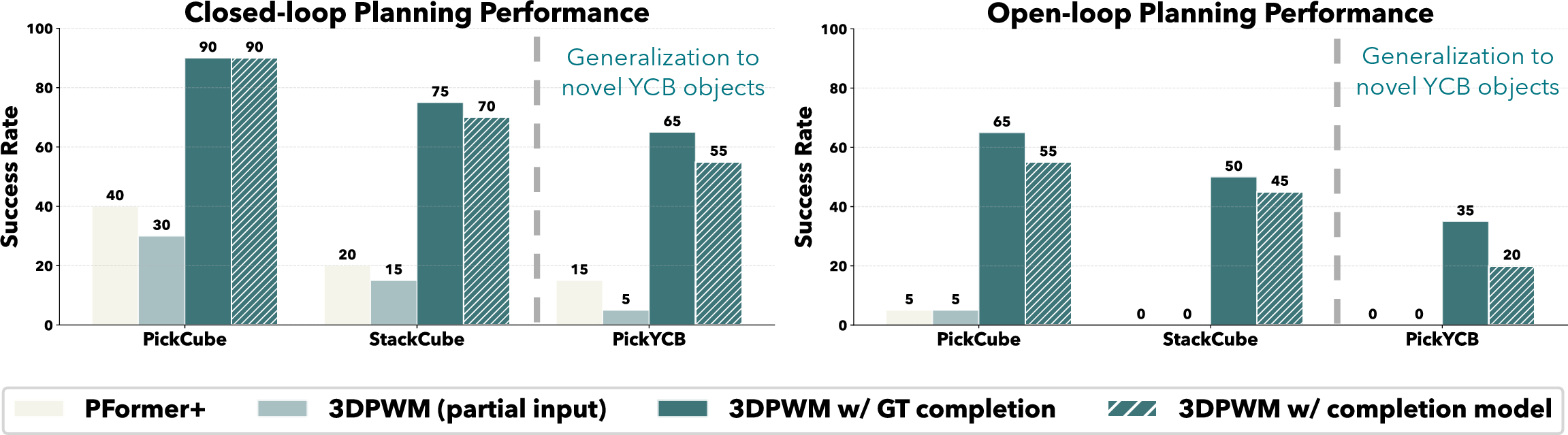
Setting. We evaluate 3DPWM under model-based planning using MPPI [49] in both open-loop and closed-loop settings on the PickCube, StackCube, and PickYCB tasks. A key motivation for learning a dynamics model is to use it as a proxy
simulator in the real world, where ground-truth observations are unavailable, making accurate open-loop control important. In the open-loop setting, the system observes only the initial point cloud and plans actions for the entire horizon, serving as a
stress test to assess whether 3DPWM can function as a robust simulator for long-horizon planning.
Baselines. Beyond ParticleFormer\(^+\)and Partial 3DPWM, we evaluate 3DPWM with ground-truth and fine-tuned point completion to quantify the impact of learned completion on planning success. This comparison quantifies the impact of learned point completion on
planning success.
Metrics. We report success rates over 20 MPPI runs, rolling out 200 samples with horizon \(H=10\) at each step, for a maximum of 100 time steps.
Results. Fig. 4 reports performance on three tasks under closed-loop and open-loop planning.
Closed-loop planning. With GT completion, 3DPWM achieves 90% success on PickCube, decreasing to 75% on StackCube and 65% on PickYCB
as task complexity increases. Learned point completion introduces a 5-10% drop on the harder tasks due to noisy completions (see Appendix 10.4). Both ParticleFormer\(^+\)and
Partial 3DPWM exhibit low success rates on partial point clouds, with ParticleFormer\(^+\)performing slightly better, likely due to its explicit
object-centric inductive bias.
Open-loop planning. All methods show a substantial drop relative to closed-loop, but 3DPWM with ground-truth completion—and to a lesser extent with learned completion—still
achieves non-trivial success rates. In contrast, ParticleFormer\(^+\)and Partial 3DPWM largely fail (1/20 on PickCube, 0% elsewhere), due to
low-quality rollout predictions leading to inaccurate cost estimation.
4.3 Adaptation to unseen long-horizon tasks.↩︎
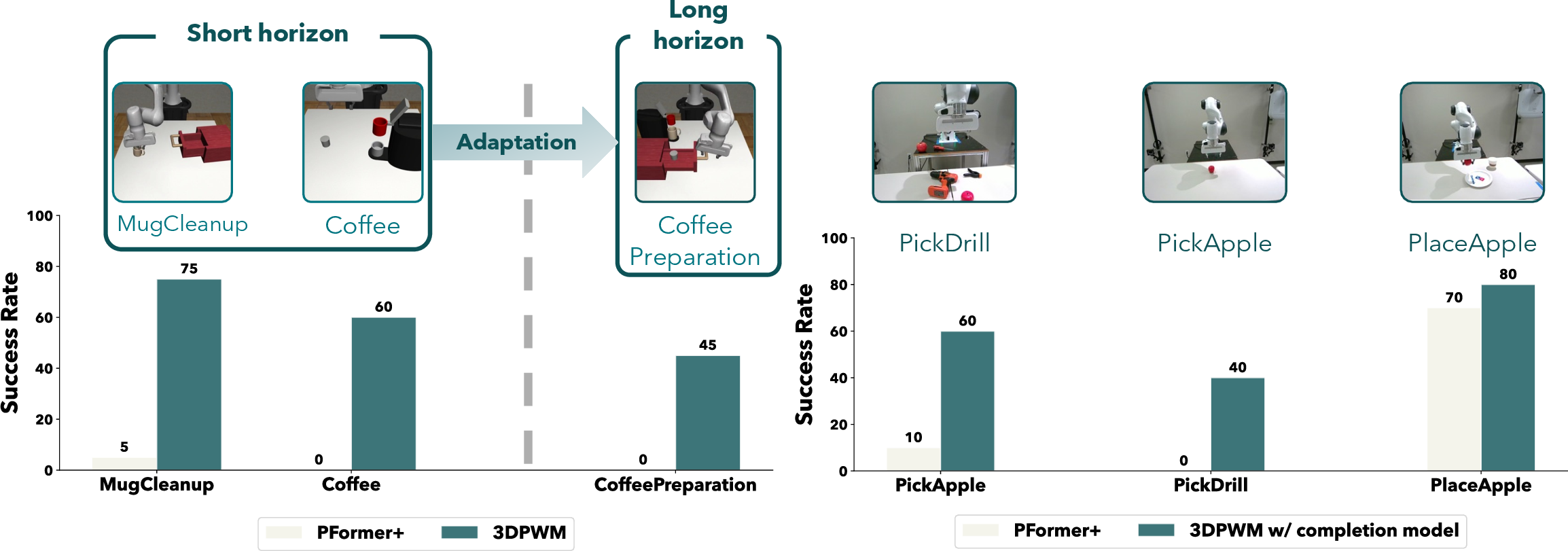
Setting. We train 3DPWM on MimicGen [51]
demonstrations for the Coffee and Mug Cleanup tasks and evaluate on Coffee Preparation, a long-horizon task requiring the robot to place a mug on the coffee machine, retrieve a pod from a drawer, load it, and close
the lid (Fig 5). This tests whether 3DPWM can compose individually learned dynamics into extended task sequences. We use ParticleFormer\(^+\) as a baseline to assess whether point completion aids generalization to new tasks.
Results. On short-horizon tasks, 3DPWM achieves 75% on MugCleanup and 60% on Coffee, with the latter’s lower performance likely due to precise
placement requirements. ParticleFormer\(^+\) performs poorly on both due to incorrect dynamic predictions. On the long-horizon CoffeePreparation, chaining the subtasks leads to a 15% drop for 3DPWM from compounding execution errors, while ParticleFormer\(^+\) fails entirely.
4.4 Sim2Real transfer of 3DPWM.↩︎
****Tasks.**** We evaluate sim-to-real transfer on tabletop Pick and Place tasks using a Franka Panda with a parallel-jaw gripper: PickApple, PickDrill, and PlaceApple (placing a toy apple onto a
plate), with randomly placed distractors. Task setups and objects are shown in Fig. 5.
System Design. We use a single-view RGB-D observation from an Intel RealSense D455 camera, extrinsically calibrated to align with the Franka base and ManiSkill2 coordinate system [53]. Target objects are segmented using SAM3 [44]
with text prompts and back-projected into 3D partial point clouds, which are then completed using a fine-tuned completion module [28]. For
dynamics, we deploy the best PickYCB checkpoint from simulation without real-world fine-tuning. Planning uses MPPI with 30–50 step open-loop rollouts executed in chunks. Additional details are in Appd. 10.2; robustness to camera viewpoints and lighting is reported in Appdx. 10.5.
Baselines & Metrics. Since Partial 3DPWM performs comparably or worse than ParticleFormer\(^+\)in simulation, we compare only against
ParticleFormer\(^+\)in real-world experiments, reporting success rates over 10 trials per method, task pair.
Results. Results are shown in Figure 5. On PlaceApple, both methods achieve comparable success (70–80%), as the plate’s large support surface yields low placement failure rates. On
PickApple and PickDrill, 3DPWM substantially outperforms ParticleFormer\(^+\), which we attribute to improved object geometry
from point completion. Remaining failures primarily arise from biased center-of-mass estimation (see Appdx. 10.4).
5 Ablation Study↩︎
We examine two key design choices in 3DPWM: the role of register tokens and the multi-step rollout length for training.
Register Tokens. We ablate the number of register tokens [47] (\(\#\text{reg}
\in \{0, 1, 2\}\)) used as keys in cross-attention alongside the action encoding \(\mathbf{z}^{\text{act}}_t\) (Table ¿tbl:tab:register95token?). Increasing from \(\#\text{reg}=0\) to \(\#\text{reg}=1\) yields substantial gains, while additional tokens show diminishing returns. We use \(\#\text{reg}=1\) for all experiments.
As discussed in Sec. 3, we hypothesize that register tokens help the model focus on task-relevant points in \(\mathbf{z}_t\) during cross-attention.
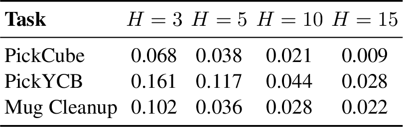
Multi-step supervision. We ablate the supervision horizon \(H \in \{3,5,10,15\}\) (Table [tbl:tab:multi95step95ablation]). Longer horizons consistently improve dynamics modeling at the cost of increased training time due to autoregressive rollouts. We use \(H=15\) for all experiments.

6 Limitations↩︎
Our system, 3DPWM, is composed of several modular components – SAM3-based object segmentation, object-centric point completion, dynamics modeling, and planning via model rollouts.
Failures in any stage can propagate through the pipeline, leading to cascading errors.
SAM failures. A common source of failure in our Sim2Real experiments was open-vocabulary object segmentation. SAM3 often failed to detect objects that were partially occluded or held by the gripper, accounting for 4/12 failures.
Point Completion Failures. Point completion was the most frequent failure mode (5/12 failed trials). The object partial point clouds obtained by back-projecting sensor depth were noisy and out of distribution for the completion module,
which was trained on individual YCB objects [54] without scene-level occlusions. Training with scene-centric partial inputs would likely improve robustness.
Latency. The modular design introduces latency at each stage. Despite the heavy segmentation backbone (848M params.), the main bottleneck is planning with the dynamics model due to sequential rollouts. We perform open-loop planning in
chunks, which works well for pseudo-dynamic tasks but limits extension to fully dynamic manipulation [55]. This latency may be mitigated
by chunked multi-step prediction [36] or lower-dimensional parametric action representations.
7 Conclusion↩︎
In this work, we demonstrate that world models based on explicit point cloud completion lead to improved rollout quality. 3DPWM achieves better predicted geometry, reward correlation,
and downstream planning performance across simulated and real tasks, including adaptation to new long-horizon tasks. Our analysis suggests tighter integration of perception components and reduced planning latency are critical directions for further
improvement.
8 Acknowledgements↩︎
The authors would like to thank the anonymous reviewers for their insightful feedback that helped improve the quality of the work. SP would like to thank Alejo for his help with Franka arm during the sim-to-real experiments, Wesley for numerous brainstorming sessions during the early stages of the project and with his help on the Point Completion codebase, Prof. Cindy Grimm for allowing us to use her lab’s Franka arm, and DMV & ViRL labmates for their feedback on the draft. This work is supported by NSF Award No. 2321851 and DARPA TIAMAT Agreement No. HR0011-24-9-0423. The views and conclusions contained herein are those of the authors and should not be interpreted as necessarily representing the official policies or endorsements, either expressed or implied, of the U.S. Government, or any sponsor.
9 Author Contributions↩︎
Skand: Led the project. Implemented the data generation pipeline for point completion and dynamics model training, trained dynamics model, and wrote the planner. Primary paper writer including figures.
Hung Nguyen: led the point completion training, and helped with sim-to-real experiments in integrating SAM3, with point completion module.
Chanho Kim: helped with writing of the paper, participated in discussions throughout the project and provided inputs on methodology.
Li Fuxin: helped with writing of the paper and provided guidance throughout the project.
Stefan Lee: helped with writing of the paper and provided guidance throughout the project.
10 Appendix↩︎
10.1 Data Generation↩︎
Point completion. We consider 100 random viewpoints for each object from the YCB dataset from which we obtain the partial point clouds inputs. A sample of the random views on three YCB objects is shown in Figure 6.

Dynamics modeling. We collect data for training the dynamics modeling with a mix of expert demonstrations as well as augment the demos with random actions to cover larger portion of the state space. Specifically, with a probability of
0.2, we select if any randomness in the expert trajectory should be induced, and if selected, we uniformly select a timestep \(i \in \texttt{0, len(traj)}\) to execute random action from step \(i\). Instead of completely using random trajectories from the beginning, our rationale to have this kind of augmentation is to induce novel collision dynamics that are unseen in the expert demonstration – such as trying to
execute a task and failing mid-way. Early on in the project, we observed that this kind of augmentation led to a dynamics model that was more performant on planning. Specifically on PickYCB, this data augmentation boosted the performance of
closed-loop planning from 58% to 65%. On PickCube the difference was similar (\(\sim\) 83% \(\rightarrow\) 90%). For all tasks across ManiSkill and DexMimicGen, we write a
custom wrapper to obtain the complete point clouds from the simulation itself by sampling points from objects/parts/geom meshes. Further, to handle point-to-point correspondences, we only sampled the points at the cannonical frame and applied rigid body
pose transformations for all the desired entities in the scene. This significantly boosted the training data collection time as well as reduced the need to store point clouds at each step (only storing one cannonical point cloud and \(\texttt{len(traj)}\) transformation matrices).
10.2 Model Details & Hyperparameters↩︎
****Point Completion.**** While complete point clouds are available from object meshes during training in simulation, we use a learned point cloud completion model at deployment time. Specifically, we fine-tune the model from [28], which is pre-trained on the ShapeNet dataset, using objects from the YCB [54] dataset. For each object, we generate partial point clouds from 100 random viewpoints, with cameras positioned on a unit-radius sphere and oriented toward the object center, and pair them with complete point clouds obtained by sampling points from the object mesh.
Furthermore, we revisit the data preprocessing and augmentation strategy. In [28], point cloud completion is formulated for upright objects in the scene by aligning each partial object point cloud input (extracted via instance segmentation) to a canonical upright orientation along the \(y\)-axis. While this simplifies learning, it restricts the ability of the model to generalize to dynamic scenarios in which objects may appear in arbitrary orientations, leading to degraded completion performance. To address this limitation, we apply rotation augmentation using all three axes (\(x\), \(y\), and \(z\)) during both pre-training on ShapeNet and fine-tuning on YCB [54]. Additionally, we apply random jittering to simulate depth noise from depth sensors. To further mitigate sensor depth noise, particularly near object boundaries and on glossy surfaces, we follow [45] to clean up boundary-related depth noise and apply a median filter to suppress noisy depth values within each object.
Data generation for training 3DPWM in simulation. For all training tasks, we use demonstrations generated in simulation. Specifically, we collect point cloud data for
training 3DPWM by replaying demonstration trajectories in the simulator and obtaining complete point clouds by sampling directly from the meshes of the objects and the robot. All actions
are recorded in delta end-effector space. Since most demonstration trajectories—particularly in ManiSkill—are generated by expert policies, they exhibit limited state-space diversity, and our initial models trained on those were not very robust. To improve
state-space coverage, we inject randomness during data collection. Concretely, for 20% of the trajectories, we randomly select a timestep and thereafter execute uniformly sampled actions for the remainder of the rollout. This simple strategy yields
partially successful trajectories that eventually fail, introducing diverse interaction and collision dynamics that are valuable for training the dynamics model.
3DPWM dynamics modeling. For training the dynamics model, we adopt the PTV3 architecture [46], replacing batch normalization with layer normalization following Sonata [56]. To better suit the smaller
dataset size, we reduce the depth of each of the four PTV3 encoding stages from the default configuration to [2,2,2,2]. Relative positional encoding (RPE) helps to capture spatial relationships between the points, but enabling it throughout
the network makes it hard to use FlashAttention [57], [58] to speed up the training process. Instead, we enable RPE in alternating encoder and decoder blocks. Accordingly, we adjust the patch size for neighborhood computation from 256 in the layers where RPE is disabled to 48
when RPE is enabled. The bottleneck per-point feature dimension is set to \(d = 256\), while the number of input points \(M\) depends on the grid resolution and scene complexity, typically
ranging from 200 to 400 points. For action conditioning, both the CrossAttn and SelfAttn modules consist of three layers with eight attention heads each. The decoder outputs 128-dimensional per-point features, which are passed
through a four-layer MLP to predict per-point velocities. Wherever applicable, we employ FlashAttention [57], [58] across all attention modules in PTV3, including the cross- and self-attention layers, to improve training efficiency. We provide detailed hyperparameters for the completion module,
dynamics training as well as for planning in Appendix 10.2. We outline the hyperparameters for all the module of 3DPWM in Table 1.
| Config/Hyperparameter | Value | |
|---|---|---|
| Point Completion | ||
| jitter prob | 0.3 | |
| jitter mean | 0.01 | |
| jitter variance | 0.03 | |
| global feature channels | 512 | |
| encoder channels | [32, 64, 128, 256] | |
| decoder upsample factors | [2, 2, 2] | |
| decoder hidden channels | 64 | |
| seed generator blocks | 4 | |
| seed generator - attn heads | 8 | |
| seed generator - attn dims | 384 | |
| seed generator - upsample factor | 2 | |
| seed generator - output dim | 256 | |
| Point Dynamics model | ||
| serialization pattern | Z + TZ + H + TH | |
| patch interaction | Shift Order + Shuffle Order | |
| positional encoding | [CPE, RPE, CPE, RPE] | |
| stride | [2, 2] | |
| encoder depth | [2, 2, 2] | |
| encoder channels | [32, 128, 256] | |
| encoder num heads | [8, 8, 8] | |
| encoder patch size | [256, 48, 256] | |
| decoder depth | [2, 2] | |
| decoder channels | [128, 256] | |
| decoder num heads | [8, 8] | |
| decoder patch size | [256, 48] | |
| mlp ratio | 4 | |
| qkv bias | True | |
| drop path | 0.3 | |
| pre norm | True | |
| shuffle orders | True | |
| MPPI Planner | ||
| planning horizon | 20-30 steps | |
| # num samples | 200 | |
| # top candidates | 64 | |
| lambda_ | 0.7 | |
| noise \(\sigma\) | 5 | |
| Training Hyperparameters | ||
| loss | HuberLoss, delta=0.25 | |
| optimizer | AdamW | |
| learning rate | 0.0001 | |
| scheduler | StepLR, step_size=30, \(\gamma=0.1\) | |
Planning computational time. On a standalone RTX-4090, planning one action takes \(\sim\)1.07s, with tasks requiring 4–5 open-loop chunks of 20 actions. Sequential dynamics rollout in observation space
is the main latency source. This can be significantly reduced via better CUDA kernels that directly chunk multi-step prediction, which we leave to future work. Training takes 12–24 hours on a single L40 GPU depending on dataset size. Datasets with larger
number of average points such as MugCleanup and with higher action space (TwoArmBoxCleanup, TwoArmDrawerCleanup) required 24 hours of training on a single GPU.
SAM3 Prompting: In this work, we assume known objects and manually prompt which object to pick and place. However, we note that this is not a fundamental limitation of the work and combination of VLMs such as Molmo [59] and segmentation methods like SAM3 [44] could automate this.
10.3 Cost Function Specification↩︎
One of the key goals of learning a point based world model in the observation space, is to be able to specify cost functions to enable planning. This requires that the rollouts produced by the dynamics model are of high fidelity – so that the cost/reward computation on the rolled out point clouds is accurate. Since we perform point completion, which enables high fidelity long-horizon rollouts, we can use cost functions which can be defined on point clouds directly. We show an example of the cost function adapted from ManiSkill [50] in a pytorch-like code [lst:pickcube_cost].
Listing lst:pickcube_cost: Cost function for the PickCube task that operates on \textcolor{PLWMcolor}{\textbf{\texttt{3DPWM}}}{}'s rolled out point clouds.
def cost_fn_pick_cube(cfg, point, info):
    """
    Cost function for the PickCube-v1 task.
    """

    goal_xyz = torch.tensor(info['extra']['goal_pos'], device=cfg.device)

    left_gripper_xyz = point['left_gripper']
    right_gripper_xyz = point['right_gripper']
    cube_xyz = point['cube']

    cube_center_xyz = cube_xyz.mean(dim=0)
    tcp_xyz = (left_gripper_xyz.mean(dim=0) +
               right_gripper_xyz.mean(dim=0)) / 2

    tcp_to_cube_dist = torch.norm(cube_center_xyz - tcp_xyz, dim=0)
    reaching_reward = 1.0 - torch.tanh(5.0 * tcp_to_cube_dist)

    cube_to_goal_dist = torch.norm(tcp_xyz - goal_xyz, dim=0)
    place_reward = 1.0 - torch.tanh(5.0 * cube_to_goal_dist)

    contact_reward = 1.0 if info['grasped'] else 0.0

    if info['grasped']:
        total_cost = -place_reward
    else:
        total_cost = -(reaching_reward + contact_reward)

    return total_cost
Since the notion of contacts is not baked in explicitly, we perform grasping when the gripper is within \(2.5\) cm of the object (i.e distance between tcp_xyz and cube_center_xyz is \(\leq 0.025\)) and assume a success (i.e info[’grasped’] = True). Alternatively, we can also try computing the intersection between the left-gripper, object and the right-gripper to determine a contact, however, in
practice we found it hard to tune the threshold for detecting the contact. We leave addressing this issue in point world models as a direction for future work.
10.4 Failure Scenarios↩︎
Point completion. First we discuss some of the failures of point cloud completion module on real world objects. We show a sample of completion success as well as failures in Figure 7. The failure scenarios primarily arise due to a mismatch between the training partial point cloud distribution and the real-world partial point cloud distribution. As mentioned in Sec. 6, our current data generation pipeline for point cloud completion does not include occlusions cause by other objects in the scene. This is because we generate partial point clouds of the objects by considering individual meshes of the objects and generating depth maps from 100 random viewpoints and backprojecting the depth to obtain the point cloud. This process, by design, does not include various kinds of occlusions caused due to the presence of other objects. Further, the noisy generation of points outside the boundary as seen in Fig 7 is also a common failure point in the pipeline.

10.5 Additional Experiments on 3DPWM robustness towards lighting conditions and camera
viewpoints↩︎
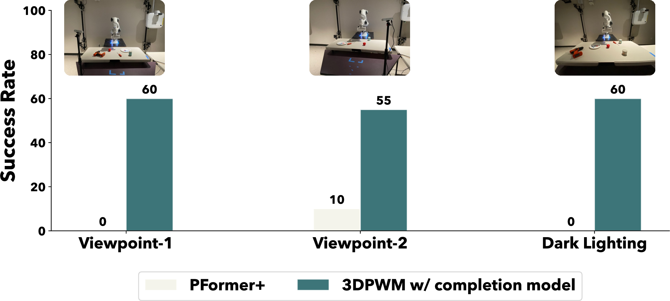
We also experimented with 2 additional camera viewpoints as well as changing the lighting conditions to test the robustness of 3DPWM. It has been shown that policies trained with
calibrated point clouds are generally more robust to such lighting and camera viewpoint changes [20], [60]. This was further corroborated by our results on PickApple shown in Figure 8. Specifically, we observe that 3DPWM maintains its higher performance when compared with ParticleFormer\(^+\).
10.6 Additional Experiments: Comparison to GNN based methods↩︎
2pt
| Task | ||||
|---|---|---|---|---|
| 2-3 (lr)4-5 | GBND [54] | GBND [54] | ||
| PickCube | 0.009 | 0.86 | ||
| Pick YCB | 0.028 | 0.85 | ||
| Box Cleanup | 0.022 | 0.83 |
Gaussian Splatting based methods like [24] comprise of (a) Gaussian point-based dynamics and (b) splatting-based rendering. Since 3DPWM focuses on modeling the dynamics and not the rendering, we compare against the GNN-based dynamics model from [24] in Table ¿tbl:tab:gbnd?. As shown in [19]
and confirmed by our results – GNN-based dynamics underperforms transformer-based approaches. Integrating a rendering pipeline into 3DPWM remains a future work that we wish to address with
3DPWM as the dynamics model.
10.7 Additional Experiments: Sim2Real in Cluttered Environment↩︎
We further evaluate the planning capabilities of 3DPWM in cluttered environments across two tasks: PickPlaceApple and StackCube. In
PickPlaceApple, the apple is initialized near a group of cluttered objects, and the cost function incorporates a heuristic penalty for collisions with surrounding objects. StackCube requires stacking a yellow cube on top of a blue
cube in a moderately cluttered environment. This task is particularly challenging, as precise placement is critical; notably, all observed failures on StackCube are near-misses, as illustrated in Figure 9
(right).

10.8 Baselines: Particleformer [19]↩︎
Here we lay out the specific details of our re-implementation of ParticleFormer [19]. Each partial point input has point
velocities and one-hot vector representing instance segmentation. We run two architecture variants (i) ParticleFormer\(^*\), which is re-implementation of the the ParticleFormer baseline with 3 transformer layers as in the
original paper, and (ii) ParticleFormer\(^+\)an equivalent variant of encoder and decoder that uses our PTV3 architecture [46].
Unlike 3DPWM, we train both these variants on segmented partial point clouds and supervise the dynamics model with the hybrid loss (a combination of Chamfer and Hausdorff losses) as
proposed by the authors.
We report the performance of ParticleFormer\(^*\) here in Table ¿tbl:tab:pformer95additional95expt? along with the copied results of ParticleFormer\(^+\)from Table
¿tbl:tab:rollout95metrics?. We find that the original ParticleFormer with 3-layers of transformer is insufficient to capture the dynamics of both PickCube as well as Box Cleanup tasks and fares lower to
ParticleFormer\(^+\).
3pt
l l c c c | c c c & & &
(lr)3-5 (lr)6-8 & & PFormer\(^+\) & & & PFormer\(^+\) & &
PickCube & 66 & 0.080 & 0.132 & 0.009 & 0.61 & 0.41 & 0.86
Box Cleanup & 218 & 0.132 & 0.225 & 0.022 & 0.30 & 0.19 & 0.83
10.9 Environments↩︎
We evaluate our dynamics model design across 6 different tasks – PickCube, StackCube and PickYCB from the Maniskill simulator [50], MugCleanup from MimicGen [51] and
TwoArmBoxCleanup and TwoArmDrawerCleanup from Dexmimicgen [52]. A sample snapshot of the environment is
shown in Figure 10.
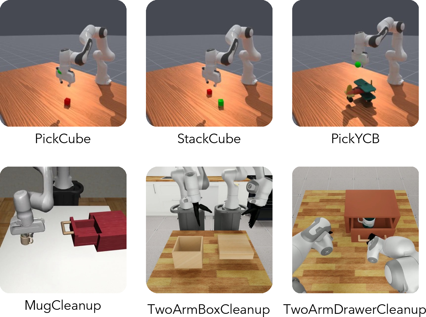
****PickCube: Lift the cube from the table to the goal position in the air specified by a 3D point in space.
StackCube: Stack the red cube on top of green cube.
PickYCB: Pick up the YCB object from the table to the goal position in the air specified by a 3D point in space.
MugCleanup: Pick and place the mug in side the drawer and close it.
TwoArmBoxCleanup: Pick up the lid of the box using two dexterous hands and place it on the box.
TwoArmDrawerCleanup: Pick and place the mug using two dexterous hands in side the drawer and close it.
For all the tasks with parallel jaw gripper, we use the end-effector delta actions, and for dexterous tasks we use 24-dim end effector actions (6-dim for pose, and 6 for finger control on each arm).
| Task | Observation Points | Action dim | |
|---|---|---|---|
| PickCube | \(1200\) | \(7\) | |
| StackCube | \(1500\) | \(7\) | |
| PickYCB | \(1200\) | \(7\) | |
| MugCleanUp | \(8192\) | \(7\) | |
| TwoArmBoxCleanup | \(10000\) | \(24\) | |
| TwoArmDrawerCleanup | \(12000\) | \(24\) |
10.10 Additional experiments we tried that did not work.↩︎
In this section we lay out some of the additional experiments we tried but did not see success and believe that this would be helpful to share with the community to improve upon.
Using SAM3D instead of custom trained point completion. We experimented with SAM3D [26] but found that the completions, while generalizable to various commonly found objects do not align with the partial input despite providing sensor depth from the camera ( instead of using DepthAnything or other foundation depth models). This is a known issue (see Issues \(\#79\) and \(\#162\) on the SAM3D github repository.)
Using Depth Foundation models to avoid noisy completions. We also tested using MOGE-2 [61] and DepthAnything3 [62] since they have shown impressive performance for depth estimation. However, we observed that while the depth was very clean and so were the resulting backprojected point clouds – these models still suffered with two major challenges which made decision making difficult: (a) similar to SAM3D, these depth foundation models suffered with object misalignment in the real world, and (b) they tended to miss out smaller details (depending on the viewpoint of the object) of the objects that could potentially be crucial for manipulation.