SWE-Router: Routing in Multi-turn Agentic Software Engineering Tasks
June 30, 2026
Abstract
Large language models (LLMs) embedded in multi-turn agentic harnesses are reshaping software engineering (SWE), but routing every task to a frontier model is wasteful when many issues admit cheap fixes. Existing LLM routers operate on the task description alone, which inherits an information-theoretic Bayes-error floor in agentic settings: a similar issue can hide either a localized typo or a multi-module refactor, and the prompt does not separate the two. We introduce SWE-Router, a value-based temporal approach that lets a cheap model run for a few exploratory turns and reads the resulting partial trajectory before deciding whether to continue cheaply or to escalate to an expensive model. We provide a Bayes-optimality theorem showing that conditioning on the partial trajectory never harms routing and is strictly better whenever exploration is informative. Across the LLM pairs of weak and strong models spanning the contemporary cost–capability frontier, we show that SWE-Router greatly improves the cost efficiency of SWE tasks, while maintaining the majority of the performances of the stronger model. We additionally release a multi-LLM trajectory dataset which allows reproduction of our trajectory-level routing.
1 Introduction↩︎
Large language models (LLMs) embedded in multi-turn agentic harnesses [1]–[4] are achieving state-of-the-art resolution rates on repository-scale coding benchmarks [5]–[7]. However, their per-task inference cost exceeds that of competitive open-weight alternatives by an order of magnitude or more, while only a minority of the existing tasks truly require frontier capability. Routing every instance to a frontier model is therefore wasteful in expectation, which motivates LLM routing [8]–[11]: selecting a model per instance so that expensive inference is reserved for cases in which it is necessary.
Existing routers operate as classifiers or calibrated probability estimators over the task description \(q\) [8], [10]–[13], picking the cheapest model whose cost-adjusted success probability is highest. This is poorly matched to multi-turn agentic SWE: a similar issue description can specify a localized typo or a multi-module refactor, and the distinction is often not identifiable from \(q\) alone. The information that resolves this ambiguity is generated by the agent itself: SWE agents follow ReAct-style loops [14] of thoughts, actions, and observations, and a substantial fraction of their turns are spent on bug localization rather than patch synthesis [3], [4]. The intermediate observations — failed tests, retrieved file contents, stack traces — supply structural signal that no prompt-only router can access.
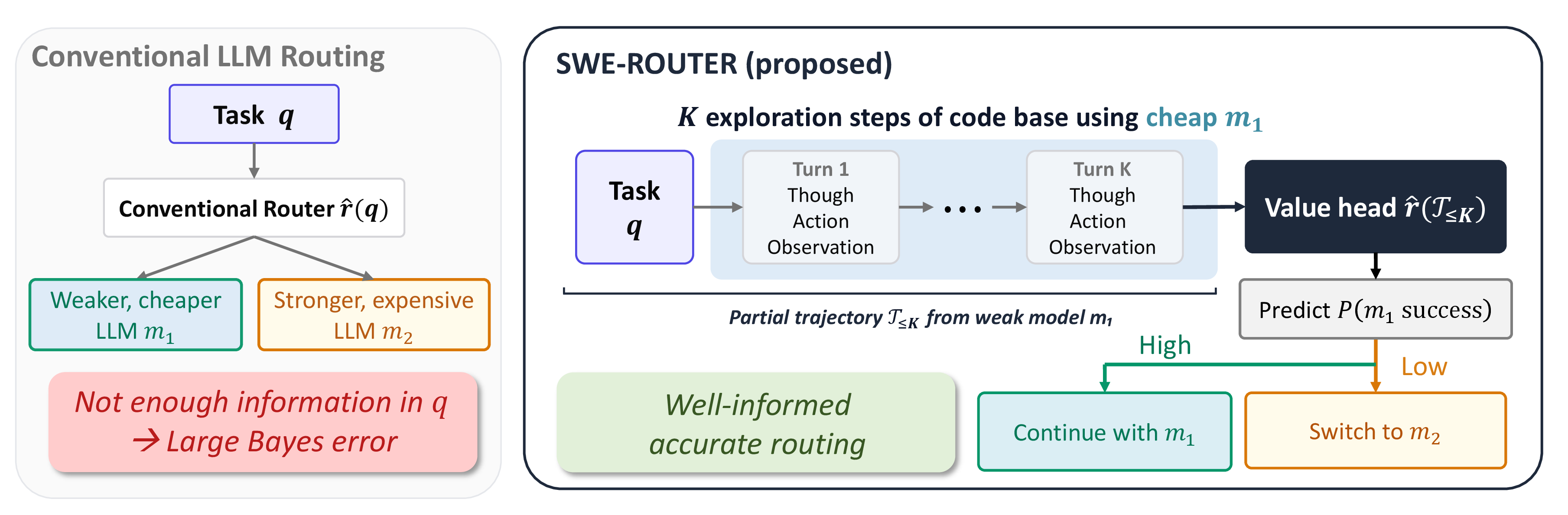
SWE-Router, our value-based temporal routing framework, operationalises this insight (1): a cheap weak model \(m_1\) runs for a few exploratory turns, then a learned value head reads the resulting partial trajectory and predicts whether \(m_1\) will eventually solve the task; if this prediction exceeds a cost-adjusted threshold, \(m_1\) continues, otherwise we escalate to a stronger \(m_2\). The value head is supervised by binary trajectory rewards and is closely related to execution-free reward models [15], but operates on incomplete trajectories and feeds a routing rule. We also provide a Bayes-optimality result (1) showing that partial-trajectory conditioning never harms routing and is strictly better when exploration is informative.
1.0.0.1 Contributions.
(i) We identify a Bayes-error floor that any prompt-conditioned router inherits in multi-turn agentic SWE, and introduce temporal routing on the partial trajectory; (ii) we instantiate this in SWE-Router, the first routing framework conditioning on the agent’s own intermediate observations; (iii) on SWEBench-Verified, SWE-Router achieves substantial cost reductions at matched resolution relative to strong prompt-only baselines.
2 Preliminary↩︎
2.1 Multi-turn Trajectories in Agentic Tasks↩︎
In agentic systems, the LLM autonomously interacts with an environment before producing a final outcome, such as the ReAct framework [14] producing a thought \(z_t\), an action \(a_t\), and an observation \(o_t\) each turn [1], [16]. Given a problem description \(q\), a
complete SWE-agent trajectory \(\mathcal{T}\) takes the form \[\begin{align} \mathcal{T}(m)=[q,\quad (z_1, a_1, o_1), \quad \ldots,\quad (z_T,a_T, o_T)],
\end{align}\] where \(m\) denotes the LLM that generated the trajectory. The final action \(a_T\) is submit, whose observation \(o_T\) is
a git patch. The patch is checked against the repository’s unit tests and assigned a verifiable binary reward \(r\in \{0,1\}\).
2.2 LLM Routing↩︎
An LLM router improves the cost–performance Pareto frontier by invoking a minimum-cost model with sufficient capability. In the binary setting it picks between a weak model \(m_1\) and a strong model \(m_2\) given \(q\) (“weak/strong” refers to cost–capability rather than parameter count); model-indexed quantities are subscripted \(1, 2\). The router invokes \(m_1\) when its cost-adjusted expected success rate exceeds \(m_2\)’s: \[\begin{align} \text{Invoke } \begin{cases} m_1 \text{ if } \hat{r}_{1}(q) - \lambda c_1 > \hat{r}_{2}(q) - \lambda c_2 \\ m_2 \text{ otherwise, } \end{cases} \label{eq:router} \end{align}\tag{1}\] where \(\hat{r}_i(q)\in[0,1]\) is the estimated probability \(m_i\) resolves \(q\), \(c_i>0\) is its expected inference cost (USD; on long agentic trajectories cost is model-dominated, so we treat \(c_i\) as \(q\)-independent). Costs are converted into success-probability units by \(\lambda>0\); tuning \(\lambda\) traces the cost–quality Pareto curve [8], [10].
In agentic settings \(q\) often does not pin down task difficulty: early turns reveal feedback (file structure, error patterns, search depth) that the issue text lacks. The decision in 1 therefore frequently inherits large Bayes error, motivating a router that can read the partial trajectory.
3 Value-Based Temporal Routing↩︎
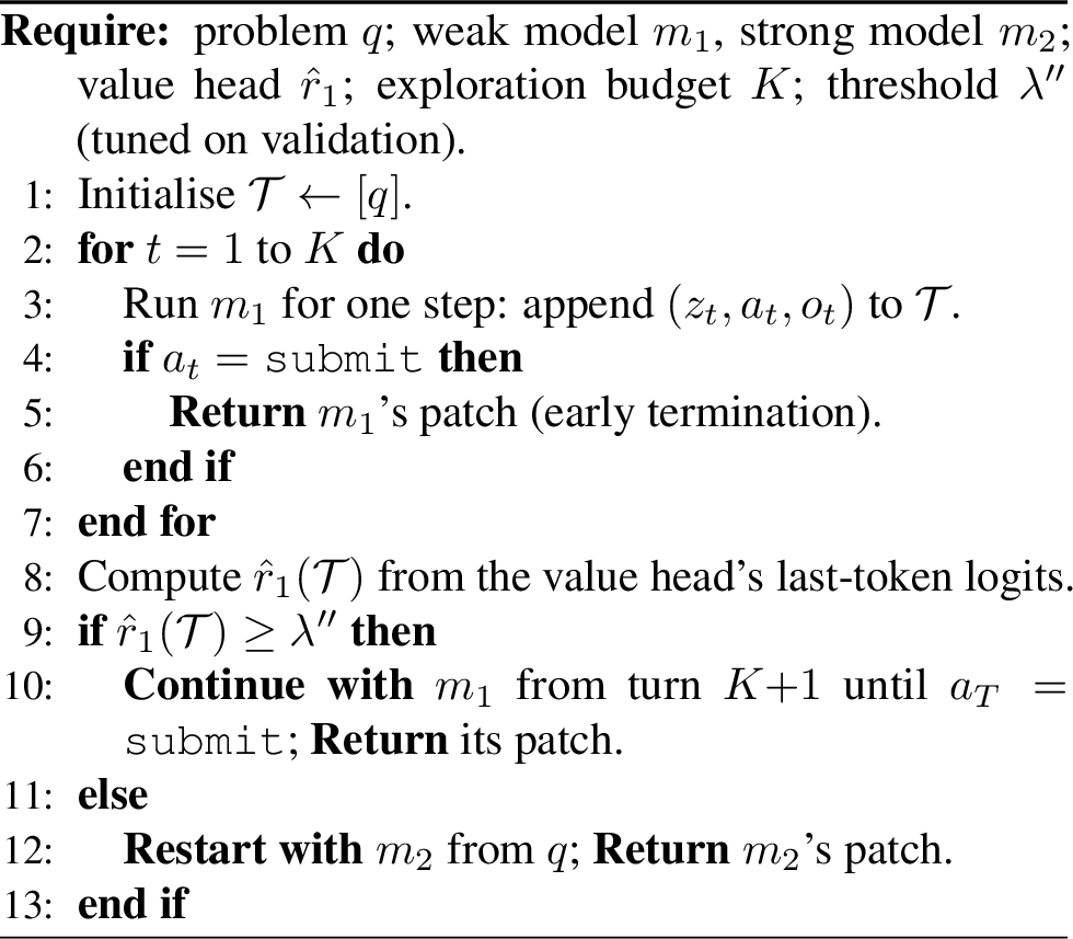
We run \(m_{1}\) for \(K\) turns to collect \(\mathcal{T}_{\leq K,1} = [q,(z_1, a_1, o_1), \ldots, (z_K,a_K, o_K)]\) and train a value function \(\hat{r}_1(\mathcal{T}_{\leq K,1})\) as a pretrained LLM with a small classification head, supervised by the binary reward \(r\) via cross-entropy. On escalation, \(m_2\) restarts from \(q\): continuation rules need expensive online \(m_2\) inference, and conditioning \(m_2\) on \(m_1\)’s reasoning has been seen to bias \(m_2\) toward \(m_1\)’s mistakes. The \(K\) weak-model turns are paid up-front and counted in any escalated run’s cost. With per-turn weak cost \(c<c_1\), the rule is \[\begin{align} \begin{cases} \text{Continue with m_1} & \text{if}\quad y_1 \geq y_2 \\ \text{Switch to m_2 from the K-th step} & \text{otherwise}, \end{cases} \label{eq:value-router} \end{align}\tag{2}\] where \(y_1=\hat{r}_1(\mathcal{T}_{\leq K,1}) -\lambda (c_1 - K c)\) and \(y_2=\hat{r}_2(q) - \lambda c_2\). SWE agents typically spend their early turns locating files and isolating failures — exploration cheaper than patch synthesis, so delegating it to \(m_1\) is a useful division of labor. Two simplifications turn 2 into a one-hyperparameter rule: (i) Threshold reduction: absorb \(\lambda(c_1{-}c_2{-}Kc)\) into a single scalar \(\lambda'\) tuned on validation, so “continue iff \(\hat{r}_1-\hat{r}_2(q)\ge \lambda'\)”; (ii) One-sided routing: treat \(\hat{r}_2\) as an unknown trajectory-independent constant, giving “continue iff \(\hat{r}_1\ge \lambda''\)”. We use one-sided routing for all reported experiments. 2 summarizes the deployment-time decision procedure.
4 Theoretical Results↩︎
Viewing routing as a one-step Bayesian decision problem, the Bayes-optimal expected utility is monotone in the conditioning \(\sigma\)-algebra. This is the classical “information never hurts” principle for Bayes decision rules [17], [18], instantiated in our trajectory-conditioning setting. Let \(Q\) be the random task description and \(S_t \mathrel{\vcenter{:}}= [Q, (Z_1, A_1, O_1), \dots, (Z_t, A_t, O_t)]\) the partial trajectory after \(t\) weak-model turns; by construction \(Q\) is a function of \(S_t\), so \(S_t\) carries strictly more information than \(Q\). The improvement is strict whenever the conditional gap \(\mathbb{E}[U_1-U_2\mid S_t]\) is not \(\sigma(Q)\)-measurable.
Theorem 1 (More informative signals improve Bayes-optimal routing). Let \(U_1, U_2\) be integrable latent cost-adjusted utilities of routing to \(m_1, m_2\), and define \(V(Z)\mathrel{\vcenter{:}}=\mathbb{E}[\max\{\mathbb{E}[U_1\mid Z], \mathbb{E}[U_2\mid Z]\}]\) for any signal \(Z\) (the Bayes-optimal expected utility under \(Z\)). If \(Q\) is determined by \(S_t\), then \(V(S_t)\ge V(Q)\).
4.0.0.1 Proof sketch.
The identity \(\max\{a,b\} = \tfrac{1}{2}(a+b+|a-b|)\) gives \(V(Z) = \tfrac{1}{2}\mathbb{E}[U_1+U_2] + \tfrac{1}{2}\mathbb{E}[|\mathbb{E}[U_1{-}U_2\mid Z]|]\). Since \(Q\) is a function of \(S_t\), the tower rule yields \(\mathbb{E}[U_1{-}U_2\mid Q] = \mathbb{E}[\mathbb{E}[U_1{-}U_2\mid S_t]\mid Q]\), and the conditional Jensen inequality applied to \(|{\cdot}|\) gives \(|\mathbb{E}[\mathbb{E}[U_1{-}U_2\mid S_t]\mid Q]| \le \mathbb{E}[|\mathbb{E}[U_1{-}U_2\mid S_t]|\mid Q]\). Taking expectations yields \(V(S_t)\ge V(Q)\). The full proof is in 10.
4.0.0.2 Practical reading.
The decomposition above clarifies why temporal routing helps. Prompt-only routers operate at the resolution of \(\mathbb{E}[U_1{-}U_2\mid Q]\), which averages out fine-grained difficulty cues only observable after a few exploratory turns. The partial trajectory \(S_t\) refines this gap: instances on which the two models would make similar predictions get routed cheaply, while hard instances are escalated. The improvement is strict whenever exploration is informative for the cost–benefit comparison; it vanishes only when the prompt already determines the optimal choice.
5 Experiments↩︎
In this section, we explain how the experiments are implemented and evaluated. We provide further details of experiment in 8 and 9.
5.1 Evaluation Metrics↩︎
Threshold-free metrics. AUROC is the standard ROC-AUC of \(\hat{r}_1(\mathcal{T}_{\le K,1})\) as a binary classifier of \(r\) and measures only the value head’s discriminative quality. Route-AUC is the normalised area under the cost–vs–resolved-rate curve obtained by sweeping the routing threshold; both axes are normalised so the all-weak point is \((0,0)\) and the all-strong point is \((1,1)\). Hence \(0\) corresponds to cost-proportional interpolation between the two LLMs and \(1\) matches the strong model’s resolved rate at the weak model’s cost.
5.2 Experiment Setting↩︎
Datasets. We use both SWE-Smith and SWE-Bench for training and test split. We only use SWE-Smith for the validation split. See 8 for further details.
LLM agents and pairs. We generate trajectories from four LLMs in mini-SWE-agent [16] and form two (weak, strong) pairs:
weak \(\in\) , and gemini-3-pro-preview for the strong model. The weak model has both lower per-instance cost and lower resolved rate in every pair (1).
Value head and training. For the value function \(\hat{r}_1\), we use Qwen2.5-Coder-7B-Instruct with a 2-class classification head fine-tuned via LoRA [19].
Baselines. Three prompt-only routers in the 1 family — logistic regression, \(k\)-NN, and XGBoost on OpenAI text-embedding-3-large embeddings of \(q\) — and our non-temporal router (\(K{=}0\) instance of our framework, conditioning only on \(q\)) are used as baselines.
5.3 Results↩︎
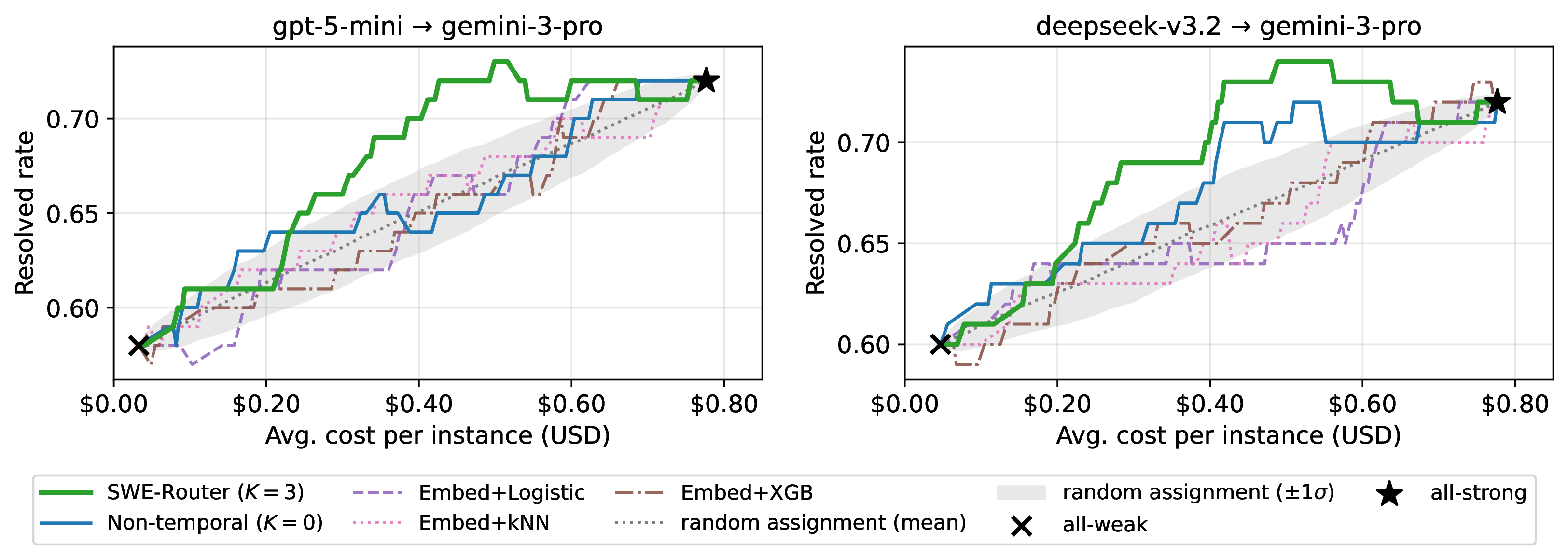
We evaluate routing on two (weak, strong) LLM pairs on the test splits of SWE-Smith and SWE-Bench datasets. We visualize the curve of routing results in 3 and compare the efficiency of SWE-Router against the baselines. The gray bands in the plots indicate the random-assignment reference, computed over \(400\) Monte-Carlo permutations of the per-instance routing decision. We also use \(\times\) and \(\bigstar\) to mark the all-weak and all-strong endpoints.
5.3.0.1 Does conditioning on the partial trajectory improve over prompt-only baselines?
The cost–resolved routing curves in 3 gives a clear summary of the advantage of using partial trajectory for temporal routing. SWE-Router (green) sits above the random-assignment band in both pairs and traces a Pareto
frontier that strictly dominates the embedding-baseline curves over most of the cost range. The picture also holds qualitatively for deepseek-v3.2 \(\to\) gemini-3-pro-preview, where the green
curve again passes above the random band at intermediate cost. We also present the computed ROC-AUC and Route-AUC values of each method in 2. In the test split of SWE-Bench Verified, both pairs show
significant improvement in Route-AUC over the baselines. When deepseek-v3.2 is used as \(m_1\), SWE-Router shows Route-AUC of \(0.780\), which is a \(+15.3\) pp improvement over the non-temporal routing baseline (\(K=0\)). While the router trained with gpt-5-mini’s trajectories for \(m_1\) also
exhibits \(+12\) pp improvement over the strongest baseline. AUROC evaluations in the test split of SWE-Bench Verified show that the accuracy of value functions are not strongly correlated to actual routing performances, as
can be shown from the AUROC of non-temporal router in the deepseek-v3.2 \(\to\) gemini-3-pro-preview pair. We further note that on both pairs the SWE-Router curve briefly passes above the
all-strong \(\bigstar\). This synergy is feasible because weak and strong solve non-identical instance subsets, so correctly routing the easy instances to \(m_1\) resolves cases on which
always-strong fails. The overall shape of the routing curves, also measured through AUC metrics in 2, is evidence that the value-head ranking captures a useful complementarity signal for efficient temporal
routing.
6 Related Work↩︎
Building on agentic frameworks like ReAct [14], recent work equips LLMs to operate on real repositories. SWE-agent [1], [16] introduces an agent–computer interface for browsing, editing, and executing code. Code benchmarks have moved from self-contained problems [20]–[22] to repository-level evaluation. SWE-bench [6] pioneered repository-scale issue resolution against hidden tests with a curated subset [23]. FrugalGPT [9] introduced cost-aware cascades, and RouteLLM [8] formalized binary routing from preference data for Pareto cost–quality gains. All the existing methods condition on the prompt alone; SWE-Router differs by conditioning on the partial agent trajectory. We provide more related works in 11.
7 Conclusion↩︎
We introduced SWE-Router, a value-based routing framework that conditions on a short partial trajectory of a cheap weak model rather than on the task description alone. A simple Bayes-optimality result (1) shows that this conditioning never harms routing and is strictly better when exploration is informative. We evaluated our approach using two pairs of popular LLMs, and showed that SWE-Router improves Route-AUC by at least \(+12\) pp on the test split of SWE-Bench Verified over the strongest baseline, also presenting the routing curve of methods where SWE-Router achieves the greatest overall performance.
Impact Statement↩︎
Our approach provides a clear positive impact of reduced frontier-model inference cost and energy use with minimal tradeoff in the overall performance. However, our proposed approach of utilizing partial trajectories can be misused to bypass safety-focused frontier models for malicious purposes. Considering multiple objectives for routing, such as considering the safety of the given task together during routing, is an important and interesting direction for future work.
8 Additional Experimental Settings↩︎
8.1 Data Collection↩︎
Training value functions requires labeled trajectory data from weaker LLMs; since SWE-smith only ships claude-3.7-sonnet trajectories [24], we generate our own and release them. 1 summarizes the collected splits.
| Dataset / Split | gpt-5-mini | deepseek-v3.2 | gemini-3-pro | |
|---|---|---|---|---|
| SWE-Smith Train | 1,692 / 33.5 / $70.1 | 1,755 / 31.9 / $85.7 | — | |
| SWE-Smith Val | 203 / 31.0 / $7.7 | 210 / 27.5 / $8.9 | 210 / 32.3 / $121.3 | |
| SWE-Smith Test | 339 / 48.7 / $11.0 | 346 / 42.7 / $13.3 | 173 / 55.4 / $95.6 | |
| SWE-Bench Verified | 500 / 55.6 / $16.6 | 500 / 62.4 / $22.6 | 500 / 70.4 / $391.3 | |
| Total cost ($) | 105.4 | 130.5 | 608.2 |
4pt
SWE-Smith instances. We sub-sample SWE-smith into three repository-disjoint partitions: train (\(\sim\)1.7k trajectories per weak LLM), val (\(\sim\)210, used for threshold tuning), and test (\(\sim\)170–346, drawn from yet another repository set). Resolved/unresolved labels come from running the SWE-smith unit tests against the agent’s submitted patch.
SWE-Bench instances. For cross-distribution evaluation we collect trajectories on SWE-bench Verified (\(500\) issues, all four LLMs). Under mix-1 (8.2), \(4/5\) of these instances enter training, so the genuinely held-out slice consists of 100 instances.
8.2 Experiment Designs↩︎
Mix-1 split constitution. Train merges SWE-Smith train trajectories with \(4/5\) of a 5-fold-CV partition of SWE-Bench Verified. We construct a validation split using the tasks from SWE-Smith, while having two separate test split from each of SWE-Smith and SWE-Bench Verified.
Value head and training. The LoRA adapter for \(\hat{r}_1\) uses \(r{=}32\), \(\alpha{=}64\), dropout \(0.05\) on attention/MLP projections. For training, we use \(5\) epochs, lr \(5\times 10^{-5}\) cosine with \(50\)-step warmup, effective batch \(16\), and context length limit of \(8192\) tokens. We use a packed procedure: one row per trajectory and the head is applied at every user-turn boundary \(K\in\{0,\dots,K_{\max}\}\) via a single shared forward pass. Each \(q\) is replaced by a uniformly-sampled paraphrase from a 3-way LLM rephrasing during training and validation, and we set \(K_{\max}=4\).
Baselines. Three prompt-only routers in the 1 family — logistic regression, \(k\)-NN, and XGBoost on OpenAI text-embedding-3-large embeddings of \(q\) — and our non-temporal router (\(K{=}0\) instance of our framework, conditioning only on \(q\)).
9 Additional Experiment Results↩︎
2 reports the full set of routing experiment results. Rows are grouped by the (weak, strong) model pair and list, in order: three prompt-only embedding baselines (Embed+LR, Embed+kNN, Embed+XGB); our non-temporal variant (\(K{=}0\)); SWE-Router with fixed budgets \(K\in\{1,2,3,4\}\). Metric semantics and the splits used in the experiment are explained in 5 and 8.
| AUROC | Route-AUC | |||||
| Method | val | SS-test | SB-V | val | SS-test | SB-V |
| \(m_1\): gpt-5-mini \(m_2\): gemini-3-pro-preview | ||||||
| Embed+LR | 0.635 | 0.692 | 0.527 | 1.140 | 0.591 | 0.565 |
| Embed+kNN | 0.629 | 0.664 | 0.563 | -0.301 | 0.604 | 0.530 |
| Embed+XGB | 0.585 | 0.589 | 0.567 | 0.782 | 0.521 | 0.517 |
| Non-temporal Router (ours, \(K{=}0\)) | 0.599 | 0.702 | 0.613 | 1.644 | 0.626 | 0.549 |
| SWE-Router fixed (\(K{=}1\)) | 0.622 | 0.679 | 0.597 | 2.358 | 0.493 | 0.702 |
| SWE-Router fixed (\(K{=}2\)) | 0.634 | 0.678 | 0.594 | 1.928 | 0.482 | 0.703 |
| SWE-Router fixed (\(K{=}3\)) | 0.631 | 0.684 | 0.586 | 1.982 | 0.547 | 0.694 |
| SWE-Router fixed (\(K{=}4\)) | 0.636 | 0.685 | 0.617 | 2.243 | 0.546 | 0.709 |
| \(m_1\): deepseek-v3.2 \(m_2\): gemini-3-pro-preview | ||||||
| Embed+LR | 0.628 | 0.660 | 0.477 | 0.455 | 0.508 | 0.476 |
| Embed+kNN | 0.600 | 0.590 | 0.489 | 0.385 | 0.444 | 0.371 |
| Embed+XGB | 0.591 | 0.618 | 0.526 | 0.430 | 0.555 | 0.465 |
| Non-temporal Router (ours, \(K{=}0\)) | 0.628 | 0.638 | 0.620 | 0.663 | 0.555 | 0.627 |
| SWE-Router fixed (\(K{=}1\)) | 0.658 | 0.649 | 0.597 | 0.646 | 0.571 | 0.768 |
| SWE-Router fixed (\(K{=}2\)) | 0.670 | 0.654 | 0.605 | 0.720 | 0.567 | 0.780 |
| SWE-Router fixed (\(K{=}3\)) | 0.666 | 0.655 | 0.603 | 0.738 | 0.547 | 0.750 |
| SWE-Router fixed (\(K{=}4\)) | 0.651 | 0.669 | 0.596 | 0.668 | 0.569 | 0.718 |
4pt
10 Proof of 1↩︎
Proof. Let \(\Delta \mathrel{\vcenter{:}}= U_1-U_2\). Using the identity \[\max\{a,b\} = \tfrac12(a+b+|a-b|),\] we obtain, for any signal \(Z\), \[V(Z) \;=\; \tfrac12 \mathbb{E}[U_1+U_2] \;+\; \tfrac12\,\mathbb{E}\!\left[\,\big|\mathbb{E}[\Delta \mid Z]\big|\,\right].\] The first term does not depend on \(Z\), so \[V(S_t) - V(Q) \;=\; \tfrac12 \left(\mathbb{E}\!\left[|\mathbb{E}[\Delta \mid S_t]|\right] \;-\; \mathbb{E}\!\left[|\mathbb{E}[\Delta \mid Q]|\right]\right).\] Since \(Q\) is a function of \(S_t\), the tower property of conditional expectation gives \[\mathbb{E}[\Delta \mid Q] \;=\; \mathbb{E}\!\left[\,\mathbb{E}[\Delta \mid S_t] \,\big|\, Q\,\right].\] Applying Jensen’s inequality with the convex function \(\varphi(x)=|x|\) conditionally on \(Q\), \[\big|\mathbb{E}[\Delta \mid S_t] \mid Q\,\big| \;\le\; \mathbb{E}\!\left[\,|\mathbb{E}[\Delta \mid S_t]| \,\big|\, Q\,\right],\] and taking outer expectations on both sides yields \[\mathbb{E}\!\left[|\mathbb{E}[\Delta\mid Q]|\right] \;\le\; \mathbb{E}\!\left[|\mathbb{E}[\Delta\mid S_t]|\right].\] Hence \(V(S_t)\ge V(Q)\), and equality holds iff \(\mathbb{E}[\Delta\mid S_t]\) is \(\sigma(Q)\)-measurable, i.e., the partial trajectory carries no information about \(\Delta\) beyond the prompt. ◻
11 Additional Related Work↩︎
LLMs for software engineering. OpenHands [2] provides an open platform for generalist software agents. Other approaches localize and patch bugs via program structure [4], simple two-stage pipelines [3], planning [25], multi-agent testing [26], or executable code actions [27]. For training, SWE-smith [24] synthesizes bug-and-fix data by injecting defects into repositories, and Agent-RLVR [28] uses execution-based RL rewards. SWE-RM [15] instead provides execution-free reward signals for patch scoring; our value head is related but operates on partial trajectories.
Software engineering benchmarks. Repository-level evaluations often involve cross-file completion [5], [29] and complex tool use [7]. SWE-bench [6] now has extensions to multimodal [30], multilingual [31], higher-rigor [32], live [33], and performance [34] settings. Since these tasks are scraped from public code, contamination is a recurring concern [35], [36], motivating contamination-resistant alternatives [37], [38]; SWE-bench Pro [39] addresses this with private repositories.
LLM routing. Existing approaches to routing between LLMs combine models of differing capability via hybrid routing [12], mixing [13], meta-modeling [40], or output ensembling [41]. Subsequent routers use contrastive embeddings [42], real-time prompt classification [43], graph formulations [44], and explicit cost or budget controls [45]–[48]; others target reasoning vs.non-reasoning routing [49]–[53] and thought-level cascades [54]. To handle unseen models, EmbedLLM [55] and universal model routing [10] embed both prompts and LLMs so routers generalize beyond training. RL-based routers [56], [57] learn multi-round or interpretable selection policies, and benchmarks [11], [58], [59] consolidate the field.