: Cheaply Evaluating Dense Supervision Signals for Long-Horizon LLM Agents
June 30, 2026
Abstract
LLM agents increasingly act over long horizons, where a single trajectory can contain hundreds or thousands of actions. In these settings, outcome-only rewards provide too sparse guidance, failing to inform the model about the goodness of intermediate actions. Dense supervision methods aim to solve this problem by scoring intermediate steps, from intrinsic confidence to self-distillation and embedding similarities. However, it is common practice to evaluate them by measuring the downstream performance of a training pipeline that integrates them. This is expensive, conflates supervision quality with training engineering confounders, and renders different methodological families requiring distinct training setups incomparable. As a result, dense supervision methods are rarely benchmarked on common ground. We introduce , a training-free testbed for directly evaluating dense supervision signals. Given a state-action pair, measures how well a method’s score is \(Q\)-aligned: whether it orders actions according to the \(Q\)-values of a strong reference-policy. This lets us compare signals before any training run and separate signal quality from other engineering choices. We instantiate as , benchmarking 21 dense supervision methods across four diverse environments and seven methodological families, with over 1.2K evaluation experiments across six open-weight model backbones. We find that simple prompting baselines consistently outperform recent dense supervision methods from the literature, and that performance clusters strongly by family. These findings hold across model sizes, environments, and observation modalities. is designed to be easily extensible to new environments and methods, enabling researchers to iterate on dense supervision methods before any training run.
0.0.1 Introduction↩︎
Large Language Models (LLMs) increasingly act as agents that write code, operate graphical interfaces, and navigate simulated environments. These are long-horizon tasks, where a single trajectory can span hundreds or thousands of actions. Sparse rewards make learning intractable as horizons grow: an outcome-based reward gives little guidance about the goodness of individual steps and, more critically, it may never be observed if the task is beyond the frontier of the model’s capabilities. Current Reinforcement Learning (RL) algorithms for LLM post-training primarily rely on sampling-based value estimation. For example, GRPO [1] estimates the value of a completion by comparing samples within a group. This works best when trajectories are short, where only a reasonable number of samples is needed to attribute which actions caused the outcome. However, agent trajectories increasingly involve multi-step tool use, recursive decomposition, and context compaction; as these grow in length outcome rewards become insufficient, and group-based estimators do not identify which actions contributed to the final outcome.
This has motivated methods that produce dense supervision signals. These include signals derived from token probabilities along reasoning traces [2], tool calls [3], or interaction feedback [4], as well as self-distillation approaches, which derive intermediate supervision from model-generated judgments or targets [5]–[7]. Although these methods differ in how they construct their scores, and have largely been developed and evaluated in isolation, they all share the goal of assigning useful values to intermediate states or actions. We therefore study them as a common class of dense supervision methods and group them into families according to how each method obtains its signal.
The primary bottleneck towards comprehensive evaluation is that we lack a cheap and direct way to compare dense supervision signals. Today, a method is evaluated by integrating it into a post-training pipeline and measuring the downstream performance improvement. This is expensive, and often unachievable due to the distinct setups required by different methods. It further makes the results hard to interpret: the measured gain conflates the supervision quality and other engineering choices used for RL training, such as algorithmic or optimization features, normalization techniques, loss-function integration strategies, and balancing with other training signals. We pose the following research question:
Can we evaluate dense supervision signals in isolation,
before any expensive post-training runs?
We introduce , a cheap, training-free testbed for dense supervision methods. This enables researchers to iterate on new approaches and their variants quickly, evaluating candidate signals before integrating them into post-training pipelines. Dense signals also matter beyond training: they can guide search at test time, including tree search or MCTS-style rollouts.
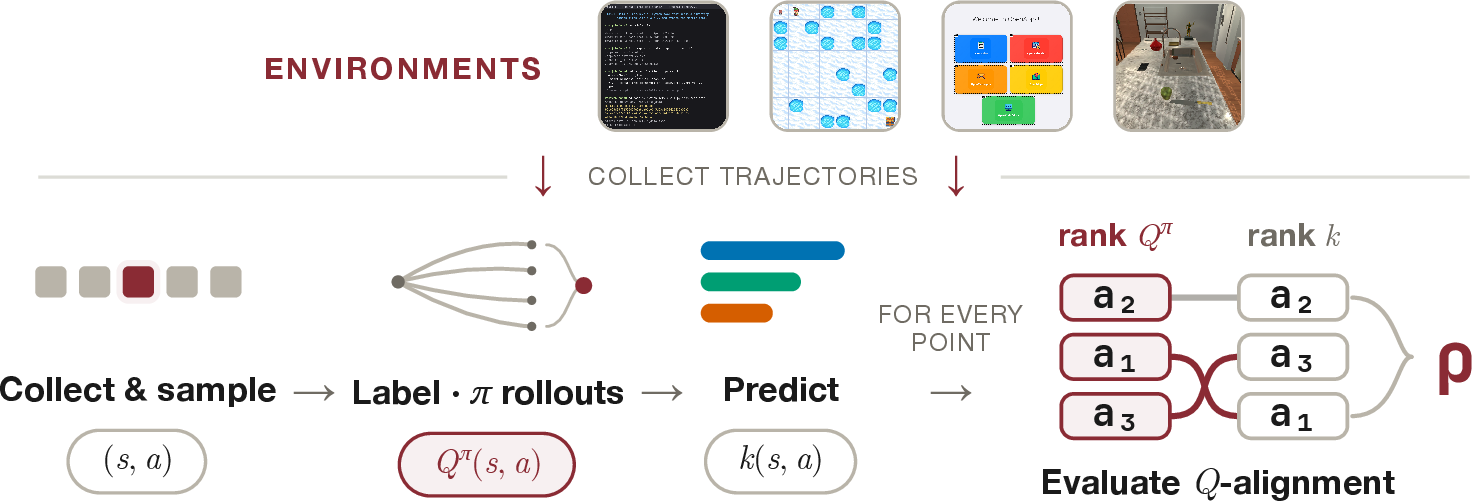
has a simple design, shown in Figure 1. For a given environment, we construct a dataset where each sample is a state-action pair \((s, a)\) labelled with a reference \(Q\)-value: the expected return of the trajectory that continues from \((s, a)\) under an expert reference policy. We obtain this expert from either an optimal policy where one exists, or a frontier model where it does not, estimating the value from the best of several rollouts (Section 0.0.3). We evaluate a method by scoring every sample by its \(Q\)-alignment: how well its predicted scores order the samples relative to the reference \(Q\)-values. Because every method sees the same inputs and is judged against the same targets, with fixed models and prompt context, isolates the quality of the signal itself from the confounders of a training pipeline, giving a cheap early indication of whether the method provides a viable learning signal.
We instantiate this methodology as , which at release covers four multi-turn environments across text and visual domains: programming and agentic terminal interaction in TerminalBench [8], computer and application use in OpenApps [9], embodied reasoning in ALFWorld [10], and goal-directed navigation in FrozenLake [11]. For each environment, we collect state-action pairs and provide reference \(Q\)-values. We use these datasets to evaluate 21 dense supervision methods spanning seven methodological families: direct prompting [12], [13], intrinsic signals [4], [14], code generation [15], [16], self-distillation [5], ranking-based prediction, pre-trained models [17], [18], and embedding similarity [19], [20].
We find substantial differences in \(Q\)-alignment across methods. Direct prompting and ranking methods perform best on average, and performance often clusters by methodological family. Code-based methods perform well in the smaller, more structured environments but weaken in the more open-ended settings we study. Added complexity within a family rarely improves alignment over simpler variants. We also find that these patterns are not explained by a single ordering of environment difficulty: different families respond differently to the state space, action space, observation modality, and available feedback. Text observations generally produce stronger alignment than image observations in our experiments, while the relative ordering of methods is largely preserved across action-value and state-value targets.
In summary, we make three main contributions. First, we introduce , a training-free testbed that evaluates dense supervision methods by their \(Q\)-alignment, how well their scores order actions according to reference \(Q\)-values, across text and visual domains (Section 0.0.2). It provides a common comparison ground, makes signal quality cheap to measure, and separates that measurement from later integration into training pipelines. Second, we explore how to annotate multimodal datasets of state-action pairs from four diverse environments, i.e., how to generate the reference \(Q\)-values, resulting in (Section 0.0.3). Third, we benchmark 21 dense supervision methods, grouped into seven families, across six open-weight backbones from 9B to 122B parameters, for more than 1.2K experiments (Section 0.0.4).
is built to grow. The same collection and labelling procedure can be easily extended to new environments. A new method only needs to provide one score per state-action pair to allow direct comparisons. We will continue expanding as new agentic benchmarks emerge. Practitioners can also use our framework to build evaluation datasets for the tasks and environments that matter in their own post-training pipelines.
0.0.2 : A Training-Free Testbed for Dense Supervision Methods↩︎
Dense supervision should primarily predict the eventual success of an agent. A single long-horizon trajectory contains many actions, and one that looks reasonable in isolation can still make the final goal harder to reach. Dense supervision methods score each intermediate action, so a score is only useful if it reflects where a decision leads rather than how good it looks locally. asks exactly this: does a method assign higher scores to the actions that make eventual success more likely?
Setup. We consider an environment modelled as a Markov Decision Process [21], with state space \(\mathcal{S}\), action space \(\mathcal{A}\), transition distribution \(T(s'\mid s,a)\), reward function \(r:\mathcal{S}\times\mathcal{A}\to\mathbb{R}\), and discount factor \(\gamma\in[0,1]\). At each step the agent observes a state \(s\in\mathcal{S}\), takes an action \(a\sim\pi(\cdot\mid s)\), receives reward \(r(s,a)\), and the environment transitions to \(s'\sim T(\cdot\mid s,a)\). A trajectory \(\tau=(s_0,a_0,r_0,s_1,\dots)\) is a realization of this process, with return \(G(\tau)=\sum_{t\ge0}\gamma^t r_t\). A policy \(\pi(a\mid s)\) maps states to distributions over actions. The \(Q\)-value function of a policy \(\pi\), \[Q^\pi(s,a)=\mathbb{E}_{\tau\sim\pi}\!\left[G(\tau)\mid s_0=s,\,a_0=a\right], \label{eq:qvalue}\tag{1}\] gives the expected return from state \(s\) after committing to action \(a\), and afterwards continuing to behave following \(\pi\) [22]. The analogous state-value function \(V^\pi(s)=\mathbb{E}_{\tau\sim\pi}[G(\tau)\mid s_0=s]\) scores a state without committing to a first action.
Reference policies. \(Q^\pi\) is only defined once a reference continuation policy \(\pi\) is fixed. uses \(Q^\pi\) similarly to how a supervised dataset uses labels, annotating each decision point with a reference value, and evaluating a method based on how well its scores reproduce their ordering. Importantly, \(\pi\) is the policy we label state-action pairs with, not the policy that will ultimately be trained with the signal. In fact, \(\pi\) should be as close to optimal as the environment allows, so that a high \(Q^\pi\) denotes a genuinely high-value action, and there is no risk of a good action receiving a bad score due to a sub-optimal continuation by \(\pi\). Outcome rewards say nothing about intermediate behaviour; \(r_t=0\) at every non-terminal step, so an action’s value is determined entirely by how \(\pi\) rolls out the trajectory. We do not assume a reference policy is available when a dense signal is later deployed, only that we can construct one here, in a controlled setting, to obtain trustworthy labels. Section 0.0.3 describes how we obtain the reference policy \(\pi\) for each chosen environment.
\(Q\)-aligned signals. A dense supervision method assigns a scalar score to each state-action pair, i.e.\(k:\mathcal{S}\times\mathcal{A}\to\mathbb{R}\). measures a single property of \(k\): whether it correlates with the reference values \(Q^\pi\), ordering decisions the same way their eventual return does when following the reference policy. Formally, we call \(k\) \(Q\)-aligned under \(\pi\) if \[k(s,a)=\phi\big(Q^\pi(s,a)\big)\quad\text{for some strictly increasing }\phi, \label{eq:q-aligned}\tag{2}\] so that a perfectly \(Q\)-aligned signal ranks all decision points exactly as \(Q^\pi\) does.
We argue that \(Q\)-alignment is a cheap proxy for a signal’s downstream usefulness, as long as the reference policy \(\pi\) used to compute \(Q^\pi\) is a close approximation of an optimal policy. A signal that orders actions by their return will provide meaningful supervision at every step a policy takes during training, and one that orders them poorly must rely on other mechanisms to be useful, so alignment is a cheap early indicator of whether a signal carries the information needed for successful supervision.
Similarly, this notion of alignment can be extended to the state-value function \(V^\pi(s)\). We discuss ’s robustness to signal types in Section 0.0.4.2.
0.0.2.0.0.1 Evaluating \(Q\)-alignment.
\(Q\)-alignment (Eq. 2 ) is a theoretical property: a signal either is a strictly increasing transform of \(Q^\pi\), or it is not. In practice, we want to measure the degree to which a method is \(Q\)-aligned under our reference policies \(\pi\). We thus evaluate each method by the rank correlation between its predicted scores and the reference labels. Predictions live on incompatible scales (e.g., raw LLM scores, code-generated outputs, token log-probabilities, embedding distances) that cannot be placed under a common loss, so we compare methods by the ordering they induce rather than by absolute values. This is consistent with recent evidence that LLM and VLM judges order candidates reliably even when their absolute scores are poorly calibrated [23]. We report Spearman’s \(\rho\) [24] as our main metric, standard for meta-evaluating an automatic scorer against reference judgments [12], and Kendall’s \(\tau\) [25] in Appendix 1.0.2. Both lie in \([-1,1]\) and measure monotonic agreement; they differ in outlier sensitivity, with Spearman dominated by a few badly-ordered pairs and Kendall weighting every inversion equally. For methods that output a permutation over the candidate actions at a state, rather than a value per point, we compute the rank correlation between the predicted and the label-induced permutation within each state and average across states. Appendix 1.0.2 gives the full definitions, including tie and NaN handling.
0.0.3 : Benchmarking Dense Supervision Methods↩︎
We instantiate the methodology as , initially employing four environments and evaluating 21 dense supervision methods, designed to be extensible beyond its initial scope. We provide an overview of the environments and methods in next, with detailed descriptions of each environment in Appendix 1.0.1 and each method in Appendix 1.0.3.
0.0.3.1 Datasets
0.0.3.1.0.1 Environments.
We choose four environments that vary in action-space structure, observation modality, and the amount of context needed to evaluate an action. The suite covers goal-directed navigation in FrozenLake [11], embodied reasoning in ALFWorld [10], browser-based computer use in OpenApps [9], and terminal-based problem solving in TerminalBench [8]. FrozenLake has four discrete actions, whereas TerminalBench accepts open-ended shell commands over rich textual observations. TerminalBench is text-only; the other environments provide both textual and visual observations. For TerminalBench, we use a subset of tasks from TBLite [26].
Data collection. For each environment, we collect trajectories and sample \(N\) state-action pairs in total (Table 2, Appendix 1.0.1). We do not aim to maximize task success during collection; instead, we prioritize diversity, including both high- and low-value states and actions. For OpenApps and FrozenLake, we use scripted policies designed to be sub-optimal to maximize coverage. For TerminalBench and ALFWorld, we generate trajectories with DeepSeek v3.2 [27]. To further improve diversity, we select a limited set of state-action pairs from a range in the middle of each trajectory. This heuristic removes data-points that carry little signal for value prediction: very early states often occur before meaningful task progress, while very late states are close to termination, so most actions have similar value. We also sample three alternative actions for each state (totalling four actions per state), which allows methods to rank candidate actions under the same context. Appendix 1.0.1, Table 2 reports the number of collected trajectories per task.
Data labeling. Our primary label is the estimated \(Q^\pi(s_t, a_t)\) under the reference policy \(\pi\) of an action \(a_t\) taken in the state \(s_t\). To label a point, we restore the environment to \(s_t\), force the first continuation step to take the dataset action \(a_t\), then follow \(\pi\) and record the discounted return. We perform this process several times if \(\pi\) is non-deterministic and choose as our label for the pair (\(s_t\), \(a_t\)) the maximum observed return as an approximation to near-optimal continuation; this corresponds to a Max-Value Monte Carlo (MVMC) sampling strategy. The reference policy \(\pi\) is environment-specific. For OpenApps and FrozenLake, we use scripted optimal policies, and for ALFWorld, we use an expert planner. In TerminalBench, however, an optimal policy is intractable to find. We therefore estimate TerminalBench values via MVMC rollouts (\(k=16\)) with GPT-5.5 [28] as a backbone. We verify that this creates a strong continuation policy: it reaches \(100\%\) Pass@16 on our TerminalBench subset, and we further compare it with Claude Opus 4.7 [29] in Section 0.0.4.2. We also provide a reference state value \(V(s_t)\) for FrozenLake, ALFWorld, and OpenApps, estimated with the same reference policies but without forcing the first action, to test whether our results are robust to the choice of target value (Section 0.0.4.2).
Appendix 1.0.3 specifies model instantiations and sampling parameters. Appendix 1.0.1 gives full environment parameterization and prompts. Appendix 1.0.5 reports complete per-model results.
0.0.3.2 Dense Supervision Methods
| Method group | Method name (source) |
|---|---|
| Ranking | ranking (Baseline) |
| Direct | direct-16 (Baseline) |
| direct-batched (Baseline) | |
| direct-sequential (Baseline) | |
| direct-single (Baseline) | |
| gvl [13] | |
| Intrinsic scoring | verifier [14] |
| \(\Delta\)belief [4] | |
| Self-Distillation | sdpo [5] |
| sdpo-gt (Extension) | |
| Pre-trained | vip [17] |
| liv-cos [18] | |
| liv-l2 [18] | |
| liv-txt [18] | |
| Embedding | vlm-sor-softmax [20] |
| vlm-sor [20] | |
| vlm-rm-cos [19] | |
| vlm-rm [19] | |
| Code | eureka [15] |
| codegen [16] | |
| codegen-avg (Extension) |
r0.55
Dense supervision methods can induce different signals and employ available information in varied ways. Using , we evaluate 21 dense supervision methods and group them into seven families by the information they use to score state-action pairs, summarized in Table 1. The methods include direct implementations of prior work, adaptations of prior methods to our setting, as well as additional baselines introduced in this paper. The latter serve either as simple baselines or as stronger probes within a method family. We next describe each family briefly.
Ranking methods prompt an LLM to directly compare a set of candidate actions from the same state. This group contains ranking, a direct LLM action-ranking baseline (details in Appendix 1.0.3.7).
Direct methods prompt an LLM or VLM to output a numeric value for a data-point. This is reminiscent of the LLM-as-judge numeric-scoring paradigm [12]. The simplest variant uses one data-point per prompt (direct-single). We also test variants that predict multiple data points at once, with points from the same environment but not necessarily from the same
trajectories. The direct-batched variant provides multiple data-points in a single prompt, while direct-sequential provides multiple data-points in a multi-turn format, appending new data-points after the previous answer. The
purpose of both variants is to test whether scoring multiple points at once helps to ground each score in a common scale. Another variant averages 16 independent estimates for the same data-point (direct-16). We also adapt GVL [13] to text-based environments and value prediction (gvl) by giving the model a shuffled full-trajectory around the target transition
before asking for a value. Appendix 1.0.3.2 gives details for these methods.
Intrinsic scoring methods derive scores from the model’s own confidence rather than from an explicit value estimate. We adapt \(\Delta\)Belief [4] (\(\Delta\)belief), which scores an action by the change in the probability the model assigns to eventual success once the action’s outcome is
observed. We also adapt LLM-as-a-Verifier [14] (verifier), which prompts the model to score a \((s,a,s')\) tuple on a rubric of per-environment quality criteria such as correctness, efficiency, and error-freeness, using the probabilities it assigns across an ordered grading scale and averaging them into a scalar
score. Appendices 1.0.3.3 and 1.0.3.4 give details on these methods.
Self-distillation methods score a candidate action by how much more likely the model is to have produced that action once it sees additional privileged information about the action’s outcome. The intuition is that a good action becomes
more probable in hindsight when its favorable outcome is shown, whereas a poor action does not. This differs from the intrinsic scoring methods, which read the model’s probability for a dedicated prompt asking about the agent’s success rather than over the
action itself. The family contains two offline re-ranking signals: sdpo [5], where the additional
information is the candidate’s immediate next state, and sdpo-gt, an oracle ablation that additionally reveals the next expert action and a summary of how the trajectory ends derived from the reference values. Appendix 1.0.3.6 gives more details for these methods.
Pre-trained methods use fixed representations from value-pretrained vision-language models. VIP [17] (vip) scores an
image state by its negative distance to a goal-image embedding. LIV [18] contributes three variants: liv-cos, which uses the paper’s
original cosine similarity score with an image goal; liv-l2, which uses a VIP-style negative Euclidean distance to an image goal; and liv-txt, which compares the state image embedding to a textual goal embedding. Appendix 1.0.3.9 provides additional details about these methods.
Embedding methods use frozen vision-language encoders to score image states by similarity to a text goal. VLM-RM [19] contributes vlm-rm-cos, which scores a state by cosine similarity between its image embedding and the goal-text embedding, and vlm-rm, which projects out baseline visual features before
measuring progress toward the goal. VLM-SOR [20] contributes vlm-sor-softmax, which uses the softmax probability assigned to
the target goal among negative goals, and vlm-sor, which thresholds that probability into a binary success reward. Appendix 1.0.3.8 provides additional details for these methods.
Code methods prompt an LLM to generate executable Python code for a scoring function with state-action pairs as input. The code is generated once and then executed to produce predicted scores for all data-points. The family contains
three methods that differ in how code is generated. codegen, our adaptation of Auto MC-Reward [16], generates \(k\) candidate functions independently (reporting per-function correlation), and codegen-avg averages their predictions first, and then reports correlation. eureka [15] instead refines the function iteratively: across several rounds, an LLM judge scores the previous round’s candidates and the best is fed back as the seed for the
next. Appendix 1.0.3.5 provides additional details for these methods.
Most methods output one score per data point. However, some methods instead output only a permutation over the candidate actions for a state (these are ranking, \(\Delta\)belief,
sdpo, and sdpo-gt). For these methods, we compute the rank correlation between the predicted permutation and the label-induced permutation within each state, then average across states. In our figures, we separate these two
categories of methods wherever applicable; we refer to the metric employed for the earlier group as global Spearman, and for the latter as state-local Spearman.
0.0.3.3 Experimental Details
Backbones. We fix the LLM/VLM backbone across methods wherever possible, so that differences in \(Q\)-alignment reflect the scoring methods themselves rather than the underlying models’ performance. We
also prioritize open-weights models with accessible internal information, so that methods requiring hidden states or token log probabilities can be evaluated. We leverage the Qwen3.5 family [30] at 9B, 27B, 35B-A3B, and 122B-A10B parameter scales, and the Gemma 4 family [31] at 26B-A4B and 31B parameter scales. The vip and liv methods use their corresponding pre-trained models. The vlm-rm and vlm-sor methods use CLIP [32] and SigLIP [33]. For the
visual ablation in Section 0.0.4.2, we use the same Qwen3.5 and Gemma 4 models.
Contextual information. To ensure a fair comparison, we give all methods the same context: a high-level task description, the same environment dynamics, a textual reward specification, and descriptions of the state and action spaces. Appendix 1.0.3 provides full prompts and parameterization details. In visual domains, we evaluate the same prompt-based method families as in the text setting; we keep the same context but provide states as images rather than textual descriptions.
0.0.4 Results↩︎
We evaluate all aforementioned methods on . We additionally complement these results with experiments testing the robustness of our conclusions and the effect of modality and signal type.
0.0.4.1 Main Results
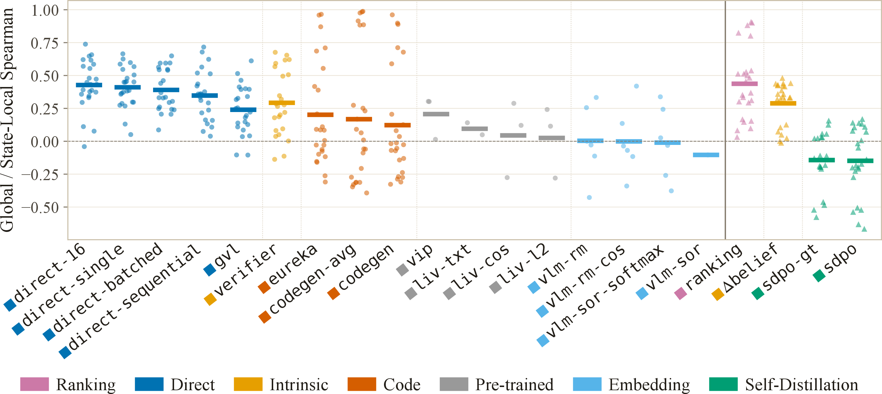
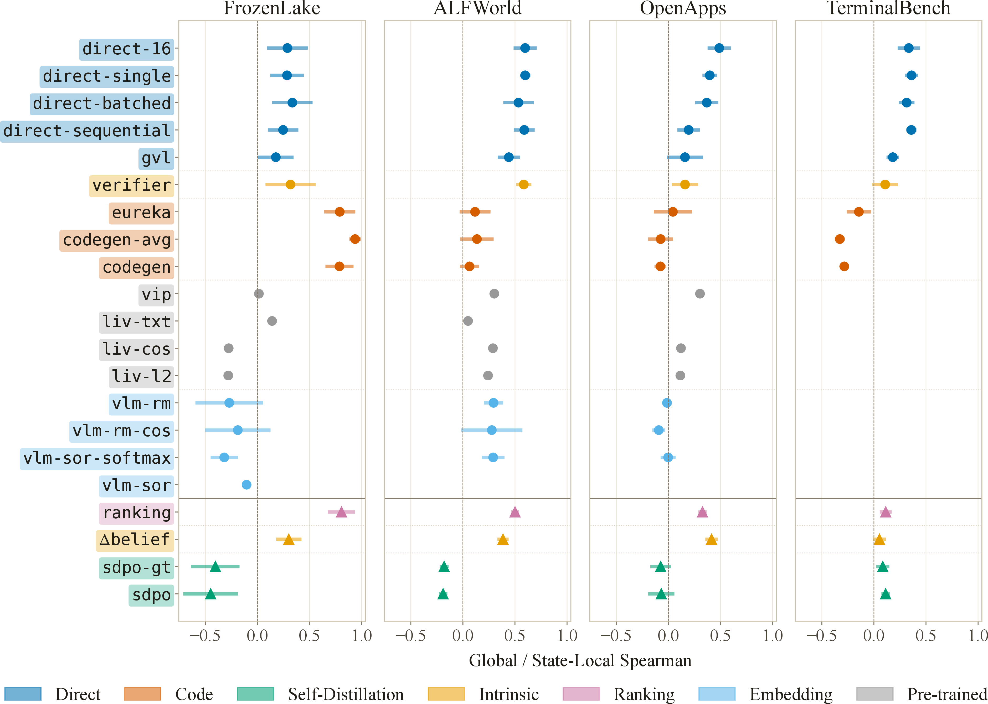
Simple methods align best. Figure 2 shows that ranking and direct prompting achieve the highest degree of \(Q\)-alignment across environments and backbones, consistently outperforming the other families. Direct value prediction is thus a surprisingly strong baseline for dense supervision. Methods also cluster clearly by family, obtaining similar correlation ranges within each, which suggests our taxonomy captures real differences in the signal each family extracts. Code-based methods are the exception, with the largest variance (Figure 3), as their effectiveness depends heavily on the complexity of the state and action spaces and on how readily those can be captured in code.
Complexity does not help. Within a family, more elaborate variants do not reliably improve \(Q\)-alignment (Figure 2). In the direct family, the multi-estimate and
batched/sequential variants do not clearly outperform the simpler direct-single. In the code family, averaging over generated functions (codegen-avg) improves the mean correlation over codegen slightly but still
leaves substantial variance. In self-distillation, giving the teacher privileged target-policy information (sdpo-gt) does not improve over sdpo. These results highlight the value of measuring signal quality directly: reveals
whether added complexity translates into a better dense feedback signal.
Difficulty does not predict performance. Figure 3 reports correlations per environment, ordered roughly from simpler closed-action settings (FrozenLake) to open-ended ones (TerminalBench) from left to right. \(Q\)-alignment does not decline monotonically with task difficulty. Direct-prompting methods stay positive everywhere, including TerminalBench, while other families behave differently for specific environments rather than following difficulty. Code and ranking methods are the clearest cases of decline, weakening in open-ended environments and turning negative for code on TerminalBench. Self-distillation works in the opposite way, with lower performance on the simple environments but stronger on TerminalBench. A method’s \(Q\)-alignment thus depends less on task difficulty alone than on the interaction with the environment’s unique characteristics.
0.0.4.2 Robustness Analyses
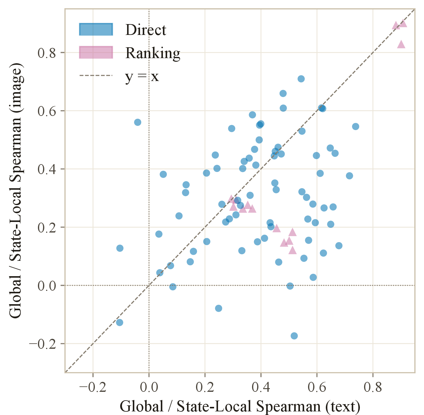

Figure 4: (Left) Text vs.image observation. Each point is an evaluation of method, environment, and model combinations. Points above the diagonal benefit from visual input; points below are hurt by it. (Right) Q-value (filled points) vs.state-value (shallow points). Signal type averaged over models & environments (OpenApps, ALFWorld, FrozenLake). Points show means; bars show ±1 SE..
Input modality. We compare \(Q\)-alignment under text and image representations of the same state, on the environments that provide both. Figure 4 (left) shows Spearman correlations per method–environment–model combination, text on the \(x\)-axis and image on the \(y\)-axis, so points below the diagonal favor text, and viceversa. The results indicate that the evaluated methods recover reference values more reliably from text than from images. This suggests that, in our setting, parsing visual information is more challenging, and the potential additional context from it does not help.
Reference value type. provides state-value labels \(V(s_t)\) alongside \(Q\)-values for OpenApps, ALFWorld, and FrozenLake, letting us test whether method rankings depend on the choice of target value. Figure 4 (right) compares the two across the direct, code, and pre-trained families, averaged over models and environments. The relative ordering of methods is largely preserved, so our conclusions do not rely on a particular value target. Absolute correlations do change: code and pre-trained methods align better with state values, direct prompting with \(Q\)-values. This likely reflects differences in how methods consume the input: code-based methods may more naturally express state-level heuristics as executable functions, while direct-prompting can explicitly prompt for a target action.
MVMC backbones. We evaluate whether the choice of backbone used for Max-Value Monte-Carlo rollout collection affects the TerminalBench labels. Figure 5 compares labels estimated using GPT-5.5 [28] and Claude Opus 4.7 [29]. Reference values from the two models result in closely matching method correlations, with methods with positive correlations under one backbone obtaining similar positive correlations under the other, and viceversa. This shows that our TerminalBench results are robust across two frontier models with independent training recipes, and the labels capture a stable notion of downstream task progress across strong model policies.
0.0.4.3 Discussion
Correlation of signals with post-training efficacy. provides a principled and cheap approach to evaluating the alignment of dense supervision methods in isolation. Nonetheless, the quality of a signal is not the only component impacting the effectiveness of RL post-training runs, and it is not isolated from the rest of the pipeline. When methods are compared directly through Q-alignment, simple direct value prediction is surprisingly competitive, outperforming more specialized mechanisms. The confounding elements we want to isolate the signal from when evaluating it (e.g., optimization and algorithmic choices, strategies for integrating the signal into the loss function, interactions with other signals, etc.) must also be studied to build successful post-training systems. Furthermore, some signals that poorly align with a particular environmental objective might still be beneficial to learning agents (e.g., exploration incentives). Therefore, future work should treat direct prompting as a baseline when evaluating signal quality.
Information across modalities. At the same time, our results must be interpreted through the information available to each method. Text-based prompting often receives compact state and task abstractions, whereas vision-only methods only receive pixels and a goal specification, making them more versatile but less performant. Their weaker alignment therefore does not show that visual feedback is intrinsically inferior; rather, it highlights that value estimation often requires the right abstraction, especially when progress depends on symbolic, relational, or hidden state information. Our robustness analyses provide early support for this view by suggesting that modality and signal type affect \(Q\)-alignment.
Overall, suggests that new dense supervision methods should justify their added complexity by improving the underlying signal, not just downstream performance, and provides a cheap diagnostic that filters candidates based on \(Q\)-alignment before expensive training runs, rather than replacing them.

0.0.5 Related Works↩︎
Evaluation through training. Most dense feedback methods are evaluated by using the proposed signal inside a downstream training or selection pipeline and reporting task return, or pass-rate improvements. For instance, self-evaluation signals that guide reasoning search are typically validated only by final task accuracy [34], and generative verifiers are assessed by downstream selection accuracy under a fixed inference budget [35]. Although this demonstrates end-to-end utility, it makes signal quality hard to isolate: measured gains depend on the policy model, optimizer, exploration process, environment distribution, amount of generated data, and implementation details of the training loop. Some work evaluates progress or reward-model quality more directly in restricted settings, especially in robotics and visual progress estimation [13], [36], [37]. is complementary: as a training-free testbed, rather than asking whether a full training recipe improves, it fixes datasets, model backbones, and environment context, then directly measures whether a proposed dense signal orders states or actions consistently with value labels derived from reference continuations.
Reward and critic benchmarks. There is also a growing literature on evaluating reward models and critic models for language and vision-language systems. RewardBench, RM-Bench, and RewardBench 2 evaluate reward models with response-comparison or accuracy-based tasks spanning chat, reasoning, safety, subtle errors, and style biases [38]–[40]. VL-RewardBench and Multimodal RewardBench extend this style of evaluation to multimodal reward models and VLM judges [41], [42]. ProcessBench and PRMBench evaluate models’ ability to identify erroneous reasoning steps [43], [44], CriticBench evaluates models’ ability to critique and correct solutions [45], while AgentRewardBench studies automatic evaluation of complete web-agent trajectories [46]. These benchmarks are closely related in spirit, but they primarily assess final responses, pairwise preferences, critiques, step-level correctness labels, or whole-trajectory judgments. instead provides a testbed for the intermediate signal needed for multi-turn agent training, measuring per-state and per-action alignment with value labels in interactive environments.
0.0.6 Conclusion↩︎
We introduce , a training-free methodology that evaluates dense supervision methods by their \(Q\)-alignment, how well their scores rank an agent’s intermediate actions according to reference values, turning a question that once required a training run into a cheap evaluation. We instantiate it as , benchmarking 21 methods spanning seven families from the literature across four environments and six open-weight backbones. We find that simple direct prompting provides the strongest signal and that methods cluster reliably by family, robustly across model sizes, environments, modalities, and target types. is built to grow: we will keep extending it with new state-of-the-art environments and domains, new methods plug in by emitting a single score per state-action pair, and practitioners can apply our methodology to build datasets for their own tasks. We hope supports faster, cheaper iteration on the dense signals needed to train long-horizon agents.
Acknowledgments↩︎
The authors thank (in alphabetical order): Hardik Bhatnagar, Nikhil Chandak, Shyamgopal Karthik, Shashwat Goel, Matthias Kümmerer, Ronald Skorobogat and Vishaal Udandarao for valuable feedback on the project. IA and JS acknowledge support by the Tübingen AI Center. JS and SHG thank the International Max Planck Research School for Intelligent Systems (IMPRS-IS) for support. SHG and AP acknowledge funding by the Federal Ministry of Research, Technology and Space (BMFTR), FKZ: 16IS24085B. AP and MB acknowledge Coefficient Giving funded by the Good Ventures Foundation. MB acknowledges funding by the Federal Ministry of Research, Technology and Space (BMFTR), FKZ: 16IS24079A. MB is a member of the Machine Learning Cluster of Excellence, funded by the Deutsche Forschungsgemeinschaft (DFG, German Research Foundation) under Germany’s Excellence Strategy – EXC number 2064/1 – Project number 390727645.
1 Appendix↩︎
We now provide thorough details about the environment, metrics, methods, and model configuration, along with complete results, which were summarized in tables.
1.0.1 Environment Details↩︎
This Appendix details the four environments comprising at release. For each, we describe the source, observation and action spaces, reward function, episode horizon, and the parameters used for trajectory collection and ground-truth labelling. Table 2 summarises the per-environment configuration; Figure 6 shows a representative state for each environment.
| TerminalBench | OpenApps | ALFWorld | FrozenLake | |
|---|---|---|---|---|
| Source | TBLite (easy) | BrowserGym suite | ALFWorld OOD | Gymnasium 8\(\times\)8 |
| Modalities | text | text, image | text, image | text, image |
| # distinct tasks | 19 | 8 | 24 scenes (1 type) | 8 maps |
| # trajectories | 118 | 40 | 40 | 50 |
| # eval points | 100 | 94 | 100 | 100 |
| # ranking points | 100 | 94 | 100 | 100 |
| Max ranking \(k\) | 4 (LLM) | 4 (manual) | 4 (LLM) | 4 (manual) |
| Episode horizon | 40 steps | 45 steps | 40 steps | 30 steps |
| Collection actor | DeepSeek v3.2 | scripted (\(\varepsilon{=}0.25\)) | DeepSeek v3.2 | scripted (\(\varepsilon{=}0.1\)) |
| Reference policy | GPT-5.5, \(k{=}16\) MC | scripted optimal | expert planner | scripted optimal |
4pt
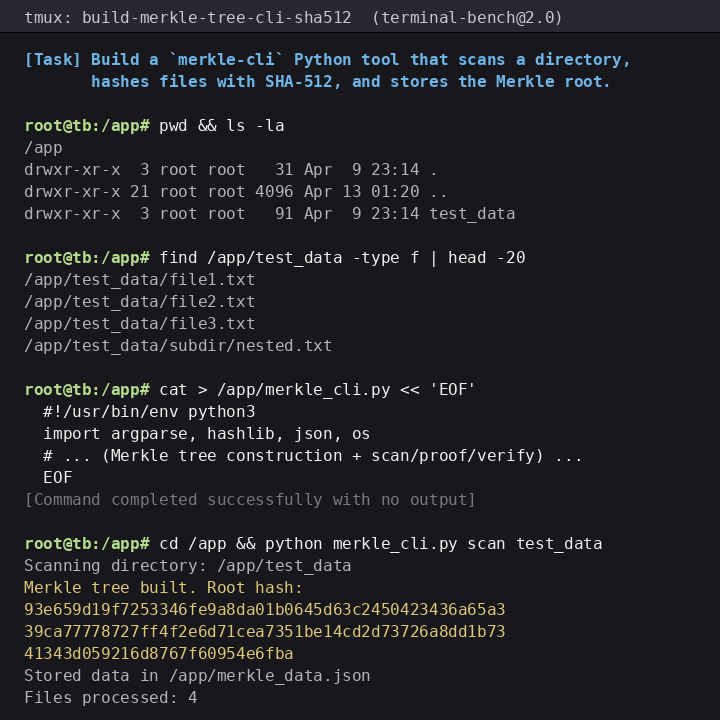

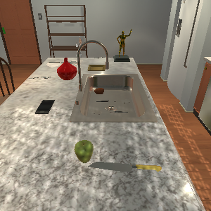

Figure 6: Representative state observations for each environment. TerminalBench is text-only and the image is for presentation only; the remaining three environments support either text or image observations, with the rendered image shown.. a — TerminalBench, b — OpenApps, c — ALFWorld, d — FrozenLake
1.0.1.1 TerminalBench
We use the easy difficulty split of TBLite [26], a curated subset of TerminalBench [8] designed for iteration on terminal agents. We specifically choose TBLite over the full TerminalBench as we find many tasks to be
unsolvable even by the best current models, mostly due to timeouts cancelling long operations (e.g., package installs in R). The split contains 19 tasks spanning system administration, cryptography, log processing, data engineering, and ML pipeline tasks.
The 19 tasks are: amuse-install, broken-python, build-merkle-tree-cli-sha512, convolutional-layers, cosign-keyless-signing, cryptographic-protocol-verifier,
hydra-debug-slurm-mode, image-tile-identification, jq-data-processing, jsonl-aggregator, log-summary, mlflow-register, pandas-etl,
playing-card-recognition, protein-sequence, raft-log-repair-concurrent-access, schedule-vacation, smiles-data-lab, systemd-log-monitoring.
1.0.1.1.0.1 Observation/Action.
The agent operates a persistent tmux-backed shell inside an Apptainer container sandbox for safety. Observations are the trailing terminal scrollback after each command; valid actions are any valid shell command (in text) wrapped in
<action> tags. Shell state (current directory, exported variables, background processes) persists across commands within a trajectory.
1.0.1.1.0.2 Reward.
Binary verifier output: \(1.0\) if the task verifier passes on submission or step truncation, \(0.0\) otherwise.
1.0.1.1.0.3 Collection.
Trajectories are collected with DeepSeek v3.2 [27] as the actor, with a maximum of \(40\) steps per episode, \(180\) s per command, and a \(900\) s wall-clock cap per trajectory. We collect \(118\) successful trajectories across the \(19\) tasks, retain one \((s, a, s')\) triple per trajectory uniformly at random (excluding the first and last \(3\) turns to avoid trivially-early and policy-saturated states), and sample \(4\) ranking-candidate actions per state from the same actor at elevated temperature (\(T{=}1.2\), top-\(p{=}0.9\)).
1.0.1.1.0.4 Reference policy.
For TerminalBench, an optimal policy would solve every task using a single, most often convoluted command; approximating such a policy would not be desirable for practical applications, as it would result in actions which are harder to interpret, less human-aligned, more error-prone, and could yield trained models that would lack the compositional skills to generalize to longer and more complex terminal-based tasks. Therefore, we choose to employ a Max-Value Monte Carlo approach: using a more desirable reference policy, we complete \(k\) trajectories from the given state and estimate the value of the data point as the highest discounted cumulative reward attained by any trajectory. In order to ensure the high quality of our labels, we constrain the reference policy to solve every task in the dataset in at most \(k\) attempts, where \(k\) is the number of rollouts sampled via Monte Carlo. For TerminalBench, we use GPT-5.5 [28] and sample \(k=16\) rollouts. We observe that GPT-5.5 obtains a Pass@16 of \(100\%\) on our subset of TerminalBench tasks. Additionally, we further validate our reference policy by showing that different models serving as the Monte Carlo backbones do not alter the results of our benchmark in Section 0.0.4.2.
1.0.1.2 OpenApps
OpenApps [9] is a suite of synthetic web applications (calendar, todo, messenger, map, code editor) built with FastHTML and
exposed through BrowserGym. The 8 tasks are: add_meeting_with_dennis (calendar), add_christmas_shopping_event (calendar), add_paper_reading_meeting_with_einstein (calendar), remove_wacv_abstract_deadline
(calendar), add_call_mom_to_my_todo (todo), mark_water_plants_as_done (todo), message_bob_to_meet (messenger), save_paris_to_my_favorite_places (map).
1.0.1.2.0.1 Observation/Action.
Each step the agent sees either an accessibility-tree (AXTree) text representation of the page or a \(1280{\times}720\) screenshot with Set-of-Marks bid annotations drawn on visible interactive elements [47]. Actions are BrowserGym primitives: click(bid), fill(bid, text), select_option(bid, option),
scroll(x, y), press(key), hover(bid), go_back(), and noop().
1.0.1.2.0.2 Reward.
The OpenApps server checks the application state against the task-specific target after every step and returns \(1.0\) once the goal state is reached, \(0.0\) otherwise.
1.0.1.2.0.3 Collection.
The collection actor is a hand-crafted scripted policy that consults the AXTree to perform each task; we mix in random BrowserGym actions with \(\varepsilon{=}0.25\) to produce a balanced mixture of successful and sub-optimal trajectories. We collect \(40\) trajectories (\(5\) per task, uniform over the \(8\) tasks), with \(\text{max\_steps}{=}45\) and a \(180\) s BrowserGym call timeout. We sample up to \(3\) evaluation points per trajectory uniformly, drop the first and last turn, and retain \(94\) \((s, a, s')\) triples and \(94\) ranking points. The \(4\) ranking candidates per state are enumerated deterministically from the live AXTree by a sampler.
1.0.1.2.0.4 Reference policy.
The same scripted policy without \(\varepsilon\)-noise serves as the optimal reference. Because the policy is deterministic and the environment is deterministic, we use a single rollout per state.
1.0.1.3 ALFWorld
ALFWorld [10] aligns the embodied THOR simulator [48] with a TextWorld interface, exposing household tasks through both natural-language observations and rendered images of the agent’s egocentric view.
1.0.1.3.0.1 Task scope.
ALFWorld defines six task types (pick_and_place, cool_and_place, heat_and_place, clean_and_place, examine_and_place, pick_two_and_place). Producing reliable expert-policy
ground-truth under the visual modality requires a planner that operates on the underlying simulator state, provided by ALFWorld. Empirically, we find the planner to be robust on pick_and_place but to degrade on the other five types when paired
with the visual rendering pipeline; to keep ground-truth quality uniformly high we therefore restrict our dataset to pick_and_place_simple. Nevertheless, task diversity within this single type is substantial: the dataset spans \(24\) distinct game files drawn from \(4\) distinct rooms (kitchen, office, bedroom-vault, bathroom) with \(8\) distinct \((\text{target
object}, \text{destination receptacle})\) pairings, including kitchen utensils placed in drawers and cabinets, writing implements on desks and shelves, valuables in safes, and toiletries in bathroom fixtures.
1.0.1.3.0.2 Observation/Action.
Text observations include the current scene description and a list of admissible commands (navigation, object pickup, placement, container open/close, object-state changes such as cleaning). In the visual modality the agent sees the egocentric THOR
render instead of the text environment description. Actions are the raw text commands wrapped in <action> tags; the adapter constrains action selection to the admissible-command set provided by the simulator.
1.0.1.3.0.3 Reward.
Binary outcome reward: \(1.0\) when the simulator declares the task goal reached, \(0.0\) otherwise.
1.0.1.3.0.4 Collection.
We collect \(40\) trajectories with DeepSeek v3.2, \(\text{max\_steps}{=}40\), sampling up to \(5\) evaluation points per trajectory uniformly with the first turn and last \(2\) turns excluded. After ranking-pruning (we keep only states with \(\geq 3\) valid alternative actions for ranking), the dataset retains \(106\) evaluation points and \(106\) ranking points; the experiments use the first \(100\). Ranking candidates (\(k{=}4\)) are sampled from the same actor at \(T{=}0.2\).
1.0.1.3.0.5 Reference policy.
We use ALFWorld’s handcoded expert planner that consults the simulator’s PDDL state to issue an optimal action sequence. The planner is deterministic, so a single rollout per state suffices. We additionally validated this reference against DeepSeek-v3.2 Max-Value MC (\(k{=}32\)): the two agree at Spearman \(0.83\) on the same evaluation points, supporting the use of the cheaper expert as canonical ground truth.
1.0.1.4 FrozenLake
We use the \(8{\times}8\) FrozenLake variant from Gymnasium [11] with deterministic dynamics
(is_slippery=False). To test agents on more than a single fixed layout, we generate \(8\) distinct random maps with seed \(42\) and cycle through them across trajectories, so
each map serves as one "task".
1.0.1.4.0.1 Observation/Action.
Text observations are an \(8{\times}8\) ASCII grid in which the agent’s current cell is marked with @, holes with H, and the goal with G; the visual modality instead provides a
\(512{\times}512\) pygame render of the same grid. The action space is four discrete moves: left, down, right, up; off-grid moves leave the agent in place.
1.0.1.4.0.2 Reward.
Sparse outcome reward: \(1.0\) for reaching the goal, \(0.0\) for falling into a hole or exhausting the step budget.
1.0.1.4.0.3 Collection.
The collection actor is a scripted shortest-path policy mixed with \(\varepsilon{=}0.1\) uniform-random noise. \(\varepsilon{=}0.1\) produces a \(\sim\!34\%\) trajectory success rate on \(8{\times}8\), sufficient to obtain a balanced mixture of successful and failed trajectories under the \(30\)-step horizon. We collect \(50\) trajectories and sample up to \(5\) points per trajectory, yielding \(239\) evaluation points; the first \(100\) are used for experiments (matching the prefix used by the other environments). Ranking candidates (\(k{=}4\)) are the four discrete actions.
1.0.1.4.0.4 Reference policy.
A scripted optimal policy that follows the shortest path to the goal serves as the reference. The environment is deterministic and so is the policy; a single rollout per state is exact.
1.0.2 Evaluation Metrics↩︎
The performance scores we provide for are correlation-based. For a dataset with \(N\) data points, let \(y_i\) denote the label associated with point \(i\) (either a state-value or a Q-value as obtained in Section 0.0.3) and \(\hat{y}_i\) the value predicted by an evaluated method. We assess methods by the alignment of \((\hat{y}_i)_{i=1}^{N}\) with \((y_i)_{i=1}^{N}\) rather than by absolute error: predictions on different scales (e.g.raw LLM scores, code-generated functions, or token log-probabilities) cannot be compared on a common loss, and the practical use of a dense signal in RL depends on the ordering the signal induces, not its numerical scale. We therefore restrict ourselves to rank-based correlation metrics.
Let \(r_i = \operatorname{rank}(y_i)\) and \(\hat{r}_i = \operatorname{rank}(\hat{y}_i)\) denote the ranks of \(y_i\) and \(\hat{y}_i\) within their respective sequences, with ties broken by averaging.
1.0.2.0.0.1 Spearman’s \(\rho\).
Spearman’s correlation [24] is the Pearson correlation [49] between the ranks: \[\rho \;=\; \frac{\sum_{i=1}^{N}(r_i - \bar{r})(\hat{r}_i - \bar{\hat{r}})}{\sqrt{\sum_{i=1}^{N}(r_i - \bar{r})^2 \;\cdot\; \sum_{i=1}^{N}(\hat{r}_i - \bar{\hat{r}})^2}}, \label{eq::spearman}\tag{3}\] where \(\bar{r}\) and \(\bar{\hat{r}}\) are the mean ranks. Equivalently, \(\rho\) is invariant under any monotonic transformation of either variable, and reduces to a sum of squared rank differences when no ties are present.
1.0.2.0.0.2 Kendall’s \(\tau\).
Kendall’s correlation [25], [50] instead counts agreements between pairs of points. A pair \((i, j)\) with \(i \neq j\) is concordant when \((\hat{y}_i - \hat{y}_j)(y_i - y_j) > 0\), discordant when this product is negative, and tied otherwise. With \(C\) concordant and \(D\) discordant pairs out of the \(\binom{N}{2}\) unordered pairs, \[\tau \;=\; \frac{C - D}{\sqrt{(C + D + T_{y})\,(C + D + T_{\hat{y}})}}, \label{eq::kendall}\tag{4}\] where \(T_{y}\) and \(T_{\hat{y}}\) are the numbers of pairs tied on the labels or on the predictions, respectively.
1.0.2.0.0.3 Comparison.
Both metrics take values in \([-1, 1]\): \(1\) denotes perfect ordinal agreement, \(-1\) a complete inversion, and \(0\) no monotonic association. They differ in what they penalise. Spearman aggregates squared rank differences, so a pair that is ordered very wrong (e.g., the largest label paired with the smallest prediction) dominates the score; Kendall counts each pairwise inversion with equal weight regardless of how far apart the points are in the ranking, making it more robust to extreme outliers but typically yielding smaller absolute values than \(\rho\) on the same data. We report both: Spearman is more sensitive to localised errors at the tails of the value distribution, while Kendall provides a stricter, scale-free reading of monotonic agreement.
If a method fails to produce a value at the point \(i\) (e.g., extraction failure for direct prediction, or a runtime error in code generation), we record \(\hat{y}_i = \text{NaN}\) and drop the pair \((y_i, \hat{y}_i)\) before computing either correlation, so the score reflects only the points the method actually attempted. Nonetheless, for every experiment, we ensure that all results we report contain a sufficient number of non-NaN points for high statistical significance.
1.0.2.0.0.4 Per-state ranking score.
The ranking methods, sdpo and ranking, do not emit a value per point but a permutation \(\sigma_i\) over the \(K_i\) candidate actions \(\{a_i^{(1)}, \dots, a_i^{(K_i)}\}\) at each state \(s_i\). We score it within each state and average across states. Let \(\sigma_i^{\star}\) be the ranking
induced by the per-candidate Q-value labels \(\{y_{i,1}, \dots, y_{i,K_i}\}\). We compute \[\bar{\rho}_{\text{rank}} \;=\; \frac{1}{|\mathcal{I}|}
\sum_{i \in \mathcal{I}} \rho\!\left(\sigma_i^{\star},\, \sigma_i\right),
\label{eq::ranking95spearman}\tag{5}\] where \(\mathcal{I}\) is the set of states with \(K_i \ge 2\) and a non-degenerate label ranking (i.e.at least two distinct \(y_{i,k}\) values). Each \(\rho(\sigma_i^{\star}, \sigma_i)\) is a Spearman correlation computed independently among the candidates of state \(s_i\), so the
metric isolates within-state action discrimination from cross-state value calibration, something the global Spearman of Eq. 3 cannot do.
1.0.3 Method Details↩︎
This Appendix details the parameterisation and execution of every method evaluated in Section 0.0.3.2. Section 1.0.3.1 fixes the contextual information shared by every prompt-based method; Sections 1.0.3.2–1.0.3.9 describe each method family; the full prompt templates are collected in Section 1.0.3.11. The complete configuration files used to launch each experiment are released alongside the benchmark.
1.0.3.1 Shared method context
Every prompt-based method receives a uniform MethodContext describing the environment, populated with per-environment data. The context contains: a one-paragraph task description, a one-paragraph reward description, a
description of the observation/action spaces, a serialised representation of the state (text or image), the most recent action (and the next state for \(Q\)-value and shaped-reward
signals), and a bounded interaction history (up to max_history_turns turns, truncated from the oldest turn first when the prompt budget is exceeded). Methods that operate on visual observations use interleaves text and image content
blocks at the positions where states and goals appear in the template. Encoder-only methods (Sections 1.0.3.8–1.0.3.9) bypass the prompt and consume the same
state/goal images directly.
1.0.3.2 Direct prediction family
All four direct variants share the same per-point prompt template (Appendix [app::prompt95direct95single]); they differ only in how many points are scored per LLM call and how the calls are batched.
1.0.3.2.0.1 direct-single.
One prompt per evaluation point. The model is asked for a single scalar inside an <answer> tag, with optional reasoning preceding it (react_tags extraction scheme).
1.0.3.2.0.2 direct-batched (packed).
Up to four points are batched into a single prompt; the model is instructed to return four scalars in order, each inside its own <answer_i> tag. The grouping is fixed at prompt_batch_size=4. We use this variant to test
whether co-presenting multiple states helps the model anchor its predictions to a common scale.
1.0.3.2.0.3 direct-sequential.
Up to eight points are presented in a single prompt as an ordered turn-by-turn dialogue: each turn shows one state-action pair and asks for one scalar before moving to the next. The ordering follows the natural temporal order of the underlying trajectory when the points come from the same trajectory; otherwise it is arbitrary.
1.0.3.2.0.4 direct-16.
Identical per-point prompt to direct-single, with \(k{=}16\) independent samples drawn at the backbone’s default decoding temperature. The reported scalar is the mean of the parsed responses; samples that
fail to parse are dropped before averaging. We use this variant to disambiguate signal quality from sampling noise.
1.0.3.2.0.5 gvl.
Our re-implementation of GVL [13] shows the model the entire trajectory in shuffled order (with no temporal markers) and asks for a per-state value scalar. We adapt the original shuffling protocol.
1.0.3.3 LLM-as-a-Verifier (verifier)
1.0.3.3.0.1 Logprob readout.
For each \((s, a, s')\) point the model is prompted with a yes/no question (“Did the agent take a high-value action?”) and we read the logprobs of the single tokens Yes and No at
the answer position, normalising via log-sum-exp: \[\operatorname{score}(s, a) =
\log p(\texttt{Yes} \mid C) -
\operatorname{lse}(\log p(\texttt{Yes} \mid C),\, \log p(\texttt{No} \mid C)).\] This requires raw token logprobs from the backbone; backbones served via OpenRouter without logprob support are therefore omitted from the verifier results.
1.0.3.3.0.2 Criteria.
Rather than a single “high-value” question, we issue one yes/no query per evaluation criterion and average their normalised scores. Criteria are environment-specific:
ALFWorld (4): correctness, error detection, efficiency, precondition awareness.
TerminalBench (3): correctness, efficiency, error detection.
OpenApps (3): correctness, efficiency, error detection.
FrozenLake (1): correctness.
Each criterion has its own one-paragraph definition surfaced inside the verifier prompt (Appendix [app::prompt95verifier]).
1.0.3.3.0.3 Prompt grouping.
prompt_grouping: random — points are shuffled before being assigned to verifier batches, eliminating trajectory-order artifacts in the cached KV state.
1.0.3.4 \(\Delta\)Belief (\(\Delta\)belief)
We adapt \(\Delta\)Belief [4] to our setting using the same logprob readout as the verifier. The model is prompted twice per \((s, a, s')\) point, once with the pre context (history up to and including state \(s\)) and once with the post context (history extended by \(a\) and \(s'\)), and asked the same yes/no question: “Will the agent eventually succeed?” The score is the change in the model’s belief after observing the action’s effect: \[\operatorname{score}(s, a, s') = \log p(\text{success} \mid \text{post}) - \log p(\text{success} \mid \text{pre}),\] with \(\log p(\text{success}\mid C) = \log p(\texttt{Yes}\mid C) - \operatorname{lse}(\log p(\texttt{Yes}\mid C),\, \log p(\texttt{No}\mid C))\). The pre/post prompt template is in Appendix [app::prompt95dbelief].
1.0.3.5 Code-generation family
1.0.3.5.0.1 codegen signature.
The model is asked to emit a single Python function whose name and signature depend on the signal type:
State-value:
signal_function(state: str) -> float.Q-value:
signal_function(state: str, action: str, next_state: str) -> float.
The prompt provides the task description, reward description, and a small number of in-context state strings drawn from collected trajectories. We sample \(k{=}16\) functions per (env, model) combination at the
backbone’s default decoding temperature, parse each via a strict signature validator, and execute them in a restricted Python sandbox. Functions that fail validation, raise during execution, or return a non-finite value contribute NaN for that
point.
We report two views of the same 16 samples: (a) codegen, the per-sample correlation, and (b) codegen-avg, in which the predictions are averaged over the 16 functions before computing the correlation, yielding a single
significance-tested cell.
We re-implement Eureka [15] as an iterative search around the codegen prompt: \(\texttt{search\_iterations}=16\) outer iterations, each generating \(\texttt{num\_samples}=8\) candidate functions; in each iteration the previous-iteration functions are scored on a
judge_num_points=8 held-out point set by an LLM judge and the best is carried into the next iteration’s prompt as a refinement target. This matches the original method modulo the LLM judge: we use the same backbone for generation and
judging.
1.0.3.6 Self-Distillation
Our offline SDPO [5] (sdpo) implementation scores candidate actions by the per-token logprob delta
between a teacher context that sees per-candidate feedback \(f\) and a student context that does not: \[\operatorname{score}(s, a) =
\frac{1}{|a|} \sum_t \big[\log p_{\text{teacher}}(a_t \mid s, f) - \log p_{\text{student}}(a_t \mid s)\big].\] Both contexts are scored on the same backbone — what distinguishes teacher from student is the prompt content, not the model. The
feedback \(f\) injected into the teacher prompt is a per-candidate textual hint derived from the candidate’s ground-truth \(Q\)-value: candidates whose GT \(Q\)-value exceeds the median in their state are marked as good candidates, the rest as bad candidates. SDPO is therefore a ranking-only method (it produces \(K\) scores per
state, not a single scalar) and is reported in the result tables under the per-trajectory ranking metric.
sdpo-gt is an oracle-teacher ablation of our offline SDPO ranking method. Like sdpo, it scores the exact same candidate action tokens under two contexts and uses the mean teacher–student log-probability difference as the action
score. The student sees only the original decision point. The teacher sees the same state plus candidate-specific evidence from cached ground-truth rollouts: the immediate next state, the next expert action after the candidate, and a compact rollout
outcome summary such as success status, remaining expert steps, and final reward. The stored GT evidence is used only as teacher prompt context.
1.0.3.7 Ranking (ranking)
The ranking method asks the LLM to score the \(K\) candidate actions available at each ranking point in decreasing order of expected value. The prompt presents the current state, the candidate actions enumerated
1..K, and asks for a comma-separated list of indices. We parse the last comma-separated permutation of \(\{1, \dots, K\}\) in the response; responses that fail to parse a valid permutation are dropped. The
reported score is the per-state Spearman of the predicted permutation against the GT-\(Q\) permutation, averaged across states with \(\geq 2\) distinct GT values. Like SDPO, the ranking
method does not produce a per-state scalar and is therefore reported only under the ranking metric.
1.0.3.8 Embedding-similarity (VLE) methods
1.0.3.8.0.1 Encoders.
Two image-text encoders are used in all four VLE variants: CLIP ViT-L/14 [32] and SigLIP-base [33]. State and goal-text inputs are encoded independently with the model’s native preprocessor; cosine similarity is computed in the joint embedding space. Both encoders are frozen.
1.0.3.8.0.2 Goal-text source.
For each environment we use a fixed target-goal description, identical across CLIP and SigLIP:
FrozenLake: “the elf reaches the gift box in the lower right corner”.
ALFWorld: the per-task
Objective:string surfaced by the simulator (e.g. “put a vase in safe”).OpenApps: the per-task goal string surfaced by the BrowserGym wrapper.
1.0.3.8.0.3 vlm-rm-cos.
Raw cosine similarity between the state embedding and the goal-text embedding.
1.0.3.8.0.4 vlm-rm.
Goal-baseline projection following VLM-RM [19]. We additionally embed an environment-specific baseline text describing a generic, goal-free state (e.g. “a blank frozen lake grid” for FrozenLake), define the direction \(\mathbf{d} = \mathbf{e}_{\text{goal}} - \mathbf{e}_{\text{baseline}}\) in embedding space, and score the state by its cosine similarity to a state-embedding shifted along that direction. The mixing coefficient is fixed at \(\alpha = 0.5\).
1.0.3.8.0.5 vlm-sor-softmax.
Continuous softmax variant of VLM-SoR [20]. The state image is scored against the target goal and a small set of negative-goal descriptions (three, per environment, e.g. for FrozenLake: “the agent fell into a hole”, “an empty frozen lake”, “a random unrelated scene”); the reported score is the softmax probability assigned to the target goal at temperature \(\tau = 0.07\).
1.0.3.8.0.6 vlm-sor.
The original thresholded VLM-SoR method: a state receives reward \(1.0\) if its softmax probability of the target goal exceeds \(\beta = 0.5\), and \(0.0\) otherwise. For state-value tables this collapses to a binary reward; we keep both the continuous and thresholded variants in the result tables to make the loss-of-information explicit.
1.0.3.9 Pre-trained value methods
1.0.3.9.0.1 vip.
VIP [17] with the original ResNet-50 checkpoint pre-trained on Ego4D. Unlike VLE, VIP is image-only: the goal is an image of the goal state.
We use the trajectory_end setting: for each evaluation point, the goal image is the rendered final state of the GT-MC reference rollout from that state, so the goal carries the same visual statistics as the state under evaluation. Scores are
negative L2 distances in the learned embedding space.
1.0.3.9.0.2 liv-cos / liv-l2.
LIV [18] in its image-goal mode, using the CLIP-RN50 LIV checkpoint pre-trained on EpicKitchens. Same trajectory_end goal-image source as
VIP. liv-cos reports cosine similarity in the LIV embedding space; liv-l2 reports negative L2 distance.
1.0.3.9.0.3 liv-txt.
LIV in its text-goal mode: the goal is the same per-environment text used for VLE (above), encoded via LIV’s text tower; cosine similarity in the joint embedding space.
1.0.3.9.0.4 \(Q\)-value evaluation.
For all encoder methods, the \(Q\)-value of a state-action pair is scored on the next state, i.e. \(\hat{Q}(s, a) = \hat{V}(s')\).
1.0.3.10 Hyperparameter summary
Table 3 lists the exact hyperparameters used for every method. Decoding parameters (temperature, top-\(p\), max-tokens, thinking budgets) are model-specific and reported in Appendix 1.0.4.
| Method | Hyperparameter | Value |
|---|---|---|
| direct-single | samples / point | 1 |
| direct-batched | batch size | 4 (packed) |
| direct-sequential | batch size | 8 (sequential turns) |
| direct-16 | samples / point | 16 (averaged) |
| gvl | shuffled context size | full trajectory |
| verifier | criteria | env-specific (1–4) |
| verifier | prompt grouping | random |
| \(\Delta\)belief | criterion | “will eventually succeed” |
| codegen | samples (functions) | 16 |
| codegen-avg | aggregator | mean over 16 |
| eureka | search iterations | 16 |
| eureka | samples per iter | 8 |
| eureka | judge held-out points | 8 |
| sdpo | feedback type | per-candidate good/bad |
| ranking | parser | last permutation of \(\{1..K\}\) |
| vlm-rm | \(\alpha\) | 0.5 |
| vlm-sor-softmax | \(\tau\) | 0.07 |
| vlm-sor | \(\beta\) (threshold) | 0.5 |
| vlm-sor* | negative goals | 3 per env |
| vip | backbone | ResNet-50 (Ego4D) |
| vip | goal source | trajectory_end image |
| liv-cos, liv-l2 | backbone | CLIP-RN50 (EpicKitchens) |
| liv-cos, liv-l2 | goal source | trajectory_end image |
| liv-txt | goal source | per-env target-goal text |
4pt
1.0.3.11 Prompt templates
We list one representative prompt per method family. Templates use {slot} for runtime substitutions; literal tags such as <system>,
<user>, <assistant>, <answer>, and <score_1> are emitted verbatim. The prompt boxes use the shared promptlst listings style: role tags are written literally, and
placeholders are injected with (*@\promptslot{slot}@*). The shared direct, GVL, verifier, codegen, and ranking builders are taken from src/value_bench/prompts.py; method-specific wrappers are taken from
src/value_bench/methods/delta_belief_ranking.py, src/value_bench/methods/sdpo_ranking.py, and src/value_bench/methods/llm_eureka.py at the release commit.
The prompt-driven methods in Table 1 are covered as follows: direct-single, direct-16, direct-batched, and direct-sequential share the direct template with
different batching wrappers; gvl, verifier, \(\Delta\)belief, sdpo, sdpo-gt, ranking, codegen, codegen-avg, and
eureka have separate entries below. The pretrained and embedding methods (vip, liv-*, vlm-*) do not emit LLM prompt templates in this codebase.
Prompt C.1: direct-single, \(Q\)-value, optimal-policy assumption <system> You are an expert at estimating Q-value functions for reinforcement learning environments.
The Q-value Q(s,a) represents the expected (*@ {}@*) when taking action a in state s and then following the optimal policy thereafter. In other words, Q(s,a) is the expected return given that action a is taken in state s, assuming optimal play thereafter. It depends on both the state and the specific action taken.
(*@ {}@*)
You will receive the episode’s state-action history (if any), the current state, the action taken, and the resulting next state. Estimate Q(s,a) for the Current Action in the Current State – the expected (*@ {}@*) when taking this action in this state, assuming optimal play thereafter. The history provides context about how the agent reached the current state.
(*@ {}@*)
(*@ {}@*)
(*@ {}@*)
(*@ {}@*)
After any reasoning, respond with ONLY a single numeric Q-value estimate. Do not include any explanation after your final number. </system>
<user> Estimate the Q-value for the Current Action in the Current State for the following:
(*@ {}@*)
### State-Action History
[Note: Only the last (*@ {}@*) of (*@ {}@*) turns are shown.]
[Turn (*@ {}@*)/(*@ {}@*) - State] (*@ {}@*)
[Turn (*@ {}@*)/(*@ {}@*) - Action] (*@ {}@*)
### Current State [Turn (*@ {}@*)/(*@ {}@*)] (*@ {}@*)
### Current Action (*@ {}@*)
### Next State (*@ {}@*)
Now, provide your Q-value estimate as a single number. Do not explain – output ONLY the number. </user>
direct-batched and direct-16 prepend Estimate ... for each datapoint below, wrap each example in ## Datapoint i, and ask for a comma-separated list of numeric Q-value estimates in datapoint order.
direct-sequential instead sends one user turn per datapoint, headed ## Datapoint i of n, and asks the model to keep earlier estimates fixed while returning exactly one estimate for the current turn.
Prompt C.2: gvl, shuffled-trajectory value elicitation <system> You are an expert at estimating Q-value functions for reinforcement learning environments.
(*@ {}@*)
You will receive the current state, the action taken, and the resulting next state. Estimate Q(s,a) for the Current Action in the Current State – the expected (*@ {}@*) when taking this action in this state, assuming optimal play thereafter.
(*@ {}@*)
You will receive a shuffled set of surrounding transitions from the same trajectory, followed by one final target datapoint. The surrounding transitions are intentionally out of chronological order and are provided only as contextual evidence. Estimate only the final target datapoint.
Only the target datapoint includes its resulting next state. Surrounding context transitions include only state and action.
After any reasoning, respond with ONLY a single numeric Q-value estimate. Do not include any explanation after your final number. </system>
<user> Estimate the Q-value for the Current Action in the Current State for the following:
(*@ {}@*)
## Shuffled Trajectory Context The surrounding transitions below come from the same trajectory as the target datapoint, but are intentionally shuffled and not chronological.
### Context Transition (*@ {}@*) #### State (*@ {}@*)
#### Action (*@ {}@*)
## Target Transition ### Target State (*@ {}@*)
### Target Action (*@ {}@*)
### Target Next State (*@ {}@*)
Now, provide your Q-value estimate as a single number. Do not explain – output ONLY the number. </user>
Prompt C.3: verifier, score-bin with logprob readout <system> You are an expert verifier for reinforcement learning environments. Estimate Q-value using an ordered discrete score scale.
(*@ {}@*)
You will receive the episode’s state-action history (if any), the current state, the action taken, and the resulting next state. Estimate Q(s,a) for the Current Action in the Current State – the expected (*@ {}@*) when taking this action in this state, assuming optimal play thereafter. The history provides context about how the agent reached the current state.
Use an ordered 20-point score scale with the single-letter bins A through T, where A is best and T is worst. Choose exactly one score bin per datapoint. A = clearly and completely favorable with strong evidence of success (best) B-D = strongly favorable with only minor remaining concerns E-G = above average, mostly favorable with some issues H-J = uncertain, leans favorable K-M = uncertain, leans unfavorable N-P = below average, significant issues remain Q-S = poor, with only limited signs of progress T = clearly and completely unfavorable or failed (worst)
Interpret the score bins as an ordered scale that will be converted into a scalar value after decoding. Use higher bins for stronger evidence that the state or chosen action is favorable.
(*@ {}@*)
Return exactly one score tag for the single datapoint. </system>
<user> Estimate a verifier score for each datapoint below. Estimate the Q-value for the Current Action in the Current State. Judge the chosen action and resulting next state using the ordered score bins.
### Evaluation Criterion: (*@ {}@*) (*@ {}@*)
## Datapoint 1
(*@ {}@*)
Now provide your final scores using one uppercase letter from A through T per datapoint. Output exactly one tag per datapoint in prompt order:
<score_1>LETTER</score_1> </user>
Prompt C.4: \(\Delta\)belief, pre/post belief query <system> You are an expert at judging how candidate actions change an agent’s probability of eventual success in a sequential decision-making
environment.
(*@ {}@*)
Interpret "successful overall outcome" using the task and reward function below. For sparse-success tasks, this means eventually completing the task. For dense-reward tasks, this means achieving a strong overall return.
Each candidate is scored by the change in log-probability of the one-word answer "Yes" to a success question after the candidate’s observed outcome is revealed.
(*@ {}@*) </system>
<user> Assess the current situation before any candidate outcome is shown.
(*@ {}@*)
**Current State:** (*@ {}@*)
Do not answer directly. The assistant continuation being scored is the one-word answer to the success question below.
Question: Given the task and reward function, is the agent likely to eventually achieve a successful overall outcome from here, assuming optimal future decisions thereafter? Answer with exactly one word: Yes or No. </user>
<user> Re-assess the same situation after one specific candidate action has been attempted and its observed outcome is available.
(*@ {}@*)
**Current State:** (*@ {}@*)
**Candidate Action:** (*@ {}@*)
**Observed Resulting State:** (*@ {}@*)
Do not answer directly. The assistant continuation being scored is the one-word answer to the success question below.
Question: Given the task and reward function, is the agent likely to eventually achieve a successful overall outcome from here, assuming optimal future decisions thereafter? Answer with exactly one word: Yes or No. </user>
Prompt C.4 scored continuations <assistant> Yes </assistant>
<assistant> No </assistant>
The backend scores the continuations Yes and No; the method uses the post-minus-pre log probability of Yes.
Prompt C.5: codegen, signal-function generation <system> You are an expert at writing Q-value functions for reinforcement learning environments.
(*@ {}@*)
(*@ {}@*)
(*@ {}@*) </system>
<user> Write a Python function that estimates the Q-value for a given state, action, and next state.
The function signature must be:
“‘python def signal_function(state: str, action: str, next_state: str) -> float: “’
The function receives text representations of the state, the action taken, and the resulting next state. It should return a float representing the estimated Q-value.
Important constraints: - Do NOT use recursive search, tree expansion, lookahead, or any form of simulation/rollout – these will time out. - Base the estimate on direct analysis of the state representation, using your understanding of what features predict good outcomes.
You may use the ‘collections’, ‘itertools’, ‘json’, ‘math’, ‘re’, ‘statistics’, and ‘string’ standard library modules. The function will run in a restricted sandbox that does not expose the introspection builtins ‘locals’, ‘globals’, ‘vars’, ‘dir’, ‘eval’, or ‘exec’ – calling any of them raises NameError at runtime, so do not rely on them. After any reasoning, output ONLY a single Python code block containing the function definition. No explanations or commentary after the code block. </user>
codegen-avg uses the same generation prompt for multiple independent samples and averages the resulting predictions over valid generated functions.
Prompt C.6: sdpo, asymmetric teacher / student contexts <system> You are an expert at comparing and ranking actions by their Q-value in reinforcement learning environments.
(*@ {}@*)
You will evaluate one fixed candidate action at a time. The base policy scores the candidate from the original state. A self-teacher may additionally see environment feedback produced after that same action was attempted, and should use that feedback as per-turn evidence about whether the original action improved expected future success from the current state.
(*@ {}@*)
(*@ {}@*) </system>
<user> (*@ {}@*)
(*@ {}@*)
**Current State:** (*@ {}@*)
(*@ {}@*) </user>
<user> (*@ {}@*)
(*@ {}@*)
**Current State:** (*@ {}@*)
(*@ {}@*) (*@ {}@*)
(*@ {}@*) </user>
Prompt C.6 scored continuation <assistant> (*@ {}@*) </assistant>
For the base sdpo method, the feedback text is the serialized resulting state for the candidate action when next-state feedback is enabled; otherwise the prompt emits [No explicit feedback was available for this action.]. The
same candidate action is scored in the student and teacher contexts; the method uses teacher-minus-student mean token log probability.
Prompt C.7: sdpo-gt, oracle teacher with stored expert evidence <system> You are an expert at comparing and ranking actions by their Q-value in reinforcement learning environments.
(*@ {}@*)
You will evaluate one fixed candidate action at a time. The base policy scores the candidate from the original state. A self-teacher may additionally see environment feedback produced after that same action was attempted, the next expert action from the resulting state, and a compact stored expert rollout summary. It should use that privileged evidence to judge whether the original action improved expected future success from the current state.
(*@ {}@*)
(*@ {}@*) </system>
<user> (*@ {}@*)
(*@ {}@*)
**Current State:** (*@ {}@*)
(*@ {}@*) </user>
<user> (*@ {}@*)
(*@ {}@*)
**Current State:** (*@ {}@*)
(*@ {}@*) (*@ {}@*)
(*@ {}@*) The (*@ {}@*) below occurs after the (*@ {}@*) has already been executed in the (*@ {}@*). Use it only as evidence about the original (*@ {}@*); it is not a replacement command to output. (*@ {}@*): (*@ {}@*)
Structured stored expert rollout summary: (*@ {}@*): (*@ {}@*) (*@ {}@*): (*@ {}@*) Remaining distance proxy: (*@ {}@*) (*@ {}@*): (*@ {}@*) Stored ranking GT value ((*@ {}@*)): (*@ {}@*) Stored expert rollout outcome: (*@ {}@*)
(*@ {}@*) </user>
Prompt C.7 scored continuation <assistant> (*@ {}@*) </assistant>
The runtime headings and labels specialize to the environment. For example, TerminalBench uses shell-response, expert-command, verifier-success, and verifier-reward labels; OpenApps, ALFWorld, and FrozenLake use the corresponding browser, household-command, or grid-move labels.
Prompt C.8: ranking, candidate-permutation request <system> You are an expert at comparing and ranking actions by their Q-value in reinforcement learning environments.
(*@ {}@*)
You will receive the episode’s state-action history (if any), the current state, a list of candidate actions, and the resulting next state for each action. Rank the actions by their expected Q-value Q(s,a) – the expected (*@ {}@*) when taking each action. Output the action numbers from best to worst.
(*@ {}@*)
After any reasoning, output ONLY a comma-separated list of action numbers from best to worst. For example: 2, 1, 3, 4. </system>
<user> Rank the following actions by Q-value (best to worst) for the Current State:
(*@ {}@*)
(*@ {}@*)
## Current State [Turn (*@ {}@*)/(*@ {}@*)] (*@ {}@*)
The following candidate actions are being evaluated in the current state:
## Actions to rank
[**Candidate Action (*@ {}@*)**] (*@ {}@*)
[**Resulting State (*@ {}@*)**] (*@ {}@*)
Rank all listed actions ((*@ {}@*) total here) from best (highest Q-value) to worst. Output ONLY a comma-separated list of action numbers. For example: (*@ {}@*). </user>
Prompt C.9: eureka, iterative code search with LLM judging <system> You are an expert at writing Q-value functions for reinforcement learning environments.
(*@ {}@*)
(*@ {}@*)
(*@ {}@*)
## Iterative Search You are participating in an iterative code-search loop. Each proposed candidate will be executed on benchmark datapoints, judged from its predicted values, and the winning code plus feedback may be shown back to you in the next iteration. Improve usefulness of the signal based on behavior, not code aesthetics. </system>
<user> ## Search Iteration Iteration (*@ {}@*) of (*@ {}@*). Write one candidate Python function for estimating the Q-value.
## Function Contract The function definition must start with:
“‘python def signal_function(state: str, action: str, next_state: str): “’
The function may return either: 1. a single float, which is the actual signal value 2. a tuple ‘(float, dict[str, float])’ where the first float is the actual signal value and the dictionary contains named additive components used only for search-time feedback.
If you return a dictionary, use short stable snake_case keys and make the scalar total equal to the sum of the component values. Build the components dictionary with explicit literal keys – do NOT use ‘locals()’, ‘globals()’, or ‘vars()’.
## Return Example “‘python def signal_function(state: str, action: str, next_state: str): progress_reward = 0.4 safety_penalty = -0.1 total = progress_reward + safety_penalty return total, "progress_reward": progress_reward, "safety_penalty": safety_penalty, “’
## Current Best Code (*@ {}@*)
## Judge Feedback (*@ {}@*)
(*@ {}@*) </user>
<system> You are selecting the most useful dense-signal candidate for a reinforcement learning environment.
(*@ {}@*)
Judge candidate behavior from predicted values and diagnostics. Do not infer quality from code style because candidate code is not shown.
(*@ {}@*) </system>
<user> ## Selection Rule Choose the candidate whose predictions are the most appropriate and useful Q-value estimates. Prefer candidates that provide discriminative, stable, non-collapsed values and that match the intended semantics of the signal on the sampled datapoints.
## Candidate Summaries ### Candidate (*@ {}@*) - Finite predictions: (*@ {}@*) - NaN predictions: (*@ {}@*) - Min: (*@ {}@*) - Max: (*@ {}@*) - Mean: (*@ {}@*) - Std: (*@ {}@*) - Collapsed: (*@ {}@*)
## Sampled Datapoints ### Datapoint (*@ {}@*)
(*@ {}@*)
### Candidate Predictions Candidate (*@ {}@*): (*@ {}@*)
## Output Format Respond with: <winner>INTEGER</winner> <rationale>Short explanation of why the winner is best.</rationale> <feedback>Concrete guidance for improving the next iteration.</feedback> </user>
1.0.4 Model Details↩︎
We used six instruction-tuned LLMs. All runs used a maximum context length of 262,144 tokens, nucleus sampling with \(p=0.95\), and a thinking budget of 6,144 tokens. Standard value-prediction runs used a maximum generation length of 8,192 tokens; code-generation runs used 14,336 tokens.
| Model | Temp. | Top-\(p\) | Top-\(k\) | Max tokens | Codegen max tokens |
|---|---|---|---|---|---|
| google/gemma-4-31b-it | 1.0 | 0.95 | 64 | 8192 | 14336 |
| google/gemma-4-26b-a4b-it | 1.0 | 0.95 | 64 | 8192 | 14336 |
| qwen/qwen3.5-9b | 0.6 | 0.95 | 20 | 8192 | 14336 |
| qwen/qwen3.5-27b | 0.6 | 0.95 | 20 | 8192 | 14336 |
| qwen/qwen3.5-35b-a3b | 0.6 | 0.95 | 20 | 8192 | 14336 |
| qwen/qwen3.5-122b-a10b | 0.6 | 0.95 | 20 | 8192 | 14336 |
1.0.5 Complete Results↩︎
Cells report Spearman (\(\rho\)) or Kendall (\(\tau\)) correlation between predicted and ground-truth signals across evaluation points. Significance markers: \(^{*}\,p<.10\), \(^{**}\,p<.01\), \(^{***}\,p<.001\) (no marker means not significant). Em-dash (—) marks experiments not yet run. codegen
aggregate cells show \(\mathrm{mean} \pm \mathrm{std}\) on the top line and \([\min, \max]\) on the bottom over 16 sample correlations (no \(p\)-value:
per-sample \(p\)’s are dropped during aggregation). Ranking-style methods (ranking, sdpo, sdpo-gt, \(\Delta\)belief) show \(\mathrm{mean} \pm \mathrm{std}\) over per-trajectory Spearman. Rows and columns that are conceptually inapplicable to a given slice (e.g.\(\Delta\)belief or ranking in
V-value tables; CLIP / SigLIP columns in V-value vision tables) are omitted from the table schema. Method rows, metric rows, and model columns with no values are omitted.
| Method | Metric | ||||||
|---|---|---|---|---|---|---|---|
| gvl | \(\rho\) | \(0.196^{*}\) | \(0.127\) | \(0.222^{*}\) | \(0.109\) | \(0.180^{*}\) | \(0.254^{*}\) |
| \(\tau\) | \(0.166^{*}\) | \(0.108\) | \(0.168^{*}\) | \(0.074\) | \(0.118\) | \(0.185^{*}\) | |
| direct-single | \(\rho\) | \(0.449^{***}\) | \(0.386^{***}\) | \(0.373^{***}\) | \(0.298^{**}\) | \(0.297^{**}\) | \(0.365^{***}\) |
| \(\tau\) | \(0.358^{***}\) | \(0.302^{***}\) | \(0.270^{***}\) | \(0.217^{**}\) | \(0.205^{**}\) | \(0.272^{***}\) | |
| direct-batched | \(\rho\) | \(0.440^{***}\) | \(0.239^{*}\) | \(0.334^{***}\) | \(0.295^{**}\) | \(0.331^{***}\) | \(0.248^{*}\) |
| \(\tau\) | \(0.326^{***}\) | \(0.159^{*}\) | \(0.248^{**}\) | \(0.197^{**}\) | \(0.237^{**}\) | \(0.175^{*}\) | |
| direct-sequential | \(\rho\) | \(0.353^{***}\) | \(0.359^{***}\) | \(0.420^{***}\) | \(0.356^{***}\) | \(0.292^{**}\) | \(0.376^{***}\) |
| \(\tau\) | \(0.273^{***}\) | \(0.278^{***}\) | \(0.305^{***}\) | \(0.265^{***}\) | \(0.218^{**}\) | \(0.290^{***}\) | |
| direct-16 | \(\rho\) | \(0.391^{***}\) | \(0.343^{***}\) | \(0.432^{***}\) | \(0.358^{***}\) | \(0.111\) | \(0.373^{***}\) |
| \(\tau\) | \(0.292^{***}\) | \(0.249^{***}\) | \(0.308^{***}\) | \(0.260^{***}\) | \(0.089\) | \(0.271^{***}\) | |
| eureka | \(\rho\) | \(-0.117\) | \(-0.029\) | \(-0.310^{**}\) | \(0.006\) | \(-0.154\) | \(-0.263^{**}\) |
| \(\tau\) | \(-0.085\) | \(-0.039\) | \(-0.224^{**}\) | \(0.009\) | \(-0.115\) | \(-0.202^{**}\) | |
| codegen | \(\rho\) | ||||||
| \([-0.412, -0.058]\) | |||||||
| \([-0.395, 0.112]\) | |||||||
| \([-0.371, -0.250]\) | |||||||
| \([-0.412, -0.041]\) | |||||||
| \([-0.392, -0.161]\) | |||||||
| \(\tau\) | |||||||
| \([-0.345, -0.184]\) | |||||||
| \([-0.335, -0.050]\) | |||||||
| \([-0.308, 0.098]\) | |||||||
| \([-0.292, -0.180]\) | |||||||
| \([-0.329, -0.048]\) | |||||||
| \([-0.307, -0.112]\) | |||||||
| codegen-avg | \(\rho\) | \(-0.393^{***}\) | \(-0.347^{***}\) | \(-0.312^{**}\) | \(-0.313^{**}\) | \(-0.273^{**}\) | \(-0.329^{***}\) |
| \(\tau\) | \(-0.299^{***}\) | \(-0.267^{***}\) | \(-0.240^{**}\) | \(-0.238^{**}\) | \(-0.202^{**}\) | \(-0.246^{***}\) | |
| sdpo | \(\rho\) | \(0.072 \pm 0.598\) | \(0.139 \pm 0.608\) | \(0.110 \pm 0.600\) | \(0.079 \pm 0.597\) | \(0.141 \pm 0.591\) | \(0.132 \pm 0.587\) |
| sdpo-gt | \(\rho\) | \(0.125 \pm 0.603\) | \(0.157 \pm 0.615\) | \(0.056 \pm 0.579\) | \(0.030 \pm 0.578\) | \(0.057 \pm 0.581\) | — |
| verifier | \(\rho\) | \(0.265^{**}\) | \(0.179^{*}\) | \(0.037\) | \(0.095\) | \(-0.113\) | \(0.186^{*}\) |
| \(\tau\) | \(0.185^{*}\) | \(0.132^{*}\) | \(0.028\) | \(0.066\) | \(-0.085\) | \(0.135^{*}\) | |
| \(\Delta\)belief | \(\rho\) | \(-0.012 \pm 0.647\) | \(0.073 \pm 0.576\) | \(0.001 \pm 0.644\) | \(0.023 \pm 0.641\) | \(0.105 \pm 0.634\) | \(0.126 \pm 0.646\) |
| ranking | \(\rho\) | \(0.032 \pm 0.644\) | \(0.082 \pm 0.616\) | \(0.147 \pm 0.629\) | \(0.098 \pm 0.626\) | \(0.154 \pm 0.630\) | \(0.167 \pm 0.592\) |
3pt
| Method | Metric | ||||||
|---|---|---|---|---|---|---|---|
| gvl | \(\rho\) | \(0.207^{*}\) | \(0.175^{*}\) | \(0.149\) | \(0.060\) | \(0.255^{*}\) | \(0.212^{*}\) |
| \(\tau\) | \(0.170^{*}\) | \(0.150^{*}\) | \(0.108\) | \(0.044\) | \(0.184^{*}\) | \(0.149^{*}\) | |
| direct-single | \(\rho\) | \(0.388^{***}\) | \(0.447^{***}\) | \(0.254^{*}\) | \(0.338^{***}\) | \(0.283^{**}\) | \(0.334^{***}\) |
| \(\tau\) | \(0.310^{***}\) | \(0.347^{***}\) | \(0.181^{*}\) | \(0.254^{***}\) | \(0.193^{*}\) | \(0.239^{**}\) | |
| direct-batched | \(\rho\) | \(0.271^{*}\) | \(0.234^{*}\) | \(0.380^{***}\) | \(0.328^{***}\) | \(0.319^{**}\) | \(0.296^{**}\) |
| \(\tau\) | \(0.197^{*}\) | \(0.174^{*}\) | \(0.274^{***}\) | \(0.247^{***}\) | \(0.230^{**}\) | \(0.213^{**}\) | |
| direct-sequential | \(\rho\) | \(0.335^{***}\) | \(0.449^{***}\) | \(0.407^{***}\) | \(0.334^{***}\) | \(0.315^{**}\) | \(0.393^{***}\) |
| \(\tau\) | \(0.258^{**}\) | \(0.344^{***}\) | \(0.315^{***}\) | \(0.250^{***}\) | \(0.231^{**}\) | \(0.293^{***}\) | |
| direct-16 | \(\rho\) | \(0.372^{***}\) | \(0.434^{***}\) | \(0.335^{***}\) | \(0.367^{***}\) | \(0.111\) | \(0.399^{***}\) |
| \(\tau\) | \(0.259^{***}\) | \(0.319^{***}\) | \(0.237^{**}\) | \(0.272^{***}\) | \(0.088\) | \(0.286^{***}\) | |
| eureka | \(\rho\) | \(-0.007\) | \(0.009\) | \(-0.165\) | \(-0.115\) | \(-0.047\) | \(-0.186^{*}\) |
| \(\tau\) | \(-0.004\) | \(0.002\) | \(-0.119\) | \(-0.090\) | \(-0.031\) | \(-0.133^{*}\) | |
| codegen | \(\rho\) | ||||||
| \([-0.255, 0.028]\) | |||||||
| \([-0.234, 0.215]\) | |||||||
| \([-0.239, -0.046]\) | |||||||
| \([-0.250, 0.078]\) | |||||||
| \([-0.221, -0.001]\) | |||||||
| \(\tau\) | |||||||
| \([-0.185, -0.063]\) | |||||||
| \([-0.203, 0.021]\) | |||||||
| \([-0.176, 0.175]\) | |||||||
| \([-0.190, -0.038]\) | |||||||
| \([-0.191, 0.057]\) | |||||||
| \([-0.180, -0.002]\) | |||||||
| codegen-avg | \(\rho\) | \(-0.252^{*}\) | \(-0.230^{*}\) | \(-0.070\) | \(-0.157\) | \(-0.143\) | \(-0.192^{*}\) |
| \(\tau\) | \(-0.184^{*}\) | \(-0.169^{*}\) | \(-0.066\) | \(-0.115\) | \(-0.103\) | \(-0.138^{*}\) | |
| verifier | \(\rho\) | \(0.292^{**}\) | \(0.318^{**}\) | \(0.139\) | \(0.214^{*}\) | \(-0.023\) | \(0.300^{**}\) |
| \(\tau\) | \(0.209^{**}\) | \(0.238^{**}\) | \(0.109\) | \(0.165^{*}\) | \(-0.015\) | \(0.220^{**}\) |
3pt
| Method | Metric | ||||||
|---|---|---|---|---|---|---|---|
| gvl | \(\rho\) | \(0.035\) | \(-0.105\) | \(0.041\) | \(0.340^{***}\) | \(0.249^{*}\) | \(0.394^{***}\) |
| \(\tau\) | \(0.031\) | \(-0.088\) | \(0.047\) | \(0.276^{***}\) | \(0.197^{*}\) | \(0.305^{***}\) | |
| direct-single | \(\rho\) | \(0.382^{***}\) | \(0.449^{***}\) | \(0.358^{***}\) | \(0.451^{***}\) | \(0.454^{***}\) | \(0.287^{**}\) |
| \(\tau\) | \(0.307^{***}\) | \(0.372^{***}\) | \(0.283^{***}\) | \(0.364^{***}\) | \(0.355^{***}\) | \(0.233^{**}\) | |
| direct-batched | \(\rho\) | \(0.243^{*}\) | \(0.547^{***}\) | \(0.329^{**}\) | \(0.461^{***}\) | \(0.260^{*}\) | \(0.370^{***}\) |
| \(\tau\) | \(0.186^{*}\) | \(0.433^{***}\) | \(0.247^{**}\) | \(0.357^{***}\) | \(0.205^{**}\) | \(0.284^{***}\) | |
| direct-sequential | \(\rho\) | \(0.039\) | \(0.335^{***}\) | \(0.216^{*}\) | \(0.311^{**}\) | \(0.159\) | \(0.107\) |
| \(\tau\) | \(0.033\) | \(0.265^{**}\) | \(0.164^{*}\) | \(0.228^{**}\) | \(0.122\) | \(0.087\) | |
| direct-16 | \(\rho\) | \(0.295^{**}\) | \(0.621^{***}\) | \(0.472^{***}\) | \(0.616^{***}\) | \(0.448^{***}\) | \(0.480^{***}\) |
| \(\tau\) | \(0.229^{**}\) | \(0.476^{***}\) | \(0.345^{***}\) | \(0.482^{***}\) | \(0.342^{***}\) | \(0.369^{***}\) | |
| eureka | \(\rho\) | \(0.091\) | \(0.417^{***}\) | \(-0.099\) | \(0.086\) | \(-0.160\) | \(-0.076\) |
| \(\tau\) | \(0.075\) | \(0.334^{***}\) | \(-0.078\) | \(0.068\) | \(-0.115\) | \(-0.049\) | |
| codegen | \(\rho\) | ||||||
| \([-0.307, 0.136]\) | |||||||
| \([-0.485, 0.434]\) | |||||||
| \([-0.365, 0.278]\) | |||||||
| \([-0.426, 0.430]\) | |||||||
| \([-0.546, 0.602]\) | |||||||
| \(\tau\) | |||||||
| \([-0.208, 0.029]\) | |||||||
| \([-0.240, 0.109]\) | |||||||
| \([-0.407, 0.354]\) | |||||||
| \([-0.307, 0.193]\) | |||||||
| \([-0.355, 0.358]\) | |||||||
| \([-0.426, 0.465]\) | |||||||
| codegen-avg | \(\rho\) | \(-0.058\) | \(0.009\) | — | \(-0.060\) | \(-0.089\) | \(-0.315^{**}\) |
| \(\tau\) | \(-0.027\) | \(0.004\) | — | \(-0.050\) | \(-0.069\) | \(-0.239^{**}\) | |
| sdpo | \(\rho\) | \(-0.184 \pm 0.593\) | \(-0.273 \pm 0.641\) | \(0.105 \pm 0.610\) | \(-0.049 \pm 0.626\) | \(-0.016 \pm 0.645\) | \(0.007 \pm 0.620\) |
| sdpo-gt | \(\rho\) | \(-0.109 \pm 0.626\) | \(-0.196 \pm 0.624\) | \(0.021 \pm 0.595\) | \(-0.111 \pm 0.567\) | \(0.024 \pm 0.597\) | — |
| verifier | \(\rho\) | \(0.277^{**}\) | \(0.346^{***}\) | \(0.081\) | \(0.050\) | \(0.201^{*}\) | \(0.002\) |
| \(\tau\) | \(0.202^{**}\) | \(0.264^{***}\) | \(0.062\) | \(0.032\) | \(0.146^{*}\) | \(-0.003\) | |
| \(\Delta\)belief | \(\rho\) | \(0.440 \pm 0.452\) | \(0.481 \pm 0.462\) | \(0.441 \pm 0.478\) | \(0.359 \pm 0.563\) | \(0.337 \pm 0.577\) | \(0.425 \pm 0.513\) |
| ranking | \(\rho\) | \(0.369 \pm 0.571\) | \(0.311 \pm 0.542\) | \(0.335 \pm 0.612\) | \(0.294 \pm 0.605\) | \(0.353 \pm 0.602\) | \(0.302 \pm 0.623\) |
3pt
| LLM backbones | Non-LLM | |||||||
|---|---|---|---|---|---|---|---|---|
| 3-8(lr)9-9 Method | Metric | |||||||
| gvl | \(\rho\) | \(0.176^{*}\) | \(-0.128\) | — | \(0.426^{***}\) | \(-0.079\) | \(0.500^{***}\) | — |
| \(\tau\) | \(0.143^{*}\) | \(-0.110\) | — | \(0.338^{***}\) | \(-0.052\) | \(0.394^{***}\) | — | |
| direct-single | \(\rho\) | \(0.413^{***}\) | \(0.352^{***}\) | \(0.437^{***}\) | \(0.460^{***}\) | \(0.329^{**}\) | \(0.228^{*}\) | — |
| \(\tau\) | \(0.336^{***}\) | \(0.302^{***}\) | \(0.356^{***}\) | \(0.386^{***}\) | \(0.265^{**}\) | \(0.184^{*}\) | — | |
| direct-batched | \(\rho\) | \(0.402^{***}\) | \(0.530^{***}\) | — | \(0.475^{***}\) | \(0.279^{*}\) | \(0.586^{***}\) | — |
| \(\tau\) | \(0.308^{***}\) | \(0.417^{***}\) | — | \(0.379^{***}\) | \(0.217^{*}\) | \(0.463^{***}\) | — | |
| direct-sequential | \(\rho\) | \(0.043\) | \(0.401^{***}\) | — | \(0.242^{*}\) | \(0.117\) | \(0.239^{*}\) | — |
| \(\tau\) | \(0.034\) | \(0.323^{***}\) | — | \(0.201^{*}\) | \(0.095\) | \(0.186^{*}\) | — | |
| direct-16 | \(\rho\) | \(0.539^{***}\) | \(0.607^{***}\) | \(0.451^{***}\) | \(0.610^{***}\) | \(0.445^{***}\) | \(0.609^{***}\) | — |
| \(\tau\) | \(0.406^{***}\) | \(0.472^{***}\) | \(0.353^{***}\) | \(0.469^{***}\) | \(0.355^{***}\) | \(0.485^{***}\) | — | |
| ranking | \(\rho\) | \(0.264 \pm 0.537\) | \(0.295 \pm 0.566\) | \(0.264 \pm 0.610\) | \(0.298 \pm 0.539\) | \(0.277 \pm 0.584\) | \(0.271 \pm 0.578\) | — |
| vip | \(\rho\) | — | — | — | — | — | — | \(0.303^{**}\) |
| \(\tau\) | — | — | — | — | — | — | \(0.245^{**}\) | |
| liv-cos | \(\rho\) | — | — | — | — | — | — | \(0.121\) |
| \(\tau\) | — | — | — | — | — | — | \(0.115\) | |
| liv-l2 | \(\rho\) | — | — | — | — | — | — | \(0.115\) |
| \(\tau\) | — | — | — | — | — | — | \(0.103\) | |
3pt
| Method | Metric | ||||||
|---|---|---|---|---|---|---|---|
| gvl | \(\rho\) | \(0.037\) | \(-0.070\) | \(-0.310^{**}\) | \(0.376^{***}\) | \(0.014\) | \(0.316^{**}\) |
| \(\tau\) | \(0.028\) | \(-0.046\) | \(-0.248^{**}\) | \(0.320^{***}\) | \(0.003\) | \(0.270^{***}\) | |
| direct-single | \(\rho\) | \(0.187^{*}\) | \(0.139\) | \(0.271^{**}\) | \(0.152\) | \(0.110\) | \(0.188^{*}\) |
| \(\tau\) | \(0.147^{*}\) | \(0.116\) | \(0.209^{**}\) | \(0.118\) | \(0.091\) | \(0.158^{*}\) | |
| direct-batched | \(\rho\) | \(0.363^{***}\) | \(0.509^{***}\) | \(0.046\) | \(0.423^{***}\) | \(0.330^{**}\) | \(0.255^{*}\) |
| \(\tau\) | \(0.287^{***}\) | \(0.391^{***}\) | \(0.029\) | \(0.332^{***}\) | \(0.259^{**}\) | \(0.197^{*}\) | |
| direct-sequential | \(\rho\) | \(0.140\) | \(0.131\) | \(0.072\) | \(0.227^{*}\) | \(0.208^{*}\) | \(0.137\) |
| \(\tau\) | \(0.108\) | \(0.103\) | \(0.052\) | \(0.171^{*}\) | \(0.155^{*}\) | \(0.098\) | |
| direct-16 | \(\rho\) | \(0.296^{**}\) | \(0.578^{***}\) | \(0.385^{***}\) | \(0.478^{***}\) | \(0.210^{*}\) | \(0.419^{***}\) |
| \(\tau\) | \(0.219^{**}\) | \(0.446^{***}\) | \(0.279^{***}\) | \(0.363^{***}\) | \(0.154^{*}\) | \(0.313^{***}\) | |
| eureka | \(\rho\) | \(0.567^{***}\) | \(0.440^{***}\) | \(-0.053\) | \(-0.120\) | \(0.429^{***}\) | \(0.528^{***}\) |
| \(\tau\) | \(0.453^{***}\) | \(0.341^{***}\) | \(-0.039\) | \(-0.109\) | \(0.329^{***}\) | \(0.442^{***}\) | |
| codegen | \(\rho\) | ||||||
| \([-0.043, 0.555]\) | |||||||
| \([-0.208, 0.383]\) | |||||||
| \([-0.190, 0.449]\) | |||||||
| \([-0.182, 0.493]\) | |||||||
| \([-0.209, 0.482]\) | |||||||
| \(\tau\) | |||||||
| \([-0.047, 0.453]\) | |||||||
| \([-0.041, 0.434]\) | |||||||
| \([-0.175, 0.308]\) | |||||||
| \([-0.140, 0.347]\) | |||||||
| \([-0.161, 0.413]\) | |||||||
| \([-0.181, 0.365]\) | |||||||
| codegen-avg | \(\rho\) | \(0.535^{***}\) | \(0.440^{***}\) | \(0.064\) | \(0.306^{**}\) | \(0.353^{***}\) | \(0.013\) |
| \(\tau\) | \(0.380^{***}\) | \(0.327^{***}\) | \(0.034\) | \(0.230^{**}\) | \(0.261^{***}\) | \(-0.009\) |
3pt
| Method | Metric | ||||||
|---|---|---|---|---|---|---|---|
| gvl | \(\rho\) | \(0.327^{***}\) | \(0.611^{***}\) | \(0.515^{***}\) | \(0.413^{***}\) | \(0.463^{***}\) | \(0.317^{**}\) |
| \(\tau\) | \(0.252^{***}\) | \(0.511^{***}\) | \(0.406^{***}\) | \(0.330^{***}\) | \(0.378^{***}\) | \(0.250^{***}\) | |
| direct-single | \(\rho\) | \(0.598^{***}\) | \(0.665^{***}\) | \(0.567^{***}\) | \(0.625^{***}\) | \(0.587^{***}\) | \(0.546^{***}\) |
| \(\tau\) | \(0.478^{***}\) | \(0.539^{***}\) | \(0.441^{***}\) | \(0.478^{***}\) | \(0.437^{***}\) | \(0.437^{***}\) | |
| direct-batched | \(\rho\) | \(0.563^{***}\) | \(0.649^{***}\) | \(0.594^{***}\) | \(0.594^{***}\) | \(0.595^{***}\) | \(0.206^{*}\) |
| \(\tau\) | \(0.438^{***}\) | \(0.519^{***}\) | \(0.455^{***}\) | \(0.461^{***}\) | \(0.461^{***}\) | \(0.142^{*}\) | |
| direct-sequential | \(\rho\) | \(0.678^{***}\) | \(0.716^{***}\) | \(0.564^{***}\) | \(0.623^{***}\) | \(0.519^{***}\) | \(0.436^{***}\) |
| \(\tau\) | \(0.544^{***}\) | \(0.572^{***}\) | \(0.422^{***}\) | \(0.483^{***}\) | \(0.392^{***}\) | \(0.335^{***}\) | |
| direct-16 | \(\rho\) | \(0.658^{***}\) | \(0.738^{***}\) | \(0.570^{***}\) | \(0.585^{***}\) | \(0.388^{***}\) | \(0.647^{***}\) |
| \(\tau\) | \(0.493^{***}\) | \(0.595^{***}\) | \(0.436^{***}\) | \(0.442^{***}\) | \(0.314^{***}\) | \(0.485^{***}\) | |
| eureka | \(\rho\) | \(-0.063\) | \(-0.029\) | \(0.110\) | \(0.389^{***}\) | \(0.084\) | \(0.208^{*}\) |
| \(\tau\) | \(-0.047\) | \(-0.011\) | \(0.084\) | \(0.285^{***}\) | \(0.060\) | \(0.163^{*}\) | |
| codegen | \(\rho\) | ||||||
| \([-0.342, 0.356]\) | |||||||
| \([-0.103, 0.488]\) | |||||||
| \([-0.020, 0.469]\) | |||||||
| \([-0.284, 0.249]\) | |||||||
| \([-0.359, 0.365]\) | |||||||
| \(\tau\) | |||||||
| \([-0.267, 0.343]\) | |||||||
| \([-0.296, 0.307]\) | |||||||
| \([-0.086, 0.417]\) | |||||||
| \([-0.017, 0.384]\) | |||||||
| \([-0.229, 0.214]\) | |||||||
| \([-0.284, 0.288]\) | |||||||
| codegen-avg | \(\rho\) | \(-0.207^{*}\) | \(0.091\) | \(0.251^{*}\) | \(0.169^{*}\) | \(0.274^{**}\) | \(0.231^{*}\) |
| \(\tau\) | \(-0.183^{*}\) | \(0.068\) | \(0.192^{**}\) | \(0.116\) | \(0.182^{*}\) | \(0.161^{*}\) | |
| sdpo | \(\rho\) | \(-0.138 \pm 0.626\) | \(-0.195 \pm 0.619\) | \(-0.226 \pm 0.568\) | \(-0.172 \pm 0.630\) | \(-0.200 \pm 0.575\) | \(-0.209 \pm 0.637\) |
| sdpo-gt | \(\rho\) | \(-0.129 \pm 0.631\) | \(-0.209 \pm 0.598\) | \(-0.181 \pm 0.587\) | \(-0.195 \pm 0.613\) | \(-0.187 \pm 0.551\) | — |
| verifier | \(\rho\) | \(0.592^{***}\) | \(0.676^{***}\) | \(0.495^{***}\) | \(0.621^{***}\) | \(0.506^{***}\) | \(0.617^{***}\) |
| \(\tau\) | \(0.432^{***}\) | \(0.541^{***}\) | \(0.377^{***}\) | \(0.472^{***}\) | \(0.371^{***}\) | \(0.466^{***}\) | |
| \(\Delta\)belief | \(\rho\) | \(0.333 \pm 0.639\) | \(0.423 \pm 0.551\) | \(0.321 \pm 0.674\) | \(0.429 \pm 0.562\) | \(0.416 \pm 0.535\) | \(0.386 \pm 0.654\) |
| ranking | \(\rho\) | \(0.456 \pm 0.492\) | \(0.513 \pm 0.559\) | \(0.501 \pm 0.520\) | \(0.483 \pm 0.564\) | \(0.538 \pm 0.555\) | \(0.513 \pm 0.583\) |
3pt
| LLM backbones | Non-LLM | |||||||
|---|---|---|---|---|---|---|---|---|
| 3-8(lr)9-9 Method | Metric | |||||||
| gvl | \(\rho\) | \(0.275^{**}\) | \(0.385^{***}\) | — | \(0.162\) | \(0.080\) | \(0.292^{**}\) | — |
| \(\tau\) | \(0.216^{**}\) | \(0.298^{***}\) | — | \(0.130^{*}\) | \(0.060\) | \(0.207^{**}\) | — | |
| direct-single | \(\rho\) | \(0.446^{***}\) | \(0.454^{***}\) | \(0.228^{*}\) | \(0.266^{**}\) | \(0.028\) | \(0.322^{**}\) | — |
| \(\tau\) | \(0.326^{***}\) | \(0.343^{***}\) | \(0.168^{*}\) | \(0.186^{*}\) | \(0.024\) | \(0.242^{**}\) | — | |
| direct-batched | \(\rho\) | \(0.302^{**}\) | \(0.210^{*}\) | — | \(0.215^{*}\) | — | \(0.151\) | — |
| \(\tau\) | \(0.220^{**}\) | \(0.128^{*}\) | — | \(0.171^{*}\) | — | \(0.119\) | — | |
| direct-sequential | \(\rho\) | \(0.136\) | \(0.377^{***}\) | — | \(0.111\) | \(-0.173\) | \(0.202^{*}\) | — |
| \(\tau\) | \(0.101\) | \(0.278^{***}\) | — | \(0.087\) | \(-0.121\) | \(0.140^{*}\) | — | |
| direct-16 | \(\rho\) | \(0.269^{**}\) | \(0.546^{***}\) | \(0.155\) | \(0.279^{**}\) | \(0.150\) | \(0.472^{***}\) | — |
| \(\tau\) | \(0.191^{**}\) | \(0.395^{***}\) | \(0.119^{*}\) | \(0.204^{**}\) | \(0.096\) | \(0.334^{***}\) | — | |
| ranking | \(\rho\) | \(0.197 \pm 0.630\) | \(0.122 \pm 0.630\) | \(0.154 \pm 0.662\) | \(0.147 \pm 0.663\) | — | \(0.184 \pm 0.636\) | — |
| vip | \(\rho\) | — | — | — | — | — | — | \(0.302^{**}\) |
| \(\tau\) | — | — | — | — | — | — | \(0.215^{**}\) | |
| liv-cos | \(\rho\) | — | — | — | — | — | — | \(0.288^{**}\) |
| \(\tau\) | — | — | — | — | — | — | \(0.201^{**}\) | |
| liv-l2 | \(\rho\) | — | — | — | — | — | — | \(0.241^{*}\) |
| \(\tau\) | — | — | — | — | — | — | \(0.179^{*}\) | |
| liv-txt | \(\rho\) | — | — | — | — | — | — | \(0.049\) |
| \(\tau\) | — | — | — | — | — | — | \(0.035\) | |
3pt
| Method | Metric | ||||||
|---|---|---|---|---|---|---|---|
| gvl | \(\rho\) | \(0.185^{*}\) | \(0.436^{***}\) | \(0.142\) | \(0.326^{***}\) | \(0.161\) | \(0.211^{*}\) |
| \(\tau\) | \(0.145^{*}\) | \(0.373^{***}\) | \(0.113\) | \(0.266^{***}\) | \(0.118\) | \(0.164^{*}\) | |
| direct-single | \(\rho\) | \(0.560^{***}\) | \(0.469^{***}\) | \(0.386^{***}\) | \(0.410^{***}\) | \(0.480^{***}\) | \(0.335^{***}\) |
| \(\tau\) | \(0.430^{***}\) | \(0.391^{***}\) | \(0.287^{***}\) | \(0.320^{***}\) | \(0.370^{***}\) | \(0.264^{***}\) | |
| direct-batched | \(\rho\) | \(0.329^{**}\) | \(0.458^{***}\) | \(0.443^{***}\) | \(0.318^{**}\) | \(0.196^{*}\) | \(0.332^{***}\) |
| \(\tau\) | \(0.241^{**}\) | \(0.353^{***}\) | \(0.340^{***}\) | \(0.233^{**}\) | \(0.145^{*}\) | \(0.252^{***}\) | |
| direct-sequential | \(\rho\) | \(0.500^{***}\) | \(0.449^{***}\) | \(0.394^{***}\) | \(0.590^{***}\) | \(0.460^{***}\) | \(0.463^{***}\) |
| \(\tau\) | \(0.391^{***}\) | \(0.342^{***}\) | \(0.304^{***}\) | \(0.479^{***}\) | \(0.349^{***}\) | \(0.358^{***}\) | |
| direct-16 | \(\rho\) | \(0.423^{***}\) | \(0.628^{***}\) | \(0.457^{***}\) | \(0.459^{***}\) | \(0.453^{***}\) | \(0.492^{***}\) |
| \(\tau\) | \(0.340^{***}\) | \(0.498^{***}\) | \(0.333^{***}\) | \(0.353^{***}\) | \(0.341^{***}\) | \(0.371^{***}\) | |
| eureka | \(\rho\) | \(0.095\) | \(0.158\) | \(0.275^{**}\) | \(0.356^{***}\) | \(0.083\) | \(0.243^{*}\) |
| \(\tau\) | \(0.082\) | \(0.128\) | \(0.206^{**}\) | \(0.266^{***}\) | \(0.052\) | \(0.171^{*}\) | |
| codegen | \(\rho\) | ||||||
| \([-0.302, 0.181]\) | |||||||
| \([-0.172, 0.398]\) | |||||||
| \([-0.255, 0.327]\) | |||||||
| \([-0.262, 0.363]\) | |||||||
| \([-0.175, 0.443]\) | |||||||
| \(\tau\) | |||||||
| \([-0.260, -0.109]\) | |||||||
| \([-0.259, 0.155]\) | |||||||
| \([-0.134, 0.326]\) | |||||||
| \([-0.189, 0.273]\) | |||||||
| \([-0.225, 0.312]\) | |||||||
| \([-0.140, 0.381]\) | |||||||
| codegen-avg | \(\rho\) | \(-0.239^{*}\) | \(0.015\) | \(0.361^{***}\) | \(0.075\) | \(0.335^{***}\) | \(0.275^{**}\) |
| \(\tau\) | \(-0.192^{*}\) | \(0.026\) | \(0.244^{***}\) | \(0.062\) | \(0.233^{**}\) | \(0.176^{*}\) |
3pt
| Method | Metric | ||||||
|---|---|---|---|---|---|---|---|
| gvl | \(\rho\) | \(0.395^{***}\) | \(0.399^{***}\) | \(0.139\) | \(0.085\) | \(-0.104\) | \(0.147\) |
| \(\tau\) | \(0.287^{***}\) | \(0.349^{***}\) | \(0.103\) | \(0.079\) | \(-0.073\) | \(0.152^{*}\) | |
| direct-single | \(\rho\) | \(0.131\) | \(0.479^{***}\) | \(0.504^{***}\) | \(0.051\) | \(0.268^{**}\) | \(0.274^{**}\) |
| \(\tau\) | \(0.100\) | \(0.412^{***}\) | \(0.376^{***}\) | \(0.061\) | \(0.201^{**}\) | \(0.231^{**}\) | |
| direct-batched | \(\rho\) | — | \(0.544^{***}\) | \(0.540^{***}\) | — | \(0.086\) | \(0.205^{*}\) |
| \(\tau\) | — | \(0.428^{***}\) | \(0.412^{***}\) | — | \(0.064\) | \(0.184^{*}\) | |
| direct-sequential | \(\rho\) | \(0.075\) | \(0.361^{***}\) | \(0.513^{***}\) | \(0.237^{*}\) | \(0.162\) | \(0.133\) |
| \(\tau\) | \(0.059\) | \(0.331^{***}\) | \(0.367^{***}\) | \(0.183^{*}\) | \(0.121^{*}\) | \(0.107\) | |
| direct-16 | \(\rho\) | \(0.077\) | \(0.377^{***}\) | \(0.433^{***}\) | \(-0.040\) | \(0.553^{***}\) | \(0.332^{***}\) |
| \(\tau\) | \(0.058\) | \(0.337^{***}\) | \(0.348^{***}\) | \(-0.029\) | \(0.414^{***}\) | \(0.224^{**}\) | |
| eureka | \(\rho\) | \(0.710^{***}\) | \(0.959^{***}\) | \(0.965^{***}\) | \(0.554^{***}\) | \(0.870^{***}\) | \(0.686^{***}\) |
| \(\tau\) | \(0.574^{***}\) | \(0.885^{***}\) | \(0.875^{***}\) | \(0.413^{***}\) | \(0.710^{***}\) | \(0.513^{***}\) | |
| codegen | \(\rho\) | ||||||
| \([-0.318, 1.000]\) | |||||||
| \([-0.631, 0.983]\) | |||||||
| \([-0.001, 0.972]\) | |||||||
| \([-0.207, 0.983]\) | |||||||
| \([0.776, 0.985]\) | |||||||
| \(\tau\) | |||||||
| \([0.115, 1.000]\) | |||||||
| \([-0.232, 1.000]\) | |||||||
| \([-0.494, 0.934]\) | |||||||
| \([0.000, 0.903]\) | |||||||
| \([-0.179, 0.934]\) | |||||||
| \([0.694, 0.934]\) | |||||||
| codegen-avg | \(\rho\) | \(0.983^{***}\) | \(0.988^{***}\) | \(0.883^{***}\) | \(0.886^{***}\) | \(0.915^{***}\) | \(0.976^{***}\) |
| \(\tau\) | \(0.918^{***}\) | \(0.937^{***}\) | \(0.730^{***}\) | \(0.727^{***}\) | \(0.776^{***}\) | \(0.896^{***}\) | |
| sdpo | \(\rho\) | \(-0.505 \pm 0.414\) | \(-0.631 \pm 0.301\) | \(-0.537 \pm 0.425\) | \(-0.522 \pm 0.474\) | \(0.169 \pm 0.374\) | \(-0.666 \pm 0.379\) |
| sdpo-gt | \(\rho\) | \(-0.485 \pm 0.400\) | \(-0.577 \pm 0.370\) | \(-0.521 \pm 0.466\) | \(-0.462 \pm 0.478\) | \(0.030 \pm 0.357\) | — |
| verifier | \(\rho\) | \(0.567^{***}\) | \(0.654^{***}\) | \(0.219^{*}\) | \(0.284^{**}\) | \(0.320^{**}\) | \(-0.137^{*}\) |
| \(\tau\) | \(0.419^{***}\) | \(0.489^{***}\) | \(0.162^{*}\) | \(0.209^{**}\) | \(0.231^{**}\) | \(-0.097^{*}\) | |
| \(\Delta\)belief | \(\rho\) | \(0.320 \pm 0.529\) | \(0.438 \pm 0.491\) | \(0.050 \pm 0.594\) | \(0.313 \pm 0.513\) | \(0.358 \pm 0.515\) | \(0.331 \pm 0.513\) |
| ranking | \(\rho\) | \(0.825 \pm 0.250\) | \(0.907 \pm 0.118\) | \(0.802 \pm 0.298\) | \(0.901 \pm 0.136\) | \(0.528 \pm 0.575\) | \(0.882 \pm 0.240\) |
3pt
| LLM backbones | Non-LLM | |||||||
|---|---|---|---|---|---|---|---|---|
| 3-8(lr)9-9 Method | Metric | |||||||
| gvl | \(\rho\) | \(0.551^{***}\) | \(0.555^{***}\) | — | \(-0.005\) | \(0.128\) | \(0.081\) | — |
| \(\tau\) | \(0.416^{***}\) | \(0.500^{***}\) | — | \(-0.010\) | \(0.090\) | \(0.093\) | — | |
| direct-single | \(\rho\) | \(0.319^{*}\) | \(0.659^{***}\) | \(-0.002\) | \(0.382^{***}\) | — | \(0.218^{*}\) | — |
| \(\tau\) | \(0.257^{*}\) | \(0.541^{***}\) | \(0.007\) | \(0.292^{***}\) | — | \(0.193^{**}\) | — | |
| direct-batched | \(\rho\) | — | \(0.710^{***}\) | — | \(0.522^{***}\) | — | \(0.386^{***}\) | — |
| \(\tau\) | — | \(0.588^{***}\) | — | \(0.400^{***}\) | — | \(0.323^{***}\) | — | |
| direct-sequential | \(\rho\) | — | \(0.309^{**}\) | — | \(0.448^{***}\) | — | \(0.346^{***}\) | — |
| \(\tau\) | — | \(0.242^{**}\) | — | \(0.372^{***}\) | — | \(0.280^{***}\) | — | |
| direct-16 | \(\rho\) | \(0.068\) | \(0.467^{***}\) | \(0.215^{*}\) | \(0.560^{***}\) | \(0.093\) | \(0.119\) | — |
| \(\tau\) | \(0.063\) | \(0.415^{***}\) | \(0.157^{*}\) | \(0.401^{***}\) | \(0.066\) | \(0.083\) | — | |
| ranking | \(\rho\) | — | \(0.902 \pm 0.130\) | — | \(0.829 \pm 0.269\) | — | \(0.894 \pm 0.141\) | — |
| vip | \(\rho\) | — | — | — | — | — | — | \(0.014\) |
| \(\tau\) | — | — | — | — | — | — | \(0.015\) | |
| liv-cos | \(\rho\) | — | — | — | — | — | — | \(-0.276^{***}\) |
| \(\tau\) | — | — | — | — | — | — | \(-0.178^{***}\) | |
| liv-l2 | \(\rho\) | — | — | — | — | — | — | \(-0.280^{***}\) |
| \(\tau\) | — | — | — | — | — | — | \(-0.176^{***}\) | |
| liv-txt | \(\rho\) | — | — | — | — | — | — | \(0.141^{*}\) |
| \(\tau\) | — | — | — | — | — | — | \(0.096^{*}\) | |
3pt
| Method | Metric | ||||||
|---|---|---|---|---|---|---|---|
| gvl | \(\rho\) | \(0.170\) | \(0.001\) | \(0.236^{*}\) | \(-0.038\) | \(0.007\) | \(0.240^{*}\) |
| \(\tau\) | \(0.104\) | \(0.030\) | \(0.174^{*}\) | \(-0.026\) | \(-0.003\) | \(0.205^{**}\) | |
| direct-single | \(\rho\) | \(0.116\) | \(0.065\) | \(0.503^{***}\) | \(0.022\) | \(0.178^{*}\) | \(0.263^{**}\) |
| \(\tau\) | \(0.077\) | \(0.069\) | \(0.379^{***}\) | \(0.024\) | \(0.134^{*}\) | \(0.206^{**}\) | |
| direct-batched | \(\rho\) | — | \(0.508^{***}\) | \(0.558^{***}\) | \(0.303^{*}\) | \(-0.087\) | \(0.193^{*}\) |
| \(\tau\) | — | \(0.449^{***}\) | \(0.399^{***}\) | \(0.257^{**}\) | \(-0.050\) | \(0.159^{*}\) | |
| direct-sequential | \(\rho\) | \(0.082\) | \(0.453^{***}\) | \(0.457^{***}\) | \(0.211^{*}\) | \(0.226^{*}\) | \(0.241^{*}\) |
| \(\tau\) | \(0.068\) | \(0.390^{***}\) | \(0.340^{***}\) | \(0.157^{*}\) | \(0.169^{*}\) | \(0.189^{**}\) | |
| direct-16 | \(\rho\) | \(0.017\) | \(0.150\) | \(0.608^{***}\) | \(-0.007\) | \(0.653^{***}\) | \(0.180^{*}\) |
| \(\tau\) | \(0.011\) | \(0.162^{*}\) | \(0.492^{***}\) | \(-0.002\) | \(0.500^{***}\) | \(0.117^{*}\) | |
| eureka | \(\rho\) | \(0.805^{***}\) | \(0.911^{***}\) | \(0.986^{***}\) | \(0.873^{***}\) | \(0.803^{***}\) | \(0.940^{***}\) |
| \(\tau\) | \(0.655^{***}\) | \(0.787^{***}\) | \(0.928^{***}\) | \(0.764^{***}\) | \(0.658^{***}\) | \(0.822^{***}\) | |
| codegen | \(\rho\) | ||||||
| \([0.668, 0.987]\) | |||||||
| \([0.296, 0.991]\) | |||||||
| \([0.384, 0.973]\) | |||||||
| \([0.421, 0.985]\) | |||||||
| \([0.543, 0.973]\) | |||||||
| \(\tau\) | |||||||
| \([0.372, 1.000]\) | |||||||
| \([0.530, 0.935]\) | |||||||
| \([0.228, 0.946]\) | |||||||
| \([0.307, 0.891]\) | |||||||
| \([0.320, 0.935]\) | |||||||
| \([0.442, 0.894]\) | |||||||
| codegen-avg | \(\rho\) | \(0.874^{***}\) | \(0.942^{***}\) | \(0.937^{***}\) | \(0.921^{***}\) | \(0.932^{***}\) | \(0.933^{***}\) |
| \(\tau\) | \(0.714^{***}\) | \(0.824^{***}\) | \(0.809^{***}\) | \(0.786^{***}\) | \(0.810^{***}\) | \(0.806^{***}\) |
3pt
| Non-LLM | ||||
|---|---|---|---|---|
| 3-5 Method | Metric | |||
| vlm-rm | \(\rho\) | — | \(-0.028\) | \(0.000\) |
| \(\tau\) | — | \(-0.031\) | \(0.007\) | |
| vlm-rm-cos | \(\rho\) | — | \(-0.069\) | \(-0.116\) |
| \(\tau\) | — | \(-0.044\) | \(-0.089\) | |
| vlm-sor-softmax | \(\rho\) | — | \(-0.031\) | \(0.026\) |
| \(\tau\) | — | \(-0.007\) | \(0.030\) | |
| vip | \(\rho\) | \(0.232^{*}\) | — | — |
| \(\tau\) | \(0.184^{*}\) | — | — | |
| liv-cos | \(\rho\) | \(0.178^{*}\) | — | — |
| \(\tau\) | \(0.138^{*}\) | — | — | |
| liv-l2 | \(\rho\) | \(0.155\) | — | — |
| \(\tau\) | \(0.120\) | — | — | |
3pt
| Non-LLM | ||||
|---|---|---|---|---|
| 3-5 Method | Metric | |||
| vlm-rm | \(\rho\) | — | \(0.256^{*}\) | \(0.333^{***}\) |
| \(\tau\) | — | \(0.187^{**}\) | \(0.221^{**}\) | |
| vlm-rm-cos | \(\rho\) | — | \(0.419^{***}\) | \(0.136\) |
| \(\tau\) | — | \(0.297^{***}\) | \(0.090\) | |
| vlm-sor-softmax | \(\rho\) | — | \(0.338^{***}\) | \(0.243^{*}\) |
| \(\tau\) | — | \(0.238^{***}\) | \(0.177^{*}\) | |
| vip | \(\rho\) | \(0.014\) | — | — |
| \(\tau\) | \(0.003\) | — | — | |
| liv-cos | \(\rho\) | \(0.055\) | — | — |
| \(\tau\) | \(0.034\) | — | — | |
| liv-l2 | \(\rho\) | \(0.036\) | — | — |
| \(\tau\) | \(0.024\) | — | — | |
| liv-txt | \(\rho\) | \(0.189^{*}\) | — | — |
| \(\tau\) | \(0.128^{*}\) | — | — | |
3pt
| Non-LLM | ||||
|---|---|---|---|---|
| 3-5 Method | Metric | |||
| vlm-rm | \(\rho\) | — | \(-0.113^{*}\) | \(-0.427^{***}\) |
| \(\tau\) | — | \(-0.069\) | \(-0.297^{***}\) | |
| vlm-rm-cos | \(\rho\) | — | \(-0.036\) | \(-0.340^{***}\) |
| \(\tau\) | — | \(-0.026\) | \(-0.237^{***}\) | |
| vlm-sor | \(\rho\) | — | \(-0.104\) | — |
| \(\tau\) | — | \(-0.088\) | — | |
| vlm-sor-softmax | \(\rho\) | — | \(-0.259^{***}\) | \(-0.377^{***}\) |
| \(\tau\) | — | \(-0.182^{***}\) | \(-0.270^{***}\) | |
| vip | \(\rho\) | \(-0.171^{**}\) | — | — |
| \(\tau\) | \(-0.120^{**}\) | — | — | |
| liv-cos | \(\rho\) | \(0.065\) | — | — |
| \(\tau\) | \(0.053\) | — | — | |
| liv-l2 | \(\rho\) | \(0.081\) | — | — |
| \(\tau\) | \(0.068\) | — | — | |
| liv-txt | \(\rho\) | \(0.154^{*}\) | — | — |
| \(\tau\) | \(0.102^{*}\) | — | — | |
3pt
References↩︎
Equal Contribution \(^\dagger\)Equal Advising Correspondence to:
sergio.hernandez@bethgelab.org↩︎