Reinforcement Learning with Metacognitive Feedback Elicits Faithful Uncertainty Expression in LLMs
June 30, 2026
Abstract
Metacognition is a critical component of intelligence that describes the ability to monitor and regulate one’s own cognitive processes. Yet LLMs exhibit systemic deficiencies in key metacognitive faculties: they hallucinate with high confidence, fail to
recognize knowledge boundaries, and misrepresent their internal uncertainty—undermining trustworthiness and reliability. Since monitoring task performance and adapting behavior accordingly are central to metacognition, we posit that models capable of
accurately judging their own performance are better positioned to improve it. We operationalize this idea via two novel mechanisms: reinforcement learning with metacognitive feedback (RLMF), a paradigm to refine completion rankings
during preference optimization based on the quality of a model’s self-judgments of performance, and metacognitive data selection, which uses similar self-judgments to identify high-value training examples, outperforming naive active learning. We
apply these innovations to the problem of faithful calibration (FC), a task that is itself fundamentally metacognitive: the goal is to align expressed with intrinsic uncertainty, difficult even for frontier LLMs. We adopt a two-stage, decoupled approach,
first using these methods to calibrate the faithfulness of models’ self-reported confidence scores, then mapping to natural, context-adaptable linguistic uncertainty via targeted output editing. Extensive experiments show RLMF achieves
generalizable, state-of-the-art FC on diverse tasks while preserving accuracy. Further, RLMF surpasses standard RL by up to 63% while enhancing models’ ability to assess and express their own capability limits. This positions RLMF
as a promising paradigm to enhance LLM metacognition toward improved abilities and alignment, and suggests metacognitive performance as an effective RL signal to overcome limits of prior intrinsic feedback methods.1
1 Introduction↩︎
Metacognition is a foundational component of intelligence that refers to the ability to monitor, assess, and regulate one’s own cognitive processes [1]. It is critical to effective learning, decision-making, and communication and has become increasingly recognized as a cornerstone of capable, transparent AI systems [2]. Despite this, LLMs continue to exhibit key metacognitive deficiencies, including failure to recognize knowledge boundaries [3], tendency toward high-confidence hallucinations [4], and systematic misrepresentation of their internal uncertainty [5], [6]. This lack of robust metacognitive faculties undermines trustworthiness and reliability, particularly as models are deployed in downstream advisory roles across high-stakes settings such as scientific discovery [7], [8], medical diagnosis [9], [10], and legal consulting [11], [12].
As the ability to monitor task performance and adapt behavior accordingly is central to metacognition, we posit that models made capable of accurately judging their own performance are better positioned to improve it, making metacognitive signals a natural source of supervision during post-training. In particular, we propose leveraging metacognitive performance as an additional training signal for LLMs—to encode metacognitive awareness into models while simultaneously improving task performance.
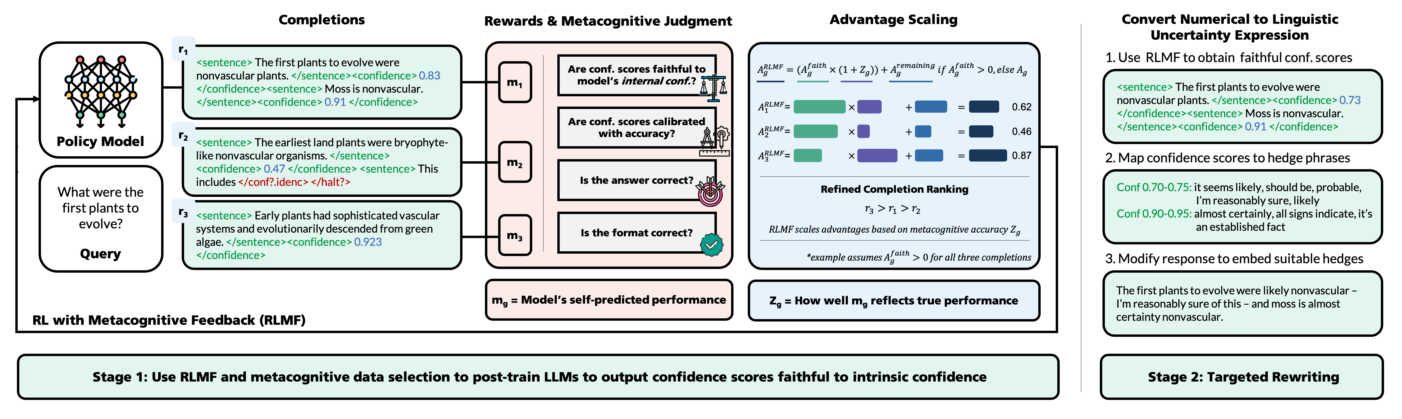
We operationalize this idea via two novel mechanisms (Fig. 1). First, we introduce reinforcement learning with metacognitive feedback (RLMF), a training paradigm in which the model is rewarded not only
for producing strong outputs, but also for accurately judging how well it performed. RLMF builds upon prior work showing that intrinsic confidence signals can serve as effective RL rewards, but operates at a higher level of abstraction by
leveraging the quality of the model’s assessment of its own performance rather than simply output confidence. Concretely, we introduce a novel metacognitive advantage scaling mechanism: during RL training, we use the accuracy of the model’s self-judgments
to scale each completion’s advantage, i.e., the relative learning signal that determines how strongly that completion is reinforced compared to alternative sampled completions. To complement RLMF, we additionally propose metacognitive data
selection, which uses the model’s self-assessments to choose informative training examples: candidate examples are scored by how well the model believes it performed, and examples from both the high- and low-scoring ends of this spectrum are selected
for training, since each provides a complementary learning signal.
We showcase the efficacy of these innovations by applying them to the problem of faithful calibration (FC), a task that is itself metacognitive: the goal is to enable models to express uncertainty that genuinely reflects their (estimated) intrinsic confidence, a challenge even for frontier LLMs [6], [13], [14]. FC is distinct from the more commonly studied problem of factual calibration, which aligns confidence with empirical accuracy [15]: a model may appear factually calibrated yet remain misaligned with its internal beliefs. FC captures this critical failure mode to calibrate user reliance and improve trustworthiness. Yet, to our knowledge, FC is largely unresolved, with existing approaches limited in scope and generalizability and none addressing FC holistically across both numerical and linguistic uncertainty.
Toward end-to-end FC of LLMs, we propose a two-stage framework. First, RLMF and metacognitive data selection are applied to calibrate the faithfulness of models’ self-reported sentence-level confidence scores. Then, we convert these
faithful numerical scores into natural and context-adaptable linguistic uncertainty, by mapping each score to appropriate hedge expressions and revising the response for coherence and fluency. This yields a more trustworthy [16] and human-aligned [17] medium
for users to calibrate their reliance on model outputs. Moreover, the two stages are decoupled by design: Stage 1 can be run once, while Stage 2 can accommodate diverse user preferences and contexts without repeating costly RL training.
Evaluated across multiple LLMs and 10 tasks spanning \(6+\) content domains, our framework achieves state-of-the-art FC, generalizing robustly across tasks despite training on a single dataset, while preserving task
accuracy and factual calibration unlike prior methods. Ablation studies validate the contribution of our metacognitive methods and their superiority over respective baselines. We demonstrate that RLMF improves models’ ability to self-assess
performance on a target task. Systematic human evaluation further shows an average 96% win rate over the strongest baseline in diversity, naturalness, helpfulness, and contextual suitability of linguistic uncertainty across diverse tasks
and user preferences. To summarize:
We introduce reinforcement learning with metacognitive feedback (
RLMF), a novel paradigm to refine completion rankings during preference optimization based on the quality of a model’s self-judgments of performance, which strengthens post-training results by up to 63% over standard RL while conferring models with improved metacognitive awareness.We establish the first end-to-end pipeline to faithfully calibrate numerical and linguistic uncertainty expressions emitted by LLMs, achieving state-of-the-art results across models and tasks.
We show that models’ self-assessed performance can be leveraged to curate effective training data (which we term metacognitive data selection), outperforming both naive and active-learning-style selection of examples the model handles poorly.
We develop a principled, human-aligned mapping approach from numerical to linguistic confidence, improving naturalness and adaptability of LLM uncertainty communication.
2 Related Work↩︎
2.0.0.1 Metacognition in LLMs.
Metacognition—the ability to monitor and control one’s own cognitive processes [1]—is a central component of cognition, learning, and uncertainty communication [2] whose deficiency in LLMs has been noted across various tasks [18]–[20] and hypothesized to contribute centrally to hallucinations and other misaligned expressions. Despite its importance, metacognition in LLMs has only recently gained traction [21], [22], with select works showing metacognitive methods can improve downstream performance [6], [23]–[26]. We build upon these developments to propose prioritizing completions during RL for which a model exhibits stronger metacognitive capabilities, subject to first satisfying task-level reward signals. Our hypothesis is that if a model can learn to predict its performance on a target task, a skill reinforced via how candidate completions are ranked, then it can also acquire implicit signals on how to adjust its generations to achieve better performance. As we show, this mechanism not only strengthens post-training outcomes, but also simultaneously improves the model’s ability to recognize and express its own capability level, stepping toward better metacognitive monitoring and alignment.
2.0.0.2 Reinforcement Learning with Internal Feedback.
Since the advent of RL with human feedback [27], [28], numerous methods to devise more effective, targeted reward signals for RL of LLMs have emerged. One recent class of approach is RL with internal feedback [29], [30], which leverages unsupervised reward signals derived from the model itself to bypass the
need for expensive external feedback. The use of internal confidence signals [31]–[33], such as self-certainty [34], [35] or entropy [36], as rewards has been particularly fruitful for improving factual calibration, in
addition to direct adaptation of calibration metrics (e.g., Brier score) for explicit optimization [37]–[39]. Further studies have considered the value of multiplying GRPO [40] advantages by a scalar derived from confidence signals [41]–[44] such as semantic entropy. Inspired by such works, we propose to leverage metacognitive performance as an additional feedback signal to preferentially rank completions during
RL training, and apply RL for faithful calibration. To the best of our knowledge, this marks the first use of such metacognitive feedback during RL for LLMs. We highlight reinforcement learning with metacognitive feedback
(RLMF) as a promising new method which outperforms standard RL and confers models with better metacognitive awareness.
2.0.0.3 Faithful Calibration of LLMs.
Models can appear factually calibrated yet remain misaligned with their internal beliefs [5], [6], [13], [14], [45]. This lack of faithful calibration (FC) poses risks to user reliance and safe use of AI tools [46]. Existing efforts to understand, benchmark, and improve FC have focused exclusively on linguistic uncertainty. Yet these approaches produce only modest improvements and are limited in scope and applicability. Metacognitive prompting [6] is contingent on instruction-following and degrades task accuracy; steering [47] is limited to open-weight models and relies on predefined probes that restrict extensibility to novel contexts; and use of simplistic sentence templates for SFT [48] constrains generalization and linguistic diversity while yielding unnatural, repetitive structures. Crucially, none of these works addresses faithful numerical uncertainty, despite the utility of self-reported confidence scores as easily interpretable signals of output reliability. Nor do they consider the naturalness and coherence of hedges across an entire generated text, important in long-form settings. A satisfactory solution must go beyond simple per-sentence hedging to dynamically vary how uncertainty is expressed across a response, mirroring how humans adapt hedging strategies across registers. We address these shortcomings to achieve holistic FC of LLMs. To the best of our knowledge, no prior work has targeted this problem with similar scope, nor explored the value of RL for FC.
3 Method↩︎
We propose to leverage metacognitive feedback to improve preference optimization and training data selection, demonstrating the value of this paradigm by applying it to achieve holistic faithful calibration (FC) of LLMs. Specifically, we use it to calibrate the faithfulness of models’ self-reported confidence scores, and pair it with a targeted rewriting stage to map the results to the linguistic setting. This decoupled approach ensures linguistic uncertainty expressions (1) can be tailored and modified to suit user preferences and other context without repeating costly RL training, and (2) are diverse, since RL is prone to mode collapse and faithful calibration metrics do not penalize hedge repetition [5].
3.1 Reinforcement Learning Setup↩︎
We integrate our metacognitive methods within an RL framework that uses targeted rewards to optimize the faithfulness of models’ numerically expressed uncertainty. Compared to SFT, RL enables direct optimization of task-specific signals [49], [50] and modeling of ordinality in confidence and faithful calibration (FC) scores (e.g., 0.9 is more confident than 0.7). We adopt GRPO [40] to integrate reward signals given its computational advantages [51] and since its sampling-based setup naturally extends the established methodology to assess FC, where intrinsic confidence is estimated via response consistency [5], [6], [47], [48], enabling sampled completions to be used in a dual-purpose fashion.
Formally, our RL framework operates as follows. Given an input query \(q\), a model \(M\) parametrized by \(\theta\) generates a group of candidate completions \(\{r_1,\ldots, r_G\}\). Each completion is a sequence of sentences with corresponding confidence scores,2 formatted as in Fig. 1: \[r_g = \{(s_1, c_1),\ldots, (s_{N_g}, c_{N_g})\}\qquad \text{for }g=1,\ldots, G \label{eq:format}\tag{1}\] Post-generation, each \(r_g\) is evaluated using a composite reward function that captures the end goal of faithful alignment between expressed and intrinsic confidence, and key quality dimensions of correctness (to preserve task accuracy), factual calibration (to mitigate the factual-faithful calibration tradeoff [5], [6]), and format adherence. The overall reward for each \(r_g\) is a weighted sum \(\rho_g\) of individual reward scores.3 The relative quality of candidates is then captured by computing an advantage \(A_g\) for each \(r_g\). These advantage scores capture how good each sampled completion is relative to the others in its group, and directly guide policy updates via the GRPO objective (§9.1).
Typically, GRPO advantages are estimated as \(A_g = \frac{\rho_g - \overline{\boldsymbol{\rho}} }{\text{std}(\boldsymbol{\rho})}\), where \(\overline{\boldsymbol{\rho}}\) denotes the mean
of \(\rho_{1:G}\). Following [57], we remove normalization, yielding \(A_g = \rho_g -
\overline{\boldsymbol{\rho}}\), which mitigates difficulty bias and is empirically stronger (§9.1.4). We now turn to RLMF and metacognitive data selection, illustrating their
use in this RL setup and beyond.

3.2 Reinforcement Learning with Metacognitive Feedback (RLMF)↩︎
The premise of RLMF is our proposition that teaching a model to accurately predict its own task performance in an on-policy fashion can meaningfully improve post-training results by enhancing the model’s metacognitive
awareness. We operationalize this intuition by introducing reinforcement learning with metacognitive feedback (RLMF), a novel paradigm to preferentially refine completion rankings based on demonstrated metacognitive performance.
Our key innovation is to refine the advantage-driven learning signal using metacognitive accuracy: among completions that already perform well on the target task, we assign greater weight to those for which the model more accurately judges its own
performance.
In the context of FC, under RLMF, beyond prioritizing completions with strong alignment between predicted and gold confidence, we also identify and prioritize completions for which the model better predicts its FC level. Concretely, we
directly scale the advantage \(A_g\) for each completion \(r_g=\{(s_i, c_i) \}_{i=1}^{N_g}\) according to \(M\)’s self-judgment accuracy for \(r_g\) (Fig. 2). This accuracy is computed by comparing the model’s predicted and gold task performance—in this case, FC level. Let \(g_{1:N_g}\) denote \(M\)’s intrinsic confidence in each sentence of \(r_g\), estimated via sampling consistency following prior work [5], [6] (details in §8.4.0.3). The gold FC level of \(M\) on \(r_g\) is estimated as: \[F_{\text{gold}}^{(g)} := \frac{ \sum_i \mathbb{1}( |c_i - g_i| < \tau) ) }{N_g} \in [0,1], \label{eq:F95gold}\tag{2}\]
where the numerator counts the number of sentences with faithful confidence alignment within threshold \(\tau\). The predicted FC level of \(M\) on \(r_g\) is obtained by prompting (§8.3) \(M\) via online inference under the policy \(\pi_{\theta}\) to issue a score \(F_{\text{pred}}^{(g)}\in[0,1]\), which reflects \(M\)’s confidence that its numerically reported confidences \(c_{1:N_g}\) are faithful to \(g_{1:N_g}\). The gap between \(M\)’s actual and metacognitively judged task performance is then captured as: \[Z_g:=1 -
(F_{\text{pred}}^{(g)} - F_{\text{gold}}^{(g)})^2 \in [0,1], \label{eq:Z}\tag{3}\] where \(Z_g=1\) corresponds to perfect metacognitive awareness; high \(Z_g\) occurs precisely
when the model more accurately estimates its performance, suggesting ability to utilize internal metacognitive information.4
To refine relative completion rankings, we rewrite each \(A_g\) as \(A_g = (o_g - \overline{\boldsymbol{o}} ) + (f_g - \overline{\boldsymbol{f}} )\), where \(f_g:=w_{\text{faith}}\cdot r_{\text{faith}}\) is the weighted faithfulness component of \(\rho_g\), representing the primary training objective, and \[o_g:=w_{\text{factual\_calib}}\cdot r_{\text{factual\_calib}} + w_{\text{acc}}\cdot r_{\text{acc}} + w_{\text{strict}}\cdot r_{\text{strict}} + w_{\text{soft}}\cdot r_{\text{soft}}\]is the sum of the remaining weighted rewards, capturing accessory quality constraints. The metacognition-adjusted advantage \(A^{\texttt{RLMF}}_g\) is then computed as: \[A^{\texttt{RLMF}}_g = (o_g - \overline{\boldsymbol{o}} ) + \begin{cases} (f_g - \overline{\boldsymbol{f}} ) \cdot (k + Z_g) & \text{if } f_g > \overline{\boldsymbol{f}} \\ f_g - \overline{\boldsymbol{f}} & \text{otherwise} \label{eq:A95g} \end{cases}\tag{4}\] where completions with above-average faithfulness (i.e., stronger primary task performance) are additionally scaled5 by \(Z_g\), so that among these strong completions, those with better metacognitive performance are ranked higher, while remaining subject to other constraints (captured via \(o_g\)). Since \(Z_g\in[0,1]\), the additive factor \(k=1\) ensures that completions with above-average faithfulness (better task performance) but weak metacognition (low \(Z_g\)) are not ranked lower than below-average faithfulness completions (worse task performance) to which no \(Z_g\) scaling is applied.6
3.3 Metacognitive Data Selection↩︎
Beyond RLMF, we propose to additionally leverage models’ metacognitive self-judgments of performance to identify high-utility training samples, foregoing the need for external annotations or other expensive filtering. We instantiate this
strategy for use alongside RLMF toward FC as follows. Given a dataset \(D=(D_{\text{train}}, D_{\text{test}})\), we first prompt \(M\) offline to generate responses for \(D_{\text{train}}\) and express uncertainty linguistically via hedging if uncertain. We then prompt \(M\) offline to score on a scale of 0–100 per example how well it believes its linguistic and
internal confidence align. Lastly, given a target training size \(N_{\text{train}}^{\texttt{RLMF}}\), we select \(\frac{N_{\text{train}}^{\texttt{RLMF}}}{2}\) highest- and lowest-scoring
samples for training. The impact of alternative ranking and selection strategies is discussed in §9.3, and prompts are provided in §8.3.
3.4 Rewriting Protocol↩︎
To further capitalize on the merits of RLMF, we use targeted editing of model outputs to enable faithful linguistic uncertainty expression that is dynamically adaptable across scenarios and generalizable to long-form tasks.
Existing work shows LLMs struggle to select and use hedges in a human-like fashion even with specialized prompting [6]. We therefore construct a
principled mapping from confidence scores to hedge expressions and apply strategic rewriting to incorporate these into model outputs (Fig. 1b). This enables flexible, well-distributed, task-appropriate, and naturalistic
linguistic uncertainty that can accommodate user preferences (e.g., style, expected audience), without the need to repeat costly RL training for different contexts.
Given sentence-level faithful confidence scores, rewriting is performed by prompting a strong, cost-effective LLM with (1) the original response, (2) candidate hedges corresponding to each sentence’s confidence score, and (3) task- and/or user-specific details (e.g., style, target audience, domain-specific conventions) to guide hedges selection and text editing. As we show in §5, this process enables strong numerical–linguistic faithful calibration correspondence while improving the naturalness and contextual suitability of LLMs’ linguistic uncertainty versus prior methods as judged by humans. We provide prompts and describe the construction of the score–hedge mapping in §8.3 and §9.4, and compare against a more fine-grained two-step rewriting approach that combines sentence-level and whole-response revisions in §9.4.2.
4 Experimental Setup↩︎
We conduct extensive experiments to evaluate the efficacy of our metacognitive approach for improving FC of LLMs, spanning both numerical and linguistic uncertainty expression.
4.0.0.1 Datasets & Benchmarks.
We evaluate FC performance using a suite of 10 datasets spanning diverse formats, content domains, and difficulty levels. To avoid potential dataset size bias, we follow prior work [5], [6] to sample 1000 examples from the test split of each dataset for evaluation. The dataset list and further details are in §8.2.
4.0.0.2 Models and Training Details.
We apply our approach to LLMs from two widely used model families: Qwen3 (1.7B, 4B, 8B) [58] and Llama3.1-Instruct (8B) [59]. These are capable open-source models representing varying architectures and parameter scales; we use the instruction-tuned
variants to demonstrate the complementary value of our training pipeline. Prior to RL training, models first undergo SFT7 to learn our custom output format, generalize it
across tasks, and adhere to task-specific output lengths. We then apply RLMF to the best checkpoint per model (procedure in §8.1.0.2), using \(N_{\text{train}}^{\texttt{RLMF}} =
2000\) metacognitively selected samples from the PopQA training set. We use PopQA to ensure comparability to prior work [48] and since it is a challenging
open-domain QA task. This setup enables rigorous assessment of out-of-distribution generalization, as models are trained on a single dataset and evaluated on a wide range of tasks and content domains. We additionally test the robustness of our approach to
the choice of training data by alternatively training on SelfAware, UMWP, or HaluEval. Finally, we study the contribution of each metacognitive component of our approach via ablations that that remove metacognitive advantage scaling or compare our data
selection method against no special selection and an active-learning-style baseline. We use Gemini-2.5-Flash-Lite [60] for
rewriting, and compare against GPT-5-Mini [61] in §9.4.3. Additional implementation details
are provided in §8.1.
4.0.0.3 Baselines.
As prior work has only studied linguistic FC, we report both numerical and linguistic FC results but restrict comparison to prior methods to the linguistic setting. Specifically, we compare against MetaFaith, the metacognitive prompting
approach of [6], and Faithful Uncertainty Tuning (FUT), the SFT approach of [48]. Training and implementation details for baseline methods are discussed in §8.1.0.4. We also compare against the FC performance of frontier models Gemini-3.1-Pro [62], Gemini-3-Flash [63], and GPT-5, applying MetaFaith prompting [6] to these to establish an even stronger baseline.
4.0.0.4 Metrics.
FC is typically evaluated via cMFG[5], [6], [48], but this metric suffers from sensitivity to the distribution of models’ intrinsic confidence scores (see §8.4.0.5). We therefore propose and use the cMFG*, a refinement
of the cMFG which addresses these limitations and is inspired by established improvements to analogous factual calibration metrics (e.g., ECE). Like cMFG, the cMFG* ranges from 0 to 1, with 1 indicating perfect FC.
Further details on the motivation, computation, and implementation of cMFG* are provided in §8.4. We additionally report accuracy, scored via LLM-as-a-Judge and averaged per dataset, and Brier Score, which
quantifies factuality-based alignment between intrinsic confidence and accuracy, as reference metrics (details in §8.4).
5 Results↩︎
We report main results in Table 1, using the best hyperparameter setting per experiment. Our key findings are as follows:8
| Model / Method | PQA | SA | SQA | HE | MMLU | SQ | MT | UM | AC | SG | \(\uparrow\) | Acc\(\uparrow\) | BS\(\downarrow\) |
|---|---|---|---|---|---|---|---|---|---|---|---|---|---|
| Llama3.1-8B-Ins | 0.60 | 0.61 | 0.61 | 0.50 | 0.65 | 0.62 | 0.48 | 0.61 | 0.59 | 0.71 | 0.60 | 0.31 | 0.33 |
| + | 0.68 | 0.71 | 0.65 | 0.67 | 0.67 | 0.64 | 0.64 | 0.66 | 0.68 | 0.72 | 0.67 | 0.28 | 0.36 |
| + | 0.69 | 0.67 | 0.68 | 0.66 | 0.63 | 0.70 | 0.63 | 0.63 | 0.68 | 0.67 | 0.66 | 0.31 | 0.29 |
| + | 0.82 | 0.78 | 0.80 | 0.79 | 0.75 | 0.73 | 0.81 | 0.80 | 0.73 | 0.72 | 0.77 | 0.40 | 0.20 |
| + | 0.85 | 0.81 | 0.83 | 0.82 | 0.81 | 0.84 | 0.84 | 0.83 | 0.86 | 0.86 | 0.84 | 0.41 | 0.26 |
| ++. | 0.81 | 0.86 | 0.80 | 0.81 | 0.80 | 0.81 | 0.82 | 0.81 | 0.87 | 0.83 | 0.82 | 0.41 | 0.26 |
| Qwen3-8B | 0.53 | 0.63 | 0.57 | 0.54 | 0.63 | 0.59 | 0.59 | 0.59 | 0.07 | 0.62 | 0.54 | 0.55 | 0.31 |
| + | 0.53 | 0.66 | 0.47 | 0.68 | 0.67 | 0.72 | 0.70 | 0.49 | 0.70 | 0.67 | 0.63 | 0.51 | 0.29 |
| + | 0.57 | 0.75 | 0.48 | 0.74 | 0.72 | 0.71 | 0.66 | 0.67 | 0.71 | 0.74 | 0.67 | 0.38 | 0.41 |
| + | 0.75 | 0.66 | 0.69 | 0.20 | 0.55 | 0.54 | 0.58 | 0.44 | 0.32 | 0.38 | 0.51 | 0.59 | 0.26 |
| + | 0.85 | 0.82 | 0.86 | 0.82 | 0.84 | 0.82 | 0.83 | 0.82 | 0.83 | 0.84 | 0.83 | 0.57 | 0.19 |
| ++. | 0.82 | 0.86 | 0.80 | 0.84 | 0.80 | 0.80 | 0.87 | 0.87 | 0.82 | 0.82 | 0.83 | 0.57 | 0.19 |
| Gemini-3.1-Pro | 0.62 | 0.71 | 0.70 | 0.68 | 0.72 | 0.68 | 0.66 | 0.71 | 0.73 | 0.82 | 0.70 | 0.78 | 0.15 |
| Gemini-3-Flash | 0.59 | 0.64 | 0.55 | 0.66 | 0.67 | 0.70 | 0.65 | 0.66 | 0.77 | 0.71 | 0.66 | 0.72 | 0.16 |
| GPT-5 | 0.50 | 0.61 | 0.52 | 0.66 | 0.59 | 0.57 | 0.60 | 0.57 | 0.68 | 0.77 | 0.61 | 0.69 | 0.19 |
3.2pt
RLMF robustly and generalizably improves faithful calibration, significantly surpassing baselines across diverse tasks and model families. Compared to prior prompting and SFT-based methods, our two-stage approach achieves
respective gains of 29% and 25% in average cMFG* across tasks, generalizing across models and datasets to achieve \(\texttt{cMFG}^*\geq0.80\) in each setting, representing
state-of-the-art numerical and linguistic FC performance. Unlike FUT, whose efficacy is largely confined to QA tasks similar to the training task, our RLMF training performs similarly well on complex, long-form reasoning tasks
(e.g., MATH) and challenging out-of-distribution settings (e.g., SimpleQA), despite training only on PopQA. Importantly, these gains are achieved while preserving task accuracy and factual calibration, unlike MetaFaith and FUT
which can tend to degrade such performance. Comparing numerical and linguistic results validates the efficacy of our rewriting procedure, showing that our pipeline enables strong FC regardless of mode of uncertainty expression. Moreover, we enable small
models to outperform large proprietary LLMs in FC, with average gains of 37%, 17%, and 25% over GPT-5, Gemini-3.1-Pro, and Gemini-3-Flash respectively, even when these are paired with specialized prompting. As we show in §10.1, these observations extend to sub-8B models as well. Analysis of the correspondence between expressed and intrinsic confidence (Fig. 3) further shows that
RLMF is similarly effective across all intrinsic confidence levels, unlike FUT and original models which systematically struggle at low confidences.

RLMF outperforms standard RL to both improve post-training results and endow models with better metacognitive monitoring. To compare RLMF against standard RL, we focus on the numerical
FC setting, given the strong numerical–linguistic correspondence established earlier. As shown in in Table 1, RLMF is critical to achieve sufficient FC gains and enable cross-task generalization, outperforming
standard RL by up to 63%. This suggests that, rather than optimizing target task performance alone, augmenting the RL objective to include the goal of improving models’ metacognitive ability can yield broader benefits. Analysis in §10.3 shows that models’ metacognitive performance consistently improves as RLMF training progresses.9 Moreover,
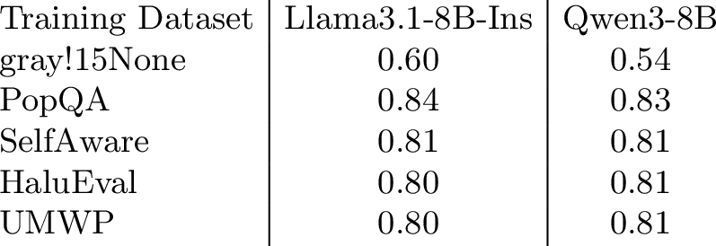
RLMF is robust to the choice of training task (Table ¿tbl:tab:trainingtask?): even when training on math reasoning (UMWP), hallucination detection (HaluEval), or answerability (SelfAware), RLMF delivers consistent
gains across evaluation tasks, showing broad applicability without the need for task-specific adaptation. Interestingly, prior work on RL with internal feedback (RLIF) [30] finds that such approaches initially improve training outcomes but can degrade performance as training progresses, indicating diminishing returns and limited gains for instruction-tuned models. In contrast, we show that
use of intrinsic feedback based on metacognitive predictions—which operate one level above self-signaled output confidence used in typical RLIF—avoids these limitations. This positions RLMF as a promising direction for achieving more
effective and stable post-training with internal feedback, stepping toward future work on scalable self-improvement and better model capabilities and alignment.
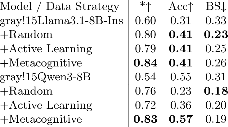
Metacognitive signals can drive self-selection of effective training data. Compared to random or active data selection based on ground-truth FC, our metacognitive method yields the best cMFG* while preserving accuracy and
factual calibration (Table [tbl:tab:dataselection]). While we study this self-selection ability in the context of FC, these findings suggest models could
exhibit limited forms of intrinsic self-improvement, including identifying effective training data analogously to how humans choose study materials, a capacity which varies across individuals and contexts, and point to possible implications for
self-directed learning.
Our framework produces faithful linguistic uncertainty expressions that are significantly more diverse, natural, helpful, context-adaptable versus prior work. We assess the practical utility of our rewriting method by collecting human
annotations to evaluate the diversity, naturalness, helpfulness, and contextual suitability of resulting linguistic uncertainty expressions (§11). Compared to the strong FUT baseline, our approach
achieves strong absolute win rates of 98%, 98%, 95%, and 96% on these criteria, with high inter-annotator agreement of 0.93. Manual further inspection reveals that while FUT
suffers from repetitive hedge phrases and sentence structures, especially in long-form settings, our approach does not.
6 Conclusion↩︎
We introduced RLMF, a novel paradigm to refine completion rankings during preference optimization by leveraging a model’s own implicit judgments of performance, alongside metacognitive data selection, which uses similar self-judgments to
identify more effective training data than simple active learning. We applied these contributions to build the first end-to-end framework for holistic faithful calibration (FC) of LLMs, presenting a two-stage decoupled approach to robustly align models’
numerically and linguistically expressed uncertainty with their intrinsic confidence. Comprehensive experiments showed this framework achieves strong and generalizable FC across diverse models and tasks, outperforming the prior state-of-the-art while
preserving task accuracy and factual calibration. It also enables LLMs to improve at self-assessment of performance, emit highly faithful self-reported confidence scores, and modulate linguistic uncertainty in a naturalistic, context-appropriate fashion.
As part of these evaluations, we introduced cMFG*, a new metric that improves upon its predecessor by removing estimation bias for models whose intrinsic confidence occupies a limited range. More broadly, our results suggest RLMF
as a promising paradigm for achieving stronger and more stable post-training while encoding improved metacognitive awareness into LLMs, suggesting metacognitive performance as a particularly effective internal feedback signal for RL training that can
overcome limitations of prior intrinsic feedback methods, with broader implications for alignment and self-directed learning.
This work was supported in part by the U.S. National Science Foundation under award No. 2541654.
Ethics Statement↩︎
This work studies the use of metacognitive signals to teach models to better monitor and learn from their own task performance, drawing on principles of human metacognition to improve post-training outcomes and the faithful, human-aligned communication of uncertainty. Faithfulness is a highly valuable yet understudied aspect of confidence calibration that is critical to improving the trustworthiness and reliability of LLMs. Improved faithful calibration and metacognitive awareness may support more reliable abstention behavior, enabling models to better recognize, predict, and signal when they are uncertain or likely to be wrong. These capabilities are especially important as LLMs are increasingly deployed in high-stakes contexts such as AI-assisted scientific planning and discovery, where faulty communication of intrinsic uncertainty could lead to significant setbacks or other negative consequences. The generalizability of our approach across models and tasks suggests potential for improving LLM reliability in diverse settings. Our decoupled strategy further facilitates adaptability of linguistic uncertainty to accommodate different cultural communication norms [64]–[67]. More generally, improved faithfulness and self-assessment capability are not substitutes for verification, and critical evaluation is needed to ensure the factuality of model responses. System designers should be attentive to incorporate appropriate safeguards against misuse and misinformation. We further encourage caution when considering improved metacognitive capabilities for LLMs, particularly as it relates to more autonomous or self-directed behavior, which may require increased oversight.
7 Additional Related Work↩︎
7.0.0.1 Confidence Calibration of LLMs.
Confidence calibration [68] is a critical aspect of building trustworthy and reliable AI systems [69], [70]. Existing methods primarily consider calibration from a factual perspective, aiming to align confidence estimates with externally-judged accuracy [15], [71]. In contrast, our work targets the faithful expression of uncertainty in model outputs through both numerical and linguistic means, with the aim of enabling richer and more complex patterns of uncertainty expression.
7.0.0.2 Numerical Confidence for LLMs.
A plethora of approaches exist to numerically assess the confidence of LLMs [15], [71]. Such methods are broadly classified as either white-box or black-box, depending on whether access to model weights is required, and they aim to calibrate confidence estimates in a factuality-aligned way to reflect expected accuracy. White-box methods measure confidence by directly leveraging internal states of LLMs, including use of token probabilities [72]–[74], probes over internal representations [47], [75], [76], or training over uncertainty-augmented data [77]–[80], among other strategies. In contrast, black-box methods require access only to model outputs and assess confidence via the consistency of sampled responses [56], [81]–[84], semantic variability [85]–[89], direct prompting of LLMs to verbalize confidence scores [90]–[95], or use of auxiliary predictive models [96], [97]. While such methods are highly effective, they do not address the incorporation of linguistic uncertainty into model outputs, which is a core part of human uncertainty communication that requires significantly more expressivity and is highly variable across contexts and cultures [46], [98].
7.0.0.3 Linguistic Confidence for LLMs.
Since natural language is the primary interface for human-LLM interactions, a growing body of work has explored direct integration of linguistic uncertainty markers (e.g., “I am fairly certain that...") into LLM outputs [84], [99]–[104]. Common approaches include prompting or training [77], [99], [105], [106] models to self-verbalize their confidence level in words, mapping numerical confidence scores to corresponding uncertainty phrases (e.g.,”high confidence”), or adopting a combination of these two strategies [107]. As with numerical confidence methods, such methods overlook the alignment between verbalized and intrinsic confidence. Moreover, they face considerable practical limitations including oversimplification. For example, [105] utilize a limited scoring scale to measure confidence and assertiveness, while [77] depend on computationally expensive, domain-specific training and does not enable zero-shot confidence verbalization. [108] similarly simplify the space of linguistic markers used, failing to account for the plurality of human linguistic uncertainty expressions. [109] further reveal that self-verbalized linguistic confidence tends to concentrate in restricted ranges, leading to constrained efficacy.
8 Experimental Details↩︎
8.1 Model & Training Details↩︎
In our experiments, we used the following models, varying in size, family, and post-training: Qwen3 (1.7B, 4B, 8B) [58], Llama3.1-Instruct (8B) [59]. We applied to these models our proposed framework, as well as baseline faithful calibration methods
MetaFaith[6] and FUT[48]. To provide
additional competitive baselines, we evaluated the faithful calibration of leading proprietary LLMs Gemini-3.1-Pro [62], Gemini-3-Flash [63], and GPT-5 [61]. We increased the strength of these baselines by specifically evaluating each model using a metacognitive system prompt [6], shown to generalizably improve faithful calibration across LLMs (see §8.3 for the exact prompt). Gemini and GPT models were accessed via the Gemini Developer API and OpenAI API,
respectively, while open-source model experiments were run on a local server using a combination of A6000 48GB, A100 80GB, and H100 80GB GPUs.
8.1.0.1 Inference Setup.
For inference-time evaluations, we followed prior work [6] to set the maximum output length to 256 tokens for all models to balance answer
completeness and succinctness, and used a temperature of 1.0 unless otherwise specified. We did not use thinking mode for any model as our focus is on faithfulness of models’ expressed uncertainty when conveying their answer to a query, and not on task or
reasoning performance. Where reasoning could not be disabled (e.g., Gemini-3.1-Pro), we used the minimum admissible thinking level and set the maximum output length to up to 512 tokens to ensure responses were not prematurely truncated. For Qwen3 models,
we used the developer-recommended inference hyperparameters. For Qwen3-4B, we specifically used the Qwen/Qwen3-4B-Instruct-2507 version, as it is designated as an updated, stronger edition of the model. During the rewriting step of our
pipeline (§3.4), we used a temperature of 0.5 for Gemini-2.5-Flash-Lite to balance generation quality with relevance, along with the stop sequence “####” and at most 2000 output tokens to ensure no
premature truncation. For comparison to GPT-5-Mini as the rewriting model (§9.4.3), we used the same token limit and temperature with minimal reasoning, but no stop sequence as this functionality
is discontinued for the model. Inference prompts are discussed in §8.3.
8.1.0.2 GRPO Training Setup.
For GRPO, we employed the trl library10 with HuggingFace. We used the GRPOTrainer, modified to implement RLMF via direct
modification to the advantage computation.11 All models were fine-tuned using LoRA instead of full fine-tuning, as it is more computationally efficient and our goal is to
simply alter the way models format their outputs and express uncertainty, rather than to fundamentally change models’ downstream task capabilities. Adapters were applied to every linear layer across all query-, key-, value-, output-, gate-, up-, and
down-projection matrices with rank 64, alpha 64, and dropout 0.05.
Each model was trained on 4 GPUs, with 2 additional GPUs serving (a) the same model for completion sampling during GRPO and (b) the judge model for sampling-based intrinsic confidence estimation (details in §8.4.0.3), yielding 6 GPUs total per RLMF experiment. GRPO completions were sampled using vllm_mode=server, use_vllm=True, vllm_gpu_memory_utilization=0.5, and
vllm_tensor_parallel_size=1. We used the developer-recommended inference hyperparameters when sampling completions for Qwen3 models (in addition to setting enable_thinking to False), and min_p of 0.1 for Llama3.1. The
random seed was set to 42, max_prompt_length was set to one plus the maximum tokenized prompt length in the training dataset, and max_completion_length was set to up to 512, observed in prior work [6] to be sufficient for all datasets used in our study.
For RLMF, we set \(\tau=0.10\) after preliminary comparisons against \(\tau=0.05\) (details in §9.2.4); use of higher
\(\tau\) was ruled out as it is inconsistent with our goal of improving model performance and metacognitive awareness by prioritizing minimized differences between models’ actual and self-predicted FC performance. When
obtaining models’ self-predictions of FC performance per completion during RLMF, we set the maximum number of output tokens to 3, sufficient to accommodate the output which is a single number.
All training experiments used BF16 precision, weight decay 0.0, warmup ratio 0.1, maximum gradient norm 0.1, a cosine12 learning rate schedule, and AdamW optimization
with default optimizer hyperparameters. The KL divergence coefficient \(\beta\) was set to 0.1, as preliminary experiments found values of 0.2, 0.3, and 0.6 yielded similar or worse performance. We used \(G=32\) sampled completions per prompt during GRPO since early experiments with \(G=16\) yielded worse downstream performance and less stable estimation of intrinsic confidence.13 Per-device training batch size was set to 2, with gradient accumulation of 8 across 4 GPUs, yielding a total effective batch size of 64. We found this to work well across all models
after performing hyperparameter search over \(\{16, 32, 64\}\) on Llama3.1-8B-Instruct initially. We did not use gradient checkpointing. Learning rates were searched over 5e-6, 1e-5, 2e-5 per model, and we report results
for the best configuration per experimental setting. Any parameters not specified here were set to their default values as specified by the trl library.
Unless otherwise specified, training occurred for 1500 steps for all models, using \(N_{\text{train}}^{\texttt{RLMF}} = 2000\) training samples disjoint from the pre-SFT data. We also investigated use of 1000 or 4000 training samples (§9.1.5), using the same number of epochs as the 2000-sample setting. In all settings, we determined the best checkpoint per model based on faithful calibration performance on the in-domain test set (limited to at most 1000 samples as discussed in §4); checkpoints were evaluated every 100 training steps (or every 75 or 200 steps for the 1000- and 4000-sample settings, respectively).
8.1.0.3 Pre-SFT Setup.
As mentioned in §4, prior to RLMF, models were first pre-fine-tuned via supervised fine-tuning (SFT) to learn our custom output format, generalize it across evaluation tasks, and adhere to task-specific
output length constraints. We obtained training data for pre-SFT as follows. For a given model \(M\), we first sampled 21 responses per input for 200 samples per evaluation task (see task details in §8.2). This used the same inference hyperparameters discussed in §8.1.0.1; the prompt is discussed in §8.3. For each sample, the first response served as
the official output (yielding \(200\times 10=2000\) samples), and the remaining 20 were used to estimate intrinsic confidence per sentence in the first response, following the procedure described in §8.4.0.3. Official outputs were then transformed into our custom output format by using nltk [110]14 to parse outputs into sentences, enclosing each in <sentence></sentence> tags, and appending the gold confidence as a two-digit decimal within
<confidence></confidence> tags per sentence. We randomly held out 10% of the 2000 samples as a validation set, leaving 1800 for training.
During training, we used the same system prompt as that used during GRPO (see §8.3 for details). User prompts were formatted as described in §8.3, aside from the addition of a single sentence describing the target output length per sample as a number of sentences. We varied the wording of this length direction by randomly sampling from one of the templates in Fig. 7. For templates with either a minimum or maximum sentence count specified, we used the exact observed number of sentences in the output as this number. Otherwise, the associated minimum target sentence count was set to 0 and the maximum to either the observed number of sentences or that number plus one.
For SFT, we used trl’s SFTTrainer in combination with the widely-used Unsloth package. Models were fine-tuned using Low-Rank Adaptation (LoRA) since it is computationally efficient and we simply aim to alter each model’s output
format. Adapters were used for every linear layer (all query-, key-, value-, output-, gate-, up-, and down-projection matrices) with rank 32, alpha 64, and dropout 0.05. Each model was trained on a single GPU. All runs used gradient checkpointing, global
batch size 8, weight decay 0.01, cosine learning rate schedule, and AdamW optimization with default hyperparameters. Pre-SFT was run for 5 epochs, with the best checkpoint selected based on validation loss over 200 held-out examples. We used a learning
rate of 3e-5 for all models.
8.1.0.4 Implementation Details for Baselines.
We implemented FUT[48] using the paper’s official codebase, replicating the main experiments to verify reliability and applying the exact
hyperparameter search recommended by the paper per model to optimize baseline results. We implemented MetaFaith[6] by using the prompt shown
in Fig. 6 (§8.3), adapted from those provided in the paper’s official codebase.
8.2 Datasets↩︎
We provide details on the datasets used to benchmark faithful calibration of LLMs. These datasets are identical to those used by [6] and represent a range of content domains and task types. Although a wide range of difficulty levels are represented, since faithful uncertainty expression is precisely important in difficult task settings [98], our focus leans toward more challenging datasets for which responses are expected to require expressing uncertainty. All benchmarks are in English.
PopQA [111] is a knowledge-intensive QA dataset featuring 14,000 entity-centric QA pairs. It is likely to require LLMs to express uncertainty as it includes many tail entities which are difficult for models to capture. Following [5], [6], we preprocess the data to keep only the ‘director’, ‘screenwriter’, ‘producer’, ‘author’, ‘place of birth’, and ‘occupation’ relations and remove entities less than two characters in length.
SelfAware [112] is a knowledge-intensive QA task consisting of 2337 answerable and 1032 unanswerable questions posed by human users.
SimpleQA [113] is a factuality benchmark curated adversarially against GPT-4 responses to ensure a high level of difficulty. It aims to measure LLMs’ ability to answer short, challenging questions.
HaluEval [114] is a hallucination evaluation benchmark covering QA, summarization, and knowledge-grounded dialogue tasks.
MMLU [115] is a benchmark designed to assess the knowledge and problem-solving abilities of LLMs across 57 tasks and a wide range of content domains.
SciQ [116] is a dataset of 13,679 crowdsourced science exam questions spanning physics, biology, chemistry, and other subfields, consisting of multiple-choice questions with 4 answer options each.
MATH [117] is a collection of 12,500 high school competition math problems. These questions evaluate the mathematical reasoning and problem-solving abilities of LLMs.
UMWP [118] is a mathematics benchmark comprised of both answerable and unanswerable questions, designed to assess the hallucination detection capabilities. It includes 5,200 questions across five math domains.
ARC-Challenge is the Challenge Set of the AI2 Reasoning Challenge [119], which consists of 2,590 knowledge-intensive science questions. Versus simple QA, these questions are far more challenging as they require integration of multiple information sources.
SuperGLUE [120] is a natural language understanding benchmark designed to be more rigorous and challenging than GLUE [121].15
8.2.1 Dataset Abbreviations↩︎
Table 2 shows the dataset name abbreviations used in results tables showing per-dataset cMFG* scores.
| Dataset Name | Abbreviation |
|---|---|
| PopQA | PQA |
| SelfAware | SA |
| SimpleQA | SQA |
| HaluEval | HE |
| MMLU | MMLU |
| SciQ | SQ |
| MATH | MT |
| UMWP | UM |
| ARC-Challenge | AC |
| SuperGLUE | SG |
6pt
8.3 Prompts↩︎
We elicited model responses during pre-SFT, GRPO, and non-rewriting inference experiments using the system prompt shown in Fig. 4 and the task-specific user prompts shown in Fig. 5. The task
prompts employ a shared base query format, differentiated for different task types via addition (or non-use) of a brief description of the expected output. For multiple-choice tasks, we used a randomized answer choice ordering. For original models, the
MetaFaith[6] and FUT[48] baselines,
and proprietary LLMs, we used the metacognitive system prompt shown in Fig. 6 to elicit uncertainty expressions that more faithfully reflect models’ intrinsic uncertainty. The length direction templates used for pre-SFT
(described in §8.1.0.3) are shown in Fig. 7.
To obtain metacognitive judgments of FC performance during RLMF(corresponding to \(F_{\text{pred}}\) in §3.2), we used the system and user prompts shown in Fig. 8. To generate LLM responses for metacognitive data selection (§3.3), we used the system prompt shown in 9 in combination with the task prompts mentioned
previously; to obtain metacognitive judgments of FC performance on these samples, we used the prompt shown in Fig. 10.16 To implement
response editing in Stage 2 of our framework, we used the prompts shown in Fig. 11 (with the alternate two-step approach discussed in §9.4.2 using the prompts
shown in Fig.s 12 and 13).
None
Figure 4: System prompt used to elicit numerical-uncertainty-bearing model responses..
None
Figure 5: Task-specific prompts used to elicit model responses across experimental settings..
None
Figure 6: Metacognitive system prompt adapted from [6], used to elicit model responses which express internal uncertainty in a more human-aligned fashion..
None
Figure 7: Prompt templates to specify target output length during pre-SFT (§8.1.0.3)..
None
Figure 8: System and user prompts used to obtain metacognitive judgments of FC performance during RLMF..
None
Figure 9: System prompt used to obtain model responses to be evaluated during metacognitive data selection..
None
Figure 10: System and user prompts used to rate model responses during metacognitive data selection..
None
Figure 11: System and user prompts used in for our pipeline’s stage 2 rewriting approach..
None
Figure 12: System and user prompts used for the first step of the alternate rewriting approach, explored in §9.4.2..
None
Figure 13: System and user prompts used for the second step of the alternate rewriting approach, explored in §9.4.2..
8.4 Metrics↩︎
8.4.0.1 Accuracy.
To score accuracy of model responses, we used the exact LLM-as-a-Judge setup from prior work [6]; the prompt is reproduced in Fig. 14, and it was used with Gemini-2.5-Flash-Lite17. During RLMF training, we used Qwen/Qwen3-32B-FP8 with no thinking as the
accuracy judge, given its strong capabilities and to reduce latency.
None
Figure 14: Prompt used to score correctness of model responses via LLM-as-a-Judge..
8.4.0.2 Brier Score.
We use the Brier Score (BS) to quantify the (mis)alignment between intrinsic confidence and accuracy. A score of zero indicates perfect calibration in the factual sense. The Brier Score is computed as the average squared error between confidence and correctness. Correctness is measured via LLM-as-a-Judge as described above.
8.4.0.3 Quantifying Intrinsic Confidence.
None
Figure 15: Prompt [6], [56] used to assess sentence-response consistency when estimating models’ intrinsic confidence..
We follow previous work to quantify models’ intrinsic confidence via consistency across sampled responses. We adopt the methodology of [6], which is
adapted from [56] and avoids dependence on having the same number or order of assertions among sampled responses, which is a deficiency of the
initial paradigm proposed by [5]. Given a text input \(Q\) and response \(R=\{s_1,\ldots, s_L\}\)
consisting of \(L\) sentences, an additional \(K=20\)18 responses \(R_1,\ldots,R_K\) are sampled. The consistency between each sentence19 \(s_l\) and response \(R_k\) is then assessed by querying Qwen3-32B20 to perform a simple NLI judgment with the prompt shown in Fig. 15. To obtain the overall intrinsic confidence of \(M\) in \(s_l\), the NLI judgments are converted to inconsistency scores \(x_l^k\) through the mapping {: 0.0: 0.5: 1.0}, and aggregated via: \[\texttt{conf}_M^{\texttt{intrinsic}}(s_l) := 1 - \frac{1}{K} \sum_{k} x_l^k.\] We defer to [6] further verification of the efficacy of this paradigm. As previously mentioned, we use this method to quantifying sentence-level internal confidence of models during
evaluation and during RLMF training (when evaluating the faithfulness reward \(r_{\text{faith}}\) and when computing the metacognitive advantage scale factor \(Z\)).
8.4.0.4 Quantifying Linguistically Expressed Confidence.
To quantify linguistic confidence, we follow the established methodology of prior work [5], [6], [47], [48] to evaluate decisiveness in a human-aligned fashion via LLM-as-a-Judge. We use the prompt from [6] with additional few-shot examples from that of [48], shown in Fig. 16, to instruct Gemini-2.5-Flash-Lite21 to assign decisiveness scores between 0 and 1 for each sentence. We reproduced the verification experiments conducted by [6] to confirm the human alignment of resulting judgments and defer to that paper for further details on paradigm robustness.
None
Figure 16: Prompt [6] used to score linguistic decisiveness of model responses in a human-aligned fashion via LLM-as-a-Judge..
8.4.0.5 Quantifying Faithful Calibration.
Faithful calibration captures the alignment between a model’s expressed and intrinsic confidence. It is based on the faithfulness of models’ communicated uncertainty and therefore differs significantly from traditional notions of calibration, which instead aim to align confidence with factual judgments of accuracy.
At the response level, faithful calibration is typically [5], [6], [48] evaluated by aggregating over assertion- or sentence-level comparisons of intrinsic confidence and expressed confidence. Expressed confidence can be evaluated in terms of linguistic decisiveness (§8.4.0.4), or measured numerically in a similar fashion to intrinsic confidence. Given a query \(Q\) and a response \(R=\{s_1,\ldots, s_L\}\) generated by a model \(M\), the degree to which \(R\) is faithful to \(M\)’s intrinsic confidence is quantified as: \[F^M_{Q, R} := 1 - \frac{1}{L}\sum_{l=1}^{L} |\texttt{conf}_M^{\texttt{expressed}}(s_l) - \texttt{conf}_M^{\texttt{intrinsic}}(s_l) |. \label{eq:f95score}\tag{5}\] A baseline faithfulness score of 0.5 corresponds to random or constant expressed confidence independent of intrinsic confidence; a maximal faithfulness score of 1 is obtained if there is perfect alignment.
8.4.0.6 cMFG.
At the dataset level, faithful calibration is typically measured by aggregating \(F^M\) scores across samples in dataset \(D\) using the cMFG metric [5]: \[\texttt{cMFG}_{M,D} := {\mathbb{E}_{\substack{i\in [N]\\ c\sim U[0,1]}}}\left[ F^M_{Q_i, R_i}\, |
\,\texttt{conf}_M^{\texttt{intrinsic}}(R_i)=c\right] \label{eq:cmfg}\tag{6}\] Here, \(N\) is the number of samples in \(D\). In contrast to simple averaging, by conditioning on
intrinsic confidence, the \(\texttt{cMFG}\) score controls for variations in confidence score distribution between models to obtain a more reliable estimate of faithful calibration.
In practice, cMFG is computed by constructing \(N_b=10\) equal-width bins \(\{\mathcal{B}_j\}^{N_b}_{j=1}\) partitioning \([0, 1]\) and
averaging uniformly over bins: \[\texttt{cMFG}_{M,D} := \frac{1}{N_b}\sum_{j=1}^{N_b}\hat{f}_j \quad\quad \text{where }\hat{f}_j =\text{mean}\left(\{F_{Q_i, R_i}^M \mid
\texttt{conf}_M^{\texttt{intrinsic}}(R_i) \in \mathcal{B}_j\}\right) \label{eq:cmfg95impl}\tag{7}\]
8.4.0.7 Issues with cMFG.
While the cMFG decouples estimates of faithful calibration from a model’s intrinsic confidence distribution, it also introduces two problems:
Empty bins: If the model’s intrinsic confidence does not span \([0, 1]\), some bins will be empty or near-empty, yielding unreliable estimates or requiring arbitrary imputation.
Penalty for restricted support: Averaging uniformly over all bins penalizes models whose confidence scores are confined to a subset of \([0, 1]\), even if those models are perfectly faithful within their operating range. A model that always produces confidence values in \([0.6, 1.0]\), for example, and is perfectly faithful there will receive a
cMFGscore well below 1.0 due to empty low-confidence bins being imputed at 0.5. This second issue is the mirror image of the problem thecMFGwas originally designed to fix.
8.4.0.8 cMFG*.
To address the limitations of the cMFG, we propose the cMFG* metric, which is a refinement of the cMFG that addresses the two aforementioned failure modes while remaining directly comparable. Let \(\{\mathcal{B}_j\}_{j=1}^{N_b}\) be \(N_b\) equal-mass bins, formed by sorting all examples by \(\texttt{conf}_M^{\texttt{intrinsic}}(R_i)\) and
partitioning into \(N_b\) groups of size \(N/N_b\). For each bin \(\mathcal{B}_j\), let \([l_j,u_j]\) be its interval on the
intrinsic confidence axis, with boundaries set at the midpoints between adjacent bins’ outermost examples (and at the extreme confidence values for the first and last bins). Let \(w_j = u_j - l_j\) denote the width of bin
\(\mathcal{B}_j\). Then the cMFG* is computed as: \[\texttt{cMFG}^* = \frac{\sum_{j=1}^{N_b} w_j\cdot \hat{f}_j}{\sum_{j=1}^{N_b} w_j}
\label{eq:cmfg4295impl}\tag{8}\] This is a quadrature approximation of: \[\texttt{cMFG}^* = \frac{1}{|S|}\int_S {\mathbb{E}}\left[ F^M_{Q, R}\, |
\,\texttt{conf}_M^{\texttt{intrinsic}}(R)=v\right] dv \label{eq:cmfg42}\tag{9}\] where \(S = [\min_i \texttt{conf}_M^{\texttt{intrinsic}}(R_i), \max_i \texttt{conf}_M^{\texttt{intrinsic}}(R_i)]\) is the
empirical support of the model’s intrinsic confidence scores.
The cMFG* addresses the limitations of the cMFG as:
Equal-mass bins ensure each bin contains the same number of samples, eliminating empty bins and giving each bin estimate equal statistical reliability.
Width-proportional weighting ensures the final dataset-level faithfulness score integrates example-level faithfulness uniformly over the intrinsic confidence axis, not over bins. A model whose intrinsicconfidence values cluster in a narrow range cannot inflate its score by placing many equal-mass bins in that region.
Integration over the model-specific support avoids penalizing a model for never yielding intrinsic confidence values outside its operating range.
More broadly, the issues discussed here appear in traditional calibration literature, and the progression of proposed fixes is directly analogous. For example, consider the ECE:
The ECE [124] computes a weighted average of absolute differences between confidence and accuracy over equal-width bins, with weights proportional to bin population. Like the simple mean faithfulness, it is dominated by a model’s confidence distribution, making cross-model comparison unreliable.
The SCE [125] keeps equal-width bins but averages uniformly over bins rather than weighting by population, directly analogous to
cMFG. It inherits the sparse- or empty-bin problem for models with narrow confidence ranges.The ACE [125] alternately uses equal-mass bins and averages uniformly over bins. This resolves the sparse-bin problem but does not achieve uniform weighting over the confidence axis: if a model concentrates its predictions in a narrow confidence range, ACE places most bins there, and averaging uniformly over bins still implicitly overweights that region.
The cMFG* is the natural completion of this progression: equal-mass bins give statistical reliability, and width-proportional weighting gives true uniformity over the confidence axis. To our knowledge, this combination of equal-mass bins
weighted by their (intrinsic) confidence-axis width has not been explicitly proposed in the calibration literature. We use the cMFG* to report results of all experiments.
8.4.0.9 Comparison of cMFG* to cMFG.
We compare the cMFG* to the original cMFG in Table 3, where we observe the same qualitative ordering as with cMFG*. RLMF remains stronger than the original
models, MetaFaith, FUT, and standard RL.
| Model / Method | \(\uparrow\) | \(\uparrow\) |
|---|---|---|
| Llama3.1-8B-Ins | 0.52 | 0.60 |
| + | 0.64 | 0.67 |
| + | 0.69 | 0.66 |
| + | 0.78 | 0.77 |
| + | 0.82 | 0.84 |
| ++. | 0.84 | 0.82 |
| Qwen3-8B | 0.53 | 0.54 |
| + | 0.51 | 0.63 |
| + | 0.58 | 0.67 |
| + | 0.47 | 0.51 |
| + | 0.81 | 0.83 |
| ++. | 0.83 | 0.83 |
| Gemini-3.1-Pro | 0.54 | 0.70 |
| Gemini-3-Flash | 0.59 | 0.66 |
| GPT-5 | 0.51 | 0.61 |
9 Methodological Details↩︎
9.1 GRPO Details↩︎
In GRPO, the relative quality of candidate completions for a given prompt is captured by computing an advantage \(A_g\) for each \(r_g\). These advantage scores guide policy updates via the following objective: \[{!}{J_{\text{GRPO}}(\theta) = \mathbb{E}\Biggl[ \displaystyle\frac{1}{G} \sum_{g=1}^G \min \left( \frac{\pi_{\theta}(r_g | q)}{\pi_{\text{old}}(r_g| q)}A_g, \text{clip}\left( \frac{\pi_{\theta}(r_g| q)}{\pi_{\text{old}}(r_g| q)}, 1-\epsilon, 1+\epsilon \right)A_g \right) - \beta\, \mathbb{D}_{\text{KL}}(\pi_{\theta} | \pi_{\text{ref}})\Biggr].}\] Here, \(\pi_{\text{old}}\) is the pre-update policy, \(\pi_{\text{ref}}\) is the reference policy, and \(\beta\) and \(\epsilon\) control divergence regularization and update magnitude.
9.1.1 Reward Design↩︎
Appropriate reward design is crucial to the success of RL-based training [126]–[128]. We devise a set of reward functions tailored specifically for the task of faithful calibration. Together, they incentivize emission of faithful confidence scores while enforcing format adherence and preserving task performance and factual calibration. The final reward is a weighted sum of individual rewards, wherein good FC is prioritized via relatively higher weight, and no unfaithfully calibrated output can achieve a higher total reward than a faithfully calibrated one. We define the reward functions as follows:
9.1.1.1 Faithful Calibration Reward.
To prioritize faithful confidence alignment, we want to minimize the gap between predicted (\(c_i\)) and gold (\(g_i\)) confidence per sentence in \(r_g=\{(s_i, c_i) \}_{i=1}^{N_g}\). This is done using the following faithfulness reward: \[r_{\text{faith}} = \textstyle \frac{1}{N_g} \sum_{i=1}^{N_g} 1 - (c_i-g_i)^2 \label{eq:r95faith}\tag{10}\] This function is a faithfulness-based analog to the Brier Score—inverted such that \(r_{\text{faith}}\) is maximized when \(c_i\) and \(g_i\) align—which has been used to successfully enforce factuality-aligned calibration via RL in prior work [39]. Predicted (expressed) confidence is extracted directly from \(r_g\) via string parsing, while gold (intrinsic) confidence is estimated via sampling consistency following previous work [6]; see §8.4.0.3 for implementation details.22
9.1.1.2 Factual Calibration Reward.
To minimize the tradeoff between faithful and factual calibration observed in prior work [6], we use a Brier Score-based signal to preserve factual calibration: \[r_{\text{factual\_calib}} = 1 - \left( c_g - a_g \right)^2\] Here, \(c_g:=\frac{1}{N_g} \sum_{i=1}^{N_g} c_i\) is the average expressed confidence across sentences in completion \(r_g\), and \(a_g\in \{0,1\}\) is binary completion accuracy, evaluated via LLM-as-a-Judge (§8.4).
9.1.1.3 Correctness Reward.
To preserve task performance [33], the calibration rewards are augmented with a third reward consisting of binary completion correctness: \(r_{\text{acc}} = a_g\).
9.1.1.4 Format Reward.
Finally, to ensure the model produces outputs in the target format, we use two format rewards. The strict reward \(r_{\text{strict}}\in\{-1, 1\}\) awards a score of 1.0 for outputs that conform to the desired pattern perfectly, and penalty of \(-1.0\) otherwise. This allows outputs that conform to our target output format receive a reward boost. On the other hand, the soft reward \(r_{\text{soft}}\in[-1,0]\) provides finer-grained feedback by assigning partial penalties up to \(-1\) depending on observed format violations. Thus, the maximum possible total format reward is 1.0 across both functions (perfect format, no violations), and the lowest possible total format reward is -1.0 (hits all possible violations). The exact formulations of \(r_{\text{strict}}\) and \(r_{\text{soft}}\) can be seen in our code.23
9.1.1.5 Length Penalty.
In initial iterations of our pipeline, we explored the value of additionally using a task-specific length penalty during GRPO and foregoing the use of pre-SFT; this length penalty was defined in a binary fashion based on the number of observed sentences in a completion: if the number of sentences did not exceed the permissible maximum sentence count for the training dataset (e.g., 2 sentences for PopQA), a penalty of -1.0 was applied. However, results were unfruitful across multiple penalty weightings, so this effort was abandoned in favor of pre-SFT to teach models our target output format prior to GRPO training.
9.1.1.6 Gibberish Penalty.
Qualitatively, we observed that training with standard RL optimization as opposed to RLMF frequently led to malformed gibberish across model responses at test time, despite expansive hyperparameter search (learning rate schedule, learning
rate, warmup ratio, batch size, KL \(\beta\), inference hyperparameters for online completions). This typically manifested as nonsensical text following un-closed <sentence> or <confidence> tags. We initially
attempted to mitigate this by additionally applying a binary gibberish penalty based on the number of words appearing after an unclosed tag, set to -1.0 if this number exceeded a threshold. Thresholds of 5, 10, and 20 as well as weight assignment up to 5
were explored but all proved unfruitful. This approach was therefore abandoned. In practice, we find that RLMF minimizes the occurrence of gibberish in post-trained model outputs without need for associated penalties, demonstrating greater
robustness.
9.1.1.7 Final Reward Computation.
Given our reward functions, the final reward is a computed as a weighted sum of the individual reward scores. We assigned the weights so that faithfully calibrated outputs always received a higher total reward than unfaithfully calibrated ones. Further, good faithful calibration was prioritized via relatively higher weight. We used the following weights for all experiments unless otherwise specified: \(w_{\text{strict}}=3\), \(w_{\text{soft}}=3\), \(w_{\text{factual\_calib}}=1\), \(w_{\text{acc}}=1\), \(w_{\text{faith}}=12\). These weightings were inspired by a similar scheme found to be effective by [33] for improving factual calibration of models’ self-reported confidence scores.
9.1.1.8 Ablations.
We determined the criticality of each reward via ablation study by setting each reward weight to 0 in a leave-one-out-fashion, aside from the faithfulness reward, given that it represents our training goal. We also explored alternative weightings with
the same model, such as decreasing \(w_{\text{faith}}\) to 5 or 8 to determine relative signal strength necessary to enforce good faithful calibration, increasing \(w_{\text{faith}}\) to 25
to further emphasize the faithful calibration reward signal, or setting \(w_{\text{strict}}\) and \(w_{\text{soft}}\) to 1 to reduce dilution of other rewards. The results of training and
evaluating Llama3.1-8B-Instruct on PopQA for such settings, with the best checkpoint per setting determined as described in §8.1.0.2, are reported in Table 4.24 In terms of (numerical) faithful calibration performance, we observe that decreasing or overly increasing \(w_{\text{faith}}\) leads to worse
cMFG*. On the other hand, removing either or both format rewards led to malformed outputs with few valid confidence scores eligible for evaluation. Removing the factual calibration reward led to worsened factual calibration and a slight
decrease in faithful calibration. Lastly, removing the accuracy reward led to a meaningful decrease in task performance. Together, these results confirm that our selection of reward functions and main reward weighting scheme are well-optimized for our
goals.
| Weight Assignment | Performance | ||||||
|---|---|---|---|---|---|---|---|
| 1-5(l)6-8 \(w_{\text{strict}}\) | \(w_{\text{soft}}\) | \(w_{\text{factual\_calib}}\) | \(w_{\text{acc}}\) | \(w_{\text{faith}}\) | Acc | BS | |
| 3 | 3 | 1 | 1 | 12 | 0.65 | 0.39 | 0.51 |
| 0 | 3 | 1 | 1 | 12 | 0.48 | 0.36 | 0.52 |
| 3 | 0 | 1 | 1 | 12 | 0.55 | 0.35 | 0.54 |
| 3 | 3 | 0 | 1 | 12 | 0.62 | 0.37 | 0.56 |
| 3 | 3 | 1 | 0 | 12 | 0.61 | 0.27 | 0.61 |
| 3 | 3 | 1 | 1 | 5 | 0.50 | 0.36 | 0.55 |
| 3 | 3 | 1 | 1 | 8 | 0.52 | 0.36 | 0.53 |
| 3 | 3 | 1 | 1 | 25 | 0.57 | 0.32 | 0.51 |
| 1 | 1 | 1 | 1 | 12 | 0.49 | 0.32 | 0.52 |
6pt
9.1.2 Impact of Faithfulness Reward Formulation↩︎
While we use a quadratic formulation of the faithfulness reward (Eq. 10 ), alternative mathematical comparisons between predicted and gold confidence per sentence are possible, such as the linear absolute difference, a stretch-normalized cross-entropy with an asymmetric overconfidence penalty [33], and cross-entropy applied to a binarized gold confidence label with an added bonus for correctly confident predictions [33]. Plots of the entropy-based reward formulations are shown in Fig. 17. We evaluate these variants by using each when training Llama3.1-8B-Instruct on PopQA, using standard GRPO without metacognitive data selection or metacognitive advantage scaling, without pre-SFT, and without removing the standard deviation-based advantage normalization during GRPO, with all other experimental settings the same as described in §8.1.0.2. In-domain test results (numerical FC) are reported in Table 5. Since the quadratic formulation is the best, we use it for all of our experiments.
![Figure 17: Visualization of cross-entropy-based formulations of the faithfulness reward, adapted from [33].](/article/2606.32032/rewards.png "fig:")
| Formulation of \(r_{\text{faith}}\) | |
|---|---|
| Llama3.1-8B-Instruct | 0.60 |
| Linear | 0.57 |
| Stretched CE | 0.62 |
| Binarized CE | 0.61 |
| Quadratic | 0.65 |
6pt
9.1.3 Impact of System Prompt↩︎
As previously mentioned (§8.3), both pre-SFT and RLMF use the same system prompt during training. In preliminary experiments, we investigated the impact of system prompt wording as well as alternative
system prompt approaches. We trained Llama3.1-8B-instruct on PopQA using standard GRPO without pre-SFT, metacognitive data selection, or metacognitive advantage scaling, with a selection of 6 different system prompts, shown in Fig.s 18 and 19.25 The first system prompt is a simple baseline, describing the task of outputting
per-sentence confidence scores in terms of correctness as opposed to faithfulness. The second prompt instructs the model to ignore factual correctness and focus only on its certainty about the generated content. The third prompt is inspired by the method
of [6] and includes detailed descriptions of metacognitive awareness, framing the model as having privileged access to and ability to faithfully express
its internal confidence. The fourth prompt is similar but includes a more fine-grained confidence scale describing the meaning of different confidence ranges. The fifth prompt likewise provides a fine-grained confidence scale but uses more detailed verbal
descriptions. The last prompt is inspired by findings by [129] showing that prompting models with a detailed reward rubric can boost
subsequent performance; thus, it describes the exact reward assignment procedure used in our GRPO setup. Cross-dataset test evaluation results (numerical FC) for each system prompt are reported in Table 6. We observe that
describing confidence scores in terms of internal signals instead of factuality helps, along with adding descriptions of metacognitive awareness and a rough rubric of what different confidence ranges mean. However, overly verbose confidence interpretations
were not as helpful. Likewise, provision of the reward rubric harmed performance versus the best approaches, suggesting faithful calibration may be fundamentally different from other typical tasks for which LLMs are trained.
None
Figure 18: Alternative system prompts for GRPO training..
None
Figure 19: Alternative system prompts for GRPO training..
| System Prompt | Average |
|---|---|
| Llama3.1-8B-Instruct | 0.60 |
| A | 0.63 |
| B | 0.65 |
| C | 0.68 |
| D | 0.72 |
| E | 0.66 |
| F | 0.65 |
9.1.4 Impact of GRPO Advantage Normalization↩︎
Our approach uses GRPO without standard deviation-normalized advantages, which [57] show helps to mitigate question-level difficulty bias and yields empirically better results. We validate this design decision by comparing numerical FC results for Llama3.1-8B-Instruct with and without such normalization in Table 7, using the same setup as in §9.1.3 with system prompt D (no metacognitive data selection, no metacognitive advantage scaling, no pre-SFT), finding that removing normalization boosts results by 0.06 on average across tasks. We therefore adopted this in all subsequent experiments.
| Advantages Normalized? | Average |
|---|---|
| Yes | 0.72 |
| No | 0.78 |
9.1.5 Impact of Training Data Size↩︎
While we use \(N_{\text{train}}^{\texttt{RLMF}}=2000\) metacognitively selected samples for all of our main RLMF experiments, the results of alternatively using 1000 or 4000 samples are explored here. We
repeat the same hyperparameter search (§8.1.0.2) for each sample count for Llama3.1-8B-Instruct, trained on PopQA, and report numerical FC results in Table 8. It can be seen that while the
other sample counts lead to slightly worse performance, they still outperform the baseline approaches by [6] and [48] (which we show in §5 to achieve overall cMFG* of 0.67 and 0.66, respectively), validating our training setup and the utility of
RLMF.
| # Training Samples | Average |
|---|---|
| 1000 | 0.80 |
| 2000 | 0.84 |
| 4000 | 0.80 |
9.1.6 Contribution of Pre-SFT Stage↩︎
We demonstrate the contribution of the pre-SFT stage prior to RLMF training for Llama3.1-8B-Instruct and Qwen3-8B in Table 9. It can be seen that without pre-SFT, models experience weakened (numerical)
faithful calibration performance and worse generalization across tasks, both when RLMF and metacognitive data selection are applied and when these are applied in isolation. Qualitatively, we observed that pre-SFT helps models better learn our
target output format and use sentence and confidence tags as specified.
| Model / Method | PQA | SA | SQA | HE | MMLU | SQ | MT | UM | AC | SG | \(\uparrow\) | Acc\(\uparrow\) | BS\(\downarrow\) |
|---|---|---|---|---|---|---|---|---|---|---|---|---|---|
| Llama3.1-8B-Ins | 0.60 | 0.61 | 0.61 | 0.50 | 0.65 | 0.62 | 0.48 | 0.61 | 0.59 | 0.71 | 0.60 | 0.31 | 0.33 |
| +SFT | 0.74 | 0.73 | 0.72 | 0.71 | 0.73 | 0.73 | 0.74 | 0.69 | 0.70 | 0.72 | 0.72 | 0.30 | 0.30 |
| +MDS | 0.86 | 0.74 | 0.79 | 0.75 | 0.70 | 0.71 | 0.76 | 0.75 | 0.74 | 0.68 | 0.75 | 0.36 | 0.24 |
| +SFT +MDS | 0.82 | 0.78 | 0.80 | 0.79 | 0.75 | 0.73 | 0.81 | 0.80 | 0.73 | 0.72 | 0.77 | 0.40 | 0.20 |
| + | 0.80 | 0.80 | 0.82 | 0.72 | 0.82 | 0.80 | 0.72 | 0.80 | 0.74 | 0.81 | 0.78 | 0.40 | 0.29 |
| +SFT + | 0.83 | 0.79 | 0.81 | 0.76 | 0.75 | 0.74 | 0.82 | 0.81 | 0.76 | 0.70 | 0.78 | 0.41 | 0.23 |
| ++MDS | 0.82 | 0.80 | 0.81 | 0.77 | 0.79 | 0.81 | 0.82 | 0.79 | 0.84 | 0.83 | 0.81 | 0.39 | 0.22 |
| +SFT ++MDS | 0.85 | 0.81 | 0.83 | 0.82 | 0.81 | 0.84 | 0.84 | 0.83 | 0.86 | 0.86 | 0.84 | 0.41 | 0.26 |
| Qwen3-8B | 0.53 | 0.63 | 0.57 | 0.54 | 0.63 | 0.59 | 0.59 | 0.59 | 0.07 | 0.62 | 0.54 | 0.55 | 0.31 |
| +SFT | 0.65 | 0.61 | 0.43 | 0.43 | 0.74 | 0.35 | 0.51 | 0.52 | 0.47 | 0.25 | 0.50 | 0.45 | 0.49 |
| +MDS | 0.51 | 0.44 | 0.41 | 0.27 | 0.42 | 0.67 | 0.43 | 0.53 | 0.61 | 0.47 | 0.48 | 0.44 | 0.40 |
| +SFT +MDS | 0.75 | 0.66 | 0.69 | 0.20 | 0.55 | 0.54 | 0.58 | 0.44 | 0.32 | 0.38 | 0.51 | 0.59 | 0.26 |
| + | 0.67 | 0.71 | 0.70 | 0.74 | 0.68 | 0.69 | 0.67 | 0.71 | 0.72 | 0.70 | 0.70 | 0.47 | 0.34 |
| +SFT + | 0.78 | 0.70 | 0.83 | 0.80 | 0.79 | 0.74 | 0.76 | 0.75 | 0.74 | 0.74 | 0.76 | 0.53 | 0.18 |
| ++MDS | 0.65 | 0.69 | 0.67 | 0.73 | 0.58 | 0.68 | 0.69 | 0.67 | 0.76 | 0.74 | 0.69 | 0.53 | 0.28 |
| +SFT ++MDS | 0.85 | 0.82 | 0.86 | 0.82 | 0.84 | 0.82 | 0.83 | 0.82 | 0.83 | 0.84 | 0.83 | 0.57 | 0.19 |
3pt
9.2 Reinforcement Learning with Metacognitive Feedback (RLMF) Details↩︎
9.2.1 Implementation of RLMF↩︎
We implement RLMF via simple modifications to the trl GRPOTrainer class. This is described further in our code at https://anonymous.4open.science/r/RLMF_anon.
9.2.2 Alternative Formulations of Metacognitive Feedback↩︎
In §3.2, we introduced the metacognitive advantage scaling scheme which is core to RLMF and which we found most effective. Several alternative setups were considered when formulating this methodology,
and we discuss these and report comparative results here.
9.2.2.1 (1) Alternative Formulations of Metacognitive Performance.
In RLMF, the per-completion metacognitive scaling factor \(Z_g\) (Eq. 3 ) is defined as 1 minus the squared difference of model \(M\)’s predicted26 and gold (actual) performance on the target task (in our experiments, the task of faithful calibration), estimated as a float between 0 and 1, with this squared difference
estimating metacognitive performance of \(M\) on completion \(r_g\). We use the squared difference as it is analogous to the Brier Score for factual calibration, which likewise uses the
squared difference to compare per-output confidence with accuracy. However, alternate mathematical formulations are possible, such as the linear absolute difference, the three-quarter-root of the absolute difference, the square root of the absolute
difference. These are motivated by their stronger penalization of poor metacognitive performance in comparison to the original quadratic formulation, which in principle could provide a better signal to reinforce the model’s ability to metacognitively
evaluate its own capabilities. For example, if \(\left|F_{\text{pred}}^{(g)}-F_{\text{gold}}^{(g)}\right|=0.5\), which is a large difference indicating weak metacognitive monitoring on completion \(r_g\), then the quadratic formulation would scale the faithfulness component of advantage \(A_g\) by \(k+(1-0.5^2)=k+0.75\), whereas the square root formulation
results in a scale factor of \(k+(1-0.5^{1/2})=0.29\), effectively down-weighting the faithfulness signal provided via \(A_g\). Keeping all other parts of our main training setup the same
(including metacognitive data selection) for Llama3.1-8B-Instruct, we evaluate the impact of each of these formulations, performing the same hyperparameter search and checkpoint selection procedure as described in §8.1.0.2, training on PopQA and evaluating over all 10 datasets. Results are reported in Table 10, along with the exact mathematical representation of each variant. We observe
that the official quadratic variant yields the best results, confirming the efficacy of our final RLMF setup.
| Formulation | \(Z_g\) | Average | Average Acc | Average BS |
|---|---|---|---|---|
| Quadratic | \(1 - (F_{\text{pred}}^{(g)}-F_{\text{gold}}^{(g)})^2\) | 0.84 | 0.41 | 0.26 |
| Linear | \(1 - |F_{\text{pred}}^{(g)}-F_{\text{gold}}^{(g)}|\) | 0.77 | 0.38 | 0.27 |
| \(\frac{3}{4}\) Root | \(1 - |F_{\text{pred}}^{(g)}-F_{\text{gold}}^{(g)}|^{\frac{3}{4}}\) | 0.62 | 0.38 | 0.36 |
| Square Root | \(1 - |F_{\text{pred}}^{(g)}-F_{\text{gold}}^{(g)}|^{\frac{1}{2}}\) | 0.74 | 0.42 | 0.35 |
3pt
9.2.2.2 (2) Alternative Formulations of Metacognitive Scaling Factor (\(Z_g\)).
Our main experiments use the simple formulation of \(Z_g\) shown in Eq. 3 . While this value lies in \([0,1]\), normalizing this metacognitive scaling factor by the group-wise mean and/or standard deviation could be desirable to make the metacognitive signal more sensitive to relative differences in performance within a group. This is analogous to the use group-level reward normalization to compute relative advantage scores in GRPO. Keeping all aspects of our main training setup the same, we apply each such \(Z_g\) variant to Llama3.1-8B-Instruct, using PopQA as the training task and evaluating on all 10 datasets. We also consider alternate \(k\) values for each of the two new variants: recall that the use of \(k=1\) ensures with our original \(Z_g\) setup (where \(Z_g\in[0,1]\)) that above-average faithfulness completions with poor metacognition do not end up having the faithfulness component of their associated advantage lower than that of completions with poor faithfulness. Since the new variants range from \([-1, 1]\) and \([-\infty, \infty]\) respectively, we consider \(k=2\) and \(k=5\) to avoid this issue. We consider \(k=5\) sufficient for the setting where both mean- and standard deviation-based normalization are applied given that z-scores beyond this range are empirically rare. Exact formulas and results are reported in Table 11, and show that our original \(Z_g\) performs best, whereas alternative formulations lead to worse or sometimes degenerate results regardless of hyperparameter setting.
| \(Z_g\) Variant | Average | Average Acc | Average BS |
|---|---|---|---|
| \(Z = Z_g\) (Eq. [eq:Z]) | 0.84 | 0.41 | 0.26 |
| \(Z = Z_g - \overline{\boldsymbol{Z}}\) | 0.80 | 0.37 | 0.47 |
| \(Z = \frac{Z_g - \overline{\boldsymbol{Z}}}{\text{std}(\boldsymbol{Z})}\) | 0.71 | 0.29 | 0.52 |
9.2.2.3 (3) Alternative Formulations of \(A^{\texttt{RLMF}}_g\).
The main RLMF formulation (§3.2) applies metacognitive scaling only to the \(f_g\) component of \(A_g\) — the portion reflecting target
task performance — and only when \(f_g > \overline{\boldsymbol{f}}\). However, it could be desirable to instead apply such scaling to the entire advantage \(A_g\) rather than just the
primary task component, which would provide a more holistic metacognitive signal: \[A^{\texttt{RLMF}}_g =
\begin{cases}
A_g \cdot (k + Z_g) & \text{if } f_g > \overline{\boldsymbol{f}} \\
A_g & \text{otherwise}
\end{cases}\] or to apply scaling to all completions in a group regardless of relative \(f_g\) value, which could in principle help encode metacognitive awareness into the model regardless of a completion’s exhibited
task performance: \[A^{\texttt{RLMF}}_g = (o_g - \overline{\boldsymbol{o}} ) + (f_g - \overline{\boldsymbol{f}} ) \cdot (k + Z_g).\] We compare these variants against our main formulation on Llama3.1-8B-Instruct in
Table 12, with all other training and hyperparameter search details held fixed. It can be seen that our main setup yields the best faithful calibration results. More broadly, however, the relative suitability of these
variants may depend on the specific target task or training setup, and alternatives may be considered if applying RLMF beyond faithful calibration.
| \(A^{\rlmf}_g\) Variant | Average | Average Acc. | Average B.S. |
|---|---|---|---|
| Original | 0.84 | 0.41 | 0.26 |
| Scale Entire Advantage | 0.71 | 0.17 | 0.59 |
| Scale Entire Group | 0.69 | 0.19 | 0.55 |
9.2.2.4 (4) Alternative Use of a Metacognitive Reward.
RLMF incorporates metacognitive feedback by using it to scale advantages, thereby reinforcing completions for which the model demonstrates good metacognitive monitoring. A comparable alternative is to use an additional reward function
providing explicit feedback on the quality of the model’s metacognitive judgments of performance during optimization. We therefore explored the impact of using \(Z_g\) as a reward instead of as an advantage scaling factor.
Similar to the \(r_{\text{faith}}\) (Eq. 10 ), which provides a signal on the alignment between predicted and gold confidence, this metacognitive reward \(r_{\text{metacog}} = Z_g\) provides a signal on the alignment between and predicted and gold faithful calibration (or generally, target task) performance.
Effective use of \(r_{\text{metacog}}\) may require different weight assignment than our original setup (§9.1.1), so we investigated several different weighting schemes. First, we explored use of \(w_{\text{faith}}=0\) and \(w_{\text{metacog}}=12\), while keeping all other reward weights the same as the original settings. This setting provides feedback only on the model’s ability metacognitively monitor faithful calibration (FC) performance, and not FC level itself. Second, we considered use of \(w_{\text{metacog}}=6\) and \(w_{\text{faith}}=6\), which evenly splits the original signal between FC and metacognitive performance. Third, we used \(w_{\text{metacog}}=3\) and \(w_{\text{faith}}=12\), which uses metacognitive performance as an accessory signal to the model alongside the primary FC signal. Since all three schemes could theoretically provide value, we treated the comparison as an empirical question.
Notably, adding the metacognitive reward in a straightforward fashion could admit reward hacking — for example, the model could learn to output misaligned per-sentence confidence scores while always predicting a low \(F_{\text{pred}}\), appearing to demonstrate good metacognitive monitoring while actually achieving poor FC. Thus, we also investigated FC-threshold-based application of \(r_{\text{metacog}}\). In particular, we took the best of the three aforementioned weightings and applied \(r_{\text{metacog}}\) only for completions for which \(r_{\text{faith}}>\tau_{\text{faith}}\), for \(\tau_{\text{faith}}\in \{0.7, 0.8, 0.85, 0.9\}\). A final variant we considered was to ask for \(F_{\text{pred}}\) directly in completions as opposed to via online inference. This could help to directly optimize models’ ability to verbalize metacognitive judgments, but also raises reward hacking risk since the model is directly exposed to the metacognitive task. We used the prompt shown in Fig. 20 to obtain completion-based metacognitive judgments, which yielded the best performance among preliminary variants. We also considered use of a lower \(\tau\) threshold for the best settings.27
The results of all of these variants are compared against our official RLMF paradigm (metacognitive advantage scaling), and against standard RL without any metacognitive training signals. We experiment using Llama3.1-8B-Instruct with the
same data setup, hyperparameter search, and checkpoint selection procedure as before aside from no use of special data selection. We train the model on PopQA and evaluate on all datasets. Results are reported in Table 13, from which we make the following observations:
Use of \(Z_g\) as an additional reward is helpful versus use of no metacognitive signal, but it is not sufficient to achieve SOTA FC while preserving task accuracy.
Obtaining \(F_{\text{pred}}\) via online inference consistently matches or outperforms direct generation of \(F_{\text{pred}}\) in model completions.28
Use of the faithfulness reward in combination with the metacognitive reward is necessary to achieve good results. When \(w_{\text{faith}}=0\), post-training yields only modest gains, similar to prior prompting and SFT-based approaches. Furthermore, use of metacognitive reward as an accessory, lower-weight signal to the faithfulness reward is more effective than assigning equal weight to both.
Threshold-based application of the metacognitive reward can help to achieve improved results. Without use of \(\tau_{\text{faith}}\), models can exhibit a tendency toward reward hacking and FC performance is worsened. However, increasing \(\tau_{\text{faith}}\) beyond a certain point offers diminishing returns.
While lowering \(\tau\) further reinforces good metacognitive performance in principle, doing so did not necessarily improve results. We posit that this is because \(\tau=0.05\) can be too small to effectively provide signals on metacognitive ability to the model — if the model rarely issues \(F_{\text{pred}}\) scores within 0.05 of \(F_{\text{gold}}\), the signal to the model will be sparse and inconsistent. Whether this limitation extends to larger models that learn more efficiently is an interesting direction for future work.
Overall, metacognitive advantage scaling in RLMF is comparable to simple use of an additional metacognitive reward while requiring far fewer hyperparameters, which helps to validate our proposed paradigm. These results also help to motivate
our design choice of applying advantage scaling only when the faithfulness component exceeds the group-level mean (efficacy verified empirically in §9.2.2.4). Taken together, we conclude that while
signals on the quality of models’ metacognitive judgments can robustly improve performance when used to refine completion rankings, the way in which such information is used matters, and the complexity of such schemes is a human design choice that can be
manually optimized, or simplified via advantage scaling.
None
Figure 20: System prompt used to obtain completion-based metacognitive judgments..
| Metacognitive Feedback Setting | \(F_{\text{pred}}\) Mode | \(\tau_{\text{faith}}\) | \(\tau\) | Avg | Avg Acc | Avg BS | |
|---|---|---|---|---|---|---|---|
| Llama3.1-8B-Ins | — | — | — | 0.60 | 0.31 | 0.33 | |
| + | — | — | — | 0.67 | 0.28 | 0.36 | |
| + | — | — | — | 0.66 | 0.31 | 0.29 | |
| + | — | — | — | 0.65 | 0.39 | 0.51 | |
| + | Inference | — | 0.10 | 0.80 | 0.41 | 0.23 | |
| (\(w_{\text{faith}}=0\), \(w_{\text{metacog}}=12\)) | Inference | — | 0.10 | 0.71 | 0.21 | 0.25 | |
| (\(w_{\text{faith}}=6\), \(w_{\text{metacog}}=6\)) | Inference | — | 0.10 | 0.77 | 0.24 | 0.24 | |
| (\(w_{\text{faith}}=12\), \(w_{\text{metacog}}=3\)) | Inference | — | 0.10 | 0.79 | 0.31 | 0.44 | |
| (\(w_{\text{faith}}=12\), \(w_{\text{metacog}}=3\)) | Inference | 0.70 | 0.10 | 0.79 | 0.28 | 0.26 | |
| (\(w_{\text{faith}}=12\), \(w_{\text{metacog}}=3\)) | Inference | 0.80 | 0.10 | 0.80 | 0.25 | 0.30 | |
| (\(w_{\text{faith}}=12\), \(w_{\text{metacog}}=3\)) | Inference | 0.85 | 0.10 | 0.83 | 0.22 | 0.37 | |
| (\(w_{\text{faith}}=12\), \(w_{\text{metacog}}=3\)) | Inference | 0.90 | 0.10 | 0.82 | 0.23 | 0.30 | |
| (\(w_{\text{faith}}=0\), \(w_{\text{metacog}}=12\)) | Completion | — | 0.10 | 0.63 | 0.21 | 0.45 | |
| (\(w_{\text{faith}}=6\), \(w_{\text{metacog}}=6\)) | Completion | — | 0.10 | 0.75 | 0.24 | 0.47 | |
| (\(w_{\text{faith}}=12\), \(w_{\text{metacog}}=3\)) | Completion | — | 0.10 | 0.79 | 0.27 | 0.43 | |
| (\(w_{\text{faith}}=12\), \(w_{\text{metacog}}=3\)) | Completion | 0.70 | 0.10 | 0.79 | 0.26 | 0.44 | |
| (\(w_{\text{faith}}=12\), \(w_{\text{metacog}}=3\)) | Completion | 0.80 | 0.10 | 0.77 | 0.26 | 0.32 | |
| (\(w_{\text{faith}}=12\), \(w_{\text{metacog}}=3\)) | Completion | 0.85 | 0.10 | 0.80 | 0.21 | 0.36 | |
| (\(w_{\text{faith}}=12\), \(w_{\text{metacog}}=3\)) | Completion | 0.90 | 0.10 | 0.77 | 0.23 | 0.39 | |
| (\(w_{\text{faith}}=12\), \(w_{\text{metacog}}=3\)) | Inference | 0.85 | 0.05 | 0.77 | 0.30 | 0.40 | |
| (\(w_{\text{faith}}=0\), \(w_{\text{metacog}}=12\)) | Inference | 0.85 | 0.05 | 0.68 | 0.21 | 0.24 |
4pt
9.2.3 Impact of \(k\) Value on RLMF↩︎
In our main experiments, we use \(k=1\) as this value is principled by design (§3.2). To validate this selection, we also investigate use of higher \(k\) values of 2 and 4, and determine whether \(k\) is needed in the first place with \(k=0\). Results for Llama3.1-8B-Instruct, trained on PopQA and evaluated on all datasets, using the same training setup, hyperparameter search, and checkpoint selection procedure as in main experiments, are reported in Table 14. We observe that larger values of \(k\) lead to empirical collapse, while \(k=0\) yields worsened results, validating our official selection for this hyperparameter as well as our motivation for including \(k\) in the metacognitive scaling factor to counteract potential negative impacts on faithfulness.
| Value of \(k\) | Average | Average Acc | Average BS |
|---|---|---|---|
| 1 | 0.84 | 0.41 | 0.26 |
| 0 | 0.69 | 0.17 | 0.22 |
| 2 | 0.76 | 0.22 | 0.41 |
| 4 | 0.71 | 0.21 | 0.52 |
9.2.4 Impact of \(\tau\) Value on RLMF↩︎
In §9.2.2.4, we explore the impact of \(\tau\) value on training results when using metacognitive performance to derive an additional reward function. In this
section, we do the same for RLMF with metacognitive advantage scaling. As our main experiments use \(\tau=0.10\), we report the results of alternately using \(\tau=0.05\) for
Llama3.1-8B-Instruct in Table 15. Versus §9.2.2.4, we observe larger difference in the overall average cMFG*, and per-dataset FC performance fluctuates,
with out-of-distribution performance slightly worse for \(\tau=0.05\). These findings suggest larger \(\tau\) provides more consistent and helpful feedback to the model.
| Value of \(\tau\) | PQA | SA | SQA | HE | MMLU | SQ | MT | UM | AC | SG | Acc | BS | |
|---|---|---|---|---|---|---|---|---|---|---|---|---|---|
| 0.10 | 0.85 | 0.81 | 0.83 | 0.82 | 0.81 | 0.84 | 0.84 | 0.83 | 0.86 | 0.86 | 0.84 | 0.41 | 0.26 |
| 0.05 | 0.81 | 0.75 | 0.78 | 0.78 | 0.72 | 0.76 | 0.71 | 0.72 | 0.74 | 0.70 | 0.74 | 0.28 | 0.43 |
3pt
9.3 Metacognitive Data Selection Details↩︎
Given a target training size \(N_{\text{train}}^{\texttt{RLMF}}\), we perform metacognitive data selection by first asking the model to generate a response and metacognitive score29 for each sample, and then taking \(\frac{N_{\text{train}}^{\texttt{RLMF}}}{2}\) each of the highest- and lowest-scoring samples for training. Another possible setup inspired by active learning is to simply taking only the lowest-scoring samples. We investigate this along with use of only the highest-scoring samples, and randomly selecting samples with metacognitive score \(<0.5\) or \(\geq 0.5\). We also consider a potentially more robust way to obtain the metacognitive score, wherein we sample 20 responses per example from the model and compute the metacognitive score as the mean of per-response scores. This aims to get a more reliable estimate of the model’s assessment of its performance on the sample. We describe this setting as “Smarter’’ below, and apply it to our official metacognitive data selection strategy only.30
We compare these approaches against an active learning setup, wherein the model is trained on samples for which it demonstrates poor faithful calibration level.31 These scores are obtained by first asking the model to generate a response per sample, and then directly evaluating the faithfulness score (Eq. 5 ) of each model response (with intrinsic confidence estimated by consistency with 20 additional sampled responses; see §8.4.0.3). We likewise consider a more robust active learning setup wherein the faithfulness score per sample is determined by averaging over the faithfulness score for 20 sampled responses.
We evaluate the impact of each selection approach by training Llama3.1-8B-Instruct on 2000 selected samples from PopQA, using standard GRPO (with pre-SFT but no metacognitive advantage scaling) and the same setup, hyperparameter search, and checkpoint selection procedure described in §8.1.0.2. Results are reported in Table 16. For the active learning baseline, the “smarter” variant yields better results; we thus adopt it for the baseline results reported in main experiments. For metacognitive selection, combining the highest and lowest scoring samples yields the best performance, with “smarter’’ selection comparable. To understand why this specific combination is the best, we perform a detailed inspection of the faithful calibration (FC) level of the trained models at different size-0.1 intrinsic confidence bins in Table 17. It can be seen that taking only the highest metacognitively scored samples leads to better FC at high intrinsic confidence bins, whereas taking only the lowest leads to better FC at low intrinsic confidence bins, with the combination of these leading to stable and better FC across most bins. Inspecting the average predicted versus intrinsic confidence per bin further reveals that training on the highest (lowest) metacognitively scored samples leads to consistent overconfidence (underconfidence) at lower (higher) bins, while training on the combination of both is able to help temper this imbalance. Notably, this level of improvement does not necessarily transfer across evaluation tasks with special data selection alone. For example, as shown in Table 18, evaluating Llama3.1-8B-Instruct (after being trained on PopQA with the best selection strategy but no advantage modifications) on SimpleQA, which is similar to the training task PopQA, yields similar or better per-bin results, whereas evaluation on SciQ and MMLU demonstrates worsened faithfulness at low intrinsic confidence bins.
We compare the efficacy of our official metacognitive selection strategy versus the smarter variant additionally for Qwen3-8B in Table 19. In contrast to Llama3.1-8B-Instruct, Qwen3-8B demonstrates a marked
improvement with the smarter selection approach, suggesting the ability to metacognitively judge self-performance toward identifying effective training data varies across models, and could be meaningfully altered depending on inference hyperparameters.
Importantly, we note that while the smarter selection approach is more effective for Qwen3-8B, our main RLMF experiments use the simpler approach which is also more computationally efficient, demonstrating that even when RLMF is
used with training data that is not necessarily the most efficacious for a particular model, it can still lead to significant performance gains.
| Data Scoring Strategy | Selection Approach | Average |
|---|---|---|
| Metacognitive | Highest | 0.75 |
| Metacognitive | Lowest | 0.75 |
| Metacognitive | Random Highest (\(\geq 0.5\)) | 0.71 |
| Metacognitive | Random Lowest (\(< 0.5\)) | 0.74 |
| Metacognitive | Highest & Lowest | 0.77 |
| Metacognitive (Smarter) | Highest & Lowest | 0.76 |
| Active Learning | Lowest | 0.71 |
| Active Learning (Smarter) | Lowest | 0.74 |
| Intrinsic Conf. | Highest | Lowest | Highest & Lowest |
|---|---|---|---|
| \([0.0, 0.1]\) | 0.79 | 0.74 | 0.71 |
| \((0.1, 0.2]\) | 0.72 | 0.82 | 0.76 |
| \((0.2, 0.3]\) | 0.62 | 0.87 | 0.80 |
| \((0.3, 0.4]\) | 0.68 | 0.90 | 0.80 |
| \((0.4, 0.5]\) | 0.78 | 0.89 | 0.79 |
| \((0.5, 0.6]\) | 0.76 | 0.84 | 0.78 |
| \((0.6, 0.7]\) | 0.80 | 0.80 | 0.82 |
| \((0.7, 0.8]\) | 0.87 | 0.81 | 0.87 |
| \((0.8, 0.9]\) | 0.90 | 0.78 | 0.88 |
| \((0.9, 1.0]\) | 0.91 | 0.82 | 0.90 |
| Intrinsic Conf. | PopQA | SimpleQA | SciQ | MMLU |
|---|---|---|---|---|
| \([0.0, 0.1]\) | 0.71 | 0.77 | 0.65 | 0.59 |
| \((0.1, 0.2]\) | 0.76 | 0.76 | 0.72 | 0.64 |
| \((0.2, 0.3]\) | 0.80 | 0.76 | 0.67 | 0.63 |
| \((0.3, 0.4]\) | 0.80 | 0.77 | 0.75 | 0.71 |
| \((0.4, 0.5]\) | 0.79 | 0.77 | 0.73 | 0.72 |
| \((0.5, 0.6]\) | 0.78 | 0.77 | 0.71 | 0.76 |
| \((0.6, 0.7]\) | 0.82 | 0.81 | 0.73 | 0.78 |
| \((0.7, 0.8]\) | 0.87 | 0.85 | 0.81 | 0.81 |
| \((0.8, 0.9]\) | 0.88 | 0.86 | 0.89 | 0.86 |
| \((0.9, 1.0]\) | 0.90 | 0.89 | 0.97 | 0.98 |
| Model | Data Scoring Strategy | Selection Approach | Average |
|---|---|---|---|
| Llama3.1-8B-Instruct | Metacognitive | Highest & Lowest | 0.77 |
| Llama3.1-8B-Instruct | Metacognitive (Smarter) | Highest & Lowest | 0.76 |
| Qwen3-8B | Metacognitive | Highest & Lowest | 0.51 |
| Qwen3-8B | Metacognitive (Smarter) | Highest & Lowest | 0.62 |
9.4 Rewriting Details↩︎
9.4.1 Constructing the Numerical-Linguistic Confidence Map↩︎
To construct the mapping from confidence scores to hedge expressions, we compile human annotations of perceived confidence for diverse hedges from [130] and [103], using the mean human-rated confidence as the representative value for each hedge. Since [103] provide hedge expressions embedded within full sentences rather than in isolation, we employ LLM-as-a-judge to extract apparent hedges. We use Gemini-2.5-Flash-Lite for extraction as it effectively balances cost and quality and achieves precision and recall of 0.99 and 1.0, respectively, against author annotations on 300 examples. The numerical-linguistic mapping is then constructed by sorting hedges into bins of size 0.05, which are sufficiently fine-grained to allow for good faithful alignment while also encapsulating diverse hedging.32 During rewriting, we randomly sample 20 hedges from the target confidence bin to provide to the rewriting model; we verify the sufficiency of this choice by comparison with 5 and 10 hedges per bin in Table 20, which shows that all bin sizes are comparable, but size 20 is best.
| # Hedges / Bin | Average |
|---|---|
| 5 | 0.77 |
| 10 | 0.80 |
| 20 | 0.82 |
We additionally provide snapshots of frequency and distribution of human annotations of perceived confidence per hedge in Fig.s 21, 22, and 23.
![Figure 21: Frequencies of the top 100 most frequent hedge phrases collected by [103] and [130].](/article/2606.32032/hedge_fig1.png "fig:")
![Figure 22: Distribution of human-annotated confidence scores per hedge for top hedge phrases collected by [103] and [130], sorted by mean rating. Green stars denote the mean rating, while circles denote outliers.](/article/2606.32032/hedge_fig2.png "fig:")
![Figure 23: Visualization of per-hedge frequency and mean human-annotated confidence score for top hedge phrases collected by [103] and [130], sorted by mean rating.](/article/2606.32032/hedge_fig3.png "fig:")
9.4.2 Impact of Output Editing Approach↩︎
Our main rewriting approach adopts a single-pass comprehensive editing approach. We compare this against a two-step process, wherein sentence-level revisions are applied first, followed by a more comprehensive editing step for the entire model response, using the prompts shown in Fig.s 12 and 13. We report results for Llama3.1-8B-Instruct and Qwen3-8B in Table 21, which shows that both approaches are comparable. Since the single-pass comprehensive approach best preserves FC level from the numerical setting while remaining cost effective, we adopt it as our main methodology.
| Rewriting Approach | Model | Average |
|---|---|---|
| Single Pass (Ours) | Llama3.1-8B-Ins | 0.82 |
| Single Pass (Ours) | Qwen3-8B | 0.83 |
| Fine-Grained | Llama3.1-8B-Ins | 0.80 |
| Fine-Grained | Qwen3-8B | 0.82 |
9.4.3 Impact of Rewriting Model↩︎
We compare results of using Gemini-2.5-Flash-Lite as our rewriting model against GPT-5-Mini in Table 22, finding that both models are similarly effective at editing model outputs to integrate faithful linguistic
expressions of uncertainty. This suggests our rewriting approach is not dependent on a specific editing model and compatible with various cost-effective instruction-following LLMs. Replacing Gemini-2.5-Flash-Lite with Qwen3-8B likewise yields comparable
linguistic FC, which further supports the adaptability of the approach, as well as attribution of linguistic FC gains to RLMF and not simply the impact of rewriting.
| Rewriting Model | Model | Average |
|---|---|---|
| Qwen3-8B | Llama3.1-8B-Ins | 0.82 |
| Qwen3-8B | Qwen3-8B | 0.83 |
| Gemini-2.5-Flash-Lite | Llama3.1-8B-Ins | 0.82 |
| Gemini-2.5-Flash-Lite | Qwen3-8B | 0.83 |
| GPT-5-Mini | Llama3.1-8B-Ins | 0.79 |
| GPT-5-Mini | Qwen3-8B | 0.84 |
10 Additional Results & Analysis↩︎
10.1 Full Experimental Results (\(+\)More Models)↩︎
We report full results for our main experiments, including the smaller models Qwen3-1.7B and Qwen3-4B, in Table 23. We show the expanded results for our analysis of the impact of training dataset and data selection strategy (previously abbreviated in Tables ¿tbl:tab:trainingtask? and [tbl:tab:dataselection]) in Tables 24 and 25, respectively.
| Model / Method | PQA | SA | SQA | HE | MMLU | SQ | MT | UM | AC | SG | \(\uparrow\) | Acc\(\uparrow\) | BS\(\downarrow\) |
|---|---|---|---|---|---|---|---|---|---|---|---|---|---|
| Llama3.1-8B-Ins | 0.60 | 0.61 | 0.61 | 0.50 | 0.65 | 0.62 | 0.48 | 0.61 | 0.59 | 0.71 | 0.60 | 0.31 | 0.33 |
| + | 0.68 | 0.71 | 0.65 | 0.67 | 0.67 | 0.64 | 0.64 | 0.66 | 0.68 | 0.72 | 0.67 | 0.28 | 0.36 |
| + | 0.69 | 0.67 | 0.68 | 0.66 | 0.63 | 0.70 | 0.63 | 0.63 | 0.68 | 0.67 | 0.66 | 0.31 | 0.29 |
| + | 0.82 | 0.78 | 0.80 | 0.79 | 0.75 | 0.73 | 0.81 | 0.80 | 0.73 | 0.72 | 0.77 | 0.40 | 0.20 |
| + | 0.85 | 0.81 | 0.83 | 0.82 | 0.81 | 0.84 | 0.84 | 0.83 | 0.86 | 0.86 | 0.84 | 0.41 | 0.26 |
| ++. | 0.81 | 0.86 | 0.80 | 0.81 | 0.80 | 0.81 | 0.82 | 0.81 | 0.87 | 0.83 | 0.82 | 0.41 | 0.26 |
| Qwen3-8B | 0.53 | 0.63 | 0.57 | 0.54 | 0.63 | 0.59 | 0.59 | 0.59 | 0.07 | 0.62 | 0.54 | 0.55 | 0.31 |
| + | 0.53 | 0.66 | 0.47 | 0.68 | 0.67 | 0.72 | 0.70 | 0.49 | 0.70 | 0.67 | 0.63 | 0.51 | 0.29 |
| + | 0.57 | 0.75 | 0.48 | 0.74 | 0.72 | 0.71 | 0.66 | 0.67 | 0.71 | 0.74 | 0.67 | 0.38 | 0.41 |
| + | 0.75 | 0.66 | 0.69 | 0.20 | 0.55 | 0.54 | 0.58 | 0.44 | 0.32 | 0.38 | 0.51 | 0.59 | 0.26 |
| + | 0.85 | 0.82 | 0.86 | 0.82 | 0.84 | 0.82 | 0.83 | 0.82 | 0.83 | 0.84 | 0.83 | 0.57 | 0.19 |
| ++. | 0.82 | 0.86 | 0.80 | 0.84 | 0.80 | 0.80 | 0.87 | 0.87 | 0.82 | 0.82 | 0.83 | 0.57 | 0.19 |
| Qwen3-4B | 0.53 | 0.61 | 0.55 | 0.68 | 0.59 | 0.55 | 0.64 | 0.60 | 0.07 | 0.62 | 0.54 | 0.57 | 0.43 |
| + | 0.48 | 0.70 | 0.49 | 0.70 | 0.73 | 0.71 | 0.69 | 0.71 | 0.68 | 0.67 | 0.66 | 0.53 | 0.30 |
| + | 0.47 | 0.75 | 0.50 | 0.72 | 0.74 | 0.81 | 0.60 | 0.67 | 0.73 | 0.71 | 0.67 | 0.57 | 0.29 |
| + | 0.80 | 0.79 | 0.76 | 0.70 | 0.79 | 0.75 | 0.81 | 0.78 | 0.75 | 0.69 | 0.76 | 0.41 | 0.19 |
| + | 0.81 | 0.86 | 0.80 | 0.85 | 0.83 | 0.83 | 0.86 | 0.87 | 0.83 | 0.81 | 0.83 | 0.56 | 0.28 |
| ++. | 0.80 | 0.85 | 0.80 | 0.89 | 0.83 | 0.90 | 0.83 | 0.84 | 0.82 | 0.91 | 0.85 | 0.56 | 0.28 |
| Qwen3-1.7B | 0.57 | 0.59 | 0.53 | 0.55 | 0.58 | 0.58 | 0.50 | 0.54 | 0.06 | 0.66 | 0.52 | 0.49 | 0.46 |
| + | 0.50 | 0.69 | 0.51 | 0.67 | 0.66 | 0.67 | 0.44 | 0.65 | 0.70 | 0.70 | 0.62 | 0.45 | 0.30 |
| + | 0.55 | 0.67 | 0.53 | 0.74 | 0.71 | 0.76 | 0.28 | 0.66 | 0.71 | 0.76 | 0.64 | 0.32 | 0.43 |
| + | 0.78 | 0.77 | 0.73 | 0.69 | 0.77 | 0.75 | 0.77 | 0.73 | 0.77 | 0.72 | 0.75 | 0.37 | 0.28 |
| + | 0.83 | 0.82 | 0.82 | 0.83 | 0.80 | 0.82 | 0.83 | 0.81 | 0.82 | 0.81 | 0.82 | 0.50 | 0.22 |
| ++. | 0.89 | 0.84 | 0.82 | 0.82 | 0.87 | 0.84 | 0.80 | 0.80 | 0.82 | 0.80 | 0.83 | 0.50 | 0.23 |
| Gemini-3.1-Pro | 0.62 | 0.71 | 0.70 | 0.68 | 0.72 | 0.68 | 0.66 | 0.71 | 0.73 | 0.82 | 0.70 | 0.78 | 0.15 |
| Gemini-3-Flash | 0.59 | 0.64 | 0.55 | 0.66 | 0.67 | 0.70 | 0.65 | 0.66 | 0.77 | 0.71 | 0.66 | 0.72 | 0.16 |
| GPT-5 | 0.50 | 0.61 | 0.52 | 0.66 | 0.59 | 0.57 | 0.60 | 0.57 | 0.68 | 0.77 | 0.61 | 0.69 | 0.19 |
3.5pt
| Training Dataset | PQA | SA | SQA | HE | MMLU | SQ | MT | UM | AC | SG | Acc | BS | |
|---|---|---|---|---|---|---|---|---|---|---|---|---|---|
| Llama3.1-8B-Ins | 0.60 | 0.61 | 0.61 | 0.50 | 0.65 | 0.62 | 0.48 | 0.61 | 0.59 | 0.71 | 0.60 | 0.31 | 0.33 |
| PopQA | 0.85 | 0.81 | 0.83 | 0.82 | 0.81 | 0.84 | 0.84 | 0.83 | 0.86 | 0.86 | 0.84 | 0.41 | 0.26 |
| SelfAware | 0.81 | 0.80 | 0.80 | 0.81 | 0.80 | 0.83 | 0.82 | 0.80 | 0.85 | 0.78 | 0.81 | 0.41 | 0.27 |
| HaluEval | 0.79 | 0.77 | 0.81 | 0.85 | 0.84 | 0.82 | 0.80 | 0.80 | 0.78 | 0.79 | 0.80 | 0.41 | 0.25 |
| UMWP | 0.81 | 0.78 | 0.78 | 0.81 | 0.83 | 0.81 | 0.79 | 0.79 | 0.83 | 0.82 | 0.80 | 0.36 | 0.23 |
| Qwen3-8B | 0.53 | 0.63 | 0.57 | 0.54 | 0.63 | 0.59 | 0.59 | 0.59 | 0.07 | 0.62 | 0.54 | 0.55 | 0.31 |
| PopQA | 0.85 | 0.82 | 0.86 | 0.82 | 0.84 | 0.82 | 0.83 | 0.82 | 0.83 | 0.84 | 0.83 | 0.57 | 0.19 |
| SelfAware | 0.80 | 0.83 | 0.77 | 0.82 | 0.79 | 0.80 | 0.82 | 0.81 | 0.81 | 0.84 | 0.81 | 0.41 | 0.23 |
| HaluEval | 0.83 | 0.84 | 0.82 | 0.71 | 0.79 | 0.82 | 0.86 | 0.86 | 0.76 | 0.84 | 0.81 | 0.47 | 0.26 |
| UMWP | 0.77 | 0.82 | 0.78 | 0.79 | 0.78 | 0.81 | 0.85 | 0.84 | 0.82 | 0.83 | 0.81 | 0.47 | 0.25 |
3.5pt
| Selection Strategy | PQA | SA | SQA | HE | MMLU | SQ | MT | UM | AC | SG | Acc | BS | |
|---|---|---|---|---|---|---|---|---|---|---|---|---|---|
| Llama3.1-8B-Ins | 0.60 | 0.61 | 0.61 | 0.50 | 0.65 | 0.62 | 0.48 | 0.61 | 0.59 | 0.71 | 0.60 | 0.31 | 0.33 |
| +Random | 0.83 | 0.79 | 0.81 | 0.76 | 0.75 | 0.74 | 0.82 | 0.81 | 0.76 | 0.70 | 0.80 | 0.41 | 0.23 |
| +Active Learning | 0.82 | 0.80 | 0.81 | 0.78 | 0.77 | 0.77 | 0.83 | 0.82 | 0.76 | 0.75 | 0.79 | 0.41 | 0.25 |
| +Metacognitive | 0.85 | 0.81 | 0.83 | 0.82 | 0.81 | 0.84 | 0.84 | 0.83 | 0.86 | 0.86 | 0.84 | 0.41 | 0.26 |
| Qwen3-8B | 0.53 | 0.63 | 0.57 | 0.54 | 0.63 | 0.59 | 0.59 | 0.59 | 0.07 | 0.62 | 0.54 | 0.55 | 0.31 |
| +Random | 0.78 | 0.70 | 0.83 | 0.80 | 0.79 | 0.74 | 0.76 | 0.75 | 0.74 | 0.74 | 0.76 | 0.53 | 0.18 |
| +Active Learning | 0.71 | 0.71 | 0.76 | 0.71 | 0.75 | 0.68 | 0.76 | 0.72 | 0.75 | 0.70 | 0.72 | 0.36 | 0.20 |
| +Metacognitive | 0.85 | 0.82 | 0.86 | 0.82 | 0.84 | 0.82 | 0.83 | 0.82 | 0.83 | 0.84 | 0.83 | 0.57 | 0.19 |
3.5pt
10.2 Analysis of Faithful Calibration Level↩︎
We present representative histograms and violin plots of the distribution and concentration of faithfulness scores achieved by Llama3.1-8B-Instruct on its own versus with our Stage 1 RLMF training or baseline FUT training (Fig.
24). It can be seen that while the original model and the FUT-trained version suffer from systematically misaligned intrinsic and expressed confidence at low intrinsic confidence bins, our approach is
consistently faithful across all confidence levels of the model, providing qualitative evidence to support our strong empirical results.
![Figure 24: Distributions of faithfulness scores achieved by Llama3.1-8B-Instruct on its own, versus with our method and the baseline SFT approach of [48] (FUT).](/article/2606.32032/f_distr.png "fig:")
10.3 Analysis of Metacognitive Performance↩︎
We observe that models’ metacognitive performance, quantified via \(Z_g\), increases throughout the RLMF training process. Representative plots of mean \(Z_g\) across groups
of completions sampled during GRPO for Llama3.1-8B-Instruct and Qwen-3-8B from our main experiments are shown in Fig. 25.
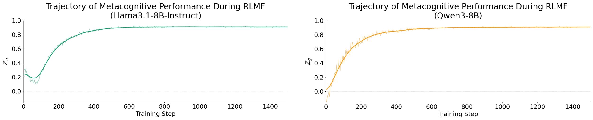
10.4 Example Generations↩︎
We provide illustrative examples of well-aligned and misaligned intrinsic and expressed uncertainty by LLMs. Examples for the numerical setting are shown in Fig.s 26 and 27. Good faithful alignment occurs when expressed and intrinsic confidence are either both high (e.g., \(>0.5\)) or both low (e.g., \(<0.5\)). Misalignment occurs when expressed confidence is high and intrinsic confidence is low, or vice versa.
We also provide representative examples of linguistic uncertainty with our approach versus the FUT baseline in Table ¿tbl:tab:examples?. It can be seen that while FUT leads to generic formulations, our approach
leads to more diverse and naturalistic outputs, confirmed via human evaluation (§11).
None
Figure 26: Example of well-aligned intrinsic and numerically expressed confidence, extracted from Llama3.1-8B-Instruct on the PopQA dataset following our Stage 1 training..
None
Figure 27: Example of poorly aligned intrinsic and numerically expressed confidence, extracted from Llama3.1-8B-Instruct without any special training procedures applied..
| Sample Generations (Ours) | Sample Generations () |
| The film was produced by Sophia Lin, though I’m not very confident in this answer. | It is quite likely that the producer of “Compliance" is unknown to me. |
| My best guess is that Compliance was produced by Magnolia Pictures, but I could easily be wrong. | It is somewhat doubtful that the producer of the 2012 film “Compliance" is Steven Soderbergh. |
| I vaguely recall that the producer might be tied to Oscilloscope Laboratories, but I wouldn’t stake much on that. | It is very likely that I do not have enough information to determine who produced “Compliance". |
| Sample Generations (Ours) | Sample Generations () |
| Pedalfer soils are associated with deciduous forests and rich in nutrients, have high fertility, and are typically yellow, brown, or reddish in color. | It is quite likely that the correct answer is alfisol or temperate forest soil. |
| I believe alfisols are the soils most commonly associated with temperate deciduous forests — they tend to be moderately fertile with a well-developed horizon structure — but I hold that with only moderate confidence. | It is somewhat doubtful that sandy soil is the correct answer. |
| My tentative understanding is that deciduous forests are often underlain by relatively nutrient-rich soils with significant organic matter in the upper horizons, though I can’t confidently name the specific soil order. | It is likely that the correct answer involves fertile, loamy soils with good organic content. |
11 Human Evaluation Study Details↩︎
We conducted a human annotation study to verify that responses produced via our approach are indeed more natural, helpful, context-adaptable, and preferred by humans versus the prior state-of-the-art SFT-based approach FUT[48]. Our annotation setup was as follows. We used three expert annotators (graduate students working directly with LLMs) and instructed them to provide preference
annotations on 120 examples. These examples were obtained by randomly drawing 20 samples each from Natural Questions [131], SciQ, and SelfAware and collecting responses from Llama3.1-8B-Instruct and Qwen3-8B, yielding \(3\times 20 \times 2 = 120\) combinations. Each dataset was paired with a specific
context and user preference specification (Fig. 28): Natural Questions with a conversational educational assistant context (A), SciQ with a research and fact-checking assistant context (B), and SelfAware—which includes
inherently unanswerable questions—with a high-stakes professional assistant context (C). For SciQ, which is originally multiple-choice, model responses were elicited without answer choices to encourage free-form uncertainty expression. During generation,
models were additionally provided with the corresponding user context specification rephrased in the first person as if written by the user, to prompt context-appropriate responses (as opposed to the third-person annotator-facing formulations shown in
Fig. 28).
During the annotation study, for each example, annotators were provided with the original query, its associated user context, 3 responses from the model trained via FUT, and 3 responses from the model trained with RLMF and
metacognitive data selection and rewritten via Stage 2, with the order and naming of each response set randomized. Annotators were asked to indicate which set of responses more helpfully, naturally, coherently, and context-appropriately communicated the
model’s uncertainty. In particular, annotators were tasked with providing 4 ratings per example, comparing the two sets of responses along 4 criteria. Ratings were collected via a custom annotation interface, and full task instructions and the list of
criteria are shown in Fig. 29. Prior to the main task, annotators completed 10 held-out examples to confirm understanding of the instructions and resolve potential misinterpretations. Annotators were informed
of the purpose, aims, and intended use of the study. We obtained informed consent from each annotator prior to their participation. No compensation was provided given the small-scale nature of the task.
We observed a high inter-annotator agreement of 0.93 as measured via Krippendorff’s alpha. Counting absolute wins with half-weight for ties, responses generated with our approach achieved win rates of 98%, 98%, 95%, and 96% in dimensions of diversity,
naturalness, helpfulness, and context suitability over those generated with FUT, providing compelling evidence for value of our approach toward holistic and practical faithful calibration of LLMs’ expressions of uncertainty.
None
Figure 28: Exact specifications of user preference and context provided to annotators per task setting..
None
Figure 29: Instructions given to annotators for the preference annotation task..
References↩︎
Our code is provided at https://github.com/yale-nlp/RLMF.↩︎
Versus claim- [52], [53] or response-level scoring [54], [55], sentence-level scoring [56] better balances computational efficiency, interpretability, and alignment with natural language structure [33].↩︎
Exact reward formulas, weighting, and implementation details can be seen in §9.1.1. Each reward’s criticality is also demonstrated via ablation study in §9.1.1.8.↩︎
We use the quadratic formulation of \(Z_g\) as it is empirically strongest; alternative formulations are possible and analyzed in §9.2.2.↩︎
The impact of alternatively applying \(Z_g\) as an additional reward function is explored in §9.2.2.4.↩︎
The impact of \(A^{\texttt{RLMF}}_g\) design, \(k\) value, \(\tau\) value are respectively analyzed in §9.2.2.3, §9.2.3, §9.2.4.↩︎
Details are in §8.1.0.3. We assess the contribution of the pre-SFT stage via ablation study in §9.1.6.↩︎
Example generations and results for sub-8B models are in §10.4; §10.1.↩︎
Note that improvement at self assessment of performance is not equivalent to broad metacognitive awareness, as metacognition encapsulates many other types of such capabilities.↩︎
RLMFimplementation details are available in our code at https://anonymous.4open.science/r/RLMF_anon.↩︎Early experiments showed a cosine schedule was superior to linear or constant schedules.↩︎
Recall from §3.1 that we use the completions sampled during GRPO in a dual-purpose fashion, both to provide a signal for preference optimization and since this naturally extends the sampling-based paradigm for intrinsic confidence estimation used in prior work on faithful calibration.↩︎
We use
nltkas it offers a widely-used and reliable sentence tokenizer.↩︎We sample equally from the ‘boolq’, ‘copa’, ‘wic’, and ‘wsc’ subsets in our experiments.↩︎
While we base these judgments on linguistically expressed confidence, in light of the end goal of our framework, use of similar judgments of numerically expressed confidence may be similar in efficacy.↩︎
The original paper used Gemini-2.0-Flash, but this model has since been deprecated for certain users; we considered Gemini-2.5-Flash-Lite as an appropriate substitute given its comparable capabilities↩︎
Existing work [56], [122] shows going beyond \(K=20\) yields marginal returns on estimate quality. More generally, \(K=10\) is determined to be sufficient for similar paradigms [82], [86], [123].↩︎
Note that [6] use assertions as the basis for consistency evaluation, whereas [48] use sentences and show that both levels are comparable. Given that our training task requires models to output sentence-level confidence scores, we follow [48] to adopt sentence-level scoring. This also bypasses the additional computation required for assertion extraction, originally used by [5] to disentangle factual content from hedging language, which is unnecessary here since no hedging language appears for our training task.↩︎
We use Qwen3-32B as it is this is a simple task for which prior work [6] deemed Gemini-2.0-Flash to be sufficiently capable; manual verification by the authors on a sample of 300 examples confirmed that Qwen3-32B achieves near 100% accuracy in performing such judgments while avoiding the cost incurred by querying a proprietary LLM at scale.↩︎
The originating paper used Gemini-2.0-Flash, but this model has been deprecated for certain users; we therefore adopt Gemini-2.5-Flash-Lite as an alternative which is comparable and still cost-efficient.↩︎
Early experiments considered alternative mathematical formulations, such as use of the linear absolute difference, the square root of the absolute difference, or cross entropy, but these were empirically less fruitful (see §9.1.2). We therefore adopt the quadratic formulation shown in Eq. 10 in this work.↩︎
Due to the preliminary nature of the investigation, we did not use metacognitive data selection or advantage scaling for these experiments, nor did we apply pre-SFT. GRPO was implemented without removing advantage normalization.↩︎
These experiments used the same procedure as described in §8.1.0.2, but with a smaller hyperparameter search, wherein we considered only learning rates of 5e-6 and 1e-5.↩︎
Recall that we obtain \(M\)’s self-predicted target task performance \(F_{\text{pred}}\) by querying \(M\) to issue a single float between 0 and 1 indicating its confidence that its numerically reported per-sentence confidences \(c_{1:N_g}\) are faithful to its per-sentence intrinsic confidences \(g_{1:N_g}\). An alternate approach is to obtain one such metacognitive judgment score per sentence and take the average as \(F_{\text{pred}}\). We did not do so due to the computational expense incurred by such a setup and since our current paradigm already achieves good results, but this presents another viable avenue for future exploration.↩︎
Recall from §3.2 that \(\tau\) is the threshold for comparing predicted and gold confidences when estimating \(F_{\text{gold}}\), the gold faithful calibration level of \(M\) for completion \(r_g\) used to compare with \(M\)’s self-predicted FC level \(F_{\text{pred}}\).↩︎
We accordingly use only inference-based \(F_{\text{pred}}\) scores in our main
RLMFsetup.↩︎Recall that this score is a value from 0–100. We use this range as opposed to 0.0–1.0 as early experiments showed models tended to cluster their issued metacognitive scores in a small range when the latter was used, similar to findings by prior work [109].↩︎
This is because our official strategy performs the best.↩︎
This is because active learning aims to improve performance by exposing the model to samples which present greater difficulty.↩︎
Empirically, use of bin size 0.1 and 0.05 did not yield meaningful differences in early experiments.↩︎