Surrogate Fidelity: When Can Open LLMs Explain Closed Ones?
June 30, 2026
Abstract
Mechanistic interpretability (MI) requires full access to model internals, yet the APIs for most widely deployed language models at best expose log-probabilities over output tokens. This creates a surrogate problem: when do measurements made on open models allow us to make claims about a closed model? We evaluate surrogate fidelity at the prediction, attribution, and representation levels. For binary classification tasks, log-odds provide an API-compatible scalar readout of the model’s representation space, and leave-one-out attributions provide insight into model behavior. Across eleven models spanning four families (Llama, Qwen, GPT, and Gemini), we find that prediction fidelity substantially overstates attribution fidelity: models that agree on what the answer is often disagree on why. We document an access–validity inversion: white-box signals like attention patterns and perturbation magnitudes are highly stable across models but only weakly predictive of causal attributions, which black-box input ablations capture by design. Mechanistic insight does not automatically transfer to closed targets, and prediction-level agreement is insufficient to warrant such transfer. Code and results are available at https://github.com/facebookresearch/surrogate.
1 Introduction↩︎
The models that most urgently need mechanistic interpretability (MI) are precisely those least amenable to it. Most classical MI tools, such as circuit analysis, sparse autoencoders, and activation patching, require full access to model internals. Meanwhile, most users of frontier large language models (LLMs) access text completions from behind APIs that, at best, offer log-probabilities for a handful of high-likelihood tokens. This creates a bifurcation: MI research is either conducted by frontier labs within the walled gardens of their own models, or by academic groups studying small open models and hoping their findings generalize. The broader community of practitioners, safety researchers, and auditors is left to wonder what can be learned about a model we cannot open from studying one we can.
This assumption that mechanistic insights transfer across models is implicit, pervasive, and under-examined in the literature. If it is wrong, then open-source MI work may be telling us less than we think about the frontier models we most need to understand. We argue that the field needs an open dialogue about cross-model fidelity, grounded in a shared convention for measurement that is realistic about the distinction between closed and open models.
We define a surrogate fidelity metric as a measure of how faithfully a measurement in a surrogate model predicts a measurement in a target model. A surrogate fidelity metric should be appropriately scoped (dataset- and claim-dependent), discriminative between different model pairs, and governed by the principle of least privilege, i.e. it should require no more access to the target model than the claim being evaluated demands. In particular, at least some surrogate fidelity measurements should be computable using top-\(K\) log-probabilities alone: a constraint consistent with the APIs of many frontier model providers.
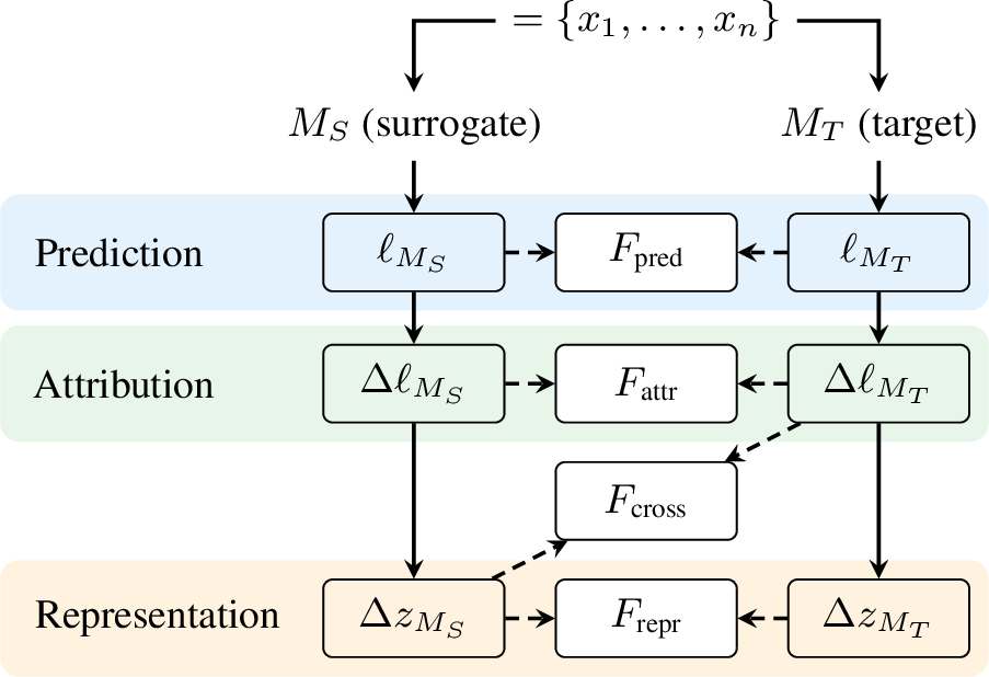
To this end, we propose a hierarchy of increasingly strict tests as a concrete starting point for measuring surrogate fidelity, drawing on established MI intuitions and practices. Prediction fidelity for outputs; attribution fidelity for output-level responses to causal interventions (input ablations); representation fidelity for representation-level responses to the same interventions; and cross-level fidelity for predicting the target’s attributions from the surrogate’s internal representations. This progression from observational to interventional to mechanistic agreement echoes the causal hierarchy of [1], grounding each level in a concrete, measurable test of surrogate faithfulness.
Our contributions. Our contributions are as follows:
We argue that the MI community’s implicit assumption that mechanistic findings transfer across models deserves direct scrutiny, and propose surrogate fidelity as a conceptual framework for this dialogue.
We propose a hierarchy of surrogate fidelity metrics—prediction, attribution, representation, and cross-level—instantiated for binary classification benchmarks. Prediction and attribution require only top-\(K\) log-probabilities, while representation- and cross-level fidelity require open-weight model access.
Evaluating two open-weight families (Qwen 2.5, Llama 3) and two closed-API families (GPT, Gemini) across multiple scales (0.5B–70B parameters) on three binary classification benchmarks, we find a striking dissociation: models that share similar representations and predictions can nonetheless disagree sharply on causal attributions.
We identify an access–validity inversion: high-agreement white-box signals like attention and perturbation magnitude fail to predict more causally relevant black-box attributions.
2 Preliminaries↩︎
Throughout this section, all quantities are implicitly conditioned on a single input and its representation \(z\) in model \(M\); we make these dependencies explicit in 3 when comparing across models and inputs.
2.1 Static geometry↩︎
We review the geometric relationship between a transformer’s residual stream and its output probabilities, establishing the quantities on which our fidelity metrics operate.
Given a representation \(z \in \mathbb{R}^d\) in a transformer’s residual stream, the logit for token \(t\) is the dot product \[\mathrm{logit}_t = z \cdot u_t,\] where \(u_t \in \mathbb{R}^d\) is the column of the unembedding matrix \(W_U \in \mathbb{R}^{d \times V}\) corresponding to token \(t\). The output probability is computed via softmax: \[P(t) = \frac{\exp(z \cdot u_t)}{\sum_{i=1}^{V} \exp(z \cdot u_i)}.\] Thus, the log-probability of any token is \(\log P(t) = z \cdot u_t - C\), where \(C = \log \sum_{s=1}^{V} \exp(z \cdot u_s)\) is the log of the softmax normalization constant. Without access to the full vocabulary of logits, \(C\) is not recoverable from a handful of top-\(K\) log-probabilities.
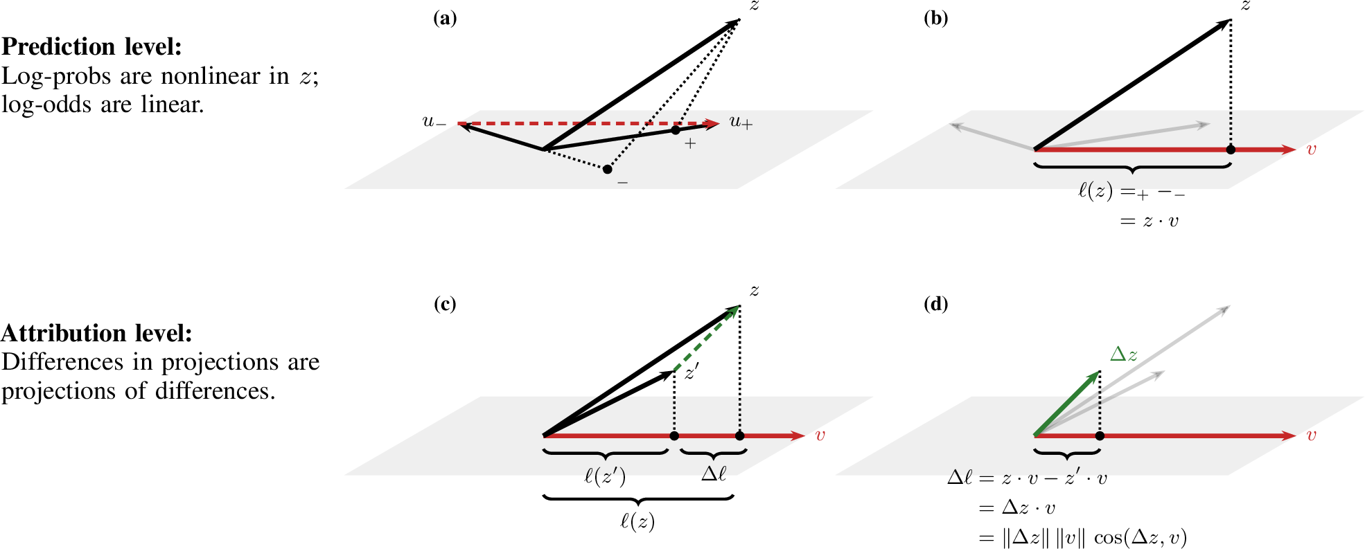
Since \(C\) is shared across all logits, when we take the difference of two log-probabilities, \(C\) cancels out: \[\begin{align} \log P(t) - \log P(s) &= (z \cdot u_t - C) - (z \cdot u_s - C) \nonumber \\ &= z \cdot (u_t - u_s). \label{eq:log95odds95linear} \end{align}\tag{1}\] Defining the readout (log-odds) direction \(v = u_+ - u_-\) for a binary classification task with positive and negative class tokens, the log-odds reduce to a single dot product: \[\ell(x) = z \cdot v. \label{eq:log95odds}\tag{2}\] While individual log-probabilities are nonlinear functions of \(z\), the log-odds are exactly linear in the representation. This is the key observation that makes our fidelity framework possible: log-odds are both API-accessible (as a difference of two log-probabilities) and geometrically interpretable (as a projection onto a readout direction in representation space). 2 (a–b) illustrates this progression from individual logits to the log-odds direction.
2.1.0.1 Residual stream decomposition.
The residual stream of a transformer is a running sum: after layer \(l\), the state is \(z^{(l)} = z^{(0)} + \sum_{k=1}^{l}(a^{(k)} + m^{(k)})\), where \(z^{(0)}\) is the token embedding and \(a^{(k)}, m^{(k)} \in \mathbb{R}^d\) are the outputs of the attention and MLP sublayers at layer \(k\). Because log-odds are linear in \(z\), this additivity extends directly to the prediction: projecting any intermediate state \(z^{(l)} \cdot v\) yields a valid log-odds estimate at depth \(l\) — the logit lens [2] — while decomposing the final projection term by term yields direct logit attribution (DLA) [3]. Writing out both relationships: \[\begin{align} z^{(L)} &= z^{(0)} + \sum_{l=1}^{L} \left(a^{(l)} + m^{(l)}\right) \tag{3} \\ \ell(x) &= z^{(0)} \cdot v + \sum_{l=1}^{L} \left(a^{(l)} \cdot v + m^{(l)} \cdot v\right). \tag{4} \end{align}\] The first line is the residual stream; the second is the same equation projected onto \(v\). The logit lens reads the partial sums \(z^{(l)} \cdot v\) cumulatively across depth; DLA reads the individual terms \(a^{(l)} \cdot v\) and \(m^{(l)} \cdot v\) as per-component contributions to the final log-odds. We investigate the DLA of predictions and attributions in 11.
2.2 Intervention and attribution↩︎
For an intervention1 that changes the representation from \(z\) to \(z'\), the resulting change in log-odds is: \[\Delta\ell = \ell(z) - \ell(z') = \Delta z \cdot v, \label{eq:attribution}\tag{5}\] where \(\Delta z = z - z'\) is the perturbation in the residual stream. We call \(\Delta\ell\) the attribution of the intervention. Concretely, attribution measures the causal effect of changing the input on \(\ell\); it is not a complete internal mechanism.
Because attribution is a dot product, it decomposes into three factors: \[\Delta\ell = \|\Delta z\|\; \|v\|\; \cos(\Delta z, v). \label{eq:factorize95attribution}\tag{6}\] Since \(\|v\|\) is fixed for a given model and task, attribution is governed by two properties of the perturbation: its magnitude \(\|\Delta z\|\) and its alignment \(\cos(\Delta z, v)\) with the log-odds direction. A large perturbation orthogonal to \(v\) produces zero attribution; a small perturbation aligned with \(v\) can shift the prediction substantially. 2 (c–d) illustrates this geometry.
Eqs. 5 –6 are exact when \(z\) and \(z'\) are the post-normalization representations that the unembedding matrix sees.
The role of LayerNorm. In closed models, \(\Delta \ell\) only reveals information about the post-normalization representations \(z\) and \(z'\). In practice, however, interventions perturb the pre-normalization residual stream \(\hat{z}\). For a normalization \(z \to \hat{z}\,/\,f(\hat{z})\) that acts by scalar rescaling2, the post-normalization perturbation decomposes further as: \[\Delta z = \underbrace{\frac{\Delta\hat{z}}{f(\hat{z})}}_{\text{direct}} \;+\; \underbrace{\hat{z}'\,\frac{f(\hat{z}') - f(\hat{z})}{f(\hat{z})\,f(\hat{z}')}}_{\text{indirect}}. \label{eq:norm95decomp}\tag{7}\] The direct term is the pre-normalization perturbation \(\Delta\hat{z}\) rescaled by the baseline normalization factor, i.e. the contribution that would remain if \(\hat{z}'\) was normalized by the original norm \(\|\hat{z}\|\). The indirect term arises because changing \(\hat{z} \to \hat{z}'\) also changes the normalization denominator, effectively rescaling the entire post-normalization representation \(z'\). This term is nonzero whenever \(f(\hat{z}) \neq f(\hat{z}')\) and \(\hat{z}' \cdot v \neq 0\), even if \(\Delta\hat{z}\) itself is orthogonal to \(v\).
3 Method↩︎
We formalize surrogate fidelity at three levels of increasing depth: do two models make similar predictions, produce similar attributions under the same perturbations, and share internal representations? Each level imposes a stricter test of whether mechanistic insights transfer across model families.
Prediction and attribution fidelity require only log-probabilities and are therefore computable for any model pair, including closed targets; representation fidelity additionally requires access to model internals.
Let \(M_S\) and \(M_T\) denote surrogate and target models, and \(\mathcal{D} = \{x_1, \ldots, x_n\}\) an evaluation corpus. For each model \(M\), the quantities defined in 2 — log-odds \(\ell_M(x)\), attributions \(\Delta\ell_M(x, i)\), perturbation norms \(\|\Delta z_M(x, i)\|\), and alignments \(\gamma_M(x, i) = \cos(\Delta z_M, v_M)\) — are stacked over all prompts and segments to form vectors (denoted in boldface). We additionally write \(\alpha_M(x, i)\) for attention-based importance scores. Throughout, agreement is measured by \(r^2\) with bootstrapped 95% confidence intervals.
Prediction fidelity measures agreement on outputs: \[F_\text{pred}(M_S, M_T; \mathcal{D}) = r^2\!\left( \boldsymbol{\ell}_{M_S},\; \boldsymbol{\ell}_{M_T} \right). \label{eq:f95pred}\tag{8}\]
Attribution fidelity measures agreement on causal importance under leave-one-out ablation: \[F_\text{attr}(M_S, M_T; \mathcal{D}) = r^2\!\left( \boldsymbol{\Delta\ell}_{M_S},\; \boldsymbol{\Delta\ell}_{M_T} \right). \label{eq:f95attr}\tag{9}\] High \(F_\text{pred}\) with low \(F_\text{attr}\) signals that models agree on outputs while disagreeing on which inputs drive them, a critical failure mode for surrogate-based interpretability.
For open-weight models, we can additionally define representation-level metrics, referred to generically as \(F_\textrm{repr}\). The decomposition in 6 motivates two representation fidelity metrics measuring agreement in perturbation magnitude and alignment respectively: \[\begin{align} F_\text{mag}(M_S, M_T; \mathcal{D}) &= r^2\!\left( \|\boldsymbol{\Delta z}_{M_S}\|,\; \|\boldsymbol{\Delta z}_{M_T}\| \right), \tag{10} \\ F_\text{align}(M_S, M_T; \mathcal{D}) &= r^2\!\left( \boldsymbol{\gamma}_{M_S},\; \boldsymbol{\gamma}_{M_T} \right). \tag{11} \end{align}\] Attention patterns have also been used as a proxy for mechanistic importance [4]; we include attention fidelity as a third representation-level metric: \[F_\text{attn}(M_S, M_T; \mathcal{D}) = r^2\!\left( \boldsymbol{\alpha}_{M_S},\; \boldsymbol{\alpha}_{M_T} \right). \label{eq:f95attn}\tag{12}\] For attention, we consider several attention aggregation strategies (mean, max, rollout; see 4).
Finally, cross-level fidelity asks whether the surrogate’s internals predict the target’s attributions: \[F_\text{cross}(M_S, M_T; \mathcal{D}) = r^2\!\left( \boldsymbol{\alpha}_{M_S},\; \boldsymbol{\Delta\ell}_{M_T} \right). \label{eq:f95cross}\tag{13}\] For closed \(M_T\), \(F_\text{cross}\) quantifies whether mechanistic analysis of an open \(M_S\) yields actionable insight about \(M_T\).
Readout-compatible linear transfer. Our use of Pearson \(r^2\) is motivated by a readout-compatible notion of representation transfer. Concretely, for idealized models \(M_S, M_T\) related through a readout-compatible linear transformation, i.e. \(z_T \approx A z_S\) and \(A^T v_T \approx cv_S\), \[\label{eq:linear95transform} z_T \cdot v_T \approx A z_S \cdot v_T = z_S \cdot (A^T v_T) \approx c(z_S \cdot v_S) = c\ell_S,\tag{14}\] i.e. the log-odds of \(M_S\) and \(M_T\) are in a perfect linear relation. The same holds for \(\Delta \ell\), yielding \(\Delta \ell_T \approx c \Delta \ell_S\).
Thus, \(r^2\) measures the fraction of variation explained by \(M_S\) under the simplest readout-compatible linear calibration. Low \(r^2\) in a single dimension rules out high-fidelity transfer under such a readout-compatible \(A\), though it leaves open weaker forms of representational similarity.
Analogous correlation-based measures exist in higher dimensions: the RV coefficient [5] for multivariate readouts and centered kernel alignment (CKA) [6] for full representations. This lineage grounds our use of \(r^2\) as a readout-level probe into overall representational similarity and motivates our multi-class extension in 16.
| Metric | Open\(\to\)Open \(\r\) | Open\(\to\)Closed \(\r\) | All\(\to\)All \(\r\) | |
|---|---|---|---|---|
| Black-box | \(F_{\mathrm{pred}}\) | \(.177\,/\,\mathbf{.652}\,/\,.795\) | \(.108\,/\,\mathbf{.682}\,/\,.845\) | \(.108\,/\,\mathbf{.709}\,/\,.956\) |
| \(F_{\mathrm{attr}}\) | \(.091\,/\,\mathbf{.432}\,/\,.560\) | \(.032\,/\,\mathbf{.420}\,/\,.557\) | \(.032\,/\,\mathbf{.460}\,/\,.828\) | |
| Representation-level | \(F_{\mathrm{attn}}^{\mathrm{mean}}\) | \(.762\,/\,\mathbf{.905}\,/\,.984\) | — | — |
| \(F_{\mathrm{mag}}\) | \(.641\,/\,\mathbf{.855}\,/\,.903\) | — | — | |
| \(F_{\mathrm{attn}}^{\mathrm{rollout}}\) | \(.443\,/\,\mathbf{.848}\,/\,.938\) | — | — | |
| \(F_{\mathrm{attn}}^{\mathrm{max}}\) | \(.641\,/\,\mathbf{.842}\,/\,.910\) | — | — | |
| \(F_{\mathrm{align}}\) | \(.058\,/\,\mathbf{.200}\,/\,.294\) | — | — | |
| Cross-level | \(F_{\mathrm{align} \to \mathrm{attr}}\) | \(.060\,/\,\mathbf{.259}\,/\,.381\) | \(.032\,/\,\mathbf{.262}\,/\,.362\) | \(.032\,/\,\mathbf{.259}\,/\,.381\) |
| \(F_{\mathrm{mag} \to \mathrm{attr}}\) | \(.000\,/\,\mathbf{.074}\,/\,.229\) | \(.000\,/\,\mathbf{.122}\,/\,.282\) | \(.000\,/\,\mathbf{.109}\,/\,.282\) | |
| \(F^{\mathrm{mean}}_{\mathrm{attn} \to \mathrm{attr}}\) | \(.000\,/\,\mathbf{.004}\,/\,.035\) | \(.000\,/\,\mathbf{.003}\,/\,.024\) | \(.000\,/\,\mathbf{.003}\,/\,.035\) | |
| \(F^{\mathrm{rollout}}_{\mathrm{attn} \to \mathrm{attr}}\) | \(.000\,/\,\mathbf{.003}\,/\,.069\) | \(.000\,/\,\mathbf{.002}\,/\,.013\) | \(.000\,/\,\mathbf{.002}\,/\,.069\) | |
| \(F^{\mathrm{max}}_{\mathrm{attn} \to \mathrm{attr}}\) | \(.000\,/\,\mathbf{.002}\,/\,.032\) | \(.000\,/\,\mathbf{.002}\,/\,.019\) | \(.000\,/\,\mathbf{.002}\,/\,.032\) |
4 Evaluation Setting↩︎
This is a summary of our experimental setup; full details can be found in the Appendix, 9.
4.1 Benchmarks↩︎
We focus our initial investigation on binary classification tasks: when a model’s output space is \(\{y^+, y^-\}\), the log-odds \(\ell_M(x)\) collapse to a single scalar per prompt, providing a compact and interpretable summary of the model’s internal decision boundary.
Binary classification is practical under API constraints: the top-\(K\) most likely tokens are typically constrained to a small, predictable set of label variants. In more open-ended settings, we expect significantly more missing values.
We evaluate on three binary classification benchmarks spanning distinct reasoning capabilities:
BoolQ [7]: Boolean question answering over Wikipedia passages (validation split; \(n{=}3{,}270\)). Tests reading comprehension with yes/no questions.
ANLI [8]: Adversarial natural language inference (test splits R1/R2: \(n{=}1{,}000\) each, R3: \(n{=}1{,}200\)). Progressively harder rounds constructed to fool strong models, providing a difficulty gradient.
WinoGrande [9]: Debiased coreference resolution (validation split; \(n{=}1{,}267\)). Binary choice between candidate referents. Also serves as our primary testbed for ablation experiments.
Beyond our core binary classification experiments, we also extend our evaluation framework to two other benchmarks:
LAMBADA [10]: Word prediction requiring broad discourse context (test split; \(n{=}5{,}153\)). We score completion log-probability rather than log-odds, providing a robustness check across scoring methods.
RACE [11]: Multiple-choice reading comprehension (test split; \(n{=}4{,}934\), 4 choices per question). We report RV coefficients on pairwise log-odds.
4.2 Models↩︎
We compare models across four families and multiple scales:
Llama [12]: Llama 3.1-8B, Llama 3.1-70B, Llama 3.3-70B, Llama 4 Maverick
Qwen [13]: Qwen-0.5B, Qwen-3B, Qwen-7B, Qwen-14B
GPT [14]: GPT-4o, GPT-4.1
Gemini [15]: Gemini 2.5 Flash Lite
The Llama and Qwen families provide multiscale open-weight models, enabling representation-level extraction (for \(F_\text{repr}\) and \(F_\text{cross}\)) and investigation into how surrogate fidelity scales with model size. GPT and Gemini models are accessible only through black-box APIs exposing top-\(K\) log-probabilities, restricting us to \(F_\text{pred}\) and \(F_\text{attr}\) for these targets. Notably, the Claude and GPT-5 families, which do not expose any log-probabilities to end users, are excluded from this evaluation.
4.3 Ablation protocol↩︎
For attribution fidelity, we segment each prompt and remove individual segments to produce ablated inputs \(\tilde{x}_i\). We evaluate at two granularities:
Sentence-level: Each sentence in the prompt constitutes a segment. Coarser but less expensive, as each prompt yields few ablations.
Word-level: Each whitespace-delimited token is a segment. Finer-grained but requires substantially more model queries per prompt.
Sentence-level ablations are applied to all benchmarks; word-level ablations are applied to a downsampled subset (\(n{=}10{,}000\)) of each benchmark due to cost constraints.
5 Results↩︎
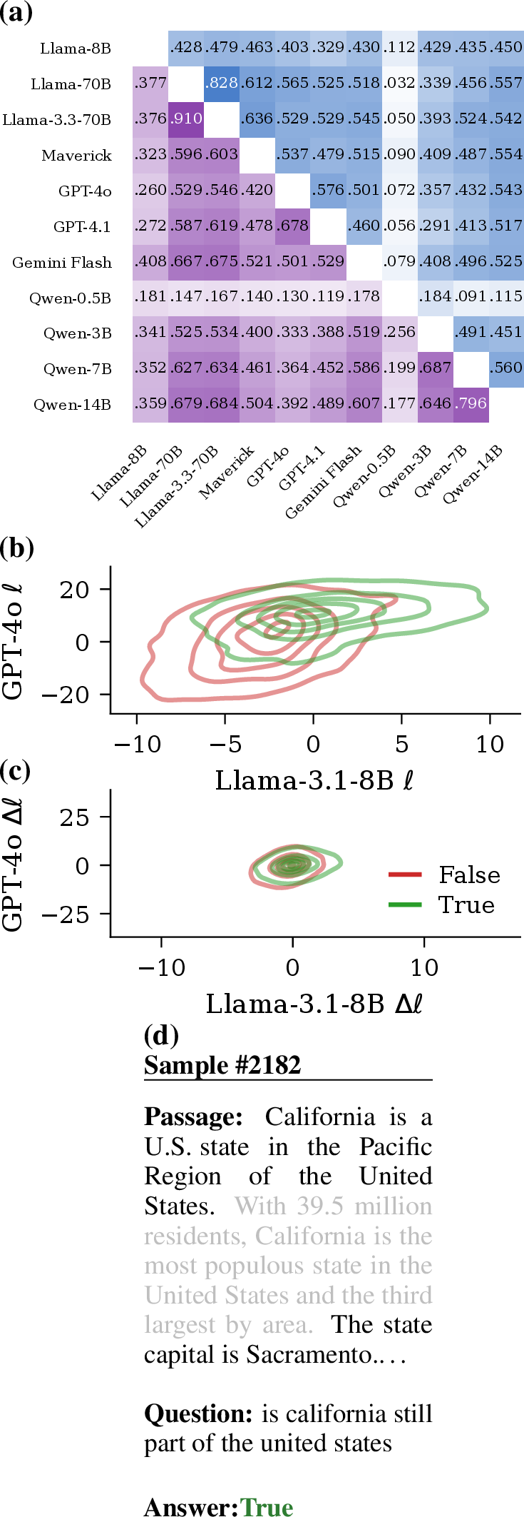
We first evaluate prediction and sentence-level attribution fidelity on the BoolQ validation set across all eleven models. We report pairwise \(r^2\) values in 1 and show the full pairwise fidelities and cross-family contour plots for \(F_\mathrm{pred}\) and \(F_\mathrm{attr}\) in 3, as well as an example BoolQ prompt.
5.1 Prediction fidelity↩︎
Prediction fidelity is high within families but drops substantially across families. Predictably, Llama 3.1-70B and Llama 3.3-70B have high mutual \(F_\mathrm{pred}\) (\(0.910\)) and exhibit similar \(F_\mathrm{pred}\) profiles generally. The same is true for Qwen-7B and Qwen-14B (\(0.796\)) and GPT-4o and GPT-4.1 \((0.678)\). By contrast, the highest cross-family \(F_\mathrm{pred}\) is between Llama 3.1-70B and Qwen 2.5-14B at \(0.684\); cross-family ranges are generally slightly lower.
Notably, Qwen-0.5B is an outlier on all fronts, with low prediction fidelity to any models including larger models in the Qwen family. This is consistent with its uniquely small size among the evaluated models, and is contextualized by the generally low confidence and poor log-probability separation reported in 8 in the Appendix.
5.2 Attribution fidelity↩︎
For each model and each BoolQ prompt, we computed sentence-level ablations and measured the attribution fidelity across model pairs.
At this level, attribution agreement is strikingly low across all model pairs, even within-family. The median within-family \(F_\mathrm{attr}\) is only \(0.432\), and even the closest pair (Qwen-7B vs Qwen-14B) only achieves a \(F_\mathrm{attr}\) score of \(0.560\).
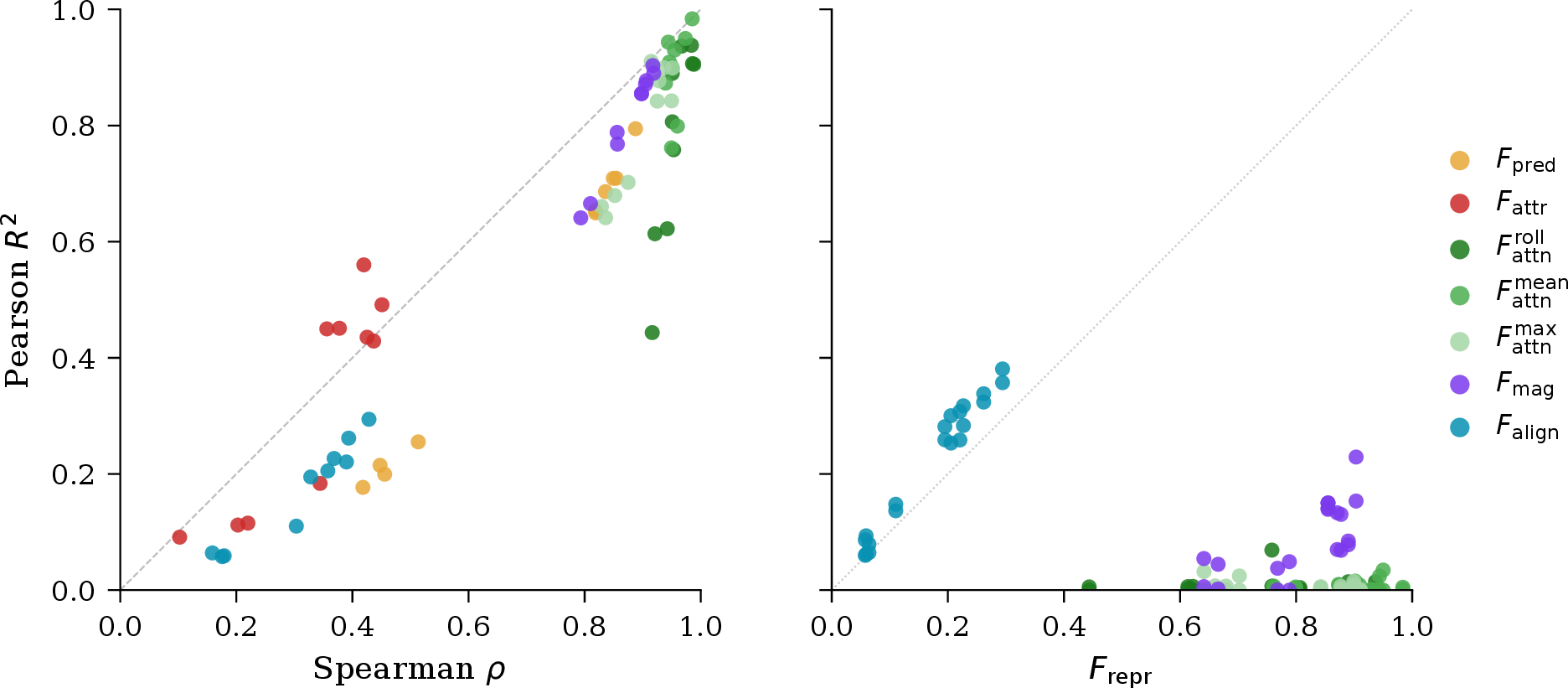
Unlike \(F_\mathrm{pred}\), where \(r^2\) closely tracks Spearman \(\rho\), \(r^2\) values for \(F_\mathrm{attr}\) are slightly higher than Spearman \(\rho\) (see 9 in Appendix), as they are significantly more stable in the presence of near-zero attributions.
Word-level validation. To rule out that the low ablation agreement is an artifact of sentence-level coarseness, we repeat the analysis at word level, using leave-one-out single deletion [16] of individual whitespace tokens. We subsample 10,000 (prompt, word) ablation pairs per model from a pool of 476,154 possible BoolQ word ablations using a shared random seed.
Per Table 2, switching from sentence- to word-level ablation leaves mean and rollout attention fidelity mostly unchanged but sharply reduces \(F_{\mathrm{attr}}\) (from \(.460\) to \(.175\)), driven almost entirely by the collapse of \(F_{\mathrm{align}}\) (\(.200 \to .012\)). The attribution signal fractures at finer resolution; the representational signals do not.
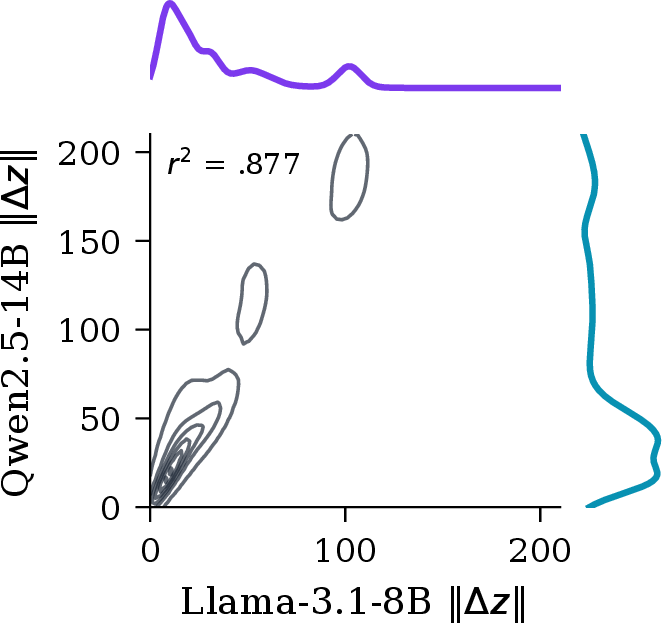
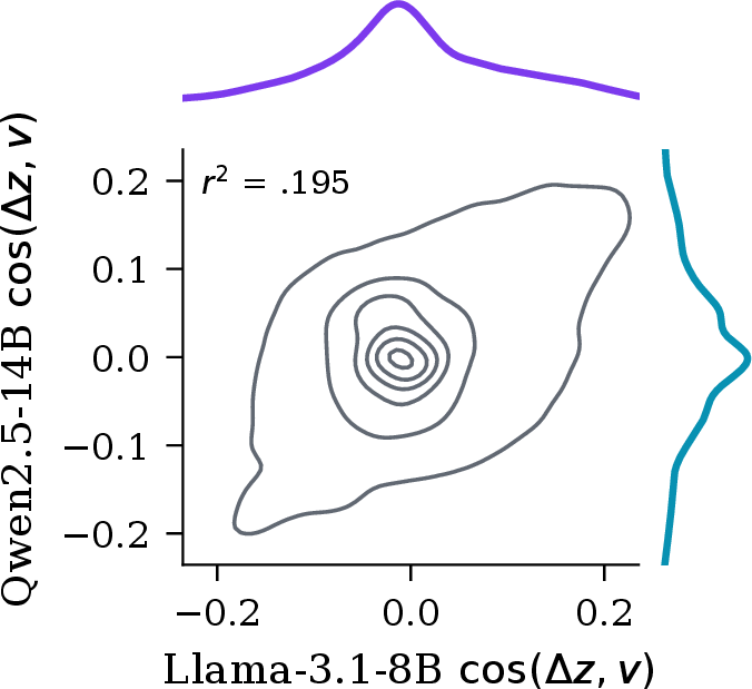
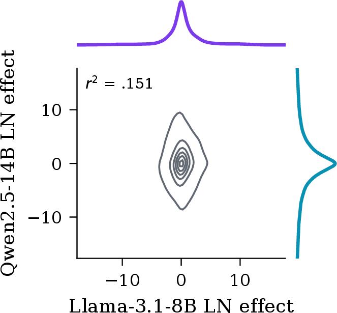
Figure 4: Perturbations affect attribution through their norm (left), alignment with the log-odds direction \(v\) (middle), and indirectly via LayerNorm (right). We plot joint and marginal distributions of each, for a representative model pair..
5.3 Representational fidelity↩︎
In this section, we focus both on decomposing \(F_\mathrm{attr}\) according to the components of attribution (norm of perturbation, angle between perturbation and readout direction, and LayerNorm-induced rescaling) and investigating the role attention could play in surrogate model predictions.
Decomposing attributions. 4 shows that models’ responses to perturbations are stable in magnitude (high \(F_\mathrm{mag}\)) but not direction (low \(F_\mathrm{align}\)). This suggests that low \(F_\mathrm{attr}\) is driven primarily by disagreement in the direction of the perturbation-response vector \(\Delta z\). The maximum cosine similarity between \(\Delta z\) and \(v\) tops out around 0.4, with most cosine similarities landing near zero. Using unsigned cosine similarity does not improve \(F_\mathrm{align}\).
While most perturbations have negligible effects on log-odds from the perspective of the projection of \(\Delta z\) onto \(z\), it is also possible for perturbations to affect a model’s log-odds through the LayerNorm’s rescaling of the overall vector, as rescaling a vector by \(\alpha\) also rescales \(\ell\) by \(\alpha\).
We find that roughly 15–23% of each attribution is due to LayerNorm rescaling, with the rest explainable by the unnormalized change in representation. Interestingly, the direction of LayerNorm rescaling is essentially uncorrelated with attribution, meaning that while this component of the model architecture can contribute to lower \(F_\mathrm{attr}\) scores, it is unlikely to bias it in a specific direction. For models \(\geq\)3B parameters, there is no clear trend in terms of the LayerNorm’s contribution to \(\Delta \ell\), with Llama 3-8B sitting in the middle of the Qwen results across all metrics.
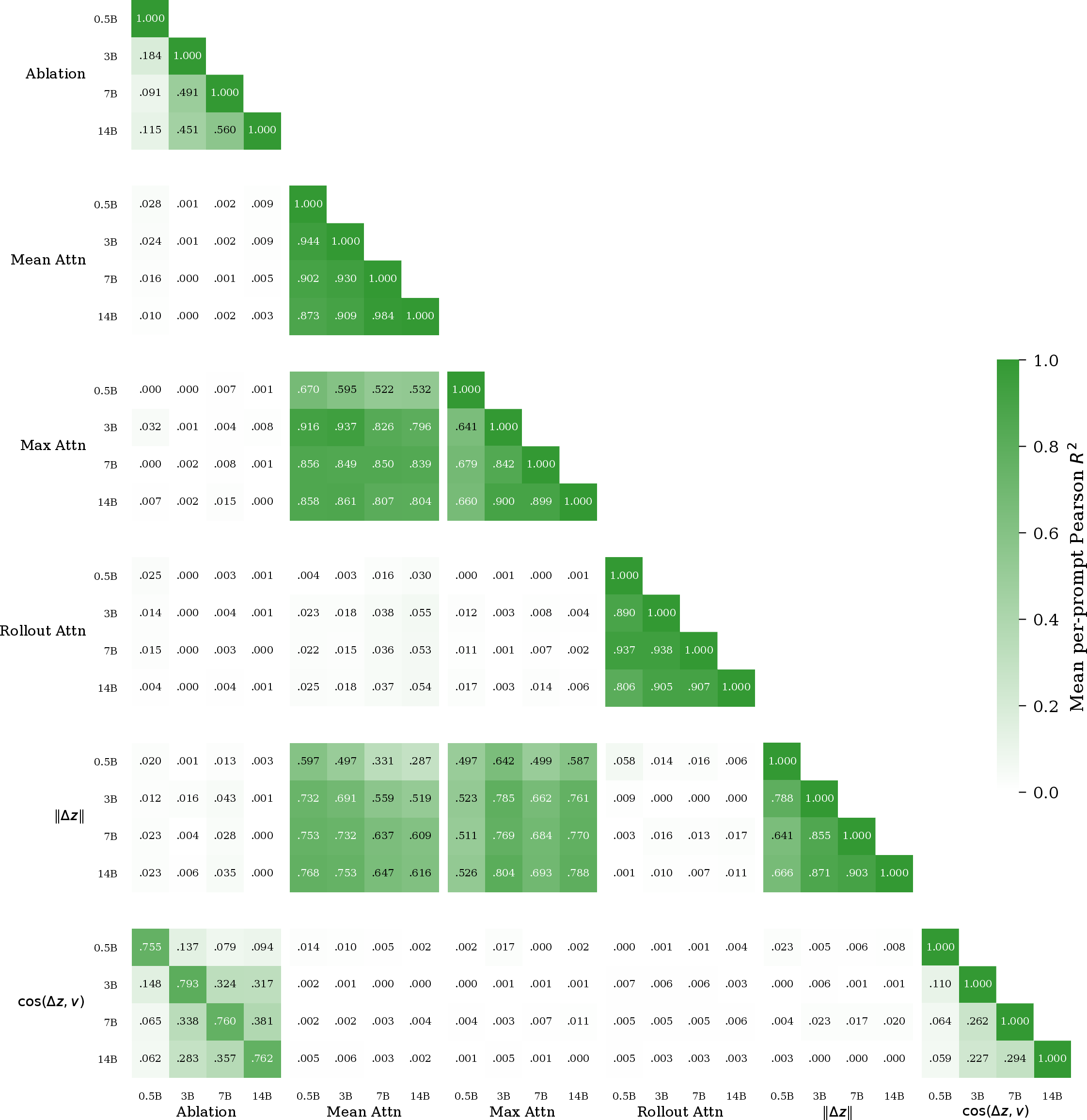
Attention: stable but limited. In contrast to ablation attributions, attention-based scores exhibit strong agreement across the board. Mean attention correlations range from \(r^2= 0.762\) to \(0.984\), and attention rollout, which accounts for residual connections across layers [4], achieves median \(r^2= 0.848\). Even Qwen-0.5B, which was an outlier for prediction and attribution fidelity, attends to the same tokens as its larger siblings.
Despite high within-method consistency, the three attention aggregation strategies are not interchangeable. Mean and max attention correlate moderately (\(r^2\approx 0.473\)–\(0.969\)), but rollout attention is almost uncorrelated with these (\(r^2\approx 0.045\)–\(0.215\)). This methodological sensitivity underscores the importance of specifying the aggregation scheme when reporting attention-based results.
The contrast between high representational fidelity and low attribution fidelity reveals a dissociation: models can share attention patterns while diverging in causal structure. Attention consistency (often used as informal evidence that “models are doing the same thing”) is a weak proxy for the mechanistic agreement that MI practitioners actually need.
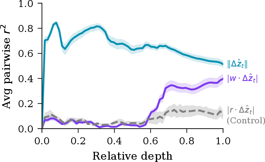
Per-layer fidelity. We track the per-layer variants of \(F_\mathrm{mag}^{(l)}\) and \(F_\mathrm{attr}^{(l)}\) of the metrics defined in 10 9 in 5. A clean depth dissociation emerges: high representation-level agreement across most depths, but low attribution-level agreement for the first \({\sim}55\%\) of depth with a subsequent sharp rise. This pattern could be a generic property of late-layer perturbations, so we include a random direction control—replacing \(v\) with a per-model random unit direction \(r\) matched in norm to \(\|v\|\). The random-direction control rises late as well—the \(v\)-specific premium over the random baseline at the readout layer is therefore \({\approx}0.29\) in \(r^2\). We read this as a partial qualification of our claim that low \(F_\mathrm{attr}\) reflects models “disagreeing on which inputs drive their predictions.” See 11 for extended experiments, analysis, and experiment setup.
| Metric | BoolQ | ANLI R1 | ANLI R2 | ANLI R3 | WinoGrande | BoolQ word | LAMBADA | RACE |
|---|---|---|---|---|---|---|---|---|
| \(F_{\mathrm{pred}}\) | \(.709\) | \(.354\) | \(.282\) | \(.343\) | \(.225\) | \(.708\) | \(.108\) | \(.462\) |
| \(F_{\mathrm{attr}}\) | \(.460\) | \(.280\) | \(.223\) | \(.241\) | \(.150\) | \(.175\) | \(.115\) | \(.524\) |
| \(F_{\mathrm{attn}}^{\mathrm{rollout}}\) | \(.848\) | \(.852\) | \(.853\) | \(.854\) | \(.850\) | \(.857\) | \(.690\) | \(.811\) |
| \(F_{\mathrm{attn}}^{\mathrm{mean}}\) | \(.905\) | \(.953\) | \(.951\) | \(.954\) | \(.871\) | \(.881\) | \(.561\) | \(.913\) |
| \(F_{\mathrm{attn}}^{\mathrm{max}}\) | \(.842\) | \(.939\) | \(.937\) | \(.937\) | \(.808\) | \(.627\) | \(.332\) | \(.842\) |
| \(F_{\mathrm{mag}}\) | \(.855\) | \(.867\) | \(.875\) | \(.874\) | \(.671\) | \(.524\) | \(.342\) | \(.771\) |
| \(F_{\mathrm{align}}\) | \(.200\) | \(.078\) | \(.071\) | \(.060\) | \(.018\) | \(.012\) | \(.024\) | \(.100\) |
| \(F_{\mathrm{align} \to \mathrm{attr}}\) | \(.259\) | \(.128\) | \(.113\) | \(.114\) | \(.051\) | \(.026\) | \(.040\) | \(.183\) |
| \(F_{\mathrm{mag} \to \mathrm{attr}}\) | \(.109\) | \(.297\) | \(.268\) | \(.305\) | \(.228\) | \(.173\) | \(.159\) | \(.319\) |
| \(F^{\mathrm{rollout}}_{\mathrm{attn} \to \mathrm{attr}}\) | \(.002\) | \(.021\) | \(.016\) | \(.011\) | \(.017\) | \(.004\) | \(.007\) | \(.014\) |
| \(F^{\mathrm{mean}}_{\mathrm{attn} \to \mathrm{attr}}\) | \(.003\) | \(.013\) | \(.013\) | \(.022\) | \(.018\) | \(.003\) | \(.099\) | \(.036\) |
| \(F^{\mathrm{max}}_{\mathrm{attn} \to \mathrm{attr}}\) | \(.002\) | \(.013\) | \(.016\) | \(.010\) | \(.022\) | \(.002\) | \(.069\) | \(.033\) |
5.4 Additional experiments↩︎
We report our results for the ANLI, WinoGrande, LAMBADA, and RACE benchmarks in 2.
Across binary classification benchmarks, the qualitative ordering is stable: \(F_\mathrm{pred}\) generally exceeds \(F_\mathrm{attr}\), attention is stable, and \(F_\mathrm{mag}\) is more stable than \(F_\mathrm{align}\). Surprisingly, we do not find a monotonic relationship between ANLI difficulty (R1 \(<\) R2 \(<\) R3) and most fidelity statistics, suggesting that fidelity measurements may be insensitive to task difficulty. WinoGrande fidelity is lower across \(F_\mathrm{pred}\) and \(F_\mathrm{attr}\), and shows higher \(F_\mathrm{cross}\) for mean- and max-pooled attention. LAMBADA results show unusually low \(F_\mathrm{pred}\) and \(F_\mathrm{attr}\), suggesting that the change in last-token log-probabilities may behave differently from log-odds.
While \(r^2\) and RV scores are not directly comparable, the RACE results mostly resemble binary classification. Interestingly, \(F_\mathrm{attr}\) is modestly larger than \(F_\mathrm{pred}\) (0.524 vs 0.462), consistent with 25, which shows that perturbation RV scores exceed representation RV scores in high dimensions. These results may be confounded by longer prompts and the larger spread of pairwise log-odds.
In the Appendix, 10 contains expanded visualizations and calibration results, 11 contains full per-layer logit lens results, 12 demonstrates confidence-dependence in fidelity measurements, 13 proposes normalized root mean squared error (NRMSE) as an asymmetric variant of \(r^2\), 14 elaborates on the mechanistic causes of the prediction–attribution gap, 15 studies the effect of additionally modifying models’ system prompts, 16 extends our analysis to multiple-choice benchmarks, and 17 makes the connection to CKA explicit.
6 Discussion↩︎
The access-validity inversion. While \(F_\mathrm{pred}\) measures prediction-level agreement, attribution fidelity is causal: leave-one-out ablations amount to a coarse-grained gradient of the prediction with respect to context, so mechanistic agreement requires this stricter condition beyond basic prediction agreement. For all model pairs not including Qwen 2.5–0.5B, \(F_\mathrm{pred}> F_\mathrm{attr}\), and \(F_\mathrm{attr}\) is generally very low.
Furthermore, we find most representation-level properties to have limited ability to predict attributions. API-compatible attribution metrics are more causally relevant than some white-box signals. In fact, median \(F_\mathrm{repr}\) and \(F_\mathrm{cross}\) are very poorly aligned (see 9), implying representation-level transfer is largely uncorrelated with causal prediction. These negative results on attention add to the growing literature reexamining its explanatory value [17]–[19].
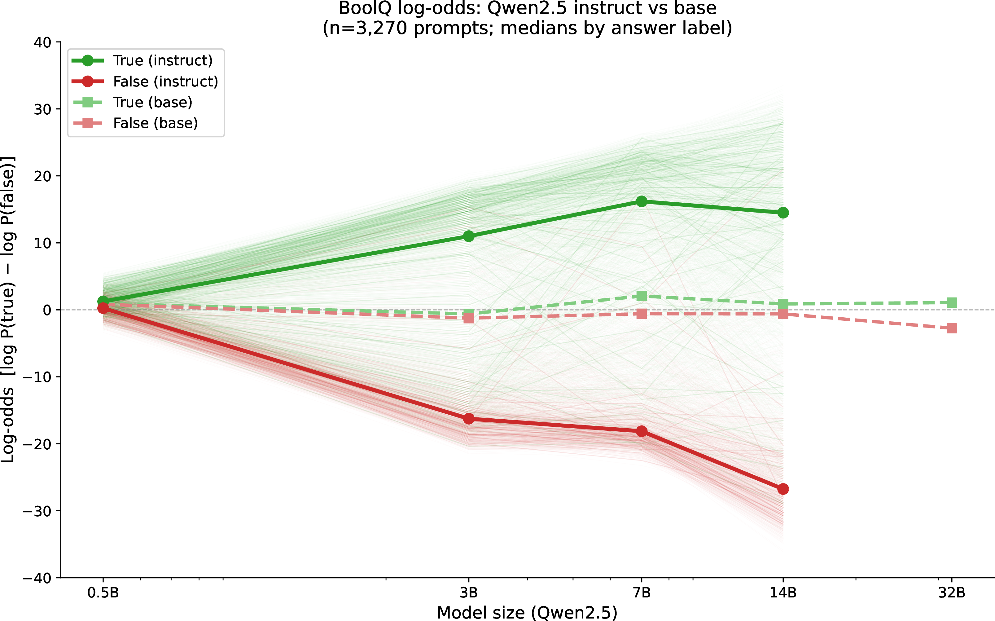
A plausible explanation for the access-validity inversion is that training forces models to align representations in high-probability subspaces, but the null space of the top-\(K\) readouts is less constrained. Consequently, models may agree on their overall predictions and even gross structural response (\(F_\mathrm{mag}\)) while pointing in very different directions. Interestingly, this divergence is detectable with only API-level access: you can’t see how these representations differ, but you can see that they do. (Since we observe that log-probs diverge between true and false prompts only in instruction fine-tuned models (see 10.2), it’s even possible that the access-validity inversion is posttraining-specific.)
Surrogate fidelity as local linear geometry. The Platonic Representation Hypothesis [20] holds that models converge to a shared representation, citing evidence such as model stitching, which unifies two models’ representations via a learned linear transformation (similar to the \(A\) discussed in 14 ). Under this framing, our results are ironic: while appearances do indeed converge (high \(F_\mathrm{pred}\)), the Forms themselves actually fan out across different models (low \(F_\mathrm{align}\)).
The polytope lens relaxation [21] affords models freedom to shuffle operations within closed consistency regions, so low surrogate fidelity need not imply deep representational divergence. This more closely matches how [20] actually demonstrate their claims, eschewing the strict orthogonal transformation assumptions underpinning CKA in favor of nearest-neighbor overlaps.
Practical guidance. Our results imply that surrogate validity must be measured rather than assumed, and suggest a concrete way for practitioners to make surrogate validity claims. Prediction fidelity is a useful screen, but it consistently overstates agreement at the level needed for explanation: on BoolQ with word-level ablations, \(F_\mathrm{pred}= 0.708\) whereas \(F_\mathrm{attr}= 0.175\). Representational similarities can also be misleading. For instance, \(F_\mathrm{mag}\) and \(F_\mathrm{attn}^\mathrm{}\) are high across model pairs, suggesting high similarity more generally, but directional alignment breaks the pattern: \(F_\mathrm{align}\) is consistently low, driving down \(F_\mathrm{attr}\) with it.
The appropriate fidelity test depends on the level of access and the claim being made. Both \(F_\mathrm{pred}\) and \(F_\mathrm{attr}\) can be measured using log-probabilities alone, and should be reported whenever comparing models to make claims about surrogate explanations. For directly testing open-to-closed mechanism transfer, \(F_\mathrm{cross}\) requires open-weight access to the surrogate. In our evaluation, no surrogate-side representation signal clears this bar. Validating at the level of the explanation being made and the behavior being tested will help ground claims about generalization to frontier models. Note that the intervention can and should be chosen to match the behavior of interest: for instance, leave-one-out ablations are useful for claims about input evidence or saliency, but may not be appropriate for circuit-level claims.
Limitations and future work. Our framework is a first step towards standardized surrogate fidelity evaluation; we expect practices to evolve with input from the MI community.
We focus on binary classification tasks where log-odds give a reliable readout, with exploratory extensions into last-token and multiple-choice settings. An extension to open-ended text generation, which represents the vast majority of LLM use cases and does not admit an obvious scalar summary, is a natural next step requiring new scoring functions.
Our focus on leave-one-out attribution trades mechanistic depth for API compatibility; moreover, ablations shifting inputs off-distribution may have unintended side effects. It is therefore natural to extend our work to more commonly used representation-level interventions like activation patching, richer mechanistic signals (steering vectors, SAE features), and meaning-preserving input perturbations [22]. Low cross-seed consistency between SAE features [23], [24] might imply similarly low representation fidelity.
7 Related Work↩︎
Feature attribution for LLMs. Leave-one-out attribution [25], ContextCite [26], and local surrogate methods such as MExGen [27] and gSmILE [28] estimate input-level importance for generative models. AttriBoT [29] scales attribution to long contexts via efficient approximation. These methods only explain what a model’s prediction depends on; we connect attributions to internal mechanism by exploiting the linearity of log-odds. In this regard, [30] is also influential to our work in its use of log-probabilities to probe model mechanisms.
Proxy and surrogate models. Prior work asks whether proxy models can cheaply approximate a target’s predictions [31] or attributions [32], [33], often by training or fine-tuning a surrogate. On the other hand, we ask when a surrogate-derived explanation is valid evidence about a target model’s mechanism.
Mechanistic interpretability. Circuit analysis [3], [34] has been scaled [35], [36] and automated [37]; sparse autoencoders offer a complementary feature-level decomposition [38]–[40]. Causally relevant directions—steering vectors [41]–[43], linear probes [44], [45], crosscoder latents [46]–[48]—identify features that influence behavior but require full model access. We relax this requirement and test whether surrogate-derived features transfer to closed targets.
Attention as explanation. Attention weights are widely used as explanations but their validity is contested [17]–[19], [49], [50]. Our \(F_{\mathrm{cross}}\) metric provides direct evidence: attention patterns are highly consistent across scales yet uncorrelated with causal attributions, so attention stability is not evidence of mechanistic agreement.
Representation similarity. CKA [6], SVCCA [51], and RSA [52] compare hidden representations across models. The linear representation hypothesis [53] and polytope lens [21] characterize how models encode concepts geometrically. Our results partially agree: attention converges across scales, but its dissociation from attribution fidelity shows representational convergence does not imply functional equivalence.
8 Conclusion↩︎
We introduce a hierarchy of surrogate fidelity metrics (prediction, attribution, and representational) grounded in the distinction between observational, causal, and structural agreement. We find that neither prediction– nor representation-level fidelity implies attribution fidelity. When interpreting open surrogates as proxies for closed systems, we recommend that practitioners validate surrogates at the level of analysis they intend to perform, and release our evaluation framework to support this practice. More broadly, we offer an opinionated first proposal and invite the MI community to refine it: cross-model fidelity deserves to be discussed explicitly, and the right framework to measure it may still need to evolve.
9 Experimental Details↩︎
9.0.0.1 Models.
We evaluate the Qwen2.5 model family [13] at four scales: 0.5B, 3B, 7B, and 14B parameters, using the instruction-tuned variants
(Qwen2.5-{0.5B,3B,7B,14B}-Instruct). For the scaling analysis in Section 10.2, we additionally evaluate the base (non-instruction-tuned) variants at the same scales plus 32B. All models are loaded in bfloat16
precision on a single NVIDIA A100 80 GB GPU using HuggingFace Transformers [54] with device_map="auto". Models are
loaded and unloaded sequentially to fit within GPU memory.
9.0.0.2 Inference.
We extract logits from a single forward pass with no sampling—we do not generate text. For each prompt, we compute the log-softmax over the full vocabulary at the last token position (i.e., the position where the model would begin generating). This differs from API-based approaches that return only the top-\(k\) log-probabilities; our local inference provides exact log-probabilities for any token. Temperature is not applicable as we operate on raw logits without sampling.
9.0.0.3 Log-odds scoring.
For a prompt \(x\) and label classes \(\mathcal{P}\) (positive) and \(\mathcal{N}\) (negative), we define the log-odds as: \[\ell(x) = \log \sum_{t \in \mathcal{P}} P(t \mid x) - \log \sum_{t \in \mathcal{N}} P(t \mid x)\] where \(P(t \mid x)\) is the next-token probability for token \(t\). For BoolQ, \(\mathcal{P}\) and \(\mathcal{N}\) correspond to the tokens “true” and “false” respectively. To handle tokenizer variation, we expand each label
to include case variants (true, True, TRUE) and prefix variants (no prefix, space prefix, underscore prefix), yielding 9 token variants per label. Log-probabilities across variants are aggregated via log-sum-exp.
For ANLI, \(\mathcal{P}\) and \(\mathcal{N}\) correspond to token prefixes “ent” and “contr” (with the same case/prefix expansion); for WinoGrande, “1” and “2” (no expansion needed for single digits).
9.0.0.4 Prompt templates.
Each benchmark uses a task-specific system prompt and a structured user prompt. For BoolQ:
System: “You are a general-purpose binary question-answering machine. You will be shown a passage (marked ‘Context’), followed by a true/false question (marked ‘Question’) about that passage. Answer the question on the basis of the context, and respond only with ‘true’ or ‘false’.”
User: “Context: {passage}. Question: {question}.”
ANLI uses “Premise” / “Hypothesis” labels with an entailment/neutral/contradiction instruction; WinoGrande uses “Sentence” / “Option 1” / “Option 2” with a blank-filling instruction. Prompts are formatted using each model’s native chat template via
tokenizer.apply_chat_template().
9.0.0.5 Segmentation.
We segment prompts using Captum’s InterpretableInput framework [55]. For sentence-level experiments, we use the
"sentence" TextSegmentInput; for word-level experiments, the "word" TextSegmentInput. Segmentation operates on the user message text only (not the system prompt).
9.0.0.6 Ablation scoring.
For each prompt, we perform leave-one-out ablation: for each of \(N\) segments, we remove that segment and re-score the modified prompt. The ablation response for segment \(i\) is: \[a_i(x) = \ell(x) - \ell(x_{\setminus i})\] where \(x_{\setminus i}\) is the prompt with segment \(i\) removed. This requires \(N + 1\) forward passes per prompt (one for the original, one per ablation).
9.0.0.7 Attention scoring.
We extract attention weights from a single forward pass with output_attentions=True. Each transformer layer \(l\) produces an attention matrix \(A^{(l)} \in \mathbb{R}^{H \times T
\times T}\) where \(H\) is the number of heads and \(T\) is the sequence length. We consider three aggregation strategies:
Mean pooling: Average over all heads and layers, then extract the last row (attention from the prediction position to all input tokens).
Max pooling: Maximum over all heads and layers, then extract the last row.
Attention rollout [4]: At each layer, average over heads, mix 50/50 with the identity matrix (accounting for residual connections), renormalize rows, and multiply into a running product. The result captures attention flow through the full network.
Token-level attention is aggregated to segment-level scores by summing attention weights over the tokens belonging to each segment (mapped via tokenizer offset positions).
9.0.0.8 Agreement metrics.
Cross-model agreement is measured via Pearson correlation: for each benchmark, we concatenate all scalar measurements into a single vector and compute \(r^2\). All reported correlations include bootstrapped 95% confidence intervals (\(B = 1{,}000\) resamples of the per-prompt correlation distribution).
9.0.0.9 Benchmarks.
We evaluate on five benchmarks: BoolQ [7] (3,270 validation examples), ANLI [8] R1/R2/R3 (1,000/1,000/1,200 test examples), and WinoGrande [9] (1,267 validation examples).
9.0.0.10 Compute.
All experiments are run on a single NVIDIA A100 80 GB GPU. Sentence-level scoring (attention + ablation) for one benchmark \(\times\) four models takes approximately 2–4 hours depending on dataset size. Word-level ablation is substantially more expensive (\({\sim}100\times\) more forward passes) and runs for approximately 24 hours per benchmark.
10 Additional results↩︎
10.1 Detailed cross-representation agreement heatmap↩︎
A detailed heatmap of attention scoring methods and their agreement with \(F_\mathrm{attr}\) as cross-predictors is given in 6.
10.2 Output log-odds scaling in Qwen↩︎
We plot the log-odds of 100 randomly-selected prompts over different Qwen model sizes, as well as the true- and false-class medians, in 7. We repeat this process for base and instruct models, and find that instruct fine-tuning appears to drive log-odds differentiation in models.
10.3 Base log-odds distribution↩︎
In 8, we plot histograms of base log-odds distributions for different models on the BoolQ dataset. Histogram bars are subdivided by the proportion of true and false responses (ground truth) in the corresponding bin. Note that Qwen-0.5B has a highly irregular distribution compared to the rest of the models; this is a likely explanation for why it has extremely low \(F_\mathrm{pred}\) with all other models.

10.4 Metric calibration↩︎
In 9, we compare Spearman \(\rho\) and \(r^2\), as well as \(F_\mathrm{repr}\) and \(F_\mathrm{cross}\) scores, in open models. Each point represents one pair of distinct open models.
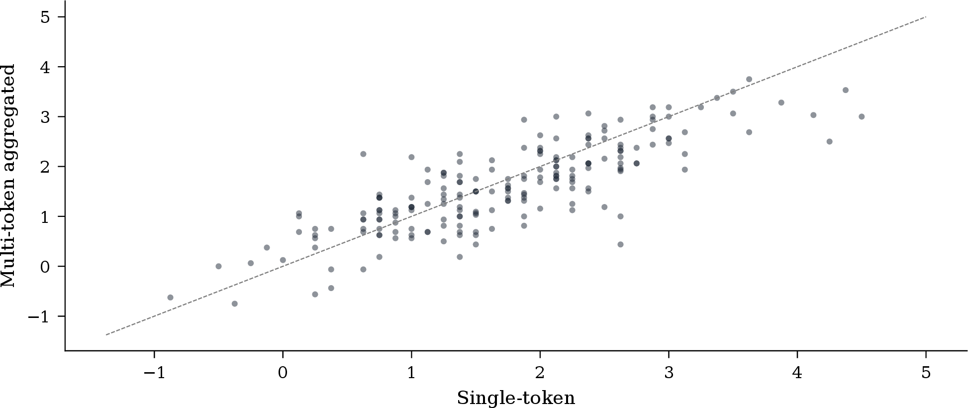
10 shows that the log-sum-exp over variants of the “True” token in BoolQ is highly correlated with the individual “true” vs “false” direction. In practice, only a single difference of unembeddings is linear; the log-add-exp breaks this nonlinearity. Because these quantities are so similar to one another, we do not expect significant issues from this approximation.
11 Per-layer fidelity trajectories↩︎
We extend the surrogate-fidelity framework of 3 from the final layer to every layer of the residual stream, asking at which depth the cross-model agreement on each fidelity level emerges. Throughout, we use the logit lens [2] convention introduced in 2: for every \(l \in \{0, 1, \ldots, L\}\) we read \(\ell^{(l)}(x) := \mathcal{N}(z^{(l)}) \cdot v\) where \(\mathcal{N}\) is the model’s final RMSNorm applied to the layer-\(l\) residual; index \(0\) is the embedding-layer projection \(\mathcal{N}(z^{(0)}) \cdot v\) and indices \(1, \ldots, L\) are the post-block residuals.3 Per-layer arrays therefore have length \(L + 1\). We use the open-weight subset of the model pool (Qwen-2.5 {0.5B, 3B, 7B, 14B}-Instruct and Llama-3.1-8B-Instruct), the BoolQ validation split (\(n = 500\) prompts), and the same sentence-level segmenter as 4, yielding \(2{,}105\) \((\mathrm{\small prompt}, \mathrm{\small segment})\) pairs that all five models share.
11.1 Trajectories of \(\ell^{(l)}\) and the lens distribution↩︎
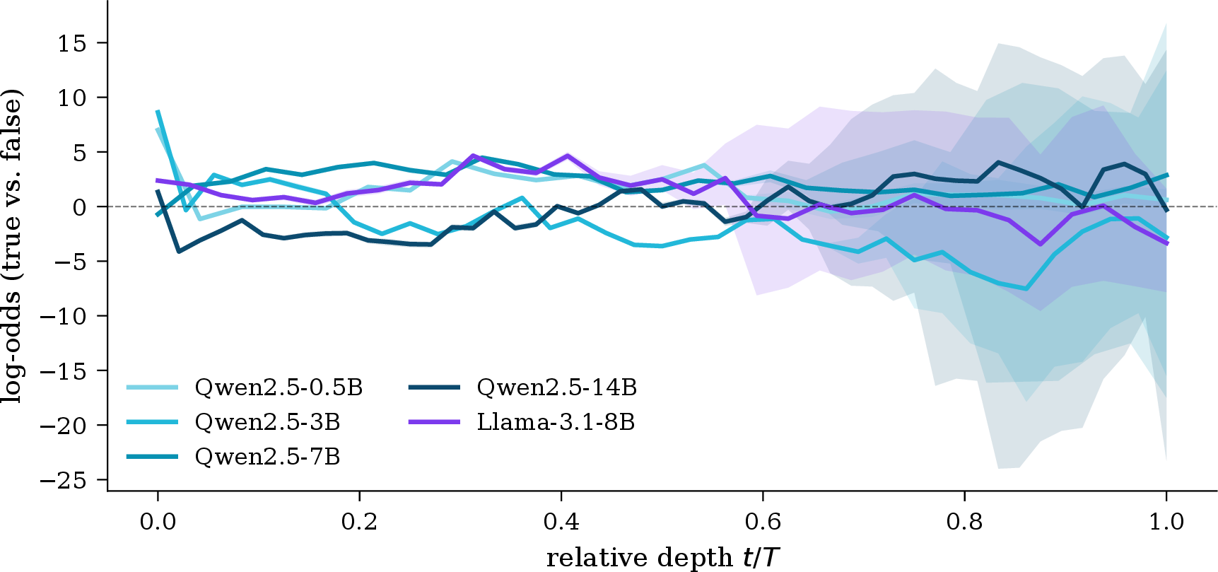
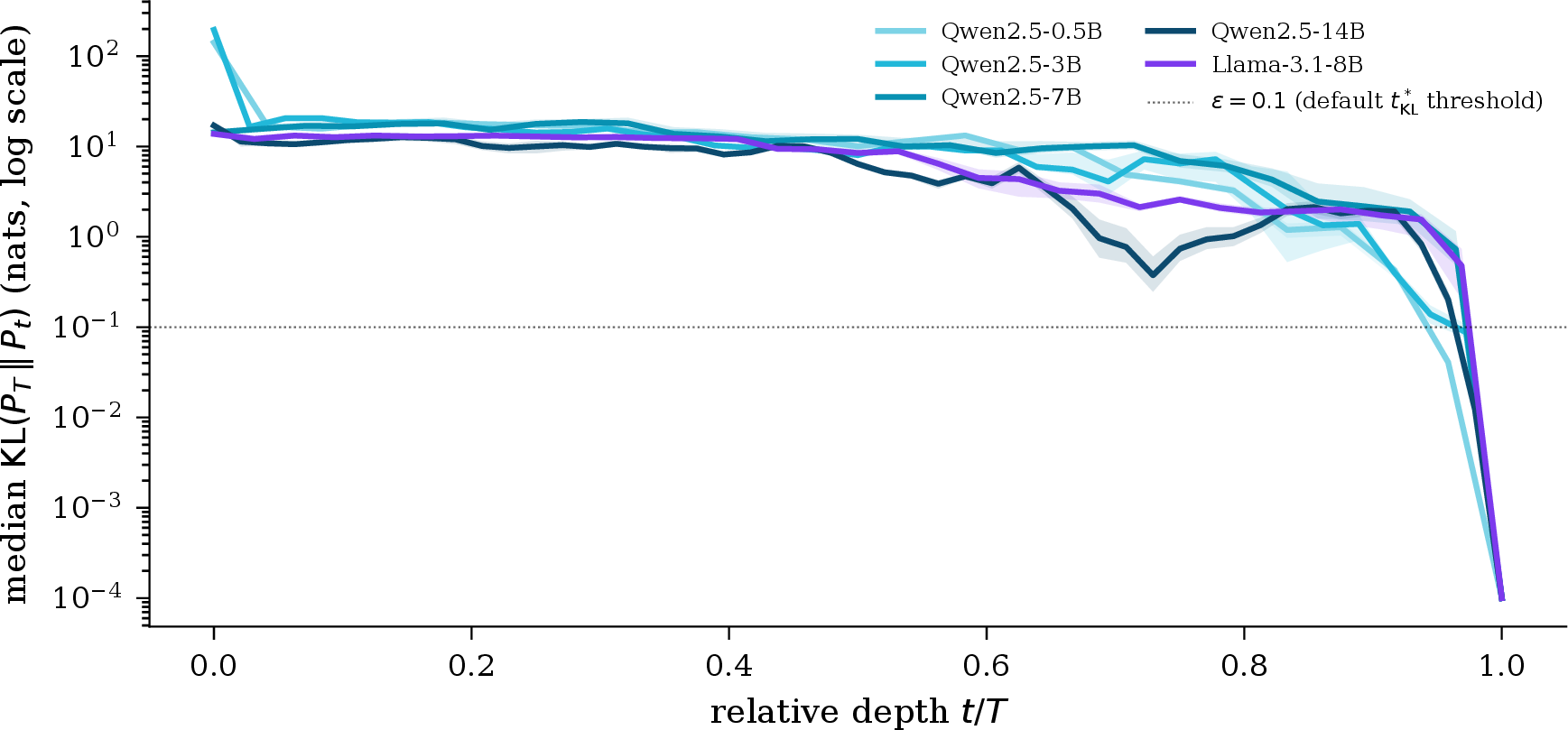
Figure 11: Per-layer trajectories and KL.. a — Median \(\ell^{(l)}\) (with IQR ribbons) per relative depth \(l / L\) across \(n = 500\) BoolQ prompts. Trajectories converge through relative depths \(0.1\)–\(0.5\) and re-diverge in the back half., b — Median \(\mathrm{KL}\big(P^{(L)} \,\|\, P^{(l)}\big)\) per relative depth, where \(P^{(l)} = \mathrm{softmax}(W_U^\top \mathcal{N}(z^{(l)}))\) is the lens distribution at layer \(l\). The final-layer distribution is reached only in the last 1–3 layers under any reasonable threshold (the dotted line marks \(\varepsilon = 0.1\) nats).
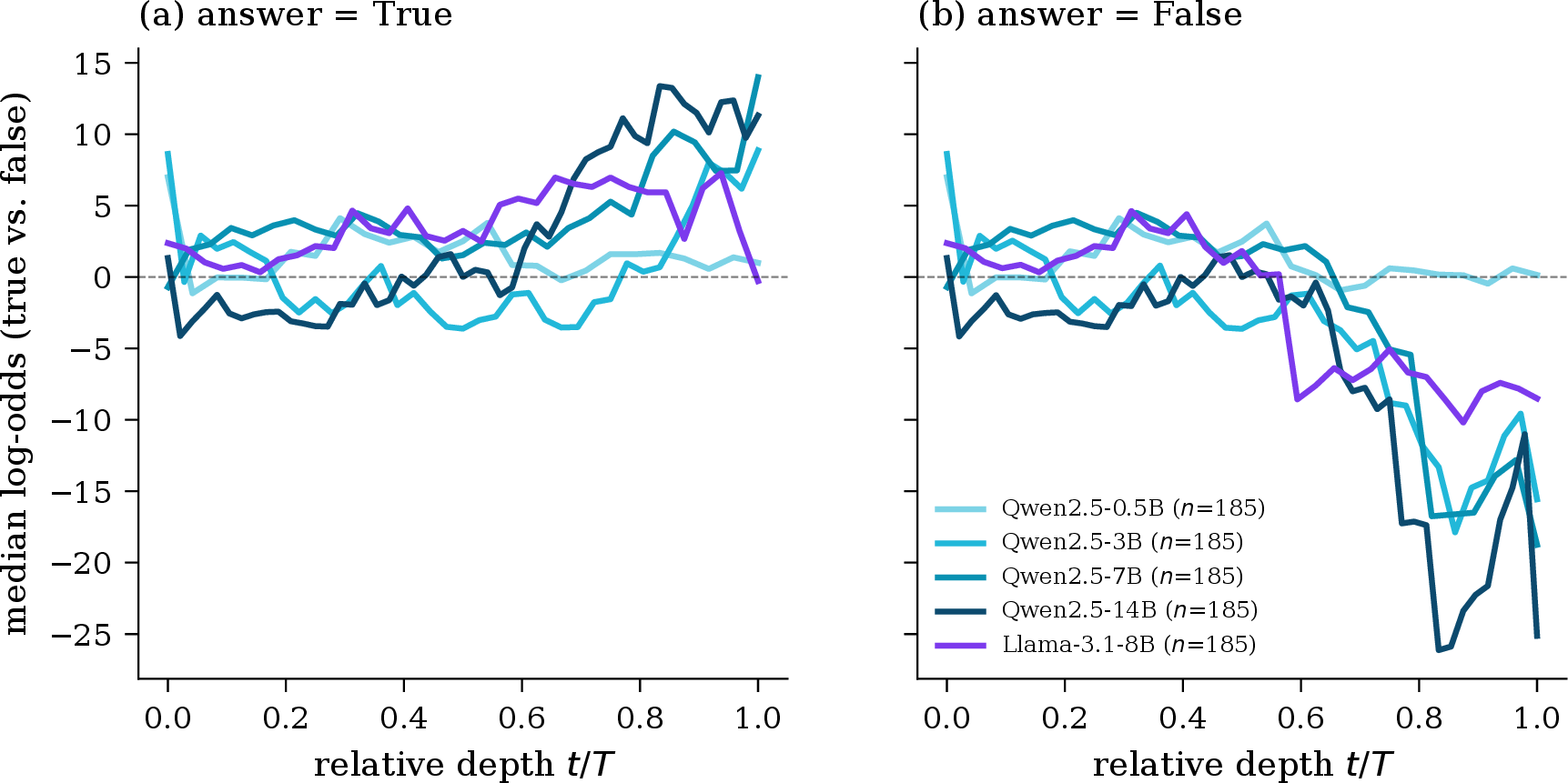
11 (a) plots the per-layer trajectories of \(\ell^{(l)}\). All five models start with a substantial embedding-layer bias whose sign and magnitude depend on the model’s static embedding of the assistant-marker token at the prediction position; readers should treat the layer-\(0\) slot as a per-tokenizer baseline rather than a content-dependent prediction. 12 splits the same trajectories by the ground-truth answer: the expected sign separation between the True- and False-prompt sub-populations emerges almost entirely in the back half of depth. 11 (b) summarizes the same data as the per-layer \(\mathrm{KL}\big(P^{(L)} \,\|\, P^{(l)}\big)\) — the lens distribution falls within \(0.1\) nats of the final-layer distribution only in the last 1–3 layers for every model.
11.2 Per-layer attribution decomposition↩︎
Following the factorization in 6 we record three per-\((\mathrm{\small prompt}, \mathrm{\small segment}, \mathrm{\small layer})\) scalars under the same leave-one-out segment ablation as 3: \(\|\Delta z^{(l)}\|\), \(\Delta\ell^{(l)} = \Delta z^{(l)} \cdot v\), and \(\cos(\Delta z^{(l)}, v)\), where \(\Delta z^{(l)} := \mathcal{N}(z^{(l)}(x)) - \mathcal{N}(z^{(l)}(\tilde{x}))\). [fig:per_layer:dnorm,fig:per_layer:wdotdz,fig:per_layer:cos] show the per-model medians.
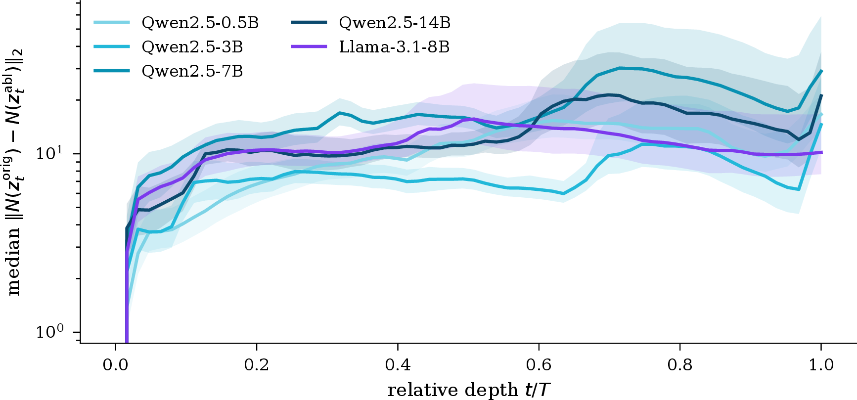
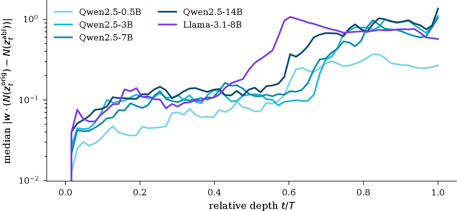
Figure 13: Per-layer structural perturbation norm and readout-aligned attribution magnitude.. a — Median \(\|\Delta z^{(l)}\|\) per relative depth. The structural footprint of an ablation appears almost immediately (depth \(\lesssim 0.1\)) and stays roughly flat thereafter., b — Median \(|\Delta\ell^{(l)}|\) per relative depth. The readout-aligned component is small (\({\sim}0.05\)–\(0.1\)) for the first half of depth and grows by 1–2 orders of magnitude in the last 30% of layers.
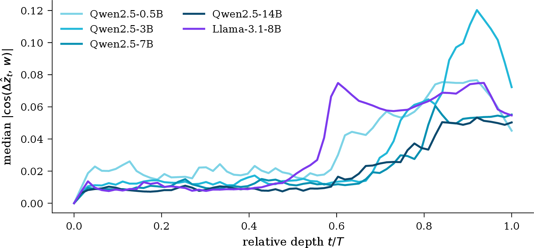
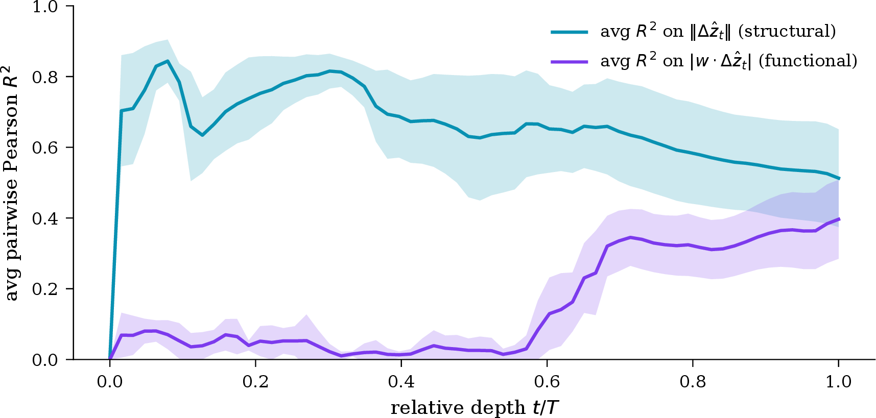
Figure 14: Per-layer directional alignment and pair-averaged attribution magnitudes.. a — Median \(|\cos(\Delta z^{(l)}, v)|\) per relative depth. Comparing with 13 (a) 13 (b) shows that the late rise in \(|\Delta\ell^{(l)}|\) is driven by the rising \(|\cos|\) factor of 6 , not by larger perturbations., b — Pair-averaged \(F_\mathrm{mag}^{(l)}\) (cyan, structural) and \(F_\mathrm{attr}^{(l)}\) (purple, functional) versus relative depth, with \(\pm 1\sigma\) ribbons across the \(10\) model pairs.
11.3 Cross-model fidelity at depth↩︎
We compute the per-layer extensions \(F_\mathrm{mag}^{(l)}\) and \(F_\mathrm{attr}^{(l)}\) of the metrics defined in 10 9 on the \(2{,}105\) \((\mathrm{\small prompt}, \mathrm{\small segment})\) pairs shared by all five models. Per-model trajectories are resampled to a common length-\(64\) grid in relative depth \(l / L \in [0, 1]\) via linear interpolation in \(l / L\) space; pairwise Pearson \(R^2\) (the coefficient of determination) is computed at each of the \(64\) grid points, i.e. the squared Pearson correlation between the two models’ per-segment attribution vectors at that depth.
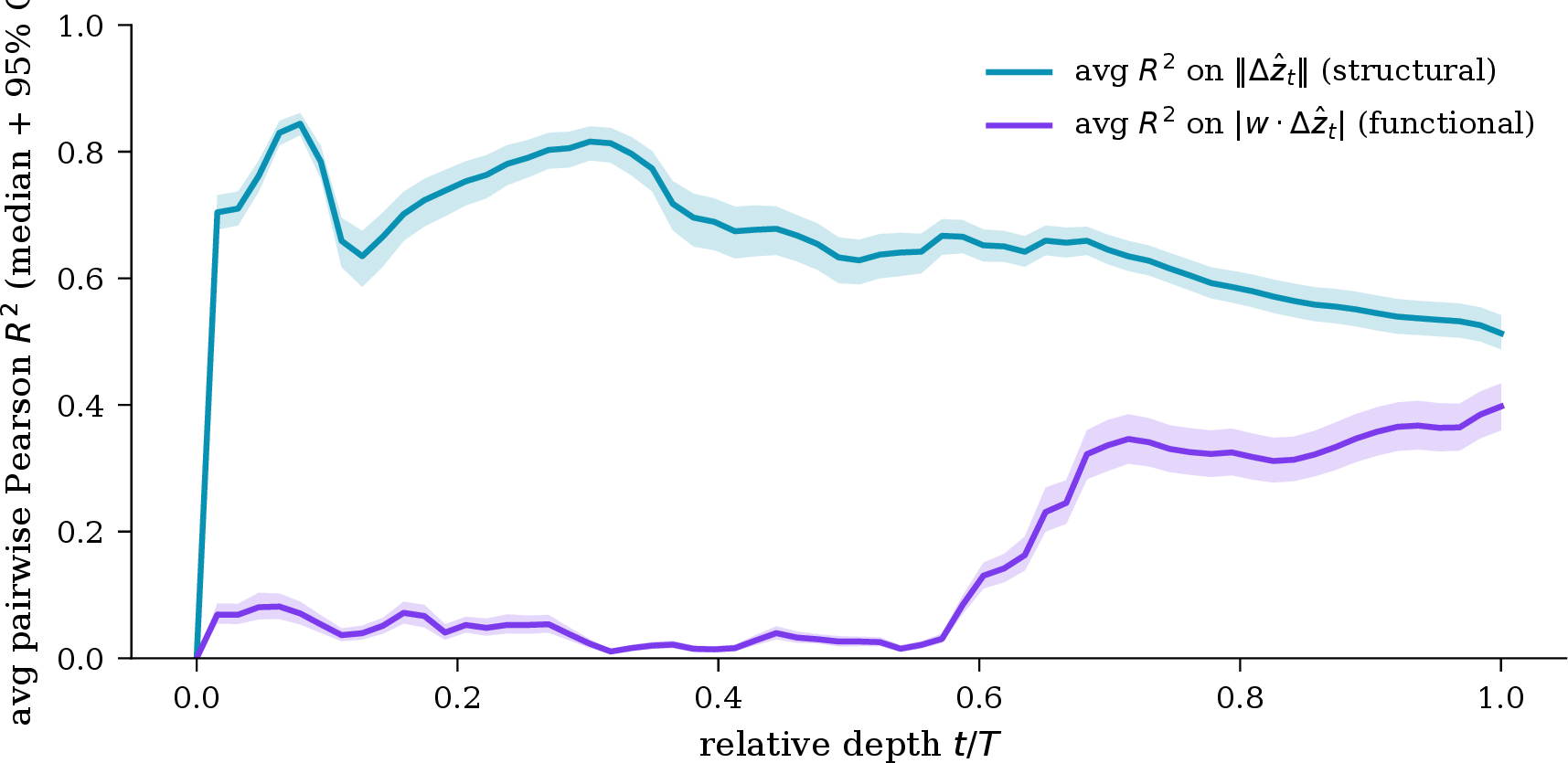
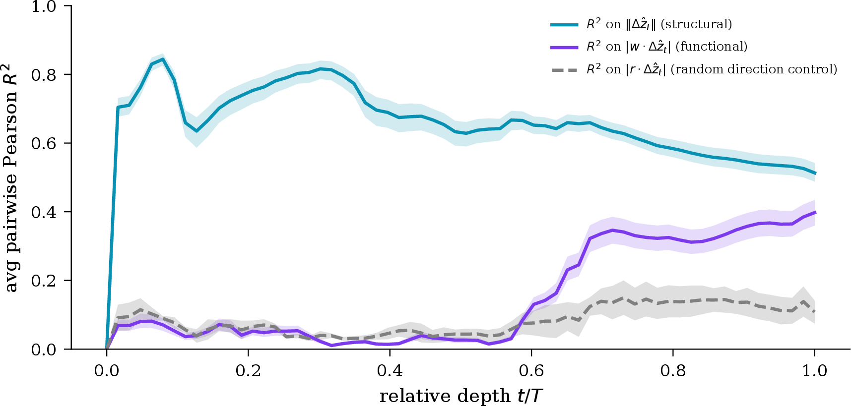
Figure 15: Per-layer correlation analysis with bootstrap confidence intervals and random-direction control.. a — Bootstrap-CI version of 14 (b) (\(B = 500\) resamples of \((\mathrm{\small prompt}, \mathrm{\small segment})\) pairs with replacement; the \(95\%\) CI is the empirical \(2.5\)/\(97.5\) percentile of the pair-averaged \(R^2\) at each depth bin). CIs are \(\leq \pm 0.05\) in \(R^2\) at every depth., b — The structural and functional pair-averaged curves of 15 (a) with the random-direction control overlay (gray dashed). The control rises late too, plateauing at \(R^2 \approx 0.13\)–\(0.15\) before ending at \(R^2 \approx 0.11\) at the readout. The \(v\)-specific premium over the random baseline at the readout is therefore \(\approx 0.29\) in \(R^2\).
[fig:per_layer:pair_average,fig:per_layer:bootstrap] aggregate over the \(10\) model pairs. The headline pattern at this scale is a clean depth dissociation:
Structural agreement \(F_\mathrm{mag}^{(l)}\) is high (\({\sim}0.65\)–\(0.85\)) across most depths past the embedding slot, then tapers to \({\sim}0.51\) at the readout.
Functional agreement \(F_\mathrm{attr}^{(l)}\) is low (\({\lesssim}0.08\)) for the first \(\sim\!55\%\) of depth, rises sharply between depths \(0.55\) and \(0.7\), and reaches \({\sim}0.40\) at the readout.
The final-layer \(F_\mathrm{attr}^{(L)} \approx 0.40\) matches the main-paper \(F_\mathrm{attr}\) baseline (Table 1, BoolQ Open\(\to\)Open) to within sampling noise.
11.3.0.1 Random-direction control.
The dissociation in 15 (a) could in principle be a generic property of late-layer perturbations: any fixed direction in residual-stream space might exhibit a low-then-high cross-model agreement curve. To test this, we replace \(v\) in \(F_\mathrm{attr}^{(l)}\)’s definition with a per-model random unit direction \(r\) matched in norm to \(\|v\|\) (averaging over \(K = 5\) random draws per model on a \(200\)-prompt subsample). 15 (b) overlays the random-direction curve on the structural and functional curves of 15 (a).
The random-direction control rises late as well, plateauing at \(R^2 \approx 0.13\)–\(0.15\) before ending at \(R^2 \approx 0.11\) at the readout — a non-negligible but minority fraction of the headline \(F_\mathrm{attr}^{(L)} \approx 0.40\). The \(v\)-specific premium over the random baseline at the readout layer is therefore \(\approx 0.29\) in \(R^2\). We read this as a partial qualification of the framework’s main-text claim that low \(F_\mathrm{attr}\) reflects models “disagreeing on which inputs drive their predictions”: of the cross-model agreement that \(F_\mathrm{attr}\) measures at the readout, roughly three quarters is \(v\)-specific (i.e., genuinely about the readout direction) and roughly one quarter is direction-agnostic late-stage residual-stream consistency.
11.4 Caveats and scope↩︎
The per-layer extension inherits the assumptions of [sec:preliminaries] [sec:method] but adds three of its own. (i) The logit-lens convention applies \(\mathcal{N}\) at every depth even though intermediate layers are not trained to be readable through \((\mathcal{N}, W_U)\); the cross-model curves in this section should therefore be read as comparing models under a shared reading convention rather than as a claim about each model’s “internal predictions” at intermediate layers. A tuned-lens robustness check [56] is straightforward to add but was not prioritized — the random-direction control (11.3) is more diagnostic for the headline because it directly tests whether the late-rise pattern is \(v\)-specific. (ii) We use single-token \(\mathrm{\small pos}\)/\(\mathrm{\small neg}\) labels so the linearization \(\ell^{(l)} = \mathcal{N}(z^{(l)}) \cdot v\) holds exactly modulo bf16 noise; under the multi-token aggregation used for the main-paper \(F_\mathrm{pred}\)/\(F_\mathrm{attr}\) the projection-based identity becomes a softmax-weighted approximation, which changes both calibration and absolute scales. (iii) Our regex sentence segmenter produces fewer segments per BoolQ passage than the production sentence-tokenizer used in 4; the \(F_\mathrm{attr}^{(L)}\) baseline we measure here (\(\approx 0.40\)) is consistent with the main-text Open\(\to\)Open \(F_\mathrm{attr}\) baseline within sampling noise, but absolute counts of \((\mathrm{\small prompt}, \mathrm{\small segment})\) pairs are not directly comparable. None of these caveats affects the qualitative shape of the depth dissociation, which is robust under all controls in 15 (a) 15 (b).
12 Confidence stratification↩︎
The fidelity metrics reported in 1 aggregate over all prompts in a benchmark. However, prompts vary widely in difficulty: on BoolQ, model log-odds range from \(|\ell| < 0.5\) (near-chance) to \(|\ell| > 30\) (near-certain). We ask whether surrogate fidelity varies systematically with model confidence, operationalized as \(|\ell|\).
12.1 Fidelity versus confidence↩︎
We bin BoolQ prompts into five quintiles by mean \(|\ell|\) across the four Qwen instruct models and compute \(F_\mathrm{pred}\), \(F_\mathrm{attr}\), and \(F_\text{attn}\) within each bin. 16 shows the result.

Prediction fidelity rises from \(F_\mathrm{pred}= 0.03\) in the lowest-confidence quintile to \(0.75\) in the highest—a \(>20\times\) increase. Attribution fidelity follows a similar trajectory, climbing from \(F_\mathrm{attr}= 0.27\) to \(0.61\) (\(+129\%\)). By contrast, attention fidelity is invariant to confidence: \(F_\text{attn} = 0.958 \pm 0.001\) across all five bins.
The strong confidence dependence of \(F_\mathrm{pred}\) carries a practical implication: when models are confident about a prompt, the surrogate’s prediction is a reliable proxy for the target’s (\(F_\mathrm{pred}= 0.75\) in the top quintile). For uncertain prompts, however, surrogate predictions are substantially less trustworthy (\(F_\mathrm{pred}= 0.03\)).
The confidence dependence of \(F_\mathrm{attr}\) has a natural mechanistic explanation. Low-confidence prompts produce small log-odds, and ablating a sentence from such a prompt yields a correspondingly small change in log-odds. When most attribution values in a prompt are near zero, the rank ordering among them is dominated by noise rather than signal, deflating \(R^2\). This is the same near-zero concentration effect noted in 5.2: high-confidence prompts have larger, more discriminative attribution vectors on which models can meaningfully agree.
The flatness of \(F_\text{attn}\) reinforces the dissociation identified in 5.3: attention agreement reflects architectural similarity rather than decision-level consensus, and is therefore insensitive to whether the model finds a prompt easy or hard.
12.2 Whose confidence?↩︎
The previous analysis stratifies by the mean confidence across all four Qwen models. A practitioner may instead want to condition on a single model’s confidence—for instance, the target’s (to assess when a surrogate’s explanations are trustworthy for a given target) or the surrogate’s (to decide whether a particular surrogate prediction merits further analysis). 17 compares these choices.

For both \(F_\mathrm{pred}\) and \(F_\mathrm{attr}\), the fidelity-versus-confidence slope is qualitatively similar regardless of whether we stratify by the smallest model (Qwen-0.5B), the largest (Qwen-14B), or the mean. This is unsurprising in retrospect: because \(F_\mathrm{pred}\) is itself moderate to high within the Qwen family, a prompt that one model finds easy tends to be easy for the others as well. For \(F_\text{attn}\), no stratification produces any gradient, consistent with attention’s insensitivity to prompt difficulty.
Taken together, these results indicate that a practitioner can cheaply screen prompts for surrogate reliability using any available model’s \(|\ell|\) as a proxy for confidence: prompts in the top quintile (\(|\ell| \gtrsim 10\) for Qwen-14B) yield \(F_\mathrm{attr}\approx 0.61\), while prompts in the bottom quintile (\(|\ell| \lesssim 2\)) yield \(F_\mathrm{attr}\approx 0.27\). The output–behavior gap narrows substantially when conditioned on model confidence: at the high-confidence end the gap between prediction and attribution fidelity is \((0.75, 0.61)\), compared to \((0.03, 0.27)\) at the low end.
13 Directional asymmetry via NRMSE↩︎
The agreement metrics used in the main text—Spearman \(\rho\) and Pearson \(R^2\)—are symmetric: swapping which model is called “surrogate” and which is called “target” leaves the statistic unchanged. This symmetry is desirable for summarizing overall agreement, but it cannot detect directional asymmetry: the possibility that using a small model as a surrogate for a large one is systematically worse (or better) than the reverse.
To test for directional effects we introduce normalized root-mean-square error (NRMSE), defined for a surrogate \(s\) predicting a target \(t\) as \[\mathrm{NRMSE}(s \to t) \;=\; \frac{\mathrm{RMSE}(s, t)}{\sigma(y_t)}, \label{eq:nrmse}\tag{15}\] where \(y_t\) is the vector of ground-truth values from model \(t\) and \(\sigma(y_t)\) is its standard deviation. The denominator normalizes the error by the spread of the truth: \(\mathrm{NRMSE} < 1\) means the surrogate is more accurate than the naïve baseline of always predicting \(\bar{y}_t\) (the mean of the target), while \(\mathrm{NRMSE} > 1\) means it is worse.
Because \(\sigma(y_t)\) depends on which model is treated as truth, \(\mathrm{NRMSE}(s \to t) \neq \mathrm{NRMSE}(t \to s)\) in general—even though \(\mathrm{RMSE}(s, t) = \mathrm{RMSE}(t, s)\) is symmetric. This asymmetry reveals which direction of surrogacy is more reliable: if both directions yield low NRMSE, surrogacy is bidirectional; if one direction is high while the reverse is low, the asymmetry identifies the problematic direction. In our data, \(\mathrm{NRMSE}(0.5\text{B} \to 14\text{B}) = 15.2\) while \(\mathrm{NRMSE}(14\text{B} \to 0.5\text{B}) \approx 1.0\)—the small model’s predictions deviate from the 14B model’s outputs by \(15\times\) its own standard deviation, indicating systematic failure rather than mere noise. Thus, a high \(\mathrm{NRMSE}(s \to t)\) flags that model \(s\) is an unreliable surrogate for model \(t\), even when the symmetric Spearman \(\rho\) between them appears moderate.
We restrict this analysis to \(F_\mathrm{pred}\) and \(F_\mathrm{attr}\); raw attention magnitudes differ by up to \(10{,}000\times\) across model sizes, causing NRMSE to explode to \({\sim}100{,}000\) for some pairs—a scale artifact rather than a meaningful directional difference.
18 shows \(4 \times 4\) NRMSE heatmaps for \(F_\mathrm{pred}\) and \(F_\mathrm{attr}\) across the Qwen 2.5 instruct family (0.5B, 3B, 7B, 14B), with rows indexing the surrogate and columns indexing the target.
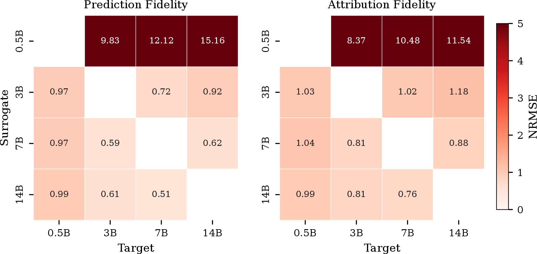
The heatmaps reveal a sharp qualitative boundary at 3B parameters. For \(F_\mathrm{pred}\), \(\mathrm{NRMSE}(0.5\text{B} \to 14\text{B}) = 15.2\)—catastrophically worse than the mean baseline—while the reverse gives \(\mathrm{NRMSE} \approx 1.0\). \(F_\mathrm{attr}\) follows the same pattern: \(11.5\) versus \({\approx}\,1.0\). Among the three larger models (3B, 7B, 14B), NRMSE is below 1.0 in most directions for both metrics, indicating that surrogacy is approximately symmetric and consistently better than the mean baseline. The practical implication is that directional asymmetry is a concern only when the surrogate is substantially smaller than the target—specifically, below the \({\sim}3\)B threshold identified in the main text—and that above this threshold a practitioner can treat surrogacy as approximately bidirectional.
14 Representation fidelity decomposition↩︎
As shown in 6 , the attribution \(\Delta \ell = \lVert \Delta z \rVert \, \lVert v \rVert \, \cos(\Delta z, v)\) decomposes into a perturbation magnitude and an alignment term. The representation-level metrics \(F_\mathrm{mag}\) and \(F_\mathrm{align}\) (10 11 ) measure cross-model agreement on each factor separately. Here we examine how the gap between these two sub-metrics explains the low \(F_\mathrm{attr}\) observed in the main text.
19 shows a \(5 \times 5\) split heatmap of \(F_\mathrm{mag}\) and \(F_\mathrm{align}\) across the five open models on BoolQ.

\(F_\mathrm{mag}\) is uniformly high: even the weakest pair (Qwen-0.5B \(\leftrightarrow\) Qwen-7B, \(R^2 = 0.641\)) exceeds \(F_\mathrm{attr}\) by a wide margin. Cross-family agreement (Llama-8B vs.any Qwen model) is comparably strong (\(F_\mathrm{mag}\geq 0.768\)), indicating that perturbation magnitude is largely architecture-independent.
\(F_\mathrm{align}\) is substantially lower (mean \(0.17\), range \(0.058\)–\(0.294\)). The gap between \(F_\mathrm{mag}\) and \(F_\mathrm{align}\) identifies the bottleneck for attribution fidelity: models agree that ablating a given segment causes a large representational shift, but disagree on how much that shift projects onto the readout direction \(v\). Because \(\gamma = \cos(\Delta z, v)\) depends on each model’s readout direction—which encodes how the model distinguishes positive from negative classes in representation space—low \(F_\mathrm{align}\) indicates that different models have learned fundamentally different internal geometries for the same binary classification task.
This decomposition clarifies the hierarchy of fidelity observed in the main text:
\(F_\text{attn} \approx 0.96\): models attend to the same tokens.
\(F_\mathrm{mag}\approx 0.81\): ablating a segment perturbs representations by a similar amount across models.
\(F_\mathrm{align}\approx 0.17\): models encode the task along different readout directions, so the same perturbation projects differently onto each model’s decision axis.
\(F_\mathrm{attr}\approx 0.33\): the causal effect on the output disagrees (a joint consequence of \(F_\mathrm{mag}\) and \(F_\mathrm{align}\)).
The practical implication is that the “output–behavior gap” (\(F_\mathrm{pred}\gg F_\mathrm{attr}\)) is not because models disagree about which segments are structurally important—they largely do agree, as \(F_\mathrm{mag}\) shows—but because each model’s decision axis differs. A surrogate’s attribution ranking is unreliable not because it fails to detect the right perturbations, but because the direction along which perturbations translate into output changes is model-specific.
15 System-prompt perturbation as a secondary behavioral fidelity signal↩︎
The behavioral fidelity framework introduced in Section 3 measures attribution via input ablation: removing a segment of the prompt and observing the change in log-odds. We now consider an orthogonal causal intervention: mutate the system prompt, and ask whether models that respond similarly to context perturbation also exhibit greater surrogate fidelity. Where ablation measures sensitivity to the absence of information, system-prompt perturbation measures sensitivity to its framing.
Concretely, we use GEPA [57], a state-of-the-art prompt optimization algorithm, both as a method for generating a diverse set of system-prompt candidates and as a tool for per-model optimization. This enables us to assess two strict tests of context-level fidelity: (i) perturbation-response similarity: do models whose predictions shift in correlated ways under the same system-prompt variation constitute better surrogates for one another? (ii) prompt transferability: does a system prompt optimized with respect to donor model \(M_D\) improve performance when applied to recipient model \(M_R\), and does the degree of transfer serve as a directional surrogacy measure in contrast to the similarity metrics of Section 3?
15.0.0.1 Experimental protocol.
We evaluate the same eleven models, spanning four families (Qwen, Llama, GPT, Gemini), described in Section 4.3 on the ANLI R3 test split (\(n=400\)), chosen for its difficulty to ensure headroom for prompt-driven gains and reason labels required by GEPA’s feedback mechanism. We construct three prompt conditions: (i) candidates – ten system prompts selected for maximal tree-path diversity from a single GEPA run targeting GPT-4.1 (GPT-5.2 as reflector), applied uniformly to all models as shared context-level perturbations; (ii) per-model best – the top-performing prompt from an independent GEPA run targeting each model individually; and (iii) the baseline system prompt used as the control. All GEPA runs use 20 optimization steps with minibatches of 20 from the ANLI R3 development split.
15.1 Perturbation-response fidelity↩︎
We ask whether replacing the system prompt with a GEPA-generated alternative drives two models’ predictions into alignment, and whether this alignment extends to how those predictions shift. For each prompt condition and model, we compute \(F_\mathrm{pred}\) (Pearson \(R^2\) of log-odds) and \(F_\mathrm{attr}\) (Pearson \(R^2\) of \(\Delta\ell\) relative to the baseline). Table 3 reports the results.
| Condition | All | W. Qwen | W. Qwen- | W. Llama | W. Llama- | W. GPT | Cross | |
|---|---|---|---|---|---|---|---|---|
| \(\Fpred\) | Baseline | .385 | .135 | .278 | .600 | .716 | .838 | .362 |
| Candidates | .480 | .305 | .430 | .602 | .730 | .840 | .469 | |
| Cross-model best | .478 | .297 | .541 | .610 | .816 | .839 | .467 | |
| Per-model best§ | .479 | .303 | .596 | .620 | .808 | .863 | .468 | |
| \(\Fattr\) | Candidates | .092 | .030 | .077 | .204 | .213 | .095 | .080 |
| Cross-model best | .044 | .023 | .062 | .113 | .163 | .000 | .038 | |
| Per-model best§ | .069 | .058 | .058 | .089 | .035 | .033 | .071 |
The prediction-level finding is clear: replacing the baseline system prompt with a more structured alternative increases cross-model prediction agreement. All system prompt condition sets raise \(F_\mathrm{pred}\) by approximately 25% over the baseline. The gain holds across all family groupings and is insensitive to prompt source; even per-model best prompts, where each model is under its own independently optimized prompt, act as a non-uniform perturbation, suggesting that prompt optimization drives models toward a shared output regime independent of perturbation direction.

Attribution fidelity tells a sharply different story. Mean pairwise \(F_\mathrm{attr}\) under diverse candidates is \(R^2 = .092\), comparable to the \(R^2 = .241\) reported for sentence-level input ablation on ANLI R3 (Table 2), and drops further to \(.044\) under cross-model best prompts. The gap between \(F_\mathrm{pred}\) and \(F_\mathrm{attr}\) (\(.480\) vs.\(.092\)) mirrors the output–behavior dissociation observed under input ablation: models that converge on predictions do not converge on how those predictions respond to context perturbation. The dissociation is most pronounced for GPT-4o and GPT-4.1, which achieve the highest \(F_\mathrm{pred}\) in our evaluation (\(R^2 = .840\)) but yet near-zero \(F_\mathrm{attr}\) under diverse candidates (\(.095\)) and effectively zero under cross-model best prompts (\(.000\)). Despite near-perfect agreement on log-odds, prompts that shift one model’s per item predictions do not reliably shift the other’s, exemplifying the critical failure mode identified in Section 5.2: high output fidelity masking divergent causal structure.
15.2 Cross-model prompt transfer↩︎
The bilateral fidelity metrics in Section 15.1 treat prompt perturbation as a shared intervention. We now ask a directed question: can a prompt optimized for one model transfer its behavioral gains to another, and does the degree of transfer serve as a directional surrogacy measure that the symmetric metrics of Section 3 cannot provide?
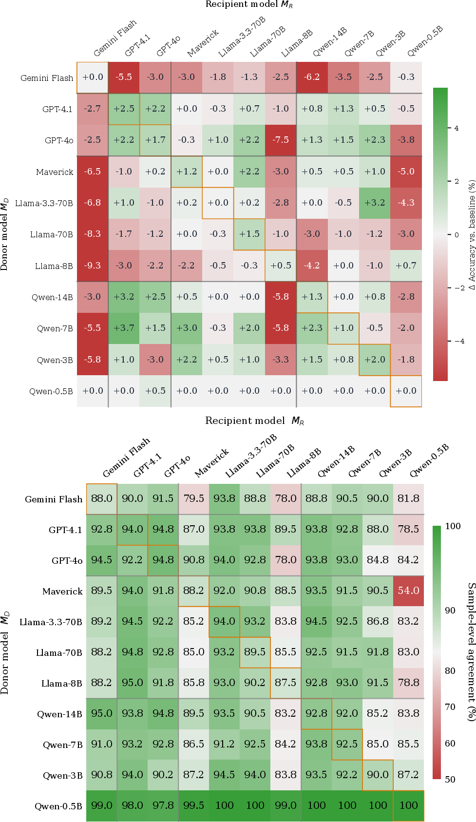
For each donor–recipient pair \((M_D, M_R)\), we apply the system prompt optimized for \(M_D\) to \(M_R\) and measure the accuracy change relative to \(M_R\)’s baseline. Figure 21 (left panel) reports the full \(11 \times 11\) transfer matrix. Cross-model transfer is predominantly neutral or negative (mean off-diagonal \(\Delta\)accuracy \(= -1.4\%\)): prompts that adapt to one model’s failure patterns do not generally remedy another’s. Crucially, the matrix is asymmetric, transferring \(M_D\)’s prompt to \(M_R\) yields a different outcome than the reverse. In line with the small accuracy deltas, sample-level agreement between \(M_R\)’s predictions under \(M_D\)’s optimized prompt and \(M_R\)’s own baseline is high (right panel; off-diagonal mean 90.4%). Optimized prompts largely preserve which samples each model answers correctly, perturbing a minority of per-item decisions. The principal exception is Maverick \(\to\) Qwen-0.5B (54.0%), consistent with Qwen-0.5B’s position as a general outlier (Section 5.1).
15.3 Voice transplant: prompt as directional bias vector↩︎
\(F_\mathrm{pred}\) and \(F_\mathrm{attr}\) measure bilateral similarity: are two models alike? They do not measure whether one model’s behavior can be steered toward another’s. We introduce the voice-transplant correlation to capture this asymmetric notion of surrogacy. For each ordered pair \((M_D, M_R)\), we define \[\mathrm{VT}(M_D \to M_R) = r\!\left(\ell_{M_D}^{\mathrm{baseline}} - \ell_{M_R}^{\mathrm{baseline}},\; \Delta\ell_{M_R}^{\mathrm{best}_{M_D}}\right)\] where \(\ell_{M_D}^{\mathrm{baseline}} - \ell_{M_R}^{\mathrm{baseline}}\) is the natural difference in log-odds output between the donor and recipient under the baseline prompt, and \(\Delta\ell_{M_R}^{\mathrm{best}_{M_D}}\) is the shift in the recipient’s log-odds induced by applying the donor’s optimized prompt. Positive VT indicates the recipient shifts toward the donor; negative VT indicates the recipient shifts away.

Figure 22 reports mean VT received across all non-self donors, ranked by susceptibility. Qwen-14B achieves the highest mean VT (\(r = +0.71\)): applying any other model’s optimized prompt consistently shifts its log-odds toward the donor’s baseline, indicating strong behavioral malleability. Most models demonstrate some degree of positive convergence, GPT-4.1 (\(r = +0.43\)), Qwen-3B (\(r = +0.39\)), Llama-3.3-70B (\(r = +0.38\)), spanning model families and architectures, suggesting that prompt-based alignment is broadly viable. At the other end, Llama-8B (\(r = -0.09\)) and GPT-4o (\(r = -0.004\)) show negligible or negative convergence: applying another model’s optimized prompt does not reliably close the log-odds gap.
15.4 Summary↩︎
System-prompt perturbation replicates the central finding under a complementary form of causal intervention. Perturbing the instructional context drives cross-model output convergence while attribution fidelity remains uniformly low, independent of if the perturbation is a diverse set of candidates, or optimized for each model itself. The dissociation is starkest for GPT-4o and GPT-4.1, which achieve the highest prediction fidelity in our evaluation (0.840) yet near-zero attribution fidelity under every prompt condition tested. Cross-model prompt transfer shows limited success in our evaluation, though the degree and direction of transfer vary across pairs, indicating that prompt-level surrogacy is inherently directional. Finally, we propose voice-transplant (VT) susceptibility as a lightweight, API-accessible measure of a model’s impressionability, its capacity to be behaviorally steered toward a target. This provides MI practitioners a preliminary diagnostic for identifying which surrogates are amenable to prompt-based alignment before committing to mechanistic analysis.
16 Extension to multi-class classification↩︎
The framework of 3 assumes binary classification, where the log-odds \(\ell(x) = \log P(y^+) - \log P(y^-)\) reduce to a single scalar per prompt. We now extend prediction and attribution fidelity to \(K\)-class settings (e.g., \(K=4\) for multiple-choice benchmarks such as RACE), where a single scalar cannot capture the full structure of a model’s prediction.
16.0.0.1 Pairwise log-odds representation.
For a \(K\)-class task with label set \(\mathcal{Y} = {y_1, \ldots, y_K}\), we represent each model’s prediction as the vector of all \(\binom{K}{2}\) pairwise log-odds: \[\boldsymbol{\ell}(x) = \bigl(\log P(y_a \mid x) - \log P(y_b \mid x)\bigr)_{(a,b) \in \mathcal{C}}, \label{eq:pairwise95logodds}\tag{16}\] where \(\mathcal{C} = {(a, b) : 1 \le a < b \le K}\). For a 4-class task, this yields a 6-dimensional vector per prompt.
This representation has two desirable properties. First, it is label-free: no knowledge of the correct answer is required, since all class pairs are included symmetrically. Second, pairwise log-odds are invariant to the softmax normalization constant \(C\) (1 ), so they isolate relative preferences among the valid options and are unaffected by how much probability mass a model places on non-option tokens. The binary case is recovered exactly: when \(K = 2\), \(\binom{2}{2} = 1\) and \(\boldsymbol{\ell}(x)\) reduces to the scalar \(\ell(x)\) of 2 .
16.0.0.2 Ablation in the multi-class setting.
Under leave-one-out ablation, each segment removal changes the prediction vector from \(\boldsymbol{\ell}(x)\) to \(\boldsymbol{\ell}(x_{\setminus i})\). The vector-valued ablation response is: \[\boldsymbol{\Delta\ell}i(x) = \boldsymbol{\ell}(x) - \boldsymbol{\ell}(x{\setminus i}) \in \mathbb{R}^{\binom{K}{2}}, \label{eq:multiclass95attribution}\tag{17}\] which captures how removing segment \(i\) shifts the relative preference between every class pair simultaneously.
16.0.0.3 RV coefficient.
To measure agreement between two models’ vector-valued predictions or attributions, we require a multivariate extension of correlation. We use the RV coefficient [5], which measures the closeness of two data matrices in the Hilbert–Schmidt inner product space.
For two centered data matrices \(\mathbf{X}, \mathbf{Y} \in \mathbb{R}^{n \times p}\) (where \(n\) is the number of observations and \(p = \binom{K}{2}\)), the RV coefficient is: \[\mathrm{RV}(\mathbf{X}, \mathbf{Y}) = \frac{\operatorname{tr}\!\left(\mathbf{X}^\top \mathbf{Y} , \mathbf{Y}^\top \mathbf{X}\right)}{\sqrt{\operatorname{tr}\!\left(\mathbf{X}^\top \mathbf{X} , \mathbf{X}^\top \mathbf{X}\right) \cdot \operatorname{tr}\!\left(\mathbf{Y}^\top \mathbf{Y} , \mathbf{Y}^\top \mathbf{Y}\right)}}. \label{eq:rv}\tag{18}\] The RV coefficient ranges from 0 (no agreement) to 1 (proportional matrices). When \(p = 1\), it reduces to the squared Pearson correlation \(R^2\).
16.0.0.4 Multi-class fidelity metrics.
Prediction and attribution fidelity extend using the pairwise log-odds vectors and RV: \[\begin{align} F_\text{pred}(M_S, M_T; \mathcal{D}) &= \mathrm{RV}\!\left( \boldsymbol{L}_{M_S}, \boldsymbol{L}_{M_T} \right), \tag{19} \\ F_\text{attr}(M_S, M_T; \mathcal{D}) &= \mathrm{RV}\!\left( \boldsymbol{\Delta L}_{M_S}, \boldsymbol{\Delta L}_{M_T} \right), \tag{20} \end{align}\] where \(\boldsymbol{L}_M \in \mathbb{R}^{|\mathcal{D}| \times \binom{K}{2}}\) stacks the per-prompt prediction vectors, and \(\boldsymbol{\Delta L}_M \in \mathbb{R}^{N \times \binom{K}{2}}\) stacks all segment-level ablation response vectors globally across all prompts (\(N = \sum{x} N_x\), where \(N_x\) is the number of segments in prompt \(x\)).
Both metrics compute the RV coefficient on the full data matrices globally. This parallels the binary case, where \(F_\text{pred}\) and \(F_\text{attr}\) are global correlations across all prompts or (prompt, segment) pairs respectively.
16.1 Demonstrative experiment: RACE↩︎
We evaluate multi-class fidelity on RACE [11], a 4-way multiple-choice reading comprehension benchmark with 4,934 test prompts. Each prompt consists of a multi-paragraph article followed by a question with four options (A–D), making it well-suited for sentence-level ablation: passages contain 8–10 sentences on average.
16.1.0.1 Results.
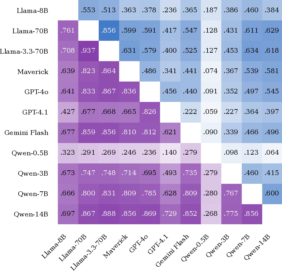
We score 11 models spanning four families: Qwen2.5, and Llama-3/4, GPT and Gemini. 23 shows \(11 \times 11\) pairwise heatmaps of \(F_\text{pred}\) and \(F_\text{attr}\) on RACE. Comparing this to the heatmap in 3, which is evaluated on the binary dataset of BoolQ, the relative model fidelities of both prediction and attribution are well aligned between these two datasets.
17 Connection to representational similarity↩︎
The progression from binary log-odds to multi-class pairwise log-odds suggests a deeper perspective: our fidelity metrics are task-relevant projections of a full representational similarity measure, while accessible through log-probabilities alone.
17.0.0.1 From scalars to vectors to representations.
In the binary case, prediction fidelity compares the scalar log-odds \(\ell(x) = z \cdot v\) across prompts, where \(v = u_+ - u_-\) is the log-odds direction (2 ). This is a projection of the residual stream \(z \in \mathbb{R}^d\) onto a single direction in representation space. In the multi-class case (16), the pairwise log-odds vector \(\boldsymbol{\ell}(x) \in \mathbb{R}^{\binom{K}{2}}\) corresponds to projecting \(z\) onto \(\binom{K}{2}\) directions simultaneously: \[\ell_{ab}(x) = z \cdot (u_a - u_b), \qquad (a, b) \in \mathcal{C}, \label{eq:projection}\tag{21}\] where \(u_a, u_b\) are columns of the unembedding matrix \(W_U\). Stacking these projections, the full pairwise log-odds vector is \(\boldsymbol{\ell}(x) = Pz\), where \(P \in \mathbb{R}^{\binom{K}{2} \times d}\).
The same applies to attributions: the vector-valued ablation response \(\boldsymbol{\Delta\ell}_i(x) = P\Delta z_i\) (17 ) is the projection of the representation perturbation \(\Delta z_i = z - z'_i\) onto the same task-relevant subspace.
At the limit, one could skip the projection entirely and compare the full residual-stream matrices \(\mathbf{Z}_M \in \mathbb{R}^{n \times d}\) directly. This requires white-box access to model internals, but yields a complete picture of representational similarity.
17.0.0.2 Centered Kernel Alignment.
The natural measure for comparing full representation matrices is Centered Kernel Alignment (CKA) [6], which has become the standard for comparing neural network representations across architectures. For centered data matrices \(\mathbf{X}, \mathbf{Y} \in \mathbb{R}^{n \times d}\), linear CKA is defined as: \[\text{CKA}(\mathbf{X}, \mathbf{Y}) = \frac{\operatorname{tr}\!\left(\mathbf{X}\mathbf{X}^\top \mathbf{Y}\mathbf{Y}^\top\right)}{\sqrt{\operatorname{tr}\!\left((\mathbf{X}\mathbf{X}^\top)^2\right) \cdot \operatorname{tr}\!\left((\mathbf{Y}\mathbf{Y}^\top)^2\right)}}. \label{eq:cka}\tag{22}\] This is the cosine similarity between the two models’ Gram matrices \(\mathbf{X}\mathbf{X}^\top\) and \(\mathbf{Y}\mathbf{Y}^\top\) in the Hilbert–Schmidt inner product space. Each Gram matrix entry \((\mathbf{X}\mathbf{X}^\top)_{ij} = x_i \cdot x_j\) captures the dot-product similarity between two prompts’ representations within a model; CKA asks whether these pairwise similarity structures agree across models.

Linear CKA is mathematically equivalent to the RV coefficient. When applied to scalar data (\(d = 1\)), it reduces to the squared Pearson correlation \(r^2\) — which is the binary prediction fidelity metric \(F_\text{pred}\) of 8 . The RV coefficient (18 ) applied to multi-class pairwise log-odds is therefore CKA on the projected representations \(P\mathbf{Z}\). Our fidelity framework forms a unified hierarchy: \[\underbrace{r^2(\ell_{M_S}, \ell_{M_T})}_{\text{binary } F\text{pred}} \subset \underbrace{\text{RV}(\boldsymbol{L}_{M_S}, \boldsymbol{L}_{M_T})}_{\text{multi-class } F\text{pred}} \subset \underbrace{\text{CKA}(\mathbf{Z}_{M_S}, \mathbf{Z}_{M_T})}_{\text{representational similarity}} \label{eq:hierarchy}\tag{23}\] Each level projects the residual stream onto progressively fewer task-relevant directions: \(d\) (full representation), \(\binom{K}{2}\) (pairwise log-odds), or \(1\) (binary log-odds).
17.0.0.3 Task-relevant projections vs.random projections.
Our projections are not arbitrary — they use the unembedding directions \((u_a - u_b)\) that the model was trained to separate. The training objective (next-token prediction) optimizes the residual stream \(z\) so that its projection onto unembedding vectors produces the correct probability distribution. These directions therefore capture maximal task-relevant variance in \(z\) by construction.
By contrast, the Johnson–Lindenstrauss lemma [58] guarantees that random projections from \(\mathbb{R}^d\) to \(\mathbb{R}^k\) preserve pairwise dot products up to \((1 \pm \varepsilon)\) distortion when \(k \geq O(\log n / \varepsilon^2)\). For \(n = 5{,}000\) prompts and \(\varepsilon = 0.1\), this requires \(k \approx 850\) random dimensions to approximate the full Gram matrix. Our task-relevant projections use only \(k = \binom{K}{2}\) directions (6 for a 4-class task) yet capture the subspace that determines the classification output, i.e., the operationally relevant subspace for surrogate fidelity.
This perspective also clarifies the practical value of our fidelity framework: it provides a window into representational similarity through black-box API access. Full CKA requires white-box access to hidden states; our projected variant requires only log-probabilities for the related tokens.

17.0.0.4 Projected vs.full representational CKA.
To validate that our log-odds fidelity metrics are faithful proxies for representational similarity, we compute both full CKA on the residual stream \(z\) and \(r^2\) on binary log-odds on BoolQ for all pairs of open-source models (Qwen2.5-0.5B, 3B, 7B, 14B-Instruct and Llama-3.1-8B, yielding 10 model pairs). This is done for both prediction and attribution fidelity. 24 shows the correlation between the two measures across model pairs.
17.0.0.5 Convergence of random projections.
To quantify the efficiency of task-relevant projections, we compare three projection strategies as a function of projection dimension \(n\) from \(n = 1\) over \(n = d\) (the model’s latent dimension):
Random Gaussian: project \(z\) onto \(n\) i.i.d.random unit vectors.
Unembeddings coupled: project \(z\) onto \(n\) randomly sampled tokens unembeddings (same token for \(M_S\) and \(M_T\)).
Unembeddings uncoupled: project \(z\) onto \(n\) randomly sampled tokens unembeddings (independent tokens for \(M_S\) and \(M_T\)).
For each \(n\) and each strategy, we compute RV on the \(n\)-dimensional projected data and track convergence toward full CKA. 25 shows convergence curves of different model pairs. From the plots, we can see coupled unembeddings usually converge a little faster, but to a lower plateau, while only random projection can reach CKA-like levels. This aligns with our expectation that the unembeddings capture a much more relevant subspace, which is effective but limited in covering the whole representation space.
Comparing with the \(R^2\) fidelity values shown in 3, we can see the heatmap’s numbers are much higher than the corresponding model pairs’ curve at the same dimension \(d = 1\). This shows our task-relevant log-odds is an effective approach to estimate models’ representational agreement.
References↩︎
Our framework is intervention-agnostic. For our experiments, we use prompt-level leave-one-out ablations because they are compatible with black-box API access.↩︎
For RMSNorm (used in Qwen 2.5 and Llama 3), \(f(\hat{z}) = \|\hat{z}\|/\sqrt{d}\).↩︎
We restrict the per-layer extension to single-token positive/negative labels so that the linearization \(\ell = z \cdot v\) from 2 holds exactly modulo bit-precision noise, allowing \(\ell^{(l)}\) to be read directly from \(\mathcal{N}(z^{(l)})\) without instantiating \(W_U\) at every layer. We verified this identity on Qwen-0.5B for all \(L = 24\) decoder layers: the maximum discrepancy between \(\mathcal{N}(z^{(l)}) \cdot v\) and the explicit \(W_U[\mathrm{\small pos}] - W_U[\mathrm{\small neg}]\) projection of \(\mathcal{N}(z^{(l)})\) is \(9.6 \times 10^{-2}\) versus a five-bf16-ULP threshold of \(2.4 \times 10^{-1}\). The analogous DLA-decomposition identity from 4 holds to \(8.6 \times 10^{-2}\).↩︎