Spatially Coupled MacKay–Neal/Hsu–Anastasopoulos CSS Codes Achieve the Quantum-Erasure Hashing Bound by Seeded BP Decoding
June 30, 2026
Abstract
In classical sparse-graph coding, spatial coupling is a mechanism by which belief-propagation (BP) decoding attains the maximum-a-posteriori (MAP) or area-threshold performance of the uncoupled system. Since MacKay–Neal/Hsu–Anastasopoulos (MN/HA) punctured sparse ensembles achieve capacity under MAP decoding, it is natural to ask whether spatially coupled MN/HA-type Calderbank–Shor–Steane (CSS) codes can reach the hashing bound on the quantum erasure channel under seeded BP decoding. We answer this question at the density evolution (DE) level for hard-erasure CSS decoding. On an erased coordinate, the two binary Pauli components remain unresolved, equivalently the erased qubit is represented by the four Pauli possibilities. We first define the CSS ensemble through sparse punctured matrices and the corresponding dense parity-check matrices. For fixed finite Z-side, X-side, and check degrees, we then derive a five-message uncoupled DE recursion, decompose it into Z-side and X-side constituent systems, and define the two constituent potentials. Applying the coupled-vector potential method to the two constituents separately proves that seeded BP decoding on the resulting finite-degree factor graphs reaches the smaller of the Z-side degree ratio and the X-side complementary degree ratio. In the X/Z equal-rate specialization, where the Z-side and X-side constituent design rates are equal, this BP threshold is the hashing-bound channel parameter determined by the design rate. Thus the paper gives a DE-level proof that seeded BP decoding with finite-degree factor graphs achieves the hashing bound for the X/Z equal-rate family. Finite-length BP concentration, block-error convergence, and a finite-code realization of the ideal DE seed are separate questions.
1 Introduction↩︎
Calderbank–Shor–Steane (CSS) codes are a standard way to build quantum stabilizer codes from an orthogonality relation between two classical linear codes [1], [2]. On the classical side, low-density parity-check (LDPC) codes make local graph-based decoding possible [3], [4]. The MacKay–Neal (MN) and Hsu–Anastasopoulos (HA) ensembles use punctured sparse representations to obtain bounded-degree graphical constructions with capacity-oriented decoding properties [5], [6].
Quantum LDPC code construction has developed in parallel with the classical sparse-graph coding literature. Hypergraph-product codes gave positive-rate quantum LDPC families with distance proportional to the square root of the block length [7], and lifted-product constructions later gave asymptotically good quantum LDPC codes [8]. Spatial coupling has also been studied directly for quantum LDPC codes, including spatially coupled quasi-cyclic quantum LDPC codes, entanglement-assisted spatially coupled quantum LDPC codes, and algebraic spatially coupled quantum LDPC constructions [9]–[11]. These construction results motivate decoding analyses for CSS codes, but they do not by themselves provide a density-evolution (DE) theorem for the punctured MN/HA representation considered here.
Before the terminology of spatial coupling became standard, the same construction principle appeared in the study of low-density parity-check (LDPC) convolutional codes: periodic low-density convolutional parity-check matrices were introduced in [12], and terminated LDPC convolutional ensembles were shown by density evolution to have belief-propagation (BP) thresholds close to capacity in [13], [14]. Protograph-based LDPC convolutional and spatially coupled LDPC ensembles were then developed as a structured design framework with distance and threshold analysis [15], [16]. Spatial coupling was also formulated in the classical LDPC setting as a method that lets BP decoding attain the maximum-a-posteriori (MAP) or area-threshold performance of the uncoupled system [17]. The vector-potential method extends the same proof strategy to DE systems with multiple message types [18]. For MN/HA-type ensembles, prior work proceeds from threshold improvement and asymptotic analysis on the binary erasure channel (BEC), to capacity-achieving bounded-degree cases, to symmetric-information-rate (SIR) achievability over generalized erasure channels (GECs) [19]–[23]. Thus, from the classical viewpoint, the natural expectation is that spatial coupling should expose the MAP performance of MN/HA-type systems to BP decoding.
This expectation has a direct CSS analogue. If the Z-side and X-side MN/HA constituents have MAP thresholds matching their respective capacity or area limits, then using those constituents in a CSS sparse representation suggests that spatial coupling should make seeded BP decoding reach the quantum-erasure hashing-bound parameter. The point is not that the conclusion follows automatically from the classical results: the erased quantum coordinate couples the two Pauli components and produces the five-message recursion studied below. The role of this paper is to prove the corresponding threshold-saturation statement for that recursion.
The finite-degree CSS construction in [24] uses MN/HA-type punctured sparse representations as nested structures for building CSS pairs. Its minimum-distance result is an existence statement for the finite random code ensemble: with suitable finite degrees, the resulting CSS codes have positive relative minimum distance, and the achievable rate–distance tradeoff reaches the quantum Gilbert–Varshamov benchmark. This distance statement controls the code family itself, but it does not specify an iterative erasure decoder or its threshold. This paper isolates the hard-erasure decoding problem associated with the same sparse representation over the quantum erasure channel. On erased coordinates, the two Pauli components remain unresolved, so the Z-side and X-side sparse decoding problems are described by a five-message recursion driven by the same erasure probability.
The contribution of this paper is to formulate and prove the MN/HA spatial-coupling potential analysis for that five-message recursion. We state the uncoupled recursion, decompose it into two constituent recursions, express the hashing bound by a degree-of-freedom count, and prove saturation of seeded spatial coupling as a deterministic DE statement.
2 Sparse CSS Erasure Models↩︎
This section first fixes the CSS notation and the quantum-erasure decoding model, and then defines the ensemble through punctured sparse representations. We begin by briefly reviewing the finite-degree CSS construction of [24], keeping only the notation needed for the later decoding analysis. All vectors are column vectors, and \(\boldsymbol{0}\) denotes the zero column vector of the context-dependent length. We write \(\operatorname{Row}(M)\) for the row span of \(M\), represented as a subspace of column vectors.
Start from a general CSS code specified by two binary check matrices \[H_X\in\mathbb{F}_2^{m_X\times N},\qquad H_Z\in\mathbb{F}_2^{m_Z\times N},\qquad H_XH_Z^T=\boldsymbol{0}.\] Rows of \(H_X\) are interpreted as X-type stabilizers, and rows of \(H_Z\) as Z-type stabilizers. Write a binary Pauli error as \((\boldsymbol{e}_X,\boldsymbol{e}_Z)\in\mathbb{F}_2^N\times\mathbb{F}_2^N\). The measured syndromes are \[\boldsymbol{\sigma}_X=H_X\boldsymbol{e}_Z,\qquad \boldsymbol{\sigma}_Z=H_Z\boldsymbol{e}_X .\]
The decoder is given the erasure state \(S=(S_1,\ldots,S_N)\). If \(S_i=0\), the coordinate is known and \((e_{X,i},e_{Z,i})=(0,0)\). If \(S_i=1\), the erased coordinate leaves \(e_{X,i}\) and \(e_{Z,i}\) unresolved; equivalently, the erased qubit is represented by the four possibilities \(I,X,Y,Z\). Quantum-erasure decoding has been studied for surface codes, color codes, hypergraph product codes, and more general quantum LDPC codes using linear-time maximum-likelihood decoding, trimming, fast erasure decoding, belief propagation with guided decimation, cluster decomposition, degeneracy-aware BP, stabilizer-assisted inactivation, and quantum Maxwell erasure decoding [25]–[32]. The deterministic density-evolution recursion associated with this model is introduced in 3.
The decoding objective is to recover an estimate \((\widehat{\boldsymbol{e}}_X,\widehat{\boldsymbol{e}}_Z)\) from \((\boldsymbol{\sigma}_X,\boldsymbol{\sigma}_Z)\) and \(S\) with the same syndrome, such that the residual is CSS-stabilizer equivalent to the true error: \[\widehat{\boldsymbol{e}}_X+\boldsymbol{e}_X\in\operatorname{Row}(H_X),\qquad \widehat{\boldsymbol{e}}_Z+\boldsymbol{e}_Z\in\operatorname{Row}(H_Z).\] For a hard-erasure decoder in these models, the basic state is whether the relevant visible component has been resolved or remains unknown. Here and throughout the paper, a visible component means an unpunctured component that remains as a physical CSS coordinate, in contrast to the hidden auxiliary components that are punctured in the sparse representation.
The next definitions fix the random matrix ensembles used in the sparse representation. We state both the uncoupled and tail-biting spatially coupled versions so that the finite ensembles are specified independently of any decoding dynamics.
Definition 1 (\((j,k,M)\)-regular random matrix). Let \(j,k,M\) be positive integers such that \(k\) divides \(jM\), and put \(m=jM/k\). A \((j,k,M)\)-regular random matrix is a binary matrix \[A\in\mathbb{F}_2^{m\times M}\] drawn uniformly from the set of matrices with every column of weight \(j\) and every row of weight \(k\). Equivalently, it is the regular specialization of the standard socket ensemble \(\mathrm{LDPC}(\Lambda,P)\) in [4], with \(M\) variable nodes of degree \(j\) and \(m\) check nodes of degree \(k\), conditioned on having no parallel edges.
This first ensemble is the uncoupled building block. The next definition records the corresponding tail-biting coupled block matrix. It is the exact-socket version of the \((\ell,r,L,w)\) spatially coupled ensemble in [17].
Definition 2 (\((j,k,M,L,w)\)-spatially coupled regular random matrix). Let \(j,k,M,L,w\) be positive integers such that \(k\mid jM\) and \(w\mid jM\), and put \(m=jM/k\). A \((j,k,M,L,w)\)-spatially coupled regular random matrix is a tail-biting binary matrix \[A^{\mathrm{SC}}\in\mathbb{F}_2^{Lm\times LM}\] with variable sections \(i\in\mathbb{Z}/L\mathbb{Z}\), each containing \(M\) columns, and check sections \(c\in\mathbb{Z}/L\mathbb{Z}\), each containing \(m\) rows. In each variable section, partition the \(jM\) variable sockets into \(w\) groups of size \(jM/w\), indexed by offsets \(s=0,\ldots,w-1\). In each check section, partition the \(km=jM\) check sockets into \(w\) groups of the same size. For every section \(i\) and offset \(s\), match uniformly the \(s\)-th variable-socket group of section \(i\) to the \(s\)-th check-socket group of section \(i+s\) modulo \(L\), conditioned on simplicity. The resulting matrix has column weight \(j\), row weight \(k\), and nonzero blocks only between variable section \(i\) and check sections \(i,\ldots,i+w-1\) modulo \(L\).
The following ensemble builds the visible CSS pair from an MN/HA-type sparse representation with punctured auxiliary coordinates. The extended matrices are sparse and define the local constraints of the representation. The visible-coordinate matrices \(H_X,H_Z\), however, are generally dense after puncturing.
Definition 3 (Nested regular ensemble through punctured sparse representations). Fix integers \(j_Z,j_X,k\) with \(1\leq j_Z<j_X<k\). Let \(N\) be a block parameter chosen so that the row counts below are integral. Draw a \((j_Z,k,N)\)-regular random matrix \[A_Z\in\mathbb{F}_2^{m_Z\times N}, \qquad m_Z=\frac{j_Z}{k}N,\] in the sense of 1. Independently draw a \((j_X-j_Z,k,N)\)-regular random matrix \[A_\Delta\in\mathbb{F}_2^{m_\Delta\times N}, \qquad m_\Delta=\frac{j_X-j_Z}{k}N,\] and set \[A_X=\begin{bmatrix}A_Z\\ A_\Delta\end{bmatrix}.\] Then \(\operatorname{Row}(A_Z)\subseteq\operatorname{Row}(A_X)\), \(A_X\in\mathbb{F}_2^{m_X\times N}\), \(m_X=m_Z+m_\Delta=(j_X/k)N\), and each column of \(A_X\) has weight \(j_X\). Finally draw a \((k,k,N)\)-regular random matrix \[B\in\mathbb{F}_2^{N\times N}\] in the sense of 1.
The rightmost \(N\) coordinates are the visible variable \(\boldsymbol{v}\in\mathbb{F}_2^N\), and the left block consists of hidden variables that are punctured. As in [24], define the extended sparse parity-check matrices \[H'_Z= \begin{bmatrix} A_Z& 0\\ B & I_N \end{bmatrix}, \qquad H'_X= \begin{bmatrix} A_X^T & B^T \end{bmatrix}. \label{eq:extended-sparse-matrices}\tag{1}\] The left hidden variable is \(\boldsymbol{u}\in\mathbb{F}_2^N\) for \(H'_Z\) and \(\boldsymbol{w}\in\mathbb{F}_2^{m_X}\) for \(H'_X\). The visible codes are obtained by puncturing the left hidden-variable part of the kernels: \[\begin{align} C_Z &=\{\boldsymbol{v}\in\mathbb{F}_2^N:\exists\,\boldsymbol{u}\in\mathbb{F}_2^N,\; H'_Z\begin{bmatrix}\boldsymbol{u}\\ \boldsymbol{v}\end{bmatrix}=\boldsymbol{0}\},\\ C_X &=\{\boldsymbol{v}\in\mathbb{F}_2^N:\exists\,\boldsymbol{w}\in\mathbb{F}_2^{m_X},\; H'_X\begin{bmatrix}\boldsymbol{w}\\ \boldsymbol{v}\end{bmatrix}=\boldsymbol{0}\}. \end{align} \label{eq:punctured-visible-codes}\tag{2}\] Equivalently, \[C_Z=B(\operatorname{Ker}A_Z),\qquad C_X=\{\boldsymbol{v}\in\mathbb{F}_2^N:B^T\boldsymbol{v}\in\operatorname{Row}(A_X)\}.\]
A tail-biting spatially coupled sparse representation is obtained by applying 2 to each construction matrix. The next definition specifies only the finite sparse representation. The seeded boundary condition is a separate DE object defined in 7 and applied in 9.
Definition 4 (Spatially coupled punctured sparse representation). Fix positive integers \(j_Z,k_Z,j_\Delta,k_\Delta,k_B,M,L,w\). Assume that \[k_Z\mid j_ZM,\qquad k_\Delta\mid j_\Delta M,\qquad w\mid j_ZM,\qquad w\mid j_\Delta M,\qquad w\mid k_BM .\] Put \[n=LM,\qquad m_Z=\frac{j_ZM}{k_Z},\qquad m_\Delta=\frac{j_\Delta M}{k_\Delta},\qquad m_X=m_Z+m_\Delta .\] Draw independently \[A_Z^{\mathrm{SC}}\sim(j_Z,k_Z,M,L,w),\qquad A_\Delta^{\mathrm{SC}}\sim(j_\Delta,k_\Delta,M,L,w),\qquad B^{\mathrm{SC}}\sim(k_B,k_B,M,L,w),\] in the sense of 2, and set \[A_X^{\mathrm{SC}} = \begin{bmatrix} A_Z^{\mathrm{SC}}\\ A_\Delta^{\mathrm{SC}} \end{bmatrix} \in\mathbb{F}_2^{Lm_X\times n}.\] The spatially coupled extended sparse matrices are \[H_Z^{\prime\mathrm{SC}} = \begin{bmatrix} A_Z^{\mathrm{SC}} & 0\\ B^{\mathrm{SC}} & I_n \end{bmatrix} \in\mathbb{F}_2^{L(m_Z+M)\times 2n}, \qquad H_X^{\prime\mathrm{SC}} = \begin{bmatrix} (A_X^{\mathrm{SC}})^T & (B^{\mathrm{SC}})^T \end{bmatrix} \in\mathbb{F}_2^{n\times L(m_X+M)} . \label{eq:sc-extended-sparse-matrices}\tag{3}\] The associated visible codes are obtained by puncturing the hidden coordinates: \[\begin{align} C_Z^{\mathrm{SC}} &=\{\boldsymbol{v}\in\mathbb{F}_2^n:\exists\,\boldsymbol{u}\in\mathbb{F}_2^n,\; H_Z^{\prime\mathrm{SC}} \begin{bmatrix}\boldsymbol{u}\\ \boldsymbol{v}\end{bmatrix}=\boldsymbol{0}\},\\ C_X^{\mathrm{SC}} &=\{\boldsymbol{v}\in\mathbb{F}_2^n:\exists\,\boldsymbol{w}\in\mathbb{F}_2^{Lm_X},\; H_X^{\prime\mathrm{SC}} \begin{bmatrix}\boldsymbol{w}\\ \boldsymbol{v}\end{bmatrix}=\boldsymbol{0}\}. \end{align}\] This is a tail-biting finite ensemble. The deterministic seed used in 9 is an additional DE boundary condition and is not part of 3 . The degree notation used in the DE sections is the special case \(k_Z=k_\Delta=k_B=k\) and \(j_\Delta=j_X-j_Z\).
The definition above fixes the graph ensemble before any decoding dynamics are introduced. The following table only summarizes the block sizes and degrees so that the nested construction can be read without unpacking the whole definition each time.
Table Construction matrices and degrees. Here \(m_Z=(j_Z/k)N\), \(m_\Delta=((j_X-j_Z)/k)N\), and \(m_X=(j_X/k)N\).
| Matrix | Size | Degree | Comment |
|---|---|---|---|
| \(A_Z\) | \(m_Z\times N\) | \((j_Z,k)\)-regular | Gives the Z-side A-check 5 . |
| \(A_\Delta\) | \(m_\Delta\times N\) | \((j_X-j_Z,k)\)-regular | Additional row block in \(A_X\). |
| \(A_X=[A_Z;A_\Delta]\) | \(m_X\times N\) | \((j_X,k)\)-regular | Appears as \(A_X^T\) in the X-side check 7 . |
| \(B\) | \(N\times N\) | \((k,k)\)-regular | Appears in the Z-side B-check 6 and the X-side check 7 . |
| \(H'_Z\) | \((m_Z+N)\times 2N\) | – | Z-side extended sparse matrix. |
| \(H'_X\) | \(N\times(m_X+N)\) | – | X-side extended sparse matrix. |
| \(H_X\) | \(\rho_X\times N\) | Generally dense | Dense visible-coordinate row basis with \(\operatorname{Row}(H_X)=C_X^\perp\). |
| \(H_Z\) | \(\rho_Z\times N\) | Generally dense | Dense visible-coordinate row basis with \(\operatorname{Row}(H_Z)=C_Z^\perp\). |
The next proposition checks that the visible codes obtained from the punctured sparse representation satisfy the CSS orthogonality condition. The DE is written on the sparse representation, but this step fixes its relation to the usual dense visible-coordinate parity-check matrices.
Proposition 1 (Dense parity-check matrices). The visible codes of 3 satisfy \(C_Z^\perp\subseteq C_X\). Hence \(C_X,C_Z\) define a CSS pair. The corresponding dense visible-coordinate parity-check matrices \(H_X,H_Z\) are any row-basis matrices satisfying \[\operatorname{Row}(H_X)=C_X^\perp,\qquad \operatorname{Row}(H_Z)=C_Z^\perp . \label{eq:dense-check-rowspaces}\tag{4}\] Since \(\operatorname{Row}(H_Z)=C_Z^\perp\subseteq C_X=(\operatorname{Row}(H_X))^\perp\), every row of \(H_Z\) is orthogonal to every row of \(H_X\), and hence \[H_XH_Z^T=\boldsymbol{0}.\]
More explicitly, if \(K_X\) is a row-basis matrix of \(\operatorname{Ker}A_X\), one may take \[H_X=K_XB^T .\] One then replaces \(K_XB^T\) by a row basis of the same row space. Also \[\operatorname{Row}(H_Z) = \{\boldsymbol{v}\in\mathbb{F}_2^N:\exists\,\boldsymbol{x}\in\mathbb{F}_2^{m_Z},\; A_Z^T\boldsymbol{x}+B^T\boldsymbol{v}=\boldsymbol{0}\},\] which is obtained by taking the kernel of \([A_Z^T\;B^T]\), splitting hidden and visible coordinates, and projecting to the visible block. In general, these compressed matrices \(H_X,H_Z\) are dense.
Proof. We have \[C_Z^\perp =\{\boldsymbol{v}\in\mathbb{F}_2^N:B^T\boldsymbol{v}\in(\operatorname{Ker}A_Z)^\perp=\operatorname{Row}(A_Z)\}.\] Since \(\operatorname{Row}(A_Z)\subseteq\operatorname{Row}(A_X)\), this gives \(C_Z^\perp\subseteq\{\boldsymbol{v}:B^T\boldsymbol{v}\in\operatorname{Row}(A_X)\}=C_X\). This is the orthogonality stated above. Moreover, \(C_X=\{\boldsymbol{v}:K_XB^T\boldsymbol{v}=\boldsymbol{0}\}\), so the row space of \(K_XB^T\) is the parity-check row space of \(C_X\). The expression for \(H_Z\) is exactly the displayed expression for \(C_Z^\perp\). ◻
The bitmaps in [fig:finite-paper-extended-checks,fig:finite-paper-compressed-checks] reproduce the extended sparse matrices \(H'_Z,H'_X\) and the compressed visible-coordinate matrices \(H_Z,H_X\) from the finite example in [24]. They are included here to show the consequence of 1: after puncturing the hidden variables, the actual visible parity-check matrices need not retain the sparsity of the extended matrices \(H'_Z,H'_X\) in 1 . The example uses the notation of [24], with \((j_Z,k_Z,j_\Delta,k_\Delta,k)=(3,8,2,8,2)\), \(n=40\), \(m_Z=15\), \(m_\Delta=10\), and \(m_X=25\). The finite-instance parameters are summarized in 1.
| Quantity | Value | Meaning |
|---|---|---|
| Degree tuple | \((j_Z,k_Z,j_\Delta,k_\Delta,k)=(3,8,2,8,2)\) | \(A_Z\) is \((3,8)\)-regular, \(A_\Delta\) is \((2,8)\)-regular, and \(B\) is \((2,2)\)-regular. |
| Visible length | \(n=40\) | Number of physical visible coordinates. |
| Sparse block row counts | \((m_Z,m_\Delta,m_X)=(15,10,25)\) | Here \(m_X=m_Z+m_\Delta\). |
| Extended matrices | \(H'_Z\in\F_2^{55\times80}\), \(H'_X\in\F_2^{40\times65}\) | Matrices shown in [fig:finite-paper-extended-checks]. |
| Visible row bases | \(H_Z\in\F_2^{16\times40}\), \(H_X\in\F_2^{15\times40}\) | Matrices shown in [fig:finite-paper-compressed-checks]. |
| Design CSS dimension and rate | \(K_Q^{\mathrm{des}}=10\), \(R_Q^{\mathrm{des}}=1/4\) | Computed from \(n-(n-m_X)-m_Z=m_X-m_Z=25-15\). |
| Displayed CSS dimension and rate | \(K_Q=9\), \(R_Q=9/40\) | Computed as \(n-\operatorname{rank} H_X-\operatorname{rank} H_Z=40-15-16\). |
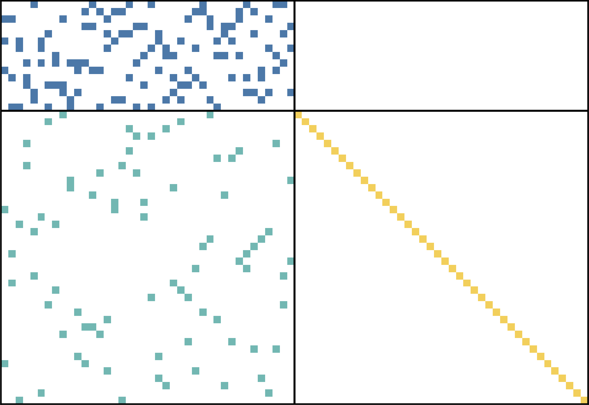
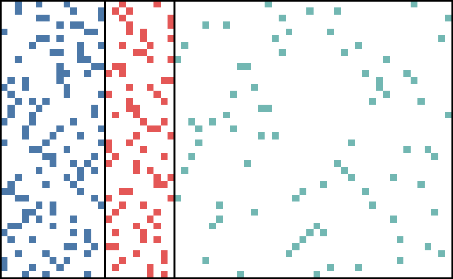
Figure 1: Extended sparse parity-check matrices reproduced from [24]. The upper bitmap is the Z-side matrix \(H'_Z\in\mathbb{F}_2^{55\times80}\), with blocks \(A_Z\), \(B\), and \(I_n\). The lower bitmap is the X-side matrix \(H'_X=[A_X^T\;B^T]=[A_Z^T\;A_\Delta^T\;B^T]\in\mathbb{F}_2^{40\times65}\). The two bitmaps are shown with the same column scale and right alignment, so the rightmost visible-coordinate blocks, both of width 40, have matching horizontal extent. Black lines indicate block boundaries..
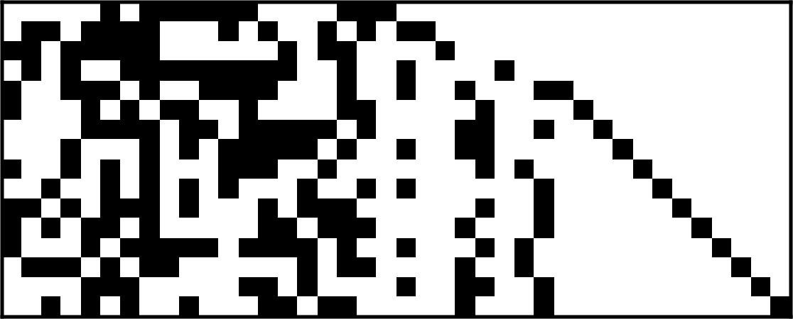
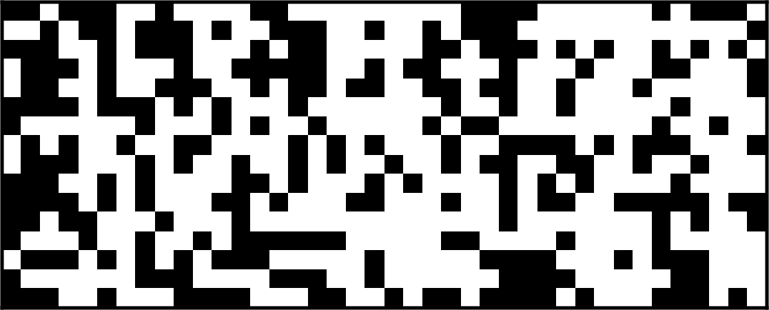
Figure 2: Compressed visible-coordinate parity-check matrices reproduced from [24]. The upper bitmap is the Z-side matrix \(H_Z\in\mathbb{F}_2^{16\times40}\), obtained by projecting a basis of \(\operatorname{Ker}[A_Z^T\;B^T]\) to the visible component. The lower bitmap is the X-side matrix \(H_X=K_XB^T\in\mathbb{F}_2^{15\times40}\), where \(K_X\) is a basis matrix of \(\operatorname{Ker}A_X\). No final reduced row echelon form is applied in the displayed representatives. The two bitmaps are shown with the same horizontal scale because both matrices have 40 visible-coordinate columns..
3 shows one small tail-biting spatially coupled realization of 3 . The example uses \(L=20\), \(w=2\), \(M=8\), \[A_Z^{\mathrm{SC}}\sim(3,8,8,20,2),\qquad A_\Delta^{\mathrm{SC}}\sim(2,8,8,20,2),\qquad B^{\mathrm{SC}}\sim(2,2,8,20,2).\] The two bitmaps display only the sparse extended matrices; the dense visible matrices obtained after puncturing are different objects.
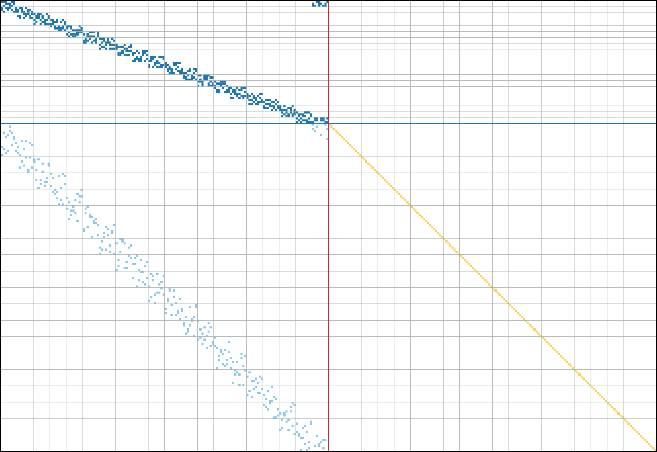
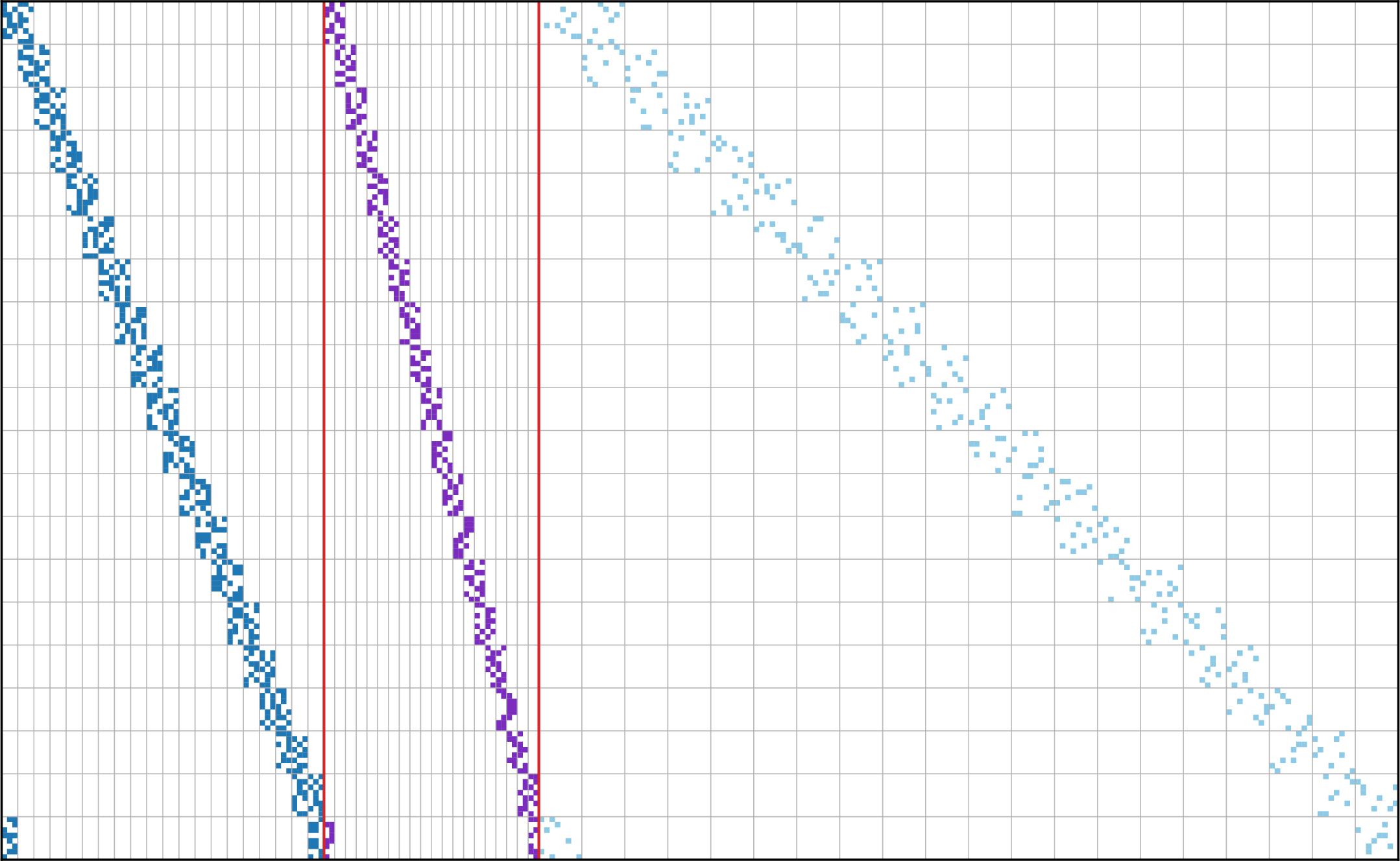
Figure 3: A tail-biting spatially coupled sparse-matrix realization. The upper bitmap is \(H_Z^{\prime\mathrm{SC}}\), with \(A_Z^{\mathrm{SC}}\) in blue, \(B^{\mathrm{SC}}\) in light blue, and \(I_n\) in yellow. The lower bitmap is \(H_X^{\prime\mathrm{SC}}=[(A_X^{\mathrm{SC}})^T\;(B^{\mathrm{SC}})^T]\), with \((A_Z^{\mathrm{SC}})^T\) in blue, \((A_\Delta^{\mathrm{SC}})^T\) in purple, and \((B^{\mathrm{SC}})^T\) in light blue. The two bitmaps are right-aligned and scaled so that the visible, unpunctured \(n\)-coordinate blocks have the same physical width. Thin gray lines mark section boundaries; thick lines mark block boundaries..
For the same realization, 4 displays dense visible-coordinate row bases obtained after puncturing the hidden coordinates. The Z-side matrix is obtained by projecting a basis of \(\operatorname{Ker}[(A_Z^{\mathrm{SC}})^T\;(B^{\mathrm{SC}})^T]\) to the visible block, and the X-side matrix is \(K_X(B^{\mathrm{SC}})^T\), where \(K_X\) is a basis matrix of \(\operatorname{Ker}A_X^{\mathrm{SC}}\). This finite example illustrates that the sparse matrices in 3 represent a generally dense visible-coordinate CSS pair.
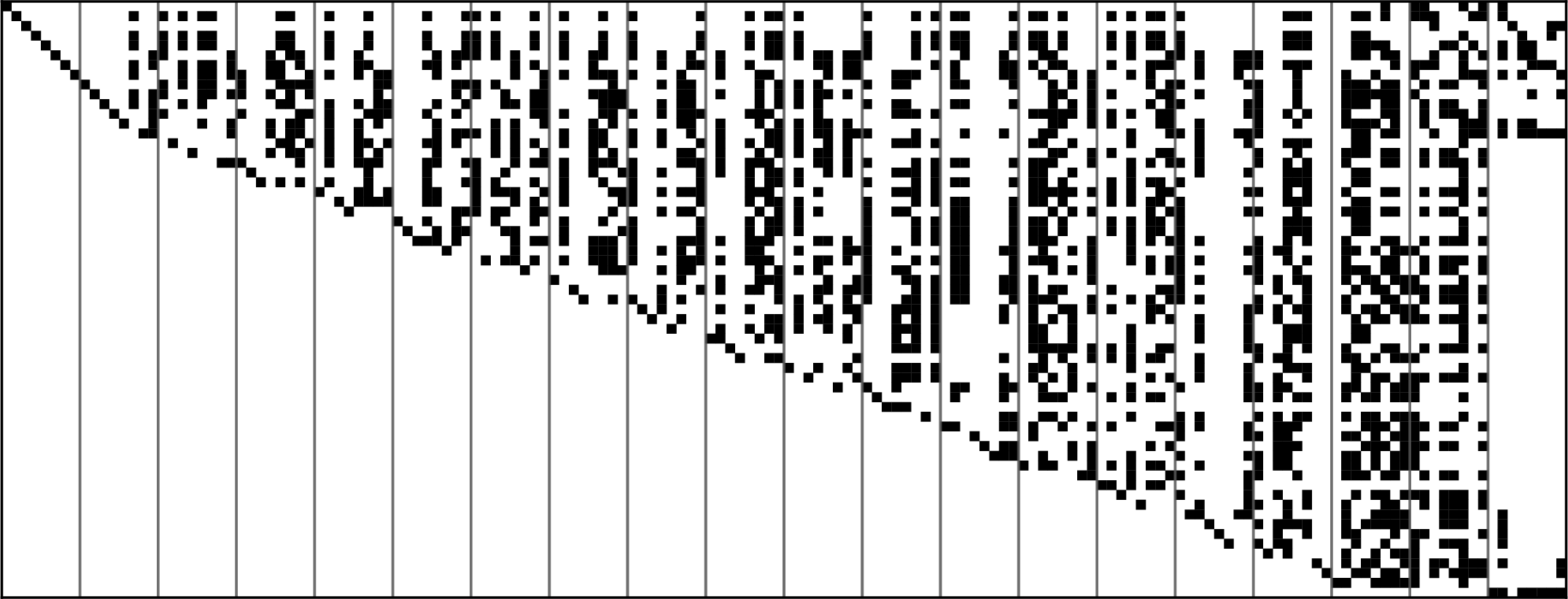
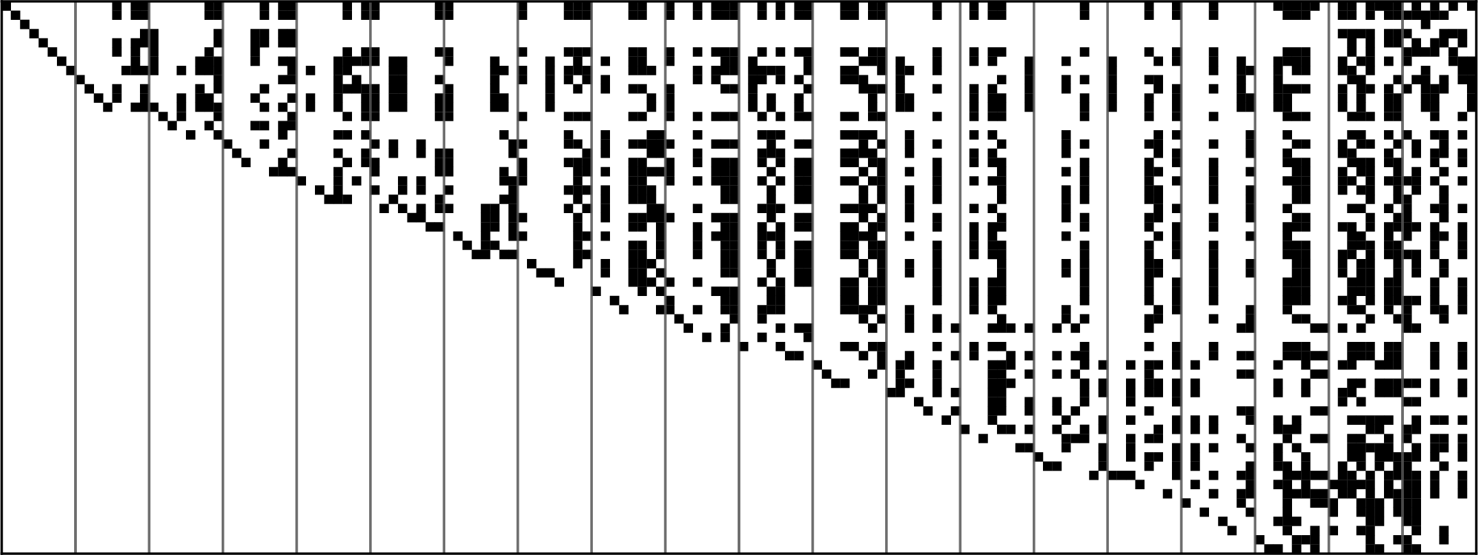
Figure 4: Dense visible-coordinate parity-check row bases corresponding to the tail-biting realization in 3. The upper bitmap is the Z-side matrix \(H_Z\in\mathbb{F}_2^{61\times160}\). The lower bitmap is the X-side matrix \(H_X\in\mathbb{F}_2^{60\times160}\). Both matrices are displayed on the same horizontal scale because they have the same \(n=160\) visible coordinates..
For the DE below, the dense syndrome equations are represented as sparse affine systems after fixed syndrome representatives \(\boldsymbol{t}_Z,\boldsymbol{t}_X\) have been chosen. The Z-side A-check 5 is \[A_Z\boldsymbol{f}_Z=\boldsymbol{0} \label{eq:z-a-check}\tag{5}\] and the Z-side B-check 6 is \[\boldsymbol{e}_X=\boldsymbol{t}_Z+B\boldsymbol{f}_Z. \label{eq:z-b-check}\tag{6}\] This is the sparse representation of the dense syndrome equation involving \(H_Z\boldsymbol{e}_X\). The X-side sparse equations use the stacked matrix and transpose form \[B^T\boldsymbol{e}_Z=\boldsymbol{t}_X+A_X^T\boldsymbol{g}_X. \label{eq:x-side}\tag{7}\] This is the sparse representation of the dense syndrome equation involving \(H_X\boldsymbol{e}_Z\). We call 5 a Z-side A-check, 6 a Z-side B-check, and the constraint in 7 an X-side check. The constant offsets \(\boldsymbol{t}_Z,\boldsymbol{t}_X\) change only the recovered bit values; they do not change whether an erasure message is known or unresolved.
The next proposition computes the design rate of the sparse representation and the hashing-bound channel parameter that is compared with the potential threshold in 7. A quantum erasure leaves two unknown binary Pauli degrees of freedom per erased coordinate. The calculation is the degree-of-freedom form of the erasure hashing/capacity expression in [33].
Proposition 2 (Design rate and hashing-bound parameter). For the finite-degree ensemble of 3 with common check degree \(k\), the constituent design rates are \[R_Z^{\mathrm{des}}=1-\frac{j_Z}{k}, \qquad R_X^{\mathrm{des}}=\frac{j_X}{k},\] and the CSS design rate is \[R_Q^{\mathrm{des}}=\frac{j_X-j_Z}{k}.\] The X/Z equal-rate specialization is the case \(R_Z^{\mathrm{des}}=R_X^{\mathrm{des}}\), equivalently \(j_X=k-j_Z\). It has \[R_Q^{\mathrm{des}}=1-\frac{2j_Z}{k}.\] Equivalently, for a target design rate \(0<\rho<1\), any \(k\) such that \[j_Z=\frac{1-\rho}{2}k,\qquad j_X=\frac{1+\rho}{2}k\] are integers gives an X/Z equal-rate degree triple with \(R_Q^{\mathrm{des}}=\rho\). A purely integral parametrization is \[(j_Z,j_X,k)=(j,j+\lambda,2j+\lambda), \qquad R_Q^{\mathrm{des}}=\frac{\lambda}{2j+\lambda}, \qquad j\geq2,\;\lambda\geq1 .\] For the quantum erasure channel, an erased coordinate leaves two unknown binary Pauli components, and the hashing-bound channel parameter is \[\epsilon_{\mathrm{hash}} =\frac{1-R_Q^{\mathrm{des}}}{2}.\] In the rate-\(1/3\) example \((j_Z,j_X,k)=(4,8,12)\), \[\epsilon_{\mathrm{hash}}=1/3 .\]
Proof. The Z-side visible constituent has \(N\) punctured variables and \(m_Z=(j_Z/k)N\) sparse constraints, giving \(R_Z^{\mathrm{des}}=1-j_Z/k\). The X-side visible constituent has design dimension \(m_Z+m_\Delta=(j_X/k)N\), giving \(R_X^{\mathrm{des}}=j_X/k\). The CSS design rate is \(R_Z^{\mathrm{des}}+R_X^{\mathrm{des}}-1=(j_X-j_Z)/k\). For the quantum erasure channel, each erased coordinate contributes two unresolved binary degrees of freedom, so the conditional degree-of-freedom density is \(2\epsilon\). The hashing-bound condition is \(2\epsilon=1-R_Q^{\mathrm{des}}\). ◻
3 Density Evolution for CSS Erasure Decoding↩︎
The ensembles in 2 are finite random sparse-graph ensembles for each block length. The following standard density-evolution limit gives the asymptotic meaning of the deterministic recursions used in this section.
Theorem 1 (Density-evolution limit for local erasure decoding). Fix the degrees of the sparse CSS ensemble in 3, an erasure probability \(\epsilon\), and a finite number \(\ell\) of BP iterations. As \(N\to\infty\), the depth-\(\ell\) computation neighborhood of a uniformly chosen edge of each message type is tree-like with probability tending to one. Consequently, the expected message-erasure probability after \(\ell\) iterations converges to the value obtained from the corresponding tree recursion [4]. The same local limit applies sectionwise to the tail-biting coupled ensemble of 4 when \(L,w,\ell\) are fixed and \(M\to\infty\). Hence the per-coordinate residual erasure probabilities in the code-length limit are described by the deterministic DE equations stated below.
This theorem justifies replacing a large finite computation neighborhood by a tree recursion for any fixed number of iterations. The rest of the section derives that tree recursion explicitly for the five message types of 3.
The next theorem gives the concrete recursion for the uncoupled finite-degree case with fixed Z-side, X-side, and check degrees. It identifies the deterministic recursion whose fixed points are analyzed in [sec:potential,sec:constituent-positivity]; it is not a finite-length concentration or block-error theorem for the random CSS ensembles.
Let \(a,b\) be the erasure probabilities of messages from a Z-side punctured variable to the Z-side A-check 5 and to the Z-side B-check 6 , respectively. Let \(c\) be the erasure probability of the Z-side visible-component message to the Z-side B-check 6 . Let \(d,e\) be the erasure probabilities of X-side auxiliary-variable and X-side visible-component messages to the X-side check 7 , respectively. The reverse check-to-variable erasure probabilities are \[\begin{align} \hat{a} &=1-(1-a)^{k-1}, \tag{8}\\ \hat{b} &=1-(1-c)(1-b)^{k-1}, \tag{9}\\ \hat{c} &=1-(1-b)^k, \tag{10}\\ \hat{d} &=1-(1-d)^{j_X-1}(1-e)^k, \tag{11}\\ \hat{e} &=1-(1-d)^{j_X}(1-e)^{k-1}. \tag{12} \end{align}\]
Theorem 2 (Hard-erasure density evolution). For CSS erasure decoding over the quantum erasure channel, the abstract local ternary erasure rule is described by \[\begin{align} a^+ &=\hat{a}^{j_Z-1}\hat{b}^k,\\ b^+ &=\hat{a}^{j_Z}\hat{b}^{k-1},\\ c^+ &=\epsilon,\\ d^+ &=\hat{d}^{k-1},\\ e^+ &=\epsilon\,\hat{e}^{k-1}. \end{align} \label{eq:joint-de}\tag{13}\] The residual erasure probabilities of the Z-side and X-side visible components are \[r_Z=\epsilon\,\hat{c},\qquad r_X=\epsilon\,\hat{e}^k. \label{eq:joint-residual}\tag{14}\]
Proof. The check-to-variable updates 8 –12 are the usual erasure-check updates for 5 , 6 , and 7 . A Z-side punctured variable sends an erasure to an A-check iff all other \(j_Z-1\) A-check messages and all \(k\) B-check messages are erased, giving \(a^+\). It sends an erasure to a B-check iff all \(j_Z\) A-check messages and the other \(k-1\) B-check messages are erased, giving \(b^+\). Information about one Pauli component does not determine the other component. Hence the Z-side visible-component message to 6 remains erased exactly when the channel erases the coordinate, giving \(c^+=\epsilon\). The X-side auxiliary-variable update gives \(d^+=\hat{d}^{k-1}\). The X-side visible-component message remains erased when the channel erases the coordinate and the other \(k-1\) X-side check messages are erased, giving \(e^+=\epsilon\hat{e}^{k-1}\). The residual formulas require one additional incoming check message, giving 14 . ◻
The recursion is closed because the hard-erasure rule tracks only whether each message is resolved. Its Z-side and X-side parts will be analyzed by separate potentials, so we now record the two constituent recursions read off from 13 . The Z-side equations use 8 –10 : \[\begin{align} a^+ &=\hat{a}^{j_Z-1}\hat{b}^k,\\ b^+ &=\hat{a}^{j_Z}\hat{b}^{k-1},\\ c^+ &=\epsilon, \end{align} \label{eq:ic-z-de}\tag{15}\] and the Z-side residual is \[r_Z=\epsilon\,\hat{c} . \label{eq:ic-z-residual}\tag{16}\] The X-side equations use 11 –12 : \[\begin{align} d^+ &=\hat{d}^{k-1},\\ e^+ &=\epsilon\,\hat{e}^{k-1}, \end{align} \label{eq:ic-x-de}\tag{17}\] and the X-side residual is \[r_X=\epsilon\,\hat{e}^k . \label{eq:ic-x-residual}\tag{18}\]
4 Vector-Potential Preliminaries↩︎
This section recalls the vector-potential construction for uncoupled density-evolution systems and the corresponding threshold-saturation theorem. The next section specializes these general objects to the Z-side and X-side constituent recursions of this paper.
The term admissible is used below in the standard finite-dimensional sense needed for the coupled-vector potential argument: the recursion is monotone, has enough differentiability for a Taylor expansion, and has scalar primitives from which the potential is built.
Definition 5 (Admissible uncoupled vector DE system). All vectors in this section are column vectors. Let the state space be \([0,1]^d\), ordered coordinatewise, and consider an uncoupled density-evolution system \[\boldsymbol{x}^{+}=\boldsymbol{f}(\boldsymbol{g}(\boldsymbol{x});\epsilon), \qquad 0\leq\epsilon\leq1 .\] This system is called admissible if the following conditions hold.
\(\boldsymbol{f}(\cdot;\epsilon)\) and \(\boldsymbol{g}(\cdot)\) map \([0,1]^d\) into \([0,1]^d\), are twice continuously differentiable on this compact state space, and are coordinatewise nondecreasing. The map \(\boldsymbol{f}(\boldsymbol{y};\epsilon)\) is also nondecreasing in \(\epsilon\).
\(\boldsymbol{g}(\boldsymbol{0})=\boldsymbol{0}\) and \(\boldsymbol{f}(\boldsymbol{g}(\boldsymbol{0});\epsilon)=\boldsymbol{0}\) for every \(\epsilon\). Thus \(\boldsymbol{0}\) is the successful fixed point.
There exist a positive diagonal matrix \(D\) and scalar functions \(F(\boldsymbol{y};\epsilon)\) and \(G(\boldsymbol{x})\) such that \[\nabla F(\boldsymbol{y};\epsilon)=D\boldsymbol{f}(\boldsymbol{y};\epsilon), \qquad \nabla G(\boldsymbol{x})=D\boldsymbol{g}(\boldsymbol{x}).\]
The admissibility conditions are the structural hypotheses needed for the potential method. They ensure that the next definition produces a scalar function whose stationary points coincide with DE fixed points.
Definition 6 (Vector potential for an uncoupled DE system). For an admissible uncoupled vector DE system, with \(D,F,G\) as in 5, the associated vector potential is \[U(\boldsymbol{x};\epsilon) =\boldsymbol{g}(\boldsymbol{x})^T D\boldsymbol{x} -G(\boldsymbol{x})-F(\boldsymbol{g}(\boldsymbol{x});\epsilon). \label{eq:general-vector-potential}\tag{19}\] With the convention \(\inf\emptyset=+\infty\), define \[\mathcal{F}^\star(\epsilon) = \{\boldsymbol{x}\in[0,1]^d\setminus\{\boldsymbol{0}\}: \boldsymbol{x}=\boldsymbol{f}(\boldsymbol{g}(\boldsymbol{x});\epsilon)\}, \qquad \Delta E(\epsilon) = \inf_{\boldsymbol{x}\in\mathcal{F}^\star(\epsilon)} U(\boldsymbol{x};\epsilon). \label{eq:general-energy-gap}\tag{20}\] The potential threshold is \[\epsilon_{\mathrm{pot}} = \sup\{\epsilon_0\in[0,1]: \Delta E(\epsilon)>0 \text{ for every }0\leq\epsilon<\epsilon_0\}. \label{eq:general-potential-threshold}\tag{21}\]
This function is useful because fixed points of the corresponding DE recursion are critical configurations of the potential, and the coupled-vector potential argument measures their cost by \(U\). The energy gap \(\Delta E(\epsilon)\) in 20 is the quantity that controls threshold saturation after spatial coupling.
The next definition fixes the seeded spatially coupled recursion used in the threshold statement. It is written for a general vector DE system, so the same formula applies to any constituent system satisfying 5.
Definition 7 (Seeded spatially coupled DE). Let the state space be \([0,1]^d\), ordered coordinatewise, and let \(\boldsymbol{0}\) be the successful state. Fix a coupling length \(L\), a coupling width \(w\) with \(1\leq w<L\), and a seed interval \(\mathcal{S}\subset\mathbb{Z}/L\mathbb{Z}\). Indices below are taken modulo \(L\). For a profile \(\boldsymbol{X}^{(\ell)}=(\boldsymbol{x}_0^{(\ell)},\ldots,\boldsymbol{x}_{L-1}^{(\ell)})\), define \[\begin{align} \bar{\boldsymbol{x}}_{c}^{(\ell)} &=\frac{1}{w}\sum_{r=0}^{w-1}\boldsymbol{x}_{c-r}^{(\ell)}, \tag{22}\\ \boldsymbol{y}_{c}^{(\ell)} &=\boldsymbol{g}(\bar{\boldsymbol{x}}_{c}^{(\ell)}), \tag{23}\\ \bar{\boldsymbol{y}}_{i}^{(\ell)} &=\frac{1}{w}\sum_{r=0}^{w-1}\boldsymbol{y}_{i+r}^{(\ell)}, \tag{24}\\ \boldsymbol{x}_{i}^{(\ell+1)} &= \begin{cases} \boldsymbol{0}, & i\in\mathcal{S},\\ \boldsymbol{f}(\bar{\boldsymbol{y}}_{i}^{(\ell)};\epsilon), & i\notin\mathcal{S} . \end{cases} \tag{25} \end{align}\] The seeded DE is initialized by \[\boldsymbol{x}_{i}^{(0)} = \begin{cases} \boldsymbol{0}, & i\in\mathcal{S},\\ \boldsymbol{1}, & i\notin\mathcal{S}, \end{cases}\] where \(\boldsymbol{1}\) denotes the largest state in \([0,1]^d\). The recursion is successful in the non-seeded region if \[\lim_{\ell\to\infty}\boldsymbol{x}_{i}^{(\ell)}=\boldsymbol{0} \qquad\text{for every } i\notin\mathcal{S} .\]
The standard threshold-saturation result used below is a general theorem for admissible vector systems. It states that spatial coupling raises the DE threshold to the potential threshold of the uncoupled system.
Theorem 3 (General spatial-coupling threshold saturation, after [18]). Let \[\boldsymbol{x}^{+}=\boldsymbol{f}(\boldsymbol{g}(\boldsymbol{x});\epsilon)\] be an admissible uncoupled vector DE system with vector potential \(U\), successful fixed point \(\boldsymbol{0}\), and potential threshold \(\epsilon_{\mathrm{pot}}\). Form the seeded spatially coupled DE system as in 7. Then, for every \(\epsilon<\epsilon_{\mathrm{pot}}\), there exists a finite coupling width \(w_0(\epsilon)\) such that, for all \(w\geq w_0(\epsilon)\) and sufficiently long coupled chains, the seeded coupled DE converges to the successful fixed point in the non-seeded region. Consequently, the DE threshold of the spatially coupled system is the potential threshold \(\epsilon_{\mathrm{pot}}\) of the uncoupled system.
We use this theorem as a standard result and do not reproduce its shift argument. In the notation of 7, the seed imposes the successful boundary condition \(\boldsymbol{0}\), and the conclusion needed in this paper is that no non-successful coupled fixed point remains outside the seed when \(w\) is sufficiently large and \(\epsilon<\epsilon_{\mathrm{pot}}\). Since the seeded DE iteration is monotone from the largest initial state outside the seed, this absence of non-successful fixed points implies convergence to the successful profile.
5 Constituent Potentials and Fixed Points↩︎
We now instantiate 19 for the two uncoupled DE systems recorded at the end of 3. For the Z-side system 15 , put \[D_Z=\operatorname{diag}(j_Z,k,1),\] and define \[\begin{align} F_Z(\boldsymbol{y}_Z;\epsilon) &=\hat{a}^{j_Z}\hat{b}^k+\epsilon\hat{c}, \tag{26}\\ G_Z(\boldsymbol{x}_Z) &=j_Z\left(a-\frac{1-(1-a)^k}{k}\right) +kb-(1-c)\left(1-(1-b)^k\right). \tag{27} \end{align}\] Then \(\nabla F_Z(\boldsymbol{y}_Z;\epsilon)=D_Z\boldsymbol{f}_Z(\boldsymbol{y}_Z;\epsilon)\) and \(\nabla G_Z(\boldsymbol{x}_Z)=D_Z\boldsymbol{g}_Z(\boldsymbol{x}_Z)\), where \(\boldsymbol{f}_Z\) is the right side of 15 and \(\boldsymbol{g}_Z\) is defined by 8 –10 . The Z-side potential is \[U_Z(\boldsymbol{x}_Z;\epsilon) =\boldsymbol{g}_Z(\boldsymbol{x}_Z)^T D_Z\boldsymbol{x}_Z -G_Z(\boldsymbol{x}_Z)-F_Z(\boldsymbol{g}_Z(\boldsymbol{x}_Z);\epsilon). \label{eq:ic-z-potential}\tag{28}\] For the X-side system 17 , put \[D_X=\operatorname{diag}(j_X,k),\] and define \[\begin{align} F_X(\boldsymbol{y}_X;\epsilon) &=\frac{j_X}{k}\hat{d}^k+\epsilon\hat{e}^k, \tag{29}\\ G_X(\boldsymbol{x}_X) &=j_Xd+ke+(1-d)^{j_X}(1-e)^k-1. \tag{30} \end{align}\] Then \(\nabla F_X(\boldsymbol{y}_X;\epsilon)=D_X\boldsymbol{f}_X(\boldsymbol{y}_X;\epsilon)\) and \(\nabla G_X(\boldsymbol{x}_X)=D_X\boldsymbol{g}_X(\boldsymbol{x}_X)\), where \(\boldsymbol{f}_X\) is the right side of 17 and \(\boldsymbol{g}_X\) is defined by 11 –12 . The X-side potential is \[U_X(\boldsymbol{x}_X;\epsilon) =\boldsymbol{g}_X(\boldsymbol{x}_X)^T D_X\boldsymbol{x}_X -G_X(\boldsymbol{x}_X)-F_X(\boldsymbol{g}_X(\boldsymbol{x}_X);\epsilon). \label{eq:ic-x-potential}\tag{31}\] The stationary points of \(U_Z\) and \(U_X\) are exactly the fixed points of the two constituent recursions.
We now define the fixed-point classes used in the two constituent potential thresholds. The terminology follows the bounded-degree MN/HA potential analysis in [21]; it classifies solutions of the fixed-point equations 15 and 17 , and does not add a channel assumption.
Definition 8 (Successful, trivial, and nontrivial constituent fixed points). Fix \(\epsilon\). Let \(\mathcal{F}_Z(\epsilon)\) be the fixed-point set of 15 . The Z-side successful and trivial fixed-point sets are \[\mathcal{S}_Z(\epsilon) =\{\boldsymbol{x}_Z\in\mathcal{F}_Z(\epsilon):a=b=0\}, \qquad \mathcal{T}_Z(\epsilon) =\{\boldsymbol{x}_Z\in\mathcal{F}_Z(\epsilon):a=b=1\}.\] Here \(c=\epsilon\) at every Z-side fixed point. The Z-side nontrivial fixed-point set is \[\mathcal{N}_Z(\epsilon) =\mathcal{F}_Z(\epsilon)\setminus \bigl(\mathcal{S}_Z(\epsilon)\cup\mathcal{T}_Z(\epsilon)\bigr).\] The Z-side non-successful fixed-point set is \[\mathcal{F}_Z^\star(\epsilon) = \mathcal{F}_Z(\epsilon)\setminus\mathcal{S}_Z(\epsilon) \qquad \left(=\mathcal{T}_Z(\epsilon)\cup\mathcal{N}_Z(\epsilon)\right).\]
Similarly, let \(\mathcal{F}_X(\epsilon)\) be the fixed-point set of 17 . The X-side successful and trivial fixed-point sets are \[\mathcal{S}_X(\epsilon) =\{\boldsymbol{x}_X\in\mathcal{F}_X(\epsilon):d=e=0\}, \qquad \mathcal{T}_X(\epsilon) =\{\boldsymbol{x}_X\in\mathcal{F}_X(\epsilon):d=1,\;e=\epsilon\}.\] The X-side nontrivial fixed-point set is \[\mathcal{N}_X(\epsilon) =\mathcal{F}_X(\epsilon)\setminus \bigl(\mathcal{S}_X(\epsilon)\cup\mathcal{T}_X(\epsilon)\bigr).\] The X-side non-successful fixed-point set is \[\mathcal{F}_X^\star(\epsilon) = \mathcal{F}_X(\epsilon)\setminus\mathcal{S}_X(\epsilon) \qquad \left(=\mathcal{T}_X(\epsilon)\cup\mathcal{N}_X(\epsilon)\right).\]
The successful fixed-point sets represent decoding success and are excluded from the energy-gap minimization. The trivial fixed-point sets are saturated erasure branches whose potentials vanish at the corresponding constituent hashing-bound values. The nontrivial fixed-point sets contain all remaining fixed points.
With the convention \(\inf\emptyset=+\infty\), define \[\Delta E_Z(\epsilon) =\inf_{\boldsymbol{x}_Z\in\mathcal{F}_Z^\star(\epsilon)} U_Z(\boldsymbol{x}_Z;\epsilon), \qquad \epsilon_{\mathrm{pot},Z} =\sup\{\epsilon:\Delta E_Z(\epsilon)>0\}. \label{eq:ic-z-potential-threshold}\tag{32}\] Similarly, define \[\Delta E_X(\epsilon) =\inf_{\boldsymbol{x}_X\in\mathcal{F}_X^\star(\epsilon)} U_X(\boldsymbol{x}_X;\epsilon), \qquad \epsilon_{\mathrm{pot},X} =\sup\{\epsilon:\Delta E_X(\epsilon)>0\}. \label{eq:ic-x-potential-threshold}\tag{33}\] The threshold used for the five-message recursion is \[\epsilon_{\mathrm{pot}} := \min\{\epsilon_{\mathrm{pot},Z}, \epsilon_{\mathrm{pot},X}\}. \label{eq:joint-potential-threshold}\tag{34}\]
6 Nontrivial Constituent Potential Positivity↩︎
This section supplies the nontrivial positivity input used below in [thm:z-constituent-ic-potential,thm:x-constituent-ic-potential]. The trivial fixed points will be handled in those threshold proofs by direct substitution. For the nontrivial fixed points, the proof has four separate parts: first define the two remainder nonnegativity conditions, then explain how each fixed degree reduces to a finite algebraic sign check, then prove the Z-side positivity, and finally prove the X-side positivity.
6.1 Remainder Conditions↩︎
The exact algebraic input is the nonnegativity of two remainders. We define them before stating the corresponding conditions, so that the hypotheses used later are explicit. For the Z side, let \[\hat{a}_Z(a)=1-(1-a)^{k-1}, \qquad \hat{b}_Z(b;\epsilon)=1-(1-\epsilon)(1-b)^{k-1}.\] Define \[\begin{align} \mathcal{R}_Z(a,b;\epsilon) &=(j_Z-1)a\hat{a}_Z(a)+kb\hat{b}_Z(b;\epsilon)-j_Za +\frac{j_Z}{k}\{1-(1-a)^k\}-kb \notag\\ &\quad +\left(1-\frac{j_Z}{k}\right)\{1-(1-b)^k\}. \label{eq:app-z-remainder} \end{align}\tag{35}\] For the X side, let \[\hat{d}_X(d,e)=1-(1-d)^{j_X-1}(1-e)^k, \qquad \hat{e}_X(d,e)=1-(1-d)^{j_X}(1-e)^{k-1}.\] Define \[\begin{align} \mathcal{R}_X(d,e) &=j_Xd\hat{d}_X(d,e)+ke\hat{e}_X(d,e)-j_Xd-ke -(1-d)^{j_X}(1-e)^k+1 \notag\\ &\quad -\frac{j_X}{k}\hat{d}_X(d,e)^k -\left(1-\frac{j_X}{k}\right)\hat{e}_X(d,e)^k . \label{eq:app-x-remainder} \end{align}\tag{36}\] The conditions below state that these explicitly defined remainders are nonnegative on the nontrivial fixed-point branches.
Definition 9 (Algebraic nontrivial positivity conditions). The Z-side condition \(\mathsf P_Z(j_Z,k)\) is the following statement. For every \(0\leq\epsilon<j_Z/k\) and every \(\boldsymbol{x}_Z=(a,b,\epsilon)^T\in\mathcal{N}_Z(\epsilon)\), the quantity \(\mathcal{R}_Z(a,b;\epsilon)\) defined in 35 is nonnegative.
The X-side condition \(\mathsf P_X(j_X,k)\) is the following statement. For every \(0\leq\epsilon<1-j_X/k\) and every \(\boldsymbol{x}_X=(d,e)^T\in\mathcal{N}_X(\epsilon)\), the quantity \(\mathcal{R}_X(d,e)\) defined in 36 is nonnegative.
These conditions are finite-degree algebraic inputs, not additional channel models. The following subsection explains how they can be certified for fixed degrees by eliminating dependent variables from the fixed-point equations.
6.2 Fixed-Degree Certification↩︎
The next proposition explains what remains after the fixed-point equations are used to remove the channel parameter and the message variables that are not independent. For fixed degrees, the conditions \(\mathsf P_Z\) and \(\mathsf P_X\) become finite real-algebraic sign problems.
Proposition 3 (Fixed-degree algebraic certification). For fixed integers \(2\leq j_Z<k\) and \(2\leq j_X<k\), the conditions \(\mathsf P_Z(j_Z,k)\) and \(\mathsf P_X(j_X,k)\) reduce to finite Sturm/resultant sign checks on univariate polynomials. Consequently every fixed X/Z equal-rate family member \((j_Z,j_X,k)=(j,j+\lambda,2j+\lambda)\) has an exact finite certificate problem.
Proof. For the Z side, take a nontrivial fixed point and write \(u=\hat{a}\) and \(v=\hat{b}\). Put \[a_Z(u,v)=u^{j_Z-1}v^k,\qquad b_Z(u,v)=u^{j_Z}v^{k-1}.\] The fixed-point equations give \[a=a_Z(u,v),\qquad b=b_Z(u,v),\] and the check equation \(\hat{a}=1-(1-a)^{k-1}\) gives the algebraic relation \[\Phi_Z(u,v):=u-1+\{1-a_Z(u,v)\}^{k-1}=0 .\] The second check equation recovers the channel value as \[\epsilon=E_Z(u,v):=1-\frac{1-v}{\{1-b_Z(u,v)\}^{k-1}} .\] Since the successful and trivial fixed points are removed, the nontrivial branch has \(0<u,v<1\), and the condition \[0\leq E_Z(u,v)<\frac{j_Z}{k}\] is exactly \(0\leq\epsilon<j_Z/k\). After substituting \(a=a_Z\), \(b=b_Z\), \(\hat{a}=u\), and \(\hat{b}=v\) into 35 , the remainder becomes \[\begin{align} \mathcal{Q}_Z(u,v) &=(j_Z-1)a_Zu+kb_Zv-j_Za_Z +\frac{j_Z}{k}\{1-(1-a_Z)^k\}-kb_Z \notag\\ &\quad +\left(1-\frac{j_Z}{k}\right)\{1-(1-b_Z)^k\}. \label{eq:app-qz-general} \end{align}\tag{37}\] Thus \(\mathsf P_Z(j_Z,k)\) is exactly the nonnegativity of \(\mathcal{Q}_Z\) on this real algebraic branch.
For the X side, write \(u=\hat{d}\) and define \[d_X(u):=u^{k-1},\qquad \Phi_X(u,e):=u-1+\{1-d_X(u)\}^{j_X-1}(1-e)^k=0 .\] Then \(d=d_X(u)\), and the check equation for \(\hat{d}\) gives \(\Phi_X(u,e)=0\). The second check value is \[h_X(u,e):=1-\{1-d_X(u)\}^{j_X}(1-e)^{k-1},\] so the fixed-point equation \(e=\epsilon\hat{e}^{k-1}\) recovers \[\epsilon=E_X(u,e):=\frac{e}{h_X(u,e)^{k-1}} .\] Substituting \(d=d_X\), \(\hat{d}=u\), and \(\hat{e}=h_X\) into 36 gives \[\begin{align} \mathcal{Q}_X(u,e) &=j_Xd_Xu+keh_X-j_Xd_X-ke -\{1-d_X\}^{j_X}(1-e)^k+1 \notag\\ &\quad -\frac{j_X}{k}u^k -\left(1-\frac{j_X}{k}\right)h_X^k . \label{eq:app-qx-general} \end{align}\tag{38}\] Thus \(\mathsf P_X(j_X,k)\) is exactly the nonnegativity of \(\mathcal{Q}_X\) on the real branch with \[0<u<1,\qquad 0\leq e<1,\qquad \Phi_X(u,e)=0,\qquad 0\leq E_X(u,e)<1-\frac{j_X}{k}.\]
It remains to justify that the fixed-degree test is finite and exact. For fixed degrees, \(\Phi_Z,\mathcal{Q}_Z,\Phi_X,\mathcal{Q}_X\) are polynomials with rational coefficients, and the inequalities involving \(E_Z\) and \(E_X\) become polynomial inequalities after clearing denominators that are strictly positive on the displayed branches. The relevant branch endpoints, threshold crossings, vertical tangencies, and possible zeros of \(\mathcal{Q}_Z\) or \(\mathcal{Q}_X\) are roots of univariate resultants. A Sturm sequence isolates these roots and gives the exact sign table on each resulting interval; interval Newton steps then give disjoint rational boxes for the real branch segments. Thus the positivity or failure of positivity is certified by finitely many univariate polynomial sign checks for each fixed degree pair. ◻
Thus the positivity assumptions used below can be checked without rerunning a DE simulation: for each fixed degree pair they reduce to exact polynomial sign tests. The next two subsections show how those algebraic signs enter the potentials.
6.3 Z-Side Positivity↩︎
We now show how the Z-side remainder condition enters the potential. The calculation splits \(U_Z\) into a strictly positive area term and the algebraic remainder \(\mathcal{R}_Z\).
Theorem 4 (Z-side nontrivial positivity). Assume \(2\leq j_Z<k\) and \(\mathsf P_Z(j_Z,k)\). If \(0\leq\epsilon<j_Z/k\), then \[U_Z(\boldsymbol{x}_Z;\epsilon)>0 \qquad \text{for every }\boldsymbol{x}_Z\in\mathcal{N}_Z(\epsilon).\]
Proof. Let \(\boldsymbol{x}_Z=(a,b,c)^T\in\mathcal{N}_Z(\epsilon)\). At every Z-side fixed point, \(c=\epsilon\). Since the fixed point is neither successful nor trivial, \(0<a<1\) and \(0<b<1\). Substituting \(c=\epsilon\) in 15 gives the bounded-degree MN/HA BEC constituent recursion \[a=\hat{a}^{j_Z-1}\hat{b}^k,\qquad b=\hat{a}^{j_Z}\hat{b}^{k-1}, \qquad \hat{a}=1-(1-a)^{k-1},\quad \hat{b}=1-(1-\epsilon)(1-b)^{k-1}.\] Thus \(\mathcal{N}_Z(\epsilon)\) is the nontrivial fixed-point set of that constituent BEC system.
We now expand \(U_Z\). Since \(c=\epsilon\), \(\hat{c}=1-(1-b)^k\), and \(\hat{a}^{j_Z}\hat{b}^k=a\hat{a}\) at a fixed point, 28 becomes \[\begin{align} U_Z(\boldsymbol{x}_Z;\epsilon) &=j_Za\hat{a}+kb\hat{b} -j_Z\left(a-\frac{1-(1-a)^k}{k}\right) -kb+(1-\epsilon)\hat{c}-a\hat{a} \notag\\ &=(j_Z-1)a\hat{a}+kb\hat{b}-j_Za +\frac{j_Z}{k}\{1-(1-a)^k\}-kb+(1-\epsilon)\hat{c} . \label{eq:app-z-expanded} \end{align}\tag{39}\] Separating the area term at the Z-side constituent hashing-bound value gives \[U_Z(\boldsymbol{x}_Z;\epsilon) =\left(\frac{j_Z}{k}-\epsilon\right)\hat{c} +\mathcal{R}_Z(a,b;\epsilon), \label{eq:app-z-area-split}\tag{40}\] where \(\mathcal{R}_Z\) is the remainder defined in 35 . The first term in 40 is strictly positive for \(0\leq\epsilon<j_Z/k\), because \(0<b<1\) implies \(\hat{c}>0\).
The sign of \(\mathcal{R}_Z\) is the only remaining point. The condition \(\mathsf P_Z(j_Z,k)\) states exactly that this remainder is nonnegative on the nontrivial fixed-point set. This is a separate algebraic nonnegativity condition, to be checked on the fixed-point branch for the degrees under consideration. The following convexity identities are elementary inequalities used in such fixed-degree checks; by themselves they do not replace \(\mathsf P_Z(j_Z,k)\). For \(0<t<1\) and \(m\geq2\), \[\frac{1-(1-t)^m}{m}-t(1-t)^{m-1} =\int_0^t (m-1)s(1-s)^{m-2}\,ds>0,\] and \[1-(1-t)^m-mt(1-t)^{m-1} =\int_0^t m(m-1)s(1-s)^{m-2}\,ds>0.\] Thus, under \(\mathsf P_Z(j_Z,k)\), \(\mathcal{R}_Z(a,b;\epsilon)\geq0\) on \(\mathcal{N}_Z(\epsilon)\). Combining this with the strictly positive area term in 40 proves \(U_Z(\boldsymbol{x}_Z;\epsilon)>0\) for \(0\leq\epsilon<j_Z/k\). ◻
6.4 X-Side Positivity↩︎
The X-side proof has the same structure. The fixed-point equation removes the explicit channel factor from \(U_X\), leaving a positive area term and the remainder \(\mathcal{R}_X\).
Theorem 5 (X-side nontrivial positivity). Assume \(2\leq j_X<k\) and \(\mathsf P_X(j_X,k)\). If \(0\leq\epsilon<1-j_X/k\), then \[U_X(\boldsymbol{x}_X;\epsilon)>0 \qquad \text{for every }\boldsymbol{x}_X\in\mathcal{N}_X(\epsilon).\]
Proof. Let \(\boldsymbol{x}_X=(d,e)^T\in\mathcal{N}_X(\epsilon)\). Since the fixed point is neither successful nor trivial, \(0<d<1\). When \(\epsilon>0\), the equation \(e=\epsilon\hat{e}^{k-1}\) gives \(0<e<\epsilon\). When \(\epsilon=0\), any nontrivial fixed point has \(e=0\) and \(0<d<1\). In both cases \(\hat{e}>0\). The fixed-point equations are \[d=\hat{d}^{k-1},\qquad e=\epsilon\hat{e}^{k-1}, \qquad \hat{d}=1-(1-d)^{j_X-1}(1-e)^k,\quad \hat{e}=1-(1-d)^{j_X}(1-e)^{k-1}.\] Expanding 31 gives \[\begin{align} U_X(\boldsymbol{x}_X;\epsilon) &=j_Xd\hat{d}+ke\hat{e}-j_Xd-ke -(1-d)^{j_X}(1-e)^k+1 -\frac{j_X}{k}\hat{d}^k-\epsilon\hat{e}^k . \label{eq:app-x-expanded} \end{align}\tag{41}\] At a fixed point, \(e=\epsilon\hat{e}^{k-1}\), so \(\epsilon\hat{e}^k=e\hat{e}\). Separating the X-side area term gives \[U_X(\boldsymbol{x}_X;\epsilon) =\left(1-\frac{j_X}{k}-\epsilon\right)\hat{e}^k +\mathcal{R}_X(d,e), \label{eq:app-x-area-split}\tag{42}\] where \(\mathcal{R}_X\) is the remainder defined in 36 . The first term in 42 is strictly positive for \(0\leq\epsilon<1-j_X/k\), because a nontrivial fixed point has \(\hat{e}>0\). The condition \(\mathsf P_X(j_X,k)\) states exactly that the remaining term \(\mathcal{R}_X(d,e)\) is nonnegative on \(\mathcal{N}_X(\epsilon)\). Therefore \[U_X(\boldsymbol{x}_X;\epsilon)>0 \qquad (\boldsymbol{x}_X\in\mathcal{N}_X(\epsilon),\;0\leq\epsilon<1-j_X/k).\] ◻
7 Threshold Saturation and X/Z Equal-Rate Degree Families↩︎
The previous section isolated the positivity input for nontrivial fixed points. The next two theorems combine that input with direct computations on the trivial fixed-point branches to identify the two constituent potential thresholds.
Theorem 6 (Z-side potential threshold). Assume \(2\leq j_Z<k\) and the Z-side algebraic positivity condition \(\mathsf P_Z(j_Z,k)\) of 6. Then \[\epsilon_{\mathrm{pot},Z}=\frac{j_Z}{k}.\]
Proof. The successful fixed point has \(a=b=0\) and \(c=\epsilon\); it has \(U_Z=0\) and is excluded from \(\mathcal{F}_Z^\star(\epsilon)\). The Z-side trivial fixed point has \(a=b=1\) and \(c=\epsilon\). Then \(\hat{a}=\hat{b}=\hat{c}=1\), and direct substitution into 28 gives \[\begin{align} U_Z((1,1,\epsilon)^T;\epsilon) &= j_Z+k+\epsilon -\left(j_Z-\frac{j_Z}{k}+k-1+\epsilon\right) -(1+\epsilon) \\ &= \frac{j_Z}{k}-\epsilon . \end{align}\] Thus the trivial Z-side fixed point has positive potential for \(\epsilon<j_Z/k\) and reaches zero at \(\epsilon=j_Z/k\).
For \(\boldsymbol{x}_Z\in\mathcal{N}_Z(\epsilon)\), the fixed point is nontrivial in the classification used for bounded-degree MN/HA potentials [21]. The Z-side nontrivial positivity proved in 4 gives \[U_Z(\boldsymbol{x}_Z;\epsilon)>0 \quad\text{for every } \boldsymbol{x}_Z\in\mathcal{N}_Z(\epsilon) \quad\text{whenever } \epsilon<\frac{j_Z}{k}.\] Together with the previous computation on \(\mathcal{T}_Z(\epsilon)\), this implies \(\Delta E_Z(\epsilon)>0\) for \(\epsilon<j_Z/k\). At \(\epsilon=j_Z/k\), the trivial fixed point has zero potential, and the area/MAP threshold converse for this constituent BEC potential, used in the MN/HA potential analysis of [21], prevents a larger potential threshold. Hence \(\epsilon_{\mathrm{pot},Z}=j_Z/k\). ◻
The X-side threshold is obtained by the same logic, with the complementary degree ratio \(1-j_X/k\) replacing the Z-side ratio \(j_Z/k\).
Theorem 7 (X-side potential threshold). Assume \(2\leq j_X<k\) and the X-side algebraic positivity condition \(\mathsf P_X(j_X,k)\) of 6. Then \[\epsilon_{\mathrm{pot},X}=1-\frac{j_X}{k}.\]
Proof. The successful fixed point \(d=e=0\) has \(U_X=0\) and is excluded. The X-side trivial fixed point has \(d=1\) and \(e=\epsilon\). Then \(\hat{d}=\hat{e}=1\), and \[\begin{align} U_X((1,\epsilon)^T;\epsilon) &= j_X+k\epsilon-(j_X+k\epsilon-1) -\left(\frac{j_X}{k}+\epsilon\right) \\ &= 1-\frac{j_X}{k}-\epsilon . \end{align}\] Thus the trivial X-side fixed point reaches zero at \(\epsilon=1-j_X/k\). For \(\boldsymbol{x}_X\in\mathcal{N}_X(\epsilon)\), the X-side nontrivial positivity proved in 5 gives \[U_X(\boldsymbol{x}_X;\epsilon)>0 \quad\text{for every } \boldsymbol{x}_X\in\mathcal{N}_X(\epsilon) \quad\text{whenever } \epsilon<1-\frac{j_X}{k},\] and the same area/MAP threshold converse used for the bounded-degree MN/HA constituent in [21] excludes a larger X-side potential threshold. Hence \(\epsilon_{\mathrm{pot},X}=1-j_X/k\). ◻
Consequently, \[\epsilon_{\mathrm{pot}} = \min\left\{\frac{j_Z}{k},\,1-\frac{j_X}{k}\right\}. \label{eq:ic-product-potential-value}\tag{43}\]
The five-message recursion separates into the Z-side and X-side constituent recursions. Thus no additional five-message potential is needed. The saturation proof below applies the coupled-vector potential theorem separately to \((\boldsymbol{f}_Z,\boldsymbol{g}_Z,U_Z)\) and \((\boldsymbol{f}_X,\boldsymbol{g}_X,U_X)\). Under the X/Z equal-rate condition \(j_Z+j_X=k\), the threshold in 43 equals the hashing-bound parameter computed in 2.
Remark 1 (Relation to existing potential analyses). The proof route used here follows the established spatial-coupling potential literature. The coupled MN/HA density-evolution equations and numerical BEC threshold evidence appear in [19], and an asymptotic analysis of spatially coupled MN/HA LDPC ensembles appears in [20]. Multi-edge BEC potentials, duality, and bounded-degree MN/HA threshold saturation are treated in [21]; fixed-degree positivity for a bounded-degree MN family is treated in [22]; and the GEC a posteriori probability transfer, area, and SIR potential framework are treated in [23]. The present recursion is decomposed into two BEC constituent systems, and the constituent potential identities, positivity, and spatial-coupling saturation use those arguments separately on the Z and X sides.
The preceding two threshold computations identify the two constituent thresholds. The next theorem packages them into the single threshold relevant to the original five-message CSS recursion and records the simplification under the X/Z equal-rate condition.
Theorem 8 (Constituent potential threshold). Assume \(2\leq j_Z<j_X<k\), \(\mathsf P_Z(j_Z,k)\), and \(\mathsf P_X(j_X,k)\). Then \[\epsilon_{\mathrm{pot}} = \min\left\{\frac{j_Z}{k},\,1-\frac{j_X}{k}\right\}.\] If the additional X/Z equal-rate degree condition \(j_Z+j_X=k\) is imposed, then \[\epsilon_{\mathrm{pot}} =\epsilon_{\mathrm{hash}} =\frac{1-R_Q^{\mathrm{des}}}{2}.\] For \((j_Z,j_X,k)=(4,8,12)\), this value is \(1/3\).
Proof. By the definition 34 and [thm:z-constituent-ic-potential,thm:x-constituent-ic-potential], \[\epsilon_{\mathrm{pot}} = \min\left\{\frac{j_Z}{k},\,1-\frac{j_X}{k}\right\}.\] This proves the general threshold formula. Under \(j_Z+j_X=k\), the two entries in the minimum are both \(j_Z/k\). Since \(R_Q^{\mathrm{des}}=(j_X-j_Z)/k=(k-2j_Z)/k\), \[\frac{j_Z}{k} = \frac{1-R_Q^{\mathrm{des}}}{2} = \epsilon_{\mathrm{hash}} .\] This proves the claimed equality. ◻
The fixed-degree reduction in 3 identifies the finite algebraic sign checks needed to verify the positivity assumptions in 8.
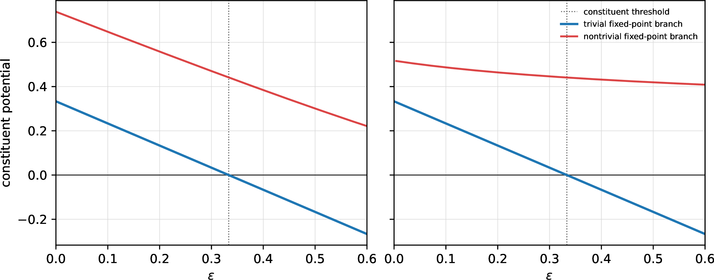
For the X/Z equal-rate example \((j_Z,j_X,k)=(4,8,12)\), 5 plots the constituent potentials on the trivial fixed-point branches and on the numerically found nontrivial fixed points. The trivial branches cross zero at the constituent threshold \(1/3\), while the shown nontrivial fixed-point branches remain positive on the plotted range. This figure is a numerical check of the fixed-point landscape; the exact fixed-degree certificate problem is described in 3.
The next theorem applies this general saturation statement to the two constituent systems. Since the five-message recursion separates into two constituent recursions, saturation of both constituents implies that both residuals in 14 converge to zero.
Theorem 9 (Spatial-coupling saturation). Assume \(2\leq j_Z<j_X<k\), \(\mathsf P_Z(j_Z,k)\), and \(\mathsf P_X(j_X,k)\). Fix \(\epsilon<\epsilon_{\mathrm{pot}}\). For each \(s\in\{Z,X\}\), and for a tail-biting length \(L\) and coupling width \(w\) with \(1\leq w<L\), consider the seeded tail-biting spatially coupled constituent recursion obtained from \((\boldsymbol{f}_s,\boldsymbol{g}_s)\) by the standard modulo-\(L\) window average, \[\bar{\boldsymbol{x}}_{s,c}^{(\ell)} =\frac{1}{w}\sum_{r=0}^{w-1}\boldsymbol{x}_{s,(c-r)\bmod L}^{(\ell)}, \qquad \boldsymbol{y}_{s,c}^{(\ell)}=\boldsymbol{g}_s(\bar{\boldsymbol{x}}_{s,c}^{(\ell)}),\] \[\bar{\boldsymbol{y}}_{s,i}^{(\ell)} =\frac{1}{w}\sum_{r=0}^{w-1}\boldsymbol{y}_{s,(i+r)\bmod L}^{(\ell)}, \qquad \boldsymbol{x}_{s,i}^{(\ell+1)} =\boldsymbol{f}_s(\bar{\boldsymbol{y}}_{s,i}^{(\ell)};\epsilon),\] where \(\boldsymbol{x}_{Z,i}\) is a three-component column vector and \(\boldsymbol{x}_{X,i}\) is a two-component column vector. All components of \(\boldsymbol{x}_{Z,i}\) and \(\boldsymbol{x}_{X,i}\) are fixed to zero on a seed interval \(\mathcal{S}\) of \(w\) consecutive sections. There exists a finite coupling width \(w_0(\epsilon)\) such that, whenever \(w\geq w_0(\epsilon)\) and \(L>w\), no non-successful constituent fixed point remains in the unseeded sections on either side and the residuals converge to zero. Therefore the seeded coupled DE saturates to \(\epsilon_{\mathrm{pot}}\).
Proof. Since \(\epsilon<\epsilon_{\mathrm{pot}}\), the definition 34 gives \(\epsilon<\epsilon_{\mathrm{pot},Z}\) and \(\epsilon<\epsilon_{\mathrm{pot},X}\). The constituent maps \((\boldsymbol{f}_Z,\boldsymbol{g}_Z)\) and \((\boldsymbol{f}_X,\boldsymbol{g}_X)\) are twice continuously differentiable on their compact order intervals, are nondecreasing, and preserve those intervals. Equations 26 –28 and 29 –31 provide the admissible vector potential identities for the Z-side and X-side systems, respectively.
Apply the coupled-vector potential theorem of [18] separately to \((\boldsymbol{f}_Z,\boldsymbol{g}_Z,U_Z)\) and \((\boldsymbol{f}_X,\boldsymbol{g}_X,U_X)\). Equivalently, the standard shift argument applied to each constituent shows that a non-successful coupled fixed point would decrease the corresponding coupled potential by an amount controlled by \(\Delta E_Z(\epsilon)\) or \(\Delta E_X(\epsilon)\), while the second-order window-averaging term is bounded by \(K_s/w\). For sufficiently large \(w\), both constituent systems therefore have only the successful fixed point in the unseeded sections. The five-message DE separates into the two constituent recursions, so the residuals converge to zero. ◻
The X/Z equal-rate degree condition can therefore be used as a rate parameter. The next proposition records the specialization explicitly, separating the rate parameter from the constituent positivity certificates.
Proposition 4 (Rate-parametrized X/Z equal-rate saturation). Let \(0<\rho<1\) and choose \(k\) so that \[j_Z=\frac{1-\rho}{2}k,\qquad j_X=\frac{1+\rho}{2}k\] are integers satisfying \(2\leq j_Z<j_X<k\). Assume \(\mathsf P_Z(j_Z,k)\) and \(\mathsf P_X(j_X,k)\). Then the X/Z equal-rate ensemble has design rate \(R_Q^{\mathrm{des}}=\rho\), and its product potential threshold is \[\epsilon_{\mathrm{pot}} =\epsilon_{\mathrm{hash}} =\frac{1-\rho}{2}.\] Consequently, for every \(\epsilon<(1-\rho)/2\), the seeded tail-biting coupled DE of 9 converges to zero residual for sufficiently large coupling width.
Equivalently, for integers \(j\geq2\) and \(\lambda\geq1\), the one-parameter X/Z equal-rate family \[(j_Z,j_X,k)=(j,j+\lambda,2j+\lambda)\] has \[R_Q^{\mathrm{des}}=\frac{\lambda}{2j+\lambda}, \qquad \epsilon_{\mathrm{pot}} =\epsilon_{\mathrm{hash}} =\frac{j}{2j+\lambda},\] under the corresponding positivity conditions \(\mathsf P_Z(j,2j+\lambda)\) and \(\mathsf P_X(j+\lambda,2j+\lambda)\). The example \((j_Z,j_X,k)=(4,8,12)\) is the case \(j=4,\lambda=4\), hence \(\rho=1/3\).
Proof. The displayed choice satisfies \(j_Z+j_X=k\) and \[\frac{j_X-j_Z}{k} = \frac{(1+\rho)k/2-(1-\rho)k/2}{k} =\rho ,\] so 2 gives \(R_Q^{\mathrm{des}}=\rho\). By 8, the X/Z equal-rate product potential threshold is \[\epsilon_{\mathrm{pot}} = \frac{j_Z}{k} = \frac{1-\rho}{2} = \frac{1-R_Q^{\mathrm{des}}}{2} = \epsilon_{\mathrm{hash}} .\] Then 9 gives convergence of the seeded coupled DE for every \(\epsilon<\epsilon_{\mathrm{pot}}\). Substituting \(\rho=\lambda/(2j+\lambda)\) gives the integral family formulas. For each fixed \((j,\lambda)\), the remaining positivity inputs are exactly the finite algebraic certificate problems described in 6. ◻
We also performed numerical scans of the fixed-degree positivity condition over X/Z equal-rate degree families. First, we exhaustively enumerated all integer triples \((j_Z,j_X,k)=(j,j+\lambda,2j+\lambda)\) with \(2\leq j_Z<j_X<k\leq30\). For each triple, we sampled 17 values of \(\epsilon\) in the interval \([0.025\,\epsilon_{\mathrm{hash}}, 0.975\,\epsilon_{\mathrm{hash}}]\), solved the Z-side and X-side constituent fixed-point equations by continuation from a \(5\times5\) initial-value grid, and checked the constituent potentials at every located nontrivial fixed point. All 182 low-degree X/Z equal-rate triples passed this scan: no negative nontrivial constituent potential was found, and among the 4495 located nontrivial fixed points the smallest potential value was \(0.209101665\).
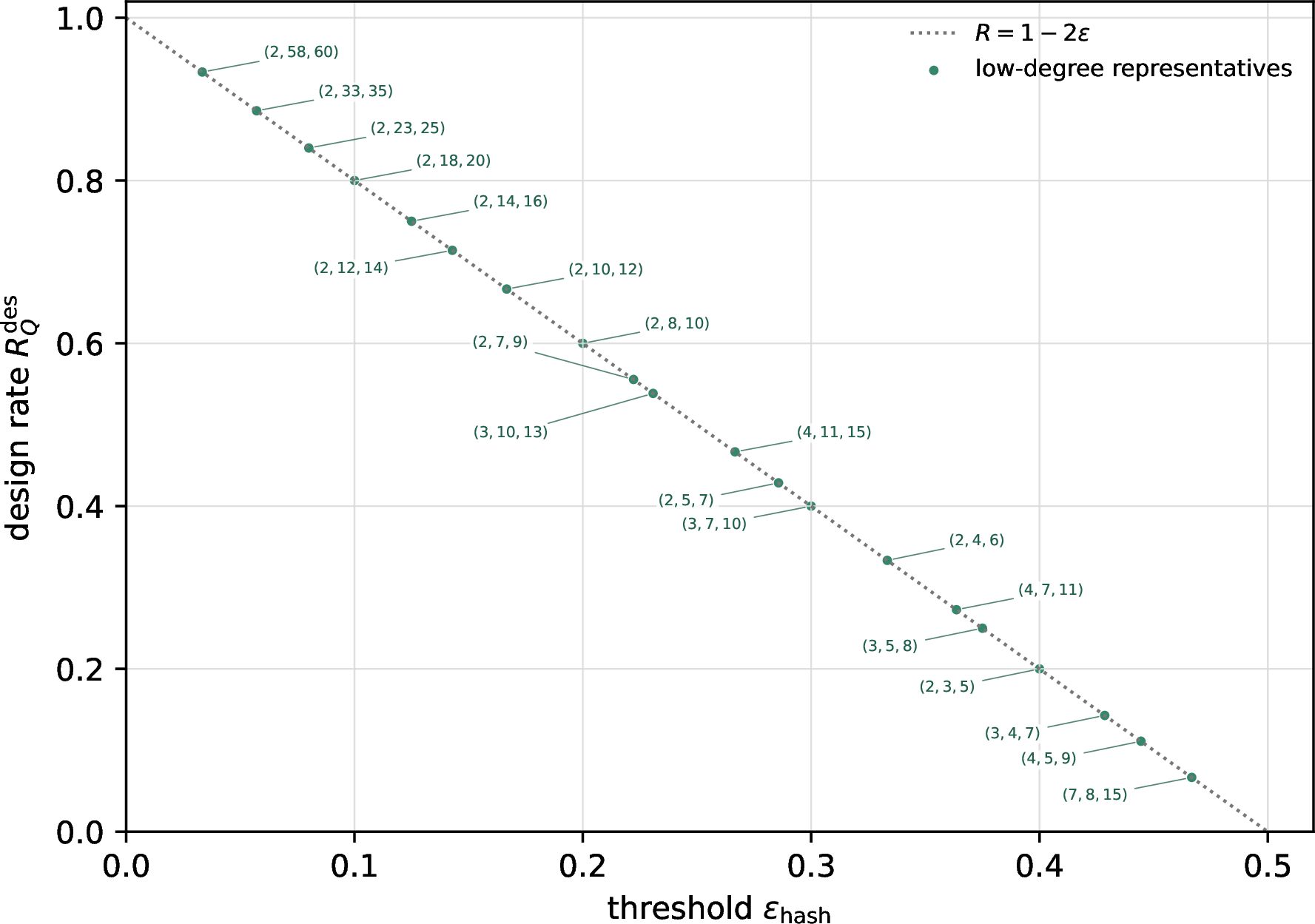
The exhaustive low-degree scan is arithmetically sparse near the endpoint rates, because the constraints \(j_Z\geq2\) and \(k\leq30\) restrict the available rational rates. Therefore 6 also plots about twenty approximately uniform rate representatives. For target rates \(r_i=i/21\), \(i=1,\ldots,20\), we choose an X/Z equal-rate triple \((j_Z,j_X,k)=(j,j+\lambda,2j+\lambda)\) with \(|\lambda/(2j+\lambda)-r_i|\leq0.02\), minimizing \(k\) under this constraint. This gives representatives with \(5\leq k\leq60\). The largest degrees occur only near the high-rate endpoint, where \(j_Z\geq2\) forces \(R_Q^{\mathrm{des}}\leq 1-4/k\). The representative scan did not locate nontrivial fixed points; its role is to display rate coverage with low degrees, while the exhaustive \(k\leq30\) scan above supplies the nontrivial potential samples. Together these scans give numerical evidence for the X/Z equal-rate family across the rate range, while the exact statement remains the finite Sturm/resultant certificate problem in 3.
7.0.0.1 Numerical DE example.
For \((j_Z,j_X,k)=(4,8,12)\), 8 gives \(\epsilon_{\mathrm{pot}}=1/3\). We iterated the seeded tail-biting coupled DE in 9 with \(L=1024\), \(w=16\), a seed interval satisfying \(|\mathcal{S}|=w=16\), and \(\epsilon=0.3325=0.9975\,\epsilon_{\mathrm{pot}}\). The shaded sections in [fig:seeded-ic-z-wave,fig:seeded-ic-x-wave] are the seed sections. The curve at iteration \(0\) is the initial visible-erasure profile \(\epsilon_i\), so it is rectangular. For positive iterations, the plotted quantities are the Z-side and X-side residuals \(r_Z\) and \(r_X\) from 16 and 18 , computed with the coupled check-to-variable averages in 9. Both profiles converged to zero by iteration \(240240\) in this computation.


8 Conclusion and Future Work↩︎
For fixed finite Z-side, X-side, and check degrees, we isolated the hard-erasure recursion associated with the punctured sparse CSS representation, decomposed it into Z-side and X-side constituent systems, and proved seeded spatial-coupling saturation to \(\epsilon_{\mathrm{pot}}=\min\{j_Z/k,\,1-j_X/k\}\). In the X/Z equal-rate specialization \(j_Z+j_X=k\), this threshold equals \(\epsilon_{\mathrm{pot}}=\epsilon_{\mathrm{hash}} =(1-R_Q^{\mathrm{des}})/2\). Equivalently, the rate-parametrized X/Z equal-rate family \((j_Z,j_X,k)=(j,j+\lambda,2j+\lambda)\) has \(R_Q^{\mathrm{des}}=\lambda/(2j+\lambda)\) and \(\epsilon_{\mathrm{pot}}=j/(2j+\lambda) =(1-R_Q^{\mathrm{des}})/2\), subject to the same constituent positivity certificates.
The scope of this theorem is deliberately deterministic and asymptotic at the DE level. The seed in 9 is an ideal boundary condition: on a seed interval \(\mathcal{S}\), all message-erasure components \(a,b,c,d,e\) are fixed to zero, equivalently the local channel parameter is replaced by \(\epsilon_i=0\) on those sections. A finite CSS realization of this complete DE seed is not provided here. Such a realization would need operations on the visible CSS code, or on an enlarged CSS code with additional known degrees of freedom, that make all sparse-representation messages in the seed sections known while preserving CSS commutation and the syndrome interface in 4 . Shortening or puncturing only selected visible coordinates would define a different finite ensemble whose DE must be analyzed separately.
The result should also be read as a bitwise DE threshold statement, not as a finite-length block-error theorem. The residuals \(r_Z\) and \(r_X\) are per-coordinate residual erasure probabilities. For a finite code of visible length \(n\), block success requires the whole residual ambiguity to be CSS-stabilizer equivalent to zero with probability tending to one. This calls for finite-length ingredients beyond the present paper: a concentration or replacement argument connecting the deterministic recursion to the intended random finite ensemble, a scaling choice for the gap to threshold, chain length, coupling width, seed, and number of iterations, and a final CSS logical-success criterion. Classical iterative-decoding analyses compare the weak-sense, bit-error limit with the strong-sense, block-error limit [34]; adapting that bridge to the present CSS erasure setting is a separate finite-length problem. Another useful next step is to develop Sturm/interval certificates for \(\mathsf P_Z\) and \(\mathsf P_X\) into an exact certification method for broader X/Z equal-rate degree families.