Signed-Permutation Coordinate Transport for RMSNorm Transformers
June 30, 2026
Abstract
Modern LLM workflows increasingly move coordinate-indexed objects across checkpoints: steering vectors, sparse autoencoders, top-\(k\) neuron sets, attribution lists, and merge alignments. This is only well posed after fixing the model’s residual-stream gauge. We show that the native discrete gauge is architecture-dependent: LayerNorm residual charts have permutation gauge \(S_d\), up to a global sign flip, while RMSNorm residual charts with generic per-channel gain have signed-permutation gauge \(B_d=S_d\ltimes\{\pm1\}^d\). Thus permutation-only alignment is symmetry-incomplete for RMSNorm models. We introduce sign-marginalized Hungarian matching and prove a sharp population failure mode: with decorrelated source coordinates, raw signed-correlation matching has a structural permutation-accuracy ceiling equal to the fraction of positive signs in the true gauge up to \(O(d2^{-d})\), whereas sign-marginalized matching removes this obstruction. We then make coordinate-preserving transport, rather than function-level merging, the primary object: composing saved-checkpoint local \(B_d\) gauges along same-base fine-tuning trajectories recovers 91.1% of cross-run coordinates at 1500 steps versus 60.3% for endpoint matching, and the gain is not explained by merely routing through the base. The recovered gauge transfers tools that permutation-only alignment breaks: TinyLlama SAE reconstruction has NMSE 0.004 under \(B_d\) recovery versus 1.08 under \(S_d\); Qwen sentiment steering preserves 95.8% of its effect versus 17.2%; refusal steering reverses sign under \(S_d\). Coordinate-preserving merge tests show the same mechanism. The same covariance governs stateful training: signed transport of AdamW state preserves the resumed trajectory, while permutation-only state transport starts from a functionally identical checkpoint but follows a different trajectory. Finally, we give gauge-sweep audits for index-level interpretability claims: coordinate names are reproducible only relative to an explicit gauge.
1 Introduction↩︎
The question “which neuron is this?” is ill-posed without a gauge specification. If a residual coordinate of a transformer is relabeled, the input-output function is unchanged but every index-level object attached to that coordinate moves with the relabeling. This is not merely philosophical: modern workflows publish coordinate-indexed artifacts–ranked neuron or attribution sets, knowledge-neuron edits, SAE dictionaries, steering directions, LoRA updates, and merge alignments. A coordinate-indexed claim should therefore pass a simple audit: exact gauges should preserve behavior, move raw coordinate names, and restore agreement after mapping back.
Standard alignment tools such as Git Re-Basin and weight matching search over permutations [Ainsworth et al., 2023, Entezari et al., 2022]. That is correct for LayerNorm residual streams, but widely used open-weight LLMs such as Llama 2 and Qwen2.5 use RMSNorm [Touvron et al., 2023, Yang et al., 2024a, Zhang and Sennrich, 2019]. RMSNorm lacks mean-centering. Its residual stream therefore admits not only permutations but independent sign flips of every coordinate. The relevant discrete group is the hyperoctahedral group \(B_d\) of order \(2^d d!\), not \(S_d\) of order \(d!\). In a 4096-dimensional residual stream, the omitted sign component fixes only one of \(2^{4096}\) gauge cosets and forgoes 4096 binary degrees of freedom; Corollary 1 shows that mis-applying it to a learned weight update introduces squared error of magnitude \(2\left\lVert \Delta W \right\rVert_F^2\) in expectation, the same order as the update’s own energy. Many analyses are already gauge-invariant; our target is workflows that explicitly move or publish coordinate-indexed artifacts.
This paper is about the consequences of using the right group. We first prove that LayerNorm has \(S_d\), up to a global sign flip, while RMSNorm has full signed-permutation gauge \(B_d\) for generic gain \(\gamma\), and that \(B_d\) is the maximal coordinate-preserving subgroup of \(O(d)\) in the native \(\gamma\)-explicit parameterization. Broader orthogonal freedom returns only after absorbing \(\gamma\) into adjacent weights; this is useful for compression or dense fusion, but it changes the coordinate system and does not preserve sparse coordinate identity.
We then recover the gauge from activations. The natural algorithm is the activation-matching linear assignment used by earlier neuron-alignment and Git Re-Basin work [Li et al., 2016, Tatro et al., 2020, Ainsworth et al., 2023], solved by Hungarian-style assignment methods [Kuhn, 1955], except that the cost must marginalize over sign: match columns by \(|\left\langle h_i,h'_j \right\rangle|\), then recover the sign from the matched correlation. The absolute value is required by the \(B_d\) symmetry: under a negative gauge sign, the correct coordinate is maximally anti-correlated. We prove this ceiling in the decorrelated-coordinate population case: when half the true signs are negative, the correct entries for those coordinates are the most negative entries in their rows, so signed-correlation maximization avoids them even with unlimited probes. Recorded-gauge LLM activations show the same obstruction: signed-cost recovery stays near 50%, while sign-marginalized recovery reaches 100%.
The constructive payoff is transport when an atlas exists. Instead of matching only two endpoints, we compose saved-checkpoint local \(B_d\) gauges along a training trajectory. On a gauge-instrumented Qwen2.5-1.5B fine-tuning benchmark (1500 steps, with a randomly sampled \(B_d\) gauge applied at step 0 and its induced correspondence recorded as ground truth), endpoint matching recovers 60.3% of coordinates while transport-via-base recovers 91.1%; endpoint-via-base recovers only 11.4%, so the improvement is not a base-reference artifact but comes from many small, high-margin local gauges. The result is \(B_d\)-specific: \(S_d\)-only transport drops signs and reverses transferred tools; continuous-rotation atlases preserve function but lose coordinate identity (Theorem 2); only \(B_d\) preserves both, so steering vectors and adapters transfer cleanly under \(B_d\) recovery.
The same sign failure mode appears in coordinate-preserving merge tests. In a Llama-2-7B gauge-scramble merge, signed alignment eliminates the peak-above-chord barrier (\(6.14\to0.00\)), while exact permutation-only alignment is actively harmful. In independently trained 10M-parameter RMSNorm transformers, sign mismatch appears between seeds without an external basis change, and signed alignment improves the barrier from 0.66 to 0.42 over permutation-only. These merge results are scoped to the coordinate-preserving regime: when coordinate identity is the object, RMSNorm alignment must include signs. The same gauge covariance governs AdamW optimizer state: signed transport preserves the resumed training trajectory, while permutation-only state diverges despite starting from a functionally identical checkpoint.
Finally, we use gauge sweeps as a falsifiable negative control for coordinate-indexed interpretability. Coordinates are not always the right units; directions, subspaces, CKA, and behavior-level interventions are often better and already gauge-invariant [Raghu et al., 2017, Morcos et al., 2018, Kornblith et al., 2019]. But the field still produces coordinate-indexed artifacts–knowledge neurons, top-\(k\) steering coordinates, SAE feature dictionaries, sparse ablation sets–and these are reproducible only relative to a gauge. Cross-run reproducibility for such claims requires a gauge anchor (e.g., a same-base atlas), \(B_d\)-correct READ/WRITE rules for any artifact crossing parameterizations, and the audit as a negative control: under an exact random gauge, raw indices should move, mapped indices should agree, and behavior should remain fixed.
2 Native residual-stream gauge↩︎
We use row-vector notation. A residual activation matrix \(H\in\mathbb{R}^{n\times d}\) is gauged by right multiplication \(H\mapsto HG\). A signed permutation \(G\in B_d\) has exactly one nonzero entry, \(\pm1\), in each row and column. A permutation is the special case with all signs \(+1\). We use “gauge” in the reparameterization sense: a choice of coordinates within a function-preserving symmetry orbit. In this paper the relevant group is the global discrete signed-permutation action \(B_d\) on residual coordinates.
Theorem 1 (Maximal native discrete gauge). Consider a transformer with residual dimension \(d\), tokenwise LayerNorm or RMSNorm, standard affine projections \(Y=XW^\top+b\), and attention/MLP sublayers that interact with residual coordinates only through linear maps, elementwise nonlinearities, and the normalization. Then the following groups act by function-preserving residual-coordinate relabelings: \[\mathcal{G}= \begin{cases} \{\pm P:P\in S_d\}\cong S_d\times C_2, & \text{LayerNorm},\\ B_d, & \text{RMSNorm with generic per-channel gain }\gamma. \end{cases}\] For LayerNorm, the \(C_2\) factor is one global sign flip with \(\beta\mapsto-\beta\), so the per-index content is still \(S_d\). Moreover, for generic RMSNorm \(\gamma\), \(B_d\) is the maximal subgroup of \(O(d)\) that preserves native coordinate identity without absorbing \(\gamma\) into adjacent weights. Repeated \(\gamma\) values can add rotations inside common equal-\(\gamma\) subspaces across RMSNorms sharing the residual chart; if any relevant gain vector is generic, the native orthogonal gauge reduces to \(B_d\).
2.0.0.1 Proof sketch.
Linear maps admit any orthogonal residual gauge under READ/WRITE weight transforms. A READ map uses \(W^G=WG\), giving \(HG(W^G)^\top=HW^\top\); a WRITE map uses \(W^G=G^\top W\), \(b^G=bG\), giving \((XW^\top+b)G\). \(Q,K,V\) projections are invariant; only the output projection writes the gauged contribution. Normalization restricts \(G\). RMSNorm is norm-invariant, but its diagonal gain requires \(G^\top\operatorname{diag}(\gamma)G\) to remain diagonal; for generic \(\gamma\), the orthogonal solutions are exactly signed permutations. LayerNorm is permutation-invariant but excludes independent coordinate signs; the remaining signed elements are \(-P\), with \(\beta\mapsto-\beta P\) (Lemma 3). Full module rules and induction over blocks are in Appendices 9 and 13.
The native-vs.-absorbed distinction is the main boundary with recent orthogonal methods. SliceGPT and QuaRot exploit the identity \(\operatorname{RMSNorm}(XQ)Q^\top=\operatorname{RMSNorm}(X)\) after moving gains into neighboring matrices [Ashkboos et al., 2024a,b]; generalized linear mode connectivity and rotation-based fusion use related \(O(d)\) structure [Theus et al., 2025, Zhang et al., 2025]. These methods are complementary. They are appropriate when a dense rotated basis is acceptable. Transporting a top-\(k\) coordinate set, an SAE dictionary attached to residual coordinates, an AdamW diagonal state, or an index-level claim requires the native coordinate-preserving subgroup, which is \(B_d\) (Proposition 8 and Remark 7).
Theorem 2 (Discrete content of an orthogonal map). For any \(Q\in O(d)\), define \[P^\star = \operatorname*{arg\,min}_{P\in B_d}\left\lVert Q-P \right\rVert_F .\] Generically (outside a Lebesgue-null set of \(Q\) where Hungarian ties or matched zeros occur), \(P^\star\) is obtained by Hungarian assignment on \(|Q|\): choose \[\sigma^\star = \operatorname*{arg\,max}_{\sigma\in S_d}\sum_j |Q_{\sigma(j),j}|,\] then set the sign of column \(j\) to \(\operatorname{sign}(Q_{\sigma^\star(j),j})\). The residual \(R=Q(P^\star)^{-1}\in O(d)\) captures continuous drift, and \(\rho(Q)=d^{-1}\operatorname{tr}(Q^\top P^\star)\) equals one iff \(Q\in B_d\).
Theorem 2 separates the two alignment objects. The \(B_d\) component is a discrete scaffold that preserves coordinate identity; the residual \(R\) is a dense basis change. In limited-data settings this matters: estimating an arbitrary dense \(R\) requires paired activation information at scale, while the discrete component of a known orthogonal map is recovered from \(|Q|\) alone. Proof is in Appendix 12.
Proposition 3 (Gauge-covariance of learned weight updates). Let \(\theta\) be a transformer parameterization satisfying the assumptions of Theorem 1, and let \(G\in\mathcal{G}\) be an admissible discrete gauge. Write \(T_G\) for the modulewise READ/WRITE/RMSNorm transform of Theorem 1 acting on weights. Then \(T_G\) is linear: for any weight delta \(\Delta\theta\) on the same parameter set, however produced, \[T_G(\theta+\Delta\theta)=T_G(\theta)+T_G^{\mathrm{lin}}(\Delta\theta),\] where \(T_G^{\mathrm{lin}}\) applies the same modulewise READ/WRITE rules to \(\Delta\theta\) as a free linear map. In particular, for a low-rank LoRA factor \(\Delta W=BA\) on a residual-stream projection, \[\text{READ: } A^G=AG,\;B^G=B;\qquad \text{WRITE: } A^G=A,\;B^G=G^\top B.\]
Corollary 1 (Sign-omission destroys learned updates). For an update \(\Delta W\) on a coordinate-indexed module under RMSNorm gauge \(G=PS\) with permutation \(P\) and signs \(S=\operatorname{diag}(s)\), \(s_j\in\{\pm1\}\), the squared Frobenius update error of \(S_d\)-only transport (correct permutation, signs forced to \(+1\)) is \[\left\lVert \Delta WPS-\Delta WP \right\rVert_F^2 =4\sum_{j:s_j=-1}\left\lVert \Delta W_{:,P^{-1}(j)} \right\rVert_2^2, \qquad \mathbb{E}_S[\cdot]=2\left\lVert \Delta W \right\rVert_F^2.\] For random signs, the expected error equals twice the update’s own energy.
2.0.0.2 Empirical confirmation.
In our Qwen2.5-1.5B SST-2 LoRA experiment (Table 5), \(S_d\)-perm-only transport gives accuracy 0.523 versus the unadapted base 0.525–i.e., a \(-0.5\%\) adapter-gain preservation, consistent with the sign-omission collapse predicted by Corollary 1. The signed transport recovers 0.944, matching the source adapter (0.945) and the upper-bound reference (0.944).
Lemma 1 (Artifact orientation). Let \(G=P\operatorname{diag}(s)\in B_d\) with \(s\in\{\pm1\}^d\). For any residual-aligned vector artifact \(v\in\mathbb{R}^d\)–a steering vector, cached activation, linear-probe direction, SAE encoder row, or LoRA READ-side row–the correct \(B_d\) transport is \(vG\), while permutation-only (\(S_d\)) transport is \(vP\) (WRITE-side matrices and SAE decoder columns transform via \(G^\top\); see Table 1). These satisfy \[\left\lVert vG-vP \right\rVert_2^2 =4\sum_{j:s_j=-1}(vP)_j^2,\qquad \cos\angle(vG,vP)= \frac{\sum_j s_j(vP)_j^2}{\sum_j(vP)_j^2}.\] For balanced signs and a \(vP\) not concentrated on a few coordinates, the cosine is near zero: \(S_d\) preserves the support of \(v\) but loses its orientation.
Lemma 1 is the vector specialization of Corollary 1 and unifies all \(B_d\)-specific tool-transfer outcomes in this paper: each artifact in Table 1 has a coordinate-indexed orientation that \(S_d\) alignment cannot represent, and each gauge-covariance row in Table 5 is one instance of the same orientation law.
| Artifact | Correct \(\Bd\) transport | What \(\Sd\) misses |
|---|---|---|
| Steering vector \(v\) | \(v\mapsto vG\) | sign orientation |
| Cached residual/patch \(h\) | \(h\mapsto hG\) | cached-state orientation |
| Linear probe direction \(w\) | \(w\mapsto wG\) | decision-boundary orientation |
| SAE encoder \(W_{\rm enc}\) | \(W_{\rm enc}\mapsto W_{\rm enc}G\) | feature-read orientation |
| SAE decoder \(W_{\rm dec}\) | \(W_{\rm dec}\mapsto G^\top W_{\rm dec}\) | reconstruction orientation |
| LoRA READ \(\Delta W=BA\) | \(A\mapsto AG,\;B\mapsto B\) | input-basis signs |
| LoRA WRITE \(\Delta W=BA\) | \(A\mapsto A,\;B\mapsto G^\top B\) | output-basis signs |
| AdamW/SGDm first moment \(m_W\) | \(m_W\) transforms with \(W\) (per role) | first-moment orientation |
| AdamW second moment \(v_W\) | \(v_W\mapsto T_{|G|}(v_W)\) (perm only; signs square out) | none—\(v\) is sign-blind by construction |
2.0.0.3 Gauge-invariance validation.
We verify Theorem 1 by applying random gauges and measuring max logit deviation on held-out prompts or images. LayerNorm models pass permutation gauges and fail independent sign-flip gauges; RMSNorm/T5LayerNorm models pass full signed gauges. Biases must transform as WRITE vectors. Table 2 reports cross-architecture checks; Figure 1 in the appendix gives the corresponding off-group validation cases.
The audit does not invalidate the behavior-level conclusions of these analyses. It separates invariant claims from coordinate claims: the refusal direction still changes refusal behavior, and the steering vectors still steer, but the coordinate names attached to those objects are not invariant artifacts until a gauge is specified.
| Model | Norm | Gauge | Max logit error |
|---|---|---|---|
| Qwen2.5-7B | RMSNorm | \(\Bd\) | \(1.1\times10^{-4}\) |
| Llama-3.1-8B | RMSNorm | \(\Bd\) | \(3.0\times10^{-5}\) |
| TinyLlama-1.1B | RMSNorm | \(\Bd\) | \(8.6\times10^{-5}\) |
| BERT-base | LayerNorm | \(\Sd\) | \(2.3\times10^{-5}\) |
| T5-small | T5LayerNorm | \(\Bd\) | \(7.6\times10^{-5}\) |
| ViT-B/16 | LayerNorm | \(\Sd\) | \(4.3\times10^{-6}\) |
3 Sign-marginalized gauge recovery↩︎
Given paired probe activations \(H_s,H_t\in\mathbb{R}^{n\times d}\), we want a recovery action matrix \(G\in B_d\) such that \(H_tG\approx H_s\). Center
columns and set \(C=H_s^\top H_t\). For a correspondence \(\pi\) and signs \(s_i\), minimizing \[\sum_i \left\lVert
H_s[:,i]-s_iH_t[:,\pi(i)] \right\rVert_2^2\] is equivalent to maximizing \(\sum_i s_i C_{i,\pi(i)}\). For fixed \(\pi\), the optimal sign is \(s_i=\operatorname{sign}(C_{i,\pi(i)})\), so the problem reduces to \[\pi^\star=\operatorname*{arg\,max}_{\pi\in S_d}\sum_i |C_{i,\pi(i)}|,
\qquad
s_i^\star=\operatorname{sign}(C_{i,\pi^\star(i)}).\] This is a standard linear assignment on \(-|C|\). We solve it with SciPy’s linear_sum_assignment routine, a modified Jonker-Volgenant implementation;
the assignment problem and shortest-augmenting-path algorithms are classical [Kuhn, 1955, Jonker and Volgenant, 1987, Crouse, 2016, Virtanen et al., 2020].
3.0.0.1 Permutation/sign convention.
Write \(P_\pi\) for the row-action permutation with \((P_\pi)_{i,\pi(i)}=1\), so \((hP_\pi)_{\pi(i)}=h_i\). Matching returns source-indexed signs \(s_i=\operatorname{sign}(C_{i,\pi(i)})\) and \(S_s=\operatorname{diag}(s_i)\). The forward gauge is \(G_{\rm fwd}=S_sP_\pi\), so \(H_t\approx H_sG_{\rm fwd}\); the recovery action is \(G_{\rm rec}=P_\pi^\top S_s=G_{\rm fwd}^{-1}\), so \(H_tG_{\rm rec}\approx H_s\). Equivalently, with target-indexed \(S_t=P_\pi^\top S_sP_\pi\), \(G_{\rm fwd}=P_\pi S_t\); later formulas writing \(G=P\operatorname{diag}(s)\) use target-indexed signs. This section reports recovery matrices; Section 4 switches to forward-direction subscripts.
Theorem 4 (Structural ceiling in the decorrelated-coordinate case). Suppose two activation matrices are related by a true signed permutation \((\pi^\star,s^\star)\), and source coordinates are uncorrelated with positive variances. Let \[\hat{\pi}_{\rm signed}=\operatorname*{arg\,max}_\pi\sum_i C_{i,\pi(i)},\qquad \hat{\pi}_{\rm abs}=\operatorname*{arg\,max}_\pi\sum_i |C_{i,\pi(i)}|.\] As \(N\to\infty\), \(\hat{\pi}_{\rm signed}\)’s accuracy equals the positive-sign fraction except in the one-negative-sign case; under iid signs its expectation is \(1/2+O(d2^{-d})\). The sign-marginalized estimator \(\hat{\pi}_{\rm abs}\) converges to the true permutation under the assignment-margin condition of Lemma 8.
The theorem explains why permutation-only RMSNorm alignment can fail even with unlimited probes. If the true sign is negative, the correct entry is the row’s most negative correlation; signed-correlation matching is designed to avoid it. Correlated residual coordinates can change the exact ceiling, but not the sign-marginalization requirement: under a negative gauge sign, the true coordinate is anti-correlated with its source coordinate, so signed-correlation matching is optimizing the wrong objective.
In recovery experiments where a recorded \(B_d\) basis change provides the target correspondence, naive Hungarian on signed cost recovers only 49.4%–49.9% of the permutation and about 50.1% of signs on 7B/8B RMSNorm models, matching the predicted sign obstruction; sign-marginalized matching recovers 100% on the same rows (Table 15). The same recovery succeeds with as few as 22 probe tokens on TinyLlama (Appendix 15.2). Gradient-times-activation attribution is also restored: signs cancel in \((hG)\odot((\nabla_h L)G)=(h\odot\nabla_h L)P\), so the recovered permutation maps top-\(k\) attribution indices back exactly.
3.0.0.2 Probe-budget regimes.
The experiments use three regimes, summarized in Table 3: settings with a recorded gauge correspondence are probe-robust; same-base fine-tuning trajectory transport works with small local probes because consecutive checkpoints have high assignment margins; natural alignment between independently trained or differently trained models is probe-hungry and is reported as stability against a large-probe reference rather than as exact accuracy.
| Result family | Probe budget | Setting |
|---|---|---|
| Gauge-instrumented recovery | 22–500 tokens | known reference basis |
| Gauge-scramble merge | \(\sim\)500 tokens | basis change + 50-step fine-tune |
| Transport trajectory recovery | \(\sim\)500 tokens/local match | same-base fine-tunes |
| Qwen \(\Bd\) vs. \(\Sd\) steering | \(\sim\)500 tokens | same-base fine-tunes |
| TinyLlama SAE/steering transfer | 11,134 tokens | basis-change tool transfer |
| Independent-seed RMSNorm merge | \(\sim\)500 tokens | same data, different seeds |
| Natural cross-model stability | \(\sim\)36K tokens (saturated) | no reference basis |
4 Parallel transport and tool transfer↩︎
Endpoint matching estimates one gauge; transport composes many local ones. For a trajectory \(t_0,t_1,\ldots,t_T\), estimate \(G_{t_k\to t_{k+1}}\) by sign-marginalized matching with \(H_{t_k}G_{t_k\to t_{k+1}}\approx H_{t_{k+1}}\), then set \[G_{0\to T}=G_{t_0\to t_1}G_{t_1\to t_2}\cdots G_{t_{T-1}\to t_T}.\] Within this section we use the forward-direction subscript \(G_{a\to b}\) with \(H_aG_{a\to b}\approx H_b\); the recovery action of Section 3 is its transpose. For two runs \(a,b\) with a shared base, compose through the base: \[\hat{G}_{a\to b}=\left(G^{(a)}_{0\to T}\right)^{-1}G^{(b)}_{0\to T}.\] If each local match is correct, the \(B_d\) product is exact.
We evaluate on a gauge-instrumented Qwen2.5-1.5B fine-tuning benchmark built from real 1500-step trajectories. A randomly sampled \(B_d\) gauge is applied at step 0, and its induced coordinate correspondence is recorded as ground truth; subsequent checkpoints come from real fine-tuning updates. Checkpoints are spaced every two optimizer steps, so a 1500-step base-to-final map composes 750 local matches; a cross-run transport-via-base map composes two such chains with the same fixed probe set reused on every edge. At 1500 steps, transport-via-base recovers \(91.1\%\pm8.7\%\) of residual coordinates across 18 run pairs, versus \(60.3\%\pm32.6\%\) for direct endpoint matching (Table 4). The cross-seed subset is hardest: endpoint matching falls to 43.9%, while transport recovers 91.0%. Cross-dataset pairs are easier for endpoint matching because the seed is shared, but transport still improves the mean.
| 200 steps | 1500 steps | |||
| Pair type | Endpoint | Transport | Endpoint | Transport |
| Cross-seed (9 pairs) | \(31.7\pm13.3\) | \(96.2\pm6.6\) | \(43.9\pm18.6\) | \(91.0\pm8.4\) |
| Cross-dataset (9 pairs) | \(90.9\pm15.7\) | \(96.2\pm6.4\) | \(76.8\pm36.1\) | \(91.2\pm9.6\) |
| Overall (18 pairs) | \(61.3\pm33.6\) | \(96.2\pm6.3\) | \(60.3\pm32.6\) | \(91.1\pm8.7\) |
| Endpoint-via-base | \(17.1\pm6.0\) | \(11.4\pm3.6\) | ||
| Hybrid via base | \(37.6\pm11.1\) | \(26.7\pm6.0\) | ||
| Transport-via-base | \(96.2\pm6.3\) | \(91.1\pm8.7\) | ||
Per-pair results show consistently positive cross-seed gains, while cross-dataset pairs can favor endpoint matching when endpoint matching is already near-ceiling (Figure 2). The lower panel answers a key ablation: the transport gain is not obtained by simply referencing the base. Composing two endpoint maps through the base gives 11.4% at 1500 steps, worse than direct endpoint matching. The improvement appears only when both base-to-final maps are themselves transported by local composition. Additional Llama-3.2-1B and FFN results are in Appendix 17; FFN transport is less stable over long horizons, which we discuss as a limitation.
Two facts pin down why same-base trajectories are the natural setting.
Proposition 5 (No canonical function-level transport between independent endpoints). Let \(\mathcal{G}\) be a nontrivial gauge group acting on parameter space \(\Theta\) with \(\theta\sim\theta'\) iff \(f(\cdot;\theta)=f(\cdot;\theta')\). No map \(A:\Theta\times\Theta\to\mathcal{G}\) can simultaneously satisfy (i) function-level factoring, \(A(\theta_1,\theta_2)=A(\theta_1,\theta_2H)\) for all \(H\in\mathcal{G}\), and (ii) gauge-equivariance, \(A(\theta_1,\theta_2H)=A(\theta_1,\theta_2)H^{-1}\), since the two would force \(H=I\) for every \(H\in\mathcal{G}\). Hence no canonical coordinate transport between independently specified parameterizations exists from function-level information alone.
| Artifact | Setting | Raw | \(\Sd\) | \(\Bd\) |
|---|---|---|---|---|
| Coordinate identity | Qwen2.5 same-base | \(60.3\%\) ep. | – | \(91.1\%\) tr. |
| Steering (sentiment) | Qwen WikiText cross-seed | – | \(17.2\%\) | \(95.8\%\) |
| Steering (refusal) | Qwen WikiText cross-seed | – | \(-32.2\%\) effect | \(+150.5\%\) effect |
| SAE reconstruction NMSE | TinyLlama \(\Bd\) basis | – | 1.08 | 0.004 |
| LoRA adapter acc. | Qwen SST-2 \(\Bd\) basis | 0.622 | 0.523 | 0.944 |
| LoRA gain preserved | Qwen SST-2 \(\Bd\) basis | 23.0% | \(-0.5\%\) | 99.7% |
| LoRA adapter acc. | TinyLlama \(\Bd\) basis | 0.770 | 0.795 | 0.950 |
| LoRA gain preserved | TinyLlama \(\Bd\) basis | 14.3% | 26.2% | 100.0% |
Proposition 6 (Atlas consistency iff zero holonomy). Let \(V\) be a finite set of model checkpoints and \(E\) a connected set of edges, each labeled \(\hat{G}_{ij}\in B_d\). There exist gauge choices \(R_i\in B_d\) such that \(\hat{G}_{ij}=R_i^{-1}R_j\) for every edge if and only if every cycle has identity holonomy: \[\hat{G}_{i_1i_2}\cdots \hat{G}_{i_ki_1}=I.\]
A collection of pairwise gauges \(\{\hat{G}_{ij}\}\subset B_d\) is a transport system only when it factors through per-checkpoint gauges: there must exist \(A_i\in B_d\) such that \(\hat{G}_{ij}=A_i^{-1}A_j\) for every pair, equivalently \(\hat{G}_{ii}=I\), \(\hat{G}_{ji}=\hat{G}_{ij}^{-1}\), and \(\hat{G}_{ij}\hat{G}_{jk}=\hat{G}_{ik}\) on every triple. By Proposition 6, zero cycle holonomy is exactly this cocycle condition. Same-base trajectory transport supplies such an atlas by construction: the shared base is a function-level anchor that breaks the gauge ambiguity in Proposition 5, and consecutive-checkpoint composition along a trajectory traces a tree, on which the cocycle holds trivially. For independently specified endpoints, no atlas is defined by the function-level data; pairwise high-scoring matches alone are therefore not transport, only candidate pieces of an atlas, and become one only if they pass cycle consistency.
4.1 Learned coordinate-indexed artifacts are gauge-covariant↩︎
Proposition 3 predicts that any learned weight update–LoRA factors, full task vectors, steering directions, SAE dictionaries–transforms by the same READ/WRITE rules as the base weights. Corollary 1 predicts \(S_d\)-only transport introduces update error of magnitude \(2\left\lVert \Delta W \right\rVert_F^2\) in expectation, collapsing transferred adapters to (or below) the unadapted base. Table 5 confirms the unified law across four artifact classes (real same-base trajectories and exact basis-change tests), spanning coordinate transport, steering vectors, SAE dictionaries, and LoRA adapters.
The Qwen2.5-1.5B LoRA row is the sharpest empirical instance of the corollary: under \(S_d\) transport the adapter accuracy falls to 0.523, indistinguishable from the unadapted base (0.525) and below the raw transfer baseline (0.622). Under \(B_d\) recovery the same adapter retains 99.7% of its gain, matching the upper-bound reference. All conditions use the same trained adapter precision, so the gap is not a dtype comparison; it is the sign-omission failure predicted by Corollary 1 for a learned coordinate-indexed update under an exact RMSNorm reparameterization.
The TinyLlama SAE row exhibits the same failure at the level of an entire dictionary: \(S_d\) recovery yields reconstruction NMSE 1.08, while \(B_d\) recovery matches the upper-bound reference at 0.004. Across these four artifact-class tests the pattern is identical: \(B_d\) preserves what \(S_d\) destroys.
4.2 Stateful resumption: optimizer state is gauge-covariant↩︎
The same orientation law (Lemma 1) governs stateful training: optimizer state is part of the checkpoint’s coordinate-dependent representation. AdamW stores a first moment \(m_W\) (an exponential moving average of gradients) and a second moment \(v_W\) (an EMA of gradient squares). Under an exact \(B_d\) reparameterization \(G=P\operatorname{diag}(s)\) of the residual coordinates, the gradient transforms with \(W\), so \(m_W\) inherits the same READ/WRITE/NORM rules; \(v_W\) is the elementwise square of an inherited tensor, so its sign action squares out: \(v_W\mapsto T_{|G|}(v_W)=T_P(v_W)\).
Remark 7 (\(B_d\) is the maximal gauge for native AdamW). AdamW’s elementwise update \(\theta\mapsto \theta-\eta m_W/(\sqrt{v_W}+\epsilon)\) presupposes diagonal* storage of the second moment. For \(G\in B_d\), the gauge action preserves diagonality because \(G\operatorname{diag}(v_W)G^\top=\operatorname{diag}(v_WP)\), so an elementwise \(v_W\) tensor remains a valid representation. For continuous orthogonal \(Q\in O(d)\setminus B_d\), \(Q\operatorname{diag}(v_W)Q^\top\) is dense; AdamW’s diagonal storage cannot represent it without information loss. Hence \(B_d\) is the maximal subgroup of \(O(d)\) under which AdamW state is gauge-covariant given native data structures.*
We test this mechanism by warming AdamW on a real Qwen2.5-0.5B fine-tuning task, saving the model and optimizer state, applying a random \(B_d\) gauge to the model, and resuming from alternative transported optimizer states. \(B_d\) transport applies \(T_G\) to \(m_W\) and \(T_{|G|}\) to \(v_W\); \(S_d\)-only transport applies the correct permutation but forces all signs to \(+1\). Each resumed run is compared to a gauged copy of the reference resume from the original chart. The checkpoint is already gauge-equivalent before resumption, so the post-resume difference isolates optimizer state rather than model mismatch.
Table 6 reports the long-horizon fp32 run. After 500 warmup steps and 500 resumed steps, \(B_d\) preserves the reference trajectory to numerical tolerance, whereas \(S_d\) changes it by a factor of \(6.6\times10^6\) in held-out logit relative MSE. This is a trajectory-identity result, not a loss-improvement claim: the final losses can be similar, but permutation-only optimizer state no longer represents the same point in the stateful training process. Additional AdamW and SGD-momentum resumption variants are reported in Appendix 18.
| Model/opt. | Setup | Pre | \(\Bd\) state | \(\Sd\) state | \(\Sd/\Bd\) |
|---|---|---|---|---|---|
| Qwen2.5-0.5B/AdamW | fp32, \(b=32\), 500+500 | \(5.24\times10^{-12}\) | \(5.30\times10^{-10}\) | \(3.50\times10^{-3}\) | \(6.6\times10^6\) |
4.2.0.1 Scope.
The random \(B_d\) gauge is applied to test the orientation law, and the trainable scope is restricted to keep optimizer state tractable. The result should be read as a stateful transport test: even when two checkpoints are functionally identical, resuming with permutation-only optimizer state changes the fp32 training trajectory.
5 Coordinate-preserving merging↩︎
We evaluate merging in the coordinate-preserving setting: interpolation compares or averages corresponding coordinates, so RMSNorm signs are part of the correspondence. This is the setting where the discrete gauge is the relevant object; arbitrary function-level merging between divergent models can depend on dense changes beyond a signed permutation.
We use peak-above-chord barriers: for interpolation loss \(L(\alpha)\) with endpoint chord \((1-\alpha)L(0)+\alpha L(1)\), the barrier is \[\max_\alpha L(\alpha)-[(1-\alpha)L(0)+\alpha L(1)].\] This measures interior excess above the endpoint chord, avoiding monotone endpoint-gap artifacts.
| Setting | Unaligned | \(\Sd\) perm-only | \(\Bd\) signed |
|---|---|---|---|
| Llama-2-7B gauge-scramble, 50-step FT | 6.14 | 7.69 | 0.00 |
| 10M RMSNorm, independent seeds, same data | 1.68 | 0.66 | 0.42 |
| TinyLlama-1.1B, 0-step gauge-equivalent merge | 6.36 | 6.47 | 0.00 |
In the Llama-2-7B experiment, we reparameterize the base model by a random \(B_d\) basis change, fine-tune the rebased copy for 50 steps on code, and interpolate weights between the original base and the aligned endpoint. The basis change is recorded by construction, so the experiment isolates whether the alignment respects the symmetry: a permutation-only alignment applies the correct permutation but forces all signs to \(+1\), leaving destructive sign mismatch; signed alignment eliminates the barrier. The 10M row is a small-scale natural independent-seed sanity check; the 7B and 1.1B rows are exact-symmetry tests that isolate the sign variable at production and mid scales. In the 10M independent-seed experiment with no basis change, two RMSNorm transformers trained from different seeds develop about 50% sign mismatch without an imposed gauge, and \(B_d\) alignment gives a 75% barrier reduction versus unaligned and a 37% relative improvement over \(S_d\).
6 Gauge audits expose coordinate non-reproducibility↩︎
This section is not a claim that coordinates are always the right units; it is an audit for pipelines that output coordinate names. Index-level interpretability claims name a residual dimension, an MLP hidden unit, a top-\(k\) set, or an SAE feature index. Such claims are not wrong, but they are relative to a gauge. The audit is simple: apply an exact gauge from the architecture’s symmetry group, check that behavior or invariant quantities are unchanged, and then compare both raw and gauge-mapped coordinate names.
| Pipeline | Invariant check | Raw coordinates | Gauge-fixed |
|---|---|---|---|
| BERT knowledge neurons [Dai et al., 2022] | same FFN function | 0/2 neurons | 2/2 mapped |
| Llama-2 refusal direction [Arditi et al., 2024] | ablation \(100\%\to15\%\) | median 0/10 top coords. | 10/10, 100% gauge rec. |
| CAA steering vectors [Rimsky et al., 2024] | effect error \(<10^{-4}\), CKA=1 | \(\approx\)0/10 top coords. | mapped effect preserved |
| Gradient\(\times\)activation attribution | logits invariant | 0/10 top attributions | 10/10 mapped |
This is a gauge-equivariance test analogous to verifying that a saliency method is not sensitive to arbitrary label choices. Table 8 shows the pattern across existing coordinate-indexed workflows. The represented object is unchanged, but raw coordinate names are not reproducible; once the gauge is applied, the same object is recovered. These audits do not dispute behavior-level conclusions; they separate invariant objects from gauge-relative coordinate names.
Proposition 8 (Sparse coordinate interventions force \(B_d\)). For \(Q\in O(d)\), the following are equivalent: (i) for every coordinate projector \(P_S\), \(QP_SQ^\top\) is another coordinate projector; (ii) every fixed-budget sparse coordinate intervention transports to another sparse coordinate intervention with the same budget; (iii) \(Q\in B_d\).
6.0.0.1 Proof sketch.
Signed permutations relabel coordinate projectors. Conversely, apply the condition to singleton projectors \(e_ie_i^\top\): each \(Qe_i\) must be \(\pm e_j\), and orthogonality forces distinct targets, so \(Q\) is a signed permutation.
Proposition 8 formalizes why dense orthogonal maps are not substitutes for \(B_d\) when the object is a sparse coordinate operation: a dense rotation preserves a function after reparameterization but turns a top-\(k\) coordinate edit into a dense rank-\(k\) projection. Concrete interpretability examples are in Appendix 21; limitations and broader impacts are in Appendix 22.
7 Conclusion↩︎
In the native generic-gain coordinate-preserving setting, RMSNorm transformers are coordinate-identifiable up to signed permutation, not permutation alone (Theorem 1); the missing sign component is a quantitative prediction (Corollary 1: squared error \(2\left\lVert \Delta W \right\rVert_F^2\)) confirmed on a Qwen2.5-1.5B SST-2 LoRA: \(S_d\) collapses accuracy to the unadapted base (0.523), \(B_d\) recovers the source adapter (0.944). Exact gauge audits turn this into a reproducibility test: under random gauge, raw indices move while behavior and mapped coordinates stay fixed. For sparse coordinate-indexed objects–SAEs, steering vectors, neuron sets, attribution indices, LoRA adapters, or coordinate-preserving merges–signs are part of the identity map; “Which neuron is this?” is well-posed once \(B_d\) is named.
References↩︎
Samuel K. Ainsworth, Jonathan Hayase, and Siddhartha Srinivasa. Git re-basin: Merging models modulo permutation symmetries. In International Conference on Learning Representations, 2023. URL https://openreview.net/forum?id=CQsmMYmlP5T.
Andy Arditi, Oscar Obeso, Aaquib Syed, Daniel Paleka, Nina Panickssery, Wes Gurnee, and Neel Nanda. Refusal in language models is mediated by a single direction, 2024. URL https://arxiv.org/abs/2406.11717.
Saleh Ashkboos, Maximilian L. Croci, Marcelo Gennari do Nascimento, Torsten Hoefler, and James Hensman. SliceGPT: Compress large language models by deleting rows and columns. In International Conference on Learning Representations (ICLR), 2024a. URL https://arxiv.org/abs/2401.15024.
Saleh Ashkboos, Amirkeivan Mohtashami, Maximilian L. Croci, Bo Li, Pashmina Cameron, Martin Jaggi, Dan Alistarh, Torsten Hoefler, and James Hensman. QuaRot: Outlier-free 4-bit inference in rotated LLMs. In Advances in Neural Information Processing Systems, volume 37, 2024b. doi: 10.52202/079017-3180. URL https://proceedings.neurips.cc/paper_files/paper/2024/hash/b5b939436789f76f08b9d0da5e81af7c-Abstract-Conference.html.
Johanni Brea, Berfin Simsek, Bernd Illing, and Wulfram Gerstner. Weight-space symmetry in deep networks gives rise to permutation saddles, connected by equal-loss valleys across the loss landscape. arXiv preprint arXiv:1907.02911, 2019. URL https://arxiv.org/abs/1907.02911.
Trenton Bricken, Adly Templeton, Joshua Batson, Brian Chen, Adam Jermyn, Tom Conerly, Nick Turner, Cem Anil, Carson Denison, Amanda Askell, et al. Towards monosemanticity: Decomposing language models with dictionary learning. Transformer Circuits Thread, 2023. URL https://transformer-circuits.pub/2023/monosemantic-features/index.html.
David F. Crouse. On implementing 2d rectangular assignment algorithms. IEEE Transactions on Aerospace and Electronic Systems, 52(4):1679–1696, 2016. doi: 10.1109/TAES.2016.140952.
Damai Dai, Li Dong, Yaru Hao, Zhifang Sui, Baobao Chang, and Furu Wei. Knowledge neurons in pretrained transformers. In Proceedings of the 60th Annual Meeting of the Association for Computational Linguistics, pages 8493–8502, 2022. doi: 10.18653/v1/2022.acl-long.581. URL https://aclanthology.org/2022.acl-long.581/.
Felix Draxler, Kambis Veschgini, Manfred Salmhofer, and Fred A. Hamprecht. Essentially no barriers in neural network energy landscape. In Proceedings of the 35th International Conference on Machine Learning, volume 80 of Proceedings of Machine Learning Research, pages 1309–1318, 2018. URL https://proceedings.mlr.press/v80/draxler18a.html.
Yanai Elazar, Nora Kassner, Shauli Ravfogel, Abhilasha Ravichander, Eduard Hovy, Hinrich Schütze, and Yoav Goldberg. Measuring and improving consistency in pretrained language models. Transactions of the Association for Computational Linguistics, 9:1012–1031, 2021. doi: 10.1162/tacl_a_00410. URL https://aclanthology.org/2021.tacl-1.60/.
Nelson Elhage, Robert Lasenby, and Christopher Olah. Privileged bases in the transformer residual stream. Transformer Circuits Thread, 2023. URL https://transformer-circuits.pub/2023/privileged-basis/index.html.
Rahim Entezari, Hanie Sedghi, Olga Saukh, and Behnam Neyshabur. The role of permutation invariance in linear mode connectivity of neural networks. In International Conference on Learning Representations, 2022. URL https://openreview.net/forum?id=dNigytemkL.
C. Daniel Freeman and Joan Bruna. Topology and geometry of half-rectified network optimization. In International Conference on Learning Representations, 2017. doi: 10.48550/arXiv.1611.01540. URL https://arxiv.org/abs/1611.01540.
Leo Gao, Tom Dupré la Tour, Henk Tillman, Gabriel Goh, Rajan Troll, Alec Radford, Ilya Sutskever, Jan Leike, and Jeffrey Wu. Scaling and evaluating sparse autoencoders. In International Conference on Learning Representations (ICLR), Oral, 2025. doi: 10.48550/arXiv.2406.04093. URL https://openreview.net/forum?id=tcsZt9ZNKD.
Timur Garipov, Pavel Izmailov, Dmitrii Podoprikhin, Dmitry Vetrov, and Andrew Gordon Wilson. Loss surfaces, mode connectivity, and fast ensembling of DNNs. In Advances in Neural Information Processing Systems, 2018. doi: 10.48550/arXiv.1802.10026. URL https://arxiv.org/abs/1802.10026.
Gabriel Ilharco, Marco Tulio Ribeiro, Mitchell Wortsman, Suchin Gururangan, Ludwig Schmidt, Hannaneh Hajishirzi, and Ali Farhadi. Editing models with task arithmetic. In International Conference on Learning Representations, 2023. URL https://openreview.net/forum?id=6t0Kwf8-jrj.
Moritz Imfeld, Jacopo Graldi, Marco Giordano, Thomas Hofmann, Sotiris Anagnostidis, and Sidak Pal Singh. Transformer fusion with optimal transport. In International Conference on Learning Representations, 2024. doi: 10.48550/arXiv.2310.05719. URL https://arxiv.org/abs/2310.05719.
Roy Jonker and Anton Volgenant. A shortest augmenting path algorithm for dense and sparse linear assignment problems. Computing, 38(4):325–340, 1987.
Simon Kornblith, Mohammad Norouzi, Honglak Lee, and Geoffrey Hinton. Similarity of neural network representations revisited. In Proceedings of the 36th International Conference on Machine Learning, pages 3519–3529, 2019.
Harold W. Kuhn. The Hungarian method for the assignment problem. Naval Research Logistics Quarterly, 2(1–2):83–97, 1955.
Yixuan Li, Jason Yosinski, Jeff Clune, Hod Lipson, and John Hopcroft. Convergent learning: Do different neural networks learn the same representations? In International Conference on Learning Representations, 2016. URL https://arxiv.org/abs/1511.07543.
Stephen Merity, Caiming Xiong, James Bradbury, and Richard Socher. Pointer sentinel mixture models. In International Conference on Learning Representations, 2017.
Ari Morcos, Maithra Raghu, and Samy Bengio. Insights on representational similarity in neural networks with canonical correlation. Advances in Neural Information Processing Systems, 31, 2018.
Gonçalo Paulo and Nora Belrose. Sparse autoencoders trained on the same data learn different features. In International Conference on Learning Representations (ICLR), Poster, 2026. URL https://openreview.net/forum?id=EjInprGpk9.
Maithra Raghu, Justin Gilmer, Jason Yosinski, and Jascha Sohl-Dickstein. SVCCA: Singular vector canonical correlation analysis for deep learning dynamics and interpretability. Advances in Neural Information Processing Systems, 30, 2017.
Nina Rimsky, Nick Gabrieli, Julian Schulz, Meg Tong, Evan Hubinger, and Alexander Turner. Steering llama 2 via contrastive activation addition. In Proceedings of the 62nd Annual Meeting of the Association for Computational Linguistics (Volume 1: Long Papers), pages 15504–15522. Association for Computational Linguistics, 2024. doi: 10.18653/v1/2024.acl-long.828. URL https://aclanthology.org/2024.acl-long.828/.
Sidak Pal Singh and Martin Jaggi. Model fusion via optimal transport. In Advances in Neural Information Processing Systems, 2020. URL https://proceedings.neurips.cc/paper/2020/hash/fb2697869f56484404c8ceee2985b01d-Abstract.html.
George Stoica, Daniel Bolya, Jakob Bjorner, Pratik Ramesh, Taylor Hearn, and Judy Hoffman. ZipIt! merging models from different tasks without training. In International Conference on Learning Representations, 2024. URL https://iclr.cc/virtual/2024/poster/18869.
N. Joseph Tatro, Pin-Yu Chen, Payel Das, Igor Melnyk, Prasanna Sattigeri, and Rongjie Lai. Optimizing mode connectivity via neuron alignment. In Advances in Neural Information Processing Systems, volume 33, pages 15300–15311, 2020.
Alexander Theus, Alessandro Cabodi, Sotiris Anagnostidis, Antonio Orvieto, Sidak Pal Singh, and Valentina Boeva. Generalized Linear Mode Connectivity for Transformers. In Advances in Neural Information Processing Systems, 2025. URL https://openreview.net/forum?id=KurYdcCbjv.
Hugo Touvron, Louis Martin, Kevin Stone, Peter Albert, Amjad Almahairi, Yasmine Babaei, Nikolay Bashlykov, Soumya Batra, Prajjwal Bhargava, Shruti Bhosale, et al. Llama 2: Open foundation and fine-tuned chat models. arXiv preprint arXiv:2307.09288, 2023. URL https://arxiv.org/abs/2307.09288.
Neha Verma and Maha Elbayad. Merging text transformer models from different initializations. Transactions on Machine Learning Research, 2024. URL https://openreview.net/forum?id=nWnYSLncXa.
Pauli Virtanen, Ralf Gommers, Travis E. Oliphant, Matt Haberland, Tyler Reddy, David Cournapeau, Evgeni Burovski, Pearu Peterson, Warren Weckesser, Jonathan Bright, Stéfan J. van der Walt, Matthew Brett, Joshua Wilson, K. Jarrod Millman, Nikolay Mayorov, Andrew R. J. Nelson, Eric Jones, Robert Kern, Eric Larson, C. J. Carey, İlhan Polat, Yu Feng, Eric W. Moore, Jake VanderPlas, Denis Laxalde, Josef Perktold, Robert Cimrman, Ian Henriksen, E. A. Quintero, Charles R. Harris, Anne M. Archibald, Antônio H. Ribeiro, Fabian Pedregosa, Paul van Mulbregt, and SciPy 1.0 Contributors. SciPy 1.0: Fundamental algorithms for scientific computing in Python. Nature Methods, 17:261–272, 2020. doi: 10.1038/s41592-019-0686-2.
Thomas Wolf, Lysandre Debut, Victor Sanh, Julien Chaumond, Clement Delangue, Anthony Moi, Pierric Cistac, Tim Rault, Remi Louf, Morgan Funtowicz, Joe Davison, Sam Shleifer, Patrick von Platen, Clara Ma, Yacine Jernite, Julien Plu, Canwen Xu, Teven Le Scao, Sylvain Gugger, Mariama Drame, Quentin Lhoest, and Alexander Rush. Transformers: State-of-the-art natural language processing. In Proceedings of the 2020 Conference on Empirical Methods in Natural Language Processing: System Demonstrations, pages 38–45, Online, October 2020. Association for Computational Linguistics. doi: 10.18653/v1/2020.emnlp-demos.6. URL https://aclanthology.org/2020.emnlp-demos.6/.
Mitchell Wortsman, Gabriel Ilharco, Samir Y. Gadre, Rebecca Roelofs, Raphael Gontijo-Lopes, Ari S. Morcos, Hongseok Namkoong, Ali Farhadi, Yair Carmon, Simon Kornblith, and Ludwig Schmidt. Model soups: averaging weights of multiple fine-tuned models improves accuracy without increasing inference time. In Proceedings of the 39th International Conference on Machine Learning, volume 162 of Proceedings of Machine Learning Research, pages 23965–23998. PMLR, 2022.
Prateek Yadav, Derek Tam, Leshem Choshen, Colin Raffel, and Mohit Bansal. TIES-merging: Resolving interference when merging models. In Advances in Neural Information Processing Systems, 2023. doi: 10.48550/arXiv.2306.01708. URL https://arxiv.org/abs/2306.01708.
An Yang, Baosong Yang, Beichen Zhang, Binyuan Hui, Bo Zheng, et al. Qwen2.5 technical report, 2024a. URL https://arxiv.org/abs/2412.15115.
Enneng Yang, Li Shen, Guibing Guo, Xingwei Wang, Xiaochun Cao, Jie Zhang, and Dacheng Tao. Model merging in LLMs, MLLMs, and beyond: Methods, theories, applications and opportunities. arXiv preprint, 2024b. URL https://arxiv.org/abs/2408.07666.
Biao Zhang and Rico Sennrich. Root mean square layer normalization. Advances in Neural Information Processing Systems, 32, 2019.
Binchi Zhang, Zaiyi Zheng, Zhengzhang Chen, and Jundong Li. Beyond the permutation symmetry of transformers: The role of rotation for model fusion. In Proceedings of the 42nd International Conference on Machine Learning, volume 267 of Proceedings of Machine Learning Research, pages 77090–77106. PMLR, 2025. URL https://proceedings.mlr.press/v267/zhang25dk.html.
8 Additional symmetry-boundary figures↩︎
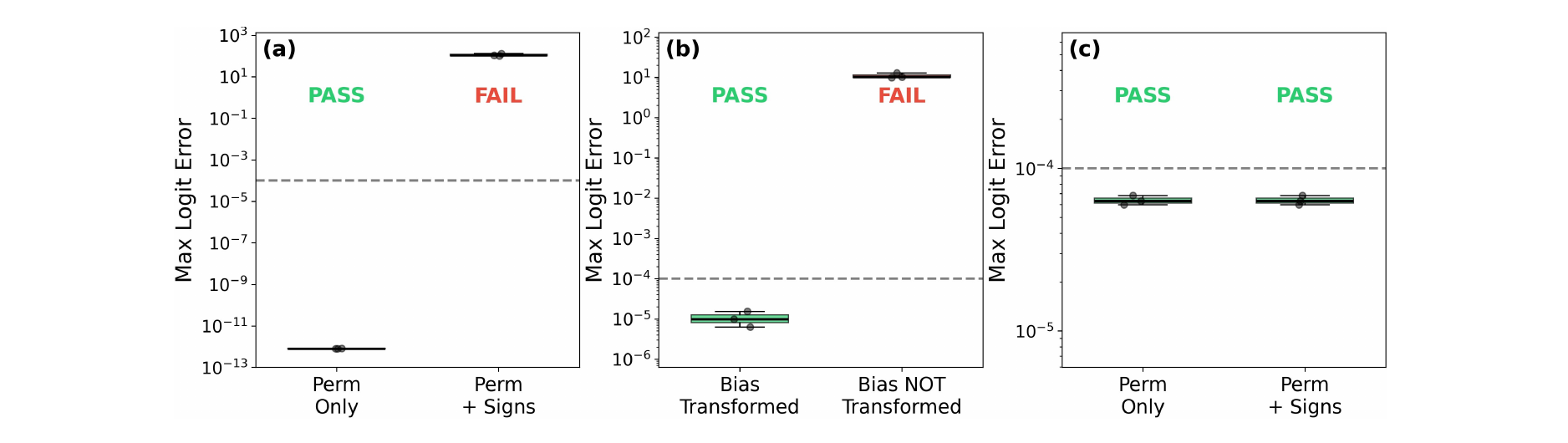
9 Proof of Theorem 2.1↩︎
Roadmap: we establish module-level gauge transform rules (norms, linear layers, attention), then compose them via residual addition and a layerwise induction to prove Theorem 1. We present the decoder-only case for concreteness, using the row-vector convention: residual activations \(H\in\mathbb{R}^{n\times d}\) are matrices with tokens as rows, and the gauge acts by right multiplication \(H^G=HG\).
Definition 1 (Gauge action). For permutation gauge \(G=P\in S_d\), \(P\) is a permutation matrix with \(P_{i,\pi(i)}=1\). For signed permutation gauge \(G=PS\in B_d\), additionally \(S=\operatorname{diag}(s_1,\ldots,s_d)\) with \(s_i\in\{-1,+1\}\). In both cases, the gauge action on residual activations \(H\in\mathbb{R}^{n\times d}\) is \(H^G:=HG\).
Lemma 2 (RMSNorm equivariance). Define \[\operatorname{RMSNorm}(h;\gamma)=\frac{h}{\sqrt{\frac{1}{d}\sum_i h_i^2+\epsilon}}\odot\gamma\] for row vector \(h\). With \(\gamma^G_j:=\gamma_{\pi^{-1}(j)}\) (permute only, no sign), we have \[\operatorname{RMSNorm}(hG;\gamma^G)=\operatorname{RMSNorm}(h;\gamma)\cdot G.\]
9.0.0.1 Proof.
Mean square is invariant under signed permutations: \(\frac{1}{d}\sum_i(hG)_i^2=\frac{1}{d}\sum_i h_i^2\). Thus \(\operatorname{RMS}(hG)=\operatorname{RMS}(h)\), so \(\operatorname{RMSNorm}(hG;\gamma^G)=hG/\operatorname{RMS}(h)\odot\gamma^G\). The permuted \(\gamma^G\) aligns elementwise scaling with the permuted coordinates, giving \((h/\operatorname{RMS}(h)\odot\gamma)G\).
9.0.0.2 Why \(\gamma\) permutes but does not flip signs.
The sign flip is absorbed into the activation \(h\), not \(\gamma\). Specifically, \((hG)_j=s_jh_{\pi^{-1}(j)}\) carries the sign, while \(\gamma^G_j=\gamma_{\pi^{-1}(j)}\) only permutes. The elementwise product \((hG\odot\gamma^G)_j=s_jh_{\pi^{-1}(j)}\gamma_{\pi^{-1}(j)}=s_j(h\odot\gamma)_{\pi^{-1}(j)}=((h\odot\gamma)G)_j\).
Lemma 3 (LayerNorm equivariance). Define \[\operatorname{LayerNorm}(h;\gamma,\beta)=\gamma\odot\frac{h-\mu(h)}{\sigma(h)}+\beta, \qquad \mu(h)=\frac{1}{d}\sum_i h_i.\] For permutation \(P\in S_d\) with \(\gamma^P_j=\gamma_{\pi^{-1}(j)}\) and \(\beta^P_j=\beta_{\pi^{-1}(j)}\), \[\operatorname{LayerNorm}(hP;\gamma^P,\beta^P)=\operatorname{LayerNorm}(h;\gamma,\beta)\cdot P.\] More generally, \(\epsilon P\) with \(\epsilon\in\{\pm1\}\) is equivariant if \(\beta^P\) is replaced by \(\epsilon\beta^P\). Signed permutations with nonconstant sign pattern are not equivariant in general.
9.0.0.3 Proof.
For permutation \(P\), \(\mu(hP)=\frac{1}{d}\sum_j(hP)_j=\frac{1}{d}\sum_j h_{\pi^{-1}(j)}=\mu(h)\). Thus \((hP-\mu(hP))=(h-\mu(h))P\) and LayerNorm is \(S_d\)-equivariant. For \(\epsilon=-1\), \(\mu(-hP)=-\mu(h)\) and the normalized centered vector changes by the same global sign, giving \[\operatorname{LayerNorm}(-hP;\gamma^P,-\beta^P)=\operatorname{LayerNorm}(h;\gamma,\beta)(-P).\] For signed permutation with nonconstant sign flips, \(\mu(hG)=\frac{1}{d}\sum_j s_jh_{\pi^{-1}(j)}\ne \pm\mu(h)\) in general. Thus \((hG-\mu(hG))\ne(h-\mu(h))G\), breaking equivariance.
Lemma 4 (Post-norm wrapper). Let \(G\) be an admissible gauge. Suppose \(\Delta\) is gauge-equivariant, \(\Delta^G(HG)=\Delta(H)G\), and \(N\) is gauge-equivariant, \(N^G(HG)=N(H)G\). Then \(\Phi(H)=N(H+\Delta(H))\) is gauge-equivariant: \(\Phi^G(HG)=\Phi(H)G\).
9.0.0.4 Proof.
\(\Phi^G(HG)=N^G(HG+\Delta^G(HG))=N^G((H+\Delta(H))G)=N(H+\Delta(H))G\).
Lemma 5 (Linear layer transforms under HuggingFace convention). HuggingFace Linear computes \(Y=XW^\top+b\) with \(W\in\mathbb{R}^{d_{\rm out}\times d_{\rm in}}\). Under gauge \(X^G=XG\):
READ (input from residual, output unchanged): set \(W^G=WG\), \(b^G=b\). Then \(Y^G=X^G(W^G)^\top+b^G=XGG^\top W^\top+b=XW^\top+b=Y\).
WRITE (output to residual): set \(W^G=G^\top W\), \(b^G=bG\). Then \(Y^G=X(W^G)^\top+b^G=XW^\top G+bG=(XW^\top+b)G=YG\).
Lemma 6 (Attention invariance). With \(Q,K,V\) projections as READ layers, the projected queries, keys, and values are unchanged under the gauge reparameterization. Therefore attention weights \(\operatorname{softmax}(QK^\top/\sqrt{d_k})\) are identical, and only the output projection (WRITE) produces a gauged residual contribution.
9.0.0.5 Proof.
Let \(H^G=HG\) be the gauged input to attention. Q-projection is READ: \(Q=HW_Q^\top+b_Q\) becomes \[Q^G=H^G(W_Q^G)^\top+b_Q=HGG^\top W_Q^\top+b_Q=HW_Q^\top+b_Q=Q.\] Similarly \(K^G=K\) and \(V^G=V\). \(Q/K/V\) biases are in head space, not residual space, so they remain unchanged under gauge. Therefore attention weights are unchanged. The O-projection is WRITE, producing \(\Delta^G=\Delta G\).
9.0.0.6 Proof of Theorem 1.
By induction on layers. Let \(H_\ell^G=H_\ell G\) at layer \(\ell\). Base case: token embeddings \(E=W_{\rm emb}[\mathrm{tokens}]\) are row vectors. With \(W_{\rm emb}^G=W_{\rm emb}G\), we have \(E^G=EG=H_0G\). For the inductive step, given \(H_\ell^G=H_\ell G\), let \(\Delta\) be the attention or MLP update. If the block is pre-norm, \(H'=H_\ell+\Delta(N(H_\ell))\); Lemma 2 or 3 and Lemma 6 (or Lemma 5 for MLP) give \(H'^G=H'G\). If post-norm, \(H'=N(H_\ell+\Delta(H_\ell))\); \(\Delta^G(H_\ell^G)=\Delta(H_\ell)G\) and Lemma 4 yields \(H'^G=H'G\). Applying this to attention and MLP gives \(H_{\ell+1}^G=H_{\ell+1}G\).
For the output, the LM head is READ from the final residual. With \(W_{\rm head}^G=W_{\rm head}G\), \[\operatorname{logits}^G=H_L^G(W_{\rm head}^G)^\top =H_LGG^\top W_{\rm head}^\top =H_LW_{\rm head}^\top =\operatorname{logits}.\] Tied embeddings: When \(W_{\rm head}=W_{\rm emb}\) (weight tying), both transform identically as \(W^G=WG\), preserving the tie. This is automatic since both are READ layers from/to the residual stream.
Two constraints determine the gauge group. For RMSNorm, the diagonal learned gain \(\gamma\) must remain diagonal under gauge. For a generic gain vector, or a jointly generic family of gain vectors sharing a residual chart, the simultaneous stabilizer in \(O(d)\) is exactly the signed permutation group \(B_d\). Exact tied coordinates across all relevant gains can admit block-orthogonal stabilizers, but these do not preserve sparse coordinate identity; all results use the always-present \(B_d\) subgroup. For LayerNorm, mean-centering breaks independent sign symmetry. For signed permutation \(G\) with signs \(s_i\), the mean \(\mu(xG)=\frac{1}{d}\sum_j s_jx_{\pi^{-1}(j)}\) generally differs from \(\pm\mu(x)\) unless all signs are equal. Thus generic affine LayerNorm admits \(\{\pm P:P\in S_d\}\), where the negative component requires \(\beta\mapsto-\beta P\); its per-index relabeling content is \(S_d\). Both groups are large: \(|S_d|=d!\) and \(|B_d|=d!\cdot 2^d\). The factor of \(2^d\) distinguishes the architectures, but both imply neuron indices are non-identifiable without fixing a gauge.
Remark 9 (Generic \(\gamma\) and practical degeneracies). For RMSNorm \(\operatorname{RMSNorm}(x)=x/\left\lVert x \right\rVert\odot\gamma\), the admissible gauge \(G\) must preserve diagonality under conjugation: \(G^\top\operatorname{diag}(\gamma)G\) remains diagonal (possibly permuted). For generic \(\gamma\) (distinct entries), the only orthogonal matrices with this property are signed permutations, i.e., \(B_d\); if \(\gamma_i=\gamma_j\) for some \(i\ne j\), a single RMSNorm layer also admits rotations within the equal-\(\gamma\) subspace.
Exact repeats in learned \(\gamma\) can occur in real checkpoints, especially in low-precision formats such as bf16/fp16, which can enlarge the admissible symmetry beyond \(B_d\) for a given RMSNorm layer. For a transformer-wide residual chart, the continuous part is the intersection of these per-layer stabilizers across all RMSNorms sharing the chart. We do not rely on this enlargement; all results use the always-present discrete subgroup \(B_d\).
Algorithm behavior with continuous symmetry: Our activation-based alignment (§3) selects one representative from the equivalence class—specifically, the discrete signed permutation that maximizes activation cross-correlation. Within equal-\(\gamma\) subspaces where continuous rotations are valid, this representative is determined by the probe activations and assignment tie-breaking. This choice is reproducible for a fixed probe set even when the underlying symmetry group is larger than \(B_d\). Similarly, for LayerNorm with repeated \((\gamma_i,\beta_i)\) pairs, additional permutations within tied subspaces are valid.
10 Proof of atlas consistency↩︎
10.0.0.1 Proof of Proposition 6.
If \(\hat{G}_{ij}=R_i^{-1}R_j\), then every cycle product telescopes: \[\hat{G}_{i_1i_2}\hat{G}_{i_2i_3}\cdots\hat{G}_{i_ki_1} =R_{i_1}^{-1}R_{i_2}R_{i_2}^{-1}\cdots R_{i_k}^{-1}R_{i_1} =I.\] Conversely, fix a root \(r\). For any vertex \(i\), choose a path from \(r\) to \(i\) and define \(R_i\) as the ordered product of edge labels along that path. Zero holonomy makes \(R_i\) path-independent: two paths from \(r\) to \(i\) form a cycle after reversing one path, so their products agree. For an edge \((i,j)\), the path to \(i\) followed by that edge is a path to \(j\); path-independence therefore gives \(R_j=R_i\hat{G}_{ij}\), hence \(\hat{G}_{ij}=R_i^{-1}R_j\).
11 Proofs for artifact covariance↩︎
11.0.0.1 Proof of Proposition 3.
The parameter map \(T_G\) is modulewise multiplication by fixed matrices \(G\), \(G^\top\), or by the corresponding permutation of norm gains. Hence it is affine in the base parameters and linear on increments: \[T_G(\theta+\Delta\theta)-T_G(\theta)=T_G^{\rm lin}(\Delta\theta).\] For a LoRA update \(\Delta W=BA\), the READ rule is \(\Delta W^G=\Delta WG=B(AG)\), so \(A^G=AG\), \(B^G=B\). The WRITE rule is \(\Delta W^G=G^\top\Delta W=(G^\top B)A\), so \(A^G=A\), \(B^G=G^\top B\).
11.0.0.2 Proof of Corollary 1.
Write \(G=PS\), with \(S=\operatorname{diag}(s)\). Let \(M=\Delta WP\). Then \[\left\lVert \Delta WPS-\Delta WP \right\rVert_F^2 =\left\lVert MS-M \right\rVert_F^2 =\sum_j(s_j-1)^2\left\lVert M_{:,j} \right\rVert_2^2 =4\sum_{j:s_j=-1}\left\lVert (\Delta WP)_{:,j} \right\rVert_2^2.\] Since \(P\) is orthogonal, \(\sum_j\left\lVert (\Delta WP)_{:,j} \right\rVert_2^2=\left\lVert \Delta W \right\rVert_F^2\). Under iid uniform signs, each column contributes with probability \(1/2\), giving \(2\left\lVert \Delta W \right\rVert_F^2\) in expectation.
11.0.0.3 Proof of Lemma 1.
The norm identity is the vector version of the preceding proof with \(m=vP\): \[\left\lVert vG-vP \right\rVert_2^2=\left\lVert mS-m \right\rVert_2^2 =4\sum_{j:s_j=-1}m_j^2.\] The cosine follows from \(\left\langle vG,vP \right\rangle=\left\langle mS,m \right\rangle=\sum_j s_jm_j^2\) and \(\left\lVert vG \right\rVert_2=\left\lVert vP \right\rVert_2=\left\lVert m \right\rVert_2\).
12 Proofs for decomposition and matching ceiling↩︎
12.0.0.1 Proof of Theorem 2.
For any signed permutation \(P\in B_d\), \[\left\lVert Q-P \right\rVert_F^2=\left\lVert Q \right\rVert_F^2+\left\lVert P \right\rVert_F^2-2\operatorname{tr}(Q^\top P)=2d-2\operatorname{tr}(Q^\top P),\] so minimizing Frobenius distance is equivalent to maximizing \(\operatorname{tr}(Q^\top P)\). Write \(P\) as a permutation \(\sigma\) plus signs \(\epsilon_j\in\{\pm1\}\), with column \(j\) mapped to row \(\sigma(j)\). Then \[\operatorname{tr}(Q^\top P)=\sum_j \epsilon_jQ_{\sigma(j),j}.\] For a fixed \(\sigma\), the optimal sign is \(\epsilon_j=\operatorname{sign}(Q_{\sigma(j),j})\), giving objective \(\sum_j |Q_{\sigma(j),j}|\). Maximizing this over permutations is exactly a linear assignment problem on \(|Q|\). Generically the assignment has a unique maximizer; ties are the only source of non-uniqueness. Since both \(Q\) and \(P^\star\) are orthogonal, \(R=Q(P^\star)^{-1}\) is orthogonal. Finally, \[\left\lVert R-I \right\rVert_F=\left\lVert Q(P^\star)^{-1}-I \right\rVert_F=\left\lVert Q-P^\star \right\rVert_F\] by right-invariance of the Frobenius norm. The scalar \(\rho(Q)=d^{-1}\operatorname{tr}(Q^\top P^\star)\) is one iff \(Q=P^\star\in B_d\) by the distance identity above. For Haar-random \(Q\), the largest entry in each column is \(O(\sqrt{\log d/d})\) in expectation, and assignment can improve constants but not order, giving \(\mathbb{E}\rho(Q)=O(\sqrt{\log d/d})\).
12.0.0.2 Proof of Theorem 4.
Let the target columns satisfy \(v_{\pi^\star(i)}=s_i^\star u_i\) in population, up to sampling noise, and assume \(\mathbb{E}[u_iu_j]=0\) for \(i\ne j\) with variance \(\sigma_i^2>0\) on coordinate \(i\). Assignment is unchanged by positive rescaling, so work with the empirical covariance \(\widehat C=N^{-1}H_s^\top H_t\), which obeys \[\widehat C_{i,j}\xrightarrow[N\to\infty]{}s_i^\star\sigma_i^2\mathbf{1}\{j=\pi^\star(i)\}.\] All off-diagonal entries vanish in population. If \(s_i^\star=+1\), the correct entry is the unique positive entry in row \(i\), so signed-correlation maximization can select it. If \(s_i^\star=-1\), the correct entry is the most negative population entry in its row, while all incorrect entries are zero; a maximizer of \(\sum_i C_{i,\pi(i)}\) therefore avoids that entry whenever an off-diagonal assignment is available. Hungarian’s global one-to-one constraint must displace some other row in exchange: when there are \(k\ge2\) negative signs, swapping any two negative-sign rows yields strict gain \(\sigma_{i_1}^2+\sigma_{i_2}^2>0\) over the truth, so the maximizer strictly avoids all \(k\) negatives. The event \(k\le1\) has probability \(O(d2^{-d})\) under iid uniform signs. Hence signed-correlation matching has limiting accuracy equal to the positive-sign fraction except on this event, giving expectation \(1/2+O(d2^{-d})\) under independent uniform signs.
By contrast, \(|\widehat C_{i,\pi^\star(i)}|\to\sigma_i^2>0\) and \(|\widehat C_{i,j}|\to0\) for \(j\ne\pi^\star(i)\). Under standard sub-Gaussian probe assumptions, concentration plus a union bound gives \(\left\lVert \widehat C-C \right\rVert_\infty=O(\sqrt{\log d/N})\); if this perturbation is smaller than the assignment margin, Lemma 8 preserves the true assignment. Thus sign-marginalized matching converges to the true permutation.
12.1 FFN hidden unit symmetry↩︎
The residual gauge acts on the \(d\)-dimensional residual stream. MLP hidden units live in a separate \(d_{\rm ffn}\)-dimensional space. We first show that FFN hidden activations are invariant under the residual gauge, then prove they admit their own independent permutation symmetry.
12.1.0.1 Proof.
For a plain 2-layer FFN, let \(\Delta_{\rm MLP}(H)=\sigma(HW_{\rm up}^\top+b_{\rm up})W_{\rm down}^\top+b_{\rm down}\) under row-vector convention. Under the residual gauge, \(W_{\rm up}\) is READ, \(W_{\rm up}^G=W_{\rm up}G\), \(b_{\rm up}^G=b_{\rm up}\); \(W_{\rm down}\) is WRITE, \(W_{\rm down}^G=G^\top W_{\rm down}\), \(b_{\rm down}^G=b_{\rm down}G\). The preactivation into the hidden units is \[Z^G=H^G(W_{\rm up}^G)^\top+b_{\rm up}^G =(HG)(W_{\rm up}G)^\top+b_{\rm up} =HG G^\top W_{\rm up}^\top+b_{\rm up} =HW_{\rm up}^\top+b_{\rm up}=Z.\] Since \(\sigma\) is elementwise, \(A^G=\sigma(Z^G)=\sigma(Z)=A\). The hidden activations are literally identical.
Gated MLP (Llama/SwiGLU). For \(\Delta_{\rm MLP}(H)=(\sigma(HW_{\rm gate}^\top+b_{\rm gate})\odot(HW_{\rm up}^\top+b_{\rm up}))W_{\rm down}^\top+b_{\rm down}\): Both \(W_{\rm gate}\) and \(W_{\rm up}\) are READ layers, so the same \(GG^\top=I\) cancellation applies to both branches. Thus both the gated and linear pre-activations are unchanged, their Hadamard product is unchanged, and the hidden activations are invariant.
Output equivariance. The down-projection is WRITE, so: \[\Delta_{\rm MLP}^G=A(W_{\rm down}^G)^\top+b_{\rm down}^G =A(G^\top W_{\rm down})^\top+b_{\rm down}G =AW_{\rm down}^\top G+b_{\rm down}G =\Delta_{\rm MLP}\cdot G.\] The FFN contribution is equivariant (picks up \(G\) on output), while internal hidden activations are invariant.
Corollary 2. Methods that output top-\(k\) FFN hidden unit indices (e.g., “knowledge neurons”) are gauge-variant under the FFN symmetry (\(S_{d_{\rm ffn}}\) for plain FFNs, \(B_{d_{\rm ffn}}\) for gated FFNs), but are not affected by the residual gauge \(G\). Thus such methods require gauge-fixing for the FFN symmetry, which is independent of the residual-stream symmetry analyzed in our main theorems.
Theorem 10 (FFN permutation symmetry). For each FFN (MLP) layer with intermediate dimension \(d_{\rm ffn}\) and elementwise activation \(\sigma\), the permutation group \(S_{d_{\rm ffn}}\) acts on the hidden unit indices while leaving the layer output invariant. Specifically, for \(P\in S_{d_{\rm ffn}}\), define \[W'_{\rm up}=P^\top W_{\rm up},\quad b'_{\rm up}=b_{\rm up}P,\qquad W'_{\rm down}=W_{\rm down}P,\quad b'_{\rm down}=b_{\rm down}.\] Then \(\operatorname{FFN}'(x)=\operatorname{FFN}(x)\) for all inputs \(x\). For gated FFNs (Llama/SwiGLU), the same permutation \(P\) applies to both branches: \(W'_{\rm gate}=P^\top W_{\rm gate}\) and \(b'_{\rm gate}=b_{\rm gate}P\). For plain (non-gated) FFNs, sign flips are not a symmetry because common activations (GELU, SiLU, ReLU) are not odd functions. Gated FFNs admit additional sign symmetry; see Proposition 11.
12.1.0.2 Proof.
Let \(\operatorname{FFN}(x)=\sigma(xW_{\rm up}^\top+b_{\rm up})W_{\rm down}^\top+b_{\rm down}\) (row-vector convention), with \(W_{\rm up}\in\mathbb{R}^{d_{\rm ffn}\times d_{\rm model}}\) and \(W_{\rm down}\in\mathbb{R}^{d_{\rm model}\times d_{\rm ffn}}\).
Define the hidden activations \(h:=\sigma(xW_{\rm up}^\top+b_{\rm up})\in\mathbb{R}^{1\times d_{\rm ffn}}\). With the transformed weights: \[(W'_{\rm up})^\top=(P^\top W_{\rm up})^\top=W_{\rm up}^\top P\] so the new preactivation is: \[x(W'_{\rm up})^\top+b'_{\rm up}=xW_{\rm up}^\top P+b_{\rm up}P=(xW_{\rm up}^\top+b_{\rm up})P.\] Since \(\sigma\) is elementwise, it commutes with coordinate permutations: \[h'=\sigma((xW_{\rm up}^\top+b_{\rm up})P)=\sigma(xW_{\rm up}^\top+b_{\rm up})P=hP.\] For the output: \[(W'_{\rm down})^\top=(W_{\rm down}P)^\top=P^\top W_{\rm down}^\top\] so: \[y'=h'(W'_{\rm down})^\top+b_{\rm down}=(hP)(P^\top W_{\rm down}^\top)+b_{\rm down}=h(PP^\top)W_{\rm down}^\top+b_{\rm down}.\] Since \(P\) is a permutation matrix, \(PP^\top=I\), so \(y'=hW_{\rm down}^\top+b_{\rm down}=y\).
Proposition 11 (Signed-permutation subgroup of gated FFNs). For gated FFNs (SwiGLU/GLU as in Llama/Mistral/Qwen), \(B_{d_{\rm ffn}}\) is an exact orthogonal hidden-coordinate symmetry subgroup, not merely \(S_{d_{\rm ffn}}\).
For \(P\in S_{d_{\rm ffn}}\) and \(S=\operatorname{diag}(s_1,\ldots,s_{d_{\rm ffn}})\), define \[\begin{align} &W'_{\rm gate}=P^\top W_{\rm gate},\quad b'_{\rm gate}=b_{\rm gate}P,\quad W'_{\rm up}=SP^\top W_{\rm up},\quad b'_{\rm up}=b_{\rm up}PS,\\ &W'_{\rm down}=W_{\rm down}PS,\quad b'_{\rm down}=b_{\rm down}. \end{align}\] Then \(\operatorname{FFN}'(x)=\operatorname{FFN}(x)\) for all \(x\), and the post-gating hidden vector transforms as \(A'(x)=A(x)PS\).
12.1.0.3 Proof.
Let \(u(x)=xW_{\rm up}^\top+b_{\rm up}\) (linear branch) and \(g(x)=xW_{\rm gate}^\top+b_{\rm gate}\) (gate branch). Under the transform: \[\begin{align} u'(x)&=x(W'_{\rm up})^\top+b'_{\rm up}\\ &=x(SP^\top W_{\rm up})^\top+b_{\rm up}PS\\ &=(xW_{\rm up}^\top+b_{\rm up})PS=u(x)PS, \end{align}\] and \(g'(x)=g(x)P\), hence \(\sigma(g'(x))=\sigma(g(x))P\) since \(\sigma\) is elementwise. The post-gating hidden vector becomes: \[A'(x)=\sigma(g'(x))\odot u'(x)=(\sigma(g(x))P)\odot(u(x)PS)=(\sigma(g(x))\odot u(x))PS=A(x)PS.\] For the output: \[\begin{align} \operatorname{FFN}'(x)&=A'(x)(W'_{\rm down})^\top+b_{\rm down}\\ &=A(x)PS(W_{\rm down}PS)^\top+b_{\rm down}\\ &=A(x)W_{\rm down}^\top+b_{\rm down}=\operatorname{FFN}(x), \end{align}\] since \(PS\) is orthogonal and \((PS)(PS)^\top=I\).
Remark 12 (Additional diagonal scaling in gated FFNs). The signed-permutation subgroup is not the full parameter symmetry of a gated FFN. For any invertible diagonal \(D\) in hidden space, the transform \(W'_{\rm up}=DW_{\rm up}\), \(b'_{\rm up}=b_{\rm up}D\), \(W'_{\rm down}=W_{\rm down}D^{-1}\), with the gate branch unchanged, also preserves the FFN function. This larger scaling symmetry is non-orthogonal unless \(D\) has \(\pm1\) diagonal entries, so it is separate from the residual-stream coordinate-preserving group studied in the main text.
Remark 13 (Why Gated FFNs Admit Sign Flips). The key point is that the hidden-unit sign matrix acts on the linear* branch \(u(x)\) (via \(W_{\rm up}\)), not inside the nonlinear gate \(\sigma(g(x))\). Although \(\sigma\) (SiLU/GELU) is not odd, the sign acts on \(u(x)\) which is then multiplied by \(\sigma(g(x))\). This is distinct from plain FFNs where the nonlinearity directly acts on the pre-activation.*
Remark 14 (Independence of Symmetries). The residual gauge \(G\in B_d\) and FFN hidden transform act on orthogonal index sets and can be applied simultaneously. The residual gauge acts on the \(d_{\rm model}\) columns of \(W_{\rm up}\); the FFN hidden transform acts on the \(d_{\rm ffn}\) rows. For the signed hidden subgroup, write \(K=PS\). The combined transform is: \[W_{\rm gate}^{G,P}=P^\top W_{\rm gate}G,\qquad W_{\rm up}^{G,K}=K^\top W_{\rm up}G,\qquad W_{\rm down}^{G,K}=G^\top W_{\rm down}K.\] Biases transform as \(b_{\rm gate}\mapsto b_{\rm gate}P\), \(b_{\rm up}\mapsto b_{\rm up}K\), and \(b_{\rm down}\mapsto b_{\rm down}G\). These commute because \(G\) and \(K\) act on disjoint dimensions: \(G\) permutes/signs the \(d\)-dimensional residual space while \(K\) acts on the \(d_{\rm ffn}\)-dimensional hidden space.
Remark 15 (Why Plain (Non-Gated) FFNs Have No Sign Symmetry). For plain 2-layer MLPs of the form \(h=\sigma(xW_{\rm up}^\top+b)\), sign flips would require \(\sigma(-z)=-\sigma(z)\) (oddness). \(\operatorname{ReLU}(x)=\max(0,x)\) satisfies \(\operatorname{ReLU}(-x)\ne-\operatorname{ReLU}(x)\) for \(x>0\); similarly GELU and SiLU are not odd. Thus for plain* FFNs, sign flips do not preserve outputs, limiting the orthogonal hidden-coordinate subgroup to \(S_{d_{\rm ffn}}\). Plain ReLU FFNs also have the familiar positive diagonal scaling symmetry from ReLU homogeneity; GELU/SiLU plain FFNs generally do not. Gated FFNs (Proposition 11) admit this because the sign matrix acts on the linear branch while the nonlinear gate branch is only permuted.*
12.2 SAE gauge invariance↩︎
Sparse autoencoders (SAEs) learn feature dictionaries from residual-stream activations. We show that the SAE training objective is invariant under residual gauge, so SAEs cannot canonically choose a basis.
Proposition 16 (SAE objective is gauge-invariant). Let \(D=\{h_i\}_{i=1}^N\subset\mathbb{R}^d\) be residual activations (row-vector convention), and consider an SAE with encoder and decoder \[z(h)=\phi(hW_{\rm enc}^\top+b_{\rm enc}),\qquad \hat{h}(h)=z(h)W_{\rm dec}^\top+b_{\rm dec},\] trained with objective \[L(\theta;D)=\sum_{h\in D}\left\lVert h-\hat{h}(h) \right\rVert_2^2+\lambda\left\lVert z(h) \right\rVert_1.\] Let \(G\) be any admissible residual gauge (a permutation, possibly composed with the global sign flip, for LayerNorm models, or a signed permutation for RMSNorm models), and define \(D^G=\{hG:h\in D\}\) and parameters \[W_{\rm enc}^G=W_{\rm enc}G,\quad b_{\rm enc}^G=b_{\rm enc},\quad W_{\rm dec}^G=G^\top W_{\rm dec},\quad b_{\rm dec}^G=b_{\rm dec}G.\] Then for all \(h\in D\), \[z^G(hG)=z(h),\qquad \hat{h}^G(hG)=\hat{h}(h)G,\] and consequently \(L(\theta^G;D^G)=L(\theta;D)\).
12.2.0.1 Proof.
Using \(GG^\top=I\), \(z^G(hG)=\phi(hGG^\top W_{\rm enc}^\top+b_{\rm enc})=z(h)\). Then \(\hat{h}^G(hG)=z(h)W_{\rm dec}^\top G+b_{\rm dec}G=\hat{h}(h)G\). Thus \((hG-\hat{h}^G(hG))=(h-\hat{h}(h))G\), so the squared error is preserved because \(G\) is orthogonal, and the \(\ell_1\) term is unchanged because \(z^G(hG)=z(h)\).
Corollary 3 (SAE feature indices are non-identifiable). Independently of the residual gauge, for any feature permutation \(P\in S_{d_{\rm feat}}\), the SAE objective is invariant under \(W_{\rm enc}\mapsto P^\top W_{\rm enc}\), \(b_{\rm enc}\mapsto b_{\rm enc}P\), and \(W_{\rm dec}\mapsto W_{\rm dec}P\), with \(b_{\rm dec}\) unchanged. Thus SAE feature indices are non-canonical without alignment.
13 Transform rules for all module types↩︎
All rules use the row-vector convention: \(H^G=HG\) where \(H\) has shape \([n,d]\). HuggingFace Linear computes \(Y=XW^\top+b\) with \(W\in\mathbb{R}^{d_{\rm out}\times d_{\rm in}}\).
| Module | Type | Weight | Bias |
|---|---|---|---|
| Tok/Pos embed | Embed | \(W\mapsto WG\) | – |
| Q, K, V proj | READ | \(W\mapsto WG\) | unchanged |
| O projection | WRITE | \(W\mapsto G^\top W\) | \(b\mapsto bG\) |
| MLP up/gate | READ | \(W\mapsto WG\) | unchanged |
| MLP down | WRITE | \(W\mapsto G^\top W\) | \(b\mapsto bG\) |
| RMSNorm | Norm | \(\gamma\mapsto\gamma[\pi^{-1}]\) | – |
| LayerNorm | Norm | \(\gamma\mapsto\gamma[\pi^{-1}]\) | \(\beta\mapsto\epsilon\beta[\pi^{-1}]\) for \(G=\epsilon P\); other signs break |
| LM head | READ | \(W\mapsto WG\) | – |
Index form: let \(\pi\) be the permutation with \(P_{i,\pi(i)}=1\), and \(s_j\) the signs. READ maps satisfy \(W^G[:,j]=s_jW[:,\pi^{-1}(j)]\) (permute/sign columns). WRITE maps satisfy \(W^G[i,:]=s_iW[\pi^{-1}(i),:]\) (permute/sign rows). WRITE bias transforms as \(b_j^G=s_jb_{\pi^{-1}(j)}\). RMSNorm transforms as \(\gamma_j^G=\gamma_{\pi^{-1}(j)}\) (permute only, no sign).
13.0.0.1 Why \(Q,K,V\) are unchanged under reparameterization.
This is the key insight that makes the proof work with multi-head attention. With \(H^G=HG\) and \(W_Q^G=W_QG\) (READ rule): \[Q^G=H^G(W_Q^G)^\top=HG\cdot G^\top W_Q^\top=HW_Q^\top=Q.\] The gauge cancels at the READ boundary, so attention patterns are identical.
14 Hungarian optimality↩︎
The sign-marginalized cost is optimal for recovering signed permutations. Let \(u_i\) be column \(i\) of \(H\), \(v_j\) column \(j\) of \(H^G\), and \(C=H^\top H^G\). We seek a permutation \(\pi\) and signs \(s\) minimizing \[\min_{\pi\in S_d,\;s\in\{\pm1\}^d}\sum_{i=1}^d\left\lVert u_i-s_iv_{\pi(i)} \right\rVert_2^2.\] Expanding by columns, \[\sum_{i=1}^d\left\lVert u_i-s_iv_{\pi(i)} \right\rVert_2^2 =\sum_i\left(\left\lVert u_i \right\rVert_2^2+\left\lVert v_{\pi(i)} \right\rVert_2^2-2s_i u_i^\top v_{\pi(i)}\right) =\mathrm{const}-2\sum_i s_iC_{i,\pi(i)}.\] For any fixed permutation \(\pi\), the optimal sign is \(s_i=\operatorname{sign}(C_{i,\pi(i)})\), yielding \[\max_{\pi\in S_d}\sum_i |C_{i,\pi(i)}|.\] This is exactly a linear assignment problem on cost \(-|C_{i,j}|\), solvable by the Hungarian algorithm.
14.1 Assignment stability under a margin↩︎
Lemma 8 (Assignment stability under a margin). Let \(C\in\mathbb{R}^{d\times d}\) and define \(F_C(\pi)=\sum_{i=1}^d |C_{i,\pi(i)}|\) for \(\pi\in S_d\). Assume the maximizer \(\pi^\star=\operatorname*{arg\,max}_\pi F_C(\pi)\) is unique and define the margin \[m:=F_C(\pi^\star)-\max_{\pi\ne\pi^\star}F_C(\pi)>0.\] If \(E\in\mathbb{R}^{d\times d}\) satisfies \(\left\lVert E \right\rVert_\infty=\max_{i,j}|E_{i,j}|\le\epsilon\) and \(2d\epsilon<m\), then \(\pi^\star\) remains the unique maximizer for \(C+E\).
14.1.0.1 Proof.
For any scalars \(a,b\), \(||a+b|-|a||\le |b|\). Thus for any \(\pi\), \[|F_{C+E}(\pi)-F_C(\pi)| \le\sum_{i=1}^d |E_{i,\pi(i)}| \le d\epsilon.\] Therefore \(F_{C+E}(\pi^\star)\ge F_C(\pi^\star)-d\epsilon\) and for any \(\pi\ne\pi^\star\), \(F_{C+E}(\pi)\le F_C(\pi)+d\epsilon\le F_C(\pi^\star)-m+d\epsilon\). Hence \(F_{C+E}(\pi^\star)-F_{C+E}(\pi)\ge m-2d\epsilon>0\).
15 Experimental details↩︎
15.0.0.1 Models.
Across experiments we use 11 models spanning 4 architectures and scales from \(\sim\)10M to 8B parameters. The symmetry-boundary checks of Table 2 use the seven models listed there; the transport, optimizer-state, LoRA, steering, SAE, and merging experiments add four further RMSNorm models.
15.0.0.2 Production-scale RMSNorm models.
Qwen2.5-7B has 28 layers, \(d=3584\), RMSNorm, and Q/K/V head-space biases only (boundary check). Llama-3.1-8B has 32 layers, \(d=4096\), RMSNorm, and no biases (boundary check). Llama-2-7b-chat-hf has 32 layers, \(d=4096\), RMSNorm, and no biases (boundary check, refusal reanalysis, gauge-scramble merge).
15.0.0.3 Mid-scale RMSNorm models.
TinyLlama-1.1B has 22 layers, \(d=2048\), RMSNorm, and no biases (boundary check, SAE/steering/LoRA transfer). Qwen2.5-1.5B has 28 layers, \(d=1536\), RMSNorm, and Q/K/V head-space biases only (transport trajectory recovery, \(B_d\)/\(S_d\) steering, LoRA, gauge-scramble). Qwen2.5-0.5B has 24 layers, \(d=896\), RMSNorm, and Q/K/V head-space biases only (stateful optimizer resumption). Llama-3.2-1B has 16 layers, \(d=2048\), RMSNorm, and no biases (transport replication, steering replication; Appendix 17). Qwen Q/K/V biases live in attention head space and remain unchanged under the residual gauge, as in Lemma 6; the reported transform rules do not rely on residual-space WRITE biases in these modules.
15.0.0.4 Small-scale and other architectures.
We use a custom 10M Llama-style transformer with 4 layers, \(d=256\), RMSNorm (independent-seed merging; trained from scratch on identical data, different seeds); BERT-base (110M, 12 layers, \(d=768\), LayerNorm; \(S_d\) per-index symmetry; boundary check); T5-small (60M, 6+6 layers, \(d=512\), T5LayerNorm; \(B_d\) symmetry; boundary check); and ViT-B/16 (86M, 12 layers, \(d=768\), LayerNorm; \(S_d\) per-index symmetry; boundary check).
15.0.0.5 Existing assets and licenses.
All external checkpoints and datasets are used through their original public distributions and are not redistributed with this paper. The Qwen2.5, TinyLlama, BERT-base, T5-small, and ViT checkpoints report Apache-2.0 license metadata on their Hugging Face model cards; Meta Llama checkpoints are gated and used under the corresponding Llama 2, Llama 3.1, or Llama 3.2 community license terms. WikiText is used under its CC-BY-SA-3.0/GFDL license metadata; SST-2/GLUE is used through the public GLUE distribution and original benchmark terms. ParaRel prompt templates used by the knowledge-neuron audit scripts are credited to Elazar et al. [2021]. Arditi et al.’s refusal-direction code and splits are credited in Appendix 15.3 and used only for the replication/audit reported there. Core software dependencies are PyTorch, Hugging Face Transformers/Datasets [Wolf et al., 2020], NumPy, and SciPy; their standard open-source licenses are BSD-style or Apache-2.0, and SciPy’s assignment solver is cited where used.
15.0.0.6 Gauge transforms.
We generate random gauges using NumPy with deterministic seeds: the permutation is a random permutation of \([0,d-1]\) with seed \(s\); the signs are a random choice from \(\{-1,+1\}^d\) with seed \(s+1000\); multi-gauge sweeps use seeds 42–61 (\(K=20\) gauges). All transforms are applied in-place to minimize memory overhead.
15.0.0.7 Steering vectors.
We extract sycophancy steering vectors using Contrastive Activation Addition (CAA): generate contrastive prompt pairs (sycophantic vs. honest responses), extract residual stream activations at layer 10, and compute the mean difference vector across prompt pairs. Steering effect is measured as the logit difference change when adding the vector at inference.
15.0.0.8 Evaluation metrics.
Logit invariance is evaluated on a fixed invariance batch (5 short prompts for language models; 5 random images for ViT), and we report the maximum absolute logit deviation across the batch. This batch is separate from the alignment probe set used for Hungarian gauge recovery. The logit error is the maximum absolute difference in output logits between original and gauge-transformed models, with threshold \(\sim10^{-4}\) for gauge invariance. Top-\(k\) overlap counts shared indices between top-\(k\) coordinates by activation magnitude with \(k=10\). Linear CKA uses standard centering across samples (HSIC with linear kernel), i.e., \[\operatorname{CKA}(X,Y)=\frac{\left\lVert X_c^\top Y_c \right\rVert_F^2}{\left\lVert X_c^\top X_c \right\rVert_F\left\lVert Y_c^\top Y_c \right\rVert_F},\] where \(X_c,Y_c\) are centered across samples.
15.0.0.9 Refusal direction reanalysis (Arditi et al., 2024).
Setup. We reproduce Arditi et al.’s released pipeline on meta-llama/Llama-2-7b-chat-hf (full protocol in Appendix 15.3). Candidates. We form directions \(r^{(\ell)}_i=\mathbb{E}[h^{(\ell)}_i\mid\mathrm{harmful}]-\mathbb{E}[h^{(\ell)}_i\mid\mathrm{harmless}]\) from block-input residual streams. Selection. We follow their bypass/induce criterion with KL filter 0.1
and layer cutoff \(\ell<0.8L\); refusal score is last-token log-odds on \(R=\{306\}\). Checks. On 20 harmful validation prompts (greedy decoding), ablating the selected
direction reduces refusal from 20/20 to 3/20. We match their released direction artifact (layer 14, position \(-1\)) with cosine 0.984 in the same residual space (\(d=4096\)).
15.0.0.10 Hungarian alignment.
The sign-marginalized recovery procedure uses SciPy’s linear sum assignment solver [Virtanen et al., 2020]; SciPy documents this routine as a modified Jonker–Volgenant implementation described by Crouse [2016], building on shortest-augmenting-path assignment algorithms [Jonker and Volgenant, 1987]. Our gauge-derived cost matrices are near-permutation, and the dense assignment step completes in a few seconds for \(d=4096\) in our implementation (worst-case \(O(d^3)\)). For \(d\ge 8192\), we restrict each row to its top-\(m\) matches in \(|C|\) (we use \(m=200\)) and greedily match; this avoids cubic assignment but still forms the dense cross-correlation \(C=H_{\mathrm{orig}}^{\top}H_{\mathrm{gauged}}\). On a \(d=4096\) ablation, greedy top-200 recovers 94.7% permutation / 97.5% sign vs 100% exact. Probe set: 30 diverse sentences totaling \(\sim\)500 tokens. Evaluation uses held-out test sentences (disjoint from probe set).
15.0.0.11 Reproducibility.
Unless otherwise stated, evaluation and gauge-recovery experiments load models in float32 for numerical stability. The Qwen LoRA row uses a bf16-trained adapter; all raw, \(S_d\), \(B_d\), and reference evaluations for that row use the same trained checkpoint precision, so the comparison isolates gauge transport rather than dtype. All random seeds are fixed and reported. JSON result files include full
hyperparameters and timestamps. For transport experiments, we enable deterministic CUDA algorithms (torch.use_deterministic_algorithms) to ensure exact reproducibility of composed gauge estimates; this disables TF32 and may reduce speed.
15.1 Compute resources↩︎
All reported experiments are single-worker PyTorch jobs, with no model parallelism, data parallelism, or distributed training. Exact float32 7B/8B boundary and recovery rows require a CUDA GPU with at least 48 GB VRAM; half-precision variants fit on 24 GB-class GPUs but are not the exact rows. The 7B/8B gradient-times-activation attribution sweep used a single H200 worker. The 1B–1.5B evaluation, LoRA, TinyLlama tool-transfer, Qwen2.5-1.5B transport, and Llama-3.2-1B transport runs fit on one 24 GB-class GPU. We recommend 100–300 GB local disk for Hugging Face caches and temporary checkpoints.
The archived timers for the transport families alone sum to about 154 single-GPU hours. Including the shorter un-timed boundary, merge, LoRA/SAE, attribution, and optimizer-state runs, a from-scratch reproduction of all reported tables should budget roughly 200–250 single-GPU hours, plus model-download time.
| Result family | Worker and memory | Run time / run size |
|---|---|---|
| Symmetry-boundary, gauge-fixing, and attribution audits | Single CUDA worker. Float32 7B/8B rows require \(\geq\)48 GB VRAM; H200 used for the 7B/8B grad\(\times\)act attribution sweep. Smaller models fit on 24 GB-class GPUs. | Boundary/gauge recovery uses 5–30 prompts. Budget tens of minutes per 7B/8B model, dominated by loading and forward/backward passes. |
| Qwen2.5-1.5B transport and steering transfer | Single CUDA worker, float32. The archived 200-step log records about 6.2 GB allocated after model load and about 6.2–6.3 GB before optimizer creation, so this fits on a 24 GB-class GPU. | Archived timers: 22.8 h for the 200-step run and 115.6 h for the 1500-step run; each covers 9 trajectories and 18 cross-run pairs. |
| Llama-3.2-1B transport replication | Single CUDA worker, float32. The run log records about 5.0 GB allocated after model load and about 5.1 GB before optimizer creation. | Archived timers: 5.7 h for the 200-step run and 10.3 h for the 1500-step run; each covers 9 trajectories and 18 cross-run pairs. |
| Qwen/TinyLlama LoRA, SAE, and steering tool transfer | Single 24 GB-class CUDA worker. The Qwen LoRA run uses bf16, batch size 4, gradient accumulation 4, LoRA rank 16, and 800 training steps; TinyLlama SAE/steering uses an 11,134-token probe. | Exact wall-clock timers were not retained in the final JSONs. Budget one to a few GPU-hours per condition. |
| Optimizer-state resumption | Single 24 GB-class worker for Qwen2.5-0.5B and TinyLlama runs. | Main fp32 run: batch size 32, 500 warmup steps plus 500 resumed steps. Appendix variants range from 30+10 to 200+200 steps. |
| Merge runs | Single CUDA worker. TinyLlama and 10M rows fit on 24 GB-class GPUs; 7B gauge-scramble merge should use bf16 on 24 GB or float32 on a larger single GPU. | Gauge-scramble and independent-seed merge runs use small probe sets and 0–50 fine-tuning steps. |
15.2 Probe-budget sensitivity↩︎
This appendix collects probe-budget data referenced in Section 3 and Table 3.
Known-gauge exact-recovery regime: probe-robust. On TinyLlama-1.1B with a sampled \(B_d\) gauge recorded as ground truth, sign-marginalized Hungarian recovery achieves 100% permutation/sign/combined accuracy across all probe budgets we tested.
| Sentences | Tokens | Perm | Sign | Combined |
|---|---|---|---|---|
| 2 | 22 | 100% | 100% | 100% |
| 3 | 31 | 100% | 100% | 100% |
| 5 | 49 | 100% | 100% | 100% |
| 10 | 101 | 100% | 100% | 100% |
| 20 | 202 | 100% | 100% | 100% |
| 30 | 292 | 100% | 100% | 100% |
Harder same-base long-stride recovery: larger probes improve direct recovery. On Qwen2.5-1.5B same-base fine-tunes with a randomly sampled \(B_d\) gauge applied at step 0 and recorded as ground truth, direct long-stride recovery saturates as the local-match probe budget grows. Permutation and sign recovery both reach 100% at \(\sim\)8K tokens; below this, finite-sample noise in the per-step cross-correlation matrix produces some near-degenerate matches.
| Probe set | Tokens | Perm | Sign | Combined |
|---|---|---|---|---|
| builtin_5 | 39 | 47.5% | 100% | 47.5% |
| builtin_15 | 118 | 63.5% | 100% | 63.5% |
| builtin_35 | 270 | 63.6% | 100% | 63.6% |
| wiki_50 | 7,873 | 100% | 100% | 100% |
| wiki_200 | 33,678 | 100% | 100% | 100% |
The pattern matches Theorem 4: the sign component is robust to small probe budgets (the marginalization step needs only enough samples to determine the sign of each matched correlation), while the permutation component requires the cross-correlation matrix to be far from rank-degenerate, which scales with sample size.
Natural cross-model regime: substantially probe-hungrier. For independently-trained models with no ground-truth gauge, the right notion is stability: agreement of the recovered alignment with a large-probe reference. We measure this on a representative natural-alignment problem (Qwen2.5-1.5B against a same-architecture variant trained on different data); this is a probe-budget stability study, separate from the coordinate-preserving merge experiments in Section 5. Stability against the 36K-token reference grows from \(\sim\)6% at 39 tokens to \(\sim\)94% at 27K tokens.
| Probe set | Tokens | Agreement | Sign-flip frac. |
|---|---|---|---|
| builtin_5 | 39 | 5.7% | 47.3% |
| builtin_15 | 118 | 11.5% | 44.5% |
| builtin_35 | 270 | 15.7% | 42.1% |
| wiki_10 | 1,830 | 73.2% | 12.8% |
| wiki_50 | 6,619 | 82.9% | 8.8% |
| wiki_100 | 18,032 | 89.4% | 5.9% |
| wiki_150 | 27,044 | 93.6% | 4.2% |
| wiki_200 (ref) | 36,010 | 100% | 4.8% |
Practical guidance. For known-gauge settings (e.g., gauge-scramble experiments), a few hundred tokens suffice. For natural alignment between independently-trained models on the same architecture, plan for 10K–30K tokens of natural-domain text. For transport along a fine-tuning trajectory, a small per-step budget (\(\sim\)500 tokens) suffices because each local match has a high assignment margin and the chain composes group-exactly when each step is correct.
15.3 Arditi et al. refusal direction replication↩︎
Code path. We reproduce Arditi et al.’s released refusal-direction pipeline unmodified, adding a thin wrapper that contributes only the gauge analysis on top of their selection code.
Prompts and splits. We use Arditi’s published harmful/harmless train and validation splits with instructions_only=true and no shuffling. For Llama-2-7b-chat-hf: 128 harmful + 128 harmless train prompts to estimate mean
activations, and 32+32 validation prompts for direction selection. Behavioral refusal uses the first 20 harmful validation prompts.
Prompt formatting. Instructions are formatted with the Llama-2 chat template [INST]{instruction}[/INST] (no system prompt, trailing whitespace), matching Arditi’s model class.
Definition of \(h\) and candidate directions. We hook the transformer block input (residual stream before attention/MLP; pre-RMSNorm for Llama-2) using a forward pre-hook on each
model.model.layers[l]. We record activations at the end-of-instruction token positions, i.e., the tokenized suffix [/INST] with indices \(-|\mathrm{EOI}|,\dots,-1\). Candidate directions are \(r_{\mathrm{pos},\ell}=\mathbb{E}[h_{\mathrm{pos},\ell}\mid\mathrm{harmful}]-\mathbb{E}[h_{\mathrm{pos},\ell}\mid\mathrm{harmless}]\), then L2-normalized.
Direction selection (Arditi criteria). For each \((\mathrm{pos},\ell)\) we compute (1) a refusal ablation score on harmful prompts using Arditi’s global 3-site ablation (block input + attention output + MLP output at every layer), (2) a steering score on harmless prompts by adding the direction at the source layer only, and (3) a KL divergence score between baseline and ablated last-token logits on harmless prompts. We discard the last 20% of layers, candidates with KL \(>0.1\), and candidates with steering \(<0\). We select the candidate with the lowest ablation refusal score, where refusal score is the log-odds of the model’s refusal token(s) at the last prompt token (Llama-2 uses token id 306, “I”). For this run the selected direction is layer 12, position \(-2\).
Cached direction comparison (cosine 0.984). Arditi’s released cached direction for Llama-2-7b-chat-hf is at layer 14, position \(-1\). We compute cosine similarity between their cached vector and our candidate at the same layer/position (both L2-normalized in the same residual space, \(d=4096\)), obtaining 0.984. Our selected direction differs only in \((\ell,\mathrm{pos})\), consistent with sample variance from subset sizes above.
Behavioral refusal rate (\(100\%\to15\%\)). We generate completions for 20 harmful validation prompts with greedy decoding (do_sample=False, max_new_tokens=512; no
temperature/top-\(p\)). Refusal is the fraction of completions containing any of the following fixed substrings:
"i’m sorry","i am sorry","i apologize""as an ai","as a language model","as an assistant""i cannot","i can’t","i am unable to","i’m unable to""i am not able to","i’m not able to"
Baseline refusals are 20/20; global direction ablation reduces this to 3/20 (15%).
| Model | Type | Norm | Gauge | Max error |
|---|---|---|---|---|
| Production-scale models (7–8B parameters) | ||||
| Qwen2.5-7B | Decoder-only | RMSNorm | \(\Bd\) | \(1.13\times10^{-4}\) |
| Llama-3.1-8B | Decoder-only | RMSNorm | \(\Bd\) | \(3.00\times10^{-5}\) |
| Llama-2-7b-chat | Decoder-only | RMSNorm | \(\Bd\) | \(1.28\times10^{-4}\) |
| Smaller models and other architectures | ||||
| TinyLlama-1.1B | Decoder-only | RMSNorm | \(\Bd\) | \(8.58\times10^{-5}\) |
| BERT-base | Encoder-only | LayerNorm | \(\Sd\) | \(2.29\times10^{-5}\) |
| T5-small | Encoder-decoder | T5LayerNorm | \(\Bd\) | \(7.63\times10^{-5}\) |
| ViT-B/16 | Vision | LayerNorm | \(\Sd\) | \(4.29\times10^{-6}\) |
16 Multi-behavior steering results↩︎
| Signed-cost | Sign-marginalized | |||
| Model | Perm. | Sign | Perm. | Sign |
| Qwen2.5-7B | 49.4% | 50.1% | 100.0% | 100.0% |
| Llama-3.1-8B | 49.9% | 50.1% | 100.0% | 100.0% |
| Llama-2-7B-chat | 49.5% | 50.1% | 100.0% | 100.0% |
| Behavior | Extraction | Error (mean) | Top-10 overlap |
|---|---|---|---|
| Sentiment | Raw text | \(1.15\times10^{-5}\) | 0.05/10 |
| Sycophancy | CAA | \(2.85\times10^{-5}\) | 0.00/10 |
| Refusal | Raw text | \(1.98\times10^{-5}\) | 0.00/10 |
We test gauge equivariance across three steering behaviors. For each, we extract steering vectors using either Contrastive Activation Addition (CAA) with chat-templated prompts, or raw contrastive text pairs. All three behaviors show the same pattern: steering effects are preserved (error \(<10^{-4}\)) while index-level summaries have near-zero overlap. Sentiment uses contrastive pairs of positive vs. negative affect statements. Sycophancy uses CAA prompts following Rimsky et al. [2024]: agreement-seeking vs. honest responses to opinion questions. Refusal uses contrastive pairs of compliant vs. refusing responses to benign requests.
17 Gauge tracking via parallel transport↩︎
We evaluate cross-run alignment by composing transports through a shared base checkpoint.
17.0.0.1 Setup.
We fine-tune Qwen2.5-1.5B for 200 and 1500 steps on three datasets (WikiText, code, math) with seeds 42, 5042, 10042, yielding 9 runs and 18 cross-run pairs. Unless noted otherwise, Appendix 17 reports Qwen2.5-1.5B results; we include additional Llama-3.2-1B summaries in Tables 18 and 20. The checkpoint stride is two optimizer steps: 200-step runs use 101 checkpoints and 100 local edges per base-to-final chain; 1500-step runs use 751 checkpoints and 750 local edges. A cross-run transport-via-base map composes two chains, so it uses 200 or 1500 local matches per reported pair. The same fixed probe set is reused for each estimated edge; held-out probes are used only for the overfitting check below. For each run we estimate a base-to-final map either by endpoint matching (a one-shot best-fit signed permutation on probe activations at the endpoints) or by composing local gauges along the training trajectory (transport). For a pair \((a,b)\) we compare direct endpoint matching to base-composition ablations (endpoint-via-base, hybrid) and transport-via-base. We apply a randomly sampled signed-permutation gauge at step 0 and record the induced residual-stream correspondence as ground truth, but report permutation recovery accuracy for compactness since sign recovery is essentially perfect in these runs (permutation accuracy and total (perm+sign) accuracy differ by \(\le0.13\%\) across all pairs). As a probe-overfitting check, endpoint-direct accuracy on a held-out batch is slightly lower (by 2.8 percentage points on average at 1500 steps).
17.0.0.2 Cross-run ablations.
Table 17 reports residual-stream cross-run permutation recovery for five ways of constructing the cross-run map: direct final-to-final endpoint matching, composing endpoint gauges through the base (endpoint-via-base), two hybrid compositions (one side transport, one side endpoint), and composing transported gauges through the base (transport-via-base). Transport-via-base is consistently best at both 200 and 1500 steps.
17.0.0.3 Pair-type breakdown.
Table 4 decomposes cross-run recovery into cross-seed and cross-dataset pairs. The largest gains occur on cross-seed pairs, where direct endpoint matching is unreliable. Cross-dataset pairs are more heterogeneous: when endpoint matching is already near-ceiling, transport can underperform due to compounding local alignment errors (Figure 2).
| Method | 200 steps | 1500 steps |
|---|---|---|
| Endpoint-direct (final \(\leftrightarrow\) final) | \(61.3\pm33.6\) | \(60.3\pm32.6\) |
| Endpoint-via-base (endpoint\(\cdot\)endpoint) | \(17.1\pm6.0\) | \(11.4\pm3.6\) |
| Hybrid (A transport, B endpoint) | \(37.4\pm12.2\) | \(26.9\pm6.0\) |
| Hybrid (A endpoint, B transport) | \(37.7\pm9.9\) | \(26.5\pm6.1\) |
| Transport-via-base (transport\(\cdot\)transport) | \(96.2\pm6.3\) | \(91.1\pm8.7\) |
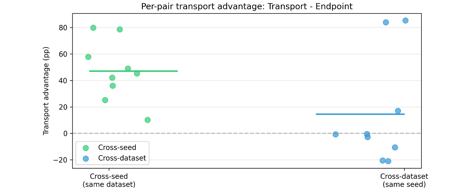
Within-run recovery. Table 18 summarizes base\(\to\)final recovery within each run. Residual-stream transport remains accurate even at 1500 steps, while FFN transport can degrade over long trajectories; Table 19 provides the per-run breakdown. We also include an additional within-run summary for Llama-3.2-1B.
| Metric | 200 steps | 1500 steps |
|---|---|---|
| Qwen2.5-1.5B residual transport | \(98.1\pm5.0\) | \(95.3\pm6.6\) |
| Qwen2.5-1.5B residual endpoint | \(38.3\pm11.8\) | \(27.9\pm6.4\) |
| Qwen2.5-1.5B FFN transport | \(96.3\pm4.0\) | \(72.6\pm25.3\) |
| Qwen2.5-1.5B FFN endpoint | \(75.7\pm17.0\) | \(30.7\pm6.7\) |
| Llama-3.2-1B residual transport | \(93.5\pm5.2\) | \(81.6\pm31.2\) |
| Llama-3.2-1B residual endpoint | \(37.8\pm9.0\) | \(20.9\pm8.0\) |
| Dataset/seed | Res. endpoint | Res. transport | FFN endpoint | FFN transport |
|---|---|---|---|---|
| code 10042 | 28.0 | 97.1 | 22.4 | 77.1 |
| code 42 | 26.4 | 99.3 | 37.6 | 92.8 |
| code 5042 | 25.7 | 99.2 | 29.7 | 97.5 |
| math 10042 | 28.6 | 91.5 | 35.8 | 68.7 |
| math 42 | 13.5 | 100.0 | 23.8 | 70.5 |
| math 5042 | 32.1 | 97.5 | 42.5 | 13.3 |
| wiki 10042 | 33.1 | 79.3 | 26.2 | 80.7 |
| wiki 42 | 27.5 | 99.1 | 28.5 | 91.0 |
| wiki 5042 | 35.9 | 95.1 | 30.3 | 61.9 |
17.1 Intervention transfer: cross-run steering vector transfer↩︎
Gauge recovery accuracy measures coordinate-level alignment, but does this translate to improved interpretability? We test whether steering vectors extracted from one independently trained model transfer effectively to another model trained from the same base.
Setup. Using the same cross-run setup, we extract sentiment steering vectors and apply them across runs. We report results for Qwen2.5-1.5B (28 layers; residual layers \(\{7,14,21\}\)) and Llama-3.2-1B (16 layers; residual layers \(\{4,8,12\}\)). Let \(T_r\) denote the transport base\(\to\)final map for run \(r\) and \(E_r\) the endpoint base\(\to\)final map (one-shot matching of \(t_0\) and \(t_T\)). Then \(G_{A\to B}=T_A^{-1}T_B\) and endpoint-via-base is \(E_A^{-1}E_B\). For each pair of models \(A\to B\), we compare:
Fresh: Steering vector extracted directly from model \(B\) (upper bound)
Transported: Vector from \(A\) transformed via transport gauge \(G_{A\to B}\)
Endpoint-mapped: Vector from \(A\) transformed via endpoint-via-base mapping \(E_A^{-1}E_B\)
We measure steering effect preservation as \(100\times\Delta_{\rm method}/\Delta_{\rm fresh}\). We treat a steering direction as detectable only if \(\Delta_{\rm fresh}>0.1\); otherwise preservation is not reported and is excluded from averages.
| Component | Transport | Endpoint | Win-rate |
|---|---|---|---|
| Qwen residual, 200 steps | 103.6 | 33.2 | 54/54 |
| Qwen residual, 1500 steps | 80.5 | 18.4 | 50/52 |
| Qwen FFN layer 14, 200 steps | 84.8 | 25.2 | 13/14 |
| Qwen FFN layer 14, 1500 steps | 38.3 | -6.2 | 12/16 |
| Llama-3.2 residual, 200 steps | 99.1 | 53.5 | 54/54 |
| Llama-3.2 residual, 1500 steps | 68.4 | 38.9 | 40/52 |
| Behavior | Gauge | Step 0 | Transport | Steering preservation |
|---|---|---|---|---|
| Sentiment | \(\Bd\) | 100.0% | 92.7% | 95.8% |
| Sentiment | \(\Sd\) | 48.2% | 27.3% | 17.2% |
| Refusal | \(\Bd\) | 100.0% | 92.6% | +150.5% |
| Refusal | \(\Sd\) | 48.2% | 25.9% | -32.2% |
Permutation-only comparison. Table 21 reports the Qwen2.5-1.5B rows used in Table 5. This comparison uses the WikiText cross-seed pair (source seed 42, target seed 5042) after 1500 fine-tuning steps. The \(B_d\) rows compose signed-permutation gauges; the \(S_d\) rows use the same permutation maps with all signs fixed to \(+1\). Preservation is averaged over residual layers \(\{7,14,21\}\) when the fresh target effect is detectable; for refusal, layer 7 is excluded because the fresh effect is below the detectability threshold.
FFN steering detectability. In the Qwen2.5-1.5B FFN steering-transfer evaluation we probe three pre-chosen layers \(\{7,14,21\}\) (for consistency with the residual-stream experiments). However, the fresh in-target FFN intervention is often negligible at layers 7 and 21, making preservation ratios ill-conditioned. We therefore treat a layer as not detectable when \(\Delta_{\rm fresh}\le 0.1\) and exclude it from preservation averages. Table 22 reports detectability rates for transparency: layer 14 is detectable in the majority of pairs, whereas layers 7 and 21 are rarely detectable.
Reporting policy for FFN steering. All FFN steering-transfer preservation numbers are reported for layer 14 only, where the fresh in-target intervention is most consistently detectable (Table 22).
Scope of steering transfer. The cross-run steering-transfer experiment evaluates sentiment steering; broader behaviors and architectures are not evaluated in this experiment. FFN gauge tracking is less stable than residual-stream tracking over long trajectories in some runs (Table 19), suggesting more robust FFN matching (or periodic re-anchoring) is required for long-horizon FFN transport.
18 Optimizer-state resumption details↩︎
The stateful-resumption run compares resumed trajectories, not endpoint losses. For AdamW, \(B_d\) transport applies signs to the first moment \(m_W\) according to each parameter’s
READ/WRITE role, while the second moment \(v_W\) is transported by the unsigned permutation because signs square out. The \(S_d\) ablation applies the correct permutation but omits signs in
\(m_W\). The main Qwen2.5-0.5B row uses float32, AdamW with learning rate \(2\times10^{-5}\), weight decay 0.01, gradient clipping at 1.0, sequence length 128, 2048 training
texts, four held-out evaluation batches, and a trainable suffix of four decoder layers (trainable_scope=last_n, last_n_layers=4). The fp32 rows are the primary tests of exact gauge covariance.
| FFN layer | 200 steps | 1500 steps |
|---|---|---|
| 7 | 3/18 | 0/18 |
| 14 | 14/18 | 16/18 |
| 21 | 3/18 | 3/18 |
| Model/opt. | Setup | Pre | \(\Bd\) | \(\Sd\) | Other variants |
|---|---|---|---|---|---|
| Qwen2.5-0.5B AdamW | fp32 \(b=1\), 30+10 | \(1.86\times10^{-12}\) | \(1.05\times10^{-12}\) | \(2.08\times10^{-2}\) | \(2.54\times10^{-3}\)–\(7.57\times10^{-2}\) |
| Qwen2.5-0.5B SGD \(\mu=0.9\) | fp32 \(b=1\), 50+10 | \(9.28\times10^{-12}\) | \(5.11\times10^{-12}\) | \(3.83\times10^{-2}\) | \(2.72\times10^{-2}\)–\(7.10\times10^{-2}\) |
| TinyLlama-1.1B AdamW | fp32 \(b=1\), 30+10 | \(5.64\times10^{-13}\) | \(3.25\times10^{-13}\) | \(3.77\times10^{-3}\) | \(1.35\times10^{-3}\)–\(1.50\times10^{-2}\) |
| Qwen2.5-0.5B AdamW | fp32 \(b=8\), 200+200 | \(1.51\times10^{-12}\) | \(5.75\times10^{-12}\) | \(3.72\times10^{-4}\) | \(3.48\times10^{-4}\)–\(4.69\times10^{-4}\) |
| Qwen2.5-0.5B AdamW | fp32 \(b=32\), 500+500 | \(5.24\times10^{-12}\) | \(5.30\times10^{-10}\) | \(3.50\times10^{-3}\) | \(3.88\times10^{-3}\)–\(7.04\times10^{-3}\) |
19 SAE and steering tool-transfer details↩︎
The TinyLlama-1.1B tool-transfer experiment isolates the sign variable with a known gauge. We train an SAE and extract CAA steering vectors on model A, apply a random \(B_d\) gauge to obtain functionally equivalent model B, recover the gauge from activations alone, and transfer the tools to B. The probe set contains 100 texts (11,134 tokens). Full \(B_d\) recovery obtains 100% joint permutation/sign accuracy. The transferred SAE has normalized reconstruction MSE 0.004, matching the recovered-gauge reference. The signed-cost \(S_d\) recovery pipeline hits the structural ceiling of Theorem 4: it recovers only the positive-sign half of the coordinates and gives SAE NMSE 1.08. Separately, steering vectors use the matched permutation with signs forced to \(+1\), isolating orientation loss; across sentiment, sycophancy, and refusal this degrades or inverts all three effects, ranging from \(-14\%\) to \(-80\%\).
| Condition | Perm/sign recovery | SAE NMSE |
|---|---|---|
| \(\Bd\) recovery (ours) | 100% / 100% | 0.004 |
| \(\Sd\) signed-cost recovery | 50% / – | 1.08 |
| Recovered-gauge reference | 100% / 100% | 0.004 |
20 Natural sign mismatch in independent training↩︎
Question: The merge experiments in §5 include gauge-scramble settings. Does sign mismatch also occur between independently trained models?
Answer: Yes, in this small-scale run. Two RMSNorm models trained from different seeds develop 50% sign mismatch, and signed alignment outperforms perm-only by 37%.
20.0.0.1 Setup.
We train two identical 4-layer Llama-style transformers (256 hidden, RMSNorm, \(\sim\)10M params) on WikiText [Merity et al., 2017] for 1000 steps, differing only in initialization seed. We then estimate the gauge relating them via activation-based Hungarian matching. This is a low-dimensional same-data example, not evidence that \(\sim 500\) probe tokens suffice for natural alignment of large LLMs; larger natural LLM alignment remains probe-hungry as in Appendix 15.2.
20.0.0.2 Sign mismatch occurs without an imposed gauge in this run.
The models exhibit 50% sign disagreement: half of matched neuron pairs learned opposite sign conventions. This is expected—RMSNorm models have \(B_d\) symmetry, and independent training runs break this symmetry differently.
20.0.0.3 Signed alignment helps.
Table 25 shows merge barrier peaks. Perm-only alignment (\(S_d\)) reduces the peak barrier by 61%, but signed alignment (\(B_d\)) achieves 75% reduction—a 37% relative improvement from accounting for signs.
20.0.0.4 Takeaway.
This small-scale natural run shows that sign mismatch can also arise between independently trained RMSNorm models.
| Alignment | Barrier peak (\(\Delta\)NLL) | Reduction |
|---|---|---|
| Unaligned | 1.68 | – |
| Perm-only (\(\Sd\)) | 0.66 | 61% |
| Signed (\(\Bd\)) | 0.42 | 75% |
20.1 Additional 0-step gauge-equivalent merge: TinyLlama-1.1B↩︎
The same gauge-scramble merge setup also applies to a smaller RMSNorm decoder, TinyLlama/TinyLlama-1.1B-Chat-v1.0, with 0 fine-tuning steps. Thus the two endpoints are exactly gauge-equivalent, and a
symmetry-respecting alignment should eliminate the peak barrier. Table 26 shows that perm-only alignment with the correct permutation but signs forced to \(+1\) does not reduce the peak
barrier relative to unaligned averaging, while signed alignment (ours; \(B_d\)) eliminates it.
| Alignment | Barrier peak (\(\Delta\)NLL) |
|---|---|
| Unaligned | 6.36 |
| Perm-only (correct permutation) | 6.47 |
| Signed (ours) | 0.00 |
20.2 Minimal example: \(S_d\)-only alignment can worsen averaging under \(B_d\)↩︎
We give a minimal example illustrating the cancellation mechanism behind “perm-only worse than unaligned” when the true symmetry group includes sign flips.
Proposition 17 (Permutation-only alignment can increase midpoint loss under \(B_d\)). There exist two \(B_d\)-gauge-equivalent parameterizations of the same function such that averaging after a permutation-only (\(S_d\)) alignment step yields strictly higher midpoint loss than unaligned averaging.
20.2.0.1 Proof.
Consider the two-layer linear network \(f_\theta(x)=xAB\) with \(A=B=I_2\) and squared-error loss to targets \(y=x\) under isotropic inputs with \(\mathbb{E}\left\lVert x \right\rVert_2^2<\infty\). Let \[P=\begin{bmatrix}0&1\\1&0\end{bmatrix}, \qquad S=\operatorname{diag}(-1,1), \qquad G:=PS=\begin{bmatrix}0&1\\-1&0\end{bmatrix}\in B_d,\] so \(GG^\top=I_2\) and \(G^\top=-G\). Define gauge-transformed parameters by \(A^G=AG\) and \(B^G=G^\top B\), so \(f_{\theta^G}(x)=xA^GB^G=x\) and \(\theta\) and \(\theta^G\) are gauge-equivalent.
For unaligned averaging, midpoint parameters are \(A_{1/2}=\frac{1}{2}(I_2+G)\) and \(B_{1/2}=\frac{1}{2}(I_2+G^\top)\), giving \(A_{1/2}B_{1/2}=\frac{1}{4}(I_2+G+G^\top+GG^\top)=\frac{1}{2}I_2\). Thus \(f_{1/2}(x)=\frac{1}{2}x\) and expected midpoint loss is \(\frac{1}{4}\mathbb{E}\left\lVert x \right\rVert_2^2\).
For \(S_d\)-only alignment, a permutation-only alignment can remove the permutation component \(P\) but cannot apply the required sign flip. Composing with \(P\) yields sign-only mismatch \(GP=\operatorname{diag}(1,-1)\). Averaging \(\theta\) with \(\theta^{GP}\) gives \(A_{1/2}=\frac{1}{2}(I_2+GP)=\operatorname{diag}(1,0)\) and \(B_{1/2}=\operatorname{diag}(1,0)\), so \(f_{1/2}(x)=(x_1,0)\). The expected midpoint loss is \(\mathbb{E}[x_2^2]=\frac{1}{2}\mathbb{E}\left\lVert x \right\rVert_2^2\), strictly larger than \(\frac{1}{4}\mathbb{E}\left\lVert x \right\rVert_2^2\).
21 Extended related work↩︎
21.0.0.1 Permutation symmetries and mode connectivity.
Hidden-unit permutations have long been known to create equivalent parameterizations and connected loss landscapes [Brea et al., 2019, Freeman and Bruna, 2017, Draxler et al., 2018, Garipov et al., 2018, Tatro et al., 2020, Entezari et al., 2022]. Git Re-Basin turns this into an alignment procedure over \(S_d\) [Ainsworth et al., 2023]. Our contribution is the architecture-dependent residual-stream group for transformers: per-index \(S_d\) for LayerNorm and \(B_d\) for RMSNorm, together with the ceiling theorem showing why the missing sign component is structurally unrecoverable by signed-correlation matching.
21.0.0.2 Continuous and rotation-based methods.
SliceGPT, QuaRot, generalized linear mode connectivity, and rotation-aware fusion exploit broader \(O(d)\) freedom after reparameterization [Ashkboos et al., 2024a,b, Theus et al., 2025, Zhang et al., 2025]. These methods solve different alignment problems. They can be stronger for coordinate-indifferent compression or fusion; they are not coordinate-preserving transports of sparse objects in the native \(\gamma\)-explicit model. Theorem 2 gives the interface: extract the \(B_d\) component when coordinates matter, use the residual dense rotation when they do not.
21.0.0.3 Model merging and interpretability.
Merging methods include weight matching, model soups, task arithmetic, TIES, ZipIt!, and optimal-transport fusion [Ainsworth et al., 2023, Wortsman et al., 2022, Ilharco et al., 2023, Yadav et al., 2023, Stoica et al., 2024, Singh and Jaggi, 2020, Imfeld et al., 2024, Verma and Elbayad, 2024, Yang et al., 2024b]. Our merge results are not a universal merging recipe; they identify a necessary discrete correction for RMSNorm coordinate-preserving alignment.
In interpretability, invariant representation metrics remain valid without gauge fixing [Raghu et al., 2017, Morcos et al., 2018, Kornblith et al., 2019]; direction and subspace analyses are similarly invariant within a fixed chart [Elhage et al., 2023]. Our audit targets the complementary class of analyses that output indices. SAE dictionary studies identify feature indices with semantic labels [Bricken et al., 2023, Gao et al., 2025]: Bricken et al. [2023] report “feature A/1/2357” as a base64-input detector and characterize hundreds of similarly-indexed features with concept labels. Knowledge-neuron pipelines locate factual associations at specific MLP hidden units: Dai et al. [2022] identify \(w^{(9)}_{2141}\) and \(w^{(10)}_{1122}\) as carrying the Ireland–Dublin association, and report similar coordinate triples for other facts. Direction-level steering work [Rimsky et al., 2024, Arditi et al., 2024] makes single-model claims that are gauge-invariant in isolation but require a coordinate map to be compared or transferred across runs or related models, which is exactly what Proposition 3 characterizes.
These examples have different native gauges: BERT-style FFN neuron claims are relative to hidden-unit permutations, while residual-stream artifacts in RMSNorm Llama/Qwen/TinyLlama charts live on a \(B_d\) orbit of size \(2^d d!\). The dependence is not hypothetical. Paulo and Belrose [2026] report only \(\sim30\%\) SAE feature overlap across training seeds on Llama 3 8B; our TinyLlama transfer experiment shows that on a single model, ignoring the residual \(B_d\) component drives SAE reconstruction NMSE from 0.004 to 1.08–a \(270\times\) degradation under an exact symmetry of the model. Other sources of cross-seed disagreement also exist (optimization noise, data order, feature splitting), but the residual gauge is a formally identifiable component, and the audit specifies the controls that isolate it.
22 Detailed limitations and broader impacts↩︎
22.0.0.1 Detailed limitations.
First, our transport experiments measure recovery along real Qwen2.5-1.5B fine-tuning trajectories against coordinate correspondences induced by randomly sampled \(B_d\) gauges applied at step 0 and recorded as ground truth; the complementary regime–coordinate alignment between independently specified parameterizations from function-level information alone–is shown by Proposition 5 to admit no canonical answer, so its absence here reflects the structure of the symmetry rather than an algorithmic gap. Second, transport involves stride and probe-distribution choices, and FFN transport is less stable over long horizons than residual-stream transport. Third, exact repeated \(\gamma\) values create global stabilizer intersections, while near-repeats reduce assignment margins; activation matching then selects a probe-dependent \(B_d\) representative. Fourth, our audits target the subset of interpretability and adaptation workflows that output coordinate names. Coordinate-level claims complement invariant analyses, and coordinate-level claims on RMSNorm models require gauge specification.
22.0.0.2 Broader impacts.
Gauge-correct transport can improve reproducibility and checkpoint-editing audits, but can also lower the cost of transferring behavioral interventions, including undesirable steering directions, between related checkpoints. We therefore present it as an audit and verification tool, and emphasize gauge-invariant reporting when coordinate identity is unnecessary.