Attend, Transform, or Silence: Operator-Level Visual Skipping for Efficient Multimodal LLM Inference
June 30, 2026
Abstract
Multimodal large language models (MLLMs) increasingly process long visual-token sequences, increasing the overall inference computation. Existing acceleration methods usually remove visual tokens or skip visual-token updates in entire layers, but these coarse strategies may discard fine-grained evidence or suppress useful operators together with redundant ones. In this paper, we study visual-token computation from an answer-observable perspective and find that late visual-token updates can remain large while having little effect on answer-token representations. Motivated by this answer-silent redundancy, we decompose each Transformer layer into attention and FFN operators and show that useful visual computation is often operator-dominant and layer-dependent. We propose an operator-level visual-token skipping framework that preserves the full visual-token sequence while selectively bypassing redundant attention, FFN, or both. Experiments across three MLLM architectures and 10 VQA benchmarks show that our method achieves strong efficiency-accuracy trade-offs, reducing 33.7% TFLOPs on Qwen3-VL while retaining 99.5% of the vanilla model performance.1
1 Introduction↩︎
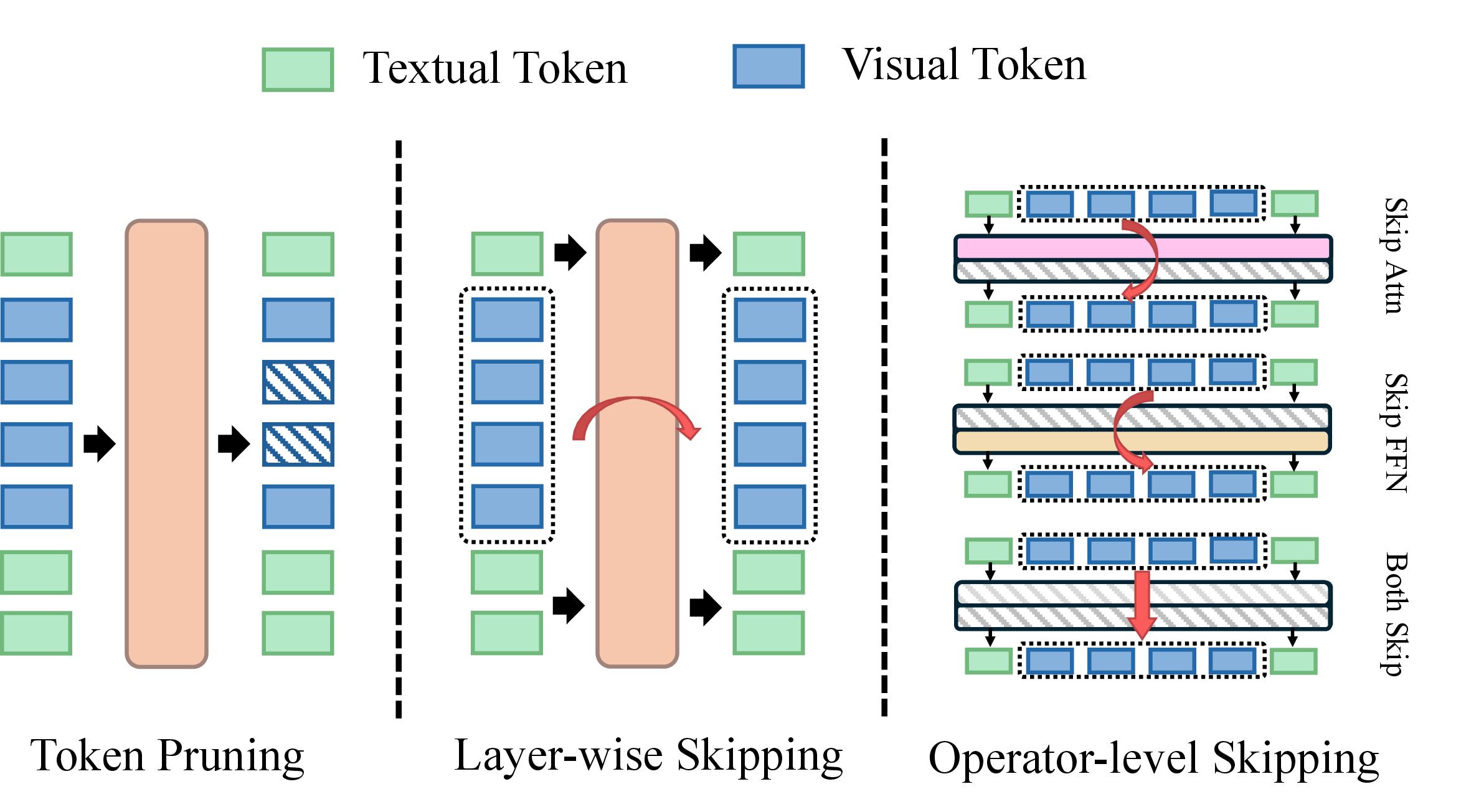
Multimodal large language models (MLLMs) [1]–[5] have become a central paradigm for visual understanding, visual reasoning, and visual question answering. A typical MLLM encodes an image into visual tokens, projects them into the embedding space of a large language model (LLM), and concatenates them with text tokens for autoregressive generation [1], [4], [5]. To preserve fine-grained visual evidence, recent MLLMs increasingly adopt high-resolution inputs, image tiling, or dense visual encoders, expanding the visual sequence from hundreds to thousands of tokens [3]–[6]. While this improves perceptual coverage, it also makes the prefill stage expensive, as the LLM backbone must process all visual and textual tokens simultaneously through self-attention and feed-forward transformations [7]. A growing body of work therefore accelerates MLLMs by reducing visual computation, either by pruning, selecting, or merging visual tokens [8]–[11], or by skipping visual-token updates in selected Transformer layers [12]–[14]. These methods show that not all visual computation is equally necessary, but they rely on coarse notions of redundancy. Token-level methods may permanently discard fine-grained evidence, layer-level skipping removes attention and FFN computation together, and V-Skip [14] assumes a fixed preference for preserving FFN while skipping visual attention. Such fixed granularities cannot decide whether attention, FFN, or both are redundant at each layer, and may suppress useful computation when only part of a layer is redundant.
In this paper, we revisit visual redundancy in MLLMs by examining how visual tokens evolve inside the LLM backbone. We begin with a counterintuitive observation, in late layers, visual-token hidden states can still change substantially, even when these changes have little influence on the final answer. This indicates that update magnitude alone is not a reliable measure of useful visual computation. To distinguish representational movement from computation that actually affects answer generation, we introduce a set of answer-observable diagnostics, which measure how visual-token updates propagate to answer-token hidden states. Across multiple MLLM architectures and VQA benchmarks, we consistently find that late visual tokens often undergo large hidden-state updates while exhibiting small answer-observable effects. These updates are therefore not inactive, but answer-silent, they consume computation while contributing little to the representations that determine the generated response.
This observation suggests that visual redundancy is not merely a property of individual tokens, nor is it always aligned with entire Transformer layers. Instead, redundancy may emerge at a finer operator level within each layer. This view is supported by recent analyses of LVLM backbones [15], which reveal a functional decoupling between attention and FFN operators, attention primarily reconfigures information within a relatively preserved representation subspace, whereas FFNs expand the representation subspace and drive semantic transformation. If these two operators serve different representational roles, their importance for visual tokens should not be assumed to be coupled in every MLLM layer. Some layers may require attention to route visual evidence toward the question, some may rely more on FFN transformations to refine visual semantics, and others may contribute little through either operator.
Motivated by this observation, we decompose each Transformer layer into its attention and FFN operators and ask a finer question: which operator is actually necessary for visual-token computation in each layer? By separately measuring the answer-observable contribution of attention and FFN, we find strong layer-wise heterogeneity, some layers are attention-dominant, some are FFN-dominant, and others show little answer-observable contribution. Based on this observation, we propose an operator-level visual-token skipping framework that preserves the full visual-token sequence while bypassing redundant visual computation. This design avoids the irreversible evidence loss of token pruning and releases visual skipping from the static assumption that either attention or FFN is always the important operator. Experiments across multiple MLLM architectures and 10 visual question answering benchmarks show that our framework substantially reduces visual computation during inference while maintaining answer quality, achieving up to 33.7% visual-computation reduction with only 0.5% average performance change. Beyond efficiency, our analysis suggests that useful visual computation in MLLMs is operator-dependent rather than block-aligned, and that efficient inference should be designed around answer-observable computation rather than raw update magnitude or fixed architectural boundaries.
Our contributions are summarized as follows:
We identify answer-silent visual-token updates in late MLLM layers and introduce answer-observable diagnostics to measure whether visual computation actually propagates to answer-token representations.
We reveal that useful visual computation is operator-dominant and layer-dependent by decomposing each Transformer layer into attention and FFN operators, exposing visual redundancy beyond token- and layer-level views.
We propose an operator-level visual-token skipping framework that preserves the full visual-token sequence while bypassing redundant visual computation, saving up to 33.7% visual computation while retaining 99.5% model performance across Qwen3VL and 10 VQA benchmarks.
2 Answer-Silent Visual Updates in MLLM↩︎
We first examine when visual-token information is effectively used by the textual stream during the prefill stage. In mainstream decoder-only MLLMs [1], [4], [5], visual tokens are placed before the textual prompt and processed under causal masking. As a result, the last prompt token is the first position that can integrate both the visual prefix and the textual question. Its hidden state, which we refer to as the final prompt-token hidden state, is directly projected by the language-modeling head to produce the next-token logits. This motivates the following diagnostic question:
Let \(H_v^l \in \mathbf{R}^{N_v \times d}\) denote the visual-token hidden states at layer \(l\), where \(N_v\) is the number of visual tokens and \(d\) is the hidden dimension. We first quantify the magnitude of visual-token state changes between consecutive layers: \[{!}{\displaystyle \Delta V_l = H_v^{l+1} - H_v^l,\quad \mathrm{VUM}_l = \frac{|\Delta V_l|_F}{\max_j |\Delta V_j|_F + \epsilon}. } \label{eq:vum}\tag{1}\] We refer to this normalized quantity as visual update magnitude (VUM), where larger values indicate stronger visual-state changing.
To measure whether such changing is observable from the answer side, we estimate its first-order influence on the final prompt-token hidden state. Let \(h_{\mathrm{last}}\) denote the final prompt-token hidden state during prefill, and let \[J_l = \frac{\partial h_{\mathrm{last}}}{\partial H_v^{l+1}}\] be the Jacobian that maps perturbations of visual-token states at layer \(l+1\) to changes in \(h_{\mathrm{last}}\). We define \[\delta h_l = J_l[\Delta V_l], \qquad \mathrm{AOI}_l = |\delta h_l|_2 . \label{eq:aoi}\tag{2}\] and we call \(\mathrm{AOI}_l\) answer-observable influence (AOI), where \(J_l[\Delta V_l]\) is the Jacobian-vector product estimating how the visual update at layer \(l\) changes the final prompt-token hidden state.
Finally, we normalize AOI by the size of the visual update: \[{!}{\displaystyle \mathrm{AOE}_l = \frac{\mathrm{AOI}_l}{\|\Delta V_l\|_F + \epsilon}\; \widetilde{\mathrm{AOE}}_l = \frac{\mathrm{AOE}_l}{\max_j \mathrm{AOE}_j + \epsilon}. } \label{eq:aoe}\tag{3}\] We refer to this quantity as answer-observable efficiency (AOE). In summary, VUM measures the magnitude of visual-token changes, AOI measures how much these changes reach the final prompt-token hidden state, and AOE measures the answer-observable influence per unit of visual-token update.
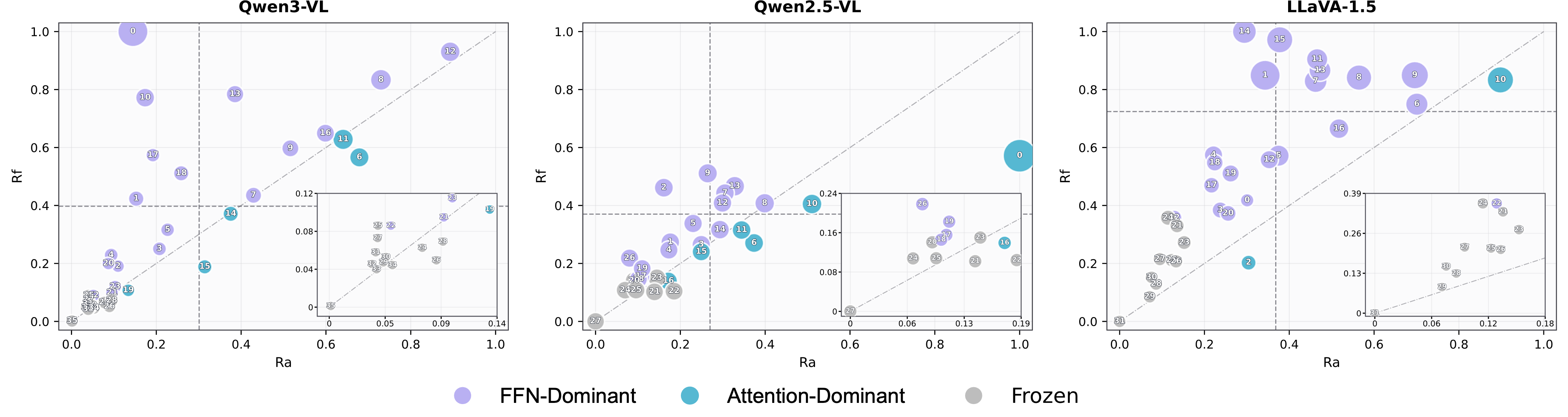
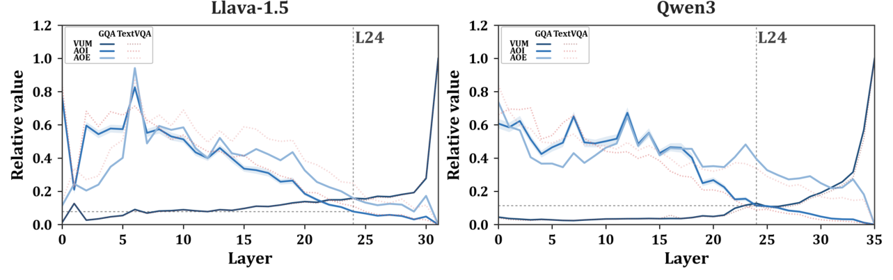
Figure 2 shows the layer-wise behavior of VUM, AOI, and AOE on GQA and TextVQA for LLaVA-1.5 and Qwen3-VL. The curves reveal a consistent late-layer decoupling: visual-token states continue to change substantially, while their answer-observable influence decreases. In LLaVA-1.5, VUM rises sharply after layer 24, whereas both AOI and AOE continue to decline. Qwen3-VL exhibits the same pattern around its decoupling onset layer. Thus, raw update magnitude systematically overestimates the usefulness of late visual computation.
This observation suggests a direct intervention. If late visual-token updates are weakly coupled to answer generation, freezing visual-token states after the decoupling onset layer should have limited impact on task performance. We therefore freeze visual-token hidden states after layer 24 while keeping all text-token computation unchanged. Concretely, for layers \(l > 24\), we reuse the visual states from layer 24 and allow textual tokens to continue attending to these fixed visual representations. This removes late visual-state changes while preserving the visual evidence accessible to textual tokens.
| Model | Method | GQA | POPE | TextVQA | SQA |
|---|---|---|---|---|---|
| Full | 61.9 | 85.9 | 58.2 | 69.5 | |
| Frozen visual | 61.1\(_{\textcolor{green}{\downarrow0.8}}\) | 86.4\(_{\textcolor{red}{\uparrow0.5}}\) | 57.2\(_{\textcolor{green}{\downarrow1.0}}\) | 69.6\(_{\textcolor{red}{\uparrow0.1}}\) | |
| Full | 61.6 | 89.1 | 80.0 | 94.4 | |
| Frozen visual | 61.3\(_{\textcolor{green}{\downarrow0.3}}\) | 88.9\(_{\textcolor{green}{\downarrow0.2}}\) | 80.1\(_{\textcolor{red}{\uparrow0.1}}\) | 94.4 |
As shown in Table 1, freezing late visual-token states causes only marginal degradation on 4 benchmarks across the two MLLM architectures. This result indicates that repeatedly updating visual-token states is often not the computation that determines next-token prediction. The model can still access visual evidence through the textual stream, while the continued changes of late visual-token states become increasingly answer-silent.
This finding motivates a finer-grained analysis of where useful visual computation resides within each Transformer block. We therefore move beyond the block-level view and decompose each layer into its attention and FFN operators, analyzing which operator dominates answer-observable visual computation at different depths.
3 Methodology↩︎
3.1 Operator Risk Analysis↩︎
We first describe how to identify the layer-wise operator structure of the visual branch without retraining the model or using human-annotated answers. Given a decoder-only MLLM, let the hidden states at layer \(l\) be \[H^l = [H_{\mathcal{V}}^l; H_{\mathcal{T}}^l].\] where \(H_{\mathcal{V}}^l \in \mathrm{R}^{N_v \times d}\) denotes the visual-token hidden states and \(H_{\mathcal{T}}^l\) denotes the textual hidden states, including the system prompt, question tokens, and possible answer-prefix tokens. We decompose the visual branch of a Transformer block into two residual updates: \[\begin{align} \bar{H}_{\mathcal{V}}^{l} &= H_{\mathcal{V}}^{l} + \big[A^{l}(H^{l})\big]_{\mathcal{V}}, \\ H_{\mathcal{V}}^{l+1} &= \bar{H}_{\mathcal{V}}^{l} + \big[F^{l}(\bar{H}^{l})\big]_{\mathcal{V}} . \end{align} \label{eq:operator95decomposition}\tag{4}\] where \(A^{l}\) is the self-attention update and \(F^{l}\) is the FFN update at layer \(l\). The subscript \(\mathcal{V}\) denotes the visual-token rows. This decomposition allows us to ask a more fine-grained question than whether an entire layer can be skipped:
For an input sample \(x\), the full model produces a reference next-token distribution from the final prompt-token hidden state after prefill: \[p_0(\cdot|x)=\mathrm{softmax}(z_0(x)).\] This reference distribution is obtained from the model itself and does not require ground-truth labels. We estimate layer-wise operator risks on a small calibration set \(\mathcal{D}\) sampled from multiple benchmarks, using these samples only to probe how the output distribution changes under counterfactual visual-operator interventions. \[\begin{align} &\frac{1}{|\mathcal{D}|} \sum_{x\in\mathcal{D}} D_{\mathrm{KL}}\!\left( p_0(\cdot|x)\Vert p_{s}^{(l)}(\cdot|x) \right), \\ &\quad s\in\{\mathcal{A},\mathcal{F},\mathcal{AF}\}. \end{align}\]
Here, \(\mathcal{R}{\mathcal{A}}(l)\), \(\mathcal{R}{\mathcal{F}}(l)\), and \(\mathcal{R}_{\mathcal{AF}}(l)\) measure the output risk of removing visual attention, removing visual FFN, and freezing the visual branch at layer \(l\), respectively.
\[\log \frac{\mathcal{R}{\mathcal{A}}(l)+\epsilon}{\mathcal{R}{\mathcal{F}}(l)+\epsilon}.\] A positive \(\Gamma_l\) indicates an attention-dominant layer, while a negative \(\Gamma_l\) indicates an FFN-dominant layer. Layers with uniformly small risks, especially small \(\mathcal{R}_{\mathcal{AF}}(l)\), are treated as frozen layers.
3.2 Operator-Aware Skipping↩︎
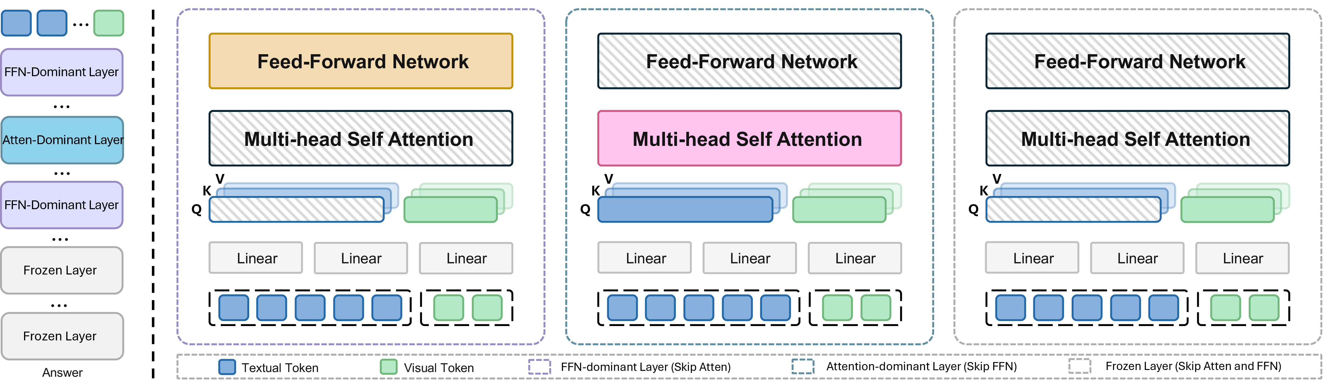
We convert the layer-wise risk profile into an inference-time skipping policy through two steps, budgeted layer selection and policy assignment. Given a compute budget \(B\), we rank layers by \(\mathcal{R}{\mathcal{A}}(l)+\mathcal{R}{\mathcal{F}}(l)\) and select the \(B\) lowest-risk layers for simplification. These are layers where removing either visual attention or visual FFN individually induces only a small output shift.
For each selected layer, we assign the least risky visual-branch policy. If \(\mathcal{R}{\mathcal{A}}(l) < \mathcal{R}{\mathcal{F}}(l)\), we apply FFN-only, skipping visual attention while preserving visual FFN. If \(\mathcal{R}{\mathcal{F}}(l) < \mathcal{R}{\mathcal{A}}(l)\), we apply Attention-only, preserving visual attention while skipping visual FFN. If \(\mathcal{R}{\mathcal{AF}}(l)\) is sufficiently small, we apply the more aggressive Freeze-update policy, skipping both visual operators and directly propagating \(H{\mathcal{V}}^l\) to the next layer.
Unlike token pruning, our method preserves the full visual-token sequence and avoids irreversible evidence removal. Unlike layer-level skipping, it does not treat attention and FFN as an inseparable block, but preserves the dominant visual operator while bypassing redundant visual-branch computation.
| Model | Method | TFLOPs | GQA | TextVQA | MME | MMB | MMMU | POPE | SQA | AI2D | OCRB | VizWiz | Avg. Ret. |
|---|---|---|---|---|---|---|---|---|---|---|---|---|---|
| LLaVA-1.5-7B | Vanilla | 100% | 61.94 | 58.21 | 1866.15 | 64.18 | 36.11 | 85.94 | 69.46 | 55.18 | 31.50 | 54.09 | 100.0 |
| VTW (K=16) | 55% | 54.77 | 52.17 | 1852.02 | 63.92 | 35.67 | 86.89 | 69.71 | 55.38 | 5.20 | 49.68 | 88.6 | |
| ShortV (N=20) | 55% | 60.49 | 53.63 | 1831.26 | 64.60 | 35.67 | 86.19 | 68.27 | 54.24 | 28.10 | 49.65 | 96.5 | |
| VSkip (N=20) | 76% | 60.77 | 57.21 | 1766.56 | 64.69 | 35.56 | 87.33 | 69.16 | 55.12 | 30.80 | 53.95 | 98.9 | |
| VSkip+ (N=20) | 76% | 61.63 | 57.21 | 1840.62 | 64.60 | 36.44 | 87.26 | 69.26 | 55.12 | 30.50 | 54.16 | 99.6 | |
| V2Drop | 66% | 60.51 | 55.92 | 1838.27 | 64.15 | 31.67 | 86.82 | 69.12 | 54.37 | 29.70 | 52.56 | 97.0 | |
| APET | 66% | 60.45 | 56.36 | 1841.29 | 64.09 | 36.11 | 86.82 | 68.93 | 55.54 | 29.90 | 53.23 | 98.7 | |
| Ours (N=20) | 66% | 60.84 | 56.40 | 1841.68 | 64.52 | 35.67 | 87.26 | 69.16 | 55.18 | 30.20 | 52.75 | 98.8 | |
| Qwen2.5-VL-7B | Vanilla | 100% | 60.40 | 77.77 | 2515.82 | 83.25 | 50.00 | 87.62 | 87.51 | 82.42 | 84.10 | 70.81 | 100.0 |
| VTW (K=16) | 50% | 46.01 | 65.43 | 1659.20 | 68.21 | 43.56 | 70.60 | 80.32 | 63.12 | 42.39 | 52.86 | 76.9 | |
| ShortV (N=20) | 50% | 49.47 | 71.93 | 1772.94 | 72.25 | 41.89 | 58.91 | 78.38 | 65.06 | 45.50 | 36.36 | 75.7 | |
| VSkip (N=16) | 67% | 57.26 | 63.58 | 2039.69 | 80.15 | 47.00 | 84.38 | 85.72 | 78.04 | 69.40 | 63.85 | 91.0 | |
| V2Drop | 55% | 58.87 | 72.26 | 2253.59 | 80.29 | 49.89 | 87.34 | 87.06 | 81.54 | 56.40 | 68.68 | 93.8 | |
| APET | 55% | 59.38 | 70.90 | 2263.83 | 81.70 | 50.11 | 86.70 | 87.51 | 81.54 | 60.00 | 69.02 | 94.5 | |
| Ours (N=20) | 55% | 59.29 | 72.02 | 2263.38 | 80.67 | 46.89 | 87.32 | 85.52 | 79.95 | 76.90 | 65.48 | 95.0 | |
| Qwen3-VL-8B | Vanilla | 100% | 61.60 | 80.07 | 2390.38 | 84.79 | 51.33 | 89.13 | 94.40 | 83.78 | 82.80 | 69.37 | 100.0 |
| VTW (K=16) | 58% | 43.72 | 51.16 | 1808.02 | 67.53 | 47.33 | 73.88 | 81.11 | 69.88 | 37.00 | 54.81 | 75.8 | |
| ShortV (N=20) | 58% | 60.59 | 76.08 | 2263.21 | 81.62 | 52.22 | 88.97 | 92.61 | 81.77 | 73.90 | 69.61 | 97.1 | |
| VSkip (N=20) | 76% | 60.67 | 75.98 | 2226.98 | 81.87 | 51.33 | 89.16 | 92.46 | 80.60 | 72.20 | 68.49 | 96.3 | |
| V2Drop | 66% | 60.06 | 76.44 | 2290.27 | 82.56 | 52.44 | 88.34 | 91.72 | 81.64 | 63.80 | 69.78 | 96.0 | |
| APET | 66% | 60.96 | 78.36 | 2332.50 | 82.47 | 52.53 | 88.54 | 92.56 | 82.16 | 75.80 | 68.82 | 98.0 | |
| Ours (N=20) | 66% | 60.70 | 78.45 | 2336.01 | 83.08 | 52.89 | 89.43 | 94.35 | 82.55 | 80.40 | 71.70 | 99.5 |
| Budget | GQA | TextVQA | MME | MMB | MMMU | POPE | SQA | AI2D | OCRB | VizWiz | Avg. Ret. |
|---|---|---|---|---|---|---|---|---|---|---|---|
| 0 | 61.94 | 58.21 | 1866.15 | 64.18 | 36.11 | 85.94 | 69.46 | 55.18 | 31.50 | 54.09 | 100.0 |
| 8 | 61.14 | 57.18 | 1878.10 | 64.18 | 35.67 | 86.43 | 69.61 | 55.51 | 31.40 | 53.23 | 99.6 |
| 20 | 60.84 | 56.40 | 1841.68 | 64.52 | 35.67 | 87.26 | 69.16 | 55.18 | 30.20 | 52.75 | 98.8 |
| 32 | 57.89 | 53.80 | 1728.08 | 62.03 | 35.67 | 85.01 | 69.21 | 52.46 | 25.10 | 52.76 | 94.5 |
| 0 | 60.40 | 77.77 | 2515.82 | 83.25 | 50.00 | 87.62 | 87.51 | 82.42 | 84.10 | 70.81 | 100.0 |
| 8 | 59.85 | 76.62 | 2346.15 | 82.56 | 49.11 | 87.29 | 87.41 | 82.58 | 81.80 | 68.25 | 98.2 |
| 20 | 59.29 | 72.02 | 2263.38 | 80.67 | 46.89 | 87.32 | 85.52 | 79.95 | 76.90 | 65.48 | 95.0 |
| 28 | 57.27 | 54.75 | 1884.70 | 69.07 | 39.33 | 86.29 | 77.94 | 62.08 | 42.30 | 54.81 | 79.2 |
| 0 | 61.60 | 80.07 | 2390.38 | 84.79 | 51.33 | 89.13 | 94.40 | 83.78 | 82.80 | 69.37 | 100.0 |
| 12 | 60.98 | 79.93 | 2352.81 | 84.62 | 52.44 | 88.83 | 94.70 | 83.65 | 81.90 | 70.78 | 100.0 |
| 20 | 60.70 | 78.45 | 2336.01 | 83.08 | 52.89 | 89.43 | 94.35 | 82.55 | 80.40 | 71.70 | 99.5 |
| 28 | 59.97 | 75.58 | 2158.87 | 80.93 | 51.00 | 88.42 | 85.72 | 76.39 | 71.20 | 66.86 | 94.0 |
| 36 | 58.51 | 69.91 | 1707.86 | 75.34 | 48.22 | 87.42 | 81.85 | 72.38 | 63.80 | 63.77 | 87.7 |
3.3 Complexity Analysis↩︎
Let \(N_v\) be the number of visual tokens, \(d\) the hidden dimension, and \(d_{\mathrm{ff}}\) the FFN intermediate dimension. Since our method modifies only visual rows and keeps text-token computation unchanged, the computational reduction comes from skipping visual-row attention, visual-row FFN, or both.
\[\begin{align} \Delta \mathcal{C}_{\mathcal{A}} &= \Theta\left(N_v d^2 + M_{\mathcal{V}} d\right), \\ \Delta \mathcal{C}_{\mathcal{F}} &= \Theta\left(\kappa N_v d d_{\mathrm{ff}}\right). \end{align}\] where \(\kappa=3\) for gated FFNs used in LLaMA- and Qwen-style backbones, and \(\kappa=2\) for standard two-layer FFNs. \[\begin{align} \Delta \mathcal{C}_{\mathrm{skip}} &= \sum_{l\in \mathcal{L}_{\mathrm{FFN}}} \Delta \mathcal{C}_{\mathcal{A}}^{(l)} \\ &\quad + \sum_{l\in \mathcal{L}_{\mathrm{Attn}}} \Delta \mathcal{C}_{\mathcal{F}}^{(l)} \\ &\quad + \sum_{l\in \mathcal{L}_{\mathrm{Freeze}}} \left( \Delta \mathcal{C}_{\mathcal{A}}^{(l)} + \Delta \mathcal{C}_{\mathcal{F}}^{(l)} \right). \end{align}\] Here, FFN-only skips visual attention, Attention-only skips visual FFN, and Freeze-update skips both operators. In practice, wall-clock speedup also depends on kernel implementation, memory movement, and hardware utilization; therefore, we report both theoretical FLOPs and measured first-token latency.
4 Experiments↩︎
4.1 Experimental Setup↩︎
4.1.0.1 Models.
We evaluate our method on three representative open-source MLLMs, LLaVA-1.5-7B [1], Qwen2.5-VL-7B [4], and Qwen3-VL-8B [5]. LLaVA-1.5-7B uses a fixed-resolution visual encoder and represents each image
with 576 visual tokens, while Qwen2.5-VL-7B and Qwen3-VL-8B adopt more recent Qwen-VL architectures with stronger visual encoders and dynamic-resolution image processing. This evaluation tests whether operator-level visual redundancy generalizes across
different MLLM designs. All evaluations are conducted with lmms-eval under the official benchmark protocols.
4.1.0.2 Benchmarks.
We evaluate on 10 multimodal benchmarks covering general VQA, text-rich understanding, hallucination sensitivity, multimodal reasoning, and scientific QA, GQA [16], TextVQA [17], MME [18], MMBench [19], MMMU [20], POPE [21], ScienceQA [22], AI2D [23], OCRBench [24], and VizWiz [25].
4.1.0.3 Baselines.
We compare with training-free acceleration baselines including layer-wise visual skipping methods VTW [13], ShortV [12], and V-Skip [14], as well as token-reduction methods V2Drop [26] and APET [27]. Unlike these coarse-grained baselines, our method preserves all visual tokens and selectively skips attention, FFN, or both according to layer-wise operator dominance.
4.1.0.4 Implementation details.
For each model, we estimate layer-wise visual operator risks using a small calibration set, sampling \(7\) examples from each of GQA, POPE, TextVQA, MME, MMMU, and ScienceQA. These examples are used only for estimating \(\mathcal{R}{\mathcal{A}}(l)\), \(\mathcal{R}{\mathcal{F}}(l)\), and \(\mathcal{R}_{\mathcal{AF}}(l)\). Based on the risks, each selected layer is assigned one of three policies, Attention-only, FFN-only, or Freeze-update. The resulting layer-wise policy is fixed for all samples of the same model. We report relative FLOPs ratio, and first-token latency measured on NVIDIA RTX A800 GPUs.
4.2 Main Results↩︎
Table 2 compares our method with representative layer-wise skipping and token-pruning baselines across three MLLM architectures and ten benchmarks. Our method achieves a strong accuracy–efficiency trade-off by preserving the full visual-token sequence while selectively skipping redundant operators, leading to the highest average performance retention across the evaluated backbones.
This robustness comes from keeping the dominant visual operator in each selected layer, which helps preserve fine-grained and text-rich evidence while removing answer-silent computation. Following the V-Skip paper, VSkip+ uses dataset-specific optimal settings, whereas the other methods use one configuration for all benchmarks on each model. Our single per-model policy remains competitive or superior under this comparison setting.
4.3 Efficiency Comparison on TextVQA↩︎
We further compare efficiency on TextVQA against ShortV, a competitive layer-wise visual-computation baseline. As shown in Table 4, ShortV reduces more FLOPs but causes larger accuracy degradation, whereas our method achieves comparable prefill efficiency and first-token latency while retaining stronger answer quality. This shows that operator-level skipping provides a better accuracy–efficiency balance than freezing full visual-token updates.
| Model | FLOPs | Prefill | Latency | Avg. |
|---|---|---|---|---|
| LLaVA-1.5-7B | 9.057 T | 59.1 ms | 120.4 ms | 100.0 |
| ShortV | 5.039 T | 45.0 ms | 108.2 ms | 96.5 |
| Ours | 6.475 T | 49.3 ms | 110.4 ms | 98.8 |
| Qwen3-VL-8B | 11.38 T | 95.7 ms | 465.1 ms | 100.0 |
| ShortV | 5.79 T | 45.8 ms | 310.6 ms | 97.1 |
| Ours | 7.23 T | 52.9 ms | 344.8 ms | 99.5 |
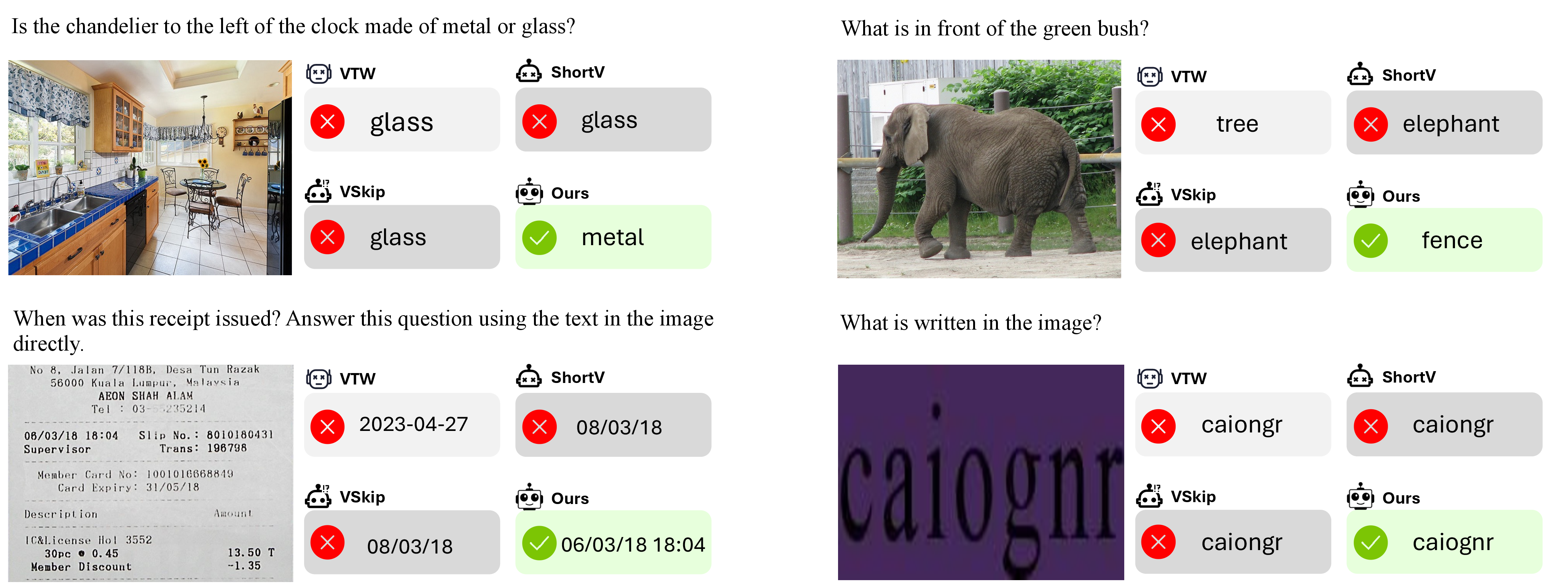
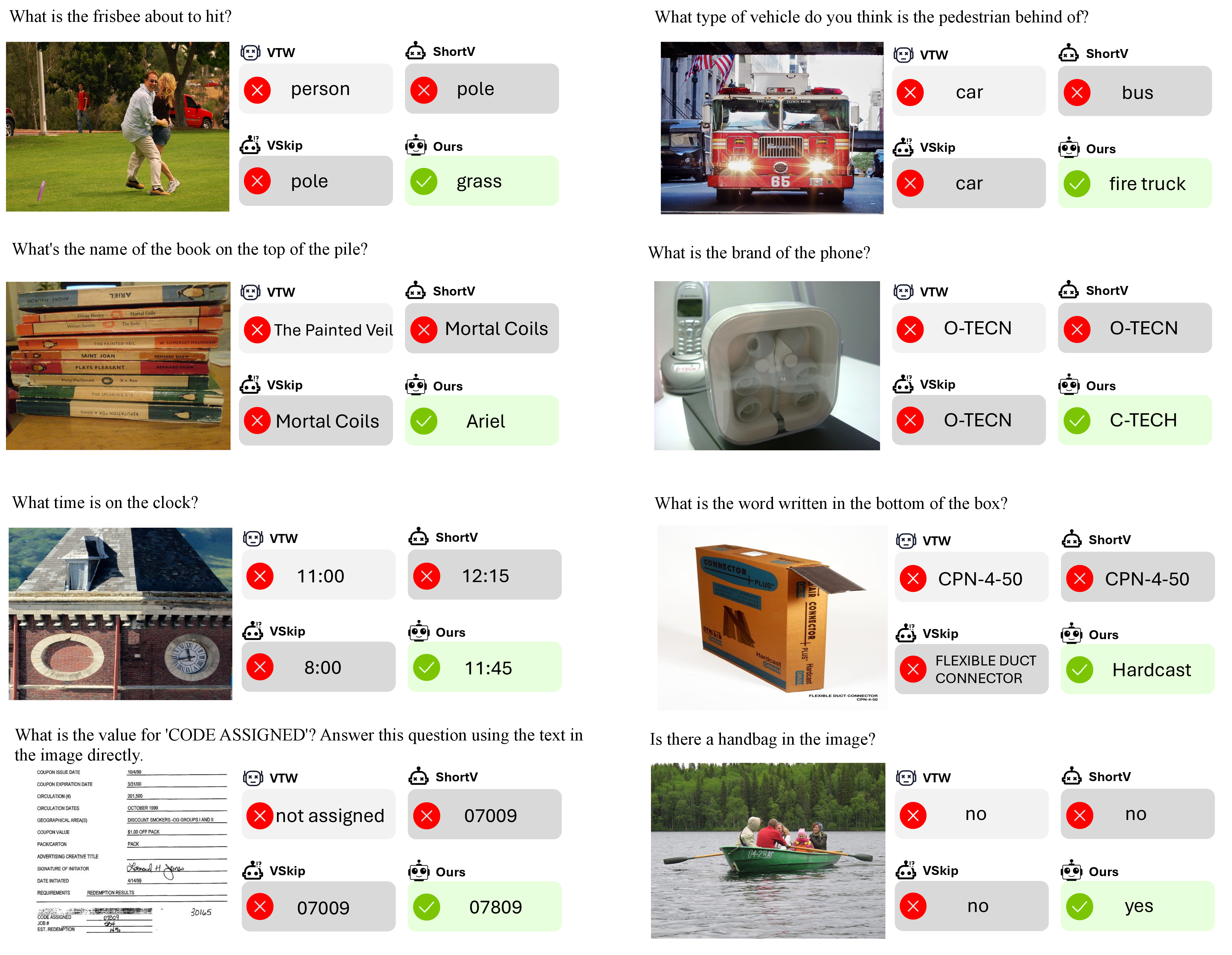
Figure 5 visualizes model responses under operator-aware visual-token skipping. Our method still produces accurate answers on both reasoning and recognition examples, suggesting that it preserves the operators responsible for key layer-wise visual reasoning functions and largely maintains the model’s answer quality.
4.4 Effect of Operator-Skipping Budget↩︎
We study how the operator-skipping budget affects performance across the three evaluated MLLMs. As shown in Table 3, moderate budgets simplify redundant visual computation through Attention-only, FFN-only, or Freeze-update while preserving most benchmark scores, whereas overly aggressive budgets eventually degrade performance on fine-grained or text-rich tasks. This consistent trend across LLaVA-1.5-7B, Qwen2.5-VL-7B, and Qwen3-VL-8B suggests that operator-level redundancy is broadly present, but the best budget remains model-dependent and should be treated as an efficiency–performance knob.
4.5 Ablation Study↩︎
To isolate the contribution of operator-aware policy assignment, we conduct a fixed-budget ablation on Qwen3-VL-8B with budget \(B=28\). All variants simplify the same number of layers, but use different operator actions, Attn-Skip always skips visual attention, FFN-Skip always skips visual FFN, and Frozen skips both operators. As shown in Table 5, fixed rules are not uniformly reliable, while our layer-wise risk-based assignment better balances efficiency and accuracy by matching the skipped operator to each layer’s dominant visual operator.
| Method | GQA | POPE | MME | OCRB | VizWiz |
|---|---|---|---|---|---|
| Vanilla | 61.6 | 89.1 | 2390 | 82.8 | 69.4 |
| Attn-Skip | 53.6 | 78.6 | 1506 | 11.2 | 58.8 |
| FFN-Skip | 59.6 | 89.3 | 2118 | 61.7 | 66.2 |
| Frozen | 26.8 | 57.1 | 975 | 20.0 | 52.3 |
| Ours | 60.0 | 89.2 | 2159 | 76.4 | 69.1 |
4.6 Combination with Token Pruning↩︎
Finally, we study whether operator-aware skipping is complementary to token pruning. Token pruning reduces the visual sequence length, while our method removes redundant operator computation on the remaining tokens, so the two strategies target different sources of redundancy. As shown in Table 6, applying our method on top of VisionZip [11] or V2Drop [26] further reduces computation while preserving answer quality better than more aggressive pruning. This suggests that, especially in the low-token regime, retaining more visual evidence and skipping redundant operators is preferable to further shortening the visual sequence.
| Method (Token Ret.) | TFLOPs | GQA | TextVQA | MME | MMB | POPE |
|---|---|---|---|---|---|---|
| VisionZip (\(10\%\)) | 1.67 | 49.8 | 61.0 | 1717.1 | 69.0 | 79.5 |
| VisionZip (\(3\%\)) | ||||||
| VisionZip + Ours (\(10\%\)) | ||||||
| V2Drop (\(10\%\)) | 2.59 | 54.7 | 60.4 | 2012.6 | 77.7 | 86.5 |
| V2Drop (\(2\%\)) | ||||||
| V2Drop + Ours (\(10\%\)) |
4.7 Qualitative Comparison↩︎
Figure 5 shows that operator-aware visual-token skipping preserves accurate responses on examples requiring visual reasoning and object recognition. These qualitative results suggest that our policy maintains answer capability while removing redundant visual computation.
5 Conclusion↩︎
We demonstrated that visual redundancy in MLLMs is answer-observable and operator-dependent, with late visual-token updates often contributing little to answers. Our operator-aware skipping preserves all visual tokens while bypassing redundant attention, FFN, or both, reducing visual computation across multiple backbones with little performance loss, without irreversible evidence loss from pruning.
6 Related Work↩︎
6.0.0.1 Layer-wise visual-computation skipping.
As high-resolution inputs, image tiling, and dense visual encoders increase the length of visual prefixes, the LLM prefill stage has become a major bottleneck for MLLM inference [7], [12]–[14]. One line of work reduces this cost by modifying how visual tokens are processed across Transformer layers. VTW withdraws visual tokens from later layers to avoid repeatedly propagating visual states through the full LLM backbone [13], while ShortV freezes visual-token states in layers identified as visually ineffective [12]. V-Skip studies block-wise attention skipping and shows that visual attention computation can be redundant in selected layers [14]. Related structural acceleration methods also exploit layer-wise or block-wise redundancy to reduce visual computation without directly deleting all visual inputs [7], [14]. Together, these studies show that visual computation can be redundant in a depth-dependent manner, but they differ in the granularity at which redundancy is modeled. VTW and ShortV primarily act on full visual-token states, whereas V-Skip focuses on attention computation. Our work is complementary, instead of treating a layer or a single operator family as the default unit of analysis, we compare the answer-observable risks of visual-row attention and visual-row FFN within each layer. This operator-level view allows the policy to preserve the operator that remains useful at a given depth while skipping the redundant one, or to freeze the visual update when both operators are answer-silent.
6.0.0.2 Visual-token pruning and compression.
Another major direction accelerates MLLM inference by reducing the number of visual tokens. Early and recent methods prune, merge, or select visual tokens according to attention scores, token similarity, spatial redundancy, diversity, or output sensitivity [7], [9]–[11], [26]–[29]. These approaches directly shorten the visual sequence and can reduce both attention and FFN costs in subsequent layers. However, token reduction is inherently destructive, once visual tokens are removed, merged, or prematurely withdrawn, the corresponding spatial evidence cannot be recovered by later textual reasoning. This limitation is especially pronounced in fine-grained recognition tasks, including OCR-centric VQA, chart or diagram understanding, small-object reasoning, and visually grounded question answering, where the decisive evidence may occupy only a small image region or become relevant only after interacting with the question. Recent studies further show that aggressive token pruning can damage spatial integrity, shift relevant visual information during decoding, and even underperform random selection in certain settings [8], [30]–[32]. In contrast, our method preserves the full visual-token sequence throughout inference and reduces computation at the operator level. This avoids irreversible loss of fine-grained visual evidence while still removing answer-silent visual updates, matching the motivation in the introduction: efficient MLLM inference should preserve visual information and reduce only computation that is not observable from the answer side.
7 Implementation Environment↩︎
All experiments were conducted on an internal GPU cluster equipped with NVIDIA A800-SXM4 GPUs. Each compute node contains two Intel(R) Xeon(R) Platinum 8358 CPUs at 2.60GHz, providing 128 logical CPU cores in total, approximately 1 TiB of system memory, and 8 NVIDIA A800-SXM4 GPUs with 80GB VRAM each. The NVIDIA driver version is 535.161.08. The system CUDA toolkit is CUDA 12.2, while the PyTorch binaries used in our conda environments are built with CUDA 12.1.
| Model family | Python | PyTorch | Torchvision | Transformers | Accelerate | lmms-eval |
|---|---|---|---|---|---|---|
| Qwen2-VL | 3.12.12 | 2.4.1 | 0.19.1 | 4.51.3 | 1.13.0 | 0.6.1 |
| Qwen3-VL | 3.12.12 | 2.4.1 | 0.19.1 | 5.5.4 | 1.13.0 | 0.6.1 |
| LLaVA-1.5 | 3.12.9 | 2.4.1 | 0.19.1 | 4.37.2 | 0.21.0 | 0.6.1 |
| LLaVA-NeXT | 3.10.20 | 2.1.2+cu121 | 0.16.2+cu121 | 4.40.0.dev0 | 0.29.3 | 0.6.1 |
We use the official lmms-eval framework for all reported multimodal benchmark results and follow its default evaluation protocols. Since different model families rely on different dependency constraints, we maintain separate conda
environments for Qwen2-VL, Qwen3-VL, LLaVA-1.5, and LLaVA-NeXT. Model checkpoints are loaded from local copies of the corresponding public Hugging Face repositories. The evaluated benchmark suite includes MME, MMBench, OCRBench, POPE, GQA, TextVQA,
ScienceQA, MMMU, AI2D, and VizWiz when applicable.
| Model family | Qwen2.5VL | Qwen3VL | Llava1.5 | Llava-Next |
|---|---|---|---|---|
| datasets | 2.16.1 | 2.16.1 | 2.16.1 | 5.0.0 |
| tokenizers | 0.21.4 | 0.22.2 | 0.15.1 | 0.15.2 |
| sentencepiece | 0.2.1 | 0.2.1 | 0.2.1 | 0.2.1 |
| qwen-vl-utils | 0.0.14 | 0.0.14 | – | – |
| llava | – | – | 1.2.2.post1 | 1.7.0.dev0 |
8 Computation of Answer-Observable Metrics↩︎
In Section 2, we define answer-observable influence (AOI) using the exact Jacobian from visual-token states to the final prompt-token hidden state. This definition is mathematically direct, but computing the full Jacobian is prohibitively expensive for modern MLLMs. We therefore estimate AOI with randomized probes. This section derives the estimator used in our implementation.
Let \(H_v^{l+1} \in \mathbf{R}^{N_v \times d}\) denote the visual-token hidden states after layer \(l\), and let \[\Delta V_l = H_v^{l+1} - H_v^l\] be the visual-token update. We write \(v_l=\mathrm{vec}(\Delta V_l)\) for its flattened representation. Let \(h_{\mathrm{last}}\in\mathbf{R}^{d}\) be the final prompt-token hidden state after prefill, and let \[J_l = \frac{\partial h_{\mathrm{last}}}{\partial \mathrm{vec}(H_v^{l+1})} \in \mathbf{R}^{d \times N_vd}\] be the Jacobian mapping perturbations of visual-token states at layer \(l+1\) to perturbations of the final prompt-token hidden state. The exact first-order change induced by the visual update is \[\delta h_l = J_l v_l,\] and the exact answer-observable influence is \[\mathrm{AOI}_l = \|\delta h_l\|_2 = \|J_l v_l\|_2 .\] Directly forming \(J_l\) is infeasible because it has size \(d \times N_vd\). Instead, we estimate the norm of \(J_l v_l\) through random projections.
Let \(r_k \in \mathbf{R}^{d}\) be an independent random probe satisfying \[\mathbf{E}[r_k r_k^\top] = I_d .\] In practice, \(r_k\) can be sampled from a standard Gaussian distribution or a Rademacher distribution. For each probe, we define \[g_{l,k} = \left\langle \frac{\partial (r_k^\top h_{\mathrm{last}})}{\partial H_v^{l+1}}, \Delta V_l \right\rangle_F .\] This quantity can be computed with a single reverse-mode gradient call, without explicitly constructing the full Jacobian. By the chain rule, \[\frac{\partial (r_k^\top h_{\mathrm{last}})}{\partial \mathrm{vec}(H_v^{l+1})} = J_l^\top r_k .\] Therefore, \[g_{l,k} = \langle J_l^\top r_k, v_l\rangle = r_k^\top J_l v_l = r_k^\top \delta h_l .\] Thus, \(g_{l,k}\) is a random projection of the exact answer-side perturbation \(\delta h_l\).
The squared projection gives an unbiased estimator of the squared AOI: \[\begin{align} \mathbf{E}_{r_k}[g_{l,k}^2] &= \mathbf{E}_{r_k} \left[(r_k^\top \delta h_l)^2\right] \\ &= \delta h_l^\top \mathbf{E}[r_k r_k^\top] \delta h_l \\ &= \|\delta h_l\|_2^2 \\ &= \mathrm{AOI}_l^2 . \end{align}\] With \(K\) independent probes, we estimate AOI as \[\widehat{\mathrm{AOI}}_l = \left( \frac{1}{K} \sum_{k=1}^{K} g_{l,k}^2 \right)^{1/2}.\] This estimator is consistent for \(\mathrm{AOI}_l\) as \(K\) increases, while requiring only vector-Jacobian products rather than the full Jacobian. In our diagnostic figures, the plotted AOI is computed using this randomized estimator.
After estimating AOI, we compute answer-observable efficiency (AOE) by normalizing the estimated answer-observable influence by the visual update magnitude: \[\widehat{\mathrm{AOE}}_l = \frac{ \widehat{\mathrm{AOI}}_l }{ \|\Delta V_l\|_F + \epsilon } .\] For visualization across layers, we further normalize AOE within each model and dataset: \[\widetilde{\mathrm{AOE}}_l = \frac{ \widehat{\mathrm{AOE}}_l }{ \max_j \widehat{\mathrm{AOE}}_j + \epsilon } .\]
| Model | Method | TFLOPs | GQA | TextVQA | MME | MMB | MMMU | POPE | SQA | AI2D | OCRB | VizWiz | Avg. Ret. |
|---|---|---|---|---|---|---|---|---|---|---|---|---|---|
| LLaVA-NeXT | Vanilla | 100% | 64.30 | 61.36 | 1851.44 | 67.10 | 36.00 | 87.61 | 70.15 | 65.35 | 52.20 | 60.75 | 100.0 |
| VTW (K=16) | 51% | 55.41 | 47.71 | 1852.56 | 66.75 | 35.56 | 87.41 | 70.00 | 65.38 | 6.90 | 54.86 | 86.5 | |
| ShortV (N=20) | 51% | 62.83 | 56.50 | 1854.51 | 66.92 | 35.89 | 87.38 | 69.26 | 64.48 | 41.40 | 57.09 | 96.0 | |
| VSkip+ (N=20) | 74% | 63.31 | 59.74 | 1759.67 | 67.01 | 36.22 | 87.35 | 69.83 | 65.25 | 48.80 | 59.35 | 98.2 | |
| V2Drop | 70% | 62.58 | 59.83 | 1853.23 | 67.25 | 36.00 | 87.98 | 69.92 | 64.75 | 50.30 | 56.83 | 98.4 | |
| APET | 70% | 62.97 | 59.98 | 1840.33 | 67.18 | 37.11 | 87.79 | 69.71 | 65.01 | 50.60 | 60.72 | 99.4 | |
| Ours (N=20) | 67% | 63.01 | 60.65 | 1797.57 | 66.75 | 36.78 | 88.31 | 69.96 | 65.03 | 50.60 | 57.99 | 98.8 |
Therefore, VUM measures how much visual-token states move, AOI estimates how much this movement reaches the final prompt-token hidden state, and AOE measures the answer-observable influence induced per unit visual update.
In implementation, we first run the original model forward pass and cache \(H_v^l\), \(H_v^{l+1}\), and \(h_{\mathrm{last}}\) for each layer. For each layer \(l\), we sample \(K\) random probes \(\{r_k\}_{k=1}^K\), compute the scalar \(r_k^\top h_{\mathrm{last}}\), backpropagate it to obtain the gradient with respect to \(H_v^{l+1}\), and take its Frobenius inner product with \(\Delta V_l\). Model parameters are kept frozen, and no ground-truth answer labels are used. This makes the diagnostic label-free and applicable to arbitrary multimodal prompts.
9 Experiments on LLaVA-NeXT↩︎
To further test architectural generality, we additionally evaluate on LLaVA-NeXT. Compared with LLaVA-1.5, LLaVA-NeXT uses stronger visual processing and is commonly evaluated under higher-resolution or multi-image settings, making visual-token computation more expensive. This provides a useful stress test for operator-aware skipping because high-resolution visual inputs amplify the cost of repeatedly updating visual-token representations inside the LLM backbone.
Table 9 shows that our method remains effective in this higher-resolution setting. With \(67\%\) TFLOPs, our method preserves \(98.8\%\) average performance and achieves the best results among non-vanilla methods on TextVQA and POPE, while also ranking second on GQA, MMMU, and SQA. It also matches the best OCRBench score. These results indicate that the operator-level redundancy identified in the main experiments is not limited to the three primary backbones, but also appears in LLaVA-NeXT. Even when the visual input is more expensive to process, selectively skipping redundant visual operators can reduce computation while maintaining strong benchmark performance.
10 Calibration Sample Size Study↩︎
We study how the number of calibration samples from each benchmark affects the analysis decisions made by our method. For each of the seven calibration benchmarks used in the main experiments, we randomly sample \(8\), \(16\), or \(20\) examples and estimate the layer-wise operator risks for LLaVA-1.5-7B, Qwen2.5-VL-7B, and Qwen3-VL-8B. The resulting risk profile determines the selected layers and their operator-skipping policies, and the same policy is then evaluated on the full benchmark suite.
Table 6 reports the average retention under different layer budgets. The goal is to test whether using more calibration samples leads to a substantially more reliable policy. Since calibration is used only for risk estimation and does not require labels or model training, a small sample size is desirable if it already supports stable policy selection.
Figure 6: 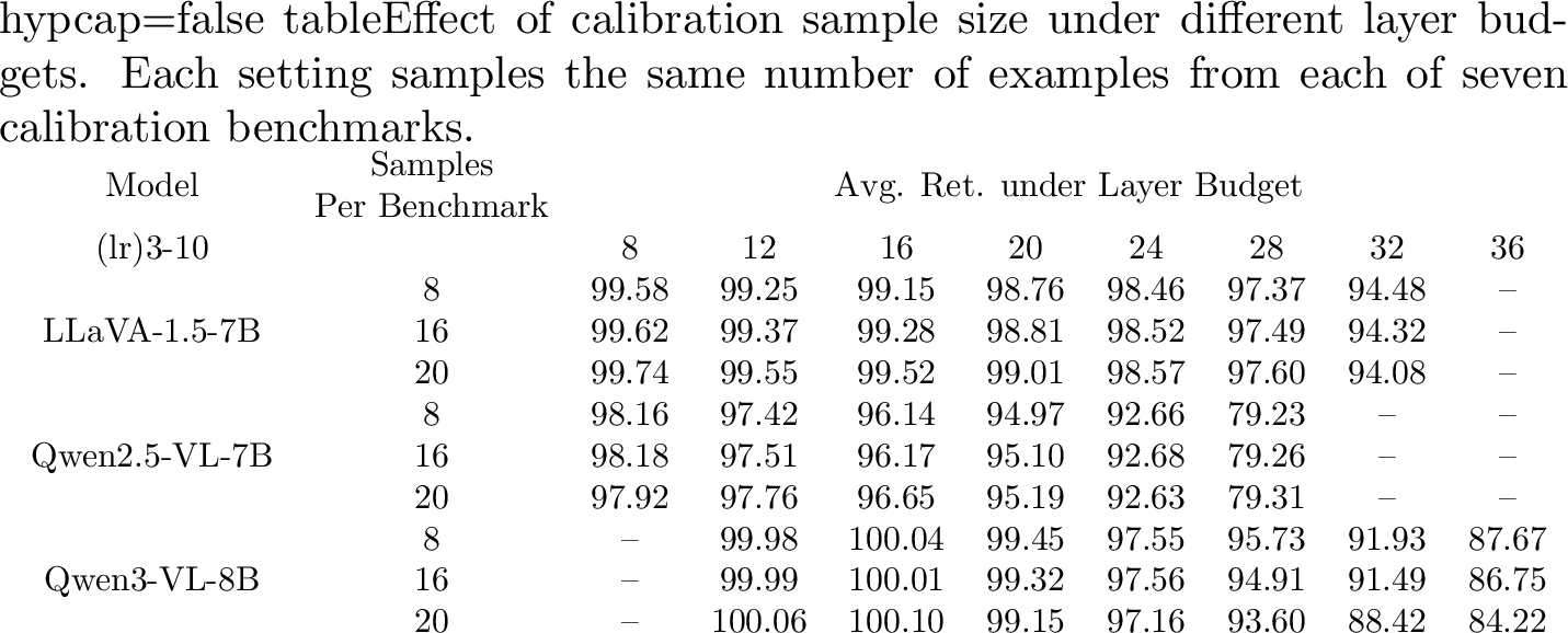 .
.
The results show that increasing the number of calibration samples can bring improvements at some layer budgets, but the gains are not consistently large or monotonic. For example, more samples slightly improve several LLaVA-1.5-7B settings, while the trends for Qwen2.5-VL-7B and Qwen3-VL-8B vary across budgets. This suggests that \(8\) samples per benchmark are already sufficient to support the risk analysis used by our method. Adding more samples can provide stronger evidence in some cases, but it is not always necessary for obtaining stable operator-skipping decisions.
11 Ablation on Risk-Based Layer Allocation↩︎
We compare our budgeted layer allocation with a simple last-layer heuristic. As described in Section 3.2, our policy first ranks layers by the summed single-operator risk \(\mathcal{R}_{\mathcal{A}}(l)+\mathcal{R}_{\mathcal{F}}(l)\) and allocates the skipping budget to the lowest-risk layers. This design assumes that layers with smaller summed risk can safely discard their non-dominant visual operator earlier, whereas layers with larger summed risk should be postponed because even their non-dominant operator may still affect the output.
Figure 8:  .
.
This ablation isolates the effect of this layer-allocation rule. For both methods, we keep the per-layer operation type fixed; each selected layer uses the same skip-operator decision or the same frozen update determined by the operator-risk profile. The only difference is which layers are selected. Our method selects the 20 layers with the smallest \(\mathcal{R}_{\mathcal{A}}(l)+\mathcal{R}_{\mathcal{F}}(l)\), while the Last-20 heuristic directly selects the final 20 Transformer layers regardless of their risk scores. Table 8 reports the Qwen3-VL-8B comparison, testing whether risk-based allocation is preferable to choosing late layers purely by position.
The results support our hypothesis. With the same number of selected layers and the same per-layer operator actions, risk-based allocation consistently outperforms the Last-20 heuristic across all reported benchmarks. This indicates that small-\(\mathcal{R}_{\mathcal{A}}+\mathcal{R}_{\mathcal{F}}\) layers are indeed safer places to discard non-dominant visual operators, while simply choosing the final layers may remove useful visual computation whose operator risk remains high.
12 Different Budget of Our Method↩︎
Table [tbl:tab:app95budget] studies how the operator-skipping budget affects performance across four MLLM backbones. Overall, the results show that our operator-aware policy is not tied to a particular architecture, LLaVA-1.5, LLaVA-NeXT, Qwen2.5-VL, and Qwen3-VL all maintain high average retention under moderate budgets, despite their different visual encoders, language backbones, and dependency stacks. In particular, small and medium budgets usually preserve nearly all vanilla performance, and several individual benchmarks even improve over the budget-0 setting. This suggests that the skipped operators are often answer-silent rather than uniformly useful, supporting the reliability of the proposed answer-observable selection criterion.
The budget trend also reveals a consistent efficiency–accuracy pattern. As the budget increases, average retention decreases smoothly rather than collapsing abruptly, indicating that the policy removes redundant visual computation in a controlled manner. This behavior is especially important for practical deployment, users can choose conservative budgets when accuracy is the priority, or larger budgets when higher efficiency is needed. Across all models, moderate budgets retain strong performance, while aggressive settings expose the trade-off when too much visual computation is skipped. These results show that operator-level visual skipping is broadly applicable and robust under different layer-level budgets.
References↩︎
The source code is available at: https://github.com/zayan-l/Op-Skip.↩︎