Relational and Sequential Conformal Inference for Energy Time Series over Graphs via Foundation Models
June 30, 2026
Abstract
Accurate energy demand forecasting is essential for the reliable operation and planning of modern sustainable energy systems. Spatial-temporal graph neural networks (STGNNs) have recently achieved strong performance in point forecasting by jointly modeling temporal dynamics and relational dependencies across interconnected energy nodes. However, in real-world energy systems, accurate point forecasts alone are insufficient, as operators also require reliable uncertainty estimates to support risk-aware decision-making, grid stability, and operational planning under uncertainty. Conformal prediction provides a principled and model-agnostic framework for uncertainty quantification with statistical coverage guarantees, making it particularly attractive for safety-critical energy applications. However, existing conformal prediction approaches often fail to fully capture the complex spatial-temporal structure of energy systems. To address these limitations, we propose STOIC (Spatial-Temporal Graph Conformal Prediction with In-Context Learning), a novel framework that integrates graph-based forecasting with the zero-shot calibration capabilities of tabular foundation models. STOIC first generates point forecasts using an STGNN and subsequently reformulates spatial-temporal residuals into a tabular representation suitable for in-context learning. Leveraging a tabular foundation model, STOIC calibrates prediction intervals without task-specific retraining, effectively capturing both sequential and relational dependencies. We evaluate STOIC on five diverse benchmarks, including synthetic simulations as well as real-world electricity and district heating networks. Across all datasets, STOIC consistently outperforms existing conformal prediction baselines, delivering more reliable and robust uncertainty estimates for complex graph-structured energy time series.
1 Introduction↩︎
Accurate energy demand forecasting is becoming increasingly critical with the rapid integration of renewable energy sources, the electrification of heating, and the growing complexity of smart energy systems [1], [2]. Reliable forecasts of electricity and heating demand are essential for a wide range of operational and planning tasks, including generation scheduling, storage management, district heating operation, demand response, and long-term infrastructure planning [3], [4]. As modern energy systems become more decentralized and weather-dependent, forecasting errors can propagate through interconnected infrastructures and directly affect system stability, operational efficiency, and economic cost. Over the past decade, deep learning approaches have significantly advanced forecasting performance by learning complex nonlinear temporal patterns from large historical datasets [5]–[7]. Architectures based on recurrent neural networks [8], temporal convolutions [9], and transformer models [10], [11] have demonstrated strong predictive capabilities across a variety of electricity and heating applications, establishing deep learning as a dominant paradigm for energy forecasting.
Despite these advances, most existing forecasting models focus primarily on temporal dynamics and often treat each location or asset independently. In real-world energy systems, however, demand patterns are inherently interconnected [12]. Electricity consumption and heating load are influenced by spatial proximity, shared weather conditions, socio-economic factors, and correlated human activity [13]. As a result, models that ignore spatial dependencies may fail to capture important relational information and overlook how demand at one node influences neighboring regions [14]. This issue is especially pronounced in district heating networks and geographically distributed electricity systems, where demand dynamics exhibit strong spatial coupling [15]. Consequently, even highly accurate temporal models may miss a critical source of predictive information.
Graph neural networks (GNNs) provide a natural framework for modeling these dependencies [16]. By representing energy systems as graphs, GNNs explicitly encode relationships between interconnected nodes and learn how information propagates across the network [17], [18]. Combined with temporal modeling components, spatial-temporal graph neural networks (STGNNs) have achieved promising results in forecasting tasks where both local temporal dynamics and network interactions are important [19]. Such models are particularly well suited to energy applications [20], [21], as they can jointly exploit topological structure, neighborhood influence, and system-wide interactions within a unified architecture [22], [23]. However, accurate point forecasts alone are insufficient for real-world energy system operation. While STGNNs substantially improve predictive accuracy, they remain fundamentally deterministic models that provide only single-valued forecasts without quantifying the uncertainty associated with future demand. In operational settings, forecasting uncertainty is often as important as forecasting accuracy itself. Energy operators must continuously make high-stakes decisions under incomplete and evolving information, where inaccurate confidence estimates can directly affect reserve allocation, storage scheduling, market participation, and overall system reliability.
Accurate uncertainty quantification is therefore essential for risk-aware energy management [24]. Underestimating uncertainty can lead to inadequate reserve allocation, inefficient storage utilization, unstable scheduling decisions, and reduced system reliability. Conversely, overly conservative estimates may result in unnecessary operational costs and inefficient resource usage. Recent works discuss uncertainty classification from both system and modeling perspectives [25]–[27], distinguishing between aleatoric uncertainty (irreducible data variability) and epistemic uncertainty (reducible lack of knowledge); when the model is misspecified, aleatoric uncertainty cannot be properly quantified, resulting in strongly coupled parameter uncertainties and model discrepancies. To handle these coupled uncertainties, classical Bayesian inference frameworks [28], [29], which are implemented via sampling [30] or variational approaches [25], [31], are utilized alongside Gaussian processes [32]–[35] and Bayesian neural networks [36]–[39] to provide principled probabilistic interpretations and posterior distributions over predictions. While these models are highly attractive when epistemic uncertainty is important [40], enabling operators to assess forecast confidence and make robust decisions in weather-dependent sustainable energy systems [41], they are often hindered by restrictive distributional assumptions that fail under regime-shifting energy demand data. Furthermore, because these probabilistic methods can be computationally demanding for large-scale spatial-temporal datasets [42], [43], there is a growing motivation to develop distribution-free uncertainty quantification methods that remain reliable under complex spatial-temporal dependencies.
Conformal Prediction (CP) is a well-established distribution-free alternative for uncertainty quantification [44]. Rather than identifying or specifying the source of uncertainty, it yields prediction intervals with coverage guarantees on a certain quantity of interest based on observed data on the same quantity. Unlike Bayesian approaches, CP does not require strong assumptions about the underlying data-generating process [45]. Instead, it constructs prediction intervals with finite-sample coverage guarantees under minimal assumptions, making it particularly appealing for real-world energy applications where distributional assumptions are often difficult to verify. CP also acts as a flexible wrapper that can be combined with arbitrary forecasting models to produce calibrated uncertainty estimates. However, standard conformal methods typically assume exchangeability [46], an assumption that is often violated in energy systems due to temporal dependencies and spatial correlations across interconnected nodes. As a consequence, naive conformal approaches may produce intervals that are either miscalibrated or overly conservative.
Several recent methods attempt to address these limitations. Adaptive Conformal Inference (ACI) [47] and Sequential Predictive Conformal Inference (SPCI) [48] improve calibration under temporal non‑stationarity but still treat each time series independently, ignoring relational interactions between nodes. Spatial approaches such as Localized Spatial Conformal Prediction (LSCP) [49] incorporate spatial structure, yet are designed for static spatial settings and do not explicitly model temporal dependencies. More recent graph-based approaches estimate uncertainty through relational modeling using quantile random forests with the residual history of neighboring nodes as input features [50], quantile GNNs [51], or ellipsoidal sets prediction sets that capture pairwise node dependencies [52]. Nevertheless, these approaches generally require retraining or calibration procedures whenever the deployment setting changes. This dependency limits scalability and reduces adaptability across heterogeneous energy systems, where new networks, operating regimes, or calibration windows may frequently arise.
Tabular Foundation Models (FMs) have recently demonstrated strong in-context learning capabilities, enabling them to generalize to new structured tasks with minimal additional data [53]–[55]. We leverage this capability for scalable uncertainty calibration: rather than designing specialized calibration procedures for each forecasting task, these pretrained models can perform task-specific inference without explicit retraining [56], [57], making them especially desirable for reducing calibration overhead in dynamic forecasting environments. While dedicated FM for spatial-temporal graph forecasting remains limited, recent successes in tabular learning with models such as TabPFN [58], [59] demonstrate strong in-context learning capabilities on structured data. This creates an opportunity to reformulate the calibration stage, rather than the full forecasting problem, into a structured tabular representation. Motivated by this perspective, spatial-temporal residuals can be organized in tabular form and calibrated using pretrained tabular foundation models, enabling efficient conformal calibration without modifying the underlying forecasting architecture.
Building on this idea, we propose Spatial-Temporal Graph Conformal Prediction with In-Context Learning (STOIC), a novel framework for uncertainty quantification in graph-based energy forecasting. STOIC first trains an STGNN to generate point forecasts over spatial-temporal energy networks. The residuals produced by the pretrained forecasting model are then transformed into a structured tabular representation that captures temporal dependencies through local residual history and rolling statistics, and relational dependencies through permutation-invariant aggregators (e.g., mean, median, min, max) over neighbors’ residuals, which is directly inspired by the message-passing framework. A pretrained tabular FM is subsequently employed to calibrate these residuals and construct prediction intervals without task-specific retraining. In this way, STOIC combines the representational power of spatial-temporal graph modeling with the data efficiency of in-context learning to produce reliable and transferable uncertainty estimates.
To evaluate the proposed framework, we conduct experiments on five datasets spanning both synthetic and real-world settings. These benchmarks include controlled simulations, synthetic district heating networks, real-world district heating systems, and real-world electricity demand datasets. Across these diverse scenarios, STOIC consistently produces calibrated and efficient prediction intervals while remaining robust to complex spatial-temporal dependencies and non-stationary dynamics.
The main contributions of this paper are summarized as follows:
We propose STOIC, a novel CP framework that combines spatial-temporal graph forecasting with the zero-shot calibration capabilities of tabular FMs.
We develop a methodology for transforming spatial-temporal forecasting residuals into structured tabular representation, enabling in-context learning for conditional quantile estimation.
We demonstrate that pretrained tabular FMs such as TabPFN can be leveraged to construct robust and calibrated prediction intervals that capture complex spatial-temporal dependencies without task-specific retraining.
We perform extensive experiments across five synthetic and real-world energy datasets, demonstrating that STOIC consistently achieves more reliable and efficient uncertainty estimates than existing conformal prediction baselines.
The remainder of this paper is organized as follows. Section 2 introduces the necessary preliminaries and background concepts. Section 3 presents the proposed STOIC framework. Sections 4 and 5 report the experimental setup and results, respectively. Finally, Section 6 concludes the paper and discusses future research directions.
2 Preliminaries↩︎
This section introduces the foundational concepts required to understand the STOIC framework. We first establish the mathematical notation for spatial-temporal energy demand forecasting and define the objectives for both point forecasting and uncertainty quantification. We then provide an overview of CP, a distribution-free framework that serves as the theoretical foundation of the proposed calibration approach. Finally, we discuss the key challenges associated with applying uncertainty quantification methods to spatial-temporal graph-structured energy demand data.
2.1 Problem Formulation and Uncertainty Quantification↩︎
We consider a spatial-temporal energy demand forecasting problem over a network of \(N\) interconnected nodes. Let \(x_{i,t}\) denote the scalar observation at node \(i\) and time \(t\). In real-world settings, these observations are subject to measurement noise and other sources of stochasticity, which introduce additional uncertainty into the forecasting task. The observations across all nodes at time \(t\) are represented by the vector \(\mathbf{x}_t = [x_{1,t}, x_{2,t}, \dots, x_{N,t}]^\top.\) Given a historical observation window of length \(W\), the forecasting model receives as input the sequence \(\mathbf{X}_{t-W:t-1} = [\mathbf{x}_{t-W}, \dots, \mathbf{x}_{t-1}] \in \mathbb{R}^{N \times W},\) which captures both the temporal evolution of each node and the interactions across the network over the past \(W\) time steps. The objective is to predict the future demand vector at time \(t\): \[\hat{\mathbf{x}}_{t} = f_\theta(\mathbf{X}_{t-W:t-1}),\] where \(f_\theta\) denotes a forecasting model parameterized by \(\theta\). The prediction corresponding to node \(i\) is given by the \(i\)-th component of the forecast vector: \[\hat{x}_{i,t} = [\hat{\mathbf{x}}_{t}]_i.\]
While accurate point forecasting is important, operational decision-making in energy systems also requires reliable estimates of predictive uncertainty. To this end, the goal is to construct prediction intervals (PIs) of the form: \[C_{i,t}^\alpha = [\ell_{i,t}^\alpha, u_{i,t}^\alpha],\] where \(\ell_{i,t}^{\alpha}\) and \(u_{i,t}^{\alpha}\) denote the lower and upper bounds of the interval for node \(i\) at time \(t\), respectively, and \(\alpha \in (0,1)\) is a user-specified target miscoverage level; a smaller \(\alpha\) enforces higher confidence but typically results in wider prediction intervals. Ideally, the prediction intervals should satisfy the coverage property \[\mathbb{P}(x_{i,t} \in C_{i,t}^\alpha) \ge 1 - \alpha,\] commonly referred to as marginal coverage [60]. A stronger requirement is conditional coverage [60], which conditions on the observed historical context: \[\mathbb{P}(x_{i,t} \in C_{i,t}^\alpha \mid \mathbf{X}_{t-W:t-1}) \ge 1 - \alpha.\]
Achieving conditional coverage is substantially more challenging in spatial-temporal forecasting settings due to temporal dependencies, spatial correlations, and distributional shifts across nodes and time horizons.
In this work, we focus on post-hoc uncertainty quantification, where calibrated prediction intervals are constructed on top of an already trained forecasting model. This setting is especially attractive in practice because it avoids modifying or retraining the underlying forecasting architecture, thereby preserving the predictive capabilities of the pretrained forecaster while augmenting it with reliable uncertainty estimates.
2.2 Conformal Prediction↩︎
Conformal prediction (CP) is a distribution-free framework for uncertainty quantification that constructs calibrated PIs using empirical quantiles of conformity scores. A key advantage of CP is that it can be applied as a post-hoc wrapper around arbitrary forecasting models while providing finite-sample coverage guarantees under relatively mild assumptions [44]. In this work, we adopt the split conformal prediction (SCP) setting [61], where the available data is partitioned into disjoint training and calibration sets. The forecasting model is first trained on the training set, while the calibration set is subsequently used to estimate the distribution of prediction errors and construct calibrated uncertainty intervals.
Let \(\mathcal{T}_{\mathrm{cal}}\) denote a set of \(n\) calibration time indices, disjoint from the training set. For each calibration time step \(t \in \mathcal{T}_{\mathrm{cal}}\), the forecasting model produces the prediction: \[\hat{\mathbf{x}}_{t} = f_\theta(\mathbf{X}_{t-W:t-1}),\] where \(f_\theta\) denotes the pretrained forecasting model. The corresponding residual vector is defined as: \[\mathbf{r}_{t} = \mathbf{x}_{t} - \hat{\mathbf{x}}_{t}.\] The residual associated with node \(i\) is therefore given by: \[r_{i,t} = [\mathbf{r}_{t}]_i.\] Following standard SCP, the conformity score is defined as the absolute prediction residual: \[s_{i,t} = \left|r_{i,t}\right|.\]
Given a target miscoverage level \(\alpha \in (0,1)\), the conformal quantile for node \(i\) is estimated from the calibration conformity scores: \[\hat{q}_{i}^{1-\alpha} = \mathrm{Quantile}_{\lceil (n+1)(1-\alpha) \rceil}(\{s_{i,t} \}_{t \in \mathcal{T}_{\mathrm{cal}}}).\] The resulting PI for a new test sample at time \(t^\prime\) is then constructed as: \[C_{i,t^\prime}^\alpha = \left[\hat{x}_{i,t^\prime} - \hat{q}_{i}^{1-\alpha}, \; \hat{x}_{i,t^\prime} + \hat{q}_{i}^{1-\alpha}\right].\]
Under the assumption that the calibration and test residuals are exchangeable [46], SCP guarantees the marginal coverage property introduced previously. However, this assumption is often violated in spatial-temporal forecasting problems due to temporal dependencies, distributional shifts, and correlations across interconnected nodes. Consequently, standard conformal approaches produce intervals that are either miscalibrated or overly conservative. The central objective of this work is therefore to move beyond independent residual calibration and exploit the structured dependencies present in spatial-temporal energy demand data. Rather than treating calibration residuals as isolated samples, the proposed framework leverages temporal and relational information to construct more informative and adaptive prediction intervals.
2.3 Graph Deep Learning for Point Forecasting↩︎
STGNNs provide a natural framework for forecasting energy demand over interconnected systems. Their fundamental principle is to jointly model temporal dynamics at individual nodes and relational dependencies across the underlying network. By combining temporal representation learning with graph-based message passing, STGNNs can capture both local consumption dynamics and cross-node interactions within a unified architecture. In STOIC, the STGNN serves as the point forecasting backbone prior to uncertainty quantification.
We adopt a time-then-space architecture [51], [62], in which temporal dependencies are first encoded independently by a sequence encoder at each node before spatial interactions are incorporated through graph propagation layers. For each node \(i\), the temporal encoder processes this historical sequence \(\mathbf{x}_{i,t-W:t-1} \in \mathbb{R}^{W},\) and maps it to a latent representation: \[\mathbf{h}^{(0)}_{i,t} = \mathrm{TemporalEncoder}\!\left(\mathbf{x}_{i,t-W:t-1}\right),\] The function \(\mathrm{TemporalEncoder}(\cdot)\) can be implemented using a variety of sequence modeling architectures, including gated recurrent units (GRU), temporal convolutional networks, or transformer encoders. Aggregating the latent embeddings from all \(N\) nodes yields the spatial-temporal representation: \[\mathbf{H}^{(0)}_t = [\mathbf{h}^{(0)}_{1,t}, \mathbf{h}^{(0)}_{2,t}, \dots, \mathbf{h}^{(0)}_{N,t}]^\top.\]
Following temporal encoding, the node representations are propagated through a sequence of graph neural network layers. For \(\gamma= 0, \dots, \Gamma-1\), the propagation rule is defined as: \[\mathbf{H}^{(\gamma+1)}_t = \mathrm{GNN}^{(\gamma)}\!\left(\mathbf{H}^{(\gamma)}_t, \mathbf{A}\right),\] where \(\mathbf{A} \in \mathbb{R}^{N \times N}\) is the graph adjacency matrix and \(\mathrm{GNN}^{(\gamma)}(\cdot)\) denotes the \(\gamma\)-th message-passing layer, such as diffusion graph convolution [63], [64]. This message-passing mechanism enables each node to aggregate information from its spatial neighborhood, enabling the learned representations to capture both node-specific temporal behavior and interactions among connected nodes. The final latent representation \(\mathbf{H}^{(\Gamma)}_t\) therefore provides a compact encoding of the spatial-temporal system state and forms the basis for downstream point forecasting. In the following section, these graph-based forecasts are combined with conformal calibration and in-context learning to construct calibrated prediction intervals for spatial-temporal energy demand forecasting.
3 Proposed Method↩︎
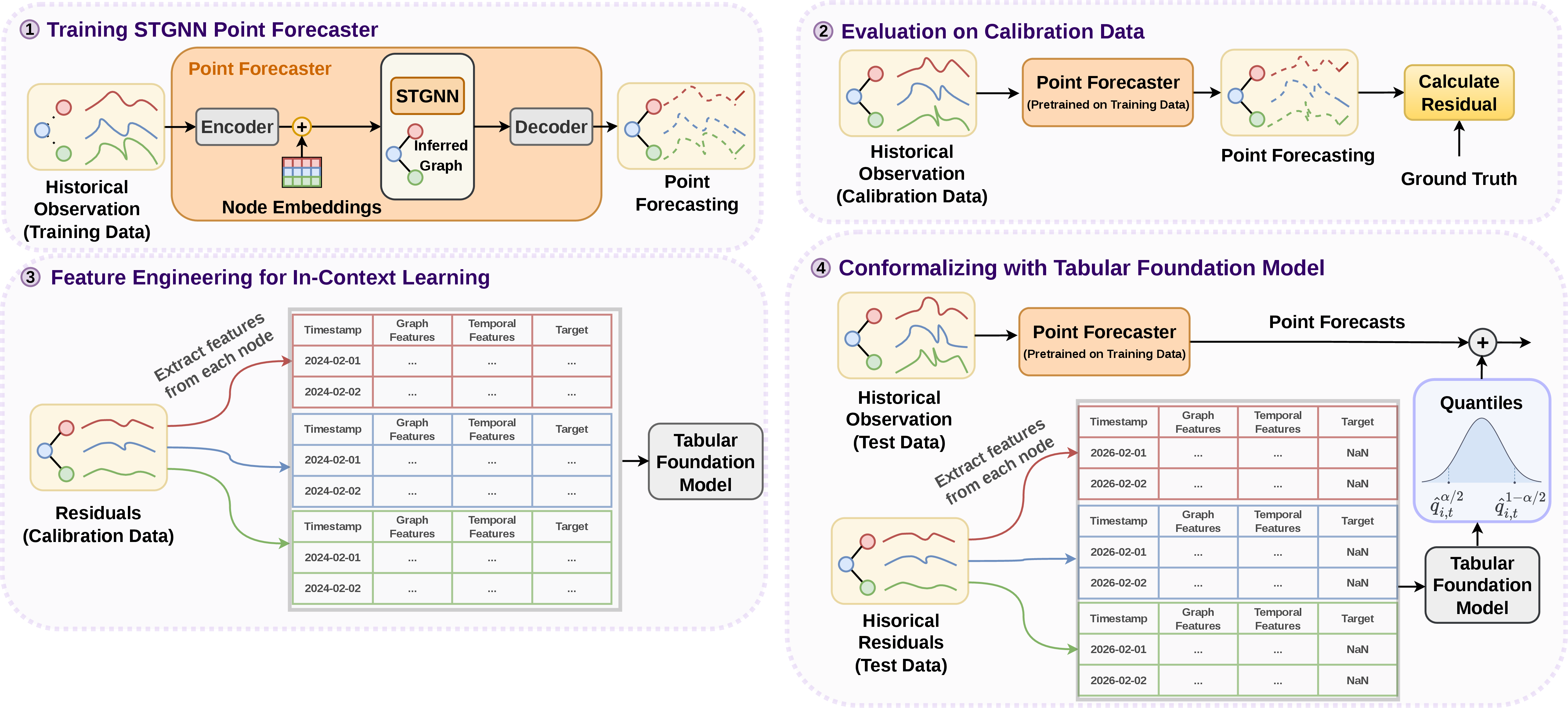
The STOIC framework decouples point forecasting from uncertainty quantification to address the structured residual behavior commonly observed in networked energy systems. Rather than relying on static calibration schemes, STOIC reformulates uncertainty estimation as an in-context learning problem by leveraging the zero-shot generalization capabilities of tabular FMs. The framework first employs an STGNN architecture to capture spatial-temporal dependencies and generate point forecasts. The resulting prediction residuals are then transformed into a structured tabular representation that captures both local neighborhood interactions and temporal dynamics. Finally, this contextual representation is used to construct adaptive PIs without requiring task-specific retraining. The following subsections detail the graph-based point forecasting architecture, the residual feature engineering procedure, and the in-context conformal calibration process. An overview of the full pipeline is illustrated in Fig. 1
3.1 Spatial-Temporal Architecture for Point Forecasting↩︎
The forecasting backbone of STOIC follows a shared spatial-temporal architecture for forecasting. For each node \(i\), the historical input sequence is first projected into a latent feature space through a shared encoder: \[\mathbf{h}^{(0)}_{i,t} = \mathrm{Encoder}(\mathbf{x}_{i,t-W:t-1}).\] The resulting node-level embeddings are stacked to form the global latent representation: \[\mathbf{H}^{(0)}_t = [\mathbf{h}^{(0)}_{1,t}, \dots, \mathbf{h}^{(0)}_{N,t}]^\top \in \mathbb{R}^{N \times d}.\] To incorporate node-specific characteristics, a learnable node embedding matrix \(\mathbf{V} \in \mathbb{R}^{N \times d}\) is added to the latent representation \(\mathbf{H}^{(0)}_t \leftarrow \mathbf{H}^{(0)}_t + \mathbf{V}\).
The resulting latent representations are subsequently processed by the STGNN backbone introduced in Section 2.3, which jointly models temporal dynamics and inter-node interactions: \[\mathbf{Z}_t = \mathrm{STGNN}(\mathbf{H}^{(0)}_t, \mathbf{A}).\] Finally, a shared decoder maps the latent node representations to the next-step forecasts: \[\hat{\mathbf{x}}_{t} = \mathrm{Decoder}(\mathbf{Z}_t),\] where \(\hat{\mathbf{x}}_{t} \in \mathbb{R}^{N}\) denotes the predicted observation vector at time \(t\). These point forecasts are subsequently used in the conformal calibration stage to construct uncertainty-aware prediction intervals.
3.2 Learning Sparse Graph from Data↩︎
In many real-world energy forecasting scenarios, the underlying interaction graph is not available a priori. Rather than assuming access to a predefined physical topology, STOIC learns the spatial dependencies directly from data. This design makes the framework applicable to systems where the true connectivity is unavailable, incomplete, or only partially reliable. Accordingly, the graph is treated as a latent object whose structure is learned jointly with the forecasting model. Given a collection of \(N\) nodes, we parameterize the pairwise connectivity through a learnable score matrix \(\mathbf{\Phi} \in \mathbb{R}^{N \times N}\), where each entry \(\phi_{ij}\) represents the affinity between nodes \(i\) and \(j\).
To construct a sparse neighborhood for each node, we sample \(K\) neighbors without replacement for each node \(i\). The probability of node \(j\) being selected is given by:
\[\pi_{ij} = \frac{\exp(\phi_{ij})}{\sum_{k=1}^{N} \exp(\phi_{ik})}, \quad j \in \{1, \dots, N\}\] The resulting sampled neighborhood defines the local connectivity set \(\mathcal{N}(i)\) for each node \(i\). The graph is learned end-to-end using the Gumbel-Top-\(K\) reparameterization trick [65] together with a straight-through gradient estimator [66]. This allows gradients to propagate through the discrete neighborhood selection process during training. As a result, STOIC can automatically discover sparse, task-specific spatial structures that are optimized for forecasting performance, even when the true system topology is unknown.
3.3 Spatial-Temporal Feature Engineering for In-Context Learning↩︎
After training the point forecasting backbone, STOIC is applied to the calibration split to obtain node-level prediction residuals. For every calibration time step \(t \in \mathcal{T}_{\mathrm{cal}}\), the residual vector is computed as: \[\mathbf{r}_t = \mathbf{x}_t - \hat{\mathbf{x}}_t.\] where \(\mathbf{x}_t\) denotes the observations and \(\hat{\mathbf{x}}_t\) represents the corresponding point forecasts produced by the STGNN backbone.
The objective of the subsequent feature engineering stage is to transform these residuals into structured tabular representations that can serve as contextual inputs for the tabular FM. Since tabular foundation models are designed to operate on fixed tabular inputs rather than graph-structured data, the spatial dependencies encoded in the underlying network cannot be directly processed in their native form. STOIC therefore converts the temporal and spatial residual structure into engineered tabular features that preserve informative neighborhood interactions while remaining compatible with the tabular FM architecture. Rather than treating calibration residuals as independent samples drawn from a stationary distribution, STOIC explicitly models their temporal and spatial structure. This design is motivated by empirical observations that forecasting errors in energy systems often exhibit strong temporal autocorrelation, heteroscedasticity, and cross-node dependence [67], [68]. Consequently, the uncertainty associated with a given node may depend not only on its own recent error history but also on the residual behavior of neighboring nodes.
To capture these dependencies, STOIC constructs feature vectors using only historical residual information available prior to the prediction time step, thereby preventing information leakage during calibration. For each target node \(i\), the resulting feature representation encodes multiple sources of contextual information derived from the calibration residual history. Specifically, the features are organized into three categories:
Temporal features, which capture the recent residual dynamics of the target node;
Graph-based features, which summarize residual patterns from neighboring nodes in the learned graph structure; and
Combined features, which integrate temporal and spatial context into a unified representation for in-context calibration.
These engineered representations provide the tabular FM with structured contextual information that enables adaptive estimation of the conditional residual distribution and, ultimately, the construction of context-aware prediction intervals.
3.3.1 Temporal Features↩︎
To capture the local temporal dynamics of forecasting errors at node \(i\), STOIC constructs features from the historical residual sequence \(\{r_{i,t-k} : k \ge 1\}\). These features are designed to summarize recent error behavior, including persistence, magnitude, and local variability, which are informative for estimating the conditional uncertainty at the current time step. Given a lag set \(\mathcal{P} = \{1, \dots, P\}\) and a collection of rolling window sizes \(\mathcal{W}\), compute summary statistics over past residuals. For each window \(w \in \mathcal{W}\), the rolling mean and rolling median are defined as: \[\mu^{(w)}_{i,t} = \frac{1}{w} \sum_{k=1}^{w} r_{i,t-k}, \quad \nu^{(w)}_{i,t} = \mathrm{median}\left(\{r_{i,t-k}\}_{k=1}^{w}\right).\] The temporal feature vector is then constructed as: \[\mathbf{f}^{\mathrm{temp}}_{i,t} = \big[ r_{i,t-p}, \; \mu^{(w)}_{i,t}, \; \nu^{(w)}_{i,t} \big]_{p \in \mathcal{P}, \; w \in \mathcal{W}}.\] These features provide the tabular FM with information about short-term residual trends and local uncertainty regimes. In particular, they enable the model to distinguish between stable forecasting periods and periods characterized by rapidly changing or highly variable residual behavior.
3.3.2 Graph-based Features↩︎
In addition to temporal patterns, STOIC explicitly incorporates information from neighboring nodes. Since tabular foundation models cannot directly process graph-structured inputs or perform message passing over adjacency relations, the spatial structure of the network must first be transformed into fixed-dimensional tabular representations. To achieve this, STOIC summarizes neighborhood residual behavior through permutation-invariant aggregation operators, effectively translating graph-level information into a format compatible with tabular FMs.
This design mirrors the message-passing mechanism used in graph neural networks, where node representations are updated through aggregation of information from local neighborhoods. Following the same principle, STOIC constructs graph-based features that summarize neighboring residual dynamics while remaining invariant to the ordering of neighboring nodes.
Let \(\mathcal{N}(i)\) denote the set of neighbors of node \(i\) in the learned or predefined adjacency structure \(\mathbf{A}\). For each lag \(p \in \mathcal{P}\) and aggregation operator \(g(\cdot)\), we compute: \[a^{g,p}_{i,t} = g\left(\left\{ r_{j,t-p} : j \in \mathcal{N}(i) \right\}\right),\] where \(g(\cdot)\) is a permutation-invariant operator such as the mean, median, minimum, or maximum.
The resulting graph-based feature vector is defined as: \[\mathbf{f}^{\mathrm{graph}}_{i,t} = \big[ a^{\mathrm{mean},p}_{i,t}, a^{\mathrm{median},p}_{i,t}, a^{\mathrm{min},p}_{i,t}, a^{\mathrm{max},p}_{i,t} \big]_{p=1}^{P}.\]
These features encode the local spatial context of node \(i\) by summarizing how neighboring nodes behaved in the recent past. This is particularly important in energy systems, where nearby or functionally related locations often exhibit correlated demand patterns, shared environmental influences, or common system-level disturbances. Consequently, residual behavior observed at neighboring nodes can provide informative signals for estimating uncertainty at the target nodes.
3.3.3 Combined Feature Representation↩︎
The final contextual representation for node \(i\) at calibration time \(t\) is obtained by concatenating the temporal and graph-based feature components: \[\mathbf{f}_{i,t} = \left[ \mathbf{f}^{\mathrm{temp}}_{i,t}, \mathbf{f}^{\mathrm{graph}}_{i,t} \right].\]
This concatenated vector defines a structured tabular sample whose target variable is the corresponding calibration residual \(r_{i,t}\). In STOIC, these feature-target pairs constitute the contextual dataset provided to the tabular FM used for in-context calibration. Feature extraction is performed independently for each node, resulting in a collection of node-specific tabular datasets that encode both temporal residual dynamics and spatial neighborhood information. This representation preserves local temporal history, incorporates spatial context through permutation-invariant neighbor aggregation, and avoids leakage by relying only on past residuals. Together, these features provide the foundation for the next stage, where the tabular FM (e.g., TabPFN) is used to infer calibrated uncertainty estimates.
3.4 Conformalizing with Tabular Foundation Model↩︎
Given the engineered feature representations, STOIC performs uncertainty estimation by formulating residual modeling as a tabular regression problem. Rather than relying on fixed empirical residual quantiles as in standard CP, STOIC leverages a tabular FM to learn the conditional residual distribution in an in-context manner. For each node \(i\), we construct a dataset consisting of feature-residual pairs \(\{(\mathbf{f}_{i,t}, r_{i,t})\}_{t \in \mathcal{T}_{\mathrm{cal}}}\), where \(\mathbf{f}_{i,t}\) denotes the engineered contextual feature vector and \(r_{i,t}\) is the corresponding calibration residual. A pretrained tabular FM is then applied in-context to map features, constructed from the history of past residuals and their spatial context, to residual values:
\[r_{i,t} = h_\psi(\mathbf{f}_{i,t}),\] where \(h_\psi(\cdot)\) denotes the tabular FM parameterized by \(\psi\).
At inference time, given a new input window \(\mathbf{X}_{t-W:t-1}\) from the test set, the STGNN backbone first produces the point forecast \(\hat{x}_{i,t}\). The corresponding contextual feature vector \(\mathbf{f}_{i,t}\) is then constructed using the same feature engineering procedure applied during calibration. Conditioned on this representation, the tabular FM predicts quantiles of the residual distribution: \[\hat{q}_{i,t}^{\alpha} = h_\psi^{(\alpha)}(\mathbf{f}_{i,t}),\] where \(h_\psi^{(\alpha)}(\cdot)\) denotes the predicted \(\alpha\)-quantile of the conditional residual distribution. The PI is subsequently obtained by shifting the predicted residual quantiles around the point forecast: \[C_{i,t}^\alpha = \left[ \hat{x}_{i,t} + \hat{q}_{i,t}^{\alpha/2}, \; \hat{x}_{i,t} + \hat{q}_{i,t}^{1-\alpha/2} \right].\]
This formulation can be interpreted as a learned, feature‑conditional generalization of CP. While classical conformal methods use global residual quantiles, STOIC adapts the interval width based on the local temporal and spatial context encoded in \(\mathbf{f}_{i,t}\). As a result, the method produces heteroscedastic and context‑aware PIs. Unlike classical conformal approaches that rely on exchangeability, STOIC explicitly conditions on structured residual context, enabling it to capture regime‑dependent uncertainty patterns that are inaccessible to global calibration. Importantly, this procedure does not require retraining the forecasting backbone. The tabular FM operates purely on residual features, enabling a modular pipeline where forecasting and uncertainty quantification are decoupled. This also allows leveraging the zero‑shot generalization capabilities of modern tabular models to perform calibration with limited data.
Remark 1 (Distinction with quantile regression). We emphasize that STOIC is fundamentally different from conventional quantile regression approaches. Classical quantile regression directly models conditional quantiles of the target variable and therefore typically requires either multiple independently trained models or dedicated output heads for different quantile levels. As a result, uncertainty estimation becomes tightly coupled to the forecasting architecture and often requires extensive task-specific retraining, hyperparameter tuning, and calibration. In contrast, STOIC performs uncertainty estimation post hoc on the residuals of an arbitrary pretrained point forecaster. The framework transforms spatial-temporal residual structure into a tabular contextual representation and uses a pretrained tabular FM to infer conditional residual quantiles in-context. This design yields several important advantages. First, STOIC is fully modular and can be applied to any forecasting architecture without altering or retraining the underlying predictor. Second, uncertainty estimation is conditioned on structured residual context rather than learned jointly with the forecasting objective, enabling adaptive interval construction even when the forecasting model itself was not optimized for probabilistic prediction. Third, by leveraging pretrained tabular FMs, STOIC inherits strong zero‑shot generalization and the ability to operate effectively with limited calibration data, which are difficult to obtain with standard quantile regression pipelines.
Conceptually, STOIC remains aligned with the conformal inference perspective, where uncertainty is calibrated through residual behavior rather than direct target quantile prediction. However, STOIC extends this principle beyond global calibration by introducing feature-conditional residual modeling tailored to graph-structured spatial-temporal systems.
Remark 2 (Expressive capacity and motivation for the feature representation). Let \(\mathbf{f}_{i,t}\) denote the engineered feature vector constructed from the recent residual history of node \(i\) together with aggregated permutation‑invariant statistics of neighboring residuals. Any continuous function defined on a compact domain that depends on these quantities can, in principle, be approximated arbitrarily well by a universal approximator operating on \(\mathbf{f}_{i,t}\). Consequently, an idealized model conditioned on the engineered features can emulate a restricted class of one‑hop message‑passing functions whose neighborhood interactions are fully characterized by the selected aggregation operators.
Furthermore, if the true conditional distribution of the residual \(r_{i,t}\) depends on the neighbors’ past residuals solely through these permutation-invariant statistics, then \(\mathbf{f}_{i,t}\) captures all the conditioning information necessary to determine the true conditional quantiles. Even when this assumption is only partially satisfied, the selected aggregates provide a compact, informative summary sufficient for the tabular model to estimate the conditional quantiles. In practice, the fixed pretrained model \(h_\psi(\cdot)\) produces a non-linear empirical approximation, the fidelity of which is governed by the model’s inherent capacity and the relevance of its pretraining distribution.
Proposition 1 (Asymptotic conditional coverage under an oracle estimator). Let \(r_{i,t}=x_{i,t}-\hat{x}_{i,t}\) and let \(F_{r|f}(\cdot\mid\mathbf{f}_{i,t})\) be its true conditional cumulative distribution function. For a target level \(\beta\in(0,1)\), denote by \(q^{\beta}(\mathbf{f}_{i,t})\) the true conditional quantile satisfying \(\mathbb{P}\bigl(r_{i,t}\le q^{\beta}(\mathbf{f}_{i,t})\mid\mathbf{f}_{i,t}\bigr)=\beta\). Assume that:
\(F_{r|f}(\cdot\mid\mathbf{f}_{i,t})\) is continuous at \(q^{\alpha/2}(\mathbf{f}_{i,t})\) and \(q^{1-\alpha/2}(\mathbf{f}_{i,t})\);
an oracle* estimator provides consistent estimates of both conditional quantiles: \[\hat{q}^{\alpha/2}(\mathbf{f}_{i,t})\xrightarrow{p} q^{\alpha/2}(\mathbf{f}_{i,t}), \quad \hat{q}^{1-\alpha/2}(\mathbf{f}_{i,t})\xrightarrow{p} q^{1-\alpha/2}(\mathbf{f}_{i,t}),\] as the number of calibration samples \(n\to\infty\).*
Then the prediction interval \[C_{i,t}^{\alpha}= \Bigl[\,\hat{x}_{i,t}+\hat{q}^{\alpha/2}(\mathbf{f}_{i,t}),\; \hat{x}_{i,t}+\hat{q}^{1-\alpha/2}(\mathbf{f}_{i,t})\,\Bigr]\] achieves asymptotic conditional coverage: \[\mathbb{P}\bigl(x_{i,t}\in C_{i,t}^{\alpha}\mid\mathbf{f}_{i,t}\bigr) \;\xrightarrow{p}\; 1-\alpha .\]
Proof. Because \(x_{i,t}=\hat{x}_{i,t}+r_{i,t}\), the event \(x_{i,t}\in C_{i,t}^{\alpha}\) is equivalent to \[\hat{q}^{\alpha/2}(\mathbf{f}_{i,t}) \le r_{i,t} \le \hat{q}^{1-\alpha/2}(\mathbf{f}_{i,t}).\] It therefore suffices to establish coverage for the residual interval.
\[\mathbb{P}\bigl(r_{i,t}\le q^{\alpha/2}(\mathbf{f}_{i,t})\mid\mathbf{f}_{i,t}\bigr) = \alpha/2,\] \[\mathbb{P}\bigl(r_{i,t}\le q^{1-\alpha/2}(\mathbf{f}_{i,t})\mid\mathbf{f}_{i,t}\bigr) = 1-\alpha/2 .\]
Under the oracle assumption, the estimated quantiles are consistent: \[\begin{align} \hat{q}^{\alpha/2}(\mathbf{f}_{i,t}) &\xrightarrow{p} q^{\alpha/2}(\mathbf{f}_{i,t}),\\ \hat{q}^{1-\alpha/2}(\mathbf{f}_{i,t}) &\xrightarrow{p} q^{1-\alpha/2}(\mathbf{f}_{i,t}). \end{align}\]
Since \(F_{r|f}(\cdot\mid\mathbf{f}_{i,t})\) is continuous at the true quantiles, the Continuous Mapping Theorem yields \[F_{r|f}\bigl(\hat{q}^{\alpha/2}(\mathbf{f}_{i,t})\mid\mathbf{f}_{i,t}\bigr) \xrightarrow{p} F_{r|f}\bigl(q^{\alpha/2}(\mathbf{f}_{i,t})\mid\mathbf{f}_{i,t}\bigr) = \alpha/2,\] \[F_{r|f}\bigl(\hat{q}^{1-\alpha/2}(\mathbf{f}_{i,t})\mid\mathbf{f}_{i,t}\bigr) \xrightarrow{p} F_{r|f}\bigl(q^{1-\alpha/2}(\mathbf{f}_{i,t})\mid\mathbf{f}_{i,t}\bigr) = 1-\alpha/2 .\]
Therefore, \[\begin{align} &\mathbb{P}\bigl( \hat{q}^{\alpha/2}(\mathbf{f}_{i,t}) \le r_{i,t} \le \hat{q}^{1-\alpha/2}(\mathbf{f}_{i,t}) \mid \mathbf{f}_{i,t} \bigr) = F_{r|f}\bigl(\hat{q}^{1-\alpha/2}(\mathbf{f}_{i,t})\mid\mathbf{f}_{i,t}\bigr) - F_{r|f}\bigl(\hat{q}^{\alpha/2}(\mathbf{f}_{i,t})\mid\mathbf{f}_{i,t}\bigr) \\ &\xrightarrow{p} (1-\alpha/2) - \alpha/2 = 1-\alpha . \end{align}\]
Shifting the interval by the point forecast \(\hat{x}_{i,t}\) preserves the coverage probability, so the same limit holds for \(x_{i,t}\). ◻
Remark 3 (On the oracle assumption and the choice of TabPFN). Proposition 1 establishes an asymptotic oracle result under the assumption that the conditional residual quantiles are estimated consistently. Existing approaches [48]–[50] satisfy this requirement using quantile random forests trained from scratch on the calibration set, which are provably consistent under certain assumptions [48], [69]. In contrast, TabPFN is a prior-fitted network [58] designed to approximate Bayesian inference. Because it relies on a synthetic prior, it lacks theoretical guarantees for consistently estimating arbitrary conditional distributions [70]. Despite this theoretical gap, TabPFN introduces practical advantages that make it highly effective for the STOIC framework. First, its in-context learning capabilities enable zero-shot calibration across diverse nodes without the need for task-specific retraining. Second, its strong pre-trained inductive biases successfully capture complex residual patterns that would otherwise require prohibitively large calibration datasets for methods like random forests. Finally, TabPFN’s in‑context learning capability makes it straightforward to share one pretrained model across all nodes, simplifying deployment compared to methods that require per‑node training
Overall, while TabPFN does not strictly satisfy the oracle assumption, it acts as a powerful approximation. Its coverage deviation is bounded by the total variation distance (as detailed in Remark 4), and its empirical performance consistently outperforms conventional alternatives.
Remark 4 (Coverage bound without the oracle assumption).
Proposition 1 assumes a consistent estimator of the conditional quantiles. In practice, the pretrained tabular foundation model only provides an approximation to the true conditional residual distribution. The following argument gives a qualitative interpretation of how approximation error affects coverage. For a fixed calibration set, let \(\hat{q}^{\alpha/2}(\mathbf{f}_{i,t}),\hat{q}^{1-\alpha/2}(\mathbf{f}_{i,t})\) denote the quantiles predicted by the tabular FM. Define a distribution \(P_{\psi}^c\) whose \(\alpha/2\) and \(1-\alpha/2\) quantiles equal exactly these values (e.g., a continuous uniform distribution between them with \(\alpha/2\) point masses at the boundaries). By construction, \[\mathbb{P}_{P_{\psi}^c}\!\bigl( r_{i,t} \in [\hat{q}^{\alpha/2},\, \hat{q}^{1-\alpha/2}] \bigr) = 1-\alpha .\]
Let \(P_{t}^c\) be the true conditional residual distribution, and let \(B = \bigl\{ r_{i,t} \in [\hat{q}^{\alpha/2},\,\hat{q}^{1-\alpha/2}] \bigr\}\). By the definition of total variation distance, \[\bigl|\mathbb{P}_{P_{t}^c}(B) - \mathbb{P}_{P_{\psi}^c}(B)\bigr| \le \mathrm{TV}(P_{t}^c,\,P_{\psi}^c) .\] Consequently, \[\mathbb{P}_{P_{t}^c}(B) \;\ge\; 1-\alpha - \mathrm{TV}\bigl(P_{t}^c,\,P_{\psi}^c\bigr),\] where \(\mathrm{TV}(\cdot,\cdot)\) denotes the total variation distance [51]. This is a lower limit: actual coverage can be higher than \(1-\alpha\) if the interval is conservatively wide, even when \(\mathrm{TV}>0\). The bound is not computable in practice, but it gives a qualitative interpretation: the better \(P_{\psi}^c\) approximates the true conditional residual distribution, the smaller the potential coverage gap.
4 Experimental Setup↩︎
4.1 Datasets↩︎
We evaluate STOIC on a diverse collection of synthetic and real-world datasets, including controlled simulations and large-scale energy systems. Across all datasets, we define the forecasting task as predicting one-day-ahead demand from the previous seven days of observations. To facilitate model training and evaluation, each dataset is partitioned chronologically into training, calibration, and testing sets, following a 70%, 15%, and 15% split, respectively. The training split is used exclusively for learning the point forecasting backbone, while the calibration split is reserved for residual-based uncertainty estimation. Furthermore, for training point forecaster, all data are standardized by subtracting the mean and dividing by the standard deviation, with statistics computed solely from the training set to prevent data leakage.
Simulated Control Signals (SCS): To evaluate STOIC under controlled conditions with known ground-truth dynamics, we generate a synthetic dataset driven by two latent control signals, \(u_1(t)\) and \(u_2(t)\), modeled as sinusoids: \[u_1(t) = \sin(2\pi \cdot 1.2t + 0.2),\] \[u_2(t) = 0.8 \sin(2\pi \cdot 0.45t - 0.5).\] We define 10 measurement nodes (\(y_1, \dots, y_{10}\)) where each node is a non-linear combination of these latent drivers and a low-frequency temporal drift. Specifically, each measurement \(y_i\) is generated as: \[y_i(t) = f_i(u_1(t), u_2(t)) + s_i(t) + \epsilon_i,\] where \(f_i(\cdot)\) represents node-specific interactions, \(s_i(t)\) represents a slow-moving seasonal component, and \(\epsilon_i \sim \mathcal{N}(0, \sigma^2)\) is additive white Gaussian noise. The noise variance \(\sigma^2\) is dynamically adjusted for each node to maintain a strict Signal-to-Noise Ratio (SNR) of 45 dB. In total, we generate 3650 daily time steps for each measurement node.
Synthetic District Heating (SDH): We simulate a district heating network comprising 100 buildings (spatial nodes) with heterogeneous thermal characteristics using the demandlib library2. The simulated network comprises 60% single-family houses, 30% multi-family houses, and 10% commercial buildings to reflect realistic variability in building usage and consumption behavior. To introduce
heterogeneity across the network, each building is assigned a unique seasonal demand profile with varying peak intensities and transition dynamics. In addition, we incorporate realistic consumption dynamics by including auto‑correlated fluctuations
(modeled as a multiplicative first‑order autoregressive (AR(1)) noise with per‑building autocorrelation coefficients uniformly sampled from [0.75, 0.85] and relative magnitudes between 2.5% and 5%) as well as weekend‑specific behavioral variations. The
simulation spans the period from 2010 to 2019 at daily resolution, resulting in 3652 observations per building. This dataset provides a controlled yet realistic environment for evaluating uncertainty estimation under heterogeneous spatial-temporal demand
patterns.
District Heating (EWZ): This dataset consists of daily real-world district heating consumption measurements provided by Elektrizitätswerk der Stadt Zürich (EWZ), a Swiss energy utility company. The dataset contains heat demand observations from 48 buildings (spatial nodes) located in Switzerland from April 1, 2016, to October 31, 2025, resulting in 3501 daily observations per node. Measurements are in MWh and reflect the complexity of an operational district heating network, including heterogeneous consumption behavior, irregular occupancy patterns, seasonal demand fluctuations, and measurement noise. As a result, the dataset provides a realistic and challenging benchmark for evaluating uncertainty quantification methods in physical energy distribution systems.
Electricity Consumption Load (ECL): The ECL dataset3 comprises electricity consumption measurements collected from clients in Portugal at 15-minute resolution. Although the original monitoring network is larger, several clients were excluded because their meters were not installed at the start of the observation period or contained significant gaps. After filtering for continuous measurements, 40 clients were retained and treated as spatial nodes. To ensure consistency with the other datasets and reduce high-frequency consumption noise, the original power measurements (kW) were converted to energy consumption (kWh) and aggregated to daily totals. We consider the period from January 1, 2011 to December 31, 2014, resulting in 1461 daily observations per client. The dataset captures heterogeneous electricity demand patterns across consumers and provides a realistic benchmark for evaluating spatial-temporal forecasting and uncertainty quantification methods under diverse consumption behaviors.
Smart Meter Aggregates (CKW): This dataset, provided by Centralschweizerische Kraftwerke AG (CKW)4 consists of smart meter electricity consumption measurements aggregated at the postal code level to preserve consumer privacy. Out of the 116 municipalities originally available, we retain 93 that do not have significant missing values. We consider these 93 municipality-level spatial nodes over the period from December 31, 2020, to February 5, 2026. Large industrial consumers are excluded in order to focus on residential consumption dynamics. Original measurements are recorded at 15-minute resolution and aggregated to daily energy consumption values (kWh) to align with the temporal granularity of the other datasets. This results in 1863 daily observations for each spatial node. The dataset captures heterogeneous residential demand patterns across municipalities, providing a realistic large-scale benchmark for spatial-temporal uncertainty quantification.
4.2 Baselines↩︎
We compare STOIC against a diverse set of CP baselines spanning global, temporal, and spatially extended approaches. Split Conformal Prediction (SCP) [61] provides valid marginal coverage but produces uniform prediction intervals by disregarding spatial and temporal heterogeneity. To account for temporal non-stationarity, Adaptive Conformal Inference (ACI) [47] and Sequential Predictive Conformal Inference (SPCI) [48] dynamically adapt interval widths based on recent coverage errors and historical residuals, respectively. However, both methods model each time series independently and therefore fail to capture dependencies across nodes. To incorporate spatial structure, Localized Spatial Conformal Prediction (LSCP) [49] and Spatial-Temporal Conformal Prediction (STCP) [50] introduce spatially-aware calibration mechanisms. In contrast, STOIC employs a tabular FM to learn feature-conditional residual distributions jointly across space and time, producing fully adaptive and context-aware PIs without task-specific retraining. To ensure a fair comparison, all conformal methods utilize the same point forecasting backbone described in Section 3, and all evaluations are conducted at a target confidence level of \(1-\alpha = 0.90\).
4.3 Performance Metrics↩︎
We evaluate the quality of the predicted intervals using standard metrics that assess both calibration and sharpness. Given a PI \(C_{i,t}^\alpha = [\ell_{i,t}^\alpha, u_{i,t}^\alpha]\) at confidence level \(1-\alpha\) and the corresponding ground-truth value \(x_{i,t}\), we consider the following metrics.
Prediction Interval Width (PI-Width): PI-Width measures the sharpness of the interval and is defined as: \[\text{(PI-Width)}_{i,t} = u_{i,t}^\alpha - \ell_{i,t}^\alpha.\] Lower values indicate tighter intervals.
Coverage: Coverage measures the proportion of observations contained within the predicted intervals: \[\text{Coverage} = \mathbb{E}\left[ \mathbb{I}\left(x_{i,t} \in C_{i,t}^\alpha \right) \right],\] where \(\mathbb{I}(\cdot)\) is the indicator function. Ideally, the empirical coverage should closely match the target confidence level.
Winkler Score: The Winkler score [71] jointly evaluates PI width and calibration by penalizing PIs that fail to cover the true value: \[\text{Winkler Score}= \begin{cases} u_{i,t}^\alpha - \ell_{i,t}^\alpha, & \text{if } x_{i,t} \in C_{i,t}^\alpha, \\ (u_{i,t}^\alpha - \ell_{i,t}^\alpha) + \frac{2}{\alpha}(\ell_{i,t}^\alpha - x_{i,t}), & \text{if } x_{i,t} < \ell_{i,t}^\alpha, \\ (u_{i,t}^\alpha - \ell_{i,t}^\alpha) + \frac{2}{\alpha}(x_{i,t} - u_{i,t}^\alpha), & \text{if } x_{i,t} > u_{i,t}^\alpha. \end{cases}\] The Winkler score rewards narrow prediction intervals while imposing increasingly large penalties for prediction failures. All metrics are averaged across all nodes and time steps to provide a global assessment of uncertainty quantification performance.
5 Results and Discussion↩︎
5.1 Quantitative Results↩︎
This section presents the empirical evaluation of STOIC against several CP baselines across all datasets. All experiments were conducted at a target confidence level of \(90\%\).
The results on the SCS dataset, detailed in Table 1, highlight substantial differences in calibration performance across methods. Notably, only STCP and STOIC achieve empirical coverage at or above the nominal 90% target, whereas all remaining baselines suffer from systematic under-coverage, with coverage values around 88%. This finding is particularly important, as under-coverage indicates a violation of the intended statistical reliability guarantees. Furthermore, methods such as SCP and ACI attempt to improve coverage by producing wider prediction intervals, yet still fail to reach the target coverage level, resulting in an unfavorable trade-off between reliability and sharpness. In contrast, STOIC achieves a PI-Width of 0.0309, which is approximately 20% narrower than the strongest temporal baseline, SPCI, while simultaneously maintaining valid coverage. This advantage is further reflected in the Winkler Score, where STOIC achieves the lowest value among all compared methods. These results demonstrate that STOIC is uniquely able to combine accurate calibration with highly informative prediction intervals, whereas competing approaches either sacrifice coverage guarantees or require substantially wider intervals to achieve comparable performance.
| Method | Coverage (%) | PI-Width ↓ | Winkler Score ↓ |
|---|---|---|---|
| SCP | 88.13 | 0.0490 | 0.0826 |
| SPCI | 88.39 | 0.0387 | 0.0588 |
| ACI | 88.83 | 0.0517 | 0.0791 |
| LSCP | 88.01 | 0.0444 | 0.0691 |
| STCP | 90.90 | 0.0388 | 0.0549 |
| STOIC | 91.57 | 0.0309 | 0.0435 |
The results on the SDH dataset, shown in Table 2, show a different behavior compared to SCS. All methods achieve empirical coverage at or above the nominal 90% level, indicating that calibration is less challenging on this dataset. As a result, the comparison is driven primarily by interval efficiency rather than coverage. Under these conditions, STOIC produces the narrowest prediction intervals among the compared methods while maintaining the required coverage guarantees. This demonstrates that STOIC can translate equivalent calibration performance into substantially more precise uncertainty estimates, thereby providing a more favorable balance between reliability and informativeness.
| Method | Coverage (%) | PI-Width ↓ | Winkler Score ↓ |
|---|---|---|---|
| SCP | 90.78 | 0.0082 | 0.0126 |
| SPCI | 90.04 | 0.0077 | 0.0111 |
| ACI | 90.63 | 0.0082 | 0.0126 |
| LSCP | 90.12 | 0.0077 | 0.0114 |
| STCP | 90.59 | 0.0075 | 0.0104 |
| STOIC | 91.05 | 0.0067 | 0.0093 |
For the real-world EWZ dataset, the results in Table 3 further demonstrate the effectiveness of STOIC. The method achieves an empirical coverage of 90.15%, closely matching the nominal target and resulting in the smallest coverage gap among the compared approaches. At the same time, STOIC produces substantially narrower prediction intervals than LSCP, despite the latter explicitly leveraging spatial neighborhoods (PI-Width: 0.4594 vs. 0.3947). The resulting Winkler Score of 0.6478 is the lowest across all compared methods, demonstrating that STOIC consistently achieves a more favorable balance between calibration accuracy and interval sharpness on a real-world utility network dataset.
| Method | Coverage (%) | PI-Width ↓ | Winkler Score ↓ |
|---|---|---|---|
| SCP | 92.56 | 0.4391 | 0.6995 |
| SPCI | 90.88 | 0.4154 | 0.6941 |
| ACI | 92.12 | 0.4266 | 0.6973 |
| LSCP | 90.90 | 0.4594 | 0.7219 |
| STCP | 91.28 | 0.4335 | 0.7028 |
| STOIC | 90.15 | 0.3947 | 0.6478 |
The ECL evaluation, summarized in Table 4, shows that STOIC and STCP are the only methods that achieve coverage above the nominal 90% level (90.52% and 90.53%, respectively), whereas SPCI and LSCP exhibit under-coverage. Although both STOIC and STCP provide valid coverage, STOIC achieves a substantially lower Winkler Score (1674.85 vs. for STCP), indicating more efficient uncertainty quantification. While LSCP produces the narrowest prediction intervals, it fails to meet the target coverage level, demonstrating that increased sharpness comes at the expense of calibration. Overall, STOIC is the only method that simultaneously achieves near-nominal coverage and the best overall interval quality, as reflected by its superior Winkler Score.
| Method | Coverage (%) | PI-Width ↓ | Winkler Score ↓ |
|---|---|---|---|
| SCP | 93.65 | 1288.53 | 1874.88 |
| SPCI | 89.44 | 1199.82 | 1929.06 |
| ACI | 93.43 | 1278.77 | 1867.85 |
| LSCP | 89.27 | 1137.70 | 1783.94 |
| STCP | 90.53 | 1193.72 | 1813.12 |
| STOIC | 90.52 | 1168.54 | 1674.85 |
Finally, the results on the CKW dataset in Table 5 highlight a clear trade-off between coverage and interval efficiency. Only SCP, ACI, and STOIC achieve coverage at or above the nominal 90% level, whereas SPCI, LSCP, and STCP exhibit under-coverage. Although STCP produces the narrowest prediction intervals, this gain is achieved at the expense of violating the desired coverage guarantee. In contrast, STOIC maintains valid coverage while producing intervals that remain competitive in width. This advantage is reflected in the lowest Winkler Score among all compared methods, indicating that STOIC is able to preserve calibration without resorting to overly conservative uncertainty estimates. These results further demonstrate that STOIC delivers the highest-quality prediction intervals by combining reliable coverage with efficient interval widths.
| Method | Coverage (%) | PI-Width ↓ | Winkler Score ↓ |
|---|---|---|---|
| SCP | 91.80 | 3001.00 | 3916.29 |
| SPCI | 88.97 | 2131.12 | 3067.55 |
| ACI | 91.25 | 2937.59 | 3911.71 |
| LSCP | 89.06 | 2156.72 | 3132.60 |
| STCP | 89.77 | 2123.03 | 2936.83 |
| STOIC | 90.89 | 2156.48 | 2927.36 |
5.2 Qualitative Results↩︎
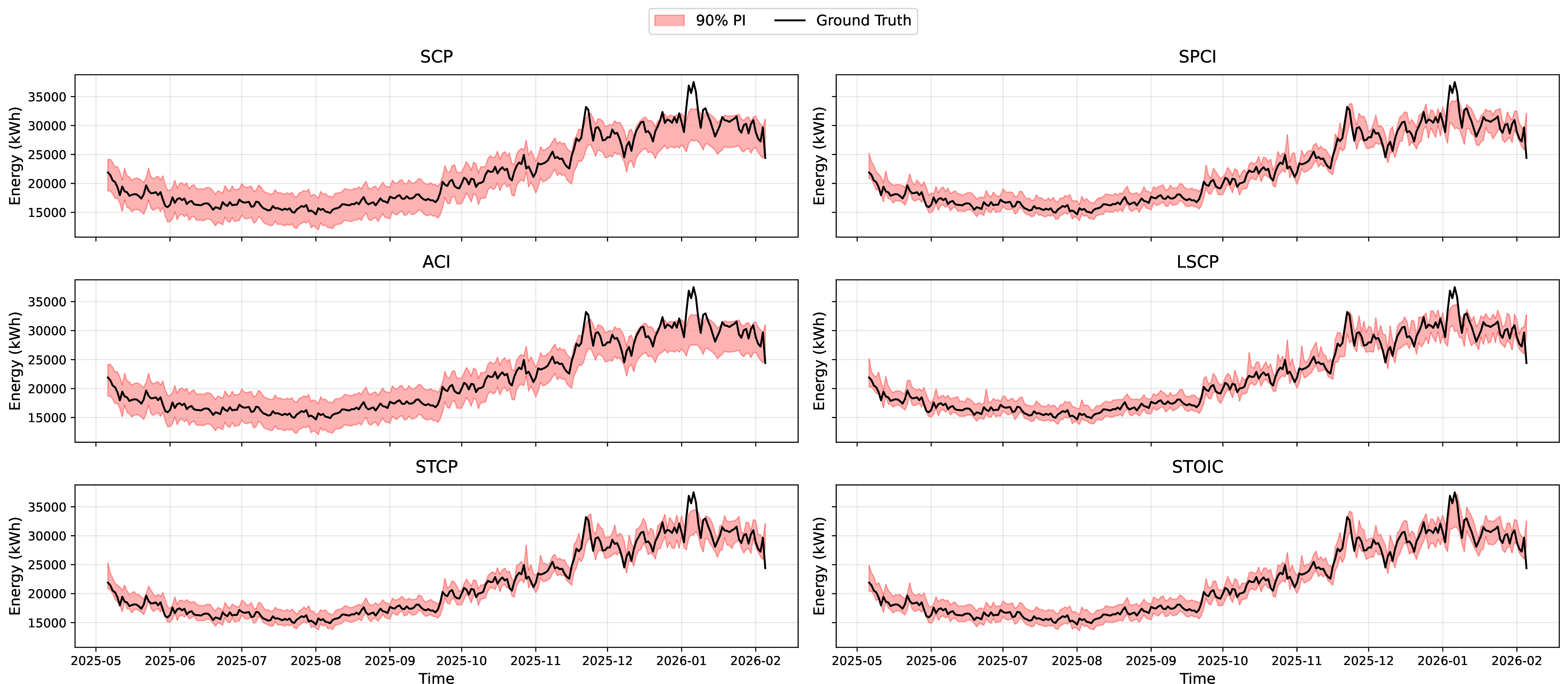
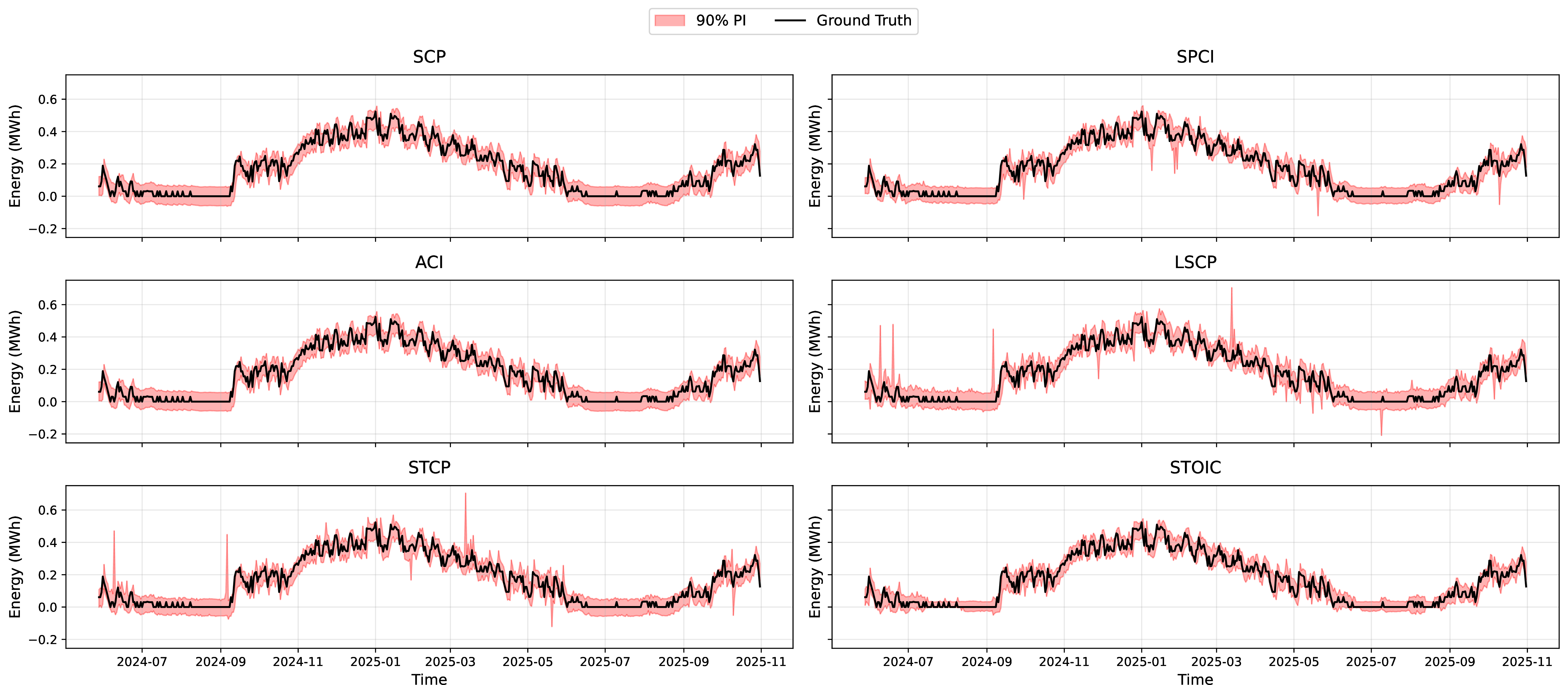
The qualitative analysis is conducted on the CKW and EWZ datasets because they represent two distinct forecasting settings. While CKW exhibits substantial temporal variability in electricity demand, EWZ is characterized by strong seasonality and noisier demand patterns. This allows the behavior of the prediction intervals to be examined under different sources of uncertainty.
Figure 2 provides a qualitative comparison of the 90% PIs for the CKW dataset, spanning from May 2025 to February 2026. While all methods successfully capture the broad upward trend in energy consumption during the winter months, there are distinct differences in interval efficiency. Standard methods like SCP and ACI exhibit relatively static or overly broad intervals that do not tightly track the daily volatility of the aggregated load. In contrast, STOIC produces substantially more adaptive intervals, remaining narrow during stable periods while expanding only when the underlying signal exhibits increased variability or rapid fluctuations. This behavior indicates that uncertainty is allocated where it is needed rather than uniformly across time. The resulting intervals more closely follow the local uncertainty structure of the data, providing sharper and more informative uncertainty estimates. This visual evidence supports the quantitative findings that STOIC achieves superior interval efficiency while maintaining reliable coverage in aggregated smart meter networks. The visualization for the EWZ dataset in Figure 3 highlights how different methods respond to the extreme seasonality and noise typical of heat demand. A key observation in the LSCP and STCP plots is the presence of sharp, vertical spikes in the PIs during the early and mid-2025 periods. These spikes indicate that these methods are highly sensitive to localized spatial outliers, sometimes leading to excessively conservative (wide) intervals that may be less useful for practical demand forecasting and operational planning. Such abrupt expansions suggest that uncertainty estimates are being driven by isolated observations rather than by the overall uncertainty structure of the system. STOIC, however, maintains a much smoother and more consistent adaptive envelope. By conditioning on a broader set of features through its Tabular FM, STOIC avoids overreacting to individual noisy data points while still ensuring the 90% PI encompasses the ground truth throughout the transition from high-demand winter months to low-demand summer periods. Importantly, STOIC achieves this stability without sacrificing responsiveness to genuine changes in demand patterns, resulting in uncertainty estimates that are both more robust and more informative for operational decision-making.
5.3 Comparison with a Time-Series Foundation Model↩︎
Recent advances in time-series foundation models have established large-scale pretrained forecasting models as a strong benchmark for both point forecasting and uncertainty quantification. Comparing STOIC against such models is therefore important for assessing the value of its spatial-temporal forecasting and conformal calibration pipeline relative to a general-purpose foundation model trained on a broad collection of time-series data. To address this question, we compare STOIC against TimesFM [72]. , one of the most widely adopted foundation models for time-series forecasting. While many foundation models focus exclusively on point forecasting and do not provide calibrated uncertainty estimates, TimesFM is particularly suitable for this comparison because its latest release (version 2.5) supports probabilistic forecasting. TimesFM is a 200M-parameter decoder-only transformer pretrained on a large corpus of real-world and synthetic time series. Comparing against TimesFM therefore provides a particularly strong baseline and allows us to assess whether the spatial-temporal modeling and conformal calibration components of STOIC continue to provide benefits beyond large-scale pretraining.
The pretrained model returns point forecasts along with deciles, specifically the quantiles at 10%, 20%, …, 90% levels. To ensure a fair comparison, both methods are therefore evaluated at a target coverage of 80%, corresponding to the 0.1 and 0.9 quantiles. We perform the comparison on the two real-world datasets, EWZ and CKW, which represent different demand forecasting settings and are not part of the publicly documented TimesFM pretraining corpus. This setting enables a fair zero-shot evaluation and avoids potential concerns regarding data leakage. For STOIC, only the conformal calibration stage is adjusted to the 80% target level; the forecasting backbone and learned representations remain unchanged. The resulting comparison therefore isolates the relative quality of the uncertainty estimates produced by a large-scale foundation model and a dedicated spatial-temporal conformal prediction framework. The results are summarized in Table 6.
| Dataset | Method | Coverage (%) | PI-Width \(\downarrow\) | Winkler Score \(\downarrow\) |
|---|---|---|---|---|
| EWZ | TimesFM | 73.47 | 0.2748 | 0.7798 |
| STOIC | 80.40 | 0.2954 | 0.4830 | |
| CKW | TimesFM | 71.68 | 1535.38 | 3569.99 |
| STOIC | 82.59 | 1676.80 | 2382.27 |
On both datasets, TimesFM produces slightly narrower intervals but fails to satisfy the desired coverage requirement by a substantial margin. Despite a target coverage of 80%, the achieved coverage drops to only 73.47% coverage on EWZ and 71.68% on CKW, corresponding to shortfalls of more than 6 and 8 percentage points, respectively. This results in substantially higher Winkler scores (0.7798 vs. for EWZ; 3569.99 vs. for CKW). The apparent gain in interval sharpness therefore comes at the expense of unreliable uncertainty estimates. In contrast, STOIC achieves coverage slightly above the target on both datasets (80.4% and 82.59%) while maintaining competitive interval widths. These results demonstrate that large-scale pretraining alone is insufficient for reliable uncertainty quantification and that principled conformal calibration remains essential for obtaining statistically valid prediction intervals.
The performance gap is likely further amplified by the differing modeling assumptions of the two approaches. First, TimesFM is a univariate model: it processes each building or municipality independently and cannot exploit the relational structure inherent in energy networks. Second, its pretraining distribution may be poorly aligned with the specific characteristics of building-level heat demand and aggregated smart-meter data, which exhibit strong seasonality, irregular occupancy patterns, and regional correlations. STOIC mitigates both limitations by decoupling point forecasting from uncertainty calibration and injecting graph-aware residual features. The results therefore suggest that, for complex energy systems, incorporating domain structure and explicit calibration remains beneficial even in the presence of powerful pretrained forecasting models.
5.4 Ablation Study↩︎
5.4.1 Effects of Features and Tabular Foundation Model↩︎
To better understand which components drive the performance of STOIC, we conduct an ablation study on the EWZ and CKW datasets. The study is designed to evaluate both the contribution of the proposed feature representations and the impact of the tabular foundation model used for calibration. Specifically, we remove graph-based features and temporal features independently to assess their respective contributions to uncertainty quantification performance. Additionally, we examine the role of the calibration model by replacing the tabular FM (TabPFN) with a quantile random forest (QRF) trained on exactly the same set of features. This comparison isolates the benefit of the foundation-model-based calibration strategy from the benefit provided by the feature set itself. All variants are evaluated on coverage, prediction-interval width, and Winkler score. By systematically removing individual components while keeping the remainder of the pipeline unchanged, the ablation study provides insight into the relative importance of graph information, temporal context, and foundation-model-based calibration. The results, compared with the full STOIC model, are reported in Table 7.
| Dataset | Configuration | Coverage (%) | PI-Width \(\downarrow\) | Winkler Score \(\downarrow\) |
|---|---|---|---|---|
| EWZ | Full STOIC Model | 90.15 | 0.3947 | 0.6478 |
| w/o Graph Features | 89.96 | 0.3953 | 0.6563 | |
| w/o Temporal Features | 90.21 | 0.3980 | 0.6727 | |
| w/o TabPFN | 90.21 | 0.4503 | 0.7186 | |
| CKW | Full STOIC Model | 90.89 | 2156.48 | 2927.36 |
| w/o Graph Features | 90.72 | 2194.87 | 3002.30 | |
| w/o Temporal Features | 90.73 | 2186.19 | 2961.14 | |
| w/o TabPFN | 89.09 | 2139.63 | 2981.68 |
On the EWZ dataset, which models individual building consumption, removing graph-based features slightly reduces coverage to 89.96% and increases the Winkler score to 0.6563. Removing temporal features has a larger effect, leading to a further increase in the Winkler score to 0.6727. The larger performance degradation observed when temporal features are removed indicates that temporal dynamics constitute the primary source of predictive information at the building level, while graph-based features provide complementary improvements in calibration and interval efficiency. Replacing TabPFN with a QRF (trained on the same features) causes a more pronounced degradation: PI width increases to 0.4503 and the Winkler score rises sharply to 0.7186. Notably, this degradation exceeds that observed for either feature ablation, demonstrating that the choice of calibration model is at least as important as the feature representation itself. This shows that the pretrained inductive bias of the foundation model is critical for translating rich spatial-temporal features into well-calibrated uncertainty estimates.
On the larger-scale CKW dataset, the effect of feature removal is even more apparent. Although coverage remains close to the nominal 90% level in the feature‑ablated variants, both ablations lead to wider PIs and higher Winkler scores. In particular, removing graph-based features yields the worst performance among the feature‑ablated variants, with a Winkler score of 3002.30, compared with 2961.14 when temporal features are removed. This reversal relative to EWZ highlights the increasing importance of spatial information at larger aggregation scales, where dependencies between municipalities and regions become more pronounced. The w/o TabPFN variant suffers an even more severe decline: coverage falls well below the target to 89.09%, and despite a slightly reduced average width (2139.63), the Winkler score increases to 2981.68, indicating that the QRF is unable to maintain calibration. The relative underperformance of the QRF variant suggests that while STOIC’s spatial-temporal features are highly informative, they introduce a high-dimensional and possibly highly correlated input space that challenges traditional random forests. Conversely, TabPFN’s pretrained transformer architecture is substantially better suited to modeling these complex feature interactions, yielding superior calibration and interval efficiency. Across both datasets, the TabPFN ablation consistently produces the largest performance degradation, providing strong evidence that foundation-model-based calibration is a key component of STOIC rather than a simple implementation choice. These results reinforce that spatial correlations are especially important in aggregated regional networks, and that the in‑context learning capability of TabPFN is critical for achieving both reliable coverage and sharp intervals. Overall, the ablation study demonstrates that STOIC’s performance arises from the combination of graph-aware features, temporal context, and foundation-model-based calibration, with each component making a measurable contribution and TabPFN providing the largest individual benefit.
5.4.2 Sensitivity to Calibration Set Size↩︎
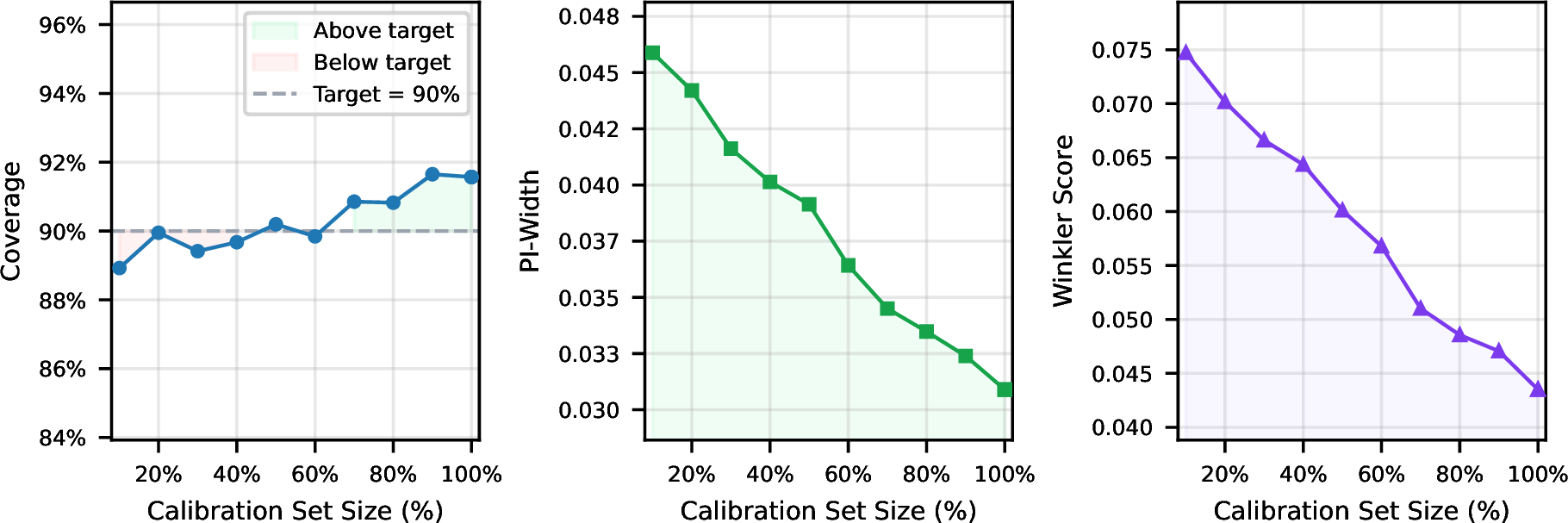
We examine how the size of the calibration set affects STOIC’s performance on the SCS dataset. We subsample this set to create calibration subsets ranging from 10% to the full size, while keeping the test set unchanged. For each subset, TabPFN is recalibrated and the resulting prediction intervals are evaluated using coverage, PI‑Width, and the Winkler score at the 90% target level. Figure 4 shows the three metrics as functions of the calibration fraction. Even when only 10% of the available calibration data is used, STOIC achieves a coverage of 88.92%, remaining remarkably close to the nominal 90% target. This result highlights the strength of the proposed calibration framework and demonstrates that reliable uncertainty estimates can be obtained from very limited calibration data. As the calibration set grows, coverage stabilizes around 90% and eventually slightly exceeds it, while the average interval width steadily decreases and the Winkler score improves. Importantly, the gains in sharpness are achieved without compromising calibration, indicating that additional calibration samples are primarily used to reduce uncertainty rather than to correct systematic coverage errors. This trend confirms that additional calibration samples allow the foundation model to estimate conditional quantiles more precisely, yielding sharper intervals without sacrificing coverage.
The observed behavior is particularly attractive from a practical deployment perspective. Many real-world forecasting systems initially operate with only a small amount of calibration data, especially when new assets, regions, or forecasting tasks are introduced. The results demonstrate that STOIC remains reliable even in such low-data regimes and improves gracefully as more calibration data become available. Second, increasing the calibration set size provides a predictable improvement in sharpness, making STOIC well‑suited for applications where historical data accumulates over time. Overall, these results demonstrate that STOIC combines strong calibration efficiency with robust uncertainty quantification, maintaining near-nominal coverage even under severe calibration data constraints while consistently benefiting from additional data. This ability to deliver reliable prediction intervals across both low- and high-data regimes makes STOIC particularly well-suited for real-world deployment scenarios.
6 Conclusion↩︎
In this paper, we proposed Spatial-Temporal Graph Conformal Prediction with In-Context Learning (STOIC), a novel framework for uncertainty quantification in energy demand forecasting. By decoupling point forecasting from interval estimation, STOIC addresses the inherent limitations of traditional conformal prediction when applied to spatially and temporally correlated network data. Our approach leverages the strengths of spatial-temporal graph neural networks to capture complex system dependencies while utilizing the zero-shot capabilities of tabular foundation models to perform adaptive and in-context calibration of residuals. Experimental results across five diverse benchmarks spanning synthetic simulations and real-world electricity and district heating datasets demonstrate that STOIC consistently delivers more reliable and data-efficient prediction intervals than existing baselines. Across all datasets, STOIC either matches or exceeds the target coverage level while maintaining competitive or substantially narrower prediction intervals, resulting in consistently strong Winkler scores. Specifically, the integration of in-context learning allows the framework to achieve well-calibrated coverage. The ablation studies further demonstrate that both spatial and temporal features contribute meaningfully to performance, while the TabPFN-based calibration module provides the largest individual gain, highlighting the importance of foundation-model-based calibration. Moreover, STOIC remains effective even when only a small calibration dataset is available, demonstrating strong data efficiency and making the framework particularly attractive for practical deployment scenarios where labeled calibration data are limited. This makes STOIC particularly suitable for modern sustainable energy systems characterized by high variability and evolving consumption patterns.
The comparison with TimesFM further highlights the importance of explicit calibration and domain-aware modeling. Despite being a large-scale pretrained forecasting model, TimesFM consistently fails to achieve the desired coverage levels on real-world energy datasets, whereas STOIC maintains reliable coverage while preserving competitive interval widths. This result demonstrates that large-scale pretraining alone is insufficient for reliable uncertainty quantification and that principled calibration remains essential for obtaining trustworthy prediction intervals in complex energy systems.
Overall, the results establish STOIC as an effective framework for uncertainty quantification in spatial-temporal forecasting problems, demonstrating that the combination of graph-based representations, conformal prediction, and foundation-model-based in-context learning provides a powerful and scalable approach for generating calibrated prediction intervals under spatial dependencies, temporal non-stationarity, and limited calibration data.
Future work can explore integrating a broader range of exogenous variables into the in-context prompt, such as real-time weather alerts, to further improve interval sharpness. Additionally, the STOIC framework can be extended to multi-horizon forecasting to enable robust uncertainty estimates for long-term strategic energy planning and grid stability assessments.
References↩︎
Part of this work was carried out during Keivan Faghih Niresi’s research visit at the Data, Vibration, and Uncertainty (DVU) Group, Department of Engineering, University of Cambridge.↩︎
https://archive.ics.uci.edu/dataset/321/electricityloaddiagrams20112014↩︎
https://axsa4prod4publicdata4sa.blob.core.windows.net/$web/index.html#dataset-a↩︎