A Geometry-Adaptive Regularized Newton-Type Method for Manifold-Affine Intersection Problems
June 30, 2026
Abstract
We propose a regularized algorithm, Regularized Newton-SLRA (RN-SLRA), for local manifold–affine intersection problems under weak intersection conditions, motivated in particular by structured low-rank approximation (SLRA). Newton-SLRA is an efficient method for manifold–affine intersection problems, but its well-definedness relies on the transversality condition between the manifold and the affine subspace, a condition that may fail in practice. RN-SLRA overcomes this difficulty by introducing a regularization term. We prove that, under the intrinsic transversality condition, RN-SLRA converges linearly to the intersection, while under the transversality condition it achieves higher-order convergence, including quadratic convergence for a suitable choice of the regularization parameter. We also study an inexact-projection variant, in which the projection onto the manifold is computed approximately, and show that the same local linear and quadratic convergence properties are preserved under the corresponding assumptions. Numerical experiments on constructed degenerate instances and Hankel-structured examples illustrate improved robustness in settings where Newton-SLRA may fail.
Manifold–affine intersection problems, structured low-rank approximation, regularization, inexact projection, intrinsic transversality, transversality, local convergence
65Y20, 65F55, 90C30
1 Introduction↩︎
Structured low-rank approximation (SLRA) seeks to approximate a given structured matrix (\(M\)) by a matrix (\(M_r\)) with the same structure and prescribed rank. We use SLRA mainly as a motivating setting for local manifold–affine intersection problems. Typical structures include Hankel, Toeplitz, Sylvester, and more general affine matrix structures [1], [2]. Unlike classical low-rank approximation, which is solved explicitly by the SVD, SLRA must enforce affine structure and rank constraints simultaneously. It arises in signal processing, system identification, and computer algebra [1], [3], [4]; low-rank Hankel approximation is related to exponential data fitting, frequency estimation, and denoising, while Sylvester-structured low-rank approximation is important in approximate polynomial GCD computations [1], [4], [5]. Geometrically, SLRA is a representative manifold–affine intersection problem, with the structure encoded by an affine subspace and the rank constraint by a smooth fixed-rank manifold.
Let \(\mathcal{M}_{p,q}(\mathbb{R})\) denote the space of real \(p\times q\) matrices, equipped with the Frobenius inner product \(\langle M_1,M_2\rangle=\operatorname{tr}(M_1^\top M_2)\) and norm \(\|M\|=\sqrt{\operatorname{tr}(M^\top M)}\). Denote by \(\mathcal{D}_r\) the subset of \(\mathcal{M}_{p,q}(\mathbb{R})\) consisting of matrices of rank \(r\). In the SLRA setting, all local statements involving \(\mathcal{D}_r\) are understood in a neighborhood of a rank-\(r\) point \(x^*\in E\cap\mathcal{D}_r\) with \(\sigma_r(x^*)>0\), where \(\mathcal{D}_r\) is a smooth fixed-rank manifold and the metric projection onto \(\mathcal{D}_r\) is locally single-valued. The local SLRA problem considered in this paper can be formulated as follows.
Consider an affine subspace \(E\subset \mathcal{M}_{p,q}(\mathbb{R})\), a matrix \(M\in E\), and an integer \(r\in \{0,1,\ldots,\min(p,q)\}\). Find a \(M_r\in E\cap\mathcal{D}_r\) close to \(M\).
Computing a metric projection onto \(E\cap \mathcal{D}_r\) is generally difficult. In practice, one usually seeks a nearby feasible point in \(E\cap \mathcal{D}_r\), which can be regarded as a local approximation to the projection onto the manifold–affine intersection. Many algorithms have been proposed for this purpose. Among them, the Cadzow algorithm [6], which alternates between the affine structure set and the fixed-rank manifold, is simple and robust, and converges locally linearly under separability-type intersection conditions [7], [8]. To obtain faster local convergence, Newton-SLRA [9] replaces the fixed-rank manifold by its tangent space at each iteration and achieves quadratic convergence under transversality. Other approaches include structured total least squares methods [10], [11], Riemannian optimization [12], [13], alternating minimization [14], variable projection [15], gradient systems [16], and algebraic methods [17].
The quadratic convergence of Newton-SLRA, however, relies on a restrictive geometric requirement: in the SLRA setting, the affine subspace \(E\) and the fixed-rank manifold \(\mathcal{D}_r\) must intersect transversally. When transversality fails, the tangent-space intersection in the Newton-SLRA update may be empty, and the associated linear system may become singular or severely ill-conditioned. Thus, although alternating projections remain applicable under weaker intersection conditions, the fast local behavior of Newton-SLRA is no longer available. This motivates the construction of a Newton-type method that is well defined under weaker geometry and recovers fast convergence under transversality.
To this end, we propose Regularized Newton-SLRA (RN-SLRA) for local manifold–affine intersection problems, with SLRA as a representative application. RN-SLRA replaces the exact tangent-space intersection step in Newton-SLRA by a regularized subproblem. Under intrinsic transversality, we prove local linear convergence of RN-SLRA and also record a local equivalence between intrinsic transversality and the two directional versions of separability in the \(C^2\) manifold–affine setting. Under transversality, we obtain faster local convergence by choosing \[\mu_k=c\,r_k^\rho,\qquad r_k:=d_{M}(x_k)=\|x_k-P_{M}(x_k)\|,\qquad c>0,\quad \rho\in[0,1].\] Since \(r_k\to0\), the regularization increasingly enforces the tangent-space condition underlying Newton-SLRA. With this choice, RN-SLRA converges locally with order at least \(1+\rho\), and in particular quadratically when \(\rho=1\). We call the method geometry-adaptive because the regularization parameter is chosen according to the manifold residual \(d_M(x_k)\), so that the step interpolates between alternating-projection behavior away from the intersection and Newton-SLRA behavior near the intersection.
For large-scale SLRA problems, the projection onto the fixed-rank manifold may itself be computationally expensive. We therefore further introduce Inexact Regularized Newton-SLRA (iRN-SLRA), which replaces the exact manifold projection by a \(\sigma\)-quasioptimal projection [18]. The inexact variant preserves the local convergence rates of RN-SLRA under the corresponding intersection assumptions, while allowing cheaper projection computations. The local convergence properties of the methods discussed above are summarized in Table 1.
| Intrinsic transversality | Transversality | |
|---|---|---|
| Cadzow (AP) | linear | linear |
| Newton-SLRA | – | quadratic |
| RN-SLRA (ours) | linear | order \(1+\rho\); quadratic if \(\rho=1\) |
| iRN-SLRA (ours) | linear | order \(1+\rho\); quadratic if \(\rho=1\) |
We evaluate RN-SLRA and iRN-SLRA on constructed degenerate SLRA instances and low-rank Hankel approximation problems at both small and large scales. The numerical results are consistent with the theoretical motivation above: on instances where transversality fails, RN-SLRA remains convergent, whereas Newton-SLRA may diverge. In addition, iRN-SLRA exhibits convergence behavior comparable to that of RN-SLRA while reducing the computational cost of the manifold projection step, with more pronounced savings on large-scale problems.
2 Preliminaries↩︎
We consider the general problem of approximating the projection of a point \(x\) onto the intersection \(X:=M\cap E\) of a smooth embedded manifold \(M\) and an affine subspace \(E\) in a Euclidean space, assuming without loss of generality that \(M\neq E\); in particular, the SLRA problem is recovered when \(M=\mathcal{D}_r\).
2.1 Notations and Basic Facts↩︎
We use \(d_C(x)\) to denote the distance from \(x\) to the set \(C\), and \(P_C(x)\) to represent the projection of \(x\) onto the set \(C\). \(B(x,r)\) denotes the ball centered at \(x\) with radius \(r\). We use \(\hat{u} = \frac{u}{\|u\|}\) to represent the unit vector of \(u\). For any affine subspace \(A\), let \(A^0\) denote its underlying vector space, so that \(A=x+A^0 \text{ for any }x\in A.\) In particular, we write \(E=x+L \text{ for any }x\in E,\) where \(L:=E^0\). For an affine manifold \(V\) and a point \(x\in V\), we denote by \(T_xV\) the affine tangent space of \(V\) at \(x\), and by \(N_xV\) the affine normal space of \(V\) at \(x\). Their underlying vector spaces are denoted by \(T_xV^0\) and \(N_xV^0\). \(L^{\perp}\) denotes the orthogonal complement of \(L\).
Assumption 1. \(E\) is an affine subspace and \(M\) is a smooth manifold of class \(C^2\).
We first recall some intersection conditions, including the transversality condition [7], [19], [20], the clean intersection condition [21], the intrinsic transversality condition [22], [23], the separability condition [24], and the subtransversality condition [25].
Definition 1 (Transversality). Let \(\mathbb{E}\) be a Euclidean space. Let \(M\subset \mathbb{E}\) be a manifold of class \(C^1\) and let \(E\) be an affine subspace of \(\mathbb{E}\). We say that \(E\) intersects \(M\) transversally at a point \(\bar x\in X\) if \[\operatorname{codim}(L \cap T_{\bar x} M^0) = \operatorname{codim}(L) + \operatorname{codim}(T_{\bar x} M^0).\]
We have the following lemma under transversality:
Lemma 1 (Uniform angle bound under transversality). Assume that \(E\) and \(M\) intersect transversally at \(\bar x\). Then, after possibly shrinking the neighborhood of \(\bar x\), there exists a constant \(\eta>0\) such that, for every \(y\in M\) sufficiently close to \(\bar x\) and every \(n\in N_yM^0\), \[\begin{align} \|P_L n\|\ge \eta \|n\|. \label{eq:53} \end{align}\qquad{(1)}\]
This lemma follows from [9]. A proof can be found in [26].
Definition 2 (Clean intersection). Let \(\mathbb{E}\) be a Euclidean space. Let \(M \subset \mathbb{E}\) be a manifold of class \(C^p(p\geq 2)\) and let \(E\) be an affine subspace of \(\mathbb{E}\). We say that \(E\) intersects \(M\) cleanly at a point \(\bar x\in X\) if the set \(X\) is a \(C^p\) embedded submanifold and \[T_x X = T_xM \cap L\] for all \(x\in X\) sufficiently close to \(\bar x\).
Definition 3 (Intrinsic Transversality). Let \(\mathbb{E}\) be a Euclidean space. Let \(M\subset\mathbb{E}\) be a manifold of class \(C^1\) and let \(E\) be an affine subspace of \(\mathbb{E}\). We say that \(E\) intersects \(M\) intrinsically transversally at a point \(\bar x\in X\) if there exists a constant \(\kappa>0\) such that for all \(x\in E\setminus M\) and \(y\in M\setminus E\) sufficiently close to \(\bar x\), \[\max \left\{ d\left( \widehat{x - y}, N_y M^0 \right), \; d\left( \widehat{x - y}, N_x E^0 \right) \right\} \ge \kappa.\]
Definition 4 (Separability). Let \(\mathbb{E}\) be a Euclidean space. Let \(M\subset\mathbb{E}\) be a manifold of class \(C^1\) and let \(E\) be an affine subspace of \(\mathbb{E}\). We say that \(E\) intersects \(M\) separably at a point \(\bar{x} \in X\) if there exists an angle \(\alpha > 0\) such that for any point \(z \in E \setminus M\) sufficiently close to \(\bar{x}\), and any points \(x \in P_M(z) \setminus E\) and \(z' \in P_E(x)\), the angle between the vectors \(z - x\) and \(z' - x\) is at least \(\alpha\).
The notion of separability was first introduced in [24] under the term 0-separability. This property is particularly suitable for the analysis of alternating projections and inexact alternating projection methods [8].
In our work, intrinsic transversality serves as the main geometric assumption for the local linear convergence analysis.
Assumption 2. \(E\) intersects \(M\) intrinsically transversally at \(\bar x\).
Under Assumption 1, intrinsic transversality is equivalent to separability in either order; see Lemma 2 below. Although separability is not symmetric in general, in the present \(C^2\) manifold–affine setting the two directional versions are equivalent. More precisely, \(E\) intersects \(M\) separably at \(\bar x\) if and only if \(M\) intersects \(E\) separably at \(\bar x\), and these are both equivalent to intrinsic transversality.
Lemma 2. Let \(\mathbb{E}\) be a Euclidean space, let \(M \subset \mathbb{E}\) be a \(C^2\) manifold, and let \(E \subset \mathbb{E}\) be an affine subspace. Then the following are equivalent at \(\bar x \in E \cap M\):
\(E\) intersects \(M\) separably at \(\bar x\);
\(M\) intersects \(E\) separably at \(\bar x\);
\(E\) intersects \(M\) intrinsically transversally at \(\bar x\).
Proof. Write \(E=\bar x+L\), so \(N_x E=L^\perp\) for all \(x\in E\).
\((1)\Rightarrow(2)\). Assume that \(E\) intersects \(M\) separably at \(\bar x\). After possibly shrinking \(U\), we may assume that \(P_E(M\cap U)\subset U\) and \(P_M(E\cap U)\subset U\) by continuity of \(P_E\) at \(\bar x\) and local single-valuedness and continuity of \(P_M\) near \(\bar x\).
Take \(y\in (M\cap U)\setminus E,\;x=P_E(y)\in U\setminus M,\;y^+\in P_M(x)\cap U,\) and set \(x^+:=P_E(y^+)\). If \(y^+\in E\), then \(y^+-x\in L,\;y-x\in L^\perp,\) hence \(\angle(y-x,y^+-x)=\frac{\pi}{2}\ge \alpha.\) Assume now \(y^+\notin E\). Since \(x\in E\), \(y^+\in P_M(x)\setminus E\), and \(x^+=P_E(y^+)\), separability gives \(\angle(x-y^+,x^+-y^+)\ge \alpha.\) Moreover, \(x^+-y^+ = P_{L^\perp}(x-y^+)\) and \(x-y\in L^\perp\). By Cauchy’s inequality, among all nonzero vectors \(w\in L^\perp\), the angle between \(x-y^+\) and \(w\) is minimized when \(w\) is parallel to \(P_{L^\perp}(x-y^+)\). Hence \(\angle(x-y^+,x-y) \ge \angle(x-y^+,x^+-y^+) \ge \alpha .\) Equivalently, \(\angle(y-x,y^+-x)\ge \alpha.\) Thus \(M\) intersects \(E\) separably at \(\bar x\).
\((2)\Rightarrow(3)\). Assume that \(M\) intersects \(E\) separably at \(\bar x\), but intrinsic transversality fails. Then there exist \(a_k\in E\setminus M,\;y_k\in M\setminus E,\;a_k\to\bar x,\;y_k\to\bar x,\) such that, with \(w_k:=\widehat{y_k-a_k}\), \[\max\{d(w_k,L^\perp),\,d(w_k,N_{y_k}M^0)\}\to 0.\] Set \(x_k:=P_E(y_k),\;t_k:=\|y_k-x_k\|,\;u_k:=\frac{y_k-x_k}{\|y_k-x_k\|}.\) Then \(u_k\in L^\perp\) and \(P_{L^\perp}(y_k-a_k)=y_k-x_k, \; P_{L^\perp}w_k=\frac{t_k}{\|y_k-a_k\|}u_k.\) Since \(d(w_k,L^\perp)\to0\), we have \(\|P_{L^\perp}w_k\|\to1\), hence \(u_k=\frac{P_{L^\perp}w_k}{\|P_{L^\perp}w_k\|}\to w_k.\) Choose \(v_k\in N_{y_k}M^0\) with \(\|v_k-w_k\|=d(w_k,N_{y_k}M^0)\to0\). Then \(\|u_k-v_k\|\to 0.\) Define \(z_k:=y_k-t_kv_k.\) Since \(M\) is a \(C^2\) manifold, for all large \(k\), \(z_k\) lies in a tubular neighborhood of \(M\) and \(P_M(z_k)=y_k.\) Moreover, \(P_M\) is locally Lipschitz there. As \(x_k=y_k-t_ku_k, \; z_k-x_k=t_k(u_k-v_k),\) we obtain \[\|z_k-x_k\|=t_k\|u_k-v_k\|=o(t_k), \qquad \|z_k-y_k\|=t_k.\] Hence, for all large \(k\), necessarily \(x_k\notin M\); otherwise \(x_k\) would be closer to \(z_k\) than \(y_k\), contradicting \(P_M(z_k)=y_k\).
Now let \(y_k^+:=P_M(x_k)\). By local Lipschitz continuity of \(P_M\), \[\|y_k^+-y_k\| = \|P_M(x_k)-P_M(z_k)\| \le C\|x_k-z_k\| =o(t_k).\] Since \(\|y_k-x_k\|=t_k\), it follows that \(\|(y_k^+-x_k)-(y_k-x_k)\|=o(t_k),\) and therefore \(\angle(y_k-x_k,y_k^+-x_k)\to0.\) But for all large \(k\), \(y_k\in M\setminus E,\;x_k=P_E(y_k)\in E\setminus M,\;y_k^+\in P_M(x_k),\) so separability of \(M\) relative to \(E\) yields some \(\alpha_0>0\) such that \(\angle(y_k-x_k,y_k^+-x_k)\ge \alpha_0,\) a contradiction. Hence \(E\) and \(M\) are intrinsically transversal at \(\bar x\).
\((3)\Rightarrow(1)\). This follows from the fact that intrinsic transversality implies separability; see [24].
Therefore \((1)\), \((2)\), and \((3)\) are equivalent. ◻
Definition 5 (Subtransversality). Let \(\mathbb{E}\) be a Euclidean space. Let \(M\subset\mathbb{E}\) be a manifold of class \(C^1\) and let \(E\) be an affine subspace of \(\mathbb{E}\). We say that \(E\) intersects \(M\) subtransversally at a point \(\bar{x} \in X\) if there exist constants \(\tau > 0\) and a neighborhood \(U\) of \(\bar{x}\) such that for all \(w \in U\), \[d(w, X) \le \tau \left( d(w, E) + d(w, M) \right).\]
Under the present \(C^2\) embedded manifold–affine setting and with the definitions used here, the following relationships hold locally, rather than as unconditional statements for arbitrary sets: transversality implies clean intersection; clean intersection is equivalent to intrinsic transversality[27]; intrinsic transversality implies subtransversality; and intrinsic transversality is equivalent to separability in either order. See [23], [24], [27].
2.2 Cadzow Algorithm↩︎
The alternating projection (AP) method has a long history [28], [29]. Recent studies have analyzed AP and inexact AP methods for various sets [30]–[32], together with their local linear convergence properties [8], [24], [31], [33]. In the context of structured low-rank approximation, the Cadzow algorithm [6], [34] can be viewed as an alternating projection method between the affine space \(E\) and the low-rank manifold \(M\). More precisely, starting from \(x_k\in E\), one step of the Cadzow iteration is given by \[\begin{align} x_{k+1}=P_E P_M(x_k). \end{align}\]
In the local rank-\(r\) neighborhood considered in this paper, the projection onto \(\mathcal{D}_r\) is computed by the truncated SVD, as a local consequence of the Eckart–Young theorem:
Lemma 3 (Eckart-Young Theorem). Let \(x\in\mathcal{M}_{p,q}(\mathbb{R})\) be a matrix, and let \(r\) be a positive integer not greater than \(\min(p,q)\). Let \(x=USV^\top\) be its SVD, where \(S=\mathop{\mathrm{diag}}(\sigma_1,\cdots,\sigma_{\min(p,q)})\) with \(\sigma_1\geq \cdots \geq \sigma_{\min(p,q)}\geq 0\). If \(x\) is sufficiently close to a rank-\(r\) point \(x^*\) with \(\sigma_r(x^*)>0\), then a projection \(P_{\mathcal{D}_r}(x)\) is given by \[P_{\mathcal{D}_r}(x)=U\tilde{S}V^\top,\;\;\tilde{S}=\mathop{\mathrm{diag}}(\sigma_1,\cdots,\sigma_r,0,\cdots,0).\]
Then Cadzow algorithm can be formulated as: \[\begin{align} &U,S,V \leftarrow \text{SVD}(x_k),\qquad y_k=U_rS_rV_r^\top, \\ &x_{k+1}=x_k+\sum_{i=1}^d \langle y_k-x_k,E_i \rangle E_i. \end{align}\] where \(U_r\) denotes the matrix consisting of the first \(r\) columns of \(U\), \(V_r\) denotes the matrix consisting of the first \(r\) columns of \(V\), \(S_r\) denotes the \(r\times r\) top-left submatrix of \(S\), \(d\) is the dimension of \(E\), and \(\{E_i\}_{i=1}^d\) denotes an orthonormal basis of \(L\). The update formula for \(x_{k+1}\) is obtained by \[x_{k+1}=P_E(y_k)=x_k+P_L(y_k-x_k).\]
If \(E\) intersects \(M\) transversally at \(\bar x\in X\) and the initial point is sufficiently close to \(\bar x\), the Cadzow algorithm will converge locally linearly to a point \(x_{\infty}\in X\) [7]. In fact, local linear convergence can already be guaranteed when \(E\) intersects \(M\) separably [8].
2.3 Newton-SLRA Algorithm↩︎
The Newton-SLRA algorithm is motivated by Newton’s method. In each iteration of the classical Newton-SLRA, given the current iterate \(x_k \in E\), one first computes its projection onto the manifold \(y_k = P_{M}(x_k)\), and then solves a linear least-squares problem: \(x_{k+1} = P_{E \cap T_{y_k}M}(x_k),\) i.e., the closest point to \(x_k\) in the intersection of \(E\) and the tangent space \(T_{y_k}M\). Under the transversality condition, this algorithm converges locally quadratically. When \(M=\mathcal{D}_r\), the algorithm can be formulated as: \[\label{eq:newton-slra} \begin{align} &U,S,V\leftarrow \mathrm{SVD}(x_k),\qquad y_k = U_r S_r V_r^\top,\\ &N_{ij}\leftarrow u_i v_j^\top,\quad i=r+1,\dots,p,\;\;j=r+1,\dots,q,\\ &A\leftarrow \big(\langle N_{ij},E_\ell\rangle\big)_{(i,j),\ell}, \qquad b\leftarrow \big(\langle N_{ij},\,y_k-x_k\rangle\big)_{(i,j)},\\ &x_{k+1}=x_k+\displaystyle\sum_{\ell=1}^d (A^\dagger b)_\ell E_\ell. \end{align}\tag{1}\]
However, when transversality fails, the matrix \(A\) in 1 may lose rank at the solution. In the fixed-rank SLRA setting, full row rank of the tangent-space linear system is equivalent to transversality of \(E\) and \(\mathcal{D}_r\) at the intersection point. Hence, near a nontransversal solution, the associated least-squares problem may become singular or severely ill-conditioned.
Another issue is that the well-definedness of Newton-SLRA relies on the non-emptiness of \(E \cap T_{y_k} M\). Under transversality, there exists a positive lower bound \(\alpha\) for the angle between \(E\) and \(T_{y_k} M\) in some neighborhood of \(\bar{x}\), but this cannot be guaranteed under intrinsic transversality, as \(E \cap T_{y_k} M\) may be empty.
These issues inspired us to modify the Newton-SLRA algorithm to design a new algorithm, called Regularized Newton-SLRA (RN-SLRA), which is able to handle the above issues.
3 Regularized Newton-SLRA↩︎
We introduce a regularization term and define the next iterate as: \[\label{eq:rnslra} \begin{align} &y_k=P_M(x_k),\\ &x_{k+1} = \arg\min_{x \in E} \left\{ \dfrac{1}{2} \| x - y_k \|^2 + \dfrac{1}{2\mu_k} \| P_{N_{y_k}M}(x - y_k) \|^2 \right\}, \quad \mu_k > 0. \end{align}\tag{2}\] where \(P_{N_{y_k}M}\) is the orthogonal projector onto the normal space \(N_{y_k}M\), and \(\mu_k\) is a regularization parameter. In the algorithm studied below, \(\mu_k\) is chosen adaptively according to: \[\mu_k = c \cdot r(x_k)^\rho,\quad r(x_k)=\|x_k-y_k\|=d_M(x_k).\] where \(c>0\) is a constant, \(0\le\rho\le 1\) is a parameter. This choice of the regularization parameter is inspired by the residual-dependent regularization strategy used in the Inexact Regularized Proximal Newton method (IRPN) [35], and is also related to earlier regularized Newton methods for convex minimization with singular solutions [36] as well as improved proximal Newton implementations such as newGLMNET [37].
Since \(E\) is affine, the objective function in 2 for solving \(x_{k+1}\) is a strongly convex quadratic problem with a unique solution, which can be obtained by solving a linear system. Thus, the well-definedness of the RN-SLRA step does not require the transversality condition between \(E\) and \(M\).
3.1 Derivation of the Linear System↩︎
Let \(\{E_1,\dots,E_d\}\) be an orthonormal basis of \(L\), set \(b=x_k-y_k\), and write \(N=N_{y_k}M\). Choose an orthonormal basis \(\{N_j\}_{j=1}^s\) of \(N\). Since \(E=x_k+L\), any \(x\in E\) can be written as \(x=y_k+b+\sum_{i=1}^d\alpha_iE_i\). Substituting this expression into 2 and using the first-order optimality condition gives \[\begin{align} \label{eq:sys} \left(I_d+\frac{1}{\mu_k}A^\top A\right)\alpha = -\beta-\frac{1}{\mu_k}A^\top \eta, \end{align}\tag{3}\] where \(A_{ji}=\langle N_j,E_i\rangle, \eta_j=\langle N_j,b\rangle,\) and \(\beta_i=\langle b,E_i\rangle.\) Since \(A^\top A\succeq0\) and \(\mu_k>0\), the coefficient matrix is positive definite. The next iterate is \(x_{k+1}=x_k+\sum_{i=1}^d\alpha_iE_i\).
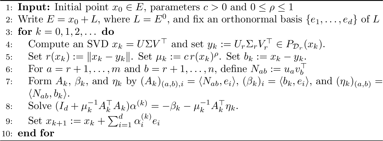
For the fixed-rank manifold \(M=\mathcal{D}_r\), this yields Algorithm 1.
3.2 Limiting Interpretation of the Regularized Step↩︎
Assume that \(E\) and \(M\) intersect transversally at \(\bar x\), so that \(E\cap T_{y_k}M\) is nonempty for \(y_k\) sufficiently close to \(\bar x\). The role of \(\mu_k\) can be understood from two limiting regimes.
If \(\mu_k\to\infty\), the penalty term vanishes and the subproblem reduces to \(\min_{x\in E}\|x-y_k\|^2\). Hence the step becomes \(p_k=P_E(y_k)\), namely the alternating projection step. If \(\mu_k \to 0\), the penalty term enforces \(P_{N_{y_k}M}(x-y_k)=0\), or equivalently \(x\in T_{y_k}M\). Thus the limiting problem is \(\min_{x\in E\cap T_{y_k}M} \|x-y_k\|^2 .\) Since \(y_k=P_M(x_k)\), we have \(x_k-y_k\in N^0_{y_k}M\). Hence, for every \(x\in T_{y_k}M\), \(\|x-x_k\|^2 = \|x-y_k\|^2+\|x_k-y_k\|^2 .\) Therefore, minimizing the distance to \(y_k\) over \(E\cap T_{y_k}M\) is equivalent to minimizing the distance to \(x_k\) over the same set. The limiting step is the Newton–SLRA point \(q_k=P_{E\cap T_{y_k}M}(x_k),\) provided that \(E\cap T_{y_k}M\) is nonempty.
Thus, for \(\mu_k\in(0,\infty)\), the regularized step interpolates between alternating projections and Newton-SLRA: smaller \(\mu_k\) gives a more Newton-like step, while larger \(\mu_k\) gives a more projection-like step. This interpretation relies on the local nonemptiness of \(E\cap T_{y_k}M\), which follows from transversality but may fail under Assumption 2; it is used only as intuition and not in the convergence analysis below.
3.3 Inexact Regularized Newton-SLRA↩︎
We replace \(y_k=P_M(x_k)\) in 2 by a quasioptimal projection and obtain iRN-SLRA: \[\label{eq:iRN-SLRA} \begin{align} &y_k\in M \;\text{such that}\;\|x_k-y_k\|\le \sigma\, d_M(x_k), \quad \sigma\ge 1, \\ &x_{k+1}=\displaystyle \arg\min_{x\in E} \left\{ \frac{1}{2}\|x-y_k\|^2 +\frac{1}{2\mu_k}\bigl\|P_{N_{y_k}M}(x-y_k)\bigr\|^2 \right\}, \quad \mu_k>0. \end{align}\tag{4}\] When \(\sigma=1\), iRN-SLRA reduces to RN-SLRA. For \(\sigma>1\), \(y_k\) is a \(\sigma\)-quasioptimal projection of \(x_k\) onto \(M\), in the sense of [18]. This quasioptimal model is well suited to low-rank approximation: truncated SVD gives the exact projection with \(\sigma=1\), while randomized SVD provides a practical realization in expectation or with high probability under standard randomized low-rank approximation bounds [38]; partial SVD can also be used in practice [39]. Compared with a full SVD, these approaches can significantly reduce the computational cost, especially for large-scale problems.
For an \(m\times n\) rank-\(r\) SLRA problem with affine dimension \(d\), one RN-SLRA iteration consists of: (i) computing the rank-\(r\) projection, implemented by a truncated or full SVD; (ii) forming the normal-coordinate matrix \(A_k\in\mathbb{R}^{(m-r)(n-r)\times d}\); and (iii) solving a \(d\times d\) symmetric positive definite linear system. Thus the dominant cost is typically the rank-\(r\) projection and the construction of \(A_k\), while the \(d\times d\) solve is moderate when \(d\) is small or structured. For Hankel/Toeplitz structures, the affine basis and matrix-vector products can often be represented implicitly, and randomized or partial SVD can reduce the projection cost in large-scale settings.
4 Local Convergence Analysis↩︎
In this section, we establish the local convergence properties of the proposed algorithms. We first prove that RN-SLRA converges linearly under intrinsic transversality. We then show that, under the stronger transversality condition, the convergence rate improves to quadratic convergence. Finally, we extend the analysis to the inexact variant iRN-SLRA. Throughout this section, \(\{x_k\}\) denotes the sequence of iterates generated by the corresponding algorithm.
4.1 Linear Convergence of RN-SLRA under Intrinsic Transversality↩︎
Lemma 4. Suppose that Assumptions 1 and 2 hold. There exist constants \(\delta_1>0\) and \(\kappa>0\) such that, for every \(y\in M\cap B(\bar x,\delta_1)\), \[d_{X}(y)\leq \kappa\, d_E(y).\]
Lemma 5. Suppose that Assumptions 1 and 2 hold. There exist constants \(\delta_2>0\) and \(\kappa'>0\) such that, for every \(x\in E\cap B(\bar x,\delta_2)\), \[d_{X}(x)\leq \kappa' d_M(x).\]
Both of the above lemmas can be derived from subtransversality, which itself follows from intrinsic transversality. These two lemmas show that there exists a neighborhood \(U\) of \(\bar x\) such that the distance from a point in \(E\cap U\) to \(M\), or from a point in \(M\cap U\) to \(E\), is of the same order as its distance to \(X\).
Suppose that Assumption 1 holds. Then, after possibly shrinking the neighborhood of \(\bar x\), there exist constants \(\eta,G,G'>0\) such that the following hold for all points sufficiently close to \(\bar x\):
for all \(y,z\in M\), \[\|P_{N_yM^0}(z-y)\|\le \eta \|z-y\|^2; \label{eq:normal-quadratic-prop}\tag{5}\]
for all \(y\in M\) and all \(x\) sufficiently close to \(y\), \[d_M(x)\le \|P_{N_yM^0}(x-y)\|+G\|x-y\|^2; \label{eq:distance-normal-upper-prop}\tag{6}\]
for all \(y\in M\) and all \(x\) sufficiently close to \(y\), \[\|P_{N_yM^0}(x-y)\|\le d_M(x)+G'\|x-y\|^2. \label{eq:distance-normal-lower-prop}\tag{7}\]
Proof. By the local \(C^2\) geometry of \(M\), for each \(y\in M\) near \(\bar x\) and each \(u\in T_yM^0\) small, points of \(M\) near \(y\) can be represented as \(y+u+v_y(u)\) with \(v_y(u)\in N_yM^0\). Here \(v_y(0)=0\) and \(Dv_y(0)=0\); equivalently, after shrinking the neighborhood, \(\|v_y(u)\|\le c\|u\|^2\) uniformly for \(y\) near \(\bar x\); see [40]. Therefore, if \(z\in M\) is close to \(y\) and \(u=P_{T_yM^0}(z-y)\), then \(z-y=u+v_y(u),\) so \(P_{N_yM^0}(z-y)=v_y(u),\) which gives 5 .
Next, for \(x\) close to \(y\), let \(u=P_{T_yM^0}(x-y)\) and set \(w:=y+u+v_y(u)\in M\). Then \(x-w=P_{N_yM^0}(x-y)-v_y(u),\) and hence \[d_M(x)\le \|x-w\| \le \|P_{N_yM^0}(x-y)\|+c\|u\|^2 \le \|P_{N_yM^0}(x-y)\|+c\|x-y\|^2,\] which proves 6 .
Finally, let \(p:=P_M(x)\). Since the metric projection onto \(M\) is single-valued near \(M\) [7], applying 5 to \(y,p\in M\) yields \(\|P_{N_yM^0}(p-y)\|\le \eta\|p-y\|^2.\) Thus \[\|P_{N_yM^0}(x-y)\| \le \|P_{N_yM^0}(x-p)\|+\|P_{N_yM^0}(p-y)\| \le d_M(x)+\eta\|p-y\|^2.\] Since \(\|p-y\|\le \|p-x\|+\|x-y\|\le 2\|x-y\|\), 7 follows. ◻
Lemma 6 (Step-size estimate). Suppose that Assumptions 1 and 2 hold. There exist \(\delta_3>0\) and \(C_1>0\) such that, for all iterates \(x_k\in E\cap B(\bar x,\delta_3)\), \[\|x_{k+1}-x_k\|\le C_1\,r(x_k).\]
Proof. Let \(r_k:=r(x_k)=d_M(x_k),\;y_k:=P_M(x_k).\) Since \(x_k\in E\), we have \(d_E(y_k)\le \|y_k-x_k\|=r_k.\) Hence, by Lemma 4, after shrinking the neighborhood if necessary, there exists \(\kappa>0\) such that \(d_X(y_k)\le \kappa\, d_E(y_k)\le \kappa r_k .\) Choose \(z_k\in P_X(y_k)\). Then \[\begin{align} \|z_k-y_k\|=d_X(y_k)\le \kappa r_k . \label{eq:5} \end{align}\tag{8}\]
Now define the regularized objective \[\Phi_k(x):=\frac{1}{2}\|x-y_k\|^2+\frac{1}{2\mu_k}\|P_{N_{y_k}M}(x-y_k)\|^2, \qquad x\in E.\] By construction, \(x_{k+1}\) minimizes \(\Phi_k\) over \(E\), so \[\begin{align} \Phi_k(x_{k+1})\le \Phi_k(z_k). \label{eq:6} \end{align}\tag{9}\]
Next we estimate the normal component of \(z_k-y_k\). Since \(M\) is a \(C^2\) manifold near \(\bar x\) (by Assumption 1), applying 5 with \(y=y_k\) and \(z=z_k\) and using 8 , one has \[\begin{align} \|P_{N_{y_k}M}(z_k-y_k)\| \le \eta \|z_k-y_k\|^2 \le \eta \kappa^2 r_k^2 . \label{eq:8} \end{align}\tag{10}\]
Therefore, \[\begin{align} \Phi_k(z_k) = \frac{1}{2}\|z_k-y_k\|^2 +\frac{1}{2\mu_k}\|P_{N_{y_k}M}(z_k-y_k)\|^2 \le \frac{1}{2}\kappa^2 r_k^2 +\frac{1}{2\mu_k}\eta^2\kappa^4 r_k^4 . \label{eq:9} \end{align}\tag{11}\] Using \(\mu_k=c\,r_k^\rho\) with \(c>0\) and \(0\le \rho\le 1\), we get \[\begin{align} \Phi_k(z_k) \le \frac{1}{2}\kappa^2 r_k^2 +\frac{\eta^2\kappa^4}{2c} r_k^{4-\rho}. \label{eq:10} \end{align}\tag{12}\] Since \(4-\rho\ge 3>2\), after shrinking the neighborhood further we may assume \(r_k\le 1\), and hence \(\Phi_k(z_k)\le C\, r_k^2\) for some constant \(C>0\) independent of \(k\).
Since the second term in \(\Phi_k\) is nonnegative, this bound and 9 imply \(\frac{1}{2}\|x_{k+1}-y_k\|^2\le \Phi_k(x_{k+1})\le C r_k^2 ,\) and therefore \[\begin{align} \|x_{k+1}-y_k\|\le \sqrt{2C}\, r_k . \label{eq:14} \end{align}\tag{13}\] Finally, by the triangle inequality, \[\begin{align} \|x_{k+1}-x_k\| \le \|x_{k+1}-y_k\|+\|y_k-x_k\| \le \sqrt{2C}\, r_k+r_k = (1+\sqrt{2C})\, r_k . \end{align}\] Thus the conclusion holds with \(C_1:=1+\sqrt{2C}.\) This proves the lemma. ◻
Lemma 7 (Residual contraction). Suppose that Assumptions 1 and 2 hold. There exist \(\delta>0\), \(q\in(0,1)\), and \(C_2>0\) such that, for all \(x_k\in E\cap B(\bar x,\delta)\), \[r(x_{k+1}) \le q\,r(x_k)+C_2\,r(x_k)^2.\]
Proof. Write \(r_k:=r(x_k)=d_M(x_k),\;y_k:=P_M(x_k),\;N_k:=N_{y_k}M,\) and set \(p_k:=P_E(y_k).\) Since \(E=\bar x+L\) is affine, we have \(p_k-y_k\in L^\perp,\;x_{k+1}-p_k\in L.\)
By 6 , after shrinking the neighborhood of \(\bar x\) if necessary, there exists \(G>0\) such that \[\begin{align} r(x_{k+1}) \le \|P_{N_k}(x_{k+1}-y_k)\|+G\|x_{k+1}-y_k\|^2 . \label{eq:16} \end{align}\tag{14}\]
Now \(x_{k+1}\) minimizes \[x\mapsto \frac{1}{2}\|x-y_k\|^2+\frac{1}{2\mu_k}\|P_{N_k}(x-y_k)\|^2 \qquad\text{over }E=p_k+L,\] so the first-order optimality condition is obtained by requiring the gradient to be orthogonal to the feasible direction space \(L\), namely \[P_L\!\left[(x_{k+1}-y_k)+\frac{1}{\mu_k}P_{N_k}(x_{k+1}-y_k)\right]=0.\] Using \(P_L(p_k-y_k)=0\), this gives \(x_{k+1}-y_k = (p_k-y_k)-\frac{1}{\mu_k}P_LP_{N_k}(x_{k+1}-y_k).\) Applying \(P_{N_k}\) to this identity and rearranging terms, we obtain \[\begin{align} \left(I+\frac{1}{\mu_k}P_{N_k}P_L\right)P_{N_k}(x_{k+1}-y_k) = P_{N_k}(p_k-y_k). \label{eq:18} \end{align}\tag{15}\]
Consider the operator \[\begin{align} \label{eq:bk} B_k:=I+\frac{1}{\mu_k}P_{N_k}P_L:N_k\to N_k. \end{align}\tag{16}\] For any \(n\in N_k\), \(\langle B_kn,n\rangle = \|n\|^2+\frac{1}{\mu_k}\|P_Ln\|^2 \ge \|n\|^2.\) Hence \(B_k\) is invertible and \(\|B_k^{-1}\|\le 1\). Therefore, from 15 , \[\begin{align} \|P_{N_k}(x_{k+1}-y_k)\| \le \|P_{N_k}(p_k-y_k)\|. \label{eq:19} \end{align}\tag{17}\]
Next, by 7 , there exists \(G'>0\) such that \[\begin{align} \|P_{N_k}(p_k-y_k)\| \le d_M(p_k)+G'\|p_k-y_k\|^2. \label{eq:20} \end{align}\tag{18}\]
Since \(p_k=P_E(y_k)\) and \(x_k\in E\), \[\begin{align} \|p_k-y_k\|=d_E(y_k)\le \|x_k-y_k\|=r_k. \label{eq:21} \end{align}\tag{19}\] Moreover, \(p_k=P_E(P_M(x_k))\) is one alternating-projection step from \(x_k\in E\). By the one-step decrease estimate underlying [23], intrinsic transversality implies that, after shrinking the neighborhood if necessary, there exists \(q\in(0,1)\) such that \[\begin{align} d_{M}(p_k)\le q\,d_M(x_k) = q r_k . \label{eq:22} \end{align}\tag{20}\] Combining 18 20 , we obtain \[\begin{align} \|P_{N_k}(p_k-y_k)\| \le q\,r_k+G'r_k^2. \label{eq:23} \end{align}\tag{21}\] Hence, by 17 , \[\begin{align} \|P_{N_k}(x_{k+1}-y_k)\| \le q\,r_k+G'r_k^2. \label{eq:24} \end{align}\tag{22}\]
Substituting 22 into 14 and using 13 , we arrive at \(r(x_{k+1}) \le q\,r_k+G'r_k^2+2CGr_k^2 \le q\,r(x_k)+C_2r(x_k)^2\) for some \(C_2>0\). This completes the proof. ◻
In the above proof, we introduced the operator \(B_k=I+\frac{1}{\mu_k}P_{N_k}P_L: N_k\to N_k\) in 16 , and established the bound \(\|B_k^{-1}\|\le 1\). We emphasize that a sharper estimate requires a uniform lower bound on the action of \(P_L\) on \(N_k\). More precisely, under transversality one has, after shrinking the neighborhood if necessary, there exists \(\eta>0\) such that \(\|P_L n\|\ge \eta\|n\|\) for all \(n\in N_k\). Equivalently, \(P_{N_k}P_L|_{N_k}\) is uniformly positive definite on \(N_k\). We will use this stronger estimate in Theorem 3.
The following result is a direct corollary of the previous lemma.
Corollary 1. Suppose that Assumptions 1 and 2 hold. There exist constants \(\tau\in(0,1)\) and \(C_r>0\) such that, for any initial point \(x_0\in E\) sufficiently close to \(\bar x\), the sequence \(\{x_k\}\) generated by Algorithm RN-SLRA satisfies \[r(x_k)\le C_r \tau^k,\qquad k=0,1,2,\dots.\] In particular, \(\{r(x_k)\}\) converges \(Q\)-linearly to \(0\).
Proof. By Lemma 7, there exist \(q\in(0,1)\), \(C_2>0\) and \(\delta>0\) such that, for \(x_k\in E\cap B(\bar x,\delta)\), \[\begin{align} r(x_{k+1}) \le q\,r(x_k)+C_2\,r(x_k)^2 . \label{eq:29} \end{align}\tag{23}\] Choose \(\varepsilon>0\) with \(\tau:=q+C_2\varepsilon<1\), and shrink \(\delta\) so that \(r(x)\le\varepsilon\) on \(E\cap B(\bar x,\delta)\). By Lemma 6, after shrinking \(\delta\) further, we have \(\|x_{k+1}-x_k\|\le C_1r(x_k)\) whenever \(x_k\in E\cap B(\bar x,\delta)\). Take \(x_0\in E\) so close to \(\bar x\) that \(\|x_0-\bar x\|+\frac{C_1}{1-\tau}r(x_0)<\delta .\) We prove by induction that \(x_k\in B(\bar x,\delta)\) and \(r(x_k)\le \tau^k r(x_0)\). Indeed, if this holds up to \(k\), then \(r(x_k)\le\varepsilon\), so 23 gives \[r(x_{k+1})\le (q+C_2r(x_k))r(x_k)\le \tau r(x_k) \le \tau^{k+1}r(x_0),\] and \[\|x_{k+1}-\bar x\| \le \|x_0-\bar x\|+C_1\sum_{j=0}^{k}r(x_j) \le \|x_0-\bar x\|+\frac{C_1}{1-\tau}r(x_0)<\delta .\] Thus \(r(x_k)\le r(x_0)\tau^k\) for all \(k\). Thus \(r(x_k)\le r(x_0)\tau^k\le C_r\tau^k\), after possibly shrinking the initial neighborhood so that \(r(x_0)\le C_r\). ◻
Theorem 1. Suppose that Assumptions 1 and 2 hold. For every initial point \(x_0\in E\) sufficiently close to \(\bar x\), the sequence \(\{x_k\}\) generated by Algorithm RN-SLRA converges to some point \(x_\infty\in X\). Moreover, there exist constants \(C_X,C_s,C_\infty>0\) and \(\tau\in(0,1)\) such that \[\begin{align} \label{eq:33} d_X(x_k) \le C_X \tau^k, \quad \|x_{k+1}-x_k\| \le C_s \tau^k, \quad \|x_k-x_\infty\| \le C_\infty \tau^k \end{align}\qquad{(2)}\] for all \(k=0,1,2,\dots\).
Proof. By Corollary 1, there exist \(\tau\in(0,1)\) and \(C_r>0\) such that \(r(x_k)\le C_r\tau^k\) for all \(k=0,1,2,\dots\). On the other hand, by Lemma 5, after possibly shrinking the neighborhood of \(\bar x\), there exists \(\kappa'>0\) such that \(d_X(x)\le \kappa' r(x)\) for all \(x\in E\) in this neighborhood. Hence \(d_X(x_k)\le \kappa' C_r\tau^k\), and the first estimate in ?? holds with \(C_X:=\kappa' C_r\).
Next, by Lemma 6, there exists \(C_1>0\) such that \(\|x_{k+1}-x_k\|\le C_1 r(x_k)\). Therefore \(\|x_{k+1}-x_k\|\le C_1C_r\tau^k\), which proves the second estimate in ?? with \(C_s:=C_1C_r\).
Since \(\tau\in(0,1)\), it follows that \(\sum_{k=0}^\infty\|x_{k+1}-x_k\|<\infty\). Thus \(\{x_k\}\) is a Cauchy sequence in \(E\), and hence converges to some \(x_\infty\in E\). Moreover, \(d_X(x_\infty)\le d_X(x_k)+\|x_k-x_\infty\|\to0\), where the convergence follows from the first estimate in ?? . Hence \(x_\infty\in X\) because \(X\) is closed.
Finally, for every \(k\), \[\begin{align} \|x_k-x_\infty\| \le \sum_{j=k}^\infty \|x_{j+1}-x_j\| \le C_1 C_r \sum_{j=k}^\infty \tau^j = \frac{C_1 C_r}{1-\tau}\tau^k. \label{eq:42} \end{align}\tag{24}\] Thus the third estimate in ?? holds with \(C_\infty:=\dfrac{C_1 C_r}{1-\tau}\). ◻
Corollary 2. Suppose that Assumptions 1 and 2 hold. For every initial point \(x_0\in E\) sufficiently close to \(\bar x\), the sequences \(\{d_X(x_k)\}\), \(\{\|x_{k+1}-x_k\|\}\), and \(\{\|x_k-x_\infty\|\}\) all converge \(R\)-linearly to \(0\).
Proof. This follows immediately from the estimates in ?? . ◻
The next result shows that the limit point selected by Algorithm RN-SLRA has the same order of accuracy as the metric projection onto \(X\). After shrinking the neighborhood if necessary, \(X\) is a \(C^2\) embedded submanifold and the local projection \(P_X\) is single-valued.
Theorem 2. Suppose that Assumptions 1 and 2 hold. There exists a constant \(\gamma>0\) such that, for all initial points \(x_0\in E\) sufficiently close to \(\bar x\), the RN-SLRA limit \(x_\infty(x_0)\) satisfies \[\begin{align} \|x_\infty(x_0)-P_X(x_0)\| \le \gamma \|x_0-P_X(x_0)\| \label{eq:47} \end{align}\qquad{(3)}\]
Proof. Let \(p:=P_X(x_0).\) By Corollary 1, there exist constants \(\tau\in(0,1)\) such that \(r(x_k)\le \tau^k r(x_0)\) for all \(k\ge 0.\) Moreover, Lemma 6 gives \(\|x_{k+1}-x_k\|\le C_1 r(x_k)\) for all \(k\ge 0.\) Since \(p\in X\subset M\), we have \(r(x_0)=d_M(x_0)\le \|x_0-p\|.\) Therefore, \[\label{eq:rn95x95inf} \begin{align} \|x_\infty(x_0)-p\| &\le \|x_0-p\|+\sum_{k=0}^\infty \|x_{k+1}-x_k\| \le \|x_0-p\|+C_1\sum_{k=0}^\infty r(x_k) \\ &\le \|x_0-p\|+C_1 \sum_{k=0}^\infty \tau^k\, r(x_0) \le \Bigl(1+\frac{C_1}{1-\tau}\Bigr)\|x_0-p\|. \end{align}\tag{25}\] This proves ?? . ◻
Before the next remark, we recall that intrinsic transversality is equivalent to clean intersection for intersections of \(C^2\) embedded submanifolds [27]. Therefore, in the present manifold–affine setting, Theorem 2 can be interpreted within the clean intersection framework.
Assume that \(E\) intersects \(M\) cleanly at \(\bar x\). Since \(M\) is of class \(C^2\) and \(E\) is an affine subspace, the set \(X\) is a \(C^2\) embedded submanifold and satisfies \(T_xX=T_xM\cap L\) for all \(x\in X\) sufficiently close to \(\bar x\). In this case, following [41], the algorithmic limit map can be interpreted as a retraction-like map. More precisely, for \(x\in X\) close to \(\bar x\) and \(\xi\in T_xX\) sufficiently small, define \[R_x(\xi):=x_\infty(x+\xi).\] Recall that a retraction on a manifold \(X\) is a \(C^1\) mapping \(R:TX\to X\) satisfying \[R_x(0_x)=x, \qquad \mathrm{D}R_x(0_x)=\mathrm{id}_{T_xX};\] see, e.g., [42] or [43].
Since \(\xi\in T_xX\) and \(X\) is \(C^2\), the metric projection onto \(X\) satisfies \[P_X(x+\xi)=x+\xi+O(\|\xi\|^2), \qquad \mathrm{dist}(x+\xi,X)=O(\|\xi\|^2).\] Moreover, Theorem 2 gives \[\|R_x(\xi)-P_X(x+\xi)\| = \|x_\infty(x+\xi)-P_X(x+\xi)\| \leq \gamma\,\mathrm{dist}(x+\xi,X) = O(\|\xi\|^2).\] Consequently, \(R_x(\xi)=x+\xi+O(\|\xi\|^2),\) which gives a first-order retraction-like expansion. In the special case \(\rho=0\), i.e., \(\mu_k\equiv c>0\), the limiting map can be strengthened to a genuine retraction, and even to a second-order retraction under one additional order of smoothness. The proofs are deferred to Appendix.
4.2 High-order Convergence of RN-SLRA under Transversality↩︎
We have proved that RN-SLRA converges linearly to a point in \(X\) under the assumption that \(E\) intersects \(M\) intrinsically transversally at \(\bar x\in X\). If we strengthen the intersection condition to transversality, we obtain sharper local estimates for RN-SLRA. These estimates give a linear-type bound when \(\rho=0\), superlinear convergence when \(0<\rho<1\), and quadratic convergence when \(\rho=1\). Since transversality implies intrinsic transversality, the lemmas we have proved before still hold.
Lemma 8. Assume that \(E\) and \(M\) intersect transversally at \(\bar x\). Then, after possibly shrinking the neighborhood of \(\bar x\), for all \(x_k\in E\cap B_\delta(\bar x)\), the operator \(B_k\) defined in 16 is invertible and satisfies \[\begin{align} \|B_k^{-1}\| \le \frac{1}{1+\eta^2/\mu_k} \le \frac{\mu_k}{\eta^2}. \label{eq:59} \end{align}\qquad{(4)}\]
Proof. For any \(n\in N_k\), using Lemma 1, \[\begin{align} \langle B_k n,n\rangle = \|n\|^2+\frac{1}{\mu_k}\|P_L n\|^2 \ge \left(1+\frac{\eta^2}{\mu_k}\right)\|n\|^2. \label{eq:58} \end{align}\tag{26}\] Hence \(B_k\) is invertible and ?? holds. ◻
Theorem 3 (Convergence under transversality). Assume that \(E\) and \(M\) intersect transversally at \(\bar x\). After possibly shrinking the neighborhood of \(\bar x\), there exist constants \(\delta>0\), \(C_3>0\), and \(C_4>0\) such that, for all \(x_k\in E\cap B(\bar x,\delta)\), \[\begin{align} r(x_{k+1}) \le C_3\, r(x_k)^{1+\rho},\qquad d_X(x_{k+1}) \le C_4\, d_X(x_k)^{1+\rho}. \label{eq:55} \end{align}\qquad{(5)}\] In particular, the residual sequence \(\{r(x_k)\}\) and the distance sequence \(\{d_X(x_k)\}\) converge to \(0\) with \(Q\)-order at least \(1+\rho\).
Proof. We keep the notation from Lemma 7: \(r_k := r(x_k) = d_M(x_k)\), \(y_k := P_M(x_k)\), \(p_k := P_E(y_k)\), and \(N_k := N_{y_k}M\). By 6 , it holds that \[\begin{align} r(x_{k+1}) \le \|P_{N_k}(x_{k+1}-y_k)\|+G\|x_{k+1}-y_k\|^2 \label{eq:56} \end{align}\tag{27}\] for some \(G>0\).
Moreover, from the optimality condition, we already obtained \[\begin{align} \left(I+\frac{1}{\mu_k}P_{N_k}P_L\right)P_{N_k}(x_{k+1}-y_k) = P_{N_k}(p_k-y_k). \label{eq:57} \end{align}\tag{28}\] Define \(B_k:=I+\frac{1}{\mu_k}P_{N_k}P_L:N_k\to N_k.\) By Lemma 8, \(B_k\) is invertible and \(\|B_k^{-1}\| \le \frac{\mu_k}{\eta^2}.\) Applying this to 28 , we have \[\begin{align} \|P_{N_k}(x_{k+1}-y_k)\| \le \frac{\mu_k}{\eta^2}\, \|P_{N_k}(p_k-y_k)\|. \label{eq:60} \end{align}\tag{29}\] Here we make a more precise estimate of \(\|B_k^{-1}\|\) compared to \(\|B_k^{-1}\|\leq 1\) of 17 . This sharper estimate is the key to the higher-order convergence bound.
Since transversality implies intrinsic transversality, applying the same derivation in Lemma 7, we obtain \[\begin{align} \|P_{N_k}(p_k-y_k)\| \le q\,r_k+G'r_k^2 \label{eq:63} \end{align}\tag{30}\] for some \(0<q<1\) and \(G'>0\). Since \(\mu_k=c r_k^\rho\), substituting 30 into 29 gives \[\begin{align} \|P_{N_k}(x_{k+1}-y_k)\| \le \frac{cq}{\eta^2}\, r_k^{1+\rho}+\frac{cG'}{\eta^2}\, r_k^{2+\rho}. \label{eq:65} \end{align}\tag{31}\]
Substituting 13 and 31 into 27 , we get \[\begin{align} r(x_{k+1}) &\le \frac{cq}{\eta^2}\, r_k^{1+\rho} + 2CG r_k^2+\frac{cG'}{\eta^2}\, r_k^{2+\rho}. \label{eq:67} \end{align}\tag{32}\] Since \(0\leq \rho\le 1\), we have \(2\ge 1+\rho\), and therefore, after shrinking the neighborhood so that \(r_k\le 1\), \(r_k^2\le r_k^{1+\rho}.\) Thus 32 yields \[\begin{align} r(x_{k+1}) \le C_3\, r(x_k)^{1+\rho} \label{eq:68} \end{align}\tag{33}\] for some constant \(C_3>0\), proving the first estimate in ?? .
Finally, by Lemma 5, \(d_X(x_{k+1})\le \kappa' r(x_{k+1}),\) while trivially \(r(x_k)\le d_X(x_k)\) since \(X\subset M\). Hence, using 33 , \[\begin{align} d_X(x_{k+1}) \le \kappa' C_3\, r(x_k)^{1+\rho} \le \kappa' C_3\, d_X(x_k)^{1+\rho}. \label{eq:69} \end{align}\tag{34}\] This proves the second estimate in ?? . ◻
Corollary 3 (Quadratic convergence for \(\rho=1\)). Under the assumptions of Theorem 3, if \(\mu_k=c\,r(x_k),\) that is, \(\rho=1\), then there exist constants \(\delta>0\), \(\widehat C_3>0\), and \(\widehat C_4>0\) such that, for all \(x_k\in E\cap B(\bar x,\delta)\), \[\begin{align} r(x_{k+1}) \le \widehat C_3\, r(x_k)^2, \quad d_X(x_{k+1}) \le \widehat C_4\, d_X(x_k)^2. \end{align}\] In particular, both \(\{r(x_k)\}\) and \(\{d_X(x_k)\}\) converge quadratically to \(0\).
Proof. This is exactly Theorem 3 with \(\rho=1\). ◻
Theorem 4 (Superlinear convergence of the iterates under transversality). Assume the setting of Theorem 3, with \(0<\rho\le 1\), and let \(x_\infty\in X\) be the limit of the sequence \(\{x_k\}\) generated by Algorithm RN-SLRA. Then, after possibly shrinking the neighborhood of \(\bar x\), there exist constants \(C_5>0\) and \(C_6>0\) such that \[\|x_{k+1}-x_\infty\| \le C_5\, r(x_k)^{1+\rho}, \qquad \|x_{k+1}-x_\infty\| \le C_6\, \|x_k-x_\infty\|^{1+\rho}, \label{eq:72}\qquad{(6)}\] for all \(k\) sufficiently large. In particular, the sequence \(\{x_k\}\) converges to \(x_\infty\) with \(Q\)-order at least \(1+\rho\).
Proof. By Theorem 3, there exists \(C_3>0\) such that \[\begin{align} r(x_{k+1})\le C_3\, r(x_k)^{1+\rho}. \label{eq:74} \end{align}\tag{35}\] Since \(\rho>0\) and \(r(x_k)\to 0\), after shrinking the neighborhood if necessary, we may assume that \(C_3\, r(x_k)^\rho\le \frac{1}{2}\) for all \(k\) sufficiently large. Then 35 implies \(r(x_{k+1})\le \frac{1}{2} r(x_k),\) and hence, for every \(j\ge k+1\), \(r(x_j)\le 2^{-(j-k-1)} r(x_{k+1}).\)
On the other hand, by Lemma 6, \(\|x_{j+1}-x_j\|\le C_1 r(x_j).\) Therefore, \[\begin{align} \|x_{k+1}-x_\infty\| \le \sum_{j=k+1}^\infty \|x_{j+1}-x_j\| \le C_1 \sum_{j=k+1}^\infty r(x_j) \le 2C_1 r(x_{k+1}). \label{eq:76} \end{align}\tag{36}\] Combining 35 and 36 , one has \[\begin{align} \|x_{k+1}-x_\infty\| \le 2C_1 C_3\, r(x_k)^{1+\rho}, \label{eq:77} \end{align}\tag{37}\] which proves the first estimate in ?? with \(C_5:=2C_1C_3\).
Finally, since \(x_\infty\in X\subset M\), \(r(x_k)=d_M(x_k)\le \|x_k-x_\infty\|.\) Substituting this into 37 , we get \[\begin{align} \|x_{k+1}-x_\infty\| \le 2C_1 C_3\, \|x_k-x_\infty\|^{1+\rho}, \label{eq:78} \end{align}\tag{38}\] which proves the second estimate in ?? with \(C_6:=2C_1C_3\). ◻
Corollary 4 (Quadratic convergence of the iterates for \(\rho=1\)). Under the assumptions of Theorem 4, if \(\rho=1\), then there exists a constant \(C_7>0\) such that \[\begin{align} \|x_{k+1}-x_\infty\| \le C_7\, \|x_k-x_\infty\|^2 \label{eq:79} \end{align}\qquad{(7)}\] for all \(k\) sufficiently large. In particular, \(\{x_k\}\) converges quadratically to \(x_\infty\).
Proof. This is exactly the second estimate in ?? with \(\rho=1\). ◻
4.3 Convergence Analysis of iRN-SLRA↩︎
In this subsection, we show that iRN-SLRA still enjoys local linear convergence under the intrinsic transversality condition. Under the transversality condition, it also retains the local superlinear and quadratic convergence properties.
We use the following notation throughout. Let \[\tilde{r}_k:=\|x_k-y_k\|, \qquad \mu_k:=c\,\tilde{r}_k^\rho, \quad c>0,\;\rho\in[0,1].\] We also keep the notation \(r_k:=d_M(x_k)\). Furthermore, we denote by \(p_k:=P_E(y_k)\) the projection of \(y_k\) onto \(E\).
We begin by relating the exact residual \(r_k\) and the inexact residual \(\tilde{r}_k\).
Lemma 9. Suppose that \(y_k\in M\) satisfies \(\|x_k-y_k\|\le \sigma d_M(x_k)\), \(\sigma\ge1\). Then \[r_k\le \tilde{r}_k\le \sigma r_k.\] Consequently, \[c r_k^\rho\le \mu_k=c\tilde{r}_k^\rho \le c\sigma^\rho r_k^\rho .\]
Proof. Since \(r_k=d_M(x_k)\) and \(y_k\in M\), we have \(r_k\le \|x_k-y_k\|=\tilde{r}_k\). The upper bound follows from the \(\sigma\)-quasioptimality condition. The estimate for \(\mu_k\) is immediate. ◻
The next estimate is the inexact analogue of the step-size bound proved earlier for RN-SLRA. Its proof is identical, once \(r_k\) is replaced by \(\tilde{r}_k\).
Lemma 10 (Step-size estimate for iRN-SLRA). Suppose that Assumptions 1 and 2 hold. Then there exist \(\delta>0\) and \(C_8>0\) such that, for all iterates \(x_k\in E\cap B(\bar x,\delta)\), \[\|x_{k+1}-y_k\|\le C_8\tilde{r}_k, \qquad \|x_{k+1}-x_k\|\le (C_8+1)\tilde{r}_k.\]
Proof. The proof is the same as that of Lemma 6. Since \(x_k\in E\) and \(y_k\in M\), we have \[\begin{align} \label{eq:x95p95y} d_E(y_k)\le \|x_k-y_k\|=\tilde{r}_k. \end{align}\tag{39}\] By Lemma 4, we may choose \(z_k\in P_X(y_k)\) such that \(\|z_k-y_k\|\le \kappa \tilde{r}_k.\) Using \(z_k\) as a comparison point in the local model and invoking the \(C^2\)-geometry of \(M\), we obtain \(\Phi_k(z_k)\le C\tilde{r}_k^2 + C\mu_k^{-1}\tilde{r}_k^4.\) Since \(\mu_k=c\tilde{r}_k^\rho\) and \(\rho\in[0,1]\), the second term is \(O(\tilde{r}_k^{4-\rho})=O(\tilde{r}_k^2)\). Hence \(\Phi_k(z_k)\le C\tilde{r}_k^2\), and the rest of the argument is identical to the proof of Lemma 6. ◻
We now prove local linear convergence under intrinsic transversality. The argument reuses the residual-contraction proof for RN-SLRA, with the alternating-projection comparison point \(p_k=P_E(y_k)\).
Theorem 5 (Local linear convergence under intrinsic transversality). Suppose that Assumptions 1 and 2 hold. Let \(q\in(0,1)\) be the local one-step alternating-projection decrease constant in the order \(M\to E\to M\), which follows from the equivalence between intrinsic transversality and separability in Lemma 2. Suppose that the quasioptimality constant \(\sigma\) is chosen such that \(q_\sigma:=\sigma q<1\). Then the iRN-SLRA iterates satisfy \[r_{k+1}\le q_\sigma r_k + C r_k^2\] for all \(k\) sufficiently large. Consequently, for every \(x_0\in E\) sufficiently close to \(\bar x\), there exists \(x_\infty\in X\) such that \(x_k\to x_\infty\) locally linearly.
Proof. By Lemma 2, Assumption 2 implies separability in the order \(M\to E\to M\). Hence, after shrinking the neighborhood if necessary, there exists \(q\in(0,1)\) such that \[d_M(P_E(y))\le q d_E(y)\] for all \(y\in M\) sufficiently close to \(\bar x\). Applying this estimate to \(y_k\), and using \(p_k=P_E(y_k)\), \(x_k\in E\), and \(\|x_k-y_k\|\le \sigma r_k\), we obtain \[d_M(p_k) \le q d_E(y_k) \le q\|y_k-x_k\| \le q_\sigma r_k .\]
The optimality condition for \(x_{k+1}\) remains unchanged. By 18 \[\|P_{N_{y_k}M}(p_k-y_k)\| \le d_M(p_k)+G'\|p_k-y_k\|^2 .\] Since \(p_k=P_E(y_k)\) and \(x_k\in E\), by 39 , we have \(\|p_k-y_k\|\le \tilde{r}_k\). Therefore, \(\|P_{N_{y_k}M}(x_{k+1}-y_k)\| \le q_\sigma r_k + G'\tilde{r}_k^2\). Combining this with Lemma 10 and Lemma 9, we obtain \(r_{k+1}\le q_\sigma r_k + C r_k^2.\)
Shrinking the neighborhood so that \(q_\sigma+C r_k\le \theta<1\), we get \(r_k\le \theta^k r_0\). Moreover, by Lemmas 10 and 9, \(\|x_{k+1}-x_k\|\le C' r_k\). Hence \(\sum_k\|x_{k+1}-x_k\|<\infty\), so \(x_k\to x_\infty\). Since \(x_k\in E\) and \(r_k=d_M(x_k)\to0\), we have \(x_\infty\in X\). Finally, \[\|x_k-x_\infty\|\le C'\sum_{j=k}^{\infty}r_j \le \frac{C'}{1-\theta}\theta^k r_0,\] which proves local linear convergence. ◻
If the regularization parameter is formally set to \(\mu_k=\infty\), the iRN-SLRA step reduces to \[x_{k+1}=P_E(y_k),\qquad y_k\in M,\quad \|x_k-y_k\|\le \sigma d_M(x_k),\] which is a quasioptimal alternating-projection step. Therefore, Theorem 5 also yields local linear convergence of quasioptimal alternating projections in the manifold–affine setting under intrinsic transversality, provided \(q\sigma<1\). This complements existing quasioptimal alternating-projection results of [18], by covering the clean-intersection manifold–affine setting.
Under transversality, the proof simplifies further: the comparison point \(p_k\) still enters only through first-order information, while the regularized Newton correction suppresses the normal component by an additional factor \(\mu_k\). This yields the same high-order estimate as in the exact-projection case.
Theorem 6 (Higher-order convergence under transversality). Suppose that Assumption 1 holds and that \(E\) and \(M\) intersect transversally at \(\bar x\). Let \(\mu_k=c\tilde{r}_k^\rho\) with \(c>0\) and \(\rho\in(0,1]\). Then, for all iterates sufficiently close to \(\bar x\), \[r_{k+1}\le C_9 r_k^{1+\rho}+ C_{10} r_k^2 .\] Consequently:
if \(0<\rho<1\), then the method converges superlinearly with order \(1+\rho\);
if \(\rho=1\), then the method converges quadratically.
Proof. By the optimality condition for the second step, \[\Bigl(I+\frac{1}{\mu_k}P_{N_{y_k}M}P_L\Bigr)P_{N_{y_k}M}(x_{k+1}-y_k) = P_{N_{y_k}M}(p_k-y_k).\] Let \(B_k:=I+\frac{1}{\mu_k}P_{N_{y_k}M}P_L : N_{y_k}M\to N_{y_k}M .\) By Lemma 8, there exists \(\eta>0\) such that \(\|B_k^{-1}\|\le \frac{\mu_k}{\eta^2}.\) Hence \[\|P_{N_{y_k}M}(x_{k+1}-y_k)\| \le \frac{\mu_k}{\eta^2}\|p_k-y_k\| \le \frac{c}{\eta^2} \tilde{r}_k^{1+\rho},\] where the last inequality follows from 39 . By Lemma 10, \(\|x_{k+1}-y_k\|^2\le C\tilde{r}_k^2\). Hence, by 14 , \(r_{k+1}\le \frac{c}{\eta^2}\tilde{r}_k^{1+\rho}+C\tilde{r}_k^2.\) Using Lemma 9 gives \(r_{k+1}\le C_9 r_k^{1+\rho}+C_{10} r_k^2.\) The stated convergence orders follow immediately. ◻
Theorem 7. Assume that the conditions of Theorem 5 hold. Then there exists a constant \(\gamma^{\rm i}>0\) such that, for all initial points \(x_0\in E\) sufficiently close to \(\bar x\), the iRN-SLRA limit \(x_\infty^{\rm i}(x_0)\) satisfies \[\begin{align} \label{eq:irn95x95inf} \|x_\infty^{\rm i}(x_0)-P_X(x_0)\| \le \gamma^{\rm i}\|x_0-P_X(x_0)\| . \end{align}\qquad{(8)}\]
Proof. Let \(p:=P_X(x_0)\). By Lemma 9, \(\widetilde{r}_k\le \sigma r_k\), while Theorem 5 gives \(r_k\le C\tau^k r_0\) for some \(\tau\in(0,1)\). Moreover, Lemma 10 gives \(\|x_{k+1}-x_k\|\le (C_8+1)\widetilde{r}_k\). Since \(p\in X\subset M\), we have \(r_0=d_M(x_0)\le \|x_0-p\|\). Arguing as in 25 , we obtain ?? . ◻
Assume that the clean intersection setting in Remark [rmk:retraction-clean-intersection] holds. For \(x\in X\) close to \(\bar x\) and \(\xi\in T_xX\) sufficiently small, define \[R_x^{\rm i}(\xi):=x_\infty^{\rm i}(x+\xi).\] Since \(X\) is a \(C^2\) embedded submanifold, \(P_X(x+\xi)=x+\xi+O(\|\xi\|^2)\) and \(\operatorname{dist}(x+\xi,X)=O(\|\xi\|^2)\). By Theorem 7, \(\|R_x^{\rm i}(\xi)-P_X(x+\xi)\|=O(\|\xi\|^2).\) Hence \(R_x^{\rm i}(\xi)=x+\xi+O(\|\xi\|^2)\), and \(R^{\rm i}\) has the same first-order retraction interpretation as in Remark [rmk:retraction-clean-intersection].
5 Experimental Results↩︎
In this section, we test our algorithm on some applications of structured low-rank approximation, and compare it with representative existing methods. 2 To demonstrate the ability of our algorithm to handle problems with poor intersection conditions, we will construct some specific examples. All experiments were conducted in Python 3.9.13 on an Ubuntu 22.04 server equipped with dual AMD EPYC 9754 128-core processors (512 logical threads) and 1 TB of RAM.
5.1 Small-scale SLRA Problems↩︎
In this section, we construct small-scale SLRA problems that do not satisfy the transversality condition, in order to illustrate the following phenomena:
RN-SLRA may exhibit either superlinear or only linear local convergence, depending on the geometry;
In some cases, Newton-SLRA may diverge while RN-SLRA converges;
Under intrinsic transversality, the theory guarantees only local linear convergence, but RN-SLRA can still converge much faster than Cadzow in ill-conditioned examples.
All small-scale examples are SLRA problems with artificially constructed affine subspaces and the \(4\times4\) rank-\(2\) manifold \(\mathcal{D}_2\). They are constructed near \(x^*=\mathop{\mathrm{diag}}(4,\sigma_2,0,0)\), where \(\sigma_2>0\) is small. The parameter \(\sigma_2\) controls the local geometry of the rank constraint: smaller \(\sigma_2\) leads to a more ill-conditioned low-rank geometry and worsens the conditioning of the tangent-space system [44], [45].
We choose the affine subspace in the form \(E=x^*+\operatorname{span}(B_1,B_2,B_3,B_4),\) where the directions \(B_i\) are obtained by orthonormalizing prescribed raw directions. These raw directions are chosen mainly in the tangent space \(T_{x^*}\mathcal{D}_r\), with a small number of normal components added. Thus each direction can be decomposed as \(B_i=T_i+N_i,\) where \(T_i\in T_{x^*}\mathcal{D}_r,\) and \(N_i\in N_{x^*}\mathcal{D}_r .\)
For the diagonal point \(x^*=\mathop{\mathrm{diag}}(4,\sigma_2,0,0)\), we use the natural singular-vector coordinates. In these coordinates, the entries coupling the leading and trailing two coordinates give tangent directions, whereas the lower-right \(2\times2\) block gives normal directions. For instance, \(E_{13},E_{31},E_{24},E_{42}\in T_{x^*}\mathcal{D}_r\), while \(E_{33},E_{34},E_{43},E_{44}\in N_{x^*}\mathcal{D}_r\).
The normal components are chosen to be linearly dependent. Indeed, by the definition of the matrix \(A\) in 3 , for a normal basis element \(N_{ab}=u_av_b^\top\), we have \(A_{(a,b),i}(x^*) =\langle N_{ab},B_i\rangle =u_a^\top B_i v_b =u_a^\top N_i v_b .\) Hence \(A(x^*)\) depends only on the normal components \(N_i\). If these components are linearly dependent, then \(A(x^*)\) is rank deficient. Since transversality at \(x^*\) is equivalent to the full-rank condition of \(A(x^*)\), the constructed examples violate the transversality condition.
Finally, the initial point is taken as \(x_0=x^*+\sum_{i=1}^4 a_i B_i,\) which is a small perturbation of \(x^*\) within the affine space \(E\). The explicit choices of the raw directions and coefficients \(a_i\) are given in the individual examples below.
5.1.1 Example 1: Newton-SLRA diverges while RN-SLRA converges↩︎
We first take \(x^* = \operatorname{diag}(4,0.02,0,0),\) and define directions: \[\begin{cases} \widetilde{B}_1 = E_{13}+0.7E_{31}+E_{33},& \widetilde{B}_2 = E_{24}-0.6E_{42}+E_{33},\\ \widetilde{B}_3 = E_{34}+0.2E_{12},& \widetilde{B}_4 = E_{44}-0.1E_{21}.\\ \end{cases}\]
The actual basis \(B_1,\dots,B_4\) is obtained from \(\widetilde{B}_1,\dots,\widetilde{B}_4\) by Gram-Schmidt orthonormalization. The initial point is then fixed as \(x_0 = x^* + 0.02\sum_{i=1}^4 a_i B_i,\) with \(a = (-0.98912135,\,-0.36778665,\,1.28792526,\,0.19397442).\)
We compare the numerical performance of Newton-SLRA and Algorithm 1 (denoted as RN-SLRA). We set the parameters of RN-SLRA to \(c=3\times 10^{-7}\) and \(\rho=1\). Our numerical results are presented in Fig. 2.
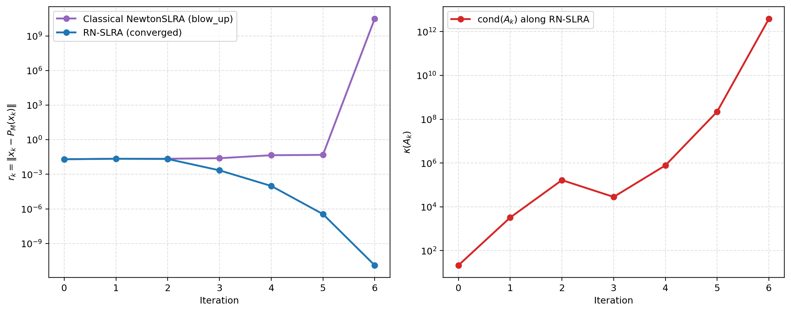
RN-SLRA converges in \(7\) steps, taking \(0.001852s\), while Newton-SLRA diverges. From the right plot, we can see that the condition number of matrix \(A\) becomes extremely large during the iteration process of RN-SLRA, while RN-SLRA still converges rapidly. This example illustrates the stabilizing effect of the regularization term in a nontransversal SLRA problem.
To further check that the above behavior is not caused by a single specially chosen initial point, we also perform a random initialization test on the same example. We generate \(x_0 = x^* + \alpha \sum_{i=1}^4 a_i B_i,\) where \(a=(a_1,\ldots,a_4)\) is obtained by sampling a standard Gaussian vector in \(\mathbb{R}^4\) and normalizing it to satisfy \(\|a\|_2=1\). The radius \(\alpha\) is sampled independently from the uniform distribution \(\alpha \sim U(0.01,0.1).\) We use \(1000\) random initial points. The parameters of RN-SLRA are kept the same as above. The success rates are reported in Table 2.
| Method | Successful runs | Success rate |
|---|---|---|
| Newton-SLRA | \(591/1000\) | \(59.1\%\) |
| RN-SLRA | \(1000/1000\) | \(100\%\) |
The result shows that Newton-SLRA is sensitive to the initialization in this nontransversal example, whereas RN-SLRA succeeds for all tested initial points. This supports the observation from Fig. 2 that the regularization stabilizes the Newton iteration near this degenerate intersection.
5.1.2 Example 2: linear convergence of RN-SLRA and comparison with Cadzow↩︎
In the previous example, we observed the superlinear convergence of RN-SLRA. We now construct an example for which RN-SLRA exhibits only linear local convergence. This shows that the theoretical linear convergence rate of RN-SLRA is, in general, not improvable. Moreover, using the same example, we compare RN-SLRA with the Cadzow algorithm and show that RN-SLRA can converge much faster, although both algorithms are linearly convergent.
Similar to the previous construction process, we take \(x^*=\operatorname{diag}(4,0.1,0,0),\) and \[\begin{cases} \widetilde{B}_1 = E_{13}+0.6E_{31}+1.0E_{33},& \widetilde{B}_2 = E_{24}-0.5E_{42}+1.0E_{33},\\ \widetilde{B}_3 = E_{34}+0.1E_{12}+0.2E_{44},& \widetilde{B}_4 = E_{43}-0.1E_{21}+0.6E_{44}+0.4E_{33}. \end{cases}\] The initial point is chosen as \(x_0=x^*+0.01\sum_{i=1}^4 a_i B_i,\) with \(a=(1,-1,0.5,0.2).\) We set the parameters of RN-SLRA to \(c=0.001\) and \(\rho=1\). On this example, RN-SLRA converges linearly in \(10\) steps, taking \(0.002545\)s, with an approximate convergence rate \(q=0.2501\).
We further compare the numerical performance of RN-SLRA and Cadzow on the same example with the same parameters. For both algorithms, the maximal number of iterations is set to \(1000\). The numerical results are presented in Table 3. The residual ratio is the median of the last five values of \(r_{k+1}/r_k\), with \(r_k=\|x_k-P_{D_r}(x_k)\|\).
| Method | Iter. | Time (s) | Final residual | Residual ratio |
|---|---|---|---|---|
| Cadzow | 1000(max) | 0.067744 | 1.03782e-4 | 0.9993 |
| RN-SLRA | 11 | 0.002545 | 6.78165e-11 | 0.2501 |
The results show that RN-SLRA converges much faster than Cadzow on this example. This behavior is consistent with the local geometry of the problem: alternating projections can be slow when the two sets meet with a very small effective angle, as in the simple case of two nearly parallel intersecting lines. Our constructed example exhibits a similar local geometry near the intersection point. Thus, this example illustrates that RN-SLRA may have only linear local convergence under nontransversality, but can still be much faster than Cadzow.
5.2 Large-scale SLRA Problems↩︎
We construct the intersection point \(x^*\) and the affine subspace \(E\) in large-scale experiments using a similar method as before, and choose the initial point as \(x_0=P_E(x^*+\alpha G)\), where \(G_{ij}\sim N(0,1)\) are i.i.d. We compare RN-SLRA and Cadzow in nine large-scale experiments; see Fig. 3, where \(n,m\) are the matrix dimensions, \(p=\dim E\), and \(r\) is the target rank. For each tuple \((n,m,p,r)\), both methods use the same initial point, with \(\alpha=0.05\) for the \(100\times100\) cases, \(\alpha=0.02\) for the larger cases, and stopping tolerance \(10^{-8}\).
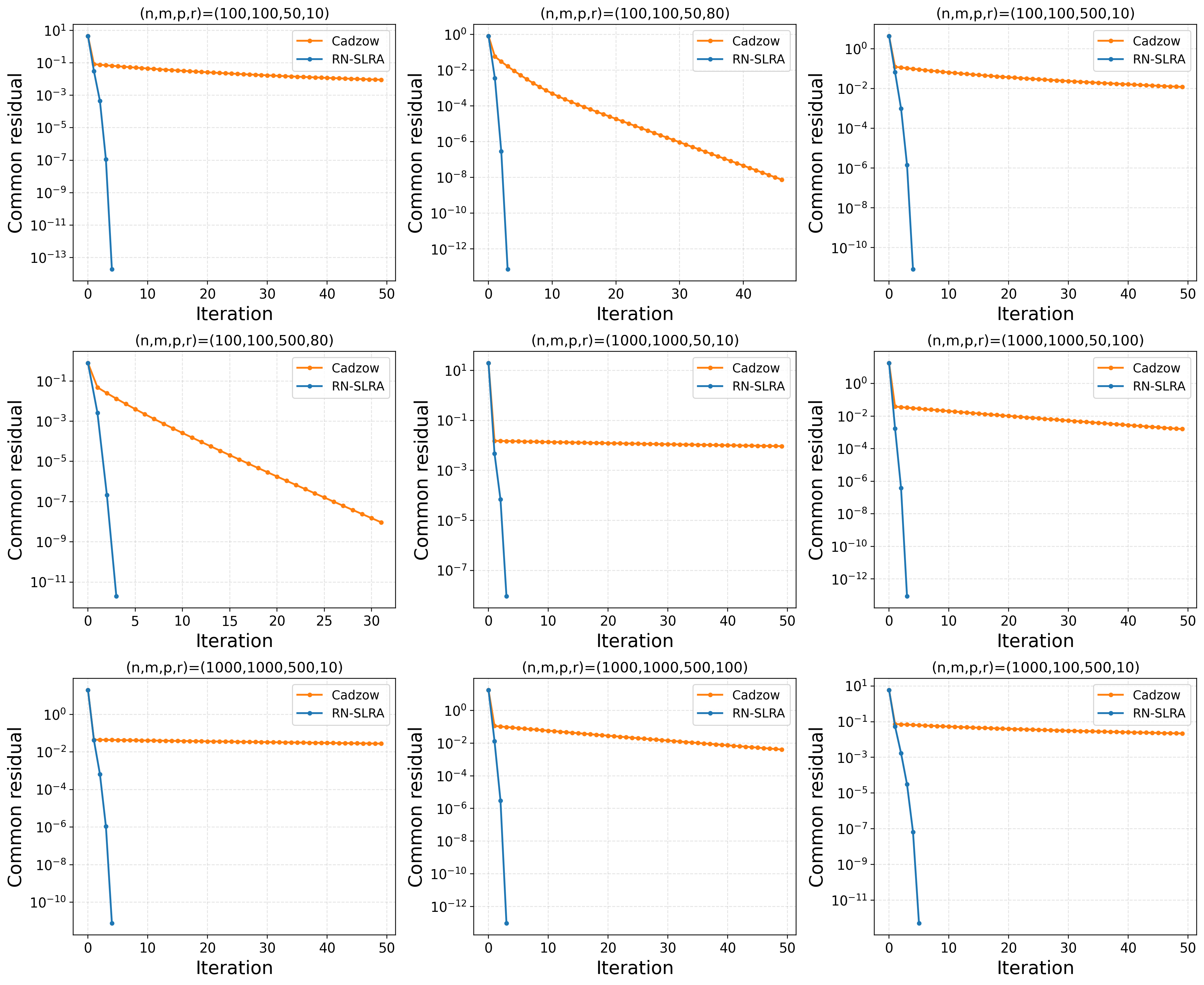
As shown in Fig. 3, RN-SLRA converges within five iterations in all cases, whereas Cadzow converges much more slowly.
5.3 Low-Rank Approximation of Hankel Matrices↩︎
We now test the performance of RN-SLRA for low-rank approximation of Hankel matrices [11]. We compare RN-SLRA with four representative baseline families for Hankel structured low-rank approximation: Cadzow; VP-SLRA, based on variable projection and reduced nonlinear optimization for affinely structured SLRA [15]; STLN, which approaches the problem from a structured error-correction perspective [10], [46]; and Gradient-system, based on low-rank factor updates with a Hankel penalty [16].
We will construct a single example and then perform both a noise sweep and an outlier sweep to compare RN-SLRA with the baselines on geometrically degenerate Hankel low-rank approximation problems.
5.3.1 Single example↩︎
We consider a \(7\times5\) rank-\(4\) Hankel matrix \(H_c=(\nu_{i+j-1})\), where \(\nu_i=\sum_{\ell=1}^4\beta_\ell z_\ell^i\) for \(i=1,\ldots,11\). Here \(\beta=(1.2,0.9,1.0,1.1)\) and \(z=(e^{-0.2},e^{-0.2+10^{-3}},e^{-0.35},e^{-0.5})\). The closeness of the first two poles makes the instance geometrically degenerate.
The perturbed initial matrix is generated as \[\begin{align} \label{eq:H0} H_0=H_c+\tau \Delta + \eta E_{\text{out}}, \end{align}\tag{40}\] where \(\Delta\) is a random Hankel noise matrix, \(E_{\text{out}}\) is a Hankel matrix supported on the 9-th anti-diagonal, and in this example we choose \(\tau=3\times 10^{-3},\eta=1\times10^{-2}\). \(\Delta\) is a Hankel matrix with generating entries picked independently from \(\mathcal{N}(0,1)\).
We set the parameter of RN-SLRA to \(c=1\times 10^{-7},\rho=1\). We terminate a algorithm if it is stalled or its iteration counts reach the maximal number 300. The numerical results are presented in Fig. 4.
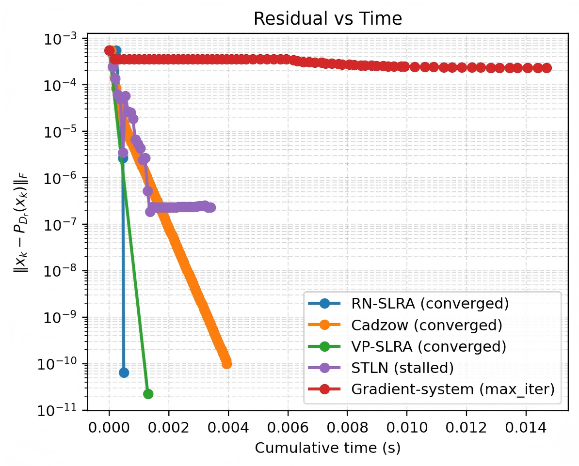
This result shows that RN-SLRA still converges within only a few iterations and rapidly reduces the residual to high accuracy. VP-SLRA also converges to a very small residual, but requires more CPU time than RN-SLRA. Cadzow converges more slowly, while STLN stalls at a moderate residual level, and the gradient-system method fails to make substantial progress within the prescribed maximum number of iterations. These results demonstrate that RN-SLRA remains effective for geometrically degenerate structured low-rank approximation problems, achieving fast convergence and competitive accuracy.
5.3.2 Noise Sweep and Outlier Sweep↩︎
We next test the robustness of RN-SLRA under different noise and outlier levels. In both sweeps, the initial point is generated by 40 , and several independent random Hankel noises \(\Delta\) are used. For the noise sweep, the outlier level \(\eta\) is fixed and \(\tau\in\{10^{-4},3\times10^{-4},10^{-3},3\times10^{-3}\}\). For the outlier sweep, the noise level \(\tau\) is fixed and \(\eta\in\{0,10^{-3},3\times10^{-3},10^{-2}\}\). The mean CPU times over 30 random perturbations are reported in Table 4. Here “fail” means that the algorithm either fails to converge within the prescribed iteration limit or stalls.
| Sweep | Level | RN | Cadzow | VP | STLN | GS |
|---|---|---|---|---|---|---|
| Noise | \(10^{-4}\) | \(0.0009\pm0.0003\) | \(0.0030\pm0.0014\) | \(0.0028\pm0.0023\) | fail | fail |
| Noise | \(3\cdot 10^{-4}\) | \(0.0009\pm0.0003\) | \(0.0031\pm0.0014\) | \(0.0016\pm0.0003\) | fail | fail |
| Noise | \(10^{-3}\) | \(0.0009\pm0.0004\) | \(0.0034\pm0.0015\) | \(0.0016\pm0.0004\) | fail | fail |
| Noise | \(3\cdot 10^{-3}\) | \(0.0008\pm0.0002\) | \(0.0039\pm0.0015\) | \(0.0016\pm0.0003\) | fail | fail |
| Outlier | \(0\) | \(0.0009\pm0.0003\) | \(0.0035\pm0.0013\) | \(0.0018\pm0.0005\) | fail | fail |
| Outlier | \(10^{-3}\) | \(0.0008\pm0.0001\) | \(0.0039\pm0.0018\) | \(0.0021\pm0.0013\) | fail | fail |
| Outlier | \(3\cdot 10^{-3}\) | \(0.0008\pm0.0002\) | \(0.0032\pm0.0017\) | \(0.0018\pm0.0002\) | fail | fail |
| Outlier | \(10^{-2}\) | \(0.0008\pm0.0002\) | \(0.0036\pm0.0018\) | \(0.0023\pm0.0009\) | fail | fail |
4pt
The results show that RN-SLRA remains robust and consistently achieves the smallest mean CPU time across both sweeps. VP-SLRA and Cadzow also converge, but require more time, while STLN and Gradient-system fail on all tested instances. This further illustrates the effectiveness of RN-SLRA on examples with poor geometry.
5.3.3 Large-scale inexact-projection experiment↩︎
We finally compare RN-SLRA with iRN-SLRA when the rank-\(r\) projection is computed only approximately. Here \(n\) and \(m\) denote the matrix dimensions and \(r\) is the target rank. We use larger degenerate Hankel SLRA instances \(H_c^{(n,m,3)}\in\mathbb{R}^{n\times m}\) generated from the repeated-pole model \(\nu_i=\beta_0\lambda^i+\beta_1 i\lambda^i+\beta_2\mu^i\), where the term \(i\lambda^i\) induces poor local geometry. We test \((n,m,r)\in\{(120,160,3),(200,280,3),(350,500,3),(700,1000,3)\}\).
To keep the instances comparable, the poles are moved closer to one as the matrix size increases and the coefficients are mildly rescaled. For these four sizes, the corresponding \((\lambda,\mu,\beta_0,\beta_1,\beta_2)\) are \((e^{-0.06},e^{-0.19},1.0,0.09,0.8)\), \((e^{-0.035},e^{-0.12},1.0,0.06,\) \(0.65)\), \((e^{-0.022},e^{-0.075},1.0,0.045,0.55)\), and \((e^{-0.012},e^{-0.045},1.0,0.025,0.45)\).
The initial matrix is \(H_0=H_c+\tau\Delta+\eta E_{\mathrm{out}}\), where \(\Delta\) is random Hankel noise and \(E_{\mathrm{out}}\) is a Hankel outlier supported on one anti-diagonal. We normalize the perturbations by \(\alpha_c=\|H_c\|/\sqrt{mn}\), and set \(\tau=5\times10^{-2}\alpha_c\), \(\eta=10^{-1}\alpha_c\). For both methods, we tune \(c\in\{10^{-8},3\times10^{-8},10^{-7},3\times10^{-7},10^{-6}\}\) and \(\rho\in\{0,0.5,1.0\}\). For iRN-SLRA, the rank-\(r\) projection is approximated by randomized SVD [38]. We use \(\varepsilon_{\rm r}\in\{0.1,0.25\}\) as the relative tolerance in the randomized SVD routine, and \(s\in\{1,2,3\}\) as the number of subspace iterations. The stopping tolerance is \(10^{-7}\), and the maximum number of outer iterations is \(40\).
| \((n,m,r)\) | RN-SLRA | iRN-SLRA | ||||
| Iter. | Time (s) | Final residual | Iter. | Time (s) | Final residual | |
| (120,160,3) | 6 | 0.8515 | \(2.62{\times}10^{-10}\) | 4 | 0.4793 | \(5.60{\times}10^{-10}\) |
| (200,280,3) | 7 | 2.8913 | \(1.63{\times}10^{-10}\) | 4 | 1.3842 | \(3.82{\times}10^{-10}\) |
| (350,500,3) | 5 | 9.3378 | \(1.33{\times}10^{-10}\) | 4 | 6.8277 | \(3.68{\times}10^{-13}\) |
| (700,1000,3) | 6 | 98.1399 | \(2.33{\times}10^{-10}\) | 4 | 58.0918 | \(5.74{\times}10^{-10}\) |
Table 5 shows that iRN-SLRA preserves the robustness of RN-SLRA while reducing the running time. The gain becomes more pronounced at larger scales; for \((700,1000,3)\), the time decreases from \(98.14\) to \(58.09\) seconds.
6 Conclusion↩︎
We proposed RN-SLRA, a regularized Newton-type method for local manifold–affine intersection problems. The method is well defined under intrinsic transversality, where we proved local linear convergence, and achieves order \(1+\rho\) under transversality with \(\mu_k=c r_k^\rho\), including quadratic convergence when \(\rho=1\). We also developed an inexact variant, iRN-SLRA, and showed that the same local rates are preserved under a suitable quasioptimal projection condition. Numerical experiments illustrate the robustness of RN-SLRA and the efficiency of iRN-SLRA.
7 Numerical Diagnostics of Intrinsic Transversality↩︎
This appendix reports numerical diagnostics supporting the intrinsic transversality condition in the examples used in the numerical experiments.
7.1 Numerical Principle↩︎
Let \(E\) be the affine constraint set and let \(D_r\) be the fixed-rank manifold of rank-\(r\) matrices. Around a point \(x^*\in E\cap D_r\), we sample nearby points \(x\in E\) and \(y\in D_r\), and define \[u=\frac{x-y}{\|x-y\|_F}.\] We then compute the intrinsic transversality proxy \[\eta(x,y) = \max\Big\{ \operatorname{dist}\big(u,N_{D_r}(y)\big), \operatorname{dist}\big(u,N_E(x)\big) \Big\}.\] Since \(E\) is affine, \(N_E(x)\) is independent of \(x\). A positive lower bound on \(\eta(x,y)\) over nearby sampled pairs indicates that the displacement direction cannot be simultaneously close to both normal geometries, which is the separation expected from intrinsic transversality.
For the small synthetic examples, we also report the singular values of the classical tangent-intersection matrix \(A(x^*)\). A zero or nearly zero smallest singular value indicates failure of classical transversality, whereas positive sampled values of \(\eta\) support the weaker intrinsic transversality condition used in this paper.
7.2 Example 1: Newton-SLRA versus RN-SLRA↩︎
For the first synthetic example, the singular values of the classical tangent-intersection matrix at the solution are \[\sigma(A(x^*)) = (0.9950,\;0.9806,\;0.7645,\;0).\] Thus the classical transversality matrix is rank deficient. Nearby random rank-\(2\) points nevertheless yield positive sampled smallest singular values: \[\begin{array}{c|ccc} \hline \text{sampling scale} & \min \sigma_{\min} & \operatorname{median}\sigma_{\min} & \max \sigma_{\min}\\ \hline 10^{-3} & 5.1222\cdot 10^{-8} & 2.7545\cdot 10^{-6} & 5.0001\cdot 10^{-5}\\ 10^{-2} & 1.2180\cdot 10^{-4} & 3.3858\cdot 10^{-3} & 5.4935\cdot 10^{-2}\\ 5\cdot 10^{-2} & 3.3860\cdot 10^{-5} & 7.0428\cdot 10^{-3} & 1.4893\cdot 10^{-1}\\ \hline \end{array}\]
The intrinsic transversality proxy was then computed for nearby pairs \(x\in E\) and \(y\in D_2\): \[\begin{array}{ccccc} \hline \text{scale}_x & \text{scale}_y & \text{samples} & \min \eta & \operatorname{median}\eta\\ \hline 0.01 & 0.01 & 200 & 0.6611 & 0.9306\\ 0.01 & 0.02 & 200 & 0.8828 & 0.9787\\ 0.01 & 0.05 & 142 & 0.9683 & 0.9937\\ 0.02 & 0.01 & 200 & 0.6706 & 0.8783\\ 0.02 & 0.02 & 200 & 0.7721 & 0.9510\\ 0.02 & 0.05 & 144 & 0.8753 & 0.9896\\ 0.05 & 0.01 & 200 & 0.7323 & 0.9428\\ 0.05 & 0.02 & 200 & 0.7363 & 0.9105\\ 0.05 & 0.05 & 145 & 0.7489 & 0.9585\\ \hline \end{array}\] All sampled minima are bounded away from zero.
7.3 Random Initializations for Example 1↩︎
The random-initialization experiment uses the same affine-rank geometry as Example 1 and changes only the initial point distribution. The intrinsic transversality diagnostics are therefore the same as those reported above.
7.4 Linear-Convergence Example↩︎
For the selected linear-convergence example, the tangent-intersection singular values at \(x^*\) are \[\sigma(A(x^*)) = (0.9968,\;0.9951,\;0.7604,\;9.2694\cdot 10^{-21}),\] so classical transversality again fails numerically. The intrinsic proxy was sampled at scale \(0.02\) with 80 random pairs, giving \[\min \eta = 0.7482.\] This positive value supports intrinsic transversality for this example.
7.5 Cadzow versus RN-SLRA on the Linear-Convergence Example↩︎
The Cadzow comparison uses the same geometry as the linear-convergence example. Hence the corresponding diagnostics are \[\sigma(A(x^*)) = (0.9968,\;0.9951,\;0.7604,\;9.2694\cdot 10^{-21}), \qquad \min \eta = 0.7482.\]
7.6 Large-Scale Synthetic SLRA Examples↩︎
For the nine large-scale synthetic SLRA examples, we report a rank bound for the classical transversality matrix and the minimum sampled intrinsic proxy. The proxy is computed over 24 local samples with sampling radius \(0.01\).
\[\begin{array}{ccccc} \hline (m,n) & p & r & \text{rank bound} & \min \eta\\ \hline (100,100) & 50 & 10 & 2 & 0.9998316\\ (100,100) & 50 & 80 & 2 & 0.9997508\\ (100,100) & 500 & 10 & 2 & 0.9995969\\ (100,100) & 500 & 80 & 2 & 0.9995995\\ (1000,1000) & 50 & 10 & 2 & 0.9999997\\ (1000,1000) & 50 & 100 & 2 & 0.9999983\\ (1000,1000) & 500 & 10 & 2 & 0.9999981\\ (1000,1000) & 500 & 100 & 2 & 0.9999890\\ (1000,100) & 500 & 10 & 2 & 0.9999526\\ \hline \end{array}\]
In all nine cases, the sampled intrinsic proxy is close to one. In contrast, the recorded transversality rank bound is \(2\), much smaller than the number of affine constraints \(p\). This is consistent with the construction: the examples are rank deficient in the classical tangent-intersection sense, while retaining a strong sampled intrinsic separation.
7.7 Hankel SLRA Experiments↩︎
We also computed the intrinsic transversality proxy for the small Hankel experiments. For each case, 200 sampled pairs were used at each radius \(\rho\in\{0.01,0.02,0.05\}\). The table reports the smallest sampled value of \(\eta\) over these radii, together with the range of median values. The column \(\sigma_{\min}(A)\) gives the smallest singular value of the tangent-restriction matrix when it was explicitly formed.
\[\begin{array}{lccccc} \hline \text{experiment} & (m,n) & r & \sigma_{\min}(A) & \min \eta & \operatorname{median}\eta\text{ range}\\ \hline \text{single example} & (7,5) & 4 & 4.5647\cdot 10^{-1} & 0.8628 & [0.9788,0.9800]\\ \text{noise sweep} & (7,5) & 4 & 4.5575\cdot 10^{-1} & 0.8234 & [0.9783,0.9788]\\ \text{noise sweep} & (7,5) & 4 & 4.5647\cdot 10^{-1} & 0.8710 & [0.9788,0.9802]\\ \text{noise sweep} & (8,5) & 2 & 4.8981\cdot 10^{-17} & 0.7718 & [0.8812,0.8838]\\ \text{outlier sweep} & (7,5) & 4 & 4.5575\cdot 10^{-1} & 0.8864 & [0.9803,0.9815]\\ \text{outlier sweep} & (7,5) & 4 & 4.5647\cdot 10^{-1} & 0.8391 & [0.9778,0.9799]\\ \text{outlier sweep} & (8,5) & 2 & 4.8981\cdot 10^{-17} & 0.7627 & [0.8761,0.8792]\\ \hline \end{array}\]
For all small Hankel cases, the sampled intrinsic proxy remains bounded away from zero. Some cases have a nearly singular tangent-restriction matrix, while their intrinsic proxy remains positive. This is consistent with the pattern observed in the synthetic SLRA examples.
7.8 Large-Scale Hankel Intrinsic Diagnostics↩︎
For the large-scale Hankel benchmark used in Table 5, the tangent-restriction matrix was not explicitly formed. The intrinsic proxy was computed directly from sampled normal-cone distances, using 24 sampled pairs at radius \(0.01\) for each case.
\[\begin{array}{ccccc} \hline (m,n) & r & \text{samples} & \min\eta & \operatorname{median}\eta\\ \hline (160,120) & 3 & 24 & 0.9752 & 0.9786\\ (280,200) & 3 & 24 & 0.9852 & 0.9879\\ (500,350) & 3 & 24 & 0.9920 & 0.9927\\ (1000,700) & 3 & 24 & 0.9961 & 0.9964\\ \hline \end{array}\] All four large-scale Hankel cases have sampled \(\eta\)-values close to one, providing further numerical evidence of intrinsic separation.
8 Retraction induced by RN-SLRA in the case \(\rho=0\)↩︎
In this appendix we justify the retraction interpretation in Remark [rmk:retraction-clean-intersection] for the special case \(\rho=0\). In this case the residual-dependent rule \(\mu_k=c r_k^\rho\) is understood as the fixed choice \(\mu_k\equiv c>0\).
Let \(\Phi_c:E\to E\) denote the one-step RN-SLRA map with \(\mu_k\equiv c\). For \(z\in E\) close to \(X\), set \(y=P_M(z)\), \(Q_y:=P_{N_yM}\), and define \[\Phi_c(z) := \arg\min_{u\in E} \left\{ \frac{1}{2}\|u-y\|^2 + \frac{1}{2c}\|Q_y(u-y)\|^2 \right\}.\] We first show that, under clean intersection and suitable smoothness, the limiting map of \(\Phi_c\) defines a genuine retraction on \(X\). We then show that one additional order of smoothness yields a second-order retraction.
Theorem 8 (Retraction for RN-SLRA when \(\rho=0\)). Assume that \(E\) intersects \(M\) cleanly at \(\bar x\). Assume further that the fixed-regularization one-step map \(\Phi_c\) is of class \(C^2\) in a neighborhood of \(X\); for instance, this holds if \(M\) is locally \(C^3\) near \(\bar x\). Then, for all \(z\in E\) sufficiently close to \(X\), the limit \[\Psi_c(z):=\lim_{k\to\infty}\Phi_c^k(z)\] exists locally and \(\Psi_c\) is \(C^1\). Consequently, \[R_x^c(\xi):=\Psi_c(x+\xi), \qquad x\in X,\quad \xi\in T_xX,\] defines a \(C^1\) retraction on \(X\).
Proof. For \(y\) close to \(X\), write \(p=P_E(y)\). Since every point in \(E\) can be written as \(p+\ell\) with \(\ell\in L\), the subproblem defining \(\Phi_c(z)\) is equivalent to minimizing over \(\ell\in L\). Its first-order optimality condition is \[\ell+\frac{1}{c} P_LQ_y(p-y+\ell)=0 .\] Equivalently, \[(cI_L+A_y)\ell=-P_LQ_y(p-y), \qquad A_y:=P_LQ_y|_L .\] Since \(A_y\) is self-adjoint positive semidefinite on \(L\) and \(c>0\), the operator \(cI_L+A_y\) is uniformly invertible. Hence \(\Phi_c\) is locally well defined and inherits the assumed smoothness.
For \(x\in X\), we have \(P_M(x)=x\), \(P_E(x)=x\), and hence \(\Phi_c(x)=x\). Thus \(X\) is a fixed-point manifold of \(\Phi_c\). We now compute the derivative of \(\Phi_c\) at \(x\in X\). Let \(h\in L\). Since \(\mathrm{D}P_M(x)h=P_{T_xM}h\), differentiating the optimality system at \(x\) gives \[(cI_L+A_x)\ell' = -P_LQ_x\big(P_LP_{T_xM}h-P_{T_xM}h\big), \qquad A_x:=P_LQ_x|_L .\] Using \(P_{T_xM}=I-Q_x\) and \(h\in L\), we have \(P_LP_{T_xM}h=h-A_xh\). Hence the right-hand side equals \(-A_x(I_L-A_x)h\), and therefore \[\ell'=-(cI_L+A_x)^{-1}A_x(I_L-A_x)h .\] Since \(\mathrm{D}\Phi_c(x)h=P_LP_{T_xM}h+\ell'\), we obtain \[\label{eq:rho0-DPhi} \mathrm{D}\Phi_c(x)h = \left(I_L+c^{-1}A_x\right)^{-1}(I_L-A_x)h .\tag{41}\]
The operator \(A_x\) is self-adjoint and positive semidefinite on \(L\), because \[\langle A_xh,h\rangle = \langle Q_xh,h\rangle = \|Q_xh\|^2 .\] Moreover, \[\ker A_x = \{h\in L:Q_xh=0\} = L\cap T_xM = T_xX,\] where the last equality follows from clean intersection. Let \(W_x:=L\ominus T_xX\). Since \(A_x\) depends continuously on \(x\) and \(\dim T_xX\) is locally constant under clean intersection, the nonzero eigenvalues of \(A_x\) are locally bounded away from zero. Hence, after shrinking the neighborhood if necessary, there exists \(\sigma>0\) such that \[\label{eq:rho0-uniform-positive} \langle A_xh,h\rangle\ge \sigma\|h\|^2, \qquad h\in W_x,\quad x\in X .\tag{42}\] Thus \(\mathrm{D}\Phi_c(x)h=h\) for \(h\in T_xX\). If \(h\in W_x\) is an eigenvector of \(A_x\) with eigenvalue \(\lambda\in[\sigma,1]\), then \[\mathrm{D}\Phi_c(x)h = \frac{1-\lambda}{1+\lambda/c}h .\] Consequently, the derivative is the identity along \(T_xX\) and is uniformly contractive on \(W_x\). Therefore \(X\) is a normally attracting fixed-point manifold of \(\Phi_c\).
We next prove the \(C^1\) regularity of the limiting map. We work in a local tubular coordinate system in \(E\) around \(X\). Namely, for \(z\in E\) close to \(X\), write \[z=s+w,\qquad s=P_X(z),\qquad w\in W_s:=L\ominus T_sX .\] Using a smooth local frame of the bundle \(W_s\), we identify the spaces \(W_s\) with a fixed Euclidean space. In these coordinates, write \[\Phi_c(s,w)=\big(s+a(s,w),\,B_s w+b(s,w)\big).\] Since every point of \(X\) is fixed by \(\Phi_c\), and since the derivative of \(\Phi_c\) is the identity in the tangent direction and has no first-order tangential response in the normal direction, we have \[a(s,0)=0,\qquad b(s,0)=0,\qquad D_w a(s,0)=0,\qquad D_w b(s,0)=0.\] Moreover, by the uniform contraction on \(W_s\), after shrinking the neighborhood if necessary, \[\|B_s\|\le q<1\] uniformly for \(s\in X\) close to \(\bar x\). Since \(\Phi_c\) is \(C^2\), it follows that \[\label{eq:rho0-ab-quadratic} a(s,w)=O(\|w\|^2), \qquad b(s,w)=O(\|w\|^2).\tag{43}\] Moreover, \[\label{eq:rho0-first-derivative-estimates} \begin{align} D_s a(s,w)&=O(\|w\|),& D_w a(s,w)&=O(\|w\|),\\ D_s b(s,w)&=O(\|w\|),& D_w b(s,w)&=O(\|w\|). \end{align}\tag{44}\] All estimates are local and uniform.
Let \[(s_{k+1},w_{k+1})=\Phi_c(s_k,w_k), \qquad (s_0,w_0)=(s,w).\] The normal component satisfies \[w_{k+1}=B_{s_k}w_k+b(s_k,w_k).\] Choose \(\theta\in(q,1)\). By 43 , after shrinking the neighborhood if necessary, the nonlinear term \(b(s,w)\) is small enough so that \[\label{eq:rho0-normal-decay} \|w_k\|\le C\theta^k\|w_0\|.\tag{45}\] Moreover, \[s_{k+1}-s_k=a(s_k,w_k),\] and hence, by 43 and 45 , \[\sum_{k=0}^{\infty}\|s_{k+1}-s_k\| \le C\sum_{k=0}^{\infty}\|w_k\|^2 \le C\|w_0\|^2.\] Therefore \(s_k\) converges to a limit \(s_\infty\), \(w_k\to0\), and \[\label{eq:rho0-limit-representation} \Psi_c(s,w)=(s_\infty,0), \qquad s_\infty=s+\sum_{k=0}^{\infty}a(s_k,w_k).\tag{46}\]
It remains to justify the \(C^1\) dependence on the initial point. Differentiating the recursions and using 44 , 45 , and the uniform contraction in the \(w\)-equation gives, by a standard induction on the differentiated recursions, \[\label{eq:rho0-first-derivative-bounds} \|D_z w_k\|\le C\theta^k, \qquad \sup_k\|D_z s_k\|\le C .\tag{47}\] By the chain rule and 44 , \[\begin{align} \|D_z a(s_k,w_k)\| &\le C\|w_k\|\big(\|D_zs_k\|+\|D_zw_k\|\big) \\ &\le C'\theta^k . \end{align}\] Thus the derivative series \[D_zs_0+\sum_{k\ge0}D_z a(s_k,w_k)\] converges uniformly. It follows from 46 that \(s_\infty\) is \(C^1\), and therefore \(\Psi_c(s,w)=(s_\infty(s,w),0)\) is \(C^1\).
Finally, define, for \(x\in X\) close to \(\bar x\) and \(\xi\in T_xX\) sufficiently small, \[R_x^c(\xi):=\Psi_c(x+\xi).\] Since \(\Psi_c\) is \(C^1\), \(R^c:TX\to X\) is \(C^1\). Also, \(\Psi_c(x)=x\) for every \(x\in X\). Hence, for any \(\xi\in T_xX\), taking a \(C^1\) curve \(\gamma(t)\subset X\) with \(\gamma(0)=x\) and \(\gamma'(0)=\xi\), we have \(\Psi_c(\gamma(t))=\gamma(t)\), and therefore \(\mathrm{D}\Psi_c(x)\xi=\xi\). Consequently, \[R_x^c(0_x)=x, \qquad \mathrm{D}R_x^c(0_x)=\mathrm{id}_{T_xX}.\] Thus \(R^c\) is a \(C^1\) retraction on \(X\). ◻
Theorem 9 (Second-order retraction for RN-SLRA when \(\rho=0\)). Assume the hypotheses of Theorem 8. Assume in addition that the fixed-regularization one-step map \(\Phi_c\) is of class \(C^3\) in a neighborhood of \(X\); for instance, this holds if \(M\) is locally \(C^4\) near \(\bar x\). Then the limiting map \(\Psi_c\) is \(C^2\). Consequently, \[R_x^c(\xi):=\Psi_c(x+\xi), \qquad x\in X,\quad \xi\in T_xX,\] defines a second-order retraction on \(X\).
Proof. We use the notation and local coordinates from the proof of Theorem 8. Since now \(\Phi_c\) is \(C^3\), the functions \(a\) and \(b\) satisfy the following strengthened local estimates. Indeed, the fixed-point property on \(X\) gives \(a(s,0)=b(s,0)=0\), and the normal-form construction gives \(D_w a(s,0)=D_w b(s,0)=0\). Hence, by Taylor’s formula in the normal variable \(w\), uniformly for \(s\) near \(\bar x\), \[a(s,w)=O(\|w\|^2),\qquad b(s,w)=O(\|w\|^2),\] and, differentiating this Taylor representation with respect to \(s\) and \(w\), \[\label{eq:rho0-strong-first-derivative-estimates} \begin{align} D_s a(s,w)&=O(\|w\|^2),& D_w a(s,w)&=O(\|w\|),\\ D_s b(s,w)&=O(\|w\|^2),& D_w b(s,w)&=O(\|w\|), \end{align}\tag{48}\] and, for the second derivatives, \[\label{eq:rho0-second-derivative-estimates} \begin{align} D_s^2a(s,w)&=O(\|w\|),& D_sD_w a(s,w)&=O(\|w\|),& D_w^2a(s,w)&=O(1),\\ D_s^2b(s,w)&=O(\|w\|),& D_sD_w b(s,w)&=O(\|w\|),& D_w^2b(s,w)&=O(1). \end{align}\tag{49}\] All estimates are local and uniform. The weaker \(O(\|w\|)\) estimate for \(D_s^2a\) and \(D_s^2b\) is sufficient for the argument below.
We already know from the proof of Theorem 8 that \[\label{eq:rho0-basic-bounds} \|w_k\|\le C\theta^k\|w_0\|, \qquad \|D_z w_k\|\le C\theta^k, \qquad \sup_k\|D_zs_k\|\le C.\tag{50}\] We now control the second derivatives. Differentiating the recursions twice, and using 48 –50 , yields inequalities of the form \[\begin{align} \|D_z^2 w_{k+1}\| &\le q\|D_z^2 w_k\| + C\theta^k \bigl(1+\|D_z^2s_k\|+\|D_z^2w_k\|\bigr), \tag{51}\\ \|D_z^2 s_{k+1}\| &\le \|D_z^2 s_k\| + C\theta^k\|D_z^2w_k\| + C\theta^{2k}\bigl(1+\|D_z^2s_k\|\bigr). \tag{52} \end{align}\] Indeed, 51 follows from the normal recursion \(w_{k+1}=B_{s_k}w_k+b(s_k,w_k)\): the leading term is \(B_{s_k}D_z^2w_k\), while all remaining terms contain either a factor \(w_k\), \(D_z w_k\), or a coefficient of order \(O(\|w_k\|)\). The estimate 52 is obtained similarly from the tangential recursion \(s_{k+1}=s_k+a(s_k,w_k)\). By 51 , since \(q<\theta<1\), a discrete Gronwall argument gives \[\|D_z^2w_k\| \le C\theta^k \left(1+\sup_{0\le j\le k}\|D_z^2s_j\|\right).\] Substituting this estimate into 52 , we obtain \[1+\sup_{0\le j\le k+1}\|D_z^2s_j\| \le \left(1+C\theta^{2k}\right) \left(1+\sup_{0\le j\le k}\|D_z^2s_j\|\right).\] Since \(\sum_{k=0}^\infty \theta^{2k}<\infty\), another discrete Gronwall argument yields \[\label{eq:rho0-second-derivative-bounds} \|D_z^2w_k\|\le C\theta^k, \qquad \sup_k\|D_z^2s_k\|\le C .\tag{53}\]
We next show that the second derivative series of \(s_\infty\) converges uniformly. By the chain rule, \[\begin{align} D_z^2(a(s_k,w_k)) &= D^2a(s_k,w_k) [D_z(s_k,w_k),D_z(s_k,w_k)] \\ &\quad + Da(s_k,w_k)D_z^2(s_k,w_k). \end{align}\] Using 48 –53 , each term on the right-hand side is bounded by \(C\theta^k\). Hence \[\|D_z^2(a(s_k,w_k))\|\le C\theta^k,\] and therefore \[\sum_{k=0}^{\infty}D_z^2(a(s_k,w_k))\] converges uniformly. The first derivative series already converges uniformly by Theorem 8. Thus \[s_\infty(s,w) = s+\sum_{k=0}^{\infty}a(s_k,w_k)\] is \(C^2\), and consequently \(\Psi_c(s,w)=(s_\infty(s,w),0)\) is \(C^2\).
It remains to verify the second-order retraction property. From 43 , 45 , and 46 , we have \[s_\infty-s = \sum_{k=0}^{\infty}a(s_k,w_k) = O(\|w_0\|^2).\] Since \(s=P_X(z)\) and \(\|w_0\|=\operatorname{dist}(z,X)\), this gives \[\label{eq:rho0-projection-second-order} \Psi_c(z)=P_X(z)+O(\operatorname{dist}(z,X)^2).\tag{54}\] Now take \(z=x+\xi\) with \(x\in X\) and \(\xi\in T_xX\). Since the intersection is clean and \(M\) is locally \(C^4\), the set \(X=M\cap E\) is a \(C^4\) embedded submanifold near \(\bar x\). Hence \[\operatorname{dist}(x+\xi,X)=O(\|\xi\|^2),\] and the metric projection retraction satisfies the standard expansion \[P_X(x+\xi) = \operatorname{Exp}_x(\xi)+O(\|\xi\|^3).\] Combining this with 54 , we obtain \[R_x^c(\xi) = \Psi_c(x+\xi) = P_X(x+\xi)+O(\|\xi\|^4) = \operatorname{Exp}_x(\xi)+O(\|\xi\|^3).\] Since \(R^c\) is \(C^2\), this proves that \(R^c\) is a second-order retraction on \(X\). ◻
References↩︎
School of Mathematical Sciences, Key Laboratory of the Ministry of Education for Mathematical Foundations and Applications of Digital Technology, University of Science and Technology of China, Hefei, Anhui, China (, ).↩︎
Our Python code is available at https://github.com/reniusll/Regularized-Newton-SLRA↩︎