A Quantum Collocation Approach to One-Dimensional Boundary Value Problems with Coherent Amplitude Amplification
June 30, 2026
Abstract
We propose a quantum collocation framework for approximating solutions of one-dimensional linear and nonlinear boundary value problems. The method formulates the search for admissible solutions as a residual-based quantum search over a discretized ansatz space, where candidate solutions are evaluated through residual conditions imposed at collocation points.
A residual-threshold oracle is constructed that acts jointly on spatial and parameter registers. This joint oracle structure leads to amplification dynamics that decompose into a coherent superposition of spatially conditioned amplitude-amplification processes rather than a single global amplification mechanism.
We derive the corresponding amplification geometry and show that the success probability is governed by a weighted combination of spatially dependent amplification angles. Furthermore, we prove that the reversible residual oracle can be implemented with gate complexity polynomial in the logarithm of the number of collocation points, while retaining the quadratic search acceleration associated with amplitude amplification in the parameter space.
We analyze how the spatially dependent oracle structure influences the amplification dynamics and corresponding success probabilities. Furthermore, we investigate how discretization, ansatz expressivity, oracle tolerance, and finite-precision effects influence both approximation quality and amplification behavior. Numerical experiments validate the theoretical predictions and illustrate the resulting search dynamics across different discretization and precision regimes.
\(^{1}\) Institute of Mathematics, Goethe University Frankfurt, Germany \(^{2}\) FCE Frankfurt Consulting Engineers GmbH, Frankfurt am Main, Germany
1 Introduction↩︎
Boundary value problems (BVPs) for ordinary differential equations (ODEs) arise throughout applied mathematics, physics, and engineering. Classical numerical approaches such as shooting methods, finite-difference schemes, finite-element methods, and spectral discretizations provide well-established tools for solving such problems [1]–[5]. In shooting methods, each residual evaluation requires solving an initial-value problem, with cost typically growing linearly with the number of integration steps. Finite-difference, finite-element, and spectral methods instead lead to algebraic systems whose cost depends on the number of degrees of freedom and the solver, ranging from linear to superlinear.
Quantum algorithms for differential equations have often been developed around quantum linear-system algorithms (QLSAs), in which a discretized differential equation is reduced to a linearsystem and the solution is encoded in a quantum state. Foundational examples include the HHL algorithm [6] and later improvements by Childs, Kothari, and Somma [7]. QLSA-based approaches have also been developed for finite-element discretizations and elliptic partial differential equations [8], [9].
Another direction uses Hamiltonian simulation or dynamical embeddings to represent differential equations as quantum dynamics. This includes quantum spectral methods [10], Schrödingerisation techniques [11], [12], and Hamiltonian-simulation-based solvers for partial differential equations [13]. For nonlinear differential equations, quantum algorithms based on Carleman linearization and Koopman-type embeddings have also been developed [14]–[16].
More recently, physics-informed neural networks (PINNs) have provided a residual-based framework for approximating solutions of differential equations [17]–[19]. Related quantum and hybrid quantum–classical approaches replace or augment the classical neural network by a parameterized quantum circuit [20], [21]. These methods retain the residual-minimization principle of PINNs and typically train the circuit parameters using a classical optimization procedure.
In this work, we pursue a different approach based on collocation and quantum amplitude amplification. Instead of solving a discretized linear system or simulating a dynamical evolution problem, we formulatethe solution process as a residual-driven quantum search problem over a discretized ansatz space. Candidate solutions are evaluated through residual conditions imposed at collocation points, and amplitudeamplification is used to enhance parameter configurations satisfying a prescribed residual tolerance.
A central feature of the proposed framework is that residual evaluation is performed coherently across both the collocation grid and the parameter space. This distinguishes the construction from a conventional Grover search in which each parameter configuration receives a single binary label. Instead, the oracle response reflects how the residual criterion is distributed across the spatial domain. Consequently, the amplification process retains information about where a candidate approximation satisfies or violates the differential equation.
The numerical behavior of the method is governed by the collocation grid, ansatz expressivity, residual tolerance, and arithmetic precision. These factors determine both the attainable approximation accuracy andthe oracle structure seen by amplitude amplification. We analyze their influence theoretically and through numerical experiments.
The remainder of the paper is organized as follows. Section 2 introduces the mathematical formulation of this special boundary value problem. Section 3 summarizes the main contributions of this work. Section 4 develops the quantum collocation method, including the reversible residual oracle andthe associated amplification dynamics. Section 5 analyzes the oracle complexity and compares the resulting runtime behavior with standard Grover amplification. Section 6 and 7 present numerical experiments and implementation studies illustrating the influence of discretization, oracle tolerance, finite precision, and ansatz expressivity on the search dynamics. Finally, we conclude the paper in Section 8.
2 Problem Formulation↩︎
We consider boundary value problems (BVPs) of the form \[u''(x) + f(x,u(x)) = 0, \quad x \in [0,1],\] subject to homogeneous boundary conditions \[u(0) = u(1) = 0.\] Here, \(f : [0,1] \times \mathbb{R} \to \mathbb{R}\) is a given (possibly nonlinear) function. The objective is to determine a function \(u^\ast : [0,1] \to \mathbb{R}\) that satisfies the differential equation together with the boundary conditions.
In general, closed-form solutions are not available, and one must resort to numerical approximation. In this work, we adopt a collocation-based perspective. Rather than solving the differential equation directly, we seek an approximate solution within a parametrized ansatz class of the form \(u(x,w)\), where \(w \in W_m\) denotes a finite-dimensional parameter vector.
To quantify how well a candidate function satisfies the differential equation, we introduce the residual function \[r(x,w) := u''(x,w) + f\bigl(x,u(x,w)\bigr),\] which measures the local deviation from the governing equation at a point \(x\).
The boundary value problem can then be reformulated as the task of identifying parameters \(w\) such that the residual is sufficiently small over the domain while the boundary conditionsare satisfied. In practice, this condition is enforced on a finite set of collocation points, leading to a discrete approximation of the continuous problem.
This formulation provides the basis for the quantum collocation method developed in the following sections.
3 Main Results↩︎
The main contributions of this work are summarized as follows.
We formulate one-dimensional boundary value problems as residual-based quantum search problems over discretized parameter spaces and construct a reversible residual-threshold oracle (Definition 1) acting jointly on spatial and parameter registers. Definition 2 and Lemma 1 show that the resulting oracle induces weighted rather than binary amplification, where the response of a parameter configuration \(w_j\) depends on the fraction of collocation points satisfying the residual threshold condition.
Theorem 1 shows that the amplification dynamics decompose into a coherent superposition of spatially conditionedamplitude amplification rotations, rather than a single global amplification process. This provides a natural extension of the standard amplitude amplification perspective tospatially conditioned oracle responses, while preserving compatibility with the usual quadratic search mechanism in the parameter space. The resulting success probability is governed by the spatial distribution of the local oracle responses.
Theorem 3 shows that, under a reversible implementation of the residual evaluation, the elementary gate complexity of the residual oracle scales polynomially in the spatial register size \(n_X=\log_2(N_X),\) rather than by an explicit linear enumeration of the \(N_X\) collocation points. Thus, one source of efficiency is the coherent evaluation of the residual over the spatial register. In the limiting case where the spatial dependence reduces to a standard binary marking of the parameterregister, Corollary 1 recovers the usual Grover scaling.
Numerical experiments validate the theoretical amplification behavior and illustrate the influence of discretization, oracle tolerance, finite-precision effects, and ansatz expressivity on the residual-based search dynamics.
4 Quantum Collocation Method↩︎
This section develops the quantum implementation of the residual-based collocation framework. We first introduce the register encodingsused to represent spatial points, parameters, and residual values. We then construct the residual-threshold oracle in compute–phase–uncompute form and analyze the induced amplification geometry.
The construction is organized around the fact that the residual test is evaluated on pairs \((x_i,w_j)\). This joint dependence determines the oracle structure and is the source of the spatially conditioned amplification behavior derived below.
4.1 Quantum Registers and Encodings↩︎
We use a state register \(X\), a parameter register \(W\), and asigned value register \(Z\). Their computational basis states encode, respectively, collocation points \(x_i\in X\), discretized parameter vectors \(w_j\in W_m\), and fixed-point values \(z_k\in Z\): \[\ket{i}_X \leftrightarrow x_i, \qquad \ket{j}_W \leftrightarrow w_j, \qquad \ket{k}_Z \leftrightarrow z_k.\] The signed value encoding is used to store residuals and intermediate arithmetic results and, in particular, permits operations conditioned on the sign of the encoded value.
Reversible arithmetic may additionally use an \(n_A\)-qubit ancilla register \(A\). The full computational Hilbert space is \[\mathcal{H} = \mathcal{H}_X \otimes \mathcal{H}_W \otimes \mathcal{H}_Z \otimes \mathcal{H}_A,\] where the value and ancilla registers are initialized, unless stated otherwise, in the clean state \[\ket{0}_Z\ket{0}_A.\] The register dimensions, computational bases, discretized sets, and fixed-point encodings are specified in Appendix 9. Other numerical representations may be used instead, with the usual trade-offs between qubit count, arithmetic depth, and numerical precision; see Refs. [22], [23].
4.2 Residual Threshold Oracle↩︎
We consider ansatz functions \[u:X\times W_m\to Z\] belonging to a finite-dimensional polynomial ansatz space \(V\subseteq\mathcal{F}\), where \(\mathcal{F}\subseteq\{f:X\to Z\}\). Throughout this work, the ansatz is linear in the parameter vector \(w=(w^0,\ldots,w^{m-1})\in W_m\), \[u(x,w) = \sum_{\ell=0}^{m-1} w^\ell\phi_\ell(x), \qquad \phi_\ell(x) = \sum_{d=0}^{D_\ell}a_{\ell,d}x^d,\] where the polynomial basis functions \(\phi_\ell\in V\) are chosen to satisfy the prescribed boundary conditions. The complexity analysis below only requires that the basis functions admit such a polynomial representation. More generally, richer polynomial or trigonometric ansatz spaces may be employed. The numerical examples use carefully selected low-degree polynomial ansatz functions in order to isolate the effects under investigation while keeping the oracle implementation compact.
The objective is to identify parameters \(w\in W_m\) for which \(u(\cdot,w)\) approximately satisfies the differential equationon the collocation set \(X\). We therefore introduce the residual map \[r:X\times W_m\to Z,\] where \(r(x_i,w_j)\) measures the local defect of the ansatz at the collocation point \(x_i\). For a prescribed tolerance \(\varepsilon_{\mathrm{tol}}\in Z\), \(\varepsilon_{\mathrm{tol}}>0\), define the comparison value \[c(x_i,w_j) = |r(x_i,w_j)| - \varepsilon_{\mathrm{tol}}.\] The residual threshold condition is \[c(x_i,w_j) < 0.\] We assume that the fixed-point discretization represents all residual, tolerance, and comparison values occurring in the computation. Hence, for every \((i,j)\in\mathcal{I}_X\times\mathcal{I}_W\), there exists an index \(\kappa(i,j)\in\mathcal{I}_Z\) such that \[z_{\kappa(i,j)} = c(x_i,w_j).\] The oracle is constructed by a compute–phase–uncompute procedure. First, the residual is evaluated reversibly, its absolute value is computed, and the tolerance is subtracted. This defines a unitary compute operator \[U_c: \mathcal{H}\to\mathcal{H}\] satisfying, on clean value and ancilla registers, \[\label{def95computational95operator} U_c \ket{i}_X \ket{j}_W \ket{0}_Z \ket{0}_A = \ket{i}_X \ket{j}_W \ket{\kappa(i,j)}_Z \ket{\varphi(i,j)}_A,\tag{1}\] where \(z_{\kappa(i,j)}=c(x_i,w_j)\) and \(\ket{\varphi(i,j)}_A\) denotes the reversible work state.
More explicitly, let \[U_r : \mathcal{H}_X\otimes\mathcal{H}_W\otimes\mathcal{H}_Z \to \mathcal{H}_X\otimes\mathcal{H}_W\otimes\mathcal{H}_Z\] denote the reversible residual-evaluation operator, \[U_a : \mathcal{H}_Z\otimes\mathcal{H}_A \to \mathcal{H}_Z\otimes\mathcal{H}_A\] the reversible absolute-value operator, and \[U_s : \mathcal{H}_Z \to \mathcal{H}_Z\] the operator that subtracts the prescribed tolerance. The comparison oracle then decomposes as \[U_c = (I_X\otimes I_W\otimes U_s\otimes I_A) (I_X\otimes I_W\otimes U_a) (U_r\otimes I_A).\] Thus, \(U_r\) evaluates the residual in the value register, \(U_a\) reversibly computes its absolute value using the ancilla register, and \(U_s\) subtracts the tolerance from the resulting value.
Explicit reversible implementations of these oracle subroutines,together with the fixed-point arithmetic constructions underlying the complexity analysis, are provided in Appendix 11. The admissible computational subspace is chosen so that this coincides with ordinary subtraction of \(\varepsilon_{\mathrm{tol}}\) and no wrap-around occurs.
Define the residual-threshold predicate \[\chi:\mathcal{I}_X\times\mathcal{I}_W\to\{0,1\}, \qquad \chi(i,j) = \begin{cases} 1, & |r(x_i,w_j)|<\varepsilon_{\mathrm{tol}}, \\ 0, & \text{otherwise}. \end{cases}\] Let \(S_Z\) be the sign-test phase operator on the value register, \[S_Z\ket{k}_Z = (-1)^{\mathbf{1}[z_k<0]} \ket{k}_Z,\] and set \[U_{\mathrm{phase}} = I_X\otimes I_W\otimes S_Z\otimes I_A.\] Since the value register uses a signed representation, \(S_Z\) is implemented by applying a phase to the sign qubit.
The induced phase-marking operator is \[S_\chi = U_c^\dagger U_{\mathrm{phase}} U_c.\] Using 1 , its action on clean computational states is \[\label{def:selective95phase95operator} S_\chi \bigl( \ket{i}_X \ket{j}_W \ket{0}_Z \ket{0}_A \bigr) = (-1)^{\chi(i,j)} \ket{i}_X \ket{j}_W \ket{0}_Z \ket{0}_A .\tag{2}\] Thus \(S_\chi\) marks pairs \((x_i,w_j)\) according to the localresidual threshold condition.
Equivalently, on the clean computational subspace \[\mathcal{K} = \operatorname{span} \left\{ \ket{i}_X\ket{j}_W\ket{0}_Z\ket{0}_A : (i,j)\in\mathcal{I}_X\times\mathcal{I}_W \right\},\] one has the diagonal representation \[S_\chi\big|_{\mathcal{K}} = \sum_{i\in\mathcal{I}_X} \sum_{j\in\mathcal{I}_W} (-1)^{\chi(i,j)} \ket{i}\bra{i}_X \otimes \ket{j}\bra{j}_W \otimes \ket{0}\bra{0}_Z \otimes \ket{0}\bra{0}_A .\] The search space is the parameter register, whereas the spatial register is used coherently to evaluate the residual threshold over the collocation set. Let \[U_{\mathrm{sup},X}\ket{0}_X = \sum_{i\in\mathcal{I}_X} \alpha_i\ket{i}_X, \qquad \sum_{i\in\mathcal{I}_X}|\alpha_i|^2=1,\] be the spatial state-preparation unitary. In the uniform case, \(\alpha_i=\frac{1}{\sqrt{N_X}}, i\in\mathcal{I}_X.\)
Definition 1 (Residual-threshold oracle). The residual-threshold oracle is the unitary operator \[U_{\mathrm{oracle}} = \left( U_{\mathrm{sup},X}^{\dagger} \otimes I_W\otimes I_Z\otimes I_A \right) S_\chi \left( U_{\mathrm{sup},X} \otimes I_W\otimes I_Z\otimes I_A \right).\]
For a parameter basis state \(\ket{j}_W\) and clean work registers, \[\begin{align} \label{eq:final95oracle95action} & U_{\mathrm{oracle}} \bigl( \ket{0}_X \ket{j}_W \ket{0}_Z \ket{0}_A \bigr) \nonumber \\ & \quad = \left( U_{\mathrm{sup},X}^{\dagger} \otimes I_W\otimes I_Z\otimes I_A \right) \sum_{i\in\mathcal{I}_X} \alpha_i (-1)^{\chi(i,j)} \ket{i}_X \ket{j}_W \ket{0}_Z \ket{0}_A . \end{align}\tag{3}\] Hence the oracle coherently accumulates residual-threshold phaseinformation over the spatial superposition and then maps the spatial register back to the reference state.
The circuit realization of one amplification iteration is shown in Figure 1. The central block implements \(S_\chi=U_c^\dagger U_{\mathrm{phase}}U_c\), while the diffusion operator acts only on the parameter register.
None
Figure 1: Circuit schematic of one amplification iteration for the residual-based search procedure. The dashed barriers separate three logical regions. On the left,the parameter register \(W\) is prepared in a uniform superposition by Hadamard gates, while the spatial register \(X\) is prepared by \(U_{\mathrm{sup},X}\) in a superposition over all grid points. The search is performed exclusively over \(W\), whereas \(X\) servesas an auxiliary register to enable the coherent evaluation of the residual across the spatial domain. In the middle, the oracle is implemented in compute–phase–uncompute form. The compute block \(U_c = U_s U_a U_r\) acts on \(\mathcal{H}_X \otimes \mathcal{H}_W \otimes \mathcal{H}_Z \otimes \mathcal{H}_A\). Starting from a value register initialized in \(\ket{0}_Z\), the circuit coherently evaluates the residuals \(r(x_i,w_j)\) for superpositions of \(\ket{i}_X \otimes \ket{j}_W\), computes the comparison value \(c(x_i,w_j)=|r(x_i,w_j)|-\varepsilon_{\mathrm{tol}}\), and writesthe discretized result \(z_{\kappa(i,j)}\) into the value register \(Z\), while the ancilla register \(A\) stores intermediate information required for reversible arithmetic. The phase test is implemented by applying the phase gate \(P(\pi)\) to the sign qubit of \(Z\), marking negative values of \(z_{\kappa(i,j)}\).The computation is subsequently uncomputed by applying \(U_c^\dagger\). On the right, the Grover diffusion operator \(U_{\Psi_W}\) acts only on the parameter register \(W\)..
4.3 Oracle Structure and Amplification Geometry↩︎
Unlike the standard amplitude amplification framework introducedin Grover’s algorithm [24] and generalized in [25], the residual-threshold oracle does not induce a binary phase marking on the parameter register alone. Instead, the phase response depends jointly on the spatial and parameter indices through the predicate \(\chi(i,j)\). On the clean computational subspace\(\mathcal{K}\), the effective oracle therefore acts on \(\mathcal{H}_X\otimes\mathcal{H}_W\) by assigning phases to pairs\((x_i,w_j)\), rather than to parameter values \(w_j\) alone. This joint structure is responsible for the spatially conditioned amplification dynamics derived below.
4.3.1 Conditioning on \(w_j\)↩︎
Fix \(j\in\mathcal{I}_W\). The corresponding conditioned operatoron the spatial register is \[\label{def:S95j} S_\chi^{(j)} = \sum_{i=0}^{N_X-1} (-1)^{\chi(i,j)} \ket{i}\bra{i}_X .\tag{4}\] Thus \(S_\chi^{(j)}\) is diagonal in the spatial basis and each collocation point acquires a phase according to the residual-threshold test for the pair \((x_i,w_j)\).
Let \[\ket{\Psi_X} = \sum_{i=0}^{N_X-1}\alpha_i\ket{i}_X, \qquad \sum_{i=0}^{N_X-1}|\alpha_i|^2=1,\] denote the spatial state prepared by \[U_{\mathrm{sup},X}\ket{0}_X=\ket{\Psi_X}.\]
Definition 2 (Effective oracle score). The quantity \(q(w_j)\) is the spatially weighted fraction of collocation points at which the parameter value \(w_j\) satisfies the residual threshold. For \(j\in\mathcal{I}_W\), define \[\begin{align} q(w_j) = \sum_{i=0}^{N_X-1} |\alpha_i|^2\chi(i,j). \end{align}\]
Lemma 1 (Weighted oracle expectation). For every \(j\in\mathcal{I}_W\), \[\bra{\Psi_X}S_\chi^{(j)}\ket{\Psi_X} = 1-2q(w_j).\]
Proof. Using 4 , \[\bra{\Psi_X}S_\chi^{(j)}\ket{\Psi_X} = \sum_{i=0}^{N_X-1} |\alpha_i|^2(-1)^{\chi(i,j)}.\] Since \((-1)^{\chi(i,j)}=1-2\chi(i,j)\), the claim follows directly from the definition of \(q(w_j)\). ◻
Equivalently, if \[\Pi_{\mathrm{good}}^{(j)} = \sum_{\chi(i,j)=1} \ket{i}\bra{i}_X, \qquad S_\chi^{(j)} = I_X-2\Pi_{\mathrm{good}}^{(j)},\] then \[q(w_j) = \bra{\Psi_X} \Pi_{\mathrm{good}}^{(j)} \ket{\Psi_X}.\] Hence \(q(w_j)\) determines the effective oracle response associated with \(w_j\). In general, this response is not binary on the parameter space and therefore does not correspond to a single global Grover rotation angle.
4.3.2 Conditioning on \(x_i\): coherent amplitude amplification on \(W\)↩︎
We now condition on a fixed spatial index \(i\). Since the effective oracle is diagonal in the spatial register, each basis state \(\ket{i}_X\) induces a phase oracle on the parameter register, \[S_\chi^{(i)} = \sum_{j=0}^{N_W-1} (-1)^{\chi(i,j)} \ket{j}\bra{j}_W .\] Equivalently, \[S_\chi^{(i)} = I_W-2\Pi_{\mathrm{good}}^{(i)}, \qquad \Pi_{\mathrm{good}}^{(i)} = \sum_{j\in\mathcal{M}_i} \ket{j}\bra{j}_W,\] where \[\mathcal{M}_i = \{\,j\in\mathcal{I}_W:\chi(i,j)=1\,\}.\] Thus, for fixed \(x_i\), the oracle marks precisely those parameter values whose residual satisfies the threshold at that collocation point.
Let \[\label{def95grover95diffusion} U_{\Psi_W} = 2\ket{\Psi}\bra{\Psi}_W-I_W\tag{5}\] be the diffusion operator about the uniform parameter state \[\ket{\Psi}_W = \frac{1}{\sqrt{N_W}} \sum_{j=0}^{N_W-1}\ket{j}_W .\] The amplification iterate is \[Q = \bigl( I_X\otimes U_{\Psi_W}\otimes I_Z\otimes I_A \bigr) S_\chi .\] For fixed \(i\), define \[Q_i = U_{\Psi_W}S_\chi^{(i)} .\] On the clean computational subspace, the full iterate decomposesas \[\label{grover95decomposition} Q\big|_{\mathcal{K}} = \sum_{i=0}^{N_X-1} \ket{i}\bra{i}_X \otimes Q_i \otimes \ket{0}\bra{0}_Z \otimes \ket{0}\bra{0}_A .\tag{6}\] Thus the global evolution is a coherently controlled family of amplitude amplification processes on \(\mathcal{H}_W\), indexed by the spatial register.
For each \(i\), define the normalized good and bad states \[\ket{g_i} = \frac{1}{\sqrt{|\mathcal{M}_i|}} \sum_{j\in\mathcal{M}_i}\ket{j}_W, \qquad \ket{b_i} = \frac{1}{\sqrt{N_W-|\mathcal{M}_i|}} \sum_{j\notin\mathcal{M}_i}\ket{j}_W,\] and set \[\mathcal{G}_i = \operatorname{span}\{\ket{g_i},\ket{b_i}\}.\] The uniform parameter state satisfies \[\ket{\Psi}_W = \sin\theta_i\,\ket{g_i} + \cos\theta_i\,\ket{b_i}, \qquad \sin^2\theta_i = \frac{|\mathcal{M}_i|}{N_W}.\] Both \(S_\chi^{(i)}\) and \(U_{\Psi_W}\) leave \(\mathcal{G}_i\) invariant. Consequently, \(Q_i\) acts on \(\mathcal{G}_i\) as the standard two-dimensional amplitude amplification rotation [24], [25]. With respect to the ordered basis \((\ket{g_i},\ket{b_i})\), \[Q_i = \begin{pmatrix} \cos(2\theta_i) & \sin(2\theta_i) \\ -\sin(2\theta_i) & \cos(2\theta_i)\end{pmatrix}.\] Therefore, \[Q_i^k\ket{\Psi}_W = \sin((2k+1)\theta_i)\ket{g_i} + \cos((2k+1)\theta_i)\ket{b_i}.\] For a spatial superposition \[\ket{\Psi_X} = \sum_{i=0}^{N_X-1}\alpha_i\ket{i}_X,\] the block decomposition 6 gives \[Q^k \bigl( \ket{\Psi_X} \otimes \ket{\Psi}_W \otimes \ket{0}_Z \otimes \ket{0}_A \bigr) = \sum_{i=0}^{N_X-1} \alpha_i \ket{i}_X \otimes Q_i^k\ket{\Psi}_W \otimes \ket{0}_Z \otimes \ket{0}_A .\] Thus the amplification process evolves as a coherent superposition of spatially conditioned amplitude amplification rotations, generally with different angles \(\theta_i\).
Theorem 1 (Coherent spatially conditioned amplitude amplification). With the notation above, \[Q^k \bigl( \ket{\Psi_X} \otimes \ket{\Psi}_W \otimes \ket{0}_Z \otimes \ket{0}_A \bigr) = \sum_{i=0}^{N_X-1} \alpha_i \ket{i}_X \otimes Q_i^k\ket{\Psi}_W \otimes \ket{0}_Z \otimes \ket{0}_A .\] The total success probability after \(k\) iterations is \[P(k) = \sum_{i=0}^{N_X-1} |\alpha_i|^2 \sin^2((2k+1)\theta_i),\] where \[\theta_i = \arcsin \left( \sqrt{\frac{|\mathcal{M}_i|}{N_W}} \right), \qquad \mathcal{M}_i = \{\,j\in\mathcal{I}_W:\chi(i,j)=1\,\}.\] Consequently, the optimal iteration count is characterized by \[k^\ast = \arg\max_{k\in\mathbb{N}_0} \sum_{i=0}^{N_X-1} |\alpha_i|^2 \sin^2((2k+1)\theta_i).\]
Proof. Equation 6 implies that, on the cleancomputational subspace, \[Q^k = \sum_{i=0}^{N_X-1} \ket{i}\bra{i}_X \otimes Q_i^k \otimes \ket{0}\bra{0}_Z \otimes \ket{0}\bra{0}_A .\] Applying this identity to \(\ket{\Psi_X}\otimes\ket{\Psi_W}\otimes\ket{0}_Z\otimes\ket{0}_A\) gives the stated coherent decomposition.
For each spatial state \(i\), the operator \(Q_i\) is the standard amplitude amplification iterate on \(\mathcal{G}_i\). Hence \[Q_i^k\ket{\Psi}_W = \sin((2k+1)\theta_i)\ket{g_i} + \cos((2k+1)\theta_i)\ket{b_i}.\] The probability of measuring a marked parameter in sector \(i\) is therefore \(\sin^2((2k+1)\theta_i)\). Since the spatial basis states are orthogonal, tracing over the spatial register gives \[P(k) = \sum_{i=0}^{N_X-1} |\alpha_i|^2 \sin^2((2k+1)\theta_i).\] Maximization over \(k\in\mathbb{N}_0\) yields the stated expression for \(k^\ast\). ◻
Remark 2 (Spatially coherent amplification geometry). In practical boundary value problems, the marked parameter set \[\mathcal{M}_i = \{\,j\in\mathcal{I}_W:\chi(i,j)=1\,\}\] usually depends on the spatial index \(i\). Consequently, the algorithm is not governed by a single global amplification angle. Instead,it realizes a coherent superposition of spatially conditioned amplitude amplification rotations, with weights determined by the spatial amplitudes \(\alpha_i\).
5 Oracle Cost and Runtime Comparison↩︎
We now separate the cost of constructing the residual-threshold oracle from the subsequent amplitude amplification dynamics. The main point is that the boundary value problem residual is evaluated coherentlyon the spatial register, so that the oracle cost depends polynomially on \(n_X=\log_2(N_X)\), rather than linearly on the number \(N_X\) of collocation points.
Theorem 3 (Cost of the residual-threshold oracle). Assume that the ansatz admits the polynomial representation \[u(x,w) = \sum_{j=0}^{m-1} \sum_{d=0}^{D_j} a_{j,d}\,w_j x^d,\] and define \[D_u := \max_{0\le j\le m-1} D_j .\] Furthermore, assume that the forcing term is polynomial in \(u\), \[f(x,u) = \sum_{q=0}^{Q} b_q(x)u^q, \qquad \deg_x\!\bigl(b_q(x)\bigr)=B_q .\] Define the maximal induced spatial degree \[D_f := \max_{0\le q\le Q} \bigl( B_q+qD_u \bigr).\] Using the reversible QFT-based arithmetic constructions of Appendix 10, the residual-threshold oracle from Definition 1 can be implemented with elementary gate complexity \[C_{\mathrm{oracle}} = O\!\left( n_Z n_X^{D_f} n_W^{Q}(D_f+Q+1)^2 + n_Z^2 \right),\] up to lower-order polynomial overhead from finite-difference shifts, comparison, phase marking, and uncomputation.
Proof. The residual evaluation consists of the finite-difference contribution \(D_h^2u(x,w)\) and the forcing contribution \(f(x,u(x,w))\).
Since \(u(x,w)\) is linear in the parameter variables and polynomial in \(x\) of degree at most \(D_u\), every monomial appearing in \(D_h^2u(x,w)\) has parameter degree at most \(1\) and spatial degree at most \(D_u\). By Lemma 2, each such monomial can be implemented with gate complexity \[O\!\left( n_Z n_X^{D_u} n_W (D_u+2)^2 + n_Z^2 \right).\] We now consider the forcing contribution \[\begin{align} f(x,u(x,w)) = \sum_{q=0}^{Q} b_q(x)u(x,w)^q . \end{align}\] For fixed \(q\), every monomial generated by \(b_q(x)u(x,w)^q\) has parameter degree at most \(q\) and spatial degree at most \(B_q+qD_u .\) Therefore Lemma 2 gives, for the \(q\)-th summand, the gate-complexity bound \[O\!\left( n_Z n_X^{B_q+qD_u} n_W^{q} \bigl(B_q+qD_u+q+1\bigr)^2 + n_Z^2 \right).\] By the definitions of \(D_f\) and \(Q\), we have \[B_q+qD_u\le D_f, \qquad q\le Q,\] for all \(q\in\{0,\ldots,Q\}\). Hence each forcing summand is bounded by \[O\!\left( n_Z n_X^{D_f} n_W^{Q} (D_f+Q+1)^2 + n_Z^2 \right).\] Summing over \(q=0,\ldots,Q\) changes the estimate only by the polynomial factor \(Q+1\), which is absorbed into the stated asymptotic bound.
The remaining oracle components, namely finite-difference shifts, absolute-value evaluation, threshold comparison, phase marking, and the corresponding uncomputation, contribute only lower-order polynomial overhead under the same arithmetic model. Therefore \[C_{\mathrm{oracle}} = O\!\left( n_Z n_X^{D_f} n_W^{Q} (D_f+Q+1)^2 + n_Z^2 \right).\] ◻
Remark 4. The complexity estimate of Theorem 3 should be interpreted as a worst-case upper bound. It is derived from the explicit QFT-based polynomial arithmetic construction of Section 10, where polynomial terms are expanded into bit-level monomial contributions and implemented through multi-controlled phase operations. Consequently, the estimate reflects the maximal combinatorial growth induced by the polynomial degrees \(D_f\) and \(Q\). For more specialized reversible arithmetic implementations, lower gate complexities may be achievable.
Remark 5 (Comparison with classical exhaustive collocation search). A classical exhaustive collocation search evaluates the residualindependently for all pairs \[(x_i,w_j)\in X\times W_m .\] Let \(C_r^{\mathrm{cl}}(n_Z)\) denote the number of classical arithmetic operations required toevaluate the fixed-point residual \(r(x_i,w_j)\) at precision \(n_Z\). The total classical computational cost is therefore \[C_{\mathrm{classical}} = O\!\left( N_X N_W C_r^{\mathrm{cl}}(n_Z) \right).\] In contrast, the quantum implementation encodes the spatial and parameter discretizations using \[n_X=\log_2(N_X), \qquad n_W=\log_2(N_W),\] qubits and evaluates the residual coherently across the superposition of collocation points and parameter states. By Theorem 3, the resulting oracle complexity scales as \[C_{\mathrm{oracle}} = O\!\left( n_Z n_X^{D_f} n_W^Q \right).\] Hence, under the polynomial arithmetic model of Appendix 10, the oracle complexity is polynomial in the logarithmic register sizes \(n_X\) and \(n_W\), rather than linear in the explicit discretization sizes \(N_X\) and \(N_W\).
Corollary 1 (Reduction to the standard Grover regime). Assume that the residual-threshold predicate is independent of the spatial index. That is, suppose there exists a set \[\mathcal{M} \subseteq \mathcal{I}_W\] such that \[\chi(i,j) = \begin{cases}1, & j\in\mathcal{M}, \\ 0, & j\notin\mathcal{M},\end{cases} \qquad \text{for all } i\in\mathcal{I}_X .\] Let \[M:=|\mathcal{M}|, \qquad 0<M<N_W .\] Then the marked parameter set is identical for all collocation points, and all amplification angles coincide: \[\begin{align} \label{def95superposition95theta} \theta_i = \theta = \arcsin\!\left( \sqrt{\frac{M}{N_W}} \right). \end{align}\tag{7}\] Consequently, the coherent spatially conditioned amplification dynamics reduce to the standard amplitude amplification regime on \(\mathcal{H}_W\). The optimal iteration count is given by \[\begin{align} \label{def95optimal95k} k^\ast = \left\lfloor \frac{\pi}{4\theta} -\frac{1}{2} \right\rfloor, \end{align}\tag{8}\] where \(\lfloor\cdot\rfloor\) denotes rounding to the nearest integer.
The corresponding total gate complexity is \[C_{\mathrm{quantum}} = O\!\left( \frac{1}{ \arcsin\!\left( \sqrt{M/N_W} \right) } \left( n_Z n_X^{D_f} n_W^Q (D_f+Q+1)^2 + n_Z^2 \right) \right).\] In the sparse-marked regime \(\frac{M}{N_W}\ll1,\) one has \(\arcsin\!\left( \sqrt{\frac{M}{N_W}} \right) \sim \sqrt{\frac{M}{N_W}},\) and therefore \[C_{\mathrm{quantum}} = O\!\left( \sqrt{\frac{N_W}{M}} \left( n_Z n_X^{D_f} n_W^Q (D_f+Q+1)^2 + n_Z^2 \right) \right).\]
Proof. Under the stated assumption, \(\mathcal{M}_i = \mathcal{M} \text{ for all } i\in\mathcal{I}_X ,\) and therefore all amplification angles coincide: \[\theta_i = \arcsin\!\left( \sqrt{\frac{M}{N_W}} \right) =: \theta .\] Since \(\sum_{i=0}^{N_X-1} |\alpha_i|^2=1.\) the success probability from Theorem 1 reduces to \[P(k) = \sum_{i=0}^{N_X-1} |\alpha_i|^2 \sin^2((2k+1)\theta) = \sin^2((2k+1)\theta),\] Thus the spatially conditioned dynamics reduce to standard amplitude amplification on \(\mathcal{H}_W\). The success probability is maximized when \[(2k+1)\theta \approx \frac{\pi}{2},\] which yields \[k^\ast = \left\lfloor \frac{\pi}{4\theta} -\frac{1}{2} \right\rfloor .\] Substituting \(\theta = \arcsin\!\left( \sqrt{\frac{M}{N_W}} \right)\) into Theorem 3 gives the stated complexity estimate. ◻
Remark 6 (Uniform spatial weighting). If the spatial preparation is uniform, i.e. \[U_{\mathrm{sup},X}\ket{0}_X = \frac{1}{\sqrt{N_X}} \sum_{i=0}^{N_X-1}\ket{i}_X,\] then the coherent success probability simplifies to \[P(k) = \frac{1}{N_X} \sum_{i=0}^{N_X-1} \sin^2((2k+1)\theta_i).\] This is not, in general, the standard Grover setting, since the amplification angles \(\theta_i\) may still depend on the spatial index. The standard Grover limit is recovered only when the marked parameter set is independent of \(i\).
6 Experimental Setup↩︎
The aim of the experiments is to study the interplay between discretization error, ansatz error, and finite-precision effectsin a controlled setting. In particular, we analyze how the performance of the method depends on the Grover iteration count \(k\), the spatial resolution \(n_X\), and the oracle tolerance \(\varepsilon\) (used as shorthandfor \(\varepsilon_{\mathrm{tol}}\) throughout the following analysis), in relation to the register precisions \((n_Z, n_W)\).
6.1 Problem Class↩︎
We consider one-dimensional boundary value problems \[u''(x)+f(x,u(x))=0,\qquad x\in[0,1], \qquad u(0)=u(1)=0.\] The numerical experiments use three representative test cases that are simple enough to be tested on a simulator: \[\begin{align} & u''(x)+1=0, \tag{9} \\ & u''(x)+x=0, \tag{10} \\ & u''(x)+u(x)+\alpha u(x)^2 +2\lambda-\lambda x(1-x) -\alpha\lambda^2 x^2(1-x)^2=0, \qquad \alpha\in\{8,16,32\}. \tag{11} \end{align}\] The first two problems are linear test cases with constant and spatially varying forcing, respectively, while the third is a manufacturednonlinear problem in which \(\alpha\) controls the strength of the nonlinearity.
6.2 Ansatz Functions↩︎
We use parametrized ansatz functions of increasing expressivity: \[\begin{align} u_{1}(x) & = w_2\, x(1-x), \tag{12} \\ u_{2}(x) & = w_2\, x(1-x) + w_1\, x^2 (1-x)^2, \tag{13} \\ u_{3}(x) & = w_2\, x(1-x^2). \tag{14} \end{align}\] The second ansatz defines a two-dimensional parameter space, while the first and third corresponds to a one-dimensional parameter space.
6.3 Parameter Study↩︎
The parameter study is designed to test the theoretical predictions under controlled changes of the discretization, oracle tolerance, ansatz class, finite precision, and oracle implementation. We organize the experiments as follows.
Linear baseline problem. We first consider a linear problem whose exact solution is contained in the ansatz class. Both one- and two-dimensional parameterizations are used to verify the amplification dynamics and the extension to higherdimensional parameter spaces. For a unique admissible solution, the observed optimal Grover iteration count is compared with Corollary 1. Increasing the tolerance \(\varepsilon\) produces multiple admissible solutionsand is used to test the corresponding generalized Grover behavior.
Linear inhomogeneous problem. We then consider a problem with spatially varying forcing. By varying \(n_X\), we compare a case in which the exact solution is representable by the ansatz with a case in which it is not. This separates discretization error from approximation error and shows how the two interact. In the same setting, we also use representative tolerance values to check the amplification dynamics predicted by Theorem 1. This serves as a consistency test for the weighted-oracle mechanism, including the dependence of the effective Grover angles and sampling distributions on the induced marked parameter sets.
Nonlinear manufactured problem. We next study a nonlinear manufactured problem for which the ansatz class contains an exact solution. The parameters \(\varepsilon\), \(n_Z\), and \(\alpha\) are varied to assess the effects of tolerance, finite precision, and nonlinearity. The focus is the induced residual landscape: larger \(\alpha\) may create severallow-residual regions in parameter space, which can be amplified even when they are not true solutions of the boundary value problem.
Oracle resource scaling. Finally, we evaluate thereversible oracle implementation. After decomposing the circuits into a native gate basis, we record gate counts, circuit depth, and qubit number as functions of \(n_X\), and compare the observed scaling with Theorem 3.
Across all experiments, we employ discretizations of the spatialdiscretization parameter \(n_X\), the parameter space resolution \(n_W\), and the value register precision \(n_Z\), and systematically vary the oracle tolerance \(\varepsilon\). While the number of Grover iterations \(k\) is explicitly varied in the baseline experiment to study amplitude amplification, theremaining experiments primarily rely on oracle-based landscape exploration combined with fixed-depth Grover steps, enabling a consistent analysis of residual structures under varying discretization and tolerance parameters.
6.4 Error Decomposition↩︎
The discretized and parametrized formulation introduces three main sources of approximation error.
6.4.0.1 Ansatz approximation error
Let \(u^\ast\) denote the exact solution and \(\mathcal{U}=\{u(\cdot,w)\mid w\in W_m\}\) the ansatz class. We define \[e_{\mathrm{approx}} := \inf_{w\in W_m} \|u^\ast-u(\cdot,w)\|_X, \qquad \|v\|_X:=\max_{x_i\in X}|v(x_i)|,\] where \(X=\{x_i\}_{i=0}^{N_X-1}\) is the collocation grid. In general, \(e_{\mathrm{approx}}>0\) unless \(u^\ast\in\mathcal{U}\). Thus, even a vanishing discrete residual does not by itself imply agreement with the exact solution on the continuous domain.
6.4.0.2 Spatial discretization error
The differential operator is evaluated on the finite collocationgrid. For the second derivative we use the centered finite-difference approximation \[D_h^2u(x) = \frac{u(x-h)-2u(x)+u(x+h)}{h^2} = u''(x)+\mathcal{O}(h^2),\] for sufficiently smooth \(u\) [2].
6.4.0.3 Finite-precision quantization error
Residual values and intermediate quantities are represented by fixed-point registers. A value-register precision \(p_Z\) induces a quantization scale \(2^{-p_Z}\), leading to rounding, truncation, and possible accumulation errors in the reversible arithmetic circuit.
The overall approximation quality is governed by the interactionof these three effects.
7 Numerical Experiments↩︎
All simulations were performed using Qiskit (version 2.3.0) withthe Aer simulator (version 0.17.2). Each quantum circuit was executed with 1000 measurement shots. The spatial and parameter registers use different fixed-point conventions. The spatial register encodes unsigned coordinates on \([0,1]\). Since the finite-difference residual evaluation uses shifted arguments such as \(x+h\), we choose \(n_X=p_X+1\), where the additional qubit provides overflow capacity for intermediate coordinate arithmetic without enlarging the physical collocation domain. The parameter register encodes the search space by a signed fixed-point representation: for each parameter, \(n_W=p_W+1\), with one sign bit and \(p_W\) fractional bits, yielding a uniform grid on\([-1,1)\) with spacing \(2^{-p_W}\). The value-register size \(n_Z\) is chosen from a heuristic boundon the residual range, \[n_Z \approx 1+p_Z+2p_X+r_{\mathrm{res}}. \label{nZguess}\tag{15}\] Here \(p_Z\) denotes the fixed-point precision of the encoded values, while \(2p_X\) reflects the \(h^{-2}\) scaling of the centered second-difference operator. The leading \(1\) accounts for the sign bit, and \(r_{\mathrm{res}}\) is an overflow margin, taken as \(r_{\mathrm{res}}=1\) unless stated otherwise.
| Exp. | Focus | Ansatz | \(n_W\) | \(n_X\) | \(n_Z\) | \(\varepsilon\) | \(k\) |
|---|---|---|---|---|---|---|---|
| 1 | Amplification dynamics | \(u_1,\;u_2\) | \(6,8\) | \(3\) | \(9\) | \(2^{-1}\!-\!2^{-4}\) | \(1\!-\!6\) |
| 2 | Spatial resolution | \(u_3,\;u_1\) | \(4,5\) | \(3\!-\!5\) | \(10\!-\!14\) | \(2^{-1}\!-\!2^{-3}\) | \(1\!-\!3\) |
| 3 | Nonlinearity | \(u_1\) | \(6\) | \(3\) | \(8\!-\!10\) | \(2^{-1}\!-\!2^{-4}\) | \(1\) |
| 4 | Scaling | \(u_1,\;u_3,\;u_1\) | \(4\) | \(3\!-\!6\) | \(6\) | – | – |
7.1 Experiment 1: Linear Baseline and Grover Behavior↩︎
As a baseline, we consider the linear problem \[u''(x) + 1 = 0.\] Two ansatz configurations are studied:
One-dimensional parameter space defined by \(u_1\)
Two-dimensional parameter space defined by \(u_2\)
We perform an evaluation run over the Grover iteration count \(k\)for different oracle tolerances \(\varepsilon\).
These experiments establish that the method successfully identifies low-residual regions and that Grover iterations lead to a concentration of probability mass near optimal parameter values.
7.1.0.1 Linear baseline problem (one-dimensional case)
As a reference, we consider the linear problem \[u''(x) + 1 = 0,\] for which the ansatz \(u_1(x) = w_1\, x(1-x)\) recovers the exact solution at \(w_1 = \tfrac{1}{2}\).
In the one-dimensional setting, the parameter space is discretized uniformly and contains a single parameter \(w_1\). Fora fixed oracle tolerance \(\varepsilon\), the oracle assigns an effective score to each parameter value according to the fraction of collocation points at which the residual falls below the prescribed threshold.
Starting from the uniform superposition, amplitude amplificationis applied using \(k\) Grover iterations. As predicted by the standard analysis of Grover’s algorithm [24], [26], the probability mass concentrates on the marked states as \(k\) increases. In the case of a unique valid solution, the success probability exhibits the characteristic sinusoidal amplification behavior, reaching a maximum at an optimal iteration count as a combination of 8 and 7 \[k_{\mathrm{cont}}^\ast = \frac{\pi}{4 \arcsin\!\left(\sqrt{K_W/N_W}\right)} -\frac{1}{2}, \qquad k^\ast = \left\lfloor k_{\mathrm{cont}}^\ast \right\rfloor .\] where \(N_W\) denotes the size of the search space. This behavior is clearly reflected in Fig. 2, where for decreasing oracle tolerance \(\varepsilon\) the set of valid solutions shrinks, eventually approaching the single-solution regime. In the case of a unique valid solution (\(K_W=1\)), the success probability exhibits the characteristic sinusoidal amplificationbehavior.
For larger values of \(\varepsilon\), multiple parameter values satisfy the oracle condition, leading to a broader set of markedstates and a correspondingly different amplification pattern, inagreement with the generalized Grover setting. In the case of \(n_W=6\), the parameter space has cardinality \[N_W = 2^{n_W} = 64.\]
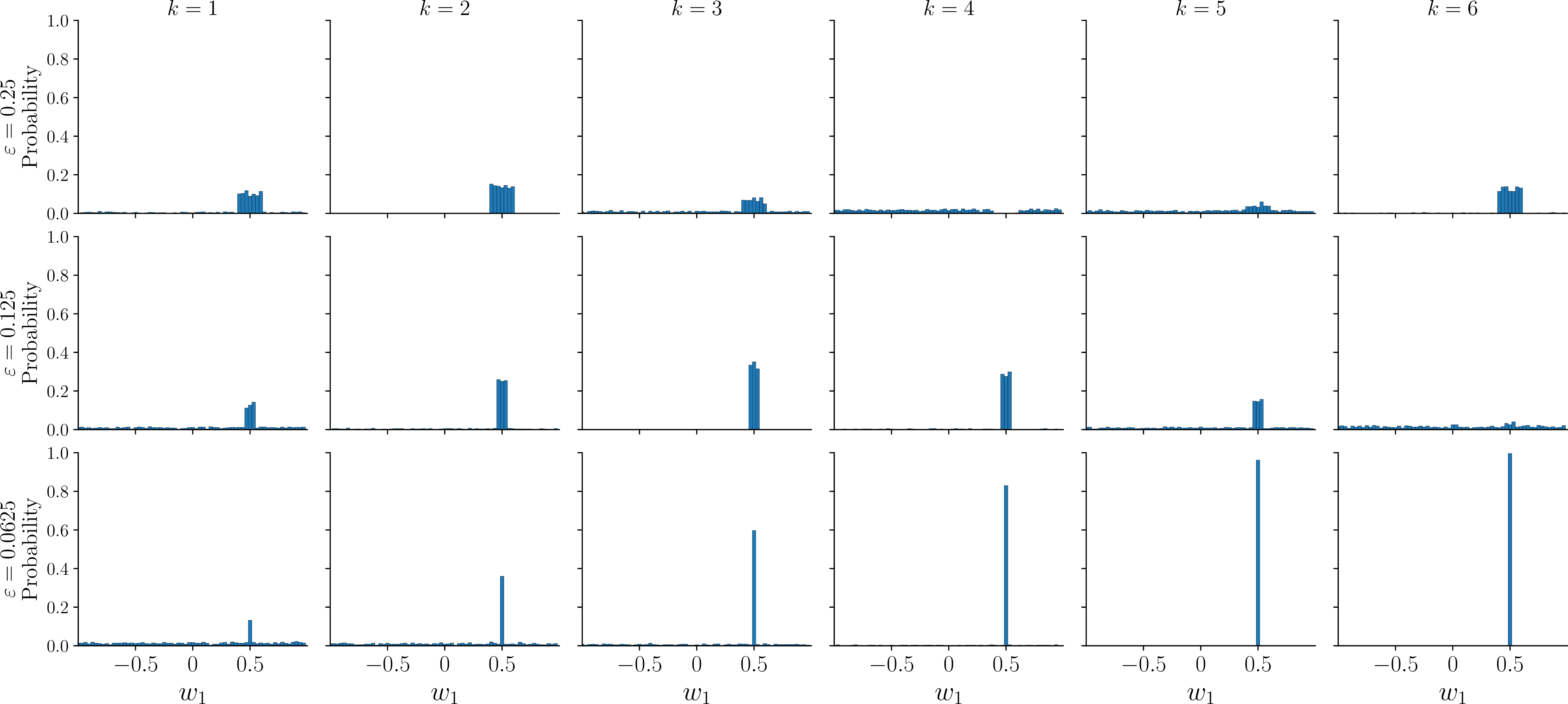
In Fig. 2, the number of marked solutions depends on the chosen oracle tolerance \(\varepsilon\). For \(\varepsilon = 2^{-1}, 2^{-2}, 2^{-3}\), we observe \(K_W=7,3,1\) marked candidates, respectively. Accordingly, the continuous theoretical optima for the number of Grover iterations (see Corollary 1) are \[k_{\mathrm{cont}}^\ast \approx 1.83,\quad 3.10,\quad 5.77,\] which correspond to the integer iteration counts \[k^\ast = 2,\quad 3,\quad 6,\] after rounding to the nearest integer, in agreement with the theoretical predictions. This dependence is reflected in the figure, where the probability mass concentrates more rapidly as the number of marked states increases.
7.1.0.2 Linear baseline problem (two-dimensional case):
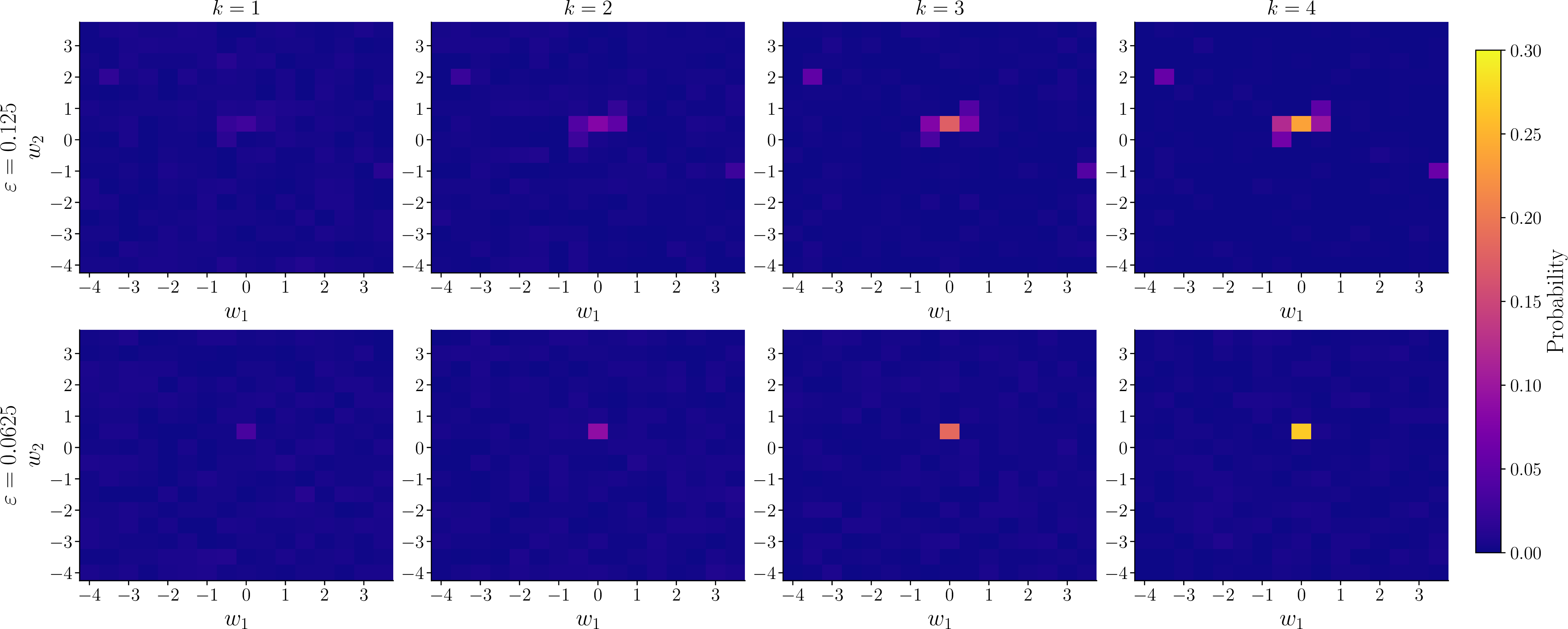
We extend the analysis to a two-dimensional parameter space using the ansatz \[u_2(x) = w_2\, x(1-x) + w_1\, x^2 (1-x)^2.\] In this setting, the parameter space is discretized uniformly with \(n_W = 8\) qubits, resulting in a search space of size \(N_W = 2^{n_W} = 256\).
As in the one-dimensional case, the oracle marks all parameter pairs \((w_1,w_2)\) whose residual falls below a prescribed tolerance \(\varepsilon\). For \(N=256\) and a single marked solution (\(K_W=1\)), the success probability after \(k\) Grover iterations is given by \[P(k) = \sin^2\!\big((2k+1)\theta\big), \qquad \theta = \arcsin\!\left(\frac{1}{16}\right).\] For \(k=4\), this yields a probability of approximately \(0.29\), which is shown by Fig. 3. In contrast to the one-dimensional case, the solution structure now appears as localized regions in a two-dimensional landscape, illustrating that the method naturally extends to higher-dimensional parameter spaces.
7.2 Experiment 2: Influence of Spatial Resolution↩︎
In this experiment, we isolate the residual-threshold oracle from the subsequent amplitude-amplification dynamics and study the influence of the spatial resolution. Unlike in Experiment 1, the oracle is evaluated directly for all \(w\in W_m\), without applying amplitude amplification.
We consider the linear boundary value problem \[\label{eq:experiment295problem} u''(x)+x=0, \qquad x\in[0,1], \qquad u(0)=u(1)=0,\tag{16}\] corresponding to Eq. 10 , with exact solution\(u^\ast(x)=\tfrac16 x(1-x^2)\). We compare the expressive ansatz \(u_3(x)=w_2x(1-x^2)\), which is exact for \(w_2^\ast=\tfrac16\), with the restricted ansatz \(u_1(x)=w_2x(1-x)\). For \(u_1\), \(r_C(x,w_2)=x-2w_2\), and minimizing the mean absolute residualover \([0,1]\) gives \(w_2^\ast=\tfrac14\).
We fix the parameter-space discretization to \(n_W=4\), the target-register precision to \(p_Z=5\), and choose \(n_Z\) according to the heuristic estimate in Eq. 15 . Only the spatial resolution \(n_X\) is varied.
7.2.1 Residual Measures↩︎
For a pointwise residual \(r(x_i,w)\), we define the aggregated collocation residual by \[\label{eq:aggregated95collocation95residual} \bar r(w) = \frac{1}{N_X} \sum_{i=0}^{N_X-1} |r(x_i,w)|.\tag{17}\] We distinguish the analytical reference residual \(\bar r_C\), obtained using the exact derivative of the ansatz; the finite-difference residual \(\bar r_{FD}\), obtained using \(D_h^2u\); and the quantum residual \(\bar r_Q\), evaluated by the reversible fixed-point arithmeticcircuit.
Since all three residuals are evaluated on the same spatial and parameter grids, the difference between \(\bar r_C\) and \(\bar r_{FD}\) captures effects of the discrete residual evaluation, whereas the difference between \(\bar r_{FD}\) and \(\bar r_Q\) isolates the additional fixed-point quantization error. We further use \[r_C^{\min}(w) = \min_i |r_C(x_i,w)|, \qquad r_C^{\max}(w) = \max_i |r_C(x_i,w)|\] to characterize the spatial variation of the analytical residual.
For both ansatz functions considered below, the centered finite-difference approximation of the second derivative is exact at interior grid points. The dependence on \(n_X\) therefore results from spatial sampling, aggregation over collocation points, boundary treatment, and fixed-point quantization rather than finite-difference truncation error.
7.2.2 Ansatz Function \(u_3\)↩︎
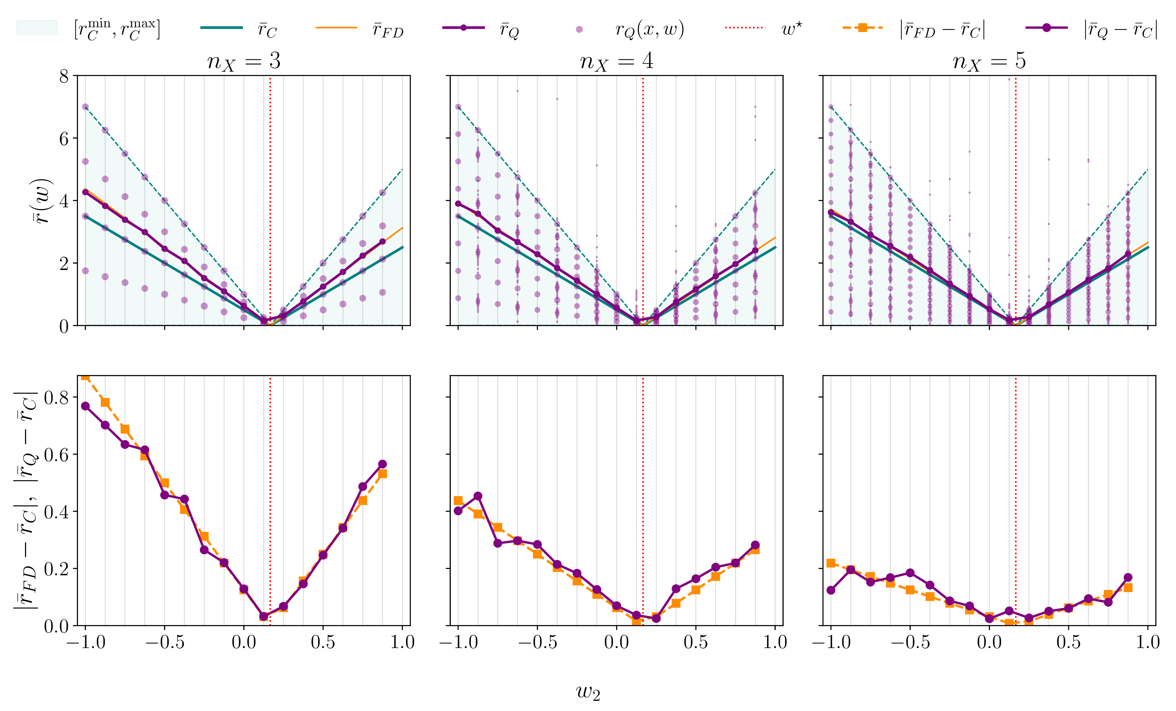
For \(u_3(x)=w_2x(1-x^2),\) the analytical residual is \(r_C(x,w_2)=(1-6w_2)x.\) Hence, the exact solution is contained in the ansatz space and is attained at \(w_2^\ast=\tfrac16\). Since this value is not represented exactly on the chosen parameter grid, the nearest admissible value is \(w_2=\tfrac18\).
Figure 4 shows that all three residual evaluations attain their minimum near this discretized optimum. The agreement between \(\bar r_{FD}\) and \(\bar r_C\) confirms the exactness of the centered finite difference for this cubic ansatz, while deviations of \(\bar r_Q\) from \(\bar r_{FD}\) quantify the remaining fixed-point effects.
7.2.3 Ansatz Function \(u_1\)↩︎
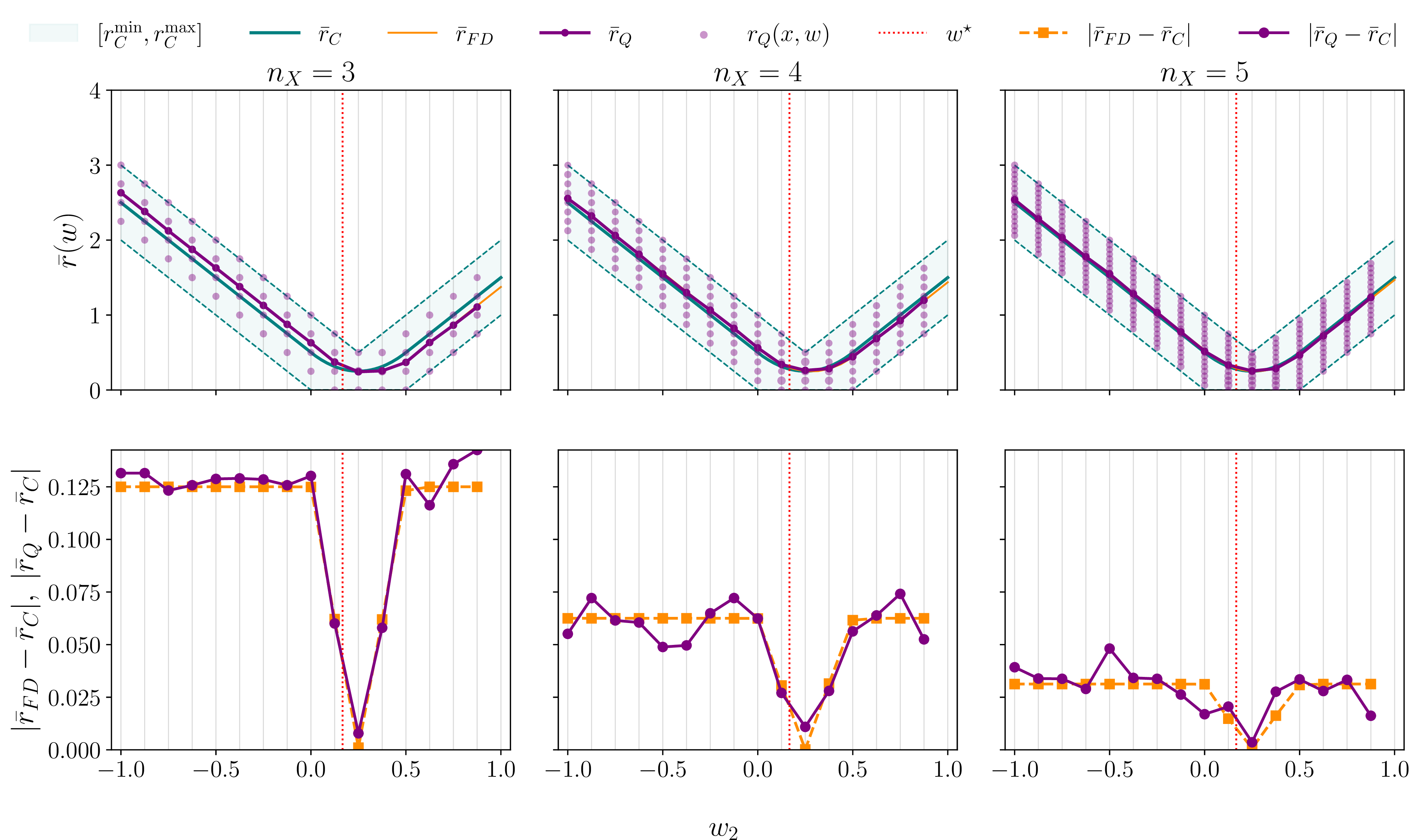
For \(u_1(x)=w_2x(1-x),\) the analytical residual is \(r_C(x,w_2)=x-2w_2.\) The exact solution is not contained in this ansatz space. Minimizing the mean absolute residual over \(x\in[0,1]\) gives \(w_2^\ast=\tfrac14\), rather than \(\tfrac16\), because \(2w_2\) must equal the median of the interval. The residual minimum therefore remains nonzero even at the optimal parameter value.
As shown in Fig. 5, the quantum residual closely follows the finite-difference residual, whereas the nonvanishingminimum is caused by the limited expressivity of the ansatz rather than by the reversible implementation.
7.2.4 Comparison of Residual-Evaluation Errors↩︎
To quantify deviations from the analytical reference, we use \[\label{eq:experiment295mape} \operatorname{MAPE}(\bar r,\bar r_C) = \frac{100\%}{N_W} \sum_{w\in W_m} \frac{|\bar r(w)-\bar r_C(w)|}{|\bar r_C(w)|}.\tag{18}\] For the chosen parameter grid, the denominator does not vanish for any evaluated parameter value.
Figure 6 compares the MAPE of \(\bar r_{FD}\) and \(\bar r_Q\) for both ansatz functions. The finite-difference error reflects the discrete collocation and boundary treatment, while the additional quantum error is caused by fixed-point quantization.
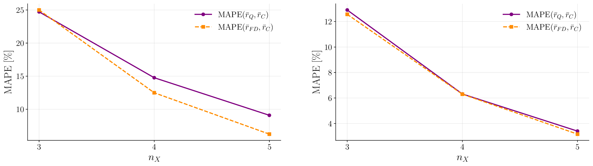
The results separate three effects: the parameter-grid error for\(u_3\), the intrinsic ansatz error for \(u_1\), and the fixed-point quantization error of the reversible residual evaluation. We next study how the resulting oracle phases affect the amplitude-amplification dynamics.
7.2.5 Empirical Verification of the Amplification Dynamics↩︎
According to Theorem 1, each spatial state \(x_i\) evolves with the effective Grover angle \[\theta_i = \arcsin\!\left( \sqrt{\frac{|\mathcal{M}_i|}{N_W}} \right), \qquad \mathcal{M}_i = \{j\in\mathcal{I}_W\mid \chi(i,j)=1\},\] where \(\mathcal{M}_i\) denotes the set of marked parameter indices at the collocation point \(x_i\). Larger marked sets therefore leadto faster amplification, whereas smaller sets produce slower but more selective dynamics.
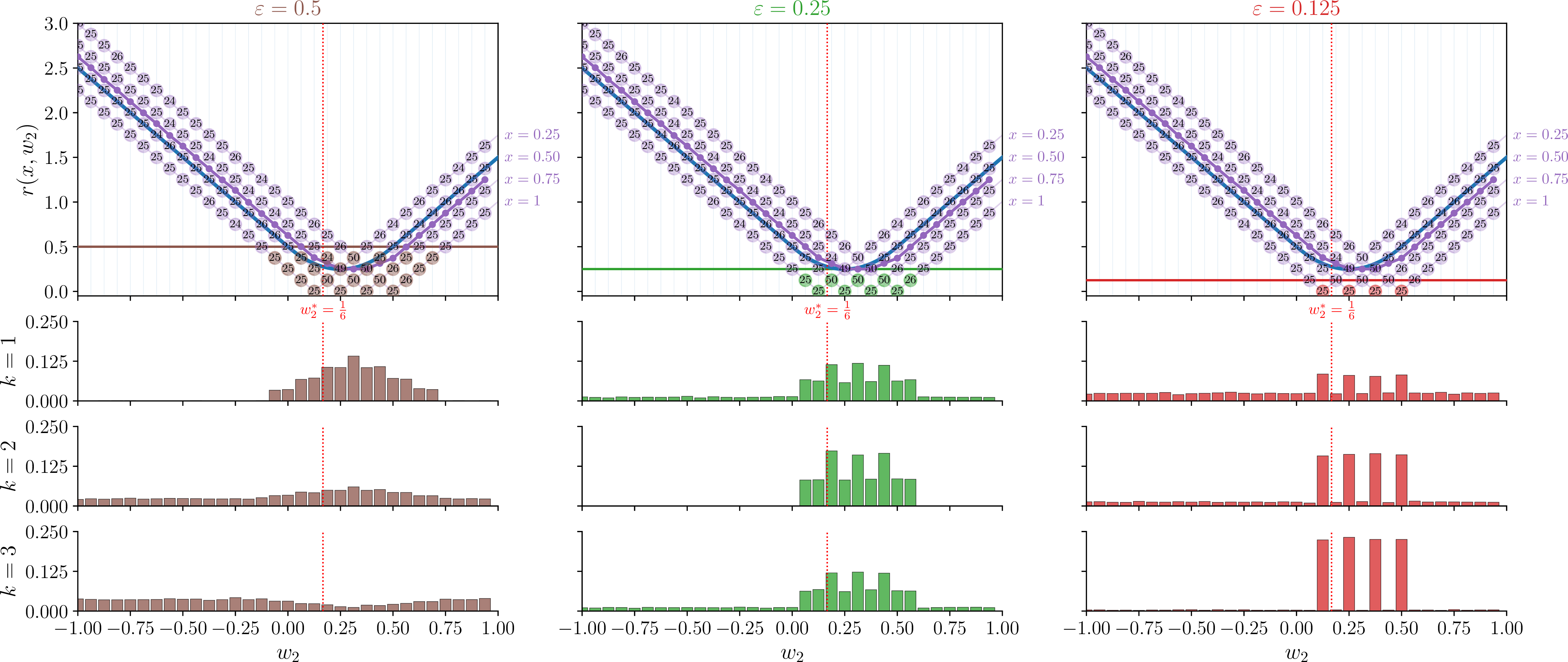
We consider \(n_X=3\), \(n_W=5\), and \(\varepsilon\in\{0.125,0.25,0.5\}\). For each \(w_j\in W_m\), the weighted-oracle response \(q(w_j)\) is the fraction of collocation points satisfying the residual threshold. Hence, \[\frac{1}{N_W} \sum_{j=0}^{N_W-1}q(w_j)\] gives the average oracle response over the parameter register.
For \(\varepsilon=0.5,0.25,0.125\), the marked-set sizes are \(|\mathcal{M}_i|=7,3,1\), respectively, for every spatial sector. Thus, all sectors have identical amplification angles, and the dynamics reduce to the standard Grover regime of Corollary 1. The corresponding continuous optimal iteration counts, \[k_{\mathrm{cont}}^\ast = \frac{\pi}{4\theta_i} -\frac{1}{2},\] are approximately \(1.1\), \(2.0\), and \(3.9\).
Figure 7 shows the residual functions, marked regions, and measured parameter distributions after \(k=1,2,3\) amplification iterations. Decreasing \(\varepsilon\)narrows the marked region and reduces the amplification angle. Larger tolerances therefore lead to faster amplification and earlier overrotation, whereas smaller tolerances yield slower but more selective concentration near \(w^\ast=\tfrac16\). The observed dynamics agree with Theorem 1.
7.3 Experiment 3: Nonlinear Residuals and Finite-Precision Effects↩︎
We consider the manufactured nonlinear boundary value problem \[u''(x) + u(x) + \alpha u(x)^2 + 2\lambda - \lambda x(1-x) - \alpha \lambda^2 x^2(1-x)^2 = 0,\] for \(x\in[0,1]\) with homogeneous boundary conditions \(u(0)=u(1)=0\) and nonlinearity parameters \(\alpha\in\{8,16,32\}.\) By construction, \(u^\ast(x) = \lambda x(1-x)\) is an exact solution. Throughout this experiment, we set \(\lambda=\frac{1}{3}.\)
In contrast to the preceding experiments, the residual now contains the nonlinear term \(u(x)^2\). The goal of this experiment is therefore twofold:
to analyze how increasing nonlinearity modifies the residual landscape and the resulting amplification behavior,
to quantify the influence of finite-precision arithmetic on the oracle evaluation.
7.3.1 Nonlinearity-Induced Residual Structure↩︎
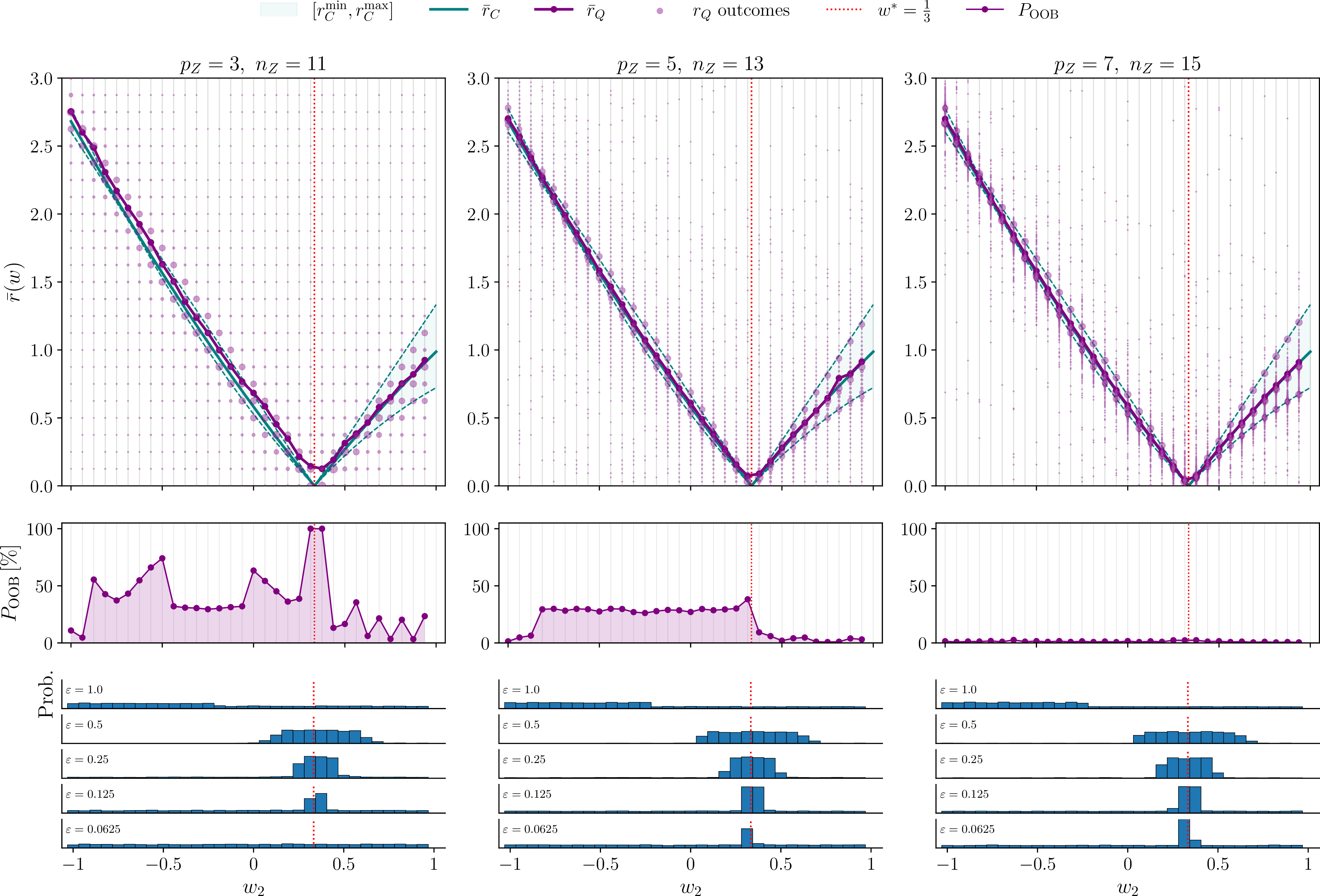
We first fix the value-register precision to \(p_Z=5\) and vary the nonlinearity parameter \(\alpha\). For weak nonlinearity, the residual landscape is sharply localized around the physical solution \(w^\ast=\frac{1}{3}\). As \(\alpha\) increases, additional low-residual regions and local minima emerge.
Although the problem is constructed so that \(u^\ast(x)=\lambda x(1-x)\) remains an exact solution, the nonlinear residual creates competing parameter regions with comparable residual values. Consequently, the oracle assigns significant response toseveral regions rather than marking a single isolated one.
This structure is reflected in the amplified sampling distributions in the lower panels of Fig. 8. Larger tolerances \(\varepsilon\) produce broader amplified regions, whereas smaller tolerances increase selectivity and suppress parts of the secondary minima. Even for strong nonlinearity, \(\alpha=32\), the amplification process reliably identifies the dominant low-residual regions.
This behavior agrees with the weighted-oracle framework of Theorem 1, in whichseveral parameter regions with large local oracle response \(q(w_j)\) are amplified simultaneously.
7.3.2 Finite-Precision Quantization Effects↩︎
We now fix the nonlinearity parameter to \(\alpha=8\) and investigate the influence of finite-precision arithmetic by varying the value-register precision \[p_Z\in\{3,4,5\}.\] As an empirical measure of quantization artifacts, we introduce the out-of-band probability \[P_{\mathrm{OOB}}(w) = 100 \sum_{o\in\mathcal{O}(w)} p(o\mid w)\, \mathbf{1}\!\left[ |r_Q(o,w)| \notin \left[ r_C^{\min}(w)-\delta_{\mathrm{band}}, r_C^{\max}(w)+\delta_{\mathrm{band}} \right] \right],\] which measures the fraction of quantum outcomes whose residual values lie outside the classical reference interval up to a small tolerance \(\delta_{\mathrm{band}}\). This tolerance prevents minor numerical deviations near the interval boundaries from being counted as meaningful discrepancies.
suppresses quantization-induced deviations in the
The results are shown in Fig. 8. Atlow precision, the quantum residual evaluation visibly deviates fromthe classical finite-difference reference because of rounding and limited residual resolution, as reflected by elevated values of \(P_{\mathrm{OOB}}\). Increasing the value-register precision systematically reduces these deviations and drives the quantum residual toward the classical discretized residual. Meanwhile, the dominant amplified parameter region remains stable, indicating that the amplification process is robust against moderate quantization errors. At very low precision, however, the residual grid may be too coarse for the prescribed oracle tolerance. For \(p_Z=3\) and \(\varepsilon=2^{-4}\), the residual spacing is \(2^{-3}\), so the threshold \(2^{-4}\) is not representable. Consequently, no parameter value satisfies the threshold condition and the oracle marks no admissible candidate. This failure is therefore caused not by quantization noise itself, but by insufficient fixed-point resolution. The oracle tolerance must remain compatible with the representable residual precision.
7.4 Experiment 4: Resource Scaling of the Oracle Implementation↩︎
After validating the oracle accuracy and amplification behavior,we analyze the resource requirements of the resulting quantum circuits. Since multi-controlled phase operations are not native to current gate-based quantum hardware, all circuits were transpiled into the native gate basis prior to resource estimation.
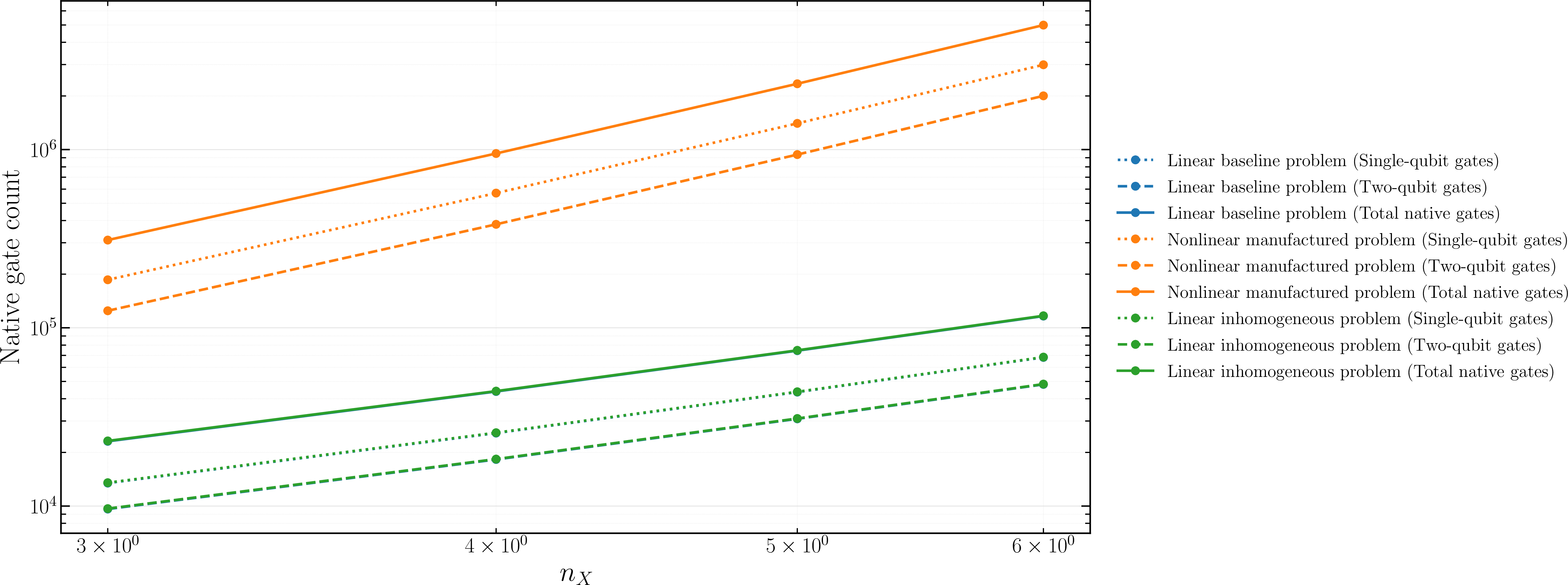
For the scaling analysis, we vary the spatial discretization parameter \(n_X\) while keeping \(p_W = 3\), \(p_Z = 3\), and the ansatz configuration fixed. For each transpiled circuit, we record the native single-qubit gate count, native two-qubit gate count, and total native gate count.
The observed scaling behavior is consistent with the theoreticaloracle-cost estimate derived in Theorem 3, \[C_{\mathrm{oracle}} = O\!\left( n_Z n_X^{D_f} n_W^{Q} (D_f+Q+1)^2 + n_Z^2 \right).\] which predicts polynomial growth with respect to the spatial discretization and parameter-space resolution.
Figure 9 shows the resulting scaling behavior for the benchmark problems considered in this work. Dotted lines denote native single-qubit gates, dashed lines native two-qubit gates, and solid lines the total native gate count after transpilation. Although the absolute gate counts differ between problem classes, all cases exhibit clear polynomial growth as \(n_X\) increases.
8 Conclusion↩︎
We have introduced a residual-based quantum collocation framework for one-dimensional boundary value problems and shown that its amplification dynamics differ fundamentally from the standard Grover setting. Rather than being governed by a single global marking condition, the search process evolves through a coherentsuperposition of spatially conditioned amplitude amplification rotations, with success probabilities determined by the distribution of local residual-threshold responses across the collocation grid.
The numerical experiments support the theoretical predictions and illustrate how discretization, ansatz expressivity, oracle tolerance, and finite-precision arithmetic influence both approximation quality and amplification behavior. Furthermore, the results show that the reversible residual oracle scales polynomially in the logarithmic size of the spatial register, while the parameter search benefits from the usual quadratic speedup provided by amplitude amplification. The present study focuses on low-dimensional polynomial ansatz spaces chosen to permit compact oracle constructions and modest qubit requirements, while the general framework is not restricted to these particular choices.Several directions for future research remain open. These include extensions to higher-dimensional partial differential equations, the investigation of more expressive ansatz spaces, adaptive collocation strategies, and scalability studies of the reversible oracle construction. Of particular interest are high-dimensional nonlinear PDEs arising in optimal control and stochastic control, such as Hamilton–Jacobi–Bellman equations,where classical discretization-based methods are often limited by the curse of dimensionality. Equally important is the study of the proposed framework on quantum hardware, where noise, decoherence and finite sampling effects may significantly influence the residual-based amplification dynamics. Overall, the framework establishes a foundation for residual-based quantum search methods for differential equations and highlights a novelconnection between collocation techniques and coherent amplitudeamplification.
9 Quantum Registers and Discretized Spaces↩︎
9.0.0.1 State register
Let \(X\) be an \(n_X\)-qubit register with associated Hilbert space \(\mathcal{H}_X := (\mathbb{C}^2)^{\otimes n_X}\) with \(N_X =2^{n_X}\). Its computational basis is \[\{\ket{i}_X\}_{i=0}^{N_X-1}, \qquad \langle i\mid j\rangle_X=\delta_{ij},\] where, for the binary expansion \[i=\sum_{j=0}^{n_X-1} b_j2^j, \qquad b_j\in\{0,1\},\] we define \[\ket{i}_X := \ket{b_{n_X-1}}\otimes\cdots\otimes\ket{b_0}.\] The register uses a fixed-point representation with \(f_X\) fractional bits. Thus, the same bitstring encodes the numerical value \[x=\sum_{j=0}^{n_X-1} b_j\,2^{j-f_X}, \qquad \ket{x}_X := \ket{b_{n_X-1}}\otimes\cdots\otimes\ket{b_0}.\] We write \(\ket{i}_X\) when treating computational basis states as indexed elements of \(\mathcal{H}_X\), and \(\ket{x}_X\) when interpreting them as encoded numerical values.
The spatial grid is a subset \[X\subset [0,1]\cap 2^{-f_X}\mathbb{N}_0.\] Not every computational basis state need correspond to an element of \(X\). In particular, the register may encode values slightly outside the physical domain \([0,1]\), as required for the reversible evaluation of finite-difference expressions such as \(x\pm h\).
A pure state of the register is a normalized vector \[\ket{\psi}_X = \sum_{i=0}^{N_X-1}\alpha_i\ket{i}_X, \qquad \alpha_i\in\mathbb{C}, \qquad \sum_{i=0}^{N_X-1}|\alpha_i|^2=1.\]
9.0.0.2 Parameter register
Let \[W_m \subset (2^{-f_w}\mathbb{Z})^m\] denote the set of all parameter vectors representable with the chosen fixed-point encoding for an \(m\)-parameter ansatz. A parameter vector \(w=(w_1,\dots,w_m)\in W_m\) consists of \(m\) components, each encoded as a signed fixed-point number with \(I_w\) integer bits and \(f_w\) fractional bits. Including the sign bit, each component requires \(n_w = 1 + I_w + f_w\) qubits.
If \(b^\ell_{n_w-1}\dots b^\ell_0\) denotes the bitstring encoding the component \(w_\ell\), then \[w_\ell = -\,b^\ell_{n_w-1}2^{\,n_w-1-f_w} + \sum_{s=0}^{n_w-2} b^\ell_s\,2^{\,s-f_w}, \qquad b^\ell_s\in\{0,1\}.\] which corresponds to the standard two’s-complement fixed-point representation.
The parameter register therefore consists of \(m\) blocks of \(n_w\) qubits and contains \(n_W = m n_w\) qubits in total.
Its Hilbert space is \(\mathcal{H}_W := (\mathbb{C}^2)^{\otimes n_W}\) with computational basis \[\{\ket{j}_W\}_{j=0}^{N_W-1}, \qquad N_W = 2^{n_W}.\] Each basis state \(\ket{j}_W\) encodes a parameter vector \[w_j = (w_{j,1},\dots,w_{j,m}) \in W_m,\] where each component \(w_{j,\ell}\) is obtained by decoding the corresponding block of \(n_w\) qubits.
9.0.0.3 Value register
Let the value register consist of \(n_Z\) qubits with \(f_Z\) fractional bits. For \(k\in\{0,\ldots,N_Z-1\}\), let \[k=\sum_{j=0}^{n_Z-1} b_j2^j, \qquad b_j\in\{0,1\},\] be the binary representation associated with the computational basis state \(\ket{k}_Z\). The corresponding signed fixed-point value is \[z_k = - b_{n_Z-1} 2^{\,n_Z-1-f_Z} + \sum_{j=0}^{n_Z-2} b_j\,2^{\,j-f_Z}.\] The Hilbert space of the value register is \(\mathcal{H}_Z := (\mathbb{C}^2)^{\otimes n_Z}\) with computational basis \[\{\ket{k}_Z\}_{k=0}^{N_Z-1}, \qquad N_Z = 2^{n_Z}.\] We denote by \[\begin{align} \label{def95value95register} Z=\{z_k\}_{k=0}^{N_Z-1}\subset 2^{-f_Z}\mathbb{Z} \end{align}\tag{19}\] the set of all values representable by this fixed-point encoding.
10 QFT-based arithmetic↩︎
We use standard QFT-based reversible arithmetic primitives for modular addition and multiplication; see, e.g., [27]–[29]. For the residual oracle, we need only the resulting scaling for polynomial terms. We therefore record the following estimate for monomials of the form \(x^{k_x}w^{k_y}\).
Let \(X\), \(W\), and \(Z\) be computational registers of sizes \(n_X\), \(n_W\), and \(n_Z\), respectively, and let \(N_Z=2^{n_Z}\). We consider the reversible modular map \[\label{eq:poly95map} \ket{x}_X\ket{w}_W\ket{z}_Z \longmapsto \ket{x}_X\ket{w}_W \ket{z\oplus x^{k_x}w^{k_y}}_Z ,\tag{20}\] where the addition is modulo \(N_Z\). Throughout this estimate, arithmetic is understood at the level of the encoded integers; fixed-point scaling factors only change the rotation angles and not the asymptotic gate count.
Applying the QFT to the target register \(Z\) turns the modular addition in 20 into multiplication by the phase \[\exp\!\left(2\pi i\,\frac{x^{k_x}w^{k_y}q}{N_Z}\right),\] where \(q\) denotes the Fourier-basis index of the \(Z\)-register. Expanding \(x\), \(w\), and \(q\) in binary expresses this phase as a product of multi-controlled phase rotations. Each contribution is controlled on at most \(k_x\) bits from the \(X\)-register, \(k_y\) bits from the \(W\)-register, and one Fourier bit of the \(Z\)-register. Repeated bit indices only merge or reduce controls and therefore do not affect the upper bound below.
Lemma 2 (Gate complexity of QFT-based polynomial arithmetic). Let \(U_{\mathrm{poly}}\) denote the QFT-based reversible implementation of a monomial contribution \[c\,x^{k_x}w^{k_y}\] to the modular addition in 20 , where \(x\) and \(w\) are scalar variables encoded in \(n_X\) and \(n_W\) qubits, respectively. Counting arbitrary one-qubit gates and CNOT gates as elementary, as in Barenco et al. [30], one has \[C(U_{\mathrm{poly}}) = O\!\left( n_Z n_X^{k_x}n_W^{k_y}(k_x+k_y+1)^2+n_Z^2 \right).\]
Proof. Write \[x=\sum_{i=0}^{n_X-1}2^i x_i, \qquad w=\sum_{j=0}^{n_W-1}2^j w_j, \qquad x_i,w_j\in\{0,1\}.\] Then \[x^{k_x} = \sum_{i_1=0}^{n_X-1}\cdots \sum_{i_{k_x}=0}^{n_X-1} 2^{i_1+\cdots+i_{k_x}} x_{i_1}\cdots x_{i_{k_x}},\] and analogously for \(w^{k_y}\). Hence, \(x^{k_x}w^{k_y}\) is a sum of at most \(n_X^{k_x}n_W^{k_y}\) bit monomials. Since repeated indices maybe removed using \(x_i^r=x_i\) and \(w_j^r=w_j\), each monomial depends on at most \(k_x+k_y\) distinct input bits.
In the Fourier basis, each bit monomial induces at most one phase rotation on each of the \(n_Z\) target qubits. Thus, at most \[n_Z n_X^{k_x}n_W^{k_y}\] multi-controlled one-qubit phase gates are required. Each has atmost \(c=k_x+k_y\) controls. By Corollary 7.6 of Barenco et al. [30], such a gate can be decomposed into \[O\!\left((c+1)^2\right) = O\!\left((k_x+k_y+1)^2\right)\] elementary one-qubit and CNOT gates. The phase accumulation therefore has complexity \[O\!\left( n_Z n_X^{k_x}n_W^{k_y}(k_x+k_y+1)^2 \right).\] Adding the \(O(n_Z^2)\) cost of the QFT and inverse QFT gives the stated bound. ◻
For signed fixed-point encodings, the sign bits only change the signs of the corresponding phase angles. The control structure, and hencethe asymptotic gate count in Lemma 2, remains unchanged.
11 Reversible Implementations↩︎
This appendix gives explicit reversible constructions of the residual, absolute-value, and threshold-subtraction operators \(U_r\), \(U_a\), and \(U_s\) entering \[U_c = (I_X\otimes I_W\otimes U_s\otimes I_A) (I_X\otimes I_W\otimes U_a) (U_r\otimes I_A).\] The register encodings are specified in Appendix 9.
Reversible Absolute-Value Operator↩︎
The \(n_Z\)-qubit value register uses two’s-complement fixed-point encoding with \(f_Z\) fractional bits. Its representable set \(Z\) is defined in 19 , with extremal values \[z_{\min}=-2^{\,n_Z-1-f_Z}, \qquad z_{\max}=2^{\,n_Z-1-f_Z}-2^{-f_Z}.\] Because \(|z_{\min}|\notin Z\), the reversible absolute-value operation uses two ancilla qubits, \[A=A_{\mathrm{sign}}\otimes A_{\mathrm{ind}},\] which store the input sign and indicate the exceptional value \(z_{\min}\), respectively.
The unitary \[U_a:\mathcal{H}_Z\otimes\mathcal{H}_A \longrightarrow \mathcal{H}_Z\otimes\mathcal{H}_A\] acts on clean ancillas as \[U_a\!\left( \ket{z}_Z\ket{0}_{A_{\mathrm{sign}}}\ket{0}_{A_{\mathrm{ind}}} \right) = \ket{\widetilde{|z|}}_Z \ket{\sigma(z)}_{A_{\mathrm{sign}}} \ket{\eta(z)}_{A_{\mathrm{ind}}},\] where \[\sigma(z)= \begin{cases} 0, & z\geq 0, \\ 1, & z<0, \end{cases} \qquad \eta(z)= \begin{cases} 1, & z=z_{\min}, \\ 0, & z\neq z_{\min},\end{cases}\] and \[\widetilde{|z|} = \begin{cases} |z|, & z\neq z_{\min}, \\ z_{\max}, & z=z_{\min}.\end{cases}\] This action is extended bijectively to the remaining computational basis states.
A reversible circuit first copies the sign into \(A_{\mathrm{sign}}\), detects \(z_{\min}\) in \(A_{\mathrm{ind}}\), and then, for non-exceptional negative inputs, conditionally applies bitwise inversion followed by an increment, for example with a QFT-based adder. For \(z=z_{\min}\), the output \(z_{\max}\) together with \(A_{\mathrm{ind}}=1\) preserves reversibility. Since \(z_{\min}\) is thereby mapped to a large positive value, it remains outside the admissible tolerance region \[|z|<\varepsilon_{\mathrm{tol}}\] and cannot be misclassified as a valid solution.
Reversible Subtraction of the Tolerance Threshold↩︎
Let \(N_Z=2^{n_Z}\), and let \[k'=\sum_{s=0}^{n_Z-1}k'_s2^s, \qquad k'_s\in\{0,1\},\] be the integer encoding of \(-\varepsilon_{\mathrm{tol}}\). Threshold subtraction is the modular constant addition \[U_s:\mathcal{H}_Z\longrightarrow\mathcal{H}_Z, \qquad U_s\ket{k}_Z=\ket{k\oplus k'}_Z, \qquad k\oplus k':=(k+k')\bmod N_Z.\] On the admissible computational subspace used by the oracle, theregister range is chosen so that this modular operation coincides with ordinary subtraction and no wrap-around occurs.
Using Draper addition, \[U_s = \mathrm{QFT}_{n_Z}^{-1}U_\phi\mathrm{QFT}_{n_Z}.\] For the \(r\)-th value qubit, define \[\Pi^{(0)}_{Z_r} = \ket{0}\bra{0}_{Z_r}\otimes I_{\mathrm{rest}}, \qquad \Pi^{(1)}_{Z_r} = \ket{1}\bra{1}_{Z_r}\otimes I_{\mathrm{rest}}.\] The bit \(k'_s\) contributes the phase \(2\pi k'_s2^{\,s+r-n_Z}\) to qubit \(Z_r\), so that \[U_\phi = \prod_{r=0}^{n_Z-1} \left( \Pi^{(0)}_{Z_r} + \exp\!\left[ 2\pi i\sum_{s=0}^{n_Z-1}k'_s2^{\,s+r-n_Z} \right] \Pi^{(1)}_{Z_r} \right).\] Thus, \(U_\phi\) has the same phase-accumulation structure as register-based QFT addition, except that the controls \(k'_s\) are classical bits of a fixed constant. More general out-of-place and register-based constructions are described in [27]–[29].
Reversible Residual Operator↩︎
The residual operator acts on \(\mathcal{H}_X\otimes\mathcal{H}_W\otimes\mathcal{H}_Z\). The spatial register encodes grid points \(x_i\in X\) with spacing \(h=2^{-f_X}\) and has sufficient overflow capacity to represent\(x_i\pm h\).
For \[r(x,w)=D_h^2u(x,w)+f\bigl(x,u(x,w)\bigr),\] let \(\rho(i,j)\) be the unique index satisfying \[\label{definition95discretized95residual} z_{\rho(i,j)} = r(x_i,w_j) = D_h^2u(x_i,w_j)+f\bigl(x_i,u(x_i,w_j)\bigr).\tag{21}\] The unitary \(U_r=U_fU_{D^2}\) accumulates the encoded residual modulo \(N_Z\): \[U_r\ket{i}_X\ket{j}_W\ket{k}_Z = \ket{i}_X\ket{j}_W\ket{k\oplus\rho(i,j)}_Z,\] where \(\oplus\) denotes addition modulo \(N_Z\). Hence, \[U_r\ket{i}_X\ket{j}_W\ket{0}_Z = \ket{i}_X\ket{j}_W\ket{\rho(i,j)}_Z.\] The centered finite-difference approximation is \[D_h^2u(x_i,w_j) = \frac{u(x_i-h,w_j)-2u(x_i,w_j)+u(x_i+h,w_j)}{h^2}.\] Reversible translations of the spatial register provide coherentaccess to \(x_i-h\), \(x_i\), and \(x_i+h\), after which inverse translations restore the original spatial encoding. The three contributions are accumulated coherently in the value register.
The ansatz is linear in \(w=(w^0,\ldots,w^{m-1})\) and polynomial in \(x\), \[u(x,w) = \sum_{\ell=0}^{m-1}w^\ell\phi_\ell(x), \qquad \phi_\ell(x) = \sum_{d=0}^{D_\ell}a_{\ell,d}x^d.\] Consequently, the finite-difference contribution consists of terms of the form \(c\,w^\ell x_i^d\), with fixed coefficients \(c\).
The forcing term is assumed to be polynomial in its second argument, \[\label{def:forcing95term} f(x,u)=\sum_{q=0}^{Q}b_q(x)u^q,\tag{22}\] where each \(b_q(x)\) is polynomial in \(x\). Substitution of the ansatz therefore yields a polynomial in \(x\) and \(w\), including monomials \(w^{j_1}\cdots w^{j_q}\).
Let \(\delta(i,j)\) and \(\eta(i,j)\) encode \(D_h^2u(x_i,w_j)\) and \(f(x_i,u(x_i,w_j))\), respectively. Then \[U_{D^2}\ket{i}_X\ket{j}_W\ket{k}_Z = \ket{i}_X\ket{j}_W\ket{k\oplus\delta(i,j)}_Z,\] and \[U_f\ket{i}_X\ket{j}_W\ket{k}_Z = \ket{i}_X\ket{j}_W\ket{k\oplus\eta(i,j)}_Z.\] Thus, \[\rho(i,j)=\delta(i,j)\oplus\eta(i,j),\] and the composition \(U_r=U_fU_{D^2}\) has the stated action. Since both subroutines are reversible, the induced computational-basismap is bijective and therefore unitary.