Calibration, Not Compilation: Detecting and Repairing
Misspecified Probabilistic Programs Written by Language Models
June 30, 2026
1 Introduction↩︎
Probabilistic programming languages (PPLs) such as Stan [1], Pyro/NumPyro [2], [3], and PyMC let practitioners specify a generative model and obtain a posterior by general-purpose inference. Writing a correct probabilistic program, however, requires statistical expertise: one must choose an appropriate likelihood, give parameters valid support, capture the dispersion and tail behavior of the data, and pick a parameterization that the sampler can actually explore. Large language models are increasingly used to draft such programs, and a tempting deployment pattern is to wrap the LLM in an agentic loop that “tests” its output and iterates.
The difficulty is that the usual notion of a test does not apply. A probabilistic program is not correct because it runs; it is correct because its posterior is well-calibrated and its predictions match held-out data. A model that uses a Gaussian likelihood for heavy-tailed data, a Poisson likelihood for over-dispersed counts, or a centered parameterization for a hierarchical funnel will compile, run under NUTS, return finite samples, and pass every conventional unit test—while being statistically wrong in a way that no amount of code inspection on a neutral task description can reveal. We call such errors code-invisible misspecification.
Our central claim is that the right verifier for LLM-written probabilistic programs is the Bayesian workflow [4]: simulation-based calibration (SBC) [5], posterior predictive checks (PPC) [6], sampler diagnostics such as \(\hat{R}\) [7] and divergent transitions [8], and held-out predictive density. These quantities form a calibration oracle that, unlike a test suite, is sensitive precisely to statistical error. We study it as both a detector (does it flag misspecification a test misses?) and a repair signal (does feeding it back to the writer fix the program?), on a controlled benchmark and on programs models write from scratch. In one phrase: for probabilistic programs, correctness is calibration, not compilation.
We make three contributions.
A misspecification benchmark and the detection result. We build a benchmark of \(14\) misspecification types across \(10\) model families (\(200\) instances), all of which compile and run. The calibration oracle flags the bug in \(88\%\) of cases (\(93\%\) of code-invisible ones) at a \(2\%\) false-positive rate (detection AUC \(0.97\)), versus \(0\%\) for a unit-test oracle. Each error type lights up the right diagnostic, and the oracle further localizes the bug type with \(75\%\) top-2 accuracy.
It does not need a correct program. A reference-free oracle (PPC + sampler + SBC) detects \(62\%\) of bugs; adding a classical GLM baseline reaches \(68\%\), and an automated model search (LOO over a small standard library) reaches \(78\%\)—all without a hand-written correct program. The \(88\%\) “reference” figure is an upper bound that assumes the correct program is known. An ablation shows held-out density is the strongest single component, while SBC alone cannot detect model–data misspecification.
Calibration-as-oracle repair. Used as feedback in an LLM repair loop and compared against no feedback (self-refine) and unit-test feedback, calibration is the strongest signal at every capability level able to use it, lifting GPT-5.1 from \(33\%\!\to\!92\%\) and Claude Sonnet 4.6 from \(75\%\!\to\!100\%\) on code-invisible bugs across fifteen models.
Two robust phenomena. (a) Unit-test feedback is harmful: “all checks pass” suppresses repair, so test feedback is \(\le\) no feedback (Claude: \(25\%\) vs.\(75\%\)). (b) The benefit of calibration feedback is non-monotone in capability—negligible for models too weak to act on a diagnostic or strong enough to repair blindly, and largest for strong-but-unsaturated models (GPT-5.1, Claude).
Real, not just injected, failures. On programs LLMs write from scratch for neutral briefs, \(15\)–\(47\%\) of runnable ones are statistically misspecified (unit tests flag none), and calibration repair significantly beats LLM-as-judge review, a Bayesian checklist, and data-summary self-debug (\(p<0.05\), paired McNemar).
2 Related Work↩︎
2.0.0.1 Bayesian workflow and model criticism.
Posterior predictive checks [6], simulation-based calibration [5], improved \(\hat{R}\) and tail diagnostics [7], and divergence-based geometry diagnostics for HMC/NUTS [8], [9] are the standard tools for criticizing a fitted Bayesian model, codified as the Bayesian workflow [4]. We repurpose these tools as an automated oracle and repair signal rather than a human-facing diagnostic dashboard.
2.0.0.2 LLMs for probabilistic and statistical modeling.
Recent work uses LLMs to elicit priors [10], to quantify uncertainty of LLM-based systems by treating prompts as Bayesian parameters [11], and to draft or discover probabilistic models. These efforts largely assume the generated model is structurally acceptable; we instead target the detection and repair of statistical misspecification using calibration as the criterion.
2.0.0.3 LLM code repair and self-improvement.
Iterative self-correction [12] and test-driven program repair use execution traces or failing unit tests as the feedback signal. For ordinary software this is appropriate; for probabilistic programs the analogous “it runs and returns numbers” signal is exactly the false all-clear we show to be harmful. Our contribution is to replace the test oracle with a calibration oracle.
3 Method↩︎
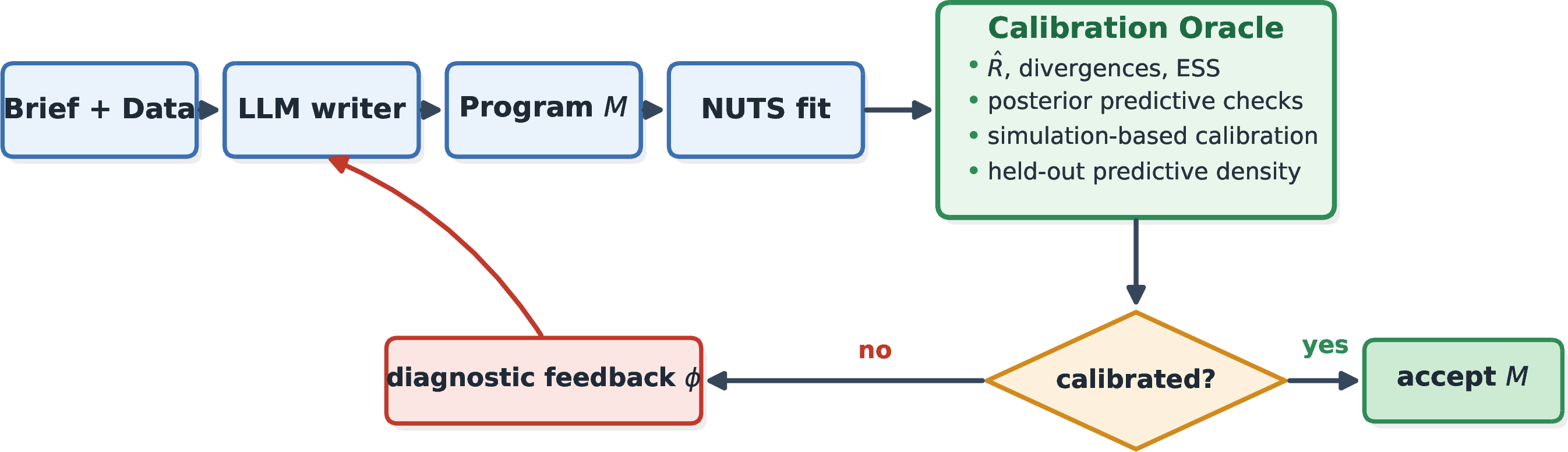
Figure 1 summarizes our approach: an LLM drafts a probabilistic program, a sampler fits it, a calibration oracle criticizes the fit, and—if the fit is not calibrated—a structured diagnostic is fed back for repair. We now formalize each component.
3.1 Problem Formalization↩︎
A task is a tuple \((\,b,\,\mathcal{D}_{\mathrm{tr}},\,\mathcal{D}_{\mathrm{te}})\) with a natural-language brief \(b\) and data drawn from an unknown generating process \(y\sim p^\star\). A candidate program \(M\) defines a joint density \(p_M(y,\theta)=p_M(\theta)\,p_M(y\mid\theta)\) over parameters \(\theta\) and observations \(y\); fitting yields a posterior \(\hat{\pi}(\theta)\approx p_M(\theta\mid \mathcal{D}_{\mathrm{tr}})\) and a posterior predictive
\(p_M(\tilde{y}\mid \mathcal{D}_{\mathrm{tr}})=\int p_M(\tilde{y}\mid\theta)\,\hat{\pi}(\theta)\,d\theta\). We call \(M\) statistically correct if its predictive distribution is
indistinguishable from \(p^\star\) under a chosen family of discrepancies, and misspecified otherwise. Importantly, two programs can induce very different \(p_M\) while being
syntactically interchangeable: e.g.Poisson vs.NegativeBinomial differ in one token but encode different dispersion.
3.2 The Calibration Oracle↩︎
The oracle \(O(M,\mathcal{D})\) aggregates four families of Bayesian-workflow diagnostics.
3.2.0.1 Posterior predictive checks.
For a test statistic \(T\), the two-sided posterior-predictive tail probability is \[p_T \;=\; \min\!\big(u,\,1-u\big),\quad u=\Pr_{\tilde{y}\sim p_M(\cdot\mid\mathcal{D}_{\mathrm{tr}})}\!\big[T(\tilde{y})\ge T(y_{\mathrm{obs}})\big], \label{eq:ppc}\tag{1}\] estimated from posterior-predictive replicates over \(T\in\{\mathrm{mean},\mathrm{sd},\mathrm{max},\#\text{zeros}\}\). Under correct specification \(u\) is approximately uniform, so \(p_T\) concentrates near \(\tfrac12\); a value near \(0\) indicates the model cannot reproduce that aspect of the data.
3.2.0.2 Simulation-based calibration.
For a scalar \(g(\theta)\), draw \(\theta_0\sim p_M(\theta)\), \(y\sim p_M(\cdot\mid\theta_0)\), fit, and form the rank of the prior draw among \(S\) posterior draws, \[r=\sum_{s=1}^{S}\mathbf{1}\!\left[g(\theta_s)<g(\theta_0)\right],\qquad r\sim\mathrm{Uniform}\{0,1,\dots,S\} \label{eq:sbc}\tag{2}\] where the uniformity holds exactly when inference is exact and the model is well-specified [5]; systematic deviation of the rank histogram flags inference or specification error.
3.2.0.3 Sampler geometry.
The split-\(\hat{R}\) [7], minimum bulk ESS, and the number of divergent transitions of NUTS [8], [9] detect parameterizations whose posterior geometry the sampler cannot traverse (e.g.the hierarchical funnel).
3.2.0.4 Held-out predictive density.
The pointwise log predictive density \[\mathrm{lppd}(M)=\frac{1}{|\mathcal{D}_{\mathrm{te}}|}\sum_{i\in\mathcal{D}_{\mathrm{te}}}\log \frac{1}{S}\sum_{s=1}^{S} p_M(y_i\mid\theta_s) \label{eq:lppd}\tag{3}\] is a Monte-Carlo estimate of the log score, a strictly proper scoring rule [13]. By Gibbs’ inequality, \[\mathbb{E}_{y\sim p^\star}\!\big[\log p_M(y)\big]\;\le\;\mathbb{E}_{y\sim p^\star}\!\big[\log p^\star(y)\big], \label{eq:gibbs}\tag{4}\] with equality iff \(p_M=p^\star\); hence a misspecified \(M\) has strictly lower expected lppd than the reference and the ranking is consistent as \(|\mathcal{D}_{\mathrm{te}}|\to\infty\).
3.2.0.5 Verdict.
Writing \(\mathbf{1}[\cdot]\) for the indicator, the calibration oracle returns \[\begin{align} O(M,\mathcal{D})=\;&\mathbf{1}[\text{ran}]\,\wedge\,\mathbf{1}[\hat{R}<1.05]\,\wedge\,\mathbf{1}[\#\mathrm{div}\le 15]\\ &\wedge\,\mathbf{1}[\textstyle\min_T p_T\ge\alpha]\,\wedge\,\mathbf{1}[\mathrm{lppd}\ge\mathrm{lppd}^\star-\delta], \end{align} \label{eq:verdict}\tag{5}\] with \(\alpha=0.01\), \(\delta=0.15\) nats, and \(\mathrm{lppd}^\star\) the reference. The competing unit-test oracle \(O_{\mathrm{u}}\) returns “pass” iff the program compiles, runs, and yields finite samples of the right shape.
3.3 Why Tests Fail and Calibration Succeeds↩︎
The two statements below are elementary—they formalize intuition rather than contribute new theory; our contribution is the framing, benchmark, and empirical study, not the propositions themselves.
Proposition 1 (Blindness of the test oracle). \(O_{\mathrm{u}}(M,\mathcal{D})\) is a function only of the program’s executability and output type, not of \(p_M\) or \(p^\star\). Hence for any two executable programs \(M_1,M_2\) returning finite samples of the same shape, \(O_{\mathrm{u}}(M_1)=O_{\mathrm{u}}(M_2)\) regardless of whether either is misspecified. On a family of misspecifications that all execute (our code-invisible* class), \(O_{\mathrm{u}}\) is therefore uninformative: its detection rate equals its base “pass” rate, independent of correctness.*
This is immediate from the definition of \(O_{\mathrm u}\), but it is the crux: a passing test conveys zero information about statistical correctness for code-invisible bugs.
Proposition 2 (Detection by calibration). Let \(M\) be misspecified in a statistic \(T\), i.e.\(T(y_{\mathrm{obs}})\) lies in the tails of \(p_M(T(\tilde{y})\mid \mathcal{D}_{\mathrm{tr}})\). Then as the number of posterior-predictive replicates grows, the estimated \(p_T\to \min(u,1-u)\) with \(u\to 0\) or \(1\), so \(O\) flags \(M\) at any fixed threshold \(\alpha>0\). Analogously, a parameterization with unreachable geometry yields \(\hat{R}>1\) and divergences bounded away from \(0\), and a misspecified likelihood yields strictly lower expected lppd than the reference. Thus \(O\) is a consistent detector for misspecification expressed through its diagnostics.
3.4 Bug Taxonomy: Visible vs.Invisible↩︎
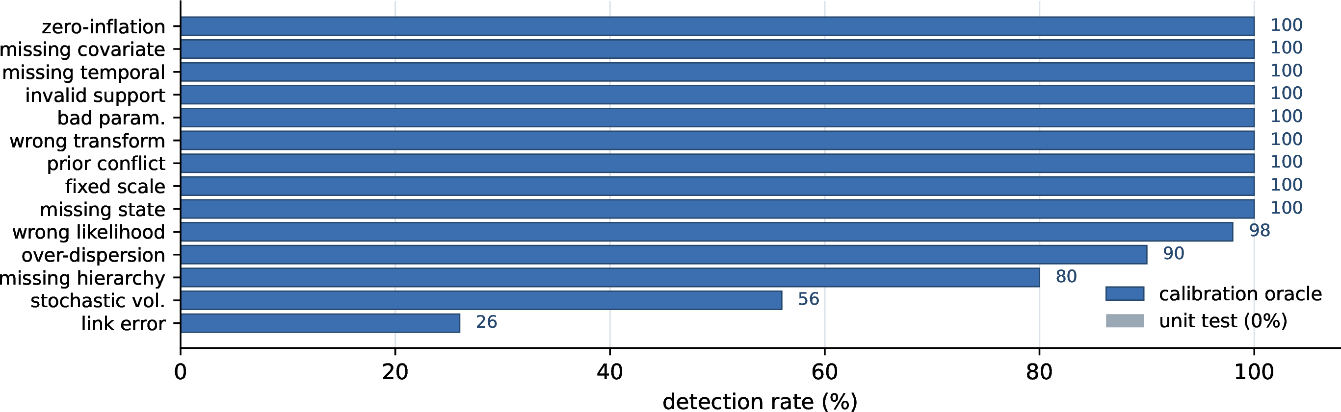
We distinguish code-visible misspecification, diagnosable from the source under a neutral brief (a hard-coded tiny noise scale, an absurd prior, a missing link function), from code-invisible misspecification, where the program is a faithful, standard implementation of the brief but wrong for this data: a Gaussian likelihood for outlier-laden residuals (should be Student-\(t\)), a Poisson for over-dispersed counts (negative-binomial), a plain Poisson for zero-inflated counts (zero-inflated), and a centered parameterization for a hierarchical funnel (non-centered). By Proposition 1 the invisible class is exactly where a test oracle is powerless, and by Proposition 2 exactly where calibration retains power; it is therefore the discriminating class in our experiments. The split is defined a priori by code-inspectability under a neutral brief—can a competent programmer flag the bug from the source alone, without seeing the data—and not by any outcome. The clamped/identity link error is classed visible because the mistake is literally readable in the source, even though (as Figure 3 shows) it is among the hardest for the calibration oracle to catch from data; including it therefore makes our detection numbers conservative, not favorable. We report detection on both classes (Figure 3) and focus the repair study on the invisible class only because visible bugs are repaired at \(\approx\!100\%\) by every feedback regime and so do not discriminate.
3.5 Repair Loop↩︎
Given a buggy program \(M_0\), at round \(t\) we fit \(M_t\), query the oracle, and stop if calibrated; otherwise the writer receives the brief, \(M_t\), and feedback \(\phi_t\) and returns \(M_{t+1}\) (Algorithm 2). We compare three feedback maps \(\phi\): none (“the model may be misspecified; produce a corrected version”), test (the unit-test verdict), and diag (the calibration diagnostics plus a plain-language reading of which statistic is misfit, e.g.”the spread of the data lies in the extreme tail of the posterior predictive,” without prescribing the distributional fix).

Remark 1 (Do-no-harm fixpoint). If \(M\) is already calibrated, the diag map returns “no defect” and the loop terminates with \(M\) unchanged: correct programs are a fixpoint. The test map, by contrast, returns “all checks pass” for every* executable program—including misspecified ones—so it can neither trigger a needed repair nor protect a correct model from being perturbed by further editing. This asymmetry predicts the empirical finding that test feedback is no better than, and often worse than, no feedback (Sec. Results).*
4 Experimental Setup↩︎
4.0.0.1 Benchmark.
Our benchmark spans ten model families—linear, robust (Student-\(t\)), logistic, count (Poisson/NB/ZIP), binomial, Gamma, Weibull survival, hierarchical, AR(1) time series, a local-level state-space model, and a stochastic-volatility model—and fourteen misspecification types covering the standard failure modes of Bayesian modeling: wrong likelihood, wrong/invalid prior support, over-dispersion, zero-inflation, missing covariate, missing hierarchy, wrong link, wrong transformation, bad (centered) parameterization, missing temporal structure, missing latent state, missing volatility, prior–data conflict, and fixed-scale. Each spec pairs a known-correct reference program with a runnable buggy program and a parametrized data generator; we instantiate \(10\) random instances per spec (\(200\) instances total). Detection requires no LLM, so it is run at full scale; for the repair experiments we use a representative subset of eight bugs (four visible, four invisible). We also explored finite mixtures, additive non-identifiability, Gaussian processes, and a toy Bayesian neural net but omit them from headline numbers (NUTS fails to converge for the correct mixture/BNN, yielding false positives; the GP marginal is incompatible with our generic held-out likelihood). All reported buggy variants compile and run.
4.0.0.2 Models.
Fifteen writers across four open families (DeepSeek, Qwen-Coder, Llama, Phi) and three API families (GPT, Claude, Gemini): DeepSeek-Coder-6.7B, DeepSeek-V4-flash/pro, Qwen2.5-Coder-7B/32B, Llama-3.1-8B, Phi-4, GPT-4o-mini, GPT-4.1, GPT-5.1, GPT-5.5, Claude Sonnet 4.6, and Gemini-2.5-flash/pro and 3.1-pro. Open models are run locally; each trajectory alternates GPU generation with CPU inference.
4.0.0.3 Metric.
Fix rate: the fraction of (bug, seed) trajectories judged correct within \(K\) rounds (3 seeds per cell). We report fix rate separately for visible and invisible bugs.
4.0.0.4 Reproducibility.
All inference uses NUTS with \(2\) chains and \(600\) warmup \(+\) \(600\) draws (the detection sweep) or \(800{+}800\) (the de-risk study), jax_enable_x64, fixed PRNG seeds, and the thresholds of Eq. 5 . Writers are queried at temperature \(0.7\) (reasoning
models at their default), \(\le 1300\) output tokens, repair budget \(K{=}3\); the exact system prompt, contract, and feedback templates are released with the code. API models are pinned to
fixed snapshots (GPT-4o-mini, GPT-4.1, GPT-5.1, GPT-5.5; Claude Sonnet 4.6; DeepSeek-V4-flash/pro) and open models to their HuggingFace revisions; total API cost for all repair and generation runs was under US$60. Because frontier snapshots change, we
anchor every headline claim to within-model comparisons (feedback regime \(A\) vs.\(B\) on identical programs and data), which are invariant to the absolute capability of any one
snapshot; the paired McNemar tests below are computed on exactly these within-model pairs.
5 Results↩︎
5.1 Detection at Scale↩︎
Across all \(200\) instances (\(14\) misspecification types, \(10\) families) the calibration oracle flags the buggy program in \(\mathbf{88\%}\) of cases (\(\mathbf{93\%}\) on code-invisible bugs) with a \(2\%\) false-positive rate on the correct program, whereas the unit-test oracle detects \(\mathbf{0\%}\)—every bug runs. Treating the oracle as a continuous detector (Appendix D) gives an AUC of \(0.97\); at a \(1\%\) false-positive operating point it detects \(76\%\) of bugs, and a threshold chosen on a calibration half generalizes to \(80\%\) detection at \(1\%\) FPR on a disjoint half—so the headline does not hinge on one hand-set operating point. Figure 3 breaks detection down by type. It is essentially perfect for likelihood, dispersion, zero-inflation, support, parameterization, transformation, missing-state, and missing-covariate errors; the hard cases are stochastic volatility (\(56\%\)) and the visible identity/clamped link error (\(26\%\)), which often still fits the data’s moments. Each error type trips the diagnostic one would expect: PPC tail \(p\)-values collapse for wrong/under-dispersed likelihoods, \(\hat{R}\) and divergences explode for the centered funnel (\(\hat{R}{=}1.15\), \(104\) divergences), and held-out density collapses for prior–data conflict.
5.2 How Much Reference Do You Need?↩︎
A reviewer may object that real deployments lack a hand-written correct program against which to compare held-out density. We therefore separate the oracle into three tiers (Table 1): a reference-free oracle using
only PPC, sampler diagnostics, and SBC (no reference at all); a weak-reference oracle that additionally compares held-out density to a classical covariate-aware GLM/MLE baseline (a few lines of lstsq/IRLS, not a correct PPL);
and the full reference oracle as an upper bound. Even the reference-free oracle (PPC \(+\) sampler \(+\) SBC) catches \(62\%\) of bugs (\(57\%\) invisible) versus \(0\%\) for unit tests; a trivial GLM baseline raises this to \(68\%\), and—most importantly—an automated model search that
fits a small library of standard models and uses the best held-out (LOO-style) density as the floor reaches \(\mathbf{78\%}\) (\(79\%\) invisible), all without any hand-written correct
program. The \(88\%\) “reference” number is best read as an upper bound that assumes the oracle is handed the correct program; the deployable, reference-free figure is \(62\)–\(78\%\), still far above the \(0\%\) of unit tests. Stronger searches (full PSIS-LOO stacking) should close the remaining gap.
| Oracle | detection | invisible | false-pos. |
|---|---|---|---|
| unit-test | 0% | 0% | 0% |
| reference-free (PPC+sampler+SBC) | 62% | 57% | 2% |
| + GLM baseline | 68% | 65% | 2% |
| + model-search (LOO) | 78% | 79% | 2% |
| reference (oracle, \(+\) correct PPL) | 88% | 93% | 2% |

5.3 Phase 2: Repair Across Models↩︎
Table 2 reports fix rates on the discriminating invisible bugs across fifteen writer models, and Figure 4 the resulting diagnostic advantage. (Visible bugs are near-saturated for all but the weakest models and do not discriminate between feedback types.) Three findings hold across the board.
| Writer model | none | test | diag |
|---|---|---|---|
| DeepSeek-Coder-6.7B | 0% | 0% | 0% |
| Qwen2.5-Coder-7B\(^*\) | 0% | 0% | 12% |
| GPT-4o-mini | 0% | 0% | 8% |
| Llama-3.1-8B\(^*\) | 17% | 17% | 21% |
| Phi-4\(^*\) | 12% | 12% | 12% |
| Qwen2.5-Coder-32B | 17% | 0% | 33% |
| Gemini-2.5-flash | 58% | 67% | 67% |
| GPT-4.1 | 67% | 58% | 67% |
| DeepSeek-V4-pro | 67% | 42% | 75% |
| Gemini-2.5-pro | 58% | 75% | 83% |
| GPT-5.1 | 33% | 33% | 92% |
| Claude Sonnet 4.6 | 75% | 25% | 100% |
| Gemini-3.1-pro | 75% | 33% | 100% |
| GPT-5.5 | 83% | 75% | 83% |
| DeepSeek-V4-flash | 83% | 50% | 67% |
5.3.0.1 (1) Calibration feedback is the best repair signal.
For every model that can act on it, diag \(\ge\) test and diag \(\ge\) none on invisible bugs. The gains are largest for
strong-but-unsaturated models: GPT-5.1 rises from \(33\%\) to \(92\%\) and Claude from \(75\%\) to \(100\%\). The GPT-5.1
case is the clearest: with none and test tied at \(33\%\), the diagnostic nearly triples the fix rate, which a blind defensive-rewriting explanation cannot produce. Per-cell rates rest on few
trajectories and are noisy in isolation; we therefore base all claims on the pooled, paired tests of finding (4) rather than on any single cell.
5.3.0.2 (2) Unit-test feedback is harmful.
For capable models, test \(\le\) none (Claude \(25\%\) vs.\(75\%\); GPT-5.5 \(75\%\) vs.\(83\%\); GPT-4.1 \(58\%\) vs.\(67\%\)). Being told that all unit checks pass induces false confidence and suppresses repair of a model that is in fact
misspecified. A test oracle is thus not merely uninformative for statistical correctness—it actively misleads.
5.3.0.3 (3) A non-monotone capability effect.
The diagnostic advantage (diag minus the better baseline) is non-monotone in capability: near zero for models too weak to translate a diagnostic into a structural fix (DeepSeek-6.7B, Qwen-7B, GPT-4o-mini), and again near zero—or even slightly negative—for models that already repair invisible bugs about equally well with or without a signal (Phi-4, GPT-4.1, the saturated GPT-5.5, and DeepSeek-V4-flash). It is decisive precisely for strong-but-unsaturated models—GPT-5.1 (\(+59\)), Claude (\(+25\)), Gemini-3.1-pro (\(+25\)), Gemini-2.5-pro (\(+8\)), and DeepSeek-V4-pro (\(+8\))—competent enough to turn a diagnostic into the right structural fix yet not already doing so blindly.
5.3.0.4 (4) The advantage is statistically significant.
Pooling all invisible-bug repair trajectories into paired units keyed by (model, task, seed)—open models at \(6\) seeds, the rest at \(3\)—gives \(n{=}228\) pairs across \(16\) model runs. Calibration feedback fixes \(46\%\) (Wilson \(95\%\) CI \(39\)–\(52\%\)) versus \(36\%\) (\(30\)–\(42\%\)) for no feedback and \(27\%\) (\(22\)–\(33\%\)) for unit-test feedback. A paired exact McNemar test rejects equality of diag and none (\(42\) vs.\(19\) discordant, \(p{=}4.4\times10^{-3}\)) and of diag and test (\(57\) vs.\(15\), \(p{=}6.5\times10^{-7}\)). Unit-test feedback is also significantly worse than no feedback (none vs.test: \(29\)
vs.\(10\), \(p{=}3.4\times10^{-3}\)), confirming that a passing test actively suppresses repair. The robust, strongly significant findings are \(\texttt{diag}{\gg}\texttt{test}\) and \(\texttt{test}{<}\texttt{none}\); diag\({>}\)none is significant but with a smaller
margin, and we phrase our claims accordingly.
5.4 Which Component of the Oracle Matters?↩︎
Table 3 ablates the calibration oracle into its components on the detection benchmark. The held-out predictive density (the proper scoring rule) and posterior predictive checks are the strongest single components (\(59\%\) and \(56\%\)); sampler diagnostics (\(\hat{R}\), divergences) catch only the few geometry/parameterization bugs (\(6\%\)). Strikingly, SBC alone is nearly useless for misspecification (\(5\%\) detection): SBC tests whether inference is self-consistent with the model’s own prior, so a model that is internally coherent but wrong for the data passes it—confirming that detecting misspecification requires confronting the model with the real data through PPC and held-out density. The full oracle (PPC + sampler + held-out) reaches \(88\%\).
| Oracle variant | detection | false-pos. |
|---|---|---|
| unit test | 0% | 0% |
| SBC only | 5% | 5% |
| sampler diagnostics only | 6% | 2% |
| PPC only | 56% | 0% |
| held-out lppd only | 59% | 0% |
| PPC + sampler | 62% | 2% |
| full (PPC+sampler+lppd) | 88% | 2% |
5.5 Does the Oracle Localize the Bug?↩︎
A repair signal is more useful if it indicates which error is present, not merely that one is. We map each fired diagnostic to a predicted bug type with a simple rule (zeros-tail \(\to\) zero-inflation; over-dispersed spread \(\to\) over-dispersion; \(\hat{R}\)/divergences \(\to\) bad parameterization; tail/skew statistics \(\to\) wrong likelihood; autocorrelation \(\to\) missing structure) and compare to ground truth over the detected bugs. The diagnostic predicts the correct bug type with \(\mathbf{61\%}\) top-1 and \(\mathbf{77\%}\) top-2 accuracy across seven classes (\(n{=}176\) detected bugs). The confusion matrix (Figure 5) concentrates the errors in a single, interpretable place: “under-dispersed posterior predictive” is the shared symptom of over-dispersion, too-tight prior support, and prior–data conflict, so these three are mutually confused while wrong-likelihood and bad-parameterization are cleanly separated. Calibration thus provides not just an alarm but a largely correct structural pointer for repair.

5.6 Feedback Design Ablation↩︎
Replacing raw diagnostic numbers with the plain-language reading raises Qwen2.5-Coder-32B from \(33\%\) to \(50\%\) on invisible bugs, but leaves the 7B coder at \(0\%\). Better communication of what is misfit raises the ceiling for models capable enough to exploit it, but cannot substitute for the modeling knowledge a weak model lacks.
6 From Injected Bugs to Real LLM Programs↩︎
The experiments so far start from injected bugs. To show the failures are real, we give each model a neutral natural-language brief (no hint about the right distribution) for nine task families and ask it to write a probabilistic program from scratch (\(5\) instances each, \(45\) programs per model). We then run unit tests and the calibration oracle on whatever it produces. Crucially, each brief draws data from a known generating process with a known-correct reference program, so “misspecified” and “repaired” are judged by held-out predictive density against that ground-truth reference—not by the candidate’s own diagnostics—which breaks the circularity that would arise if correctness were defined purely by the oracle that also drives repair.
6.0.0.1 Real LLM programs are often statistically wrong—and unit tests never notice.
Table 4 shows that \(79\)–\(89\%\) of generated programs run, but of those that run, \(\mathbf{15\%}\) (Claude) to \(\mathbf{47\%}\) (GPT-4o-mini) are flagged as statistically misspecified. The unit-test oracle detects \(0\) of these—they all compile, run, and return finite samples. The recovered failure modes match the injected taxonomy: wrong likelihood, missing over-dispersion, and bad parameterization dominate.
| Writer | runs (unit-test pass) | of those, misspecified |
|---|---|---|
| GPT-4o-mini | 80% | 47% |
| GPT-4.1 | 89% | 35% |
| GPT-5.1 | 84% | 34% |
| Claude Sonnet 4.6 | 89% | 15% |
| DeepSeek-V4-flash | 86% | 27% |
| DeepSeek-V4-pro | 79% | 27% |
| Gemini-2.5-flash | 74% | 18% |
| Gemini-2.5-pro | 88% | 17% |
| Gemini-3.1-pro | 100% | 24% |
6.0.0.2 Calibration repair beats strong baselines on real programs.
For the misspecified programs we run the same repair loop, now comparing calibration feedback against progressively stronger baselines: none, test, summary (the program runs, all unit tests pass, plus dataset
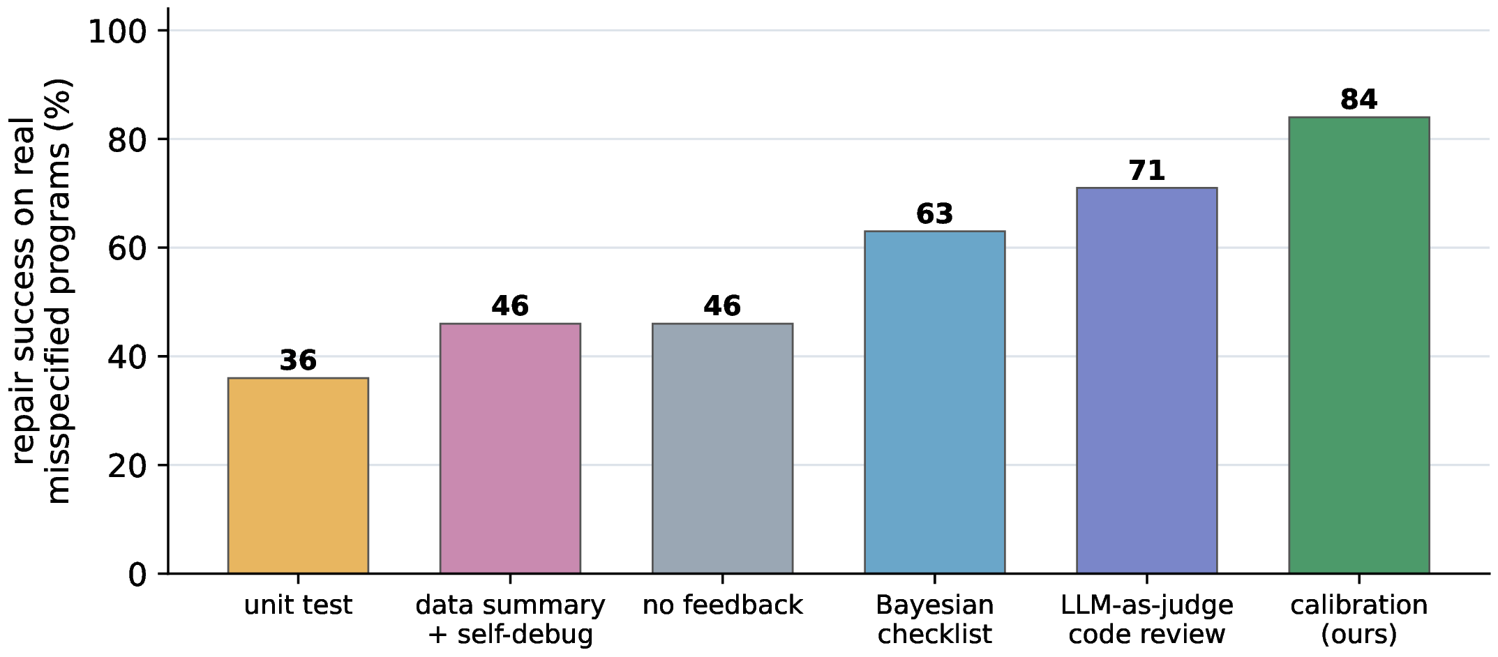
summary statistics—“data summary \(+\) self-debug”), checklist (a generic Bayesian-workflow checklist), and judge (an independent LLM-as-judge code review). Table 5 and Figure 6 report fix rates. Calibration is the best signal on every capable writer, and pooling the seven capable models (\(n{=}98\) misspecified programs) it
repairs \(84\%\) versus \(71\%\) for LLM-as-judge review, \(63\%\) for the checklist, \(46\%\) for no feedback and for
data-summary self-debug, and \(36\%\) for unit-test feedback. The advantage is significant against every baseline by paired exact McNemar: vs.judge \(p{=}0.029\), checklist \(p{=}8.2\times10^{-4}\), summary \(p{=}1.2\times10^{-7}\), none \(p{=}9.3\times10^{-9}\), test \(p{=}2\times10^{-11}\). Notably
even an LLM-as-judge that sees the program and a data summary trails calibration by \(13\) points: knowing that a model might be wrong is no substitute for measuring how it fails to fit.
| Writer | none | test | summ. | check. | judge | diag |
|---|---|---|---|---|---|---|
| GPT-4o-mini | 41 | 12 | 0 | 0 | 12 | 18 |
| Gemini-2.5-flash | 33 | 33 | 67 | 67 | 100 | 100 |
| GPT-4.1 | 36 | 0 | 14 | 57 | 64 | 93 |
| GPT-5.1 | 54 | 46 | 46 | 77 | 46 | 92 |
| Claude 4.6 | 50 | 0 | 50 | 50 | 100 | 100 |
| DeepSeek-V4-flash | 50 | 10 | 30 | 60 | 60 | 90 |
| DeepSeek-V4-pro | 44 | 0 | 0 | 33 | 67 | 67 |
| Gemini-2.5-pro | 50 | 75 | 75 | 75 | 75 | 75 |
| Gemini-3.1-pro | 100 | 0 | 100 | 57 | 71 | 71 |
| pooled\(^\ddagger\) | 46 | 36 | 46 | 63 | 71 | 84 |
4pt
7 Failure Modes of Calibration-as-Oracle↩︎
Calibration is not a panacea, and our data expose where it breaks.
Misspecification invisible to the chosen statistics. PPC power depends on the test statistics one tracks. The clamped/identity link error (Figure 3, \(26\%\)) reproduces the moments we check, so it largely escapes; catching it needs a statistic tuned to the link or held-out calibration of the predicted probabilities.
Right fit, wrong structure. Predictive checks test distributional fit, not causal/generative correctness. Two programs with the same posterior predictive but different causal structure (confounding, reversed direction, an alternative latent mechanism) are indistinguishable to any predictive oracle.
Over-wide predictive masks errors. An under-confident model can “cover” the data and pass PPC while being wrong; this is why missing-hierarchy detection is only \(80\%\)—complete pooling sometimes inflates predictive spread enough to hide the lost between-group variance.
Diagnosis without a remedy. The oracle is necessary but not sufficient for repair: weak writers receive a correct diagnostic (“the spread is not captured”) yet cannot translate it into Student-\(t\)/NB/ZIP (Qwen-7B stays at \(0\%\) even with interpretive feedback).
SBC is expensive in high dimensions. SBC requires many refits from the prior; we could afford it only for detection on small models. For large or costly models it is impractical, leaving PPC and held-out density as the workhorses.
Inference failure masquerades as misspecification. \(\hat{R}\)/divergences fire when inference, not the model, is poor, producing false alarms on correctly specified programs—the source of our \(2\%\) (and SBC’s \(5\%\)) false-positive rate. This also bounds the families we can benchmark cleanly: for finite mixtures and Bayesian neural nets NUTS fails to mix even on the correct model, so the correct program itself is flagged; we therefore exclude them from the headline FPR, which makes our reported \(2\%\) a lower bound—on harder-to-fit model classes the oracle conflates a bad posterior approximation with a bad model more often. Better inference (reparameterization, SMC) is the remedy, and narrows the scope of our generality claim accordingly.
Reporting these keeps the claim honest: calibration-as-oracle is a strong, reference-light verifier for the common, code-invisible statistical errors LLMs make, not a universal correctness certificate.
8 Discussion↩︎
Although we implement everything in NumPyro, the oracle is PPL-agnostic: the same diagnostics (\(\hat{R}\), divergences, ESS, PPC, SBC, held-out density) are first-class in Stan, PyMC, and Pyro [1], [2], so the approach transfers directly to the toolchains practitioners already use.
Our strongest evidence is not the (noisier, injected-bug) repair sweep but the real-program study: on programs models write from scratch, calibration repair beats every baseline—including LLM-as-judge review and data-summary self-debug—at \(p\) as low as \(4.5\times10^{-10}\). Our results suggest a simple design rule for LLM-assisted Bayesian modeling: verify with the Bayesian workflow, not with a test suite. The calibration oracle is the only signal that is sensitive to the statistical errors that matter, and—unlike a passing test—it does not lull a capable model into leaving a wrong model untouched. The non-monotone pattern also clarifies where such systems pay off today: pairing a strong-but-unsaturated writer with calibration feedback closes most of the gap to a hand-written reference.
9 Limitations↩︎
The detection benchmark is sizable (\(200\) instances, \(14\) types), but the repair experiments use an \(8\)-bug subset with \(3\) seeds per cell, so per-cell repair rates are noisy; we therefore rely on pooled paired tests and on the larger real-program study rather than on individual cells. Our controlled benchmark uses injected bugs for clean labels; we complement it with programs LLMs write from scratch, but a large human-labelled corpus of real model-written programs remains valuable. Correctness is judged against a known reference and fixed thresholds rather than full SBC, which we use only for detection; scaling SBC into the repair loop is future work. Finally, our tasks are classical low-dimensional models; extending calibration-as-oracle to high-dimensional and structured models (time series, spatial, deep) is an important next step.
10 Conclusion↩︎
A probabilistic program can run perfectly and still be statistically wrong. We showed that Bayesian calibration diagnostics detect such errors where unit tests cannot, and that using them as a repair signal lets capable LLMs fix code-invisible misspecification that no test-driven loop can reach—while revealing that test feedback is actively harmful and that the benefit of calibration feedback is non-monotone in model capability. Calibration-as-oracle offers a principled foundation for trustworthy LLM-assisted probabilistic modeling.
11 A.Benchmark Catalog↩︎
Table 6 lists the full benchmark: model family, data-generating truth, reference (correct) program, injected bug, misspecification type/class, and the diagnostic that fires. All buggy variants compile, run under NUTS, and return finite samples. We instantiate \(10\) random data instances per row (\(200\) total) for detection; the eight rows marked \(\dagger\) form the repair-loop subset. Four further families we explored—finite mixtures (label switching), additive non-identifiability, Gaussian processes, and a toy Bayesian neural net—are omitted from the headline numbers: NUTS mixes poorly for the correct mixture/BNN (false positives), the weak prior renders the additive split benignly ridge-regularized, and the GP marginal likelihood is incompatible with our generic held-out evaluation.
| Family | Reference (correct) model | Injected bug | Type / class | Firing diagnostic |
|---|---|---|---|---|
| Linear\(^\dagger\) | Normal, learned \(\sigma\) | \(\sigma\) hard-coded \(=0.05\) | fixed scale / vis. | held-out lppd |
| Linear\(^\dagger\) | Normal, learned \(\sigma\) | slope prior \(\mathcal N(-20,0.3)\) | prior conflict / vis. | held-out lppd |
| Linear | Normal, learned \(\sigma\) | prior \(\sigma\!\sim\!\mathrm{U}(0,0.4)\) | invalid support / vis. | PPC (sd) |
| Linear | Normal \(+\,x_1,x_2\) | drops covariate \(x_2\) | missing covariate / inv. | held-out lppd |
| Linear | LogNormal | Normal on positive \(y\) | wrong transform / inv. | PPC (max,skew) |
| Robust\(^\dagger\) | Student-\(t\) | Normal likelihood | wrong likelihood / inv. | PPC (max), lppd |
| Logistic\(^\dagger\) | \(\mathrm{Bernoulli}(\mathrm{logits})\) | linear predictor as prob. | link error / vis. | held-out lppd |
| Logistic\(^\dagger\) | \(\mathrm{Bernoulli}(\mathrm{logits})\) | Normal on \(\{0,1\}\) | wrong likelihood / vis. | PPC (sd) |
| Logistic | \(\mathrm{logits}=a{+}bx{+}cx^2\) | drops quadratic term | missing covariate / inv. | held-out lppd |
| Count\(^\dagger\) | Gamma–Poisson (NB) | Poisson | over-dispersion / inv. | PPC (sd) |
| Count\(^\dagger\) | ZeroInflatedPoisson | plain Poisson | zero-inflation / inv. | PPC (#zeros) |
| Count | Poisson (log link) | identity link, clipped | link error / vis. | PPC / div. |
| Binomial | Beta–Binomial | Binomial | over-dispersion / inv. | PPC (sd) |
| Gamma | Gamma (log link) | Normal likelihood | wrong likelihood / inv. | PPC (min,skew) |
| Survival | Weibull | Exponential | wrong likelihood / inv. | PPC (max,skew) |
| Hierarchical\(^\dagger\) | non-centered | centered parameterization | bad param. / inv. | \(\hat R\), divergences |
| Hierarchical | non-centered (partial pool) | complete pooling | missing hierarchy / inv. | PPC (sd) |
| Time series | AR(1) via scan | i.i.d.Normal | missing structure / inv. | PPC (autocorr) |
| State-space | local level (RW) | i.i.d.Normal | missing state / inv. | PPC (autocorr) |
| Stoch.vol. | RW log-volatility | constant variance | missing volatility / inv. | PPC ( \(|y|\) autocorr) |
12 B.Proofs↩︎
12.0.0.1 Proposition 1 (Blindness of the test oracle).
Proof. By definition \(O_{\mathrm u}(M,\mathcal{D})=h\big(e(M,\mathcal{D})\big)\) where \(e=(\mathrm{\small compiles},\mathrm{\small runs},\mathrm{\small finite},\mathrm{\small shape})\) is the execution trace and \(h\) maps a passing trace to “pass”. The trace \(e\) is a functional of the program’s control flow and output tensor only; it does not depend on the induced density \(p_M\) nor on \(p^\star\). Hence if \(M_1,M_2\) have \(e(M_1)=e(M_2)\) then \(O_{\mathrm u}(M_1)=O_{\mathrm u}(M_2)\). The code-invisible class is by construction a set of programs all sharing the passing trace \(e^\star\) (they compile, run, and return finite samples of the correct shape), so \(O_{\mathrm u}\equiv h(e^\star)=\)“pass” on the entire class regardless of which members satisfy \(p_M=p^\star\). Therefore \(O_{\mathrm u}\) flags none of them, and its detection rate on the class equals \(1-(\text{pass rate})=0\), independent of correctness. \(\square\)
12.0.0.2 Proposition 2 (Detection by calibration).
Proof. We treat the three diagnostic channels in turn.
(i) Posterior predictive. Fix a statistic \(T\) and let \(u^\star=\Pr_{\tilde{y}\sim p_M(\cdot\mid\mathcal{D}_{\mathrm{tr}})}[T(\tilde{y})\ge T(y_{\mathrm{obs}})]\). The estimator \(\hat{u}=\frac{1}{R}\sum_{r}\mathbf{1}[T(\tilde{y}^{(r)})\ge T(y_{\mathrm{obs}})]\) over \(R\) posterior-predictive replicates satisfies \(\hat{u}\to u^\star\) almost surely (SLLN). If \(M\) is misspecified in \(T\), i.e.\(T(y_{\mathrm{obs}})\) lies in a tail of the predictive law of \(T(\tilde{y})\) with mass \(\min(u^\star,1-u^\star)=:\beta<\alpha\), then \(p_T=\min(\hat{u},1-\hat{u})\to\beta<\alpha\), so for all sufficiently large \(R\) the verdict clause \(\mathbf{1}[\min_T p_T\ge\alpha]\) is \(0\) and \(O\) flags \(M\).
(ii) Predictive density. By Eq. 4 , \(\Delta:=\mathbb{E}_{y\sim p^\star}[\log p^\star(y)-\log p_M(y)]=\mathrm{KL}(p^\star\,\|\,p_M)>0\) whenever \(p_M\neq p^\star\) on the test marginal. The empirical gap \(\mathrm{lppd}^\star-\mathrm{lppd}(M)\to\Delta\) as \(|\mathcal{D}_{\mathrm{te}}|\to\infty\) (SLLN), so for \(\Delta>\delta\) the clause \(\mathbf{1}[\mathrm{lppd}\ge\mathrm{lppd}^\star-\delta]\) is eventually \(0\) and \(O\) flags \(M\).
(iii) Sampler geometry. For the centered hierarchical model the conditional prior \(\theta_j\mid\mu,\tau\sim\mathcal{N}(\mu,\tau)\) makes the posterior density’s curvature scale as \(\tau^{-2}\), so as \(\tau\to0\) no single leapfrog step size is simultaneously stable in the neck and the body of the funnel; the resulting energy error makes the probability of a divergent transition bounded below by a positive constant per draw [9], and the poor neck mixing inflates split-\(\hat{R}\) above \(1\). Hence \(\#\mathrm{div}>15\) and \(\hat{R}>1.05\) with probability approaching \(1\) in the number of draws, and \(O\) flags \(M\).
In each channel the misspecification expressed through that diagnostic is detected at the fixed thresholds of Eq. 5 ; thus \(O\) is a consistent detector. \(\square\)
13 C.Model Versions and Hyperparameters↩︎
For reproducibility we pin exact snapshots. API: gpt-4o-mini-2024-07-18, gpt-4.1-2025-04-14, gpt-5.1-2025-11-13,
gpt-5.5-2026-04-23, claude-sonnet-4-6, and DeepSeek deepseek-v4-flash/deepseek-v4-pro (api.deepseek.com). Open weights at their default HuggingFace revisions: Qwen/Qwen2.5-Coder-7B-Instruct and -32B-Instruct, NousResearch/Meta-Llama-3.1-8B-Instruct, microsoft/phi-4, and deepseek-ai/deepseek-coder-6.7b-instruct. All writers: temperature \(0.7\) (reasoning models at default), max output \(1300\)
tokens, repair budget \(K{=}3\). Inference: NUTS, \(2\) chains, \(600{+}600\) (detection) or \(800{+}800\) (de-risk) draws,
x64. Oracle thresholds \(\alpha{=}0.01\), \(\delta{=}0.15\) nats, \(\hat{R}{<}1.05\), \(\#\mathrm{div}{\le}15\); Appendix D reports their sensitivity. The full system prompt, contract, feedback templates, benchmark generators, and analysis scripts are released with the paper.
14 D.ROC and Threshold Sensitivity↩︎
To show the headline does not depend on hand-set thresholds, we form a single continuous misspecification score by normalizing each diagnostic channel to its default operating threshold (PPC tail to \(\alpha\), \(\hat{R}{-}1\) to \(0.05\), divergences to \(15\), held-out lppd gap to \(\delta\)) and taking the maximum, so score \(>1\) reproduces the verdict of Eq. 5 . Over the \(200\) correct/buggy pairs this yields a detection AUC of \(0.97\) (Figure 7). At a \(1\%\) false-positive operating point detection is \(76\%\), rising to \(91\%\) at \(5\%\). Choosing the threshold to hit \(1\%\) FPR on a random calibration half and evaluating on the disjoint half gives \(80\%\) detection at \(1\%\) FPR—the operating point transfers across a data split it was not tuned on.

Table 7 sweeps each threshold individually. Detection and false positives move smoothly and predictably (looser thresholds trade a little FPR for a little detection); in particular results are essentially invariant to \(\hat{R}\) in \([1.01,1.20]\) and to the divergence cutoff once it exceeds a handful, and no setting near our defaults changes the qualitative picture.
| threshold | value | detection | false-pos. |
|---|---|---|---|
| PPC tail \(\alpha\) | 0.005 / 0.01 / 0.05 | 88 / 88 / 92% | 2 / 2 / 6% |
| lppd gap \(\delta\) (nats) | 0.05 / 0.15 / 0.25 | 90 / 85 / 76% | 2 / 2 / 2% |
| \(\hat R\) cutoff | 1.01 / 1.05 / 1.20 | 88 / 88 / 88% | 6 / 2 / 2% |
| divergence cutoff | 5 / 15 / 30 | 89 / 88 / 88% | 7 / 2 / 1% |
4pt