Fully Automated High-Precision Segmentation of Retinal Atrophy and Ellipsoid Zone Thickness in OCT: A Reliable Tool for Real-World GA Monitoring.
June 30, 2026
Abstract
Geographic atrophy (GA) secondary to age-related macular degeneration (AMD) requires precise monitoring of relevant structural biomarkers to assess disease stage, progression, and treatment response. This paper presents a fully automated, deep learning-based framework for the high-precision, pixel-wise segmentation of key biomarkers in optical coherence tomography (OCT) imaging: retinal pigment epithelium (RPE) loss, ellipsoid zone (EZ) loss, and EZ thinning. The proposed pipeline uses three specialized semantic segmentation models to delineate RPE loss, EZ boundaries (including interruptions), and Bruch’s membrane. To ensure robustness and generalizability, the models were developed on a diverse dataset of 298 SD-OCT volumes representing the full phenotypic spectrum of AMD (GA:222, intermediate AMD: 40, neovascular AMD: 17, healthy: 19) and validated on an independent external dataset (n=43). The comprehensive evaluation was further strengthened using additional datasets to assess repeatability, inter-reader reliability, the impact of B-scan density on measurement accuracy, and subgroup performance stratified by lesion size. Results demonstrated high segmentation accuracy (Dice RPE loss: \(0.88\), Dice EZ loss: \(0.87\), Pearson’s r \(> 0.99\)). Total EZ thickness measurements exhibited a sub-pixel average deviation of \(2.15 \si{\micro\metre}\), and segmentation reliability was confirmed by a strong reproducibility score (ICC \(> 0.98\)). By accurately and consistently quantifying outer photoreceptor degeneration and RPE loss, this fully automated framework provides a highly reliable tool for GA assessment in both clinical trials and routine real-world ophthalmic care.
1 Introduction↩︎
Age-related macular degeneration (AMD) remains a leading cause of irreversible visual impairment worldwide, particularly within aging demographics [@chakravarthyCharacterizingDiseaseBurden2018]. GA represents the advanced "dry" stage of AMD, characterized by progressive loss of RPE, overlying PRs, and the underlying choriocapillaris [@holzGeographicAtrophyClinical2014]. The expanding lesions compromise the macula’s functional integrity, leading to scotoma and irreversible practical blindness. In clinical practice, OCT has meanwhile superseded fundus autofluorescence as the gold standard for diagnosing and monitoring GA [@reiterAIClinicalManagement2024]. By providing high-resolution, cross-sectional visualizations of retinal microlayers, OCT enables a precise demarcation of atrophic boundaries. In OCT imaging, GA is primarily identified by the attenuation of PR-related structures, RPE degeneration, and a subsequent increase in choroidal hypertransmission [@saddaConsensusDefinitionAtrophy2018].
Functional decline in GA is primarily driven by PR atrophy. While RPE loss is often the most prominent clinical marker, PR survival depends strongly on the metabolic support provided by the underlying RPE. Recent longitudinal studies have highlighted that photoreceptor thinning and disruption consistently precede the loss of the RPE layer [@zekavatPhotoreceptorLayerThinning2022]. In morphological imaging, the EZ is the primary OCT biomarker for monitoring PR integrity. The EZ appears as a hyperreflective layer, located immediately above the RPE, representing the mitochondria-rich compartment of the photoreceptor outer segments. EZ thickness and integrity has been shown to be a highly relevant biomarker correlating with retinal function, disease progression rate, and treatment response [@reiterSubretinalDrusenoidDeposits2020; @pfauProgressionPhotoreceptorDegeneration2020; @riedlEffectPegcetacoplanTreatment2022; @voglPredictingTopographicDisease2023; @maresCorrelationRetinalFluid2025; @birnerStructureFunctionCorrelationDeepLearning2025; @birnerNormativeProspectiveData2025; @maiDynamicsEZRPE2025]. This clinical significance was recently solidified by the FDA, which has started to recognize EZ integrity as a formal structural endpoint in GA clinical trials [@stealthbiotherapeuticsinc.ReNEWPhase32025].
Manual segmentation of GA lesions and the quantification of EZ integrity are labor-intensive tasks, rendering the process impractical for routine clinical workflows. Manual segmentation of a pathological and low-reflectance layer is also affected by subjective variability. Recent advancements in automated DL algorithms - specifically CNNs - have enabled high-throughput, objective segmentation of the biomarkers RPE loss [@ruiz-morenoAutomaticQuantificationSoftware2020; @lachinovProjectiveSkipConnectionsSegmentation2021; @pramilDeepLearningModel2023; @moranoDeepMultimodalFusion2024; @spaideEstimatingUncertaintyGeographic2025; @al-khersanDeepLearningBasedSegmentation2025] and EZ degradation [@orlandoAutomatedQuantificationPhotoreceptor2020; @pfauProgressionPhotoreceptorDegeneration2020; @kalraAutomatedIdentificationSegmentation2023; @schmidt-erfurthDiseaseActivityTherapeutic2025; @birnerExploringTrialEndpoints2026]. However, a significant limitation is that many of these models are trained on curated clinical trial data with strict inclusion and exclusion criteria, such as specific lesion size ranging. This reliance on "clean" data may compromise the generalizability and performance of these models when applied to diverse, real-world clinical populations [@suNavigatingDistributionShifts2025].
In this work, we present a fully automated DL framework for the pixel-wise segmentation of RPE loss, EZ layer loss, and EZ thinning using an ensemble of CNNs. To ensure high generalizability, the models were trained on a diverse dataset comprising both clinical trial and real-world data, spanning the full spectrum of the disease: from early-onset to late-stage GA, as well as iAMD, nAMD, and healthy controls. The method has been validated on an independent real-world dataset. Furthermore, our evaluation was strengthened by adding (1) a stratified analysis by lesion size, (2) a reproducibility study, (3) an inter-reader reliability assessment, and (4) an analysis of the relevance of OCT B-Scan density on RPE loss and EZ loss computation, comprehensively confirming the accuracy and reliability of fully automated biomarker quantification in OCT imaging.
2 Methods↩︎
2.1 Data acquisition↩︎
All SD-OCT scans have been acquired on a Spectralis device (Heidelberg Engineering GmbH, Heidelberg, Germany). The development dataset comprised SD-OCT volumes sourced from three distinct cohorts. These included: (1) the FILLY Phase-II clinical trial [@liaoComplementC3Inhibitor2020] (NCT02503332); (2) a multi-device study from the Macula Clinic at the Medical University of Vienna (MUV), featuring patients with iAMD and GA [@kostolnaSystematicProspectiveComparison2024]; and (3) a subset of iAMD and GA cases from the Vienna Imaging Biomarker Eye Study (VIBES) real-world registry [@gerendasVALIDATIONAUTOMATEDFLUID2022]. An additional independent validation dataset was assembled using separate scans from VIBES, ensuring that development and validation sets were mutually exclusive at the patient level. For the reproducibility study, data were utilized from the OAKS and DERBY Phase-III clinical trials [@heierPegcetacoplanTreatmentGeographic2023] (NCT03525613 and NCT03525600). For the B-scan density analysis, a SD-OCT dataset with dense B-scan sampling (193 B-scans per volume) of patients with GA has been incorporated [@tratnig-franklAutomatedOCTtailoredBiomarker2025]. All studies adhered to the Declaration of Helsinki, with informed consent obtained from all participants. Scans were fovea-centered with patterns ranging from \(49\times512\) to \(97\times1024\) (B-scans \(\times\) A-scans), covering an approximate \(6\times6 \si{\milli\metre}\) (\(20°\)) field of view.
2.2 Data preparation↩︎
2.2.0.1 Data selection:
To ensure model robustness, the development set (n=298 eyes) was curated for maximum phenotypic variability. This included a broad range of lesion sizes, edge cases challenging prior automated segmentation iterations [@lachinovProjectiveSkipConnectionsSegmentation2021], and non-GA controls. The latter encompassed iAMD featuring iRORA [@saddaConsensusDefinitionAtrophy2018] and drusen, nAMD with associated retinal fluid and subretinal fibrosis, and healthy eyes with normal aging phenotypes.
For the validation cohort, 43 scans were selected from 950 eyes with confirmed GA in the VIBES registry using stratified random sampling based on RPE loss area and drusen volume. Drusen volume was quantified using a previously validated in-house segmentation model.
The reproducibility dataset consisted of paired screening and baseline scans from the OAKS and DERBY trials. Selection was restricted to treatment-naïve eyes with an inter-visit interval of less than 10 days to avoid relevant GA progression [@coulibalyProgressionDynamicsEarly2023a]. Furthermore, baseline scans had to be spatially registered to their respective screening volumes to ensure anatomical alignment.
2.2.0.2 Annotation of development and validation dataset:
Ground truth was established by four experienced graders according to a clinically validated protocol. RPE loss was defined as the complete absence of the EZ band, downward displacement (subsidence) of the ONL and OPL, and substantial irregularities or absence of the typically continuous hyperreflective RPE band. While choroidal hypertransmission was used to localize atrophic lesions, it was not used for the final delineation of boundaries. There was no minimum size restriction regarding the GA loss area. Graders also delineated retinal and subretinal layers, precisely the BM, IB-EZ, and OB-OPR. The latter is commonly identical to the inner boundary of the RPE layer, except in presence of subretinal fluid, or deposits such as SDD, fibrotic tissue or blood. In that case OB-OPR is delineated above these materials. EZ loss was identified by any interruption in the EZ band, including focal disruptions caused by SDD or pigment migration. A manual annotation example is provided in Fig. 1.

For 49-slice volumes, RPE loss was annotated on every B-scan, while higher-density volumes were sampled at every second B-scan. The EZ layer was annotated with a lower density, processing every fifth B-scan for 49-slice volumes and every tenth B-scan for higher-density volumes.
To optimize efficiency, annotators performed manual refinement of initial automated segmentations generated by previously described algorithms[@lachinovProjectiveSkipConnectionsSegmentation2021; @orlandoAutomatedQuantificationPhotoreceptor2020] for the development dataset. The validation dataset was annotated de-novo (from scratch), to avoid bias from automated segmentation.
Quality was maintained through standardized weekly consensus meetings with a supervisor and a senior retinal specialist. Final validation segmentations consistently underwent additional oversight by a retinal specialist. All layer boundary and loss area annotations were performed using a proprietary, pixel-accurate manual software developed at the Medical University of Vienna previously.
To prevent data leakage, the validation set was not utilized for model training or hyperparameter tuning. Developers only gained access to the validation annotations after full completion of model development.
2.3 Model training↩︎
Three semantic segmentation models were developed to segment RPE loss, EZ and BM layer boundaries on SD-OCT scans (Fig. 2). BM segmentation was utilized to flatten the retinal curvature, providing a normalized input for the subsequent RPE loss model. During post-processing, outputs from all three models were integrated to generate the final segmentation and compute relevant biomarkers. 2D architectures were sourced from the PyTorch Image Models (TIMM) library [@rw2019timm], while the 3D-to-2D model was based on three candidate models evaluated by Morano et al. [@moranoSelfsupervisedLearningIntermodal2023]. Final architectures and hyperparameters were selected based on peak performance during validation set experiments.
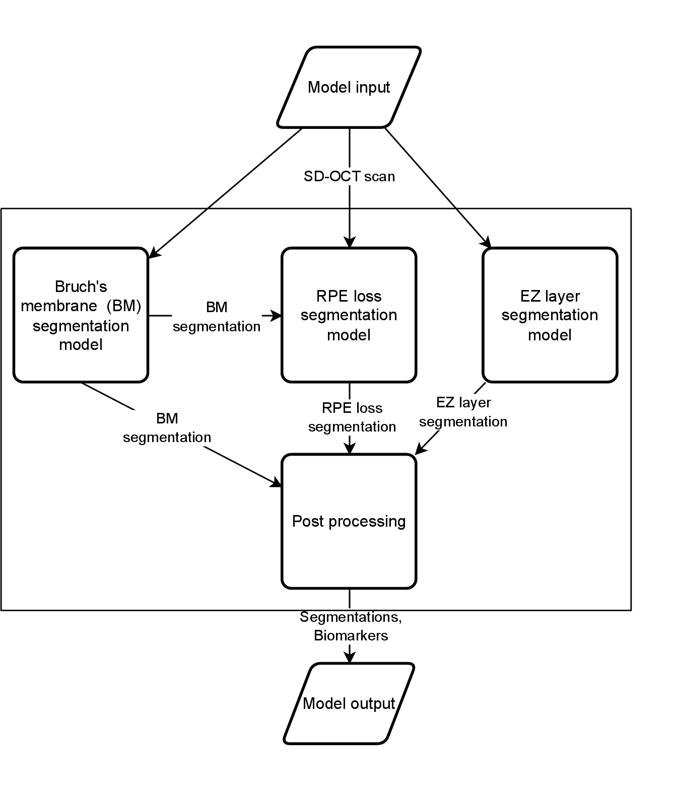
2.3.0.1 BM segmentation model
BM segmentation was implemented using the SD-Layernet framework [@fazekasSegmentationBruchsMembrane2023; @fazekasSDLayerNetSemisupervisedRetinal2022], leveraging a topological engine to incorporate anatomical priors. We employed a 2D CNN UNet++ [@zhouUNetRedesigningSkip2020] featuring an EfficientNet-B5 encoder [@tanEfficientNetRethinkingModel2019] to predict BM positions per individual A-scan at subpixel resolution. Training involved diverse stochastic augmentations: spatial shifts (zoom, left-right flip, translation, tilting, and bending), noise injection (speckle, Gaussian), intensity variations (linear and non-linear contrast changes, contrast gradients, artificial vessel shadows). The model was optimized via a composite loss function comprising DSC and CE for layer masks, MAE for layer positions, and topological constraints for curvature and continuity [@fazekasSDLayerNetSemisupervisedRetinal2022; @fazekasSegmentationBruchsMembrane2023]. Training was conducted for 80 epochs using the Adam optimizer (LR=\(2\times10^{-4}\)), with the final model selected based on the lowest validation MAE. Development dataset splitting followed a 76:12:12 ratio (train/val/test), grouped by patient and stratified by RPE loss area and disease label.
2.3.0.2 EZ layer segmentation model
The EZ was segmented using a 2D U-Net architecture featuring a DenseNet-201 encoder [@huangDenselyConnectedConvolutional2017]. Segmentation masks were defined across three distinct anatomical regions: from the IB-EZ to the OB-OPR, from the OB-OPR to BM, and from BM to the bottom of the B-scan. The model was trained for 80 epochs via the Adam optimizer (LR=\(1.8\times10^{-4}\), weight decay = \(3\times10^{-5}\)). Final model selection was based on a weighted DSC metric (0.3 for the EZ region and 0.7 for EZ interruptions). The dataset split and the stochastic augmentations remained identical to the BM segmentation.
2.3.0.3 RPE loss segmentation model
RPE loss was segmented using a 3D-to-2D FPN [@moranoSelfsupervisedLearningIntermodal2023], which transforms a full 3D OCT volume into a 2D en-face segmentation map. To reduce spatial variance and standardize the input, each scan was first flattened relative to BM using the segmentation output from the BM model. A-scans were vertically shifted to center the BM layer in the B-scan. Stochastic training augmentations were consistent with those used in other models, excluding tilt/bend transforms that are obsolete in flattened images, and the addition of random spatial cropping and B-scan order flipping. The model was trained using a balanced composite loss (0.5 DSC and 0.5 CE) optimized via SGD (LR=\(0.05\), momentum =\(0.85\), weight decay =\(3.5\times10^{-4}\)). We implemented a "Reduce Learning Rate on Plateau" scheduler with a patience of 150 epochs, a 20-epoch cooldown, and a 0.5 reduction factor. Each model within the cross-validation framework was trained for 500 epochs using 16-bit mixed precision and a batch size of 16. Model selection was based on the mean DSC score for RPE loss. The development dataset was partitioned into training and hold-out test sets using the same partitions as for the EZ segmentation model. For model training, we merged the training and validation fold and utilized 5-fold cross-validation within the training set (4 folds for training, 1 for validation).
2.3.0.4 Post processing
During post-processing, the probability maps from the five cross-validation models for RPE loss were averaged to form an ensemble prediction. This ensemble was then binarized using a threshold of 0.5 to generate a final 2D en face RPE loss segmentation map. EZ loss maps were derived from the EZ layer segmentation by binarizing each A-scan based on the presence or absence of the EZ region. To enhance segmentation robustness and ensure anatomical consistency, we integrated the model outputs using a heuristic constraint: since RPE loss in GA regularly occurs within regions of EZ loss [@leeSequentialStructuralFunctional2023; @maiQuantitativeComparisonAutomated2024], RPE loss predictions were dropped in A-scans where the corresponding EZ model did not indicate a loss.
2.4 Evaluation and Statistical Analysis↩︎
2.4.0.1 Accuracy of RPE-loss and EZ-loss area measurement
The performance of RPE-loss and EZ-loss area measurements was evaluated against manual GT annotations from the validation dataset. Total loss areas (\(A\)) were calculated by multiplying the cumulative pixel count of the lesion area by the physical voxel dimensions (B-scan and A-scan spacing). Measurement accuracy was quantified using AD and PD: \[\label{eq:accuracy} \begin{align} \mathit{AD} &= |A_{\mathit{pred}} - A_{\mathit{gt}}|,\\ \mathit{PD} &= \frac{AD}{A_\mathit{gt}} \times 100, \end{align}\tag{1}\] where \(A_{\mathit{pred}}\) and \(A_{\mathit{gt}}\) are predicted and GT loss areas, respectively.
To assess the relationship between predicted and GT areas, Pearson’s R correlation was employed, while Bland-Altman [@blandStatisticalMethodsAssessing1986a] analysis was used to identify potential proportional bias relative to lesion size. Additionally, DR [@linnetEvaluationRegressionProcedures1993] was performed to evaluate systematic bias, while accounting for potential measurement errors within the ground truth. Pixel-level segmentation accuracy was assessed on en-face maps using following segmentation metrics based on the confusion matrix: DSC, sensitivity, specificity, precision, NPV, HD95, and ASSD [@yeghiazaryanFamilyBoundaryOverlap2018].
All metrics were calculated per OCT volume and aggregated across the dataset using mean, SD, median, and IQR. For all mean estimates, 95% CIs were determined via bootstrap resampling (1,000 iterations). The mean aggregation of AD and PD are equivalent to the common regression metrics of MAE and MAPE, respectively. For Bland-Altman plot LoA the CIs were computed using an exact parametric method for paired LoAs [@carkeetExactParametricConfidence2015].
Given that DSC and PD are inherently sensitive to total area size [@seghierImageSegmentationEvaluation2024], where minor segmentation errors disproportionately affect scores for smaller lesions, performance was further analysed across subgroups stratified by lesion size.
2.4.0.2 Accuracy of layer segmentations and EZ thickness measurement:
We evaluated the segmentation performance of the EZ layers using the external validation dataset. For each A-scan within the B-scans, manual GT annotations were provided for the IB-EZ and OB-OPR. These same positions were predicted by the automated segmentation model. Performance was quantified using the MAE between GT and prediction for both individual layer positions and the total EZ thickness (defined as the distance from the IB-EZ to the OB-OPR).
2.4.0.3 Inter-reader reliability:
To assess inter-reader reliability, two independent readers who were not involved in the initial labeling process annotated RPE and EZ loss on a subset of the validation dataset (annotation group AN2). These readers were trained by the expert readers that provided the GT (AN 1) according to the established protocol; however, all AN 2 annotations were performed without further supervision. To ensure a fair comparison with the iterative refinement process used by AN 1, the two AN 2 readers each annotated half of the subset and then cross-validated and corrected each other’s work in a second iteration.
Inter-reader reliability was assessed using a two-way random-effects model to estimate the ICC for single-score absolute agreement(ICC(2,1)) [@kooGuidelineSelectingReporting2016]. This model was chosen to account for both subject and reader variability, allowing for the generalization of results to other trained readers. We also determined the mean deviation by DR and LoAs using Bland-Altman plots to compare the reader groups and the algorithm. Finally, segmentation accuracy was quantified using DSC, HD95, and ASSD across all three segmentation sets.
2.4.0.4 Reproducibility:
To evaluate reproducibility, we compared paired RPE and EZ loss areas between the screening and baseline visits of the reproducibility dataset. Agreement was assessed using ICC(2,1), LoA (Bland-Altman plots), and mean deviation (DR). To account for the hierarchical structure of the data, 95% confidence intervals for the regression coefficients were estimated via nested bootstrap resampling with 1,000 iterations.
Statistical analyses were performed using a combination of R and Python. The R package mcr (v1.3.3.1) was utilized for DR calculations, while the irr package (v0.84.1) was used for ICC estimation. All remaining statistical computations were conducted in Python 3.11 using the NumPy (v1.26.4), SciPy (v1.12.0), and Statsmodels (v0.14.12) libraries.
2.4.0.5 Relevance of B-scan density on measurements:
Spectralis OCT systems allow for variable B-scan spacing ranging from 11 to 300 µm, corresponding to 193 down to 19 B-scans in a 6 mm volumetric scan (standard defaults: 49 for high-speed; 97 for high-resolution). To determine the effect of B-scan density on the quantification accuracy of EZ and RPE loss, we first applied our segmentation algorithm to high-density scans (193 B-scans) to establish ground-truth reference area measurements. We then successively simulated lower B-scan densities by artificially increasing the inter-slice distances of the high-resolution segmentation maps via downsampling B-scans in the segmentation maps within a range of 192 to 19 B-scans. Biomarkers were recomputed at these simulated lower densities, and measurement variance was assessed against the ground truth using MAE and MAPE. Additionally, to assess the impact of scan density on measuring GA progression, we analyzed a subset of cases with a 3-month follow-up. Progression was defined as the change in RPE and EZ loss area from baseline to month 3. Following the same protocol, GA progression computed from the high-resolution scans served as the ground truth to evaluate the error in the lower-resolution simulations.
3 Results↩︎
3.0.0.1 Data sets and baseline characteristics:
For model training and internal validation, 298 OCT volumes from 229 eyes of 221 patients were used. This cohort comprised 222 scans with GA, 40 with iAMD and drusen, 17 with nAMD, and 19 healthy controls. The external test set consisted of 43 volumes from 43 eyes of 43 patients, all diagnosed with GA. From this external set, a subset of 25 volumes was selected for the inter-reader reliability analysis. Additionally, 68 longitudinal OCT volume pairs of 68 eyes from 68 patients in the OAKS and DERBY trials were included for the reproducibility study. Finally, for the B-scan density study, 61 baseline scans from 44 patients and 46 3-month follow-up scans from 31 patients were included. Detailed baseline characteristics for all datasets are summarized in Table ¿tbl:tab:baseline95characteristics?.
| Dataset (Source) | Training | External validation (Vibes) |
Reproducibility (OAKS & DERBY) |
Inter-reader reliability validation (Vibes) |
B-scan density high-resolution scans |
|---|---|---|---|---|---|
| Number of patients / eyes / OCTs | 298 / 229 / 221 | 43 / 43 / 43 | 68 / 68 / 136 | 25 / 25 / 25 | 44 / 61 / 106 |
| # annotated B-scans | RPE loss: 14602 | EZ layer: 2910 |
2156 | N/A | 1189 | N/A |
| Age mean ± std | N/A | 78.44 ± 8.12 | 77.72 ± 5.83 | N/A | 79.1 ± 5.03 |
| Gender female % | 63 | 55 | 71 | N/A | 59 |
| RPE loss area [mm²] | 6.16 ± 5.25 | 5.46 ± 8.40 |
5.30 ± 7.27 | 1.86 ± 6.74 |
7.73 ± 3.40 | 7.15 ± 5.17 |
3.64 ± 4.47 | 1.87 ± 4.41 |
5.38 ± 4.23 | 4.02 ± 7.24 |
| EZ loss area [mm²] | N/A | 11.32 ± 10.57 | 7.19 ± 14.58 |
14.50 ± 6.63 | 13.36 ± 8.25 |
10.91 ± 10.40 | 7.59 ± 12.09 |
10.08 ± 5.93 | 8.91 ± 9.71 |
3.0.0.2 Accuracy of RPE-loss and EZ-loss area measurement:
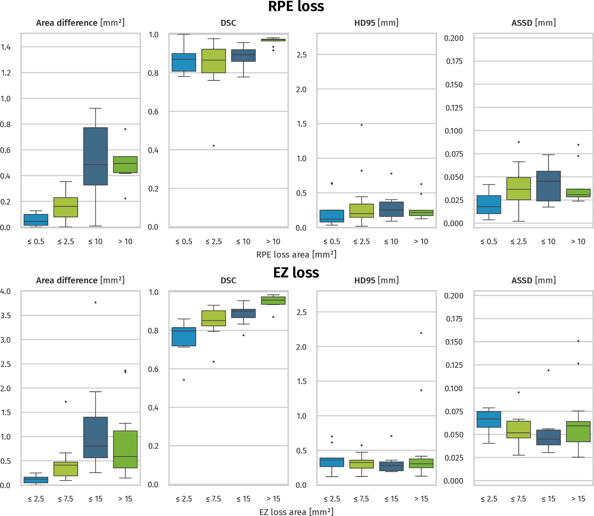
Performance metrics are summarized in Table ¿tbl:tab:performance95area95measurement?, with their distributions visualized via boxplots in Fig. 3. Detailed subset analyses of the stratified data are provided in the Supplemental Material (Table S1, Figure S1). Overall, the model achieved a mean DSC of 0.88 (95% CI: 0.84 to 0.90) for RPE loss and 0.87 (95% CI: 0.83 to 0.89) for EZ loss. Stratification by lesion size revealed the correlation between loss area and overall DSC; performance for RPE loss ranged from 0.84 for small lesions to 0.96 for large lesions, while EZ loss DSC ranged from 0.76 to 0.95.
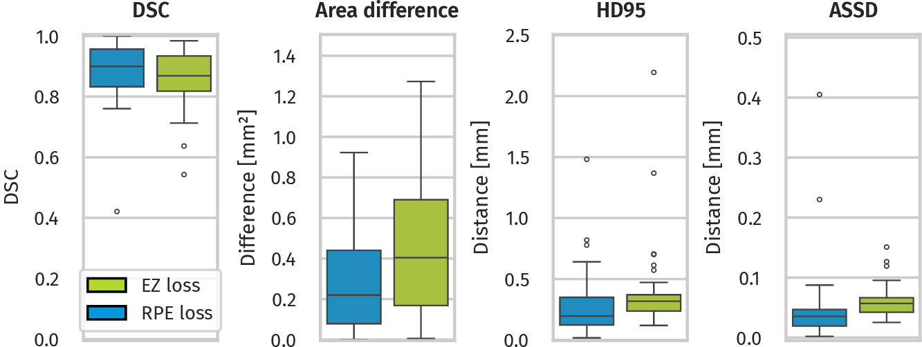
| Metric | RPE loss | EZ loss |
|---|---|---|
| Pearson’s r | 0.999 [0.998 to 1.000] | 0.996 [0.993 to 0.998] |
| DR Intercept [mm²] | 0.14 [0.047 to 0.28] | -0.56 [-0.93 to -0.27] |
| DR Slope[mm²] | 1.03 [1.015 to 1.05] | 1.02 [0.99 to 1.05] |
| 2-3 | Mean [95% CI] ± std | median ± IQR | |
| 2-3 AD loss area [mm²] | 0.34 [0.24 to 0.50] ± 0.40 | 0.22 ± 0.36 | 0.63 [0.46 to 0.93] ± 0.76 | 0.40 ± 0.52 |
| PD loss area [%] | 14.24 [10.60 to 18.53] ± 13.31 | 10.18 ± 15.54 | 8.57 [6.46 to 11.87] ± 8.73 | 6.39 ± 7.35 |
| DSC | 0.88 [0.84 to 0.90] ± 0.10 | 0.90 ± 0.12 | 0.87 [0.83 to 0.89] ± 0.10 | 0.87 ± 0.12 |
| Sensitivity | 0.92 [0.87 to 0.95] ± 0.12 | 0.96 ± 0.06 | 0.84 [0.80 to 0.87] ± 0.12 | 0.87 ± 0.17 |
| Specificity | 0.98 [0.97 to 0.99] ± 0.03 | 0.99 ± 0.02 | 0.96 [0.93 to 0.97] ± 0.07 | 0.98 ± 0.03 |
| Precision | 0.84 [0.81 to 0.88] ± 0.10 | 0.87 ± 0.15 | 0.90 [0.87 to 0.92] ± 0.08 | 0.92 ± 0.08 |
| NPV | 0.99 [0.99 to 1.00] ± 0.01 | 1.00 ± 0.01 | 0.94 [0.92 to 0.96] ± 0.06 | 0.97 ± 0.06 |
| HD95 [mm] | 0.29 [0.23 to 0.41] ± 0.27 | 0.20 ± 0.23 | 0.39 [0.32 to 0.56] ± 0.35 | 0.32 ± 0.13 |
| ASSD [mm] | 0.05 [0.04 to 0.08] ± 0.07 | 0.04 ± 0.03 | 0.06 [0.05 to 0.07] ± 0.03 | 0.06 ± 0.02 |
AD, PD, DR, AD, PD, DSC, NPV, HD95, ASSD
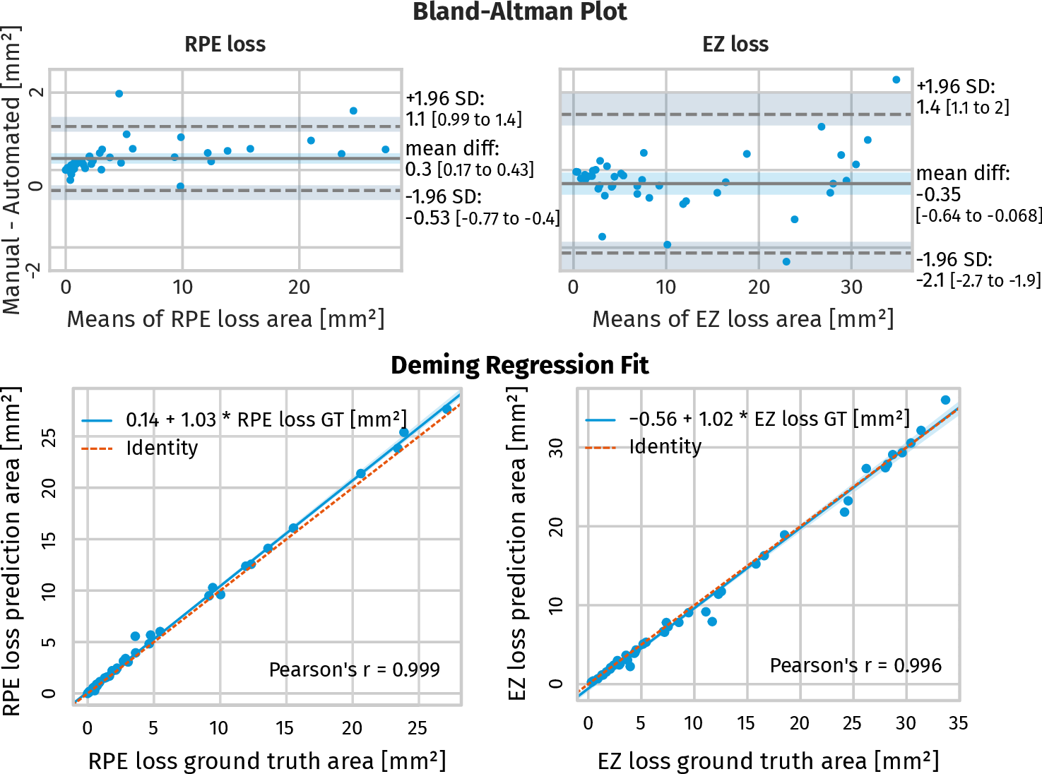
Area measurements demonstrated high correlation between manual and automated segmentations, with Pearson’s r of 0.999 (95% CI: 0.998 to 1.0) for RPE loss and 0.996 (95% CI: 0.993 to 0.998) for EZ loss. Deming regression parameters and Bland-Altman analysis (Fig. 4) indicated a slight systematic bias: a marginal over-segmentation of the RPE loss area (mean difference: 0.3 mm2 (95% CI: 0.17 to 0.43)) and a marginal under-segmentation of the EZ loss area (mean difference: -0.35 mm2 (95% CI: -0.64 to -0.068)).
3.0.0.3 Accuracy of layer segmentation and EZ thickness measurement:
As summarized in Table ¿tbl:tab:performance95layer95position?, the mean differences between manual and predicted positions for the IB-EZ, OB-OPR, and total EZ thickness were 3.33 μm, 5.17 μm, and 2.15 μm, respectively. Given a pixel spacing of 3.9 μm, the average deviations for both IB-EZ position and EZ thickness are less than a single pixel, demonstrating high accuracy in an OCT setting.
| Metric | Mean [95% CI] ± std | median ± IQR |
|---|---|
| AD IB-EZ layer position [μm] | 3.33 [3.08 to 3.83] ± 1.09 | 3.04 ± 0.94 |
| AD OB-OPR layer position [μm] | 5.17 [4.58 to 6.48] ± 2.60 | 4.46 ± 1.92 |
| AD IB-EZ to OB-OPR thickness [μm] | 2.15 [1.76 to 2.58] ± 1.37 | 2.00 ± 1.94 |
| PD IB-EZ to OB-OPR thickness [%] | 7.42 [6.17 to 8.73] ± 4.34 | 6.94 ± 7.29 |
| DSC IB-EZ to OB-OPR | 0.86 [0.77 to 0.90] ± 0.18 | 0.92 ± 0.10 |
AD, PD, IB-EZ, OB-OPR, DSC
3.0.0.4 Inter-reader reliability:
Table ¿tbl:tab:interreader95reliability? presents the inter-reader reliability between the two annotation groups (AN1 and AN2). The ICC(2,1) values for RPE and EZ loss area measurements were 0.985 (95% CI: 0.948 to 0.994) and 0.984 (95% CI: 0.743 to 0.996), respectively. Bland-Altman analysis (Fig. 5) and Deming regression intercepts (Table ¿tbl:tab:interreader95reliability?, Supplemental Figure S2) revealed a systematic bias in EZ loss measurements, with AN2 consistently over-segmenting the area relative to AN1. For mean RPE and EZ loss lesion sizes of 3.65 mm2 and 10.91 mm2, the LoAs were -1.7 to 0.87 mm2 and -3.8 to 0.81 mm2, respectively. Notably, the automated segmentation showed closer alignment with AN1, the group responsible for the training dataset.

| ICC(2,1) | Pearsons R | DR Intercept | DR Slope | ||
|---|---|---|---|---|---|
| RPE loss | AN2 vs AN1 | 0.985 [ 0.948 to 0.994 ] | 0.990 | 0.3 [0.06 to 0.51] | 1.0 [0.97 to 1.16] |
| AN1 vs automated | 0.993 [0.975 to 0.997] | 0.996 | 0.16 [0.045 to 0.34] | 1.04 [1.012 to 1.08] | |
| AN2 vs automated | 0.985 [0.966 to 0.993] | 0.984 | -0.14 [-0.36 to 0.11] | 1.00 [0.89 to 1.09] | |
| EZ loss | AN2 vs AN1 | 0.984 [ 0.743 to 0.996] | 0.994 | 1.2 [0.60 to 1.8] | 1.0 [0.98 to 1.1] |
| AN1 vs automated | 0.993 [0.985 to 0.997] | 0.994 | -0.8 [-1.38 to -0.29] | 1.0 [0.97 to 1.07] | |
| AN2 vs automated | 0.978 [0.493 to 0.995] | 0.994 | -2.1 [-2.80 to -1.2] | 1.0 [0.93 to 1.1] |
ICC, DR
3.0.0.5 Reproducibility:
The comparison of automated segmentations between screening and baseline visits from the OAKS and DERBY trials is summarized in Table ¿tbl:tab:reproducibility?. Reproducibility was excellent, with ICC(2,1) values of 0.995 (95% CI: 0.991 to 0.997) for RPE loss and 0.988 (95% CI: 0.978 to 0.993) for EZ loss. Deming regression and Bland-Altman analysis (Fig. 6) showed no significant bias relative to lesion size. The mean percentage difference in lesion area between the two visits was 3.33% for RPE loss and 3.58% for EZ loss, demonstrating high reproducibility of the automated measurements.

| RPE loss | EZ loss | |
|---|---|---|
| Mean ± std | median ± IQR | ||
| 2-3 Area at baseline [mm2] | 7.764 ± 3.389 | 7.543 ± 5.190 | 13.472 ± 6.228 | 11.874 ± 7.721 |
| AD loss area [mm2] | 0.251 ± 0.222 | 0.160 ± 0.268 | 0.643± 0.718 | 0.468 ± 0.746 |
| PD loss area [mm2] | 3.33 ± 2.97 | 2.97 ± 2.72 | 3.58 ± 0.82 | 3.45 ± 1.08 |
| ICC(2,1) | 0.995 [0.991 to 0.997] | 0.988 [0.978 to 0.993] |
| Pearson’s R | 0.996 [0.994 to 0.998] | 0.990 [0.984 to 0.994] |
| DR Intercept | 0.14 [-0.022 to 0.32] | 0.28 [-0.14 to 0.79] |
| DR Slope | 0.97 [0.943 to 0.99] | 0.96 [0.91 to 1.00] |
AD, PD, ICC, DR, IQR
3.0.0.6 B-scan density:
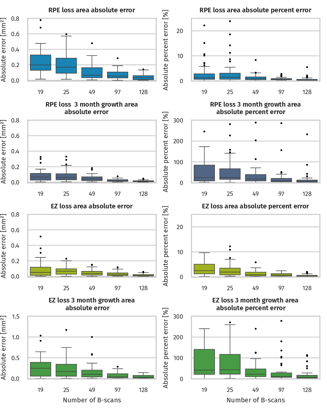
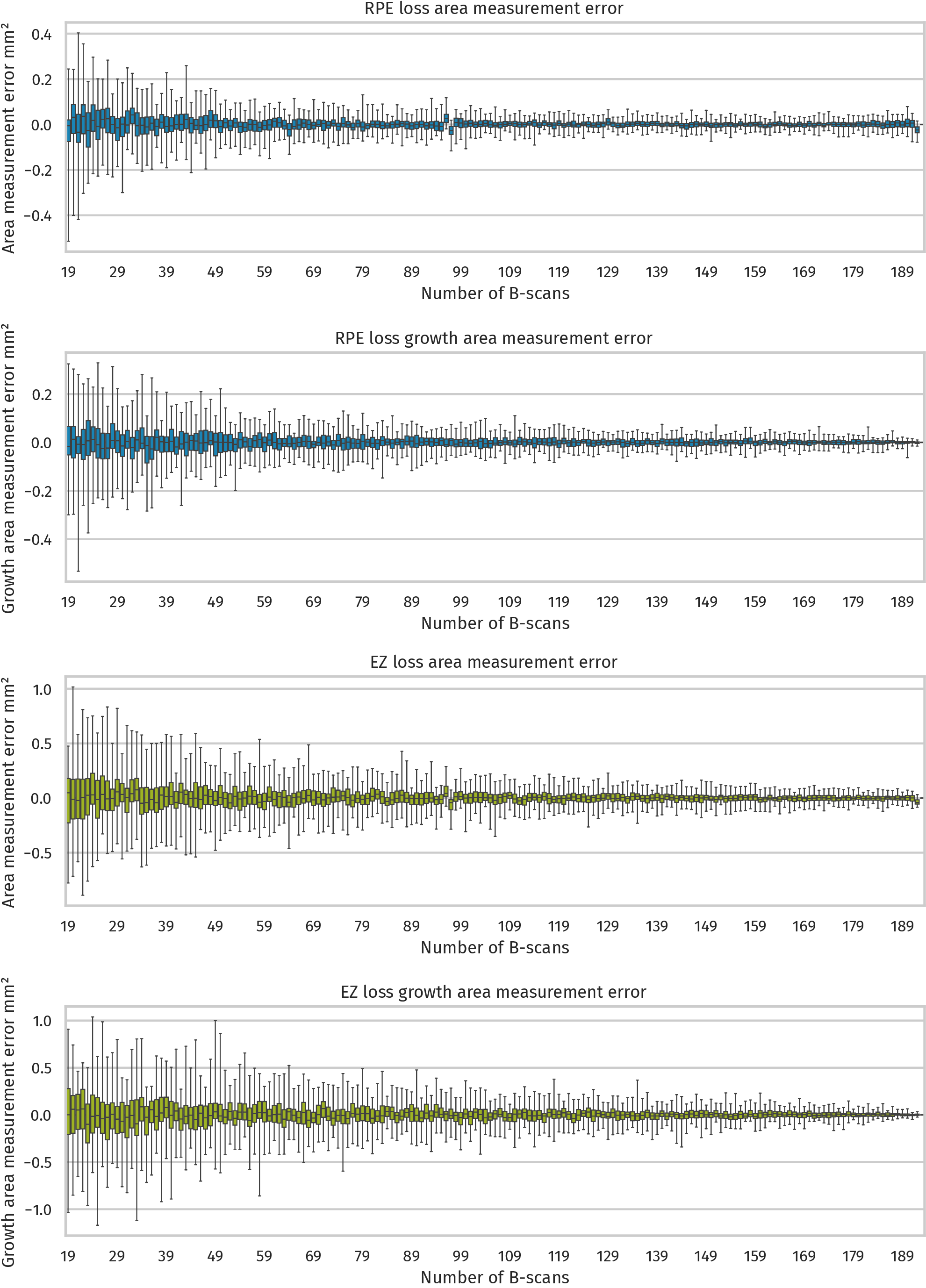
Table ¿tbl:tab:bscan95density? reports the MAE and MAPE for RPE loss, EZ loss, and their progression areas across standard B-scan patterns: 19, 25, 49, and 97 (Spectralis scanners) and 128 (Zeiss Cirrus and Topcon Maestro2 scanners), compared to a 193 B-scan baseline. Corresponding B-scan spacings were 314, 239, 122, 61, 47, and 31 μm . Error distributions are shown in Fig. 7, and Supplemental Figure S3 lists errors for all B-scan spacings from 19 to 192.
| GT loss area[mm²] (n=61) | GT 3 month progression absolute loss area [mm²] (n=45) | |||
| RPE loss | 5.38 ± 4.23 | 4.02 ± 7.24 | 0.32 ± 0.29 | 0.19 ± 0.40 | ||
| EZ loss | 10.08 ± 5.93 | 8.91 ± 9.71 | 0.61 ± 0.55 | 0.51 ± 0.70 | ||
| # B-scans | MAE loss area [mm²] | MAPE loss area [%] | MAE progression loss area [mm²] |
MAPE progression loss area [%] |
| RPE loss | ||||
| 19 | 0.08 [0.06 to 0.11] ± 0.10 | 2.52 [1.77 to 3.88] ± 3.83 | 0.08 [0.06 to 0.11] ± 0.07 | 106.71 [58.29 to 193.06] ± 228.82 |
| 25 | 0.07 [0.06 to 0.09] ± 0.06 | 2.81 [2.01 to 4.37] ± 4.32 | 0.08 [0.06 to 0.11] ± 0.08 | 95.80 [52.11 to 176.62] ± 200.22 |
| 49 | 0.04 [0.04 to 0.05] ± 0.04 | 1.20 [0.95 to 1.68] ± 1.28 | 0.05 [0.04 to 0.07] ± 0.04 | 93.16 [40.22 to 243.58] ± 288.92 |
| 97 | 0.03 [0.03 to 0.04] ± 0.03 | 0.78 [0.66 to 0.93] ± 0.55 | 0.02 [0.02 to 0.03] ± 0.02 | 29.66 [16.43 to 64.46] ± 68.65 |
| 128 | 0.02 [0.01 to 0.02] ± 0.01 | 0.54 [0.41 to 0.82] ± 0.80 | 0.01 [0.01 to 0.02] ± 0.01 | 23.09 [9.78 to 53.13] ± 66.48 |
| EZ loss | ||||
| 19 | 0.24 [0.20 to 0.28] ± 0.16 | 3.21 [2.61 to 3.91] ± 2.53 | 0.28 [0.21 to 0.35] ± 0.24 | 222.97 [126.79 to 395.48] ± 438.00 |
| 25 | 0.21 [0.17 to 0.24] ± 0.15 | 2.68 [2.19 to 3.45] ± 2.50 | 0.25 [0.19 to 0.33] ± 0.25 | 93.13 [63.21 to 145.06] ± 130.72 |
| 49 | 0.10 [0.08 to 0.13] ± 0.10 | 1.27 [1.00 to 1.56] ± 1.11 | 0.15 [0.11 to 0.22] ± 0.18 | 88.60 [52.12 to 152.89] ± 163.84 |
| 97 | 0.07 [0.06 to 0.09] ± 0.06 | 0.83 [0.69 to 0.99] ± 0.63 | 0.07 [0.05 to 0.09] ± 0.07 | 32.14 [20.59 to 56.67] ± 53.34 |
| 128 | 0.04 [0.03 to 0.05] ± 0.03 | 0.50 [0.38 to 0.63] ± 0.53 | 0.05 [0.04 to 0.06] ± 0.04 | 20.05 [12.77 to 31.50] ± 31.28 |
MAE, MAPE, GT
GA lesion progression was slow during the 3-month interval, making the progression area small relative to overall lesion size (e.g., 0.32 vs. 5.38 mm2 for RPE). Combined with large B-scan spacings, this resulted in high percentage errors, such as a 95% error for RPE loss progression using 25 B-scans (a 100% error equates to a factor-of-two overestimation). The primary cause of these errors is that the physical lesion progression is smaller than the spacing between slices, rendering the changes unobservable.
4 Discussion↩︎
Based on the work performed in the described path, we are able to present a deep learning-based algorithm for high-quality, high accuracy and fully automated segmentation of pivotal GA features in conventional retinal OCT images applicable to real-world settings and spanning a wide range of morphological conditions. The focus of our work are the two hallmark features relevant for GA monitoring in clinical trials and routine, i.e. RPE loss and outer photoreceptor degeneration (represented by EZ thinning and loss). We evaluated the accuracy of automated area and thickness measurements, as well as the precision of the segmentations in patients with a large range of GA manifestations secondary to AMD. Overall, we report high agreement between GT and automated segmentations, with a mean DSC of 0.88 and 0.87, and a Pearson’s r of 0.999 and 0.996 for RPE and EZ loss area, respectively.
4.0.0.1 Accuracy of RPE and EZ loss segmentation and measurements:
Area measurements demonstrated strong correlation between automated and manual segmentations. For very large lesions (\(> 20\) mm2), the algorithm tends to report slightly higher values, a trend visualized in the Deming regression and Bland-Altman plots. The high specificity (RPE loss: 0.98, EZ loss: 0.96) indicates that non-atrophic areas were rarely misclassified as atrophic. A high sensitivity and slightly lower precision for RPE loss (0.92 and 0.84, respectively) suggests a small trend towards over-segmentation. Qualitative analysis revealed that such "false positives" typically occur at irregular lesion borders or in regions showing early signs of atrophy that have not yet met the strict reader criteria for "complete" RPE loss, but which already manifest signs of atrophy. For a clinical assessment of RPE integrity, the borders are biologically not as distinct as jumping from completely healthy to completely lost RPE. In EZ segmentation sensitivity is marginally lower than precision (0.84 and 0.90), indicating a trend to slightly under-segment EZ loss compared to GT. As the EZ layer is primarily a thin and less reflective band, remaining EZ fragments at the zone of highest disease activity and cellular debris are expected. Both findings highlight the limitations of advanced image analysis technology by biology and visualization.
4.0.0.2 Subgroup analysis of RPE and EZ loss:
Training and validation datasets frequently exclude very small or very large lesions, potentially introducing selection bias. [@monesRateProgressionGeographic2018]. To reduce this risk, we included real-world data covering the full spectrum of GA progression, from early-stage to advanced lesions. Our stratified analysis further underscores an important limitation of DSC and other confusion-matrix–based metrics, including sensitivity and specificity, as these measures are strongly influenced by lesion size [@seghierImageSegmentationEvaluation2024]. For small lesions (\(\leq 0.5\)mm2), even minor boundary errors can disproportionately affect performance estimates relative to larger lesions. When considering common clinical trial size restrictions (2.5 to 17.5 mm2 in FILLY, OAKS and DERBY), our DSC increased to \(0.91 \pm 0.06\) for RPE loss and \(0.93 \pm 0.03\) for EZ loss. In contrast, surface distance metrics such as HD95 and ASSD proved more robust to size variations. We found that 95% of all automated segmentation surface points were within \(0.29 \pm 0.27\) mm (RPE) and \(0.39 \pm 0.13\) mm (EZ) of the manual annotations. HD95 and ASSD in subgroups stayed in the same range, independent on lesion size. The detection of small lesions is clinically relevant, as the biology of growth differs from larger ones [@coulibalyProgressionDynamicsEarly2023a].
4.0.0.3 Comparison with State-of-the-art:
Despite the sensitivity of metrics to lesion size, our results compare favourably to current methods. For RPE loss, our DSC of 0.88 is entirely consistent with Lachinov et al. [@lachinovProjectiveSkipConnectionsSegmentation2021] (0.92), al-Khersan et al.[@al-khersanDeepLearningBasedSegmentation2025] (0.82), Spaide et al. [@spaideEstimatingUncertaintyGeographic2025] (0.90), and the method by Morano et al. [@moranoDeepMultimodalFusion2024] (0.89) upon which our segmentation method is based. Yoshida et al. [@yoshidaDeepLearningApproaches2025] report a Pearson \(R^2\) of \(0.91\) (our method: \(0.998\)).
For EZ loss, our DSC of 0.87 outperforms Pfau et al. [@pfauProgressionPhotoreceptorDegeneration2020] (0.82), and our layer position MAE of \(3.33 \pm 1.09\) μm is even lower than the \(3.92 \pm 3.72\) μm reported by Mishra et al. [@mishraAutomatedRetinalLayer2020]. Riedl et al. [@riedlEffectPegcetacoplanTreatment2022] report a mean DSC of \(0.838 \pm 0.084\) for automatic segmentation of the EZ to OB-OPR region. In comparison, we report a mean DSC of \(0.86 \pm 0.18\). However, comparison with other methods is limited due to different datasets evaluated and different annotation criteria used.
Precise and reliable determination of EZ boundaries is critical. Although complete EZ loss is often considered a point of morphological no-return, microperimetry demonstrates that retinal sensitivity in these areas ranges between 8 and 10 dB, indicating substantial residual activity of "invisible" photoreceptors [@birnerStructureFunctionCorrelationDeepLearning2025; @ansariEvaluatingProgressionRetinal2025a]. Structure-function analyses indicate that EZ attenuation is a continuous rather than binary process; for instance, partial EZ loss represents a pathway of slowly progressive thinning [@kalraAutomatedIdentificationSegmentation2023]. Clinically, baseline EZ thinning is a major risk factor for both the conversion from iAMD to GA [@voglSpatiotemporalAlterationsRetinal2021a] and the subsequent progression rate of manifest lesions [@voglPredictingTopographicDisease2023]. Localized EZ thickness accurately predicts the risk of conversion at specific topographical points along the GA margin [@schmidt-erfurthLongitudinalAssessmentProgressive2025]. Furthermore, the ratio between EZ loss area and RPE loss area has been shown as an predictor for future GA progression rate [@maiDynamicsEZRPE2025]. However, the reported quartiles of ratios based on the OAKS & DERBY study eyes are slightly higher using this segmentation algorithm (compare Tables from [@maiDynamicsEZRPE2025] with Supplemental Table S2) due to higher sensitivity in detecting EZ loss. Crucially, EZ thickness serves as a strong structural predictor of retinal function, exhibiting a well-defined correlation with microperimetry sensitivity (µm/dB) [@birnerStructureFunctionCorrelationDeepLearning2025]. Moving forward, the integration of novel high-resolution imaging devices, such as the High-Resolution Spectralis [@frank-publigQuantificationsOuterRetinal2025], will further enhance the precision of EZ segmentation.
4.0.0.4 Inter-reader reliability:
The inter-reader study confirms that RPE loss can be annotated reliably across different groups (ICC 0.985), with the algorithm successfully reproducing these results. Reader-versus-algorithm ICC aligns closely with inter-reader ICC, indicating that the algorithm performs on par with human annotators while offering the advantage of perfectly consistent results. EZ segmentation remains more challenging [@leeChallengesAssociatedEllipsoid2021], requiring strict and detailed annotation protocols and expert training. Although inter-group agreement was high (ICC 0.984), we observed a slight bias: the second reader group (AN2) tended to classify "barely visible" EZ bands as loss, whereas the first group (AN1) classified them as present. Interestingly, the algorithm aligned more closely with AN1 for both loss types, who provided also the initial training data.
However, the reproducibility study validated that RPE loss and EZ loss can be segmented consistently, showing a high agreement between screening and baseline visits (ICC: 0.988; mean absolute percentage difference: 3.58%).
4.0.0.5 Effect of B-scan density on RPE and EZ loss measurement:
Evaluating various B-scan densities using simulated low-resolution segmentations revealed that larger lesions can be accurately measured even at lower densities (e.g., yielding only a 1.2% RPE loss error with a 49 B-scan pattern). However, GA progression is generally slow and highly variable locally, with an approximate progression rate of 1 mm per year [@voglPredictingTopographicDisease2023]. Consequently, progression across the B-scans may go unnoticed if the B-scan spacing is too large. Specifically, for the device used in this study, patterns of 97 to 128 B-scans provide the necessary resolution to accurately measure small lesions and reliably monitor the slow progression of GA, even over short follow-up intervals of 3 months.
4.0.0.6 Limitations:
A primary limitation is the axial resolution and B-scan density (49 slices) of the validation datasets. A single-slice discrepancy corresponds to an error of approximately 130 μm, which particularly impacts distance metrics at lesion borders. Additionally, slight misalignments in follow-up scans in the reproducibility study can affect the segmentation of focal EZ interruptions caused by SDDs. However, as these interruptions are small relative to the total GA area, they did not significantly impact the overall reproducibility scores.
4.0.0.7 Conclusion:
We have elaborated an accurate, fully automated, and reliable method for segmenting key GA features - RPE loss, EZ loss, and EZ thickness - in OCT images. By evaluating performance on real-world clinical data and incorporating inter-reader and reproducibility analyses, we have demonstrated that this algorithm is a robust tool for automated GA assessment in both research and clinical settings. The speed and reliability of a fully automated, high-precision algorithm eliminate the need for simultaneous manual oversight. This capability not only transforms the execution of clinical trials but also serves as a crucial prerequisite for the real-world management of GA. Furthermore, optimized EZ thickness assessments could alleviate the need for burdensome microperimetry, providing clinicians with a direct translation of structural data into functional insights for routine practice.
Disclosures↩︎
W-DV, HS, OL, AS and AW: RetInSight GmbH(E). USE: AbbVie(C), ADARx(C), Alcon(C), Alkeus(C), Apellis(C), Astellas(C), Aviceda(C), Bayer(C), Complement Therapeutics(C), Genentech(C), Kodiak(C), Medscape(C), Roche(C), Samsung(C), Topcon(C).
This study was supported by Apellis, a subsidiary of Biogen, Inc., Cambridge, MA, USA and RetInSight GmbH, Vienna, Austria.
4.0.0.8 Data availability.
Data underlying the results presented in this paper are not publicly available at this time but may be obtained from the authors upon reasonable request.
Abbreviations and Acronyms↩︎
2
Supplemental Content: Supplemental Figures↩︎

Supplemental Content: Supplemental Tables↩︎
| Stratification RPE loss area | \(\leq 0.5\) [mm²] | \(\leq 2.5\) [mm²] | \(\leq 10\) [mm²] | \(> 10\) [mm²] |
|---|---|---|---|---|
| Count | 9 | 15 | 10 | 9 |
| Metric | mean ± std | median ± IQR | |||
| AD loss area [mm²] | 0.06 ± 0.05 | 0.04 ± 0.09 | 0.17 ± 0.11 | 0.16 ± 0.15 | 0.61 ± 0.55 | 0.49 ± 0.45 | 0.60 ± 0.38 | 0.49 ± 0.13 |
| PD loss area [%] | 23.31 ± 12.22 | 23.09 ± 15.43 | 15.74 ± 12.73 | 16.31 ± 14.05 | 14.50 ± 15.59 | 9.50 ± 12.81 | 3.41 ± 1.47 | 3.63 ± 1.74 |
| Area Prediction [mm²] | 0.29 ± 0.23 | 0.18 ± 0.41 | 1.31 ± 0.73 | 1.15 ± 1.25 | 5.54 ± 2.54 | 5.20 ± 2.40 | 18.11 ± 6.55 | 16.08 ± 11.26 |
| Area GT [mm²] | 0.25 ± 0.19 | 0.15 ± 0.32 | 1.19 ± 0.62 | 0.93 ± 1.11 | 4.93 ± 2.47 | 4.13 ± 2.10 | 17.61 ± 6.22 | 15.53 ± 11.07 |
| DSC | 0.87 ± 0.07 | 0.87 ± 0.09 | 0.84 ± 0.14 | 0.87 ± 0.12 | 0.88 ± 0.06 | 0.89 ± 0.06 | 0.96 ± 0.02 | 0.97 ± 0.01 |
| HD95 [mm] | 0.23 ± 0.25 | 0.12 ± 0.17 | 0.33 ± 0.37 | 0.20 ± 0.19 | 0.29 ± 0.20 | 0.25 ± 0.21 | 0.27 ± 0.17 | 0.21 ± 0.08 |
| ASSD [mm] | 0.02 ± 0.01 | 0.02 ± 0.02 | 0.06 ± 0.10 | 0.04 ± 0.02 | 0.06 ± 0.06 | 0.05 ± 0.03 | 0.04 ± 0.02 | 0.03 ± 0.01 |
| Sensitivity | 0.93 ± 0.04 | 0.93 ± 0.05 | 0.88 ± 0.18 | 0.96 ± 0.14 | 0.94 ± 0.05 | 0.96 ± 0.03 | 0.97 ± 0.03 | 0.99 ± 0.01 |
| Specificity | 1.00 ± 0.00 | 1.00 ± 0.00 | 0.99 ± 0.00 | 0.99 ± 0.01 | 0.97 ± 0.02 | 0.98 ± 0.01 | 0.95 ± 0.04 | 0.96 ± 0.04 |
| Precision | 0.78 ± 0.10 | 0.77 ± 0.13 | 0.82 ± 0.09 | 0.81 ± 0.13 | 0.83 ± 0.09 | 0.84 ± 0.08 | 0.95 ± 0.02 | 0.96 ± 0.03 |
| NPV | 1.00 ± 0.00 | 1.00 ± 0.00 | 1.00 ± 0.00 | 1.00 ± 0.00 | 0.99 ± 0.01 | 0.99 ± 0.00 | 0.98 ± 0.01 | 0.99 ± 0.02 |
| Stratification EZ loss area | \(\leq 2.5\) [mm²] | \(\leq 7.5\) [mm²] | \(\leq 15\) [mm²] | \(> 15\) [mm²] |
| Count | 9 | 14 | 7 | 13 |
| Metric | mean ± std | median ± IQR | |||
| AD loss area [mm²] | 0.11 ± 0.09 | 0.12 ± 0.12 | 0.45 ± 0.41 | 0.41 ± 0.28 | 1.25 ± 1.23 | 0.80 ± 0.84 | 0.84 ± 0.74 | 0.59 ± 0.76 |
| PD loss area [%] | 10.69 ± 7.68 | 9.60 ± 7.47 | 10.75 ± 10.67 | 8.58 ± 8.16 | 11.31 ± 10.30 | 7.15 ± 7.55 | 3.27 ± 2.69 | 2.24 ± 2.91 |
| Area Prediction [mm²] | 1.29 ± 0.75 | 1.16 ± 1.23 | 4.33 ± 1.74 | 3.95 ± 2.25 | 9.19 ± 1.76 | 9.05 ± 2.41 | 25.78 ± 6.27 | 27.42 ± 7.52 |
| Area Groundtruth [mm²] | 1.40 ± 0.74 | 1.40 ± 1.17 | 4.67 ± 1.59 | 4.37 ± 1.79 | 10.44 ± 1.95 | 11.09 ± 2.98 | 25.83 ± 5.70 | 28.01 ± 5.44 |
| DSC | 0.76 ± 0.10 | 0.80 ± 0.10 | 0.85 ± 0.08 | 0.85 ± 0.08 | 0.88 ± 0.06 | 0.90 ± 0.04 | 0.95 ± 0.03 | 0.96 ± 0.04 |
| HD95 [mm] | 0.37 ± 0.19 | 0.36 ± 0.13 | 0.31 ± 0.12 | 0.32 ± 0.11 | 0.32 ± 0.18 | 0.28 ± 0.13 | 0.51 ± 0.59 | 0.30 ± 0.13 |
| ASSD [mm] | 0.06 ± 0.01 | 0.07 ± 0.02 | 0.05 ± 0.02 | 0.05 ± 0.02 | 0.05 ± 0.03 | 0.04 ± 0.02 | 0.06 ± 0.04 | 0.06 ± 0.02 |
| Sensitivity | 0.72 ± 0.10 | 0.74 ± 0.12 | 0.81 ± 0.11 | 0.83 ± 0.12 | 0.84 ± 0.10 | 0.88 ± 0.07 | 0.95 ± 0.03 | 0.97 ± 0.05 |
| Specificity | 0.99 ± 0.01 | 0.99 ± 0.01 | 0.98 ± 0.01 | 0.99 ± 0.01 | 0.98 ± 0.01 | 0.98 ± 0.01 | 0.89 ± 0.09 | 0.93 ± 0.11 |
| Precision | 0.81 ± 0.10 | 0.81 ± 0.13 | 0.89 ± 0.05 | 0.90 ± 0.06 | 0.94 ± 0.02 | 0.94 ± 0.03 | 0.95 ± 0.04 | 0.97 ± 0.04 |
| NPV | 0.99 ± 0.01 | 0.99 ± 0.01 | 0.97 ± 0.01 | 0.97 ± 0.02 | 0.93 ± 0.04 | 0.96 ± 0.05 | 0.89 ± 0.07 | 0.89 ± 0.06 |
AD, PD, DR, GT, AD, PD, DSC, NPV, HD95, ASSD
| Total number of scans | Scans used for analysis | EZ loss / RPE loss ratio quartiles |
|---|---|---|
| 904 | 897 | Q1 \(< 1.37\); Q2 \(\geq 1.37\) to \(< 1.67\); Q3 \(\geq 1.67\) to \(< 2.17\); Q4 \(\geq 2.1\) |