Maximizing Parallel Execution of Series-Parallel Task Graphs for Safety-Critical Embedded Control
June 30, 2026
Abstract
Safety-critical embedded control programs must complete each control cycle within a bounded period. Sequential execution on conventional processors can become a bottleneck when the dependency structure of the program contains subtasks that could be executed concurrently. This paper studies the Maximum Parallel Execution (MPE) problem for series-parallel task graphs under a staged batching model: compatible tasks inside one batch execute in parallel, while the selected batches are launched sequentially in a topological order that preserves precedence. We formulate MPE as a weighted clique-partitioning problem that minimizes the sum of batch execution times, with each batch cost determined by its slowest task. To solve this problem efficiently, we propose a Lagrangian-based Iterative Heuristic (LIH). LIH constructs a pricing-filtered restricted pool of feasible candidate batches from singleton columns and random greedy clique generation. It then applies Lagrangian pricing to guide column selection and uses a repair procedure to recover a legal clique partition. Experiments against a weighted mixed-graph-coloring branch-and-bound baseline and a randomized greedy baseline show that LIH matches the exact optimum in \(91.25\%\) of comparable instances, with an average gap of \(0.073\%\) and an average runtime of \(18.19\) ms. In the largest exact-reference node setting, the exact baseline requires hundreds of seconds on average, whereas LIH remains below \(50\) ms. We further present an end-to-end PLC ladder-logic case study in which PLCOpen-style programs are converted to MPE graphs, optimized by LIH, translated into FPGA-oriented HDL, and simulated against the original PLC scan execution.
Embedded control, FPGA acceleration, Lagrangian relaxation, maximum parallel execution, series-parallel graphs, task scheduling.
1 Introduction↩︎
A series-parallel (SP) task graph is a structured special case of a directed acyclic graph (DAG). It models a computation as subtasks composed by two fundamental operations: series composition, which chains subtasks that must execute sequentially due to data dependencies, and parallel composition, which groups independent subtasks that may execute concurrently. This recursive structure arises naturally in a broad class of safety-critical embedded control programs—PID regulation loops, sensor fusion pipelines, and fault-detection logic—where certain operations depend on the output of others while the remaining operations are mutually independent [1], [2]. Given such a task graph, a central question is: how should its subtasks be dispatched to maximize parallel execution and thereby minimize the overall completion time (makespan)? We refer to this as the Maximum Parallel Execution (MPE) problem on SP task graphs, and it is the subject of this paper.
The MPE problem is motivated by timing constraints in real-time embedded control. Safety-critical control systems—found in industrial automation, robotics, autonomous vehicles, and high-precision instrumentation, must complete their control algorithms within a bounded control period to guarantee stability and responsiveness [3], [4]. Traditionally, these control tasks are executed sequentially on microcontrollers or digital signal processors, and decades of effort have been devoted to optimizing serial performance through instruction-level pipelining, compiler optimizations, and clock-frequency scaling [5]–[7]. These serial techniques are increasingly constrained by power, frequency, and memory latency limits. At the same time, modern applications often demand shorter control periods, for example when faster physical dynamics or finer-grained actuation require a loop to run at millisecond or sub-millisecond scale. Exposing task-level parallelism is therefore an important way to reduce the time spent in one control cycle.
Field-Programmable Gate Arrays (FPGAs) are a natural platform for this form of parallelization. Prior implementations of industrial control, predictive current control, model predictive control, and IEC 61131-3 timer logic show that typical embedded control functions can be mapped to FPGA hardware with moderate resource usage and deterministic timing behavior [8]–[11]. Beyond their familiar role in neural-network acceleration [12], [13], FPGAs are attractive for embedded control because they combine hardware-level determinism, reconfigurability, low power consumption, and robustness in harsh operating environments [8], [14]. Under this resource-abundant setting, the main question is no longer processor allocation, but structure: which tasks can be batched together without violating dependencies, and in what staged order should those batches be executed?
Compared with scheduling on arbitrary DAGs, a well-studied but NP-hard problem in general [15], the SP restriction admits significantly more efficient solutions. SP graphs possess a recursive decomposition tree that mirrors their series-parallel construction, and this structure can be exploited algorithmically [1], [2], [16]. Yet, existing work on SP graph scheduling has largely focused on resource-constrained settings, such as limited processors, or general-purpose parallel platforms, and does not directly address the FPGA-oriented scenario where computation units are abundant but the goal is to maximize the parallelism exposed from an originally sequential program [2], [16]. Moreover, prior studies on FPGA-based control acceleration typically treat the task graph as a flat pipeline or rely on ad hoc manual partitioning, without systematically exploiting the SP structure inherent in control programs [5].
This paper formalizes the MPE problem on SP task graphs for FPGA platforms under the assumption of sufficient computation units, and proposes an efficient Lagrangian-based Iterative Heuristic (LIH) for generating static staged batching plans. Given a control program with an SP-like dependency structure, LIH exposes within-stage parallelism while preserving precedence consistency between stages.
The main contributions are as follows:
We formulate MPE on an augmented series-parallel task graph that combines precedence arcs, compatibility edges, weighted task costs, and staged batching semantics for FPGA-oriented execution.
We express MPE as a weighted clique-partitioning problem with contracted-graph acyclicity, giving both an exact column model and a direct interpretation in which each selected clique is one parallel hardware stage.
We propose LIH, which uses pricing-filtered candidate generation, Lagrangian reduced-cost pricing, feasibility repair, and local refinement to avoid enumerating the exponential space of feasible batches.
We evaluate LIH against an exact weighted mixed-graph-coloring baseline and a randomized greedy baseline, and further demonstrate the complete PLC ladder-to-HDL workflow through parsing, MPE optimization, Verilog generation, simulation, and scan-cycle comparison.
The remainder of this paper is organized as follows. Section 2 presents the system model and problem formulation. Section 3 describes the proposed Lagrangian-based iterative heuristic. Section 4 reports experimental results. Section 5 shows how a PLC ladder program is mapped to the MPE graph and how a batching plan can be realized on FPGA-oriented hardware. Related work is discussed in Section 6. Section 7 concludes the paper.
2 System Model and Problem Formulation↩︎
This section formulates Maximum Parallel Execution (MPE) as a clique-partitioning problem on an augmented series-parallel task graph (SPG). We first define the graph model and staged batching semantics, and then give the exact integer formulation used as the reference problem.
2.1 Series-Parallel Task Graph↩︎
An SPG describes a computation built from series and parallel composition. Series composition imposes an execution order, whereas parallel composition places subgraphs in the same logical region without an internal ordering relation. This structure appears naturally in embedded control programs, where serial data dependencies coexist with independent sensing, filtering, diagnosis, and actuation branches that can be mapped to parallel FPGA logic.
Let the input SPG be represented as a mixed graph6 \[G=(V,E,A),\] where \(V\) is the set of computational tasks, \(E\) is the set of undirected compatibility edges, and \(A\) is the set of directed precedence arcs. Each vertex \(v\in V\) represents an atomic operation, a function block, or a higher-level control action, and has a positive execution time \(w_v>0\). The directed graph \((V,A)\) is acyclic and follows the series-parallel precedence structure. A directed arc \((u,v)\in A\) means that task \(u\) must finish before task \(v\) can start. An undirected edge \(\{u,v\}\in E\) means that \(u\) and \(v\) are mutually compatible and may be placed in the same parallel execution batch.
The compatibility relation collects implementation conditions that cannot be represented by precedence alone, such as conflicting state updates, exclusive I/O access, or hardware resources that cannot be duplicated. Resource attributes such as LUT, DSP, BRAM, memory-port, or safety-partition usage can also be encoded in \(E\). In this paper we assume sufficient FPGA computation units for any selected batch, so the limiting factor is the dependency and compatibility structure of \(G\). Under this concurrent execution semantics, the duration of a selected batch is determined by its slowest task.
2.2 Clique Partitioning and Parallelization Semantics↩︎
Partitioning turns graph-level parallelism into an executable sequence of parallel batches. Write \(u\leadsto_A v\) if there is a directed path from \(u\) to \(v\) in \((V,A)\). A subset \(S\subseteq V\) is a feasible batch if its vertices are pairwise compatible and have no direct or transitive precedence relation: \[\{u,v\}\in E,\quad u\not\leadsto_A v,\quad v\not\leadsto_A u, \qquad \forall u,v\in S,\;u\neq v .\] Equivalently, \(S\) is a clique in the compatibility graph that does not collapse any precedence path. The execution cost of \(S\) is \[c(S)=\max_{v\in S} w_v .\] In the FPGA deployment, one batch corresponds to one execution stage: all tasks in \(S\) are enabled together, and inter-stage registers hold values required by later stages. Compared with serial execution, the local saving of a non-singleton batch is \(\sum_{v\in S}w_v-\max_{v\in S}w_v\). Singleton batches remain available for tasks that cannot be legally or profitably merged.
A clique partition \(\mathcal{C}=\{C_1,\ldots,C_m\}\) assigns every vertex to exactly one feasible batch: \[C_i\cap C_j=\emptyset\;(i\neq j), \qquad \bigcup_{i=1}^{m} C_i=V .\] We use staged sequential batching semantics. Tasks in the same batch execute concurrently, while batches are issued one at a time by a controller according to a topological order of the contracted graph. This preserves the sequential effects of the original program while exploiting spatial parallelism inside each stage.
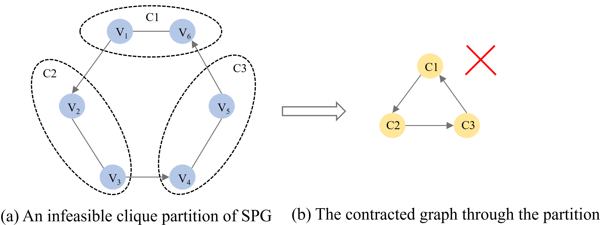
After each \(C_i\) is contracted into a super-vertex, every original arc \((u,v)\in A\) with \(u\in C_i\), \(v\in C_j\), and \(i\neq j\) induces an arc \(C_i\rightarrow C_j\). This contraction replaces several fine-grained tasks by one coarse-grained parallel stage. The partition is legal only if the contracted graph \(G/\mathcal{C}\) is acyclic, which ensures that the selected batches admit at least one staged execution order. Fig. 1 shows an infeasible partition whose contraction creates a directed cycle.
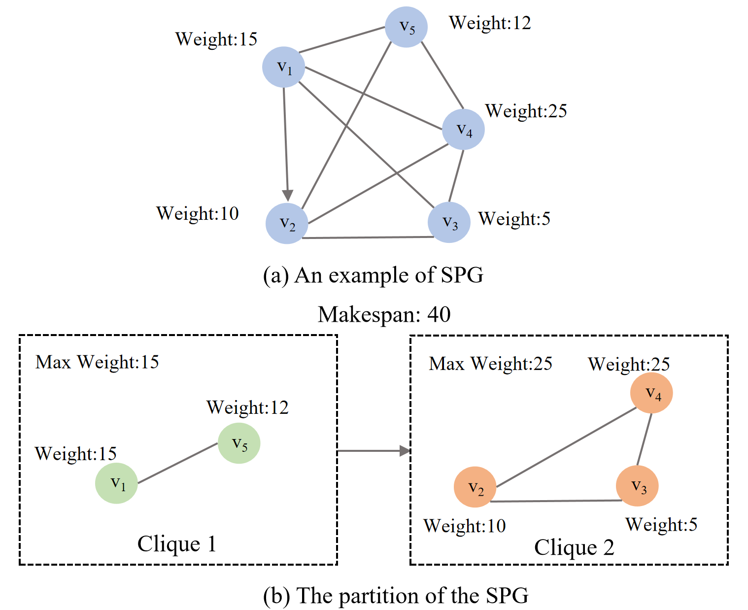
For a legal partition \(\mathcal{C}\), the makespan under the staged batching semantics is the sum of the selected batch costs: \[T(\mathcal{C}) = \sum_{C\in\mathcal{C}} c(C) = \sum_{C\in\mathcal{C}}\max_{v\in C}w_v . \label{eq:model-partition-cost}\tag{1}\] Thus, maximizing parallel execution is equivalent to minimizing the additive cost of legal batches. In Fig. 2, for example, the partition \(C_1=\{v_1,v_5\}\) and \(C_2=\{v_2,v_3,v_4\}\) has costs \(15\) and \(25\), giving \(T(\mathcal{C})=40\).
2.3 Maximum Parallel Execution Formulation↩︎
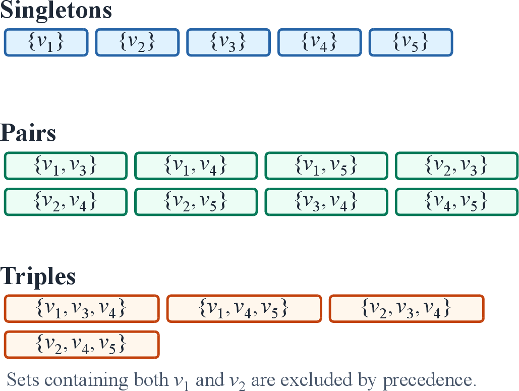
Let \(\mathcal{P}^{\star}\) be the unrestricted set of all feasible batches in \(G\). It contains every feasible clique satisfying compatibility and no-internal-path conditions. Fig. 3 illustrates \(\mathcal{P}^{\star}\) for the same SPG.
Each candidate batch is represented as a column \(p\in\mathcal{P}^{\star}\) with vertex set \(S_p\subseteq V\), cost \[c_p=\max_{v\in S_p}w_v ,\] and incidence coefficient \[a_{vp} = \begin{cases} 1, & \text{if } v\in S_p,\\ 0, & \text{otherwise}. \end{cases}\] The binary variable \(z_p\) indicates whether column \(p\) is selected: \[z_p = \begin{cases} 1, & \text{if } S_p \text{ is selected as a batch},\\ 0, & \text{otherwise}. \end{cases}\]
The Maximum Parallel Execution (MPE) problem is then formulated as \[\begin{align} T^{\star}(G)= \min_{z}\quad & \sum_{p\in\mathcal{P}^{\star}} c_p z_p \tag{2} \\ \text{s.t.}\quad & \sum_{p\in\mathcal{P}^{\star}} a_{vp}z_p = 1, && \forall v\in V, \tag{3} \\ & G/\{S_p:z_p=1\}\text{ is acyclic}, \tag{4} \\ & z_p\in\{0,1\}, && \forall p\in\mathcal{P}^{\star}. \notag \end{align}\] Constraint 3 is the exact coverage constraint: every task must be assigned to one and only one selected batch. Constraint 4 preserves global precedence consistency after batch contraction. The objective 2 minimizes the total execution time of the selected parallel batches.
2.4 Challenges for Parallelization↩︎
Although exact, the formulation is difficult to solve directly. It contains set-partitioning and clique-partitioning structure, which is NP-hard in general [15], and the column set \(\mathcal{P}^{\star}\) can be exponentially large. The selected columns must also cover every vertex exactly once and yield an acyclic contracted graph, so local clique feasibility alone is insufficient.
The next section therefore introduces a Lagrangian-based iterative heuristic. Instead of enumerating all of \(\mathcal{P}^{\star}\), it works with a restricted candidate set \(\mathcal{P}\subseteq\mathcal{P}^{\star}\) while retaining the same column notation \(S_p\), \(c_p\), \(a_{vp}\), and \(z_p\). The exact coverage equality 3 then becomes the source of the Lagrangian multipliers.
3 Lagrangian-based Iterative Heuristic↩︎
The exact model in Section 2 uses the unrestricted candidate set \(\mathcal{P}^{\star}\), which can be exponentially large. The Lagrangian-based Iterative Heuristic (LIH) instead works over a restricted pool \(\mathcal{P}\subseteq\mathcal{P}^{\star}\). Each column in \(\mathcal{P}\) is still a locally feasible clique; the restriction only limits which feasible cliques are considered.
LIH first builds a preliminary pool from singleton and random-greedy cliques. Because the useful cliques are unknown a priori, a warm-up Lagrangian pricing pass ranks the generated non-singleton columns. LIH keeps all singleton columns and only the top-ranked non-singleton columns for the main iterations, reducing the influence of low-value cliques while preserving a trivial feasible partition. The retained pool is then priced, repaired, and refined; repair is needed because the relaxed selection may overlap, miss vertices, or create a cycle after contraction.
For clarity, Table 1 lists the notation used in this section.
| Symbol | Meaning | Symbol | Meaning |
|---|---|---|---|
| \(G=(V,E,A)\) | SPG: tasks, compatibility edges, and precedence arcs. | \(\lambda_v\), \(\lambda\), \(\lambda_v^t\), \(\lambda^{\mathrm{w}}\) | Vertex multiplier, vector, iteration-\(t\) value, and warm-up vector. |
| \(u,v\) | Task vertices. | \(L(z,\lambda)\) | Lagrangian objective. |
| \(S\), \(S_p\) | Vertex subset; subset of column \(p\). | \(\bar{c}_p(\lambda)\), \(\bar{c}(\lambda)\) | Column reduced cost and vector. |
| \(w_v\), \(w\), \(w_{\max}\) | Vertex time, weight vector, maximum weight. | \(\phi(\lambda)\), \(\phi_t\) | Dual function and current dual value. |
| \(\mathcal{P}^{\star}\), \(\mathcal{P}\) | All feasible columns; restricted pool. | \(\mathcal{P}^{-}(\lambda)\), \(\mathcal{P}^{-}\) | Negative-reduced-cost columns. |
| \(\mathcal{P}_0\), \(\mathcal{P}_{\mathrm{sg}}\), \(\mathcal{P}_{\mathrm{rg}}\) | Preliminary, singleton, and random-greedy pools. | \(h_v(\lambda)\), \(h_v\) | Relaxed coverage count. |
| \(\eta\) | Fraction of non-singleton columns retained after warm-up pricing. | \(g_v(\lambda)\), \(g_v\), \(g^t\) | Coverage violation/subgradient. |
| \(p\), \(m_0\), \(m\), \(n\), \(q\) | Column index, preliminary columns, retained columns, vertices, and maximum column size. | \(\alpha_t\), \(\rho\), \(\epsilon\) | Step size, scale, and minimum step. |
| \(m_{\max}\), \(R_{\mathrm{rg}}\), \(\xi\), \(\Delta\) | Pool cap, random-greedy rounds, seed, and optional deadline. | \([x]_{\epsilon}^{w_{\max}}\), \(x\) | Scalar clipping to \([\epsilon,w_{\max}]\). |
| \(\ell\), \(V^{\downarrow}\), \(V_{\pi}\) | Random-greedy round, ordered list, and shuffled list. | \(M\), \(\Pi_{[-M,M]}\) | Multiplier bound and projection. |
| \(C\), \(\mathcal{C}\) | Clique/batch and clique partition. | \(UB_t\), \(UB\) | Best feasible objective value. |
| \(\mathcal{C}^{0}\), \(\widehat{\mathcal{C}}\), \(\mathcal{C}^{best}\) | Initial, repaired, and best partitions. | \(\mathrm{saving}(p)\), \(\tau(p)\), \(\mathrm{score}(p)\) | Repair saving, insertion order, and ranking key. |
| \(c(S)\), \(c(C)\), \(c_p\) | Batch or column cost. | \(t\), \(T\), \(h\) | Iteration index, limit, and repair interval. |
| \(a_{vp}\) | if \(v\in S_p\), 0 otherwise. | \(\|\cdot\|_2\), \(|\cdot|\), \(O(\cdot)\) | Norm, cardinality, complexity. |
| \(z_p\), \(z_p(\lambda)\) | Column selection and relaxed selection. | \(\emptyset\), \(\mathbb{R}\), \(\{0,1\}\) | Empty, real, and binary sets. |
| \(G/\{S_p:z_p=1\}\), \(G/\mathcal{C}\) | Contracted graph. |
Lagrangian relaxation moves coupling constraints into the objective with multipliers [17], [18]. In LIH, the multipliers act as vertex prices: over-covered vertices become more expensive, whereas uncovered vertices become cheaper. The pricing step therefore provides both a dual search signal and a ranking rule for candidate cliques.
3.1 Restricted Column Model and Relaxation↩︎
We reuse the notation introduced in Section 2. The only change from the exact formulation is the candidate set: \[\mathcal{P}\subseteq\mathcal{P}^{\star}, \qquad \{\{v\}:v\in V\}\subseteq\mathcal{P}.\] For each \(p\in\mathcal{P}\), the vertex set \(S_p\), cost \(c_p\), incidence coefficient \(a_{vp}\), and binary selection variable \(z_p\) have the same meaning as in Section 2. The preliminary pool can be written as \[\mathcal{P}_0 = \mathcal{P}_{\mathrm{sg}} \cup \mathcal{P}_{\mathrm{rg}},\] where \(\mathcal{P}_{\mathrm{sg}}\) contains singleton columns and \(\mathcal{P}_{\mathrm{rg}}\) contains random greedy cliques. LIH then applies a warm-up pricing screen to obtain the working pool \[\mathcal{P} = \mathcal{P}_{\mathrm{sg}} \cup \operatorname{Top}_{\eta} \bigl(\mathcal{P}_0\setminus\mathcal{P}_{\mathrm{sg}}\bigr),\] where \(\operatorname{Top}_{\eta}(\cdot)\) denotes the top \(\eta\) fraction of non-singleton columns under the warm-up reduced-cost ranking. The singleton columns ensure that the restricted model always has at least the serial feasible partition.
Using these columns, the restricted column-selection model is formulated as \[\begin{align} \min_{z}\quad & \sum_{p\in\mathcal{P}} c_p z_p \notag \\ \text{s.t.}\quad & \sum_{p\in\mathcal{P}} a_{vp}z_p = 1, && \forall v\in V, \tag{5} \\ & G/\{S_p:z_p=1\}\text{ is acyclic}, \tag{6} \\ & z_p\in\{0,1\}, && \forall p\in\mathcal{P}. \notag \end{align}\] Constraint 5 enforces exact coverage, and constraint 6 enforces acyclicity after contraction. Since \(\mathcal{P}\) is only a subset of \(\mathcal{P}^{\star}\), the restricted optimum may be worse than the unrestricted optimum; LIH accepts this trade-off to avoid the full exponential column space.
Relaxation Strategy
The local feasibility of each column is guaranteed during candidate generation: LIH checks pairwise compatibility and rejects cliques containing a directed precedence path. Coverage, however, is global. The equality \[\sum_{p\in\mathcal{P}} a_{vp}z_p=1\] couples all columns that contain vertex \(v\).
LIH therefore relaxes the exact coverage constraints and assigns one multiplier \(\lambda_v\) to each vertex. If the relaxed solution covers \(v\) more than once, \(\lambda_v\) is increased, making columns containing \(v\) more expensive. If the relaxed solution does not cover \(v\), \(\lambda_v\) is decreased, making columns containing \(v\) more attractive. Thus, the multipliers are adaptive vertex prices derived directly from 3 .
The pricing step is therefore a search guide rather than a complete feasibility mechanism: coverage and contracted acyclicity are restored later by repair, while the relaxed subproblem remains separable by columns.
3.2 Lagrangian Pricing and Multiplier Update↩︎
Let \(\lambda_v\in\mathbb{R}\) be the Lagrange multiplier associated with the coverage equality of vertex \(v\). For a fixed multiplier vector \[\lambda=(\lambda_v)_{v\in V},\] the Lagrangian objective is obtained by adding the weighted coverage violation to the original objective: \[\begin{align} L(z,\lambda) &= \sum_{p\in\mathcal{P}} c_p z_p + \sum_{v\in V}\lambda_v \left( \sum_{p\in\mathcal{P}}a_{vp}z_p - 1 \right) \notag \\ &= \sum_{p\in\mathcal{P}} c_p z_p + \sum_{v\in V} \sum_{p\in\mathcal{P}} \lambda_v a_{vp}z_p - \sum_{v\in V}\lambda_v . \label{eq:m7-lagrangian-split} \end{align}\tag{7}\]
Exchanging the summation order gives \[\begin{align} \sum_{v\in V} \sum_{p\in\mathcal{P}} \lambda_v a_{vp}z_p &= \sum_{p\in\mathcal{P}} \sum_{v\in V} \lambda_v a_{vp}z_p . \end{align}\] Since \(a_{vp}=1\) only when \(v\in S_p\), \[\begin{align} \sum_{v\in V} \lambda_v a_{vp}z_p &= \left( \sum_{v\in S_p}\lambda_v \right)z_p . \label{eq:m7-incidence-rewrite} \end{align}\tag{8}\] Substituting 8 into 7 gives \[\begin{align} L(z,\lambda) &= -\sum_{v\in V}\lambda_v + \sum_{p\in\mathcal{P}} \left( c_p+\sum_{v\in S_p}\lambda_v \right)z_p . \label{eq:m7-lagrangian-collected} \end{align}\tag{9}\]
Equation 9 defines the reduced cost of column \(p\): \[\bar{c}_p(\lambda) = c_p+\sum_{v\in S_p}\lambda_v . \label{eq:m7-reduced-cost}\tag{10}\]
For a fixed multiplier vector \(\lambda\), the relaxed pricing problem is \[\min_{z\in\{0,1\}^{|\mathcal{P}|}} L(z,\lambda).\] Because coverage and contracted acyclicity are relaxed during pricing, each \(z_p\) can be optimized independently: \[z_p(\lambda)= \begin{cases} 1, & \text{if } \bar{c}_p(\lambda)<0,\\ 0, & \text{if } \bar{c}_p(\lambda)\geq 0 . \end{cases} \label{eq:m7-relaxed-selection}\tag{11}\] Thus, only negative-reduced-cost columns are selected in the relaxed solution.
Substituting the best independent decisions from 11 into 9 yields the Lagrangian dual function \[\phi(\lambda) = -\sum_{v\in V}\lambda_v + \sum_{p\in\mathcal{P}} \min\{0,\bar{c}_p(\lambda)\}. \label{eq:m7-dual-function}\tag{12}\] LIH does not solve the dual problem to optimality. It uses \(\phi(\lambda)\) and the reduced costs as search signals: a small reduced cost indicates either a low clique cost, under-covered vertices, or both.
Subgradient Multiplier Update
The dual function 12 is piecewise linear and may be non-differentiable. Therefore, LIH updates the multipliers by a subgradient method.
Let \[\mathcal{P}^{-}(\lambda) = \{p\in\mathcal{P}:\bar{c}_p(\lambda)<0\}\] be the set of columns selected by the relaxed pricing rule. The coverage count of vertex \(v\) in this relaxed solution is \[h_v(\lambda) = \sum_{p\in\mathcal{P}^{-}(\lambda)} a_{vp}.\] The corresponding coverage violation is \[g_v(\lambda) = h_v(\lambda)-1 .\] This expression is inherited directly from the relaxed coverage equality \(\sum_{p\in\mathcal{P}}a_{vp}z_p-1=0\), so \(g_v(\lambda)\) is a valid subgradient component for multiplier \(\lambda_v\).
The multiplier update is \[\lambda_v^{t+1} = \Pi_{[-M,M]} \left( \lambda_v^t+\alpha_t g_v^t \right), \quad \forall v\in V,\] where \(\Pi_{[-M,M]}\) denotes projection onto the interval \([-M,M]\). In the implementation, \[M=2w_{\max}, \qquad w_{\max}=\max_{v\in V}w_v .\] The projection prevents excessively large multipliers from dominating the original clique costs and stabilizes the search.
The update follows the price interpretation: over-covered vertices \((h_v>1)\) become more expensive, uncovered vertices \((h_v=0)\) become cheaper, and exactly covered vertices keep the same price.
Let \(UB_t\) be the best feasible objective value found so far, and let \[\phi_t=\phi(\lambda^t).\] When \(\phi_t<UB_t\), LIH uses a Polyak-style step size: \[\alpha_t = \left[ \rho\frac{UB_t-\phi_t}{\|g^t\|_2^2} \right]_{\epsilon}^{w_{\max}}, \quad \text{if } \phi_t<UB_t, \label{eq:m7-polyak-step}\tag{13}\] where \(\rho>0\) is a step-scale parameter and \[[x]_{\epsilon}^{w_{\max}} = \min\{w_{\max},\max\{\epsilon,x\}\}.\] Here, \(\epsilon>0\) is a small minimum step-size parameter. It provides the lower clipping bound, so an active multiplier update is not reduced to an exactly zero step by the step-size rule.
The numerator \(UB_t-\phi_t\) measures the current primal-dual gap, while \(\|g^t\|_2^2\) normalizes the update by the coverage violation.
When \(\phi_t\geq UB_t\), LIH switches to a damped fallback step: \[\alpha_t = \left[ \rho \frac{w_{\max}}{\sqrt{t}\max\{1,\|g^t\|_2^2\}} \right]_{\epsilon}^{w_{\max}} . \label{eq:m7-damped-step}\tag{14}\] This fallback keeps the multiplier update active, while the factor \(1/\sqrt{t}\) gradually reduces oscillation in later iterations.
3.3 Candidate Pool, Repair, and Local Refinement↩︎
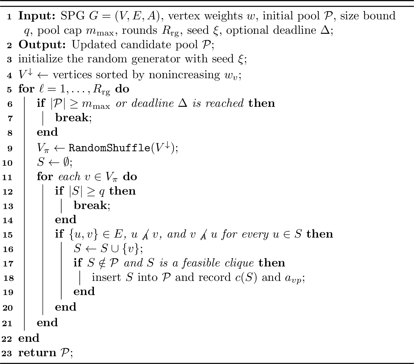
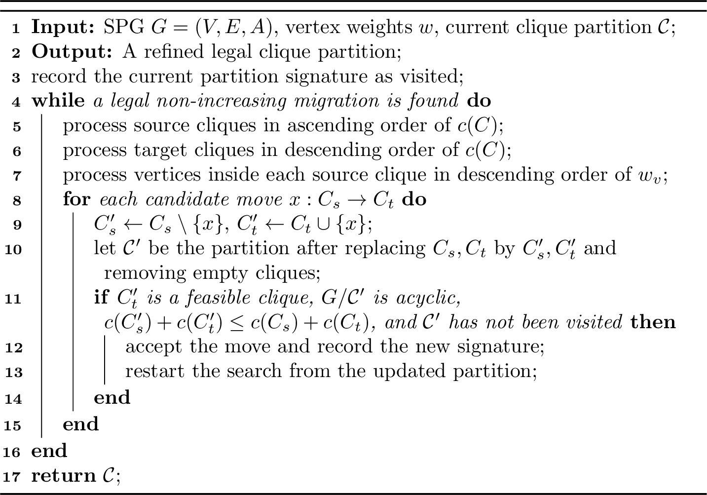
The candidate pool is constructed once before the main Lagrangian iterations. Singleton columns guarantee coverage and define the serial initial partition \(\mathcal{C}^0=\{\{v\}:v\in V\}\). Algorithm 4 adds locally feasible multi-vertex cliques by checking compatibility, precedence paths, size, duplicates, and the pool cap.
The resulting preliminary pool \(\mathcal{P}_0\) may still contain many low-value cliques. LIH therefore performs one warm-up pricing iteration and ranks non-singleton columns by \(\bar{c}_p(\lambda^{\mathrm{w}})/|S_p|\), where \(\lambda^{\mathrm{w}}\) is the warm-up multiplier vector. It then keeps all singletons and the top \(\eta\) fraction of non-singleton columns. In our experiments, \(\eta=5\%\) is sufficient to retain nearly all columns used by optimal partitions on exact-reference instances. The remaining task is to select disjoint retained columns whose contraction is acyclic.
Repairing the Relaxed Solution
The relaxed solution from 11 may overlap, miss vertices, or create a cycle after contraction. LIH therefore uses reduced costs only as guidance and repairs the selection into a legal partition.
Each candidate column \(p\) is assigned a repair score. Let \[\mathrm{saving}(p) = \sum_{v\in S_p}w_v-c_p .\] This value measures the local time saved by executing the vertices of \(S_p\) together instead of executing them as singleton batches. Let \(\tau(p)\) denote the insertion order of column \(p\) in the generated pool. The columns are sorted lexicographically by \[\mathrm{score}(p) = \left( \frac{\bar{c}_p(\lambda)}{|S_p|}, -\mathrm{saving}(p), -|S_p|, c_p, \tau(p) \right).\] The repair first prefers low reduced cost per vertex, then larger singleton savings, larger columns, lower execution cost, and earlier generated columns.
The repair scans this ranked list and accepts a column only if two conditions hold. First, all vertices in the column must still be uncovered. Second, adding the column to the already accepted columns, while leaving all remaining uncovered vertices as singleton columns, must keep the contracted directed graph acyclic. The second condition is a look-ahead feasibility test: it prevents the repair from accepting a locally attractive clique that would make the final partition impossible to schedule.
If no multi-vertex column can be accepted, LIH inserts the heaviest remaining vertex as a singleton, guaranteeing progress and feasibility. After exact coverage is obtained, LocalRefine tries non-increasing legal vertex migrations among
cliques while preserving clique feasibility and contracted acyclicity; repeated partition signatures are rejected to prevent cycling. Algorithm 5 summarizes the routine.
3.4 Complete Procedure, Complexity, and Limitations↩︎
Algorithm 6 summarizes LIH. The algorithm initializes the singleton partition, builds the pricing-filtered restricted pool, and then sets all main-loop multipliers to zero. Each iteration prices columns, periodically repairs and refines a feasible partition, and updates the multipliers from the coverage violation. The repair interval \(h\), step parameters \(\rho,\epsilon\), column-size bound \(q\), pool-generation parameters \(m_{\max},R_{\mathrm{rg}},\xi,\Delta\), and screening fraction \(\eta\) control the search.

Complexity and Limitations
We state the time bound in Lemma 1. Let \(n=|V|\), \(m_0=|\mathcal{P}_0|\) be the preliminary-pool size, \(m=|\mathcal{P}|\) be the retained working-pool size, \(m_d=|A|\), and let \(q\) be the maximum candidate-column size. The pricing screen gives \(m\le n+\lceil\eta(m_0-n)\rceil\). Let \(T\) be the number of Lagrangian iterations, \(h\) the repair interval, \(r_{\mathrm{rep}}=O(T/h)\) the number of repair calls, \(b\) the repair scan width, \(c\le n\) the number of cliques in the current partition, and \(L\) the number of local-refinement passes after one repair.
Lemma 1. Under the above notation, Algorithm 6 runs in \[\begin{align} O\bigl(&R_{\mathrm{rg}}nq +m_0(q^2+q+\log m_0) +T(mq+n)\\ &+r_{\mathrm{rep}}\bigl(mq\log m+nb(q+n+m_d)\\ &\qquad+Lc^2q(q+n+m_d)\bigr)\bigr). \end{align}\] Since \(c\le n\), the refinement term is \(O(Ln^2q(q+n+m_d))\) in the worst case.
Proof. Candidate generation scans \(R_{\mathrm{rg}}\) randomized vertex orders while growing cliques of size at most \(q\), and checking, recording, pricing, and ranking at most \(m_0\) columns gives \(O(R_{\mathrm{rg}}nq+m_0(q^2+q+\log m_0))\). Each Lagrangian iteration evaluates reduced costs and relaxed coverage counts over the retained pool, which costs \(O(mq+n)\). A repair call ranks retained columns, performs at most \(n\) insertions, and scans up to \(b\) candidates per insertion, giving \(O(mq\log m+nb(q+n+m_d))\). Local refinement checks source–target clique pairs and legal vertex moves for \(L\) passes, giving \(O(Lc^2q(q+n+m_d))\). Multiplying the repair and refinement costs by \(r_{\mathrm{rep}}\) yields the stated bound. ◻
The lemma shows the intended design trade-off: pricing over the bounded retained pool is polynomial and relatively cheap, while repair and refinement dominate because they repeatedly check contracted-graph feasibility.
The quality of LIH depends on the restricted candidate pool. If a useful clique is never generated or is removed by screening, the Lagrangian selection step cannot choose it. This is the central trade-off of the method: restricting \(\mathcal{P}\) greatly reduces the search complexity, while random greedy construction and the warm-up pricing screen aim to preserve the columns that are most valuable for parallel execution. Empirically, retaining all singleton columns and the top \(5\%\) of non-singleton columns provides a compact pool that is sufficient for near-optimal solutions in the tested instances.
4 Evaluation↩︎
This section evaluates MPE on randomly generated series-parallel task graphs. We compare solution quality and runtime under varying graph sizes, compatibility densities, precedence ratios, and task-weight distributions using three methods.
Weighted BB-MGC. An exact branch-and-bound baseline adapted from the mixed graph coloring framework in [19]. Because mixed graph coloring is equivalent to our clique-partitioning formulation after complementing the compatibility edge set, this method provides the optimal weighted makespan when it finishes within the time limit.
Randomized Greedy (RG). A randomized constructive baseline that repeatedly scans a randomized topological order and inserts each vertex into one feasible existing batch chosen from a small ranked candidate list.
LIH. The proposed Lagrangian-based Iterative Heuristic in Section 3 and Algorithm 6. LIH builds a preliminary candidate pool, retains all singleton columns and the top \(5\%\) of non-singleton columns after warm-up pricing, and then repairs the priced relaxed solution into a legal clique partition.
All methods are implemented in C++ and compiled with G++ 11.2 using the -O3 option. The experiments are run on a computer equipped with an AMD Ryzen 7 8745HS processor at 3.80 GHz and 32 GB RAM. Each run is terminated if it does not finish
within 1800 seconds.
4.1 Baselines and Experimental Setup↩︎
The weighted BB-MGC baseline uses the mixed graph coloring view. In MPE, \(E\) denotes compatibility, whereas in mixed graph coloring undirected edges denote conflicts. We therefore construct \[G^{c}=(V,\overline{E},A),\] where \(\overline{E}=\binom{V}{2}\setminus E\). A color class in \(G^{c}\) then corresponds to a compatible batch in the original MPE instance.
The branch-and-bound framework in [19] is unit-time; we keep its exact coloring search but replace the unit color-class cost by \(c(C)=\max_{v\in C}w_v\). The feasible coloring space is unchanged, so the adapted baseline remains exact for the weighted makespan in 1 ; pruning and incumbent comparisons are also evaluated with the weighted batch cost.
Randomized Greedy Baseline
Algorithm 7 gives the randomized greedy baseline. Each round processes vertices in a randomized topological order and inserts the current vertex into a feasible existing batch when possible. Candidate batches are ranked by incremental partition cost, new batch cost, and batch size; RG then samples uniformly from the best \(K\) candidates. The method remains purely constructive but can escape some unlucky early insertions.
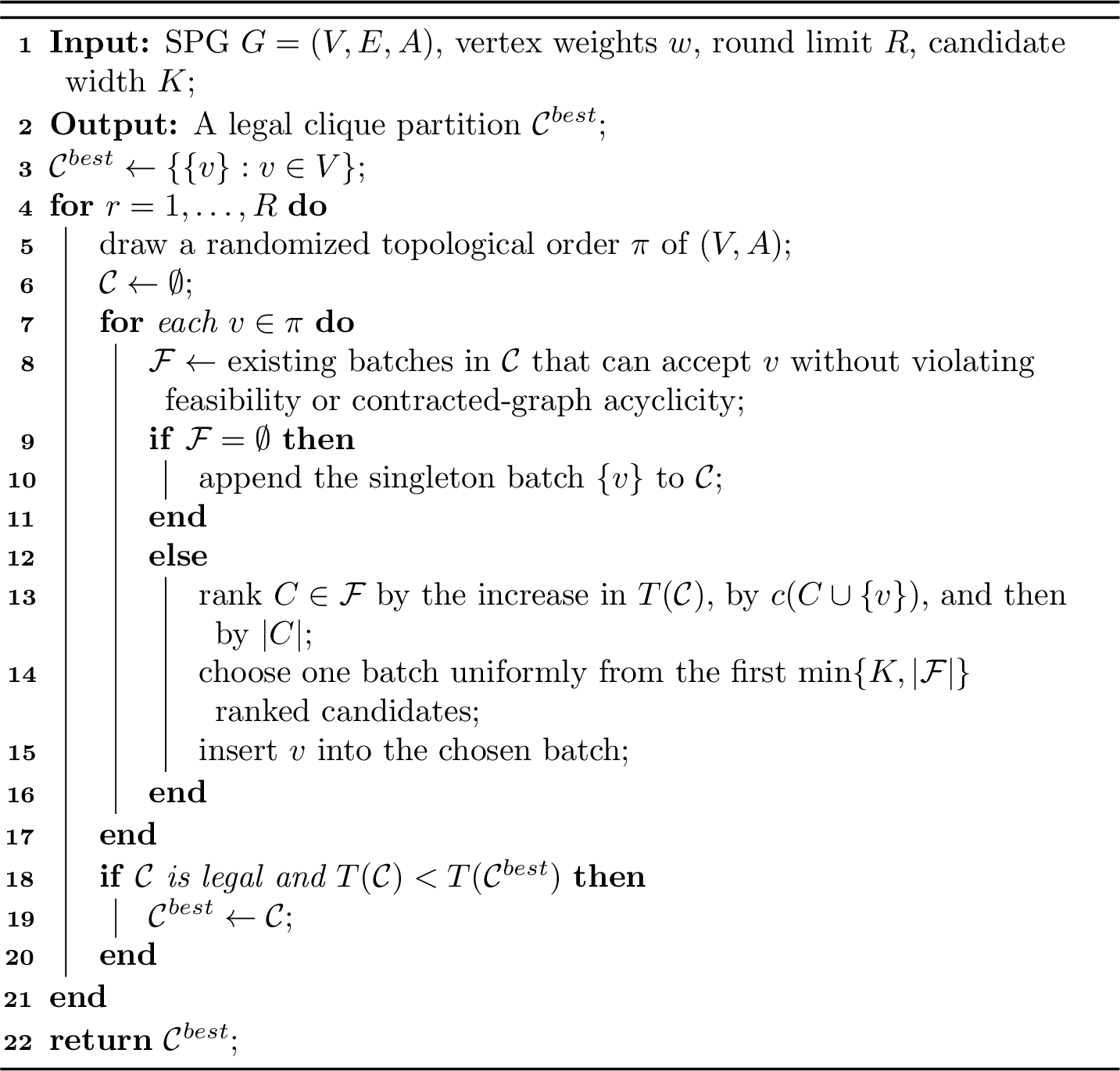
RG and LIH use the same feasibility checks and objective. RG relies on local insertions, whereas LIH uses Lagrangian prices to guide a repaired column selection.
Instance Generation
Synthetic SPG instances are generated in the mixed-graph form \(G=(V,E,A)\).
Vertices and weights. Each instance contains \(N_v\) vertices. By default, \(N_v=25\). Each vertex weight \(w_v\) is sampled from \([5,95]\). We test Uniform, Normal, and Bimodal distributions. The default setting is Normal with \(\mu=50\) and \(\sigma=15\). The Bimodal setting uses two modes with \(\mu_1=20\), \(\mu_2=80\), and \(\sigma=5\).
Compatibility and precedence. We first sample \(N_a=\lfloor D N_v(N_v-1)/2\rfloor\) unordered vertex pairs, where \(D\) is the graph density and defaults to \(30\%\). A fraction \(R\) of these pairs is converted into directed precedence arcs. The default value is \(R=5\%\). Directed arcs are oriented according to a random topological order to avoid directed cycles. The remaining unordered pairs are inserted into \(E\) as compatibility edges. Instances that violate the required acyclicity or SPG structure are regenerated.
Table 2 lists the defaults; each experiment group varies one parameter at a time.
| Parameter | Default value |
|---|---|
| Number of vertices \(N_v\) | 25 |
| Graph density \(D\) | \(30\%\) |
| Directed-edge ratio \(R\) | \(5\%\) |
| Weight range | \([5,95]\) |
| Weight distribution | Normal, \(\mu=50,\sigma=15\) |
| Instances per setting | 200 |
| Time limit | 1800 seconds |
| Group | Varied parameter | Candidate values |
|---|---|---|
| G1 | Number of vertices \(N_v\) | \(5,10,15,20,25,30,35\) |
| G2 | Graph density \(D\) | \(5\%,10\%,\ldots,50\%\) |
| G3 | Directed-edge ratio \(R\) | \(0\%,5\%,10\%,15\%,20\%\) |
| G4 | Weight distribution | Uniform, Normal, Bimodal |
Evaluation Metrics
For each instance, we record the makespan \(T(\mathcal{C})\) in 1 . When BB-MGC finishes within the time limit, we report the relative gap of RG and LIH: \[\mathrm{Gap}(M) = \frac{T_M(G)-T_{\mathrm{BB}}(G)}{T_{\mathrm{BB}}(G)} , \quad M\in\{\mathrm{RG},\mathrm{LIH}\},\] where \(T_{\mathrm{BB}}(G)\) is the optimal weighted BB-MGC makespan. We also report optimal probability and the compression ratio \[\mathrm{Comp.} = \frac{\sum_{v\in V}w_v - T(\mathcal{C})}{\sum_{v\in V}w_v}.\] Runtime is measured as wall-clock time. Instances where BB-MGC times out are excluded from gap and optimal-probability statistics.
4.2 Overall Comparison and Node Scaling↩︎
| Method | Opt. prob. | Avg. gap | Median gap | Avg. time |
|---|---|---|---|---|
| RG | \(41.16\%\) | \(2.16\%\) | \(0.87\%\) | \(13.75\) ms |
| BB-MGC | \(100.00\%\) | \(0.00\%\) | \(0.00\%\) | \(22.83\) s |
| LIH | \(91.25\%\) | \(0.073\%\) | \(0.00\%\) | \(18.19\) ms |
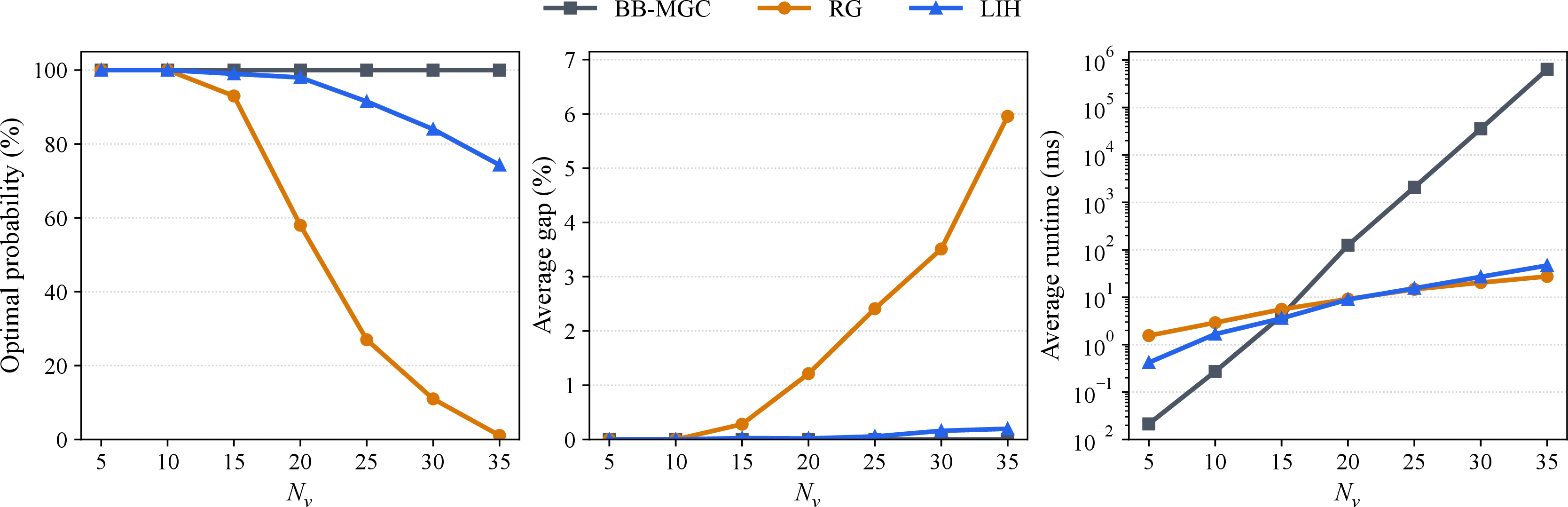
Table 4 summarizes all instances with an exact reference. BB-MGC certifies the optimum but requires \(22.83\) s on average. RG is much faster at \(13.75\) ms, but matches the optimum in only \(41.16\%\) of the instances and has an average gap of \(2.16\%\). LIH remains close to RG in runtime (\(18.19\) ms) while reaching \(91.25\%\) optimal probability and an average gap of only \(0.073\%\). When LIH is not optimal, its median positive gap is \(0.56\%\) and its 95th percentile positive gap is \(2.32\%\).
Effect of the Number of Vertices
| \(N_v\) | Comp. | RG opt. | LIH opt. | RG gap | LIH gap |
|---|---|---|---|---|---|
| 5 | 200 | \(100.0\%\) | \(100.0\%\) | \(0.00\%\) | \(0.00\%\) |
| 10 | 200 | \(100.0\%\) | \(100.0\%\) | \(0.00\%\) | \(0.00\%\) |
| 15 | 200 | \(93.0\%\) | \(99.0\%\) | \(0.28\%\) | \(0.026\%\) |
| 20 | 200 | \(58.0\%\) | \(98.0\%\) | \(1.21\%\) | \(0.019\%\) |
| 25 | 200 | \(27.0\%\) | \(91.5\%\) | \(2.41\%\) | \(0.056\%\) |
| 30 | 200 | \(11.0\%\) | \(84.0\%\) | \(3.51\%\) | \(0.160\%\) |
| 35 | 183 | \(1.1\%\) | \(74.3\%\) | \(5.96\%\) | \(0.198\%\) |
Table 5 and Fig. 8 show the node-scaling trend. The “Comp.” column gives the number of instances with a certified BB-MGC reference; at \(N_v=35\), 17 of 200 BB-MGC runs time out. RG’s optimal probability falls from \(100.0\%\) at \(N_v=10\) to \(1.1\%\) at \(N_v=35\), while LIH still reaches \(74.3\%\) with an average gap below \(0.2\%\). BB-MGC runtime grows to \(638.21\) s at \(N_v=35\); RG and LIH remain in the millisecond range, with averages of \(27.39\) ms and \(46.65\) ms.
Large-Node Comparison with Randomized Greedy
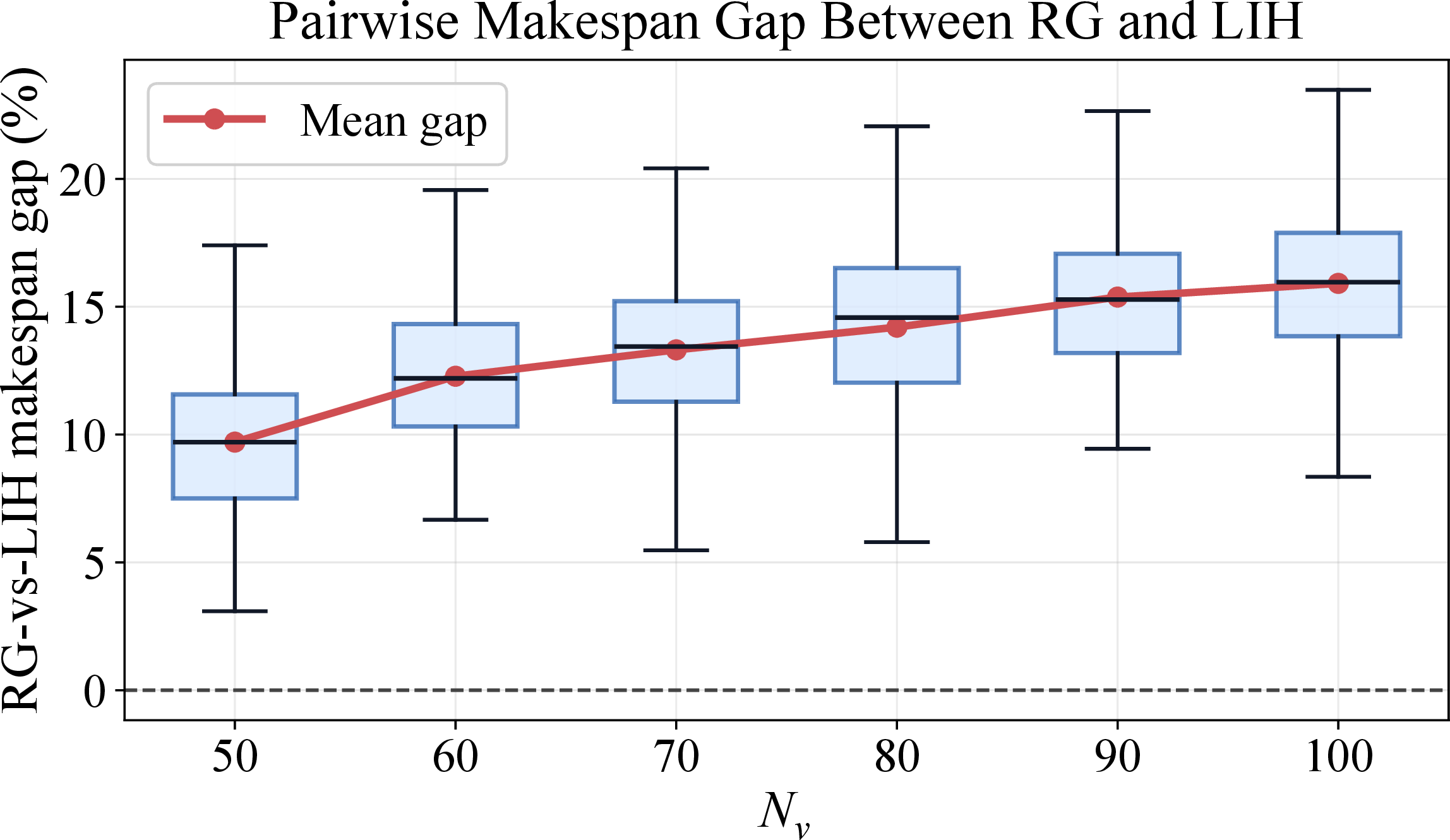
For larger instances, where BB-MGC is impractical, we compare LIH directly with RG for \(N_v=50,60,\ldots,100\), using 200 instances per setting under the default \(D=30\%\), \(R=5\%\), and Normal-weight configuration. Figure 9 shows that LIH obtains a smaller makespan in all 1200 pairwise comparisons. The average RG-to-LIH gap increases from \(9.70\%\) at \(N_v=50\) to \(15.91\%\) at \(N_v=100\), and LIH’s average compression exceeds RG by \(3.39\)–\(4.98\) percentage points. This supports the exact-reference trend: Lagrangian pricing becomes more valuable as the clique-combination space grows.
4.3 Sensitivity to Graph and Weight Parameters↩︎
Effect of Graph Density
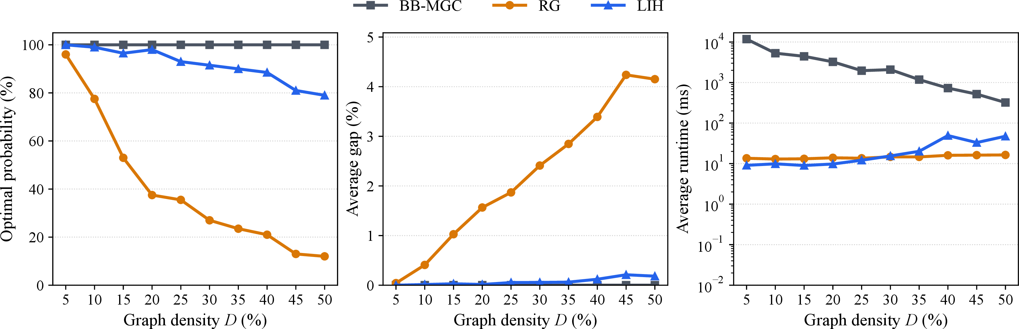
Figure 10 reports the effect of compatibility density. As \(D\) increases from \(5\%\) to \(50\%\), the exact baseline’s average compression rises from \(25.91\%\) to \(66.95\%\), but the grouping decision also becomes harder. RG’s optimal probability drops from \(96.0\%\) to \(12.0\%\), and its average gap grows from \(0.04\%\) to \(4.15\%\). LIH is less sensitive: its optimal probability stays between \(79.0\%\) and \(100.0\%\), and its average gap never exceeds \(0.21\%\).
Effect of Directed-Edge Ratio
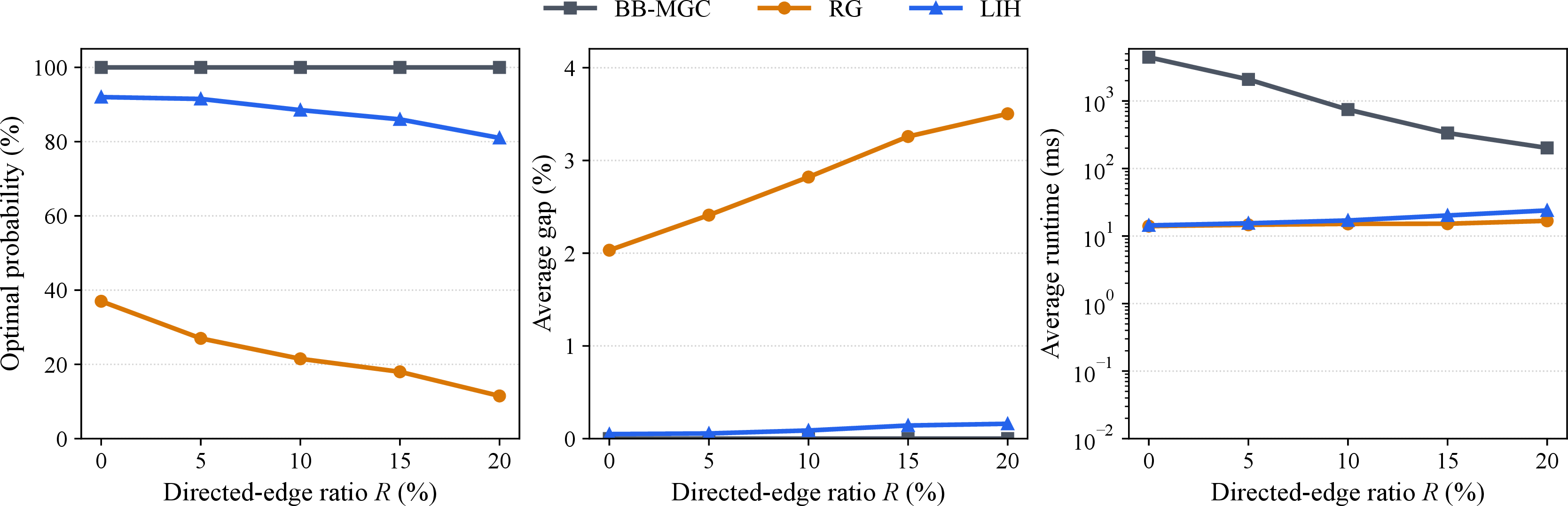
Figure 11 isolates precedence constraints. As \(R\) increases from \(0\%\) to \(20\%\), average exact compression decreases from \(58.29\%\) to \(52.12\%\), while BB-MGC runtime falls from \(4.44\) s to \(0.20\) s because ordering constraints reduce the coloring search space. RG’s optimal probability decreases from \(37.0\%\) to \(11.5\%\), with its average gap rising from \(2.03\%\) to \(3.50\%\). LIH maintains \(81.0\%\)–\(92.0\%\) optimal probability and keeps the average gap below \(0.17\%\).
Effect of Weight Distribution
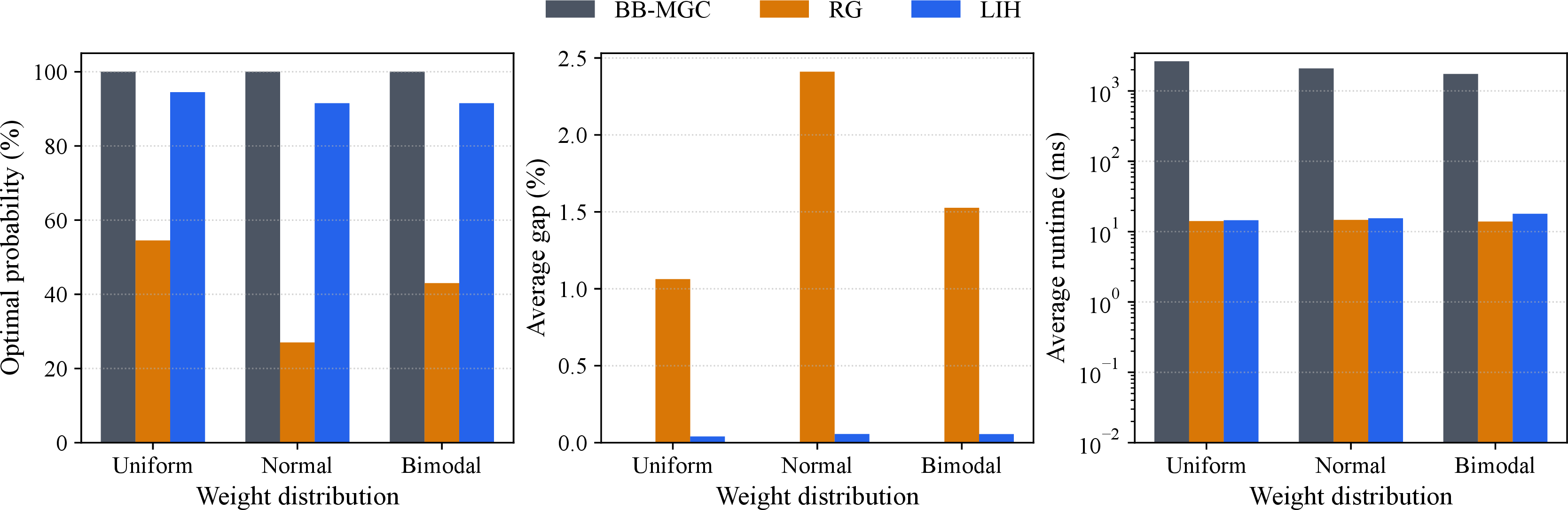
Figure 12 compares Uniform, Normal, and Bimodal weights. RG stays fast but its quality varies: the average gap is \(1.06\%\), \(2.41\%\), and \(1.53\%\), respectively. LIH is more stable, with optimal probabilities of \(94.5\%\), \(91.5\%\), and \(91.5\%\), and an average gap no larger than \(0.056\%\). Reduced-cost pricing therefore captures weighted savings more reliably than local insertion alone.
4.4 Discussion↩︎
Overall, BB-MGC is useful for certification but becomes expensive as the coloring search space expands. RG is lightweight, yet its local insertion decisions degrade with graph size, density, and precedence complexity. LIH adds Lagrangian pricing before feasibility repair, giving high optimal probability, very small gaps, and millisecond-level runtime in the exact-reference settings. On 50–100-node instances, LIH also consistently improves over RG in makespan and compression, supporting its use for static MPE batching when solution quality matters.
5 Case Study: From PLC Ladder Logic to MPE↩︎
This section reports an end-to-end case study that maps PLC ladder programs to the proposed MPE model, generates staged Verilog, and simulates the resulting HDL to measure control-cycle latency.
5.1 PLC Ladder Programs and Dependencies↩︎
Programmable Logic Controllers (PLCs) are widely used in industrial automation and embedded control, where deterministic scan behavior is essential. In each scan, the controller samples inputs, evaluates the ladder program, and updates outputs. Ladder Diagram (LD) represents this logic as rungs composed of contacts and coils: normally open contacts read a signal directly, normally closed contacts read its complement, and coils update memory variables or physical outputs.
During rung-by-rung execution, later rungs may observe values produced by earlier rungs in the same scan. For rung \(R_i\), let \(\mathrm{Read}(R_i)\) and \(\mathrm{Write}(R_i)\) denote the variables it reads and writes. If \(\mathrm{Write}(R_i)\cap \mathrm{Read}(R_j)\neq\emptyset\), then \(R_j\) depends on \(R_i\). Multiple writes to the same coil also preserve scan order. Interlocking-signal conflicts, such as complementary NO/NC reads of the same input or mutually exclusive control actions, are treated as compatibility constraints even when they do not form direct data dependencies.
Thus, ladder programs contain both local serial chains and independent branches. MPE exposes the legal within-scan parallelism without changing the observable PLC scan semantics.
5.2 SPG Modeling of PLC Ladder Logic↩︎
We model a ladder program by constructing the mixed graph \(G=(V,E,A)\) and the weight vector \(w\) used in Section 2. The construction has four steps.
Task extraction. Each rung, or each basic logic block inside a large rung, becomes a task vertex \(v\in V\). The vertex weight \(w_v\) is the estimated execution delay of that rung or logic block.
Precedence extraction. If a value written by \(R_i\) is read by \(R_j\), or if two writes must preserve scan order, we add a directed arc \((R_i,R_j)\in A\). The reachability relation in \((V,A)\) is later used to forbid batching two rungs that are connected by a direct or transitive dependence.
Compatibility extraction. Two vertices are connected by an undirected edge in \(E\) only when they have no precedence-path conflict, no interlocking-signal conflict, and no platform-specific conflict such as exclusive I/O access or a shared hardware resource that cannot be duplicated.
Batch optimization. The resulting graph is solved as an MPE instance. A selected clique represents one legal parallel execution batch, and the contracted graph gives the order in which batches are issued.
The implemented front end supports compact ladder descriptions and PLCOpen-style XML programs [20]. For XML input, each
program POU is converted into one SPG: coils or outVariable elements become vertices, upstream contacts provide read sets, scan-order write/read relations become directed arcs, and function blocks become weighted computation
dependencies or HDL module instances.
Table 6 gives a representative fragment. \(R_1\) writes \(C_1\), which is read by \(R_2\) and \(R_3\), so arcs \((R_1,R_2)\) and \((R_1,R_3)\) are added. \(R_4\) and \(R_5\) read \(I_2\) through complementary contacts, so their compatibility edge is omitted. The mapping is shown in Fig. 13.
| Rung | Read variables | Write variables | Graph constraint |
|---|---|---|---|
| \(R_1\) | \(I_1\) (NO) | \(C_1\) | Source rung |
| \(R_2\) | \(C_1,I_4\) (NO) | \(M_1\) | Arc \((R_1,R_2)\) |
| \(R_3\) | \(C_1,I_3\) (NO) | \(M_2\) | Arc \((R_1,R_3)\) |
| \(R_4\) | \(I_2\) (NC) | \(C_2\) | Incompatible with \(R_5\) |
| \(R_5\) | \(I_2\) (NO) | \(M_3\) | Incompatible with \(R_4\) |
Assume the rung weights are \[(w_{R_1},w_{R_2},w_{R_3},w_{R_4},w_{R_5})=(4,6,5,3,4).\] Serial execution has makespan \(4+6+5+3+4=22\). Applying LIH to this graph returns the following legal staged batching plan: \[\mathcal{C}=\bigl\{\{R_1,R_4\},\{R_2,R_3,R_5\}\bigr\}.\] The two stages preserve the dependencies from \(R_1\) to \(R_2\) and \(R_3\) and separate the interlocking pair \(R_4,R_5\). Under the staged batching semantics in Section 2, the makespan is \[T(\mathcal{C}) = \max\{4,3\}+\max\{6,5,4\} = 10.\] The example illustrates the weighted clique-partitioning objective: each batch is a feasible clique, and total time sums the slowest task in each batch.
5.3 FPGA-Oriented Parallel Realization↩︎
After LIH produces a legal batching plan, each batch is emitted as one FPGA execution stage. Contacts become signal reads or negations, LD operations become combinational logic or function-block instances, and coils are mapped to intermediate or output registers according to scan semantics.
The generated Verilog module uses a clocked start/done interface. At the start of a scan, physical inputs are sampled into input-image registers; a finite-state controller then issues the MPE stages in a topological order of
the contracted graph. All rungs in the current clique are evaluated in parallel, and their results are registered before the next stage. This preserves the PLC input/output boundary while extracting parallelism inside the execution phase.
5.4 Benchmark and Simulation Results↩︎
The evaluation uses six compact ladder kernels and 30 legitimate PLCOpen XML programs from the PLC-LD benchmark collection [20]7. The compact kernels cover representative dependency patterns; the XML programs test the full parsing, scheduling, HDL generation, and simulation pipeline.
| Benchmark | Graph | Cycles | Makespan | |||||||
|---|---|---|---|---|---|---|---|---|---|---|
| 2-4(lr)5-7(l)8-10 | \(|V|\) | \(|A|\) | \(|E|\) | PLC | HDL | C-spd. | \(T_s\) | \(T_p\) | W-spd. | |
| alarm/fault | 10 | 10 | 11 | 10 | 6 | 1.67 | 31 | 18 | 1.72 | |
| interlock | 5 | 2 | 7 | 5 | 3 | 1.67 | 22 | 10 | 2.20 | |
| motor_chain | 6 | 4 | 9 | 6 | 4 | 1.50 | 20 | 12 | 1.67 | |
| sensor_vote | 7 | 6 | 4 | 7 | 5 | 1.40 | 24 | 16 | 1.50 | |
| pid_bank | 7 | 6 | 12 | 7 | 4 | 1.75 | 38 | 16 | 2.38 | |
| sequence | 8 | 7 | 9 | 8 | 6 | 1.33 | 24 | 18 | 1.33 | |
| lassignment | 5 | 2 | 8 | 5 | 3 | 1.67 | 46 | 21 | 2.19 | |
| lassignment1 | 3 | 0 | 3 | 3 | 2 | 1.50 | 32 | 14 | 2.29 | |
| lexit | 7 | 6 | 15 | 7 | 4 | 1.75 | 62 | 29 | 2.14 | |
| lstart_cycle | 5 | 2 | 8 | 5 | 3 | 1.67 | 58 | 27 | 2.15 | |
| lstart_cycle1 | 3 | 0 | 3 | 3 | 2 | 1.50 | 44 | 20 | 2.20 | |
| lstart_eq | 5 | 2 | 8 | 5 | 3 | 1.67 | 49 | 21 | 2.33 | |
| lstart_le | 5 | 2 | 8 | 5 | 3 | 1.67 | 49 | 21 | 2.33 | |
| lstart_le1 | 3 | 0 | 3 | 3 | 2 | 1.50 | 35 | 14 | 2.50 | |
| lstart_lt | 3 | 0 | 3 | 3 | 2 | 1.50 | 35 | 14 | 2.50 | |
| lstart_lt1 | 3 | 0 | 3 | 3 | 2 | 1.50 | 25 | 9 | 2.78 | |
| lstop_eq | 5 | 2 | 8 | 5 | 3 | 1.67 | 49 | 21 | 2.33 | |
| lstop_eq1 | 3 | 0 | 3 | 3 | 2 | 1.50 | 35 | 14 | 2.50 | |
| lstop_ge | 5 | 2 | 8 | 5 | 3 | 1.67 | 49 | 21 | 2.33 | |
| lstop_ge1 | 3 | 0 | 3 | 3 | 2 | 1.50 | 35 | 14 | 2.50 | |
| lstop_gt | 5 | 2 | 8 | 5 | 3 | 1.67 | 49 | 21 | 2.33 | |
| lstop_gt1 | 3 | 0 | 3 | 3 | 2 | 1.50 | 35 | 14 | 2.50 | |
| lsub_function | 6 | 2 | 13 | 6 | 3 | 2.00 | 51 | 21 | 2.43 | |
| lsub_function1 | 6 | 2 | 13 | 6 | 3 | 2.00 | 51 | 21 | 2.43 | |
| lsub_function2 | 6 | 2 | 13 | 6 | 3 | 2.00 | 51 | 21 | 2.43 | |
| lsub_function3 | 4 | 0 | 6 | 4 | 2 | 2.00 | 37 | 14 | 2.64 | |
| lsubstitution_coil | 5 | 2 | 8 | 5 | 3 | 1.67 | 52 | 21 | 2.48 | |
| lsubstitution_coil1 | 3 | 0 | 3 | 3 | 2 | 1.50 | 38 | 14 | 2.71 | |
| lsubstitution_start | 5 | 2 | 8 | 5 | 3 | 1.67 | 51 | 21 | 2.43 | |
| lsubstitution_start1 | 3 | 0 | 3 | 3 | 2 | 1.50 | 37 | 14 | 2.64 | |
| lsubstitution_stop | 5 | 2 | 8 | 5 | 3 | 1.67 | 51 | 21 | 2.43 | |
| lsubstitution_stop1 | 3 | 0 | 3 | 3 | 2 | 1.50 | 37 | 14 | 2.64 | |
| lvalue_filtering | 5 | 2 | 8 | 5 | 3 | 1.67 | 62 | 29 | 2.14 | |
| lvalue_filtering1 | 3 | 0 | 3 | 3 | 2 | 1.50 | 48 | 22 | 2.18 | |
| lvalves_handler | 5 | 2 | 8 | 5 | 3 | 1.67 | 46 | 21 | 2.19 | |
| lvalves_handler1 | 3 | 0 | 3 | 3 | 2 | 1.50 | 32 | 14 | 2.29 | |


Figure 13: Case-study mapping from a ladder fragment to the corresponding SPG. In Fig. 13 (b), gray edges are compatibility edges, blue arrows are precedence arcs, and the dashed red segment marks the omitted compatibility edge caused by an interlocking-signal conflict..
Table 7 gives the per-program comparison. Across the six compact ladder kernels, MPE reduces weighted makespan by \(42.12\%\) on average; PID-bank and interlock gain most from compatible branches, while sequence control is limited by longer scan-order chains.
For the PLCOpen XML benchmarks, the pipeline generated one SPG, one LIH schedule, and one Verilog module per program. All 30 generated modules compiled with the common HDL library and completed ModelSim simulation. The measured controller latency falls from \(4.27\) PLC scan cycles to \(2.57\) HDL cycles on average, giving a \(1.642\times\) cycle speedup and a \(38.54\%\) cycle reduction. In the weighted MPE metric, the same benchmarks achieve \(2.399\times\) average speedup, or a \(58.10\%\) staged-makespan reduction. Thus, the selected cliques are not only scheduling abstractions; they translate into executable HDL stages that preserve PLC scan semantics.
6 Related Work↩︎
This section follows the same progression as the paper. We first review task-graph and series-parallel scheduling models related to the MPE formulation, then discuss mixed graph coloring and clique partitioning, followed by column models and Lagrangian relaxation. We finally relate the resulting batching model to FPGA-based embedded control.
6.1 Task-Graph and Series-Parallel Scheduling↩︎
Precedence-constrained task-graph scheduling is NP-hard in general [15]. Classical heterogeneous DAG schedulers such as HEFT [21] and PEFT [22] map and order tasks on a fixed processor set while respecting precedence and communication costs. Recent work has extended this line to FPGA-based heterogeneous real-time systems [23], preloaded shared-bus heterogeneous platforms [24], typed DAG tasks on heterogeneous multicores [25], and energy-efficient scheduling on heterogeneous embedded platforms [26]. These studies emphasize resource assignment and schedule construction on specified heterogeneous resources, whereas MPE abstracts a sufficiently provisioned FPGA stage and asks which compatible tasks can be batched without violating precedence-induced acyclicity.
Series-parallel graphs provide additional structure. Their recognition and decomposition are well studied [27], and scheduling methods have exploited this structure for processor-constrained approximation and static scheduling [2], [28]. In contrast, MPE forms parallel batches under abundant hardware parallelism, with feasibility defined by both precedence and compatibility plus acyclicity after contraction.
6.2 Mixed Graph Coloring and Clique Partitioning↩︎
The MPE formulation is closely related to mixed graph coloring and clique partitioning. A mixed graph contains both undirected edges and directed arcs, and mixed graph coloring uses undirected edges to encode conflicts and directed arcs to encode ordering constraints [29]. This viewpoint is widely used in scheduling models based on disjunctive or mixed graphs. Kouider and Ait Haddadene [19] proposed a bi-objective branch-and-bound algorithm for unit-time job shop scheduling through mixed graph coloring. We use a weighted adaptation of this exact mixed-coloring framework as the BB-MGC baseline in the experiments.
Our formulation is related but not identical. In MPE, undirected edges denote compatibility, so the mixed-coloring instance is obtained by complementing the edge set. The objective is also weighted: a batch costs the maximum execution time of its tasks, matching FPGA-style concurrent execution. This gives an exact BB-MGC baseline for small instances, but its branch-and-bound search becomes expensive as feasible color classes grow.
6.3 Column Models and Lagrangian Relaxation↩︎
The exact MPE formulation can be viewed as a set-partitioning model over all feasible cliques. Such column-based formulations are common in large-scale combinatorial optimization, but the number of columns can be exponential. Branch-and-price methods address this difficulty by solving a restricted master problem and generating useful columns through reduced costs [30]. Lagrangian relaxation provides another classical way to handle hard coupling constraints by moving them into the objective with multipliers [17], [18].
LIH follows this philosophy but targets MPE. It constructs a pricing-filtered pool of SPG-aware cliques, uses Lagrangian multipliers as vertex prices, and repairs the relaxed selection into an acyclic clique partition. This retains a global pricing signal without the cost of full branch-and-price.
6.4 FPGA-Based Embedded Control↩︎
FPGAs are widely used in industrial and safety-critical control because they provide deterministic timing, fine-grained parallelism, and isolation. Prior work surveys FPGA design for industrial control [8] and fault-tolerant SRAM-based FPGA systems [14]. Recent studies also accelerate PLC and embedded-control workloads, such as multi-PID FPGA implementations for reducing PLC scan time [5], deterministic parallelization of legacy control code [6], and shared-resource effects on real-time microcontrollers [7].
These works motivate hardware acceleration, while our focus is the graph-level batching problem that decides which compatible tasks can share an FPGA execution stage. Work on heterogeneous real-time FPGA systems, such as MESSI [23], and accelerator-scheduling surveys [31] mainly emphasize resource allocation and deadline analysis. We instead study a sufficiently provisioned setting where dependency and compatibility determine the available parallelism.
7 Conclusion↩︎
This paper studied Maximum Parallel Execution (MPE) for series-parallel task graphs motivated by FPGA acceleration of embedded control programs. We modeled MPE as a weighted clique-partitioning problem: compatible tasks share a parallel batch, and selected batches are issued in a topological order of the contracted precedence graph. The proposed LIH algorithm combines SPG-aware candidate generation, warm-up pricing screening, Lagrangian pricing, feasibility repair, and local refinement.
The experiments show that LIH keeps the solution quality close to the exact BB-MGC reference while remaining in the millisecond range. Across comparable instances, LIH matches the optimum in \(91.25\%\) of cases with an average gap of \(0.073\%\), whereas the exact baseline becomes costly as the coloring search space grows. On 50–100-node instances, LIH consistently improves over the randomized greedy baseline, indicating that the pricing signal becomes more useful as the grouping space expands.
The PLC ladder case study further connects the graph model to HDL generation and cycle-level simulation, showing that selected cliques can be realized as deterministic FPGA stages. Future work will incorporate explicit hardware resources, communication overheads, and more detailed FPGA placement or safety-partitioning requirements.
References↩︎
Jinghao Sun and Xiuzhen Cheng are with the School of Computer Science and Technology, Shandong University, Qingdao 266237, China (e-mail: jhsun@sdu.edu.cn; xzcheng@sdu.edu.cn).↩︎
Zhenchu Hu and Ye Ma are with the School of Computer Science and Technology, Dalian University of Technology, Dalian 116024, China (e-mail: huzhenchu@mail.dlut.edu.cn; yema@dlut.edu.cn).↩︎
Bo Tang is with Weichai Power Co., Ltd., Weifang 261061, China. (e-mail: b.tang@hotmail.com)↩︎
Qingxu Deng is with the School of Computer Science and Engineering, Northeastern University, Shenyang 110004, China (e-mail: dengqx@mail.neu.edu.cn).↩︎
Corresponding author: Ye Ma (e-mail: yema@dlut.edu.cn).↩︎
Strictly speaking, the model used in this paper is an augmented SPG rather than a conventional SP graph. The series-parallel restriction is imposed on the directed precedence component \((V,A)\); the model additionally includes undirected compatibility edges \(E\), vertex execution times \(w_v\), and the staged-batching semantics with contracted-graph acyclicity used for MPE.↩︎