¹

1 Introduction and main results↩︎

The Discrete Kirchhoff Triangle (DKT) is a finite-element based numerical scheme for discretizing variational problems posed in subspaces of the Sobolev space \(H^2\), originally invented and developed for mechanical models of plate bending. Therein, the complicated design and implementation of conforming finite element methods (FEM) is circumvented by introducing a separate variable \(\theta_h\) representing a discrete gradient. The solution \(u\) is approximated by \(u_h\) and its gradient \(\nabla u\) by \(\theta_h\), and the quantities \(\nabla u_h\) and \(\theta_h\) are coupled through discrete conditions and not through pointwise identity. The resulting scheme is easy to implement with standard finite element assembly, once the discrete coupling is encoded in an additional matrix. In plate analysis, the assumption that the displacement gradient \(\nabla u\) equals the in-plate rotation \(\theta\) is known as Kirchhoff’s hypothesis, explaining the nomenclature of the DKT element, which enforces this constraint discretely. This note is devoted to a structural analysis of the DKT paradigm for a larger class of low-order discretizations, which we expose for the biharmonic equation under clamped boundary conditions for the sake of simplicity of the presentation.

Let \(\Omega\subset \mathbb{R}^{n}\) be an open, bounded, connected Lipschitz polytope in dimension \(n\in\{2,3\}\), with outer unit normal \(\nu\). Given a right-hand side \(f\in L^2(\Omega)\), the weak form of the problem \(\Delta^2 u = f\) in \(\Omega\) subject to the clamped boundary condition \(u=\nabla u\cdot\nu=0\) on \(\partial \Omega\) seeks \(u \in V \mathrel{\vcenter{:}}= H^2_0(\Omega)\) with \[\begin{align} \label{def:continuous-problem} a(u, v) \mathrel{\vcenter{:}}= (D^2 u, D^2 v)_{L^2(\Omega)} = (f, v)_{L^2(\Omega)} \quad\text{for any } v \in V. \end{align}\tag{1}\] Let \(\mathcal{T}\) be a regular triangulation of \(\Omega\) into simplices and let the space \(V_h\) consist of piecewise polynomial functions over \(\Omega\), while \(\Theta_h\) is a space of piecewise polynomial vector fields. Assume we are given a linear discrete gradient map \(\nabla_h : V_h \to \Theta_h\) that defines the discrete Hessian \(D^2_h \mathrel{\vcenter{:}}= D_\mathrm{pw}\circ \nabla_h\). Here and throughout this work, the index \(\mathrm{pw}\) attached to a differential operator denotes its piecewise action with respect to a given mesh \(\mathcal{T}\). Then the discrete problem seeks a solution \(u_h \in V_h\) to \[\begin{align} \label{def:discrete-problem} a_h(u_h,v_h) = (f,v_h)_{L^2(\Omega)} \quad\text{for any } v_h \in V_h \end{align}\tag{2}\] with the bilinear form \[\begin{align} a_h(u_h,v_h) \mathrel{\vcenter{:}}= (D_h^2 u_h, D_h^2 v_h)_{L^2(\Omega)}. \end{align}\] The seminorm induced by \(a_h\) is denoted by \(\|\cdot\|_{h}\). If \(V_h\subset H^1_0(\Omega)\) is satisfied, we can relax the conditions on \(f\) to \(f\in H^{-1}(\Omega)\) in 1 –2 .

The main result of this note is that the error \(\sigma-\sigma_h\) in the \(L^2\) norm between \(\sigma \mathrel{\vcenter{:}}= D^2 u\) and \(\sigma_h \mathrel{\vcenter{:}}= D_h^2 u_h\) is bounded from above by the best-approximation of \(\sigma\) by piecewise constants, written \(\Pi_0\sigma\), plus oscillations of the right-hand side \(f\), provided the following conditions are satisfied. In what follows, we denote by \(\mathcal{F}\) the set of faces of \(\mathcal{T}\) and by the brackets \([\cdot]_F\) the jump of a piecewise polynomial function across a face \(F\in\mathcal{F}\). For boundary faces, the brackets denote the trace. The \(L^2\) norm over a measurable set \(\omega\) is written as \(\|\cdot\|_\omega\) with the convention \(\|\cdot\| \mathrel{\vcenter{:}}= \|\cdot\|_\Omega\).

As a consequence of (C1)–(C4), the bilinear form \(a_h\) is positive definite over \(V_h\). In fact, if \(D^2_h v_h = 0\), then \(\nabla_h v_h\) is piecewise constant, (C1) shows that it equals zero. From (C3), we infer \(D^2_\mathrm{pw}v_h \equiv 0\). Hence, (C4) implies \(\nabla_\mathrm{pw}v_h \equiv 0\) and so, \(v_h\) is piecewise constant. By (C2), \(v_h \equiv 0\). The positivity of \(a_h\) shows that 2 possesses a unique discrete solution \(u_h\). The error estimate reads:

The oscillations \(\operatorname{osc}(f,\mathcal{T})\) are described in Section 2, 1 below and are defined for \(f\in H^{-1}\) provided \(V_h\) is a subspace of \(H^1_0(\Omega)\). Otherwise, they correspond to the usual \(L^2\)-based oscillations.

An immediate consequence is an error bound under minimal regularity assumptions for several known schemes satisfying Condition C. First, the error bound applies to the DKT element and reveals that the \(H^3\) regularity assumed in prior contributions [1]–[3] is not a qualitative limitation to the method. Second, Condition C as a set of structure conditions allows for a canonical generalization of the DKT element to three dimensions, which leads to a simple low-order scheme not documented so far in the literature. The application of the error bounds to several other nonconforming methods is possible and briefly commented on in Section 8. Error estimates in weaker norms are provided in 1 in Section 3 below, and an adaptation of the error bound for a singularly perturbed problem is given as 2.

The conditions furthermore allow for a reliable a posteriori error bound.

We note that the first bound (reliability) is implied by Condition C, while the second bound (efficiency) has been known [4] and is not a new contribution here.

Error estimates under minimal regularity assumptions were studied in [5]–[7] and more abstractly in [8] for classical nonconforming or discontinuous Galerkin schemes. The error analysis in this work shows that DKT elements and many other known nonconforming methods for the biharmonic operator share structural conditions that are sufficient for quasi-best approximation of the Hessian by piecewise constants. We furthermore describe in 6 a connection to two-dimensional stable pairs for the Stokes equations. This gives room for a re-interpretation of DKT-like elements as discrete stream functions of known discretely divergence-free functions, rather than an ad-hoc construction for plate analysis only.

Throughout this article, standard notation on Lebesque and Sobolev spaces is employed with the \(L^2\) inner product \((\cdot,\cdot)_\omega\) over a measurable subset \(\omega\) of \(\mathbb{R}^n\) and the \(L^2\) norm \(\|\cdot\|_\omega\). If \(\omega=\Omega\), the index is dropped. The space of functions over a set \(T\) that are polynomial of degree at most \(k\) is denoted as \(P_k(T)\), and \(P_k(\mathcal{T})\) denotes the space of functions that belong to \(P_k(T)\) when restricted to any simplex \(T\) of the triangulation \(\mathcal{T}\). The \(L^2\) projection onto \(P_0(\mathcal{T})\) is denoted by \(\Pi_0\). The diameter of a set \(\omega\) is denoted by \(h_\omega\), and \(h\) denotes the piecewise constant mesh-size function with respect to a triangulation \(\mathcal{T}\) such that \(h|_T=h_T\) for any simplex \(T\in\mathcal{T}\); \(h_{\max} = \|h\|_{L^\infty(\Omega)}\) is the maximal mesh-size. An inequality \(A\leq CB\) with a generic constant \(C\) that may depend on the shapes in the triangulation \(\mathcal{T}\) but not on the mesh size, is denoted by \(A\lesssim B\), and we write \(A\approx B\) for \(A\lesssim B \lesssim A\). The Frobenius inner product of matrices \(M,N\) is denoted by the colon, \(M:N\).

The remaining parts of this paper are organized as follows. 2 discusses several preliminary results implied by Condition C, including the construction of smoothing operators. 3 is devoted to the proof of 1 as well as its consequences such as lower-order estimates and extension to singularly perturbed biharmonic operators. The proof of 2 is given in 4. The results are applied to DKT elements in 5. 6 discusses the relation to pressure-robust discretizations of planar Stokes flow. Two and three dimensional numerical benchmarks are provided in 7. Some comments on other classical nonconforming FEM in 8 conclude this note.

2 Consequences of the structure conditions↩︎

In this section, we derive some direct conclusions from Condition C and prove the existence of a smoothing operator \(J\). This operator allows to quantify consistency and oscillations of the right-hand side. Such operators were constructed in more specific situations by [9]–[12], for example. As a preliminary step, we discuss some basic properties around (C1)–(C5) on local equivalence of the classical gradient \(\nabla\) and the discrete gradient \(\nabla_h\) acting on discrete functions from \(V_h\). A first consequence of (C3) is the equivalence of the local seminorms \[\label{e:normeq} \|D^2 \bullet\|_{T} \approx \|D^2_h \bullet\|_{T}\tag{3}\] for discrete functions. Condition (C3) is satisfied in most reasonable discrete schemes because of the following. Suppose that \(\nabla_h v_h|_T\) being affine implies that \(v_h|_T\) is a quadratic polynomial and \(\nabla_h v_h|_T = \nabla v_h|_T\). Then, (C3) is satisfied. The hidden constant therein depends on the shape of the simplex. Under the condition that these constants are invariant under scaling and translation, they remain uniformly bounded for families of triangulations involving finite many shapes, such as the ones created by the newest-vertex bisection. Another consequence of (C3)–(C4) is the local equivalence of the gradient and the discrete gradient, namely \[\label{e:normeq95nabla} \|\nabla \bullet\|_{T} \approx \|\nabla_h \bullet\|_{T},\tag{4}\] which can be proven by combining (C4) with the triangle inequality, (C3), and an inverse estimate. We further note that (C3) implies the following local equivalence \[\label{e:ba-loc} \|(1 - \Pi_0) D^2 v_h\|_T \approx \|(1 - \Pi_0) D_h^2 v_h\|_T.\tag{5}\]

Let \(\{\cdot\}_F\) denote the average of the values from the simplices adjacent to \(F \in \mathcal{F}\) (for boundary faces it denotes the trace) and \(\nu_F\) is a given normal unit vector of \(F\) (for boundary faces it coincides with the outer normal unit vector \(\nu\) of \(\Omega\)).

As a direct consequence of the foregoing lemma and (C3), we note that the map \(J \circ Q_h\) defines a quasi-interpolation into \(C^1\) conforming finite elements with local approximation properties.

The following result is the main ingredient for the error analysis.

Based on the operator \(J\), we define the data oscillation \(\operatorname{osc}(f,\mathcal{T})\) of \(f\) as follows.

The following result shows that the classical data oscillation provides an upper bound of the quantity defined in 1.

3 A priori error analysis↩︎

This section is devoted to the proof of 1 and extensions of the error analysis to weaker norms (1) and a singular perturbation problem (2). Recall the notation \(\sigma=D^2 u\) and \(\sigma_h=D_\mathrm{pw}\nabla_h u_h=D^2_h u_h\) for the solutions \(u\) and \(u_h\) to 1 and 2 . The proof of 1 utilizes the following Galerkin projection onto the space of piecewise quadratic functions. For any \(v \in V\), the piecewise quadratic function \(G_h v \in P_2(\mathcal{T})\) is the unique solution to \[\begin{align} (D^2_\mathrm{pw}G_h v, D^2_\mathrm{pw}p)_\Omega &= (D^2 v, D^2_\mathrm{pw}p)_{\Omega} &&\text{for all } p \in P_2(\mathcal{T}),\\ (G_h v, q)_\Omega &= (v, q)_\Omega &&\text{for all } q \in P_1(\mathcal{T}). \end{align}\] By design, \(\|D^2(v - G_h v)\| = \min_{p \in P_2(\mathcal{T})} \|D^2_\mathrm{pw}(v - p)\|\) and, since the space of piecewise Hessians of the piecewise quadratic functions equals the space of piecewise constant symmetric-matrix valued functions, written \(D^2_\mathrm{pw}P_2(\mathcal{T}) = P_0(\mathcal{T};\mathbb{S})\), and \(D^2 v\) is symmetric pointwise a.e., we deduce \[\begin{align} \label{eq:Galerkin-err} \|D^2(v - G_h v)\| = \|(1 - \Pi_0) D^2 v\|. \end{align}\tag{14}\] We proceed with the proof of 1.

A direct consequence of 1 is the estimate \[\begin{align} \label{ineq:alt-err-est} \|\sigma_h - D^2 J u_h\| + \|\sigma - D^2 J u_h\| \lesssim \|(1 - \Pi_0) \sigma\| + \operatorname{osc}(f,\mathcal{T}) \end{align}\tag{16}\] with the triangle inequality, 3, and the continuity of \(J\). This shows that \(D^2 J u_h\) is a feasible approximation of \(\sigma\) and \(\|\sigma_h - D^2 J u_h\|\) is an efficient contribution of a posteriori error estimators. Another consequence of 1 is the quasi-optimality, up to data oscillations, of \(\|\sigma - \bar\sigma_h\|\) with the piecewise constant function \(\bar\sigma_h \mathrel{\vcenter{:}}= \Pi_0 \sigma\), namely \[\begin{align} \label{ineq:q-opt-pi0} \|\sigma - \bar\sigma_h\| \lesssim \|(1 - \Pi_0) \sigma\| + \operatorname{osc}(f,\mathcal{T}). \end{align}\tag{17}\] Other consequences of 1 are lower-order estimates as well as error estimates for the singular perturbed problem. Regarding the former, we focus, for the sake of brevity, on \(H^1\) estimates and mention that the arguments below also enable \(H^s\) estimates for any \(0 \leq s < 2\). For low-order methods we do not expect higher convergence rates in norms weaker than \(H^1\), cf. [19]. We assume the existence of \(0 < \delta \leq 1\) such that the solution to \(\Delta^2 z = g\) for any given \(g \in H^{-1}(\Omega)\) enjoys the elliptic regularity \(z \in H^{2 + \delta}(\Omega)\) with \[\begin{align} \label{ineq:elliptic-regularity} \|z\|_{H^{2 + \delta}} \lesssim \|g\|_{H^{-1}(\Omega)}. \end{align}\tag{18}\] In the two-dimensional case, such estimates are provided in [20], [21]. Recall the data oscillation \(\operatorname{osc}(f,\mathcal{T})\) from 1. Upper bounds are given in 5 and we abbreviate them by \(\widetilde{\operatorname{osc}}(f,\mathcal{T})\).

In the remaining parts of this section, we extend the a priori error bound of 1 to the case of a parameter-dependent problem. Given \(\varepsilon > 0\), the singular perturbed biharmonic problem seeks the unique solution \(u \in V\) to \[\begin{align} \label{def:a-singular-perturbed} a_\varepsilon(u,v) \mathrel{\vcenter{:}}= \varepsilon^2 (D^2 u, D^2 v)_\Omega + (\nabla u, \nabla v)_\Omega = (f,v)_\Omega \quad\text{for any } v \in V. \end{align}\tag{24}\] The scalar product \(a_\varepsilon\) induces the weighted norm \(\|\bullet\|_\varepsilon\) in \(V\). The discrete problem seeks \(u_h\in V_h\) such that \[\begin{align} \label{def:ah-singular-perturbed} a_{\varepsilon,h}(u_h,v_h) \mathrel{\vcenter{:}}= \varepsilon^2(D^2_h u_h, D^2_h v_h)_\Omega + (\nabla_\mathrm{pw}u_h, \nabla_\mathrm{pw}v_h)_\Omega = (f,v_h)_\Omega \end{align}\tag{25}\] for any \(v_h \in V_h\). We endow \(V_h\) with the weighted norm \(\|\bullet\|_{\varepsilon,h}\) induced by \(a_{\varepsilon,h}\). Throughout this discussion, all constants hidden in the notation \(\lesssim\) are independent of \(\varepsilon\). For the sake of brevity, we only carry out the analysis for \(\varepsilon \leq h_{\max}\) since the case \(h_{\max} < \varepsilon\) is simpler, cf. 4 for further details. In addition to (C1)–(C5), we will assume continuity of trial functions as in 3 and, for simplicity, quasi-uniform meshes.

As consequence of 6, we obtain strengthened versions of previous results. First, any \(v \in V\) satisfies \[\begin{align} \label{ineq:qi-singular-perturbed} \varepsilon\|D^2(v - J Q_h v)\| \lesssim \varepsilon\|(1 - \Pi_0) D^2 v\| + \|\nabla(v - Q_h v)\| + \|\nabla v - \nabla_h Q_h v\| \end{align}\tag{27}\] from 26 , the weighted trace inequality, (C5), and the triangle inequality. Second, any \(v_h,w_h \in V_h\) and \(p \in P_2(\mathcal{T})\) satisfy \[\begin{align} \label{ineq:d-cons-singular-perturbed} \varepsilon^2|(D_\mathrm{pw}^2 p, D_h^2 v_h - D^2 J v_h)_{\Omega}| \lesssim \varepsilon\|D^2_\mathrm{pw}(p - J w_h)\| \|v_h\|_{\varepsilon,h}. \end{align}\tag{28}\] To prove this, we apply the trace inequality to the bound prior to 11 to obtain \[\begin{align} &\varepsilon^2|(D_\mathrm{pw}^2 p, D_h^2 v_h - D^2 J v_h)_{\Omega}|\\ &\qquad\lesssim \varepsilon^2(\|h^{-1/2} A\| + \|A\|^{1/2}\|D_\mathrm{pw}A\|^{1/2}) (\|h^{-1/2}B\| + \|B\|^{1/2}\|D_\mathrm{pw}B\|^{1/2}) \end{align}\] with the abbreviation \(A \mathrel{\vcenter{:}}= \nabla_h v_h - \nabla J v_h\) and \(B \mathrel{\vcenter{:}}= D^2_\mathrm{pw}(p - J w_h)\). Since \(B\) is a piecewise polynomial function in \(\hat{\mathcal{T}}\), a triangulation with maximal mesh-size \(\hat{h}_{\max} \approx \varepsilon\), an inverse estimate shows \(\|h^{-1/2}B\| + \|B\|^{1/2}\|D_\mathrm{pw}B\|^{1/2} \lesssim \varepsilon^{-1/2}\|B\|\). From this, the foregoing displayed formula, the Young inequality \(\|A\|^{1/2}\|D_\mathrm{pw}A\|^{1/2} \leq \varepsilon^{-1/2}\|A\| + \varepsilon^{1/2}\|D_\mathrm{pw}A\|\), and the continuity of \(J\), we infer 28 . Finally, for \(f \in L^2(\Omega)\), we have the bound \[\begin{align} \label{ineq:osc-singular-perturbed} \operatorname{osc}(f,\mathcal{T}) \lesssim \|h(1 - \Pi_0) f\| \end{align}\tag{29}\] on the data oscillation by a Poincaré inequality with 6 and the continuity of \(J\). In the following, we abbreviate, for any \(v \in V\), \[\begin{align} \mathcal{R}(v) \mathrel{\vcenter{:}}= \|(1 - \Pi_0) \nabla v\| + \|\nabla(v - Q_h v)\| + \|\nabla v - \nabla_h Q_h v\|. \end{align}\]

To derive convergence rates from the a priori error estimate of 2, we need explicit knowledge on the degrees of freedom of the discrete trial space \(V_h\). We refer to 3 for an exemplary application to DKT elements. If \(h_{\max} \leq \varepsilon\), then we obtain the following a priori error estimate.

4 A posteriori error analysis↩︎

This section is devoted to the proof of the a posteriori error bound of 2. With the abbreviation \(\bar\sigma_h=\Pi_0\sigma_h\), we define the error estimator \[\begin{align} \label{e:mudef} \mu^2 \mathrel{\vcenter{:}}= \|&h^2 (f - \operatorname{div}_\mathrm{pw}\operatorname{div}_\mathrm{pw}\sigma_h)\|^2 + \|\operatorname{skw}\,\sigma_h\|^2 + \|\sigma_h - \bar\sigma_h\|^2 \nonumber\\ &+ \sum_{\substack{F \in \mathcal{F}\\ F\subset\partial\Omega}} h_F\|[\sigma_h^{\mathit{tang}}]_F\|_F^2 + \sum_{\substack{F \in \mathcal{F}\\ F\not\subset\partial\Omega}} \Big(h_F\|[\sigma_h]_F\|_F^2 + h_F^3\|[\operatorname{div}_\mathrm{pw}\sigma_h \cdot \nu_F]_F\|_F^2\Big), \end{align}\tag{31}\] where \(\sigma_h^{\mathit{tang}} \mathrel{\vcenter{:}}= \sigma_h(I_{n\times n}-\nu_F\nu_F^\top)\) denotes the tangential component of \(\sigma_h\). Here and throughout this section, \(\operatorname{skw} M\) denotes the skew-symmetric part of a matrix \(M\), while \(\operatorname{sym} M\) is its symmetric part.

5 Discrete Kirchhoff triangle and its generalization to three space dimensions↩︎

We apply the results from prior sections to the DKT setting. The method for \(n=2\) was proposed in [26] and described and analyzed in [1], [3]. Our description covers the case \(n=3\) as well and leads to a very simple low-order scheme in three space dimensions, which extends the known element by maintaining the underlying idea. The error analysis simultaneously covers the cases \(n\in\{2,3\}\).

Given a simplex \(T \subset \mathbb{R}^n\), \(n \in \{2,3\}\), with the vertices \(z_j\) for \(j = 1, \dots, n+1\) and the midpoints \(a_{jk\ell} \mathrel{\vcenter{:}}= (z_j + z_k + z_\ell)/3\) for \(1 \leq j < k < \ell \leq n+1\), recall from [27] that any cubic polynomial \(p\) is uniquely determined by the nodal values and the values of its first derivatives at the vertices \(z_j\), \(1 \leq j \leq n+1\) as well as the nodal values at \(a_{jk\ell}\). For each triplet \(j,k,\ell\), let \[\begin{align} \psi_{jk\ell}(p) \mathrel{\vcenter{:}}= 6p(a_{jk\ell}) - \sum\nolimits_{m \in \{j,k,\ell\}} (2p(z_m) - \nabla p(z_m) \cdot (z_m - a_{jk\ell})). \end{align}\] We define the reduced set \[\begin{align} P_3^-(T) \mathrel{\vcenter{:}}= \{p \in P_3(T) : \psi_{jk\ell}(p) = 0 \text{ for any } 1 \leq j < k < \ell \leq n+1\} \end{align}\] of cubic polynomials by removing the degrees of freedom associated with the nodal evaluation at \(a_{jk\ell}\), \(1 \leq j < k < \ell \leq n+1\). Thus, any \(p \in P_3^-(T)\) is uniquely defined by prescribing the nodal values and first derivatives at the \(n+1\) vertices and so, \(\dim P_3^-(T) = (n+1)^2\) [27]. Furthermore, let \[\begin{align} \Theta_h(T) \mathrel{\vcenter{:}}= \{\theta_h \in P_2(T)^n : \theta_h \cdot \nu_F \in P_1(F) ~\text{for any face } F \text{ of } T\}. \end{align}\] Recall that \(\theta_h \in P_2(T)^n\) is uniquely defined by the values at all vertices and midpoints of all edges of \(T\). The \(n\) values at the midpoint of an edge \(E\) are fixed in \(n-1\) linear independent directions from the side conditions \(\theta_h \cdot \nu_F \in P_1(F)\) on \(n-1\) adjacent faces. Thus, only the tangential direction \(t_E\), \(\theta_h(m_E)\cdot t_E\), remains as a degree of freedom in the midpoint \(m_E\) of \(E\). Hence, any \(\theta_h \in \Theta_h(T)\) is uniquely defined by the values at the vertices and midpoints of all edges along the tangential direction \(t_E\). This leads to \(\dim \Theta_h(T) = n(n+1) + n(n+1)/2 = 3n(n+1)/2\).

The discretization utilizes the DKT element of [26] with the discrete space \[\begin{align} V_h &\mathrel{\vcenter{:}}= \{v \in H^1_0(\Omega) : v|_T \in P_3^-(T) \;\text{ for all } T \in \mathcal{T},\\ &\qquad\nabla v \text{ is continuous at all vertices and 0 at all boundary vertices}\} \end{align}\] and reconstructs the gradient in \[\begin{align} \Theta_h \mathrel{\vcenter{:}}= \{\theta_h \in [H^1_0(\Omega)]^n : \theta_h|_T \in \Theta_h(T)\}. \end{align}\] The discrete gradient operator \(\nabla_h : V_h \to \Theta_h\) maps \(v_h \in V_h\) onto \(\nabla_h v_h \in \Theta_h\) with \[\begin{align} \nabla_h v_h(z) &= \nabla v_h(z) &&\text{for any vertex } z,\tag{39}\\ \nabla_h v_h(m_E) \cdot t_E &= \nabla v_h(m_E) \cdot t_E &&\text{for any edge } E \text{ with midpoint }m_E \tag{40} . \end{align}\] We proceed by verifying conditions (C1)–(C5) for this method. The properties (C1) and (C2) follow from the definition of \(V_h\), whereas (C3)–(C5) follow from the next results.

Since the DKT element satisfies (C1)–(C5) and \(H^1_0(\Omega)\) conformity, we obtain the following error bounds. Recall that \(\sigma_h = D^2_h u_h = D \nabla_h u_h\).

To simplify the implementation, we can modify the discrete right-hand side with the nodal interpolation \(I_1\) as suggested in [3]. The modified discrete problem seeks \(\tilde{u}_h \in V_h\) such that \[\begin{align} \label{e:dkt-nodal-int} a_h(\tilde{u}_h, v_h) = (f,v_h)_{\Omega} \quad\text{for any } v_h \in V_h. \end{align}\tag{43}\] It is straightforward to verify the following a priori error estimate.

By approximation property of the nodal interpolation \(I_1\), the consistency error \(\langle f, v_h - I_1 v_h \rangle\) is of second order for \(f \in L^2(\Omega)\) and of first order for \(f \in H^{-1}(\Omega)\).

6 Discrete stream functions for two-dimensional Stokes elements↩︎

In this section, we draw a connection between the classical two-dimensional DKT element and the Bernardi–Raugel discretization of the Stokes system. This links DKT-like elements to the modified schemes initiated by [28] and later developed in [29]–[31] such that 1 offers an alternative error bound. The spaces in the well known Stokes system are the velocity space \(W \mathrel{\vcenter{:}}= [H^1_0(\Omega)]^2\) of vector-valued \(H^1\) functions with homogeneous boundary conditions, and the pressure space \(Q \mathrel{\vcenter{:}}= L^2_0(\Omega)\) of \(L^2\) functions with vanishing global average. Given \(f\in [L^2(\Omega)]^2\), the Stokes system seeks \((w,p)\in W\times Q\) such that \[\begin{align} \label{e:stokes} \begin{aligned} (Dw,Dv)_\Omega - (p,\operatorname{div}v)_\Omega &= (f,v)_\Omega &&\text{for all } v\in W, \\ -(\operatorname{div}w,q)_\Omega &= 0 &&\text{for all } q\in Q. \end{aligned} \end{align}\tag{44}\] The Bernardi–Raugel discretization is based on conforming standard first-order finite elements for the discretization of \(W\) that are enriched by quadratic edge bubbles pointing in normal direction for each interior edge, that is \[W_h = \{v\in W : v|_T \text{ affine for any }T\in\mathcal{T}\} \oplus \operatorname{span}\{ b_F \nu_F : F\in\mathcal{F}, F\not\subset\partial\Omega\},\] where \(b_F\) denotes the usual quadratic edge bubble for an interior edge \(F\). Together with the choice \(Q_h \mathrel{\vcenter{:}}= P_0(\mathcal{T})\cap L^2_0(\Omega)\) of piecewise constants with vanishing global mean, this yields a stable discretization for 44 , see [32]. In order to make the error \(w-w_h\) independent of the pressure error in the system, [28], [29], [31] proposed a modification of the discrete right-hand side involving a divergence-conforming reconstruction of discretely divergence-free fields. This makes the discrete velocity vaiable \(w_h\) in the discrete system blind against shifts of \(f\) by gradients. In the present situation, the standard Raviart–Thomas interpolation [32], denoted by \(I_{\mathit RT}\), maps \(W_h\) to the space \(RT_0(\mathcal{T})\) of lowest-order Raviart–Thomas elements and satisfies \(\Pi_0\operatorname{div}w_h = \operatorname{div}I_{\mathit RT} w_h\) for any \(w_h\in W_h\). The modified discrete system then seeks \((w_h,p_h)\in W_h\times Q_h\) such that \[\begin{align} \label{e:stokes95discrete} \begin{aligned} (Dw_h,Dv_h)_\Omega - (p_h,\operatorname{div}v_h)_\Omega &= (f,I_{\mathit{RT}}v_h)_\Omega &&\text{for all } v_h\in W_h, \\ -(\operatorname{div}w_h,q_h)_\Omega &= 0 &&\text{for all } q_h\in Q_h. \end{aligned} \end{align}\tag{45}\] Following the lines of [29] yields optimal first-order convergence of the error \(w-w_h\) in the \(H^1\) norm, provided \(w\) belongs to \(H^2(\Omega)\).

In order to show an alternative error bound, we establish that the DKT element is equivalent to the Bernardi–Raugel pair. The first observation is that \(W_h\) equals the space \(\Theta_h\) from the DKT element defined in 5, rotated by \(\pi/2\) so that normal directions are mapped to tangential directions and vice versa. Upon defining the vector Curl of a scalar function \(\varphi\) and the discrete Curl of a discrete function \(\varphi_h\in V_h\) by \[\operatorname{Curl} \varphi_h = \begin{pmatrix} -\partial_2 \varphi_h \\ \partial_1 \varphi_h\end{pmatrix} = \begin{pmatrix}0&-1\\1&0\end{pmatrix}\nabla \varphi_h \quad\text{and}\quad \operatorname{Curl}_h \varphi_h = \begin{pmatrix}0&-1\\1&0\end{pmatrix}\nabla_h \varphi_h ,\] we claim that, provided the two-dimensional domain is simply-connected, an element \(\psi_h\in W_h\) satisfies \(\psi_h=\operatorname{Curl}_h \varphi_h\) for some \(\varphi_h\in V_h\), the DKT space of 5, if and only if \(\int_T \operatorname{div} \psi_h=0\) for all elements \(T\). The “only if” implication is verified via the integration by parts formula \[\begin{align} \int_T \operatorname{div} \operatorname{Curl}_h \varphi_h = \int_{\partial T} \nabla_h \varphi_h \cdot t = \int_{\partial T} \nabla \varphi_h \cdot t = 0, \end{align}\] with a unit tangent \(t\) of \(\partial T\), where we utilize the observation \(\nabla_h \varphi_h \cdot t = \nabla \varphi_h \cdot t\) on \(\partial T\) in the proof of 7. The “if” part follows from a dimension count with the Euler formula on simply-connected domains [33]. 1 illustrates the commuting discrete relations.

If the domain \(\Omega\) is assumed simply connected, it is well known that there exists a stream function \(u\in V\) such that \(w=\operatorname{Curl} u\) and \(\Delta^2 u = -\operatorname{rot} f\), where as usual we denote by \(\operatorname{rot} f=\partial_1f_2-\partial_2 f_1\) the scalar rotation in the plane. The above discussion implies that an analogous relation holds in the discrete system, namely there exists \(u_h\in V_h\) such that \(w_h = \operatorname{Curl}_h u_h\). System 45 and the observation that \(I_{\mathit{RT}}\operatorname{Curl}_h\) equals \(\operatorname{Curl} I_1\) for elements of \(V_h\), show that \(u_h\) computed from \(w_h\) from 45 solves \[a_h(u_h, v_h) = (f,\operatorname{Curl}I_1 v_h) \quad\text{for all }v_h \in V_h.\] This is the DKT system with right-hand side \(-\operatorname{rot} f\) combined with the discrete operator \(I_1\) on the right-hand side. We mention that the use of the nodal interpolation on the right-hand side also simplifies the implementation in that the basis of \(V_h\) is not needed any more. 4 then yields:

Note that, for \(w \in H^2(\Omega)\), we obtain optimal first-order convergence as in [29]. Theoretically, we can provide a reconstruction operator that avoids the consistency error in 5. Note that the mapping \(\nabla v_h \mapsto \nabla_h v_h\) for \(v_h \in P_3^-(T)\) is injective [1] for any \(T \in \mathcal{T}\). Therefore, there exists a (locally computable) operator \(R : W_h \to \operatorname{Curl} V_h\) such that any \(v_h \in V_h\) satisfies \(\operatorname{Curl} v_h = R \operatorname{Curl}_h v_h\). Then \(u_h = \operatorname{Curl}_h w_h\) for the discrete solution \(w_h\) to the Stokes system 45 with the modified right-hand side \((f,R v_h)_\Omega\) instead of \((f,I_{\mathit{RT}}v_h)_\Omega\) solves the DKT system \[\begin{align} a_h(u_h,v_h) = \langle \operatorname{rot} f, v_h \rangle \quad\text{for all } v_h \in V_h. \end{align}\]

In a similar fashion, several known Stokes pairs result from taking nonconforming plate elements as discrete stream functions. The right-hand side differs from the one in the classical schemes and leads to pressure-robust modifications.

7 Numerical results↩︎

In this section we briefly report basic numerical results illustrating the low-regularity error bounds and the performance of the new three-dimensional DKT-like element. For \(n=3\), the error estimators implemented are based on the simplified evaluation from 7, see also 3.

We consider the planar domain \(\Omega_2 = \left(-1,1\right)^2 \setminus \left(\operatorname{conv}\{(0,0),(1,-1),(1,0)\}\right)\). Define \(\omega\mathrel{\vcenter{:}}= 7\pi/4\) and \(\alpha\mathrel{\vcenter{:}}= 0.50500969\). The exact singular solution [39] is given in polar coordinates by \[u_2(r,\theta) = (r^2\cos^2\theta -1)^2\,(r^2\sin^2\theta -1)^2\, r^{1+\alpha}\, g(\theta)\] with the function \[g(\theta) = \left[ \frac{s_-(\omega) }{\alpha -1} - \frac{s_+(\omega)}{\alpha+1}\right] \big(c_-(\theta)-c_+(\theta)\big) - \left[\frac{s_-(\theta) }{\alpha - 1} - \frac{s_+(\theta)}{\alpha+1}\right] \big(c_-(\omega)-c_+(\omega)\big),\] where \(s_\pm(t) \mathrel{\vcenter{:}}= \sin((\alpha\pm1)t)\) and \(c_\pm(t) \mathrel{\vcenter{:}}= \cos((\alpha\pm1)t)\).

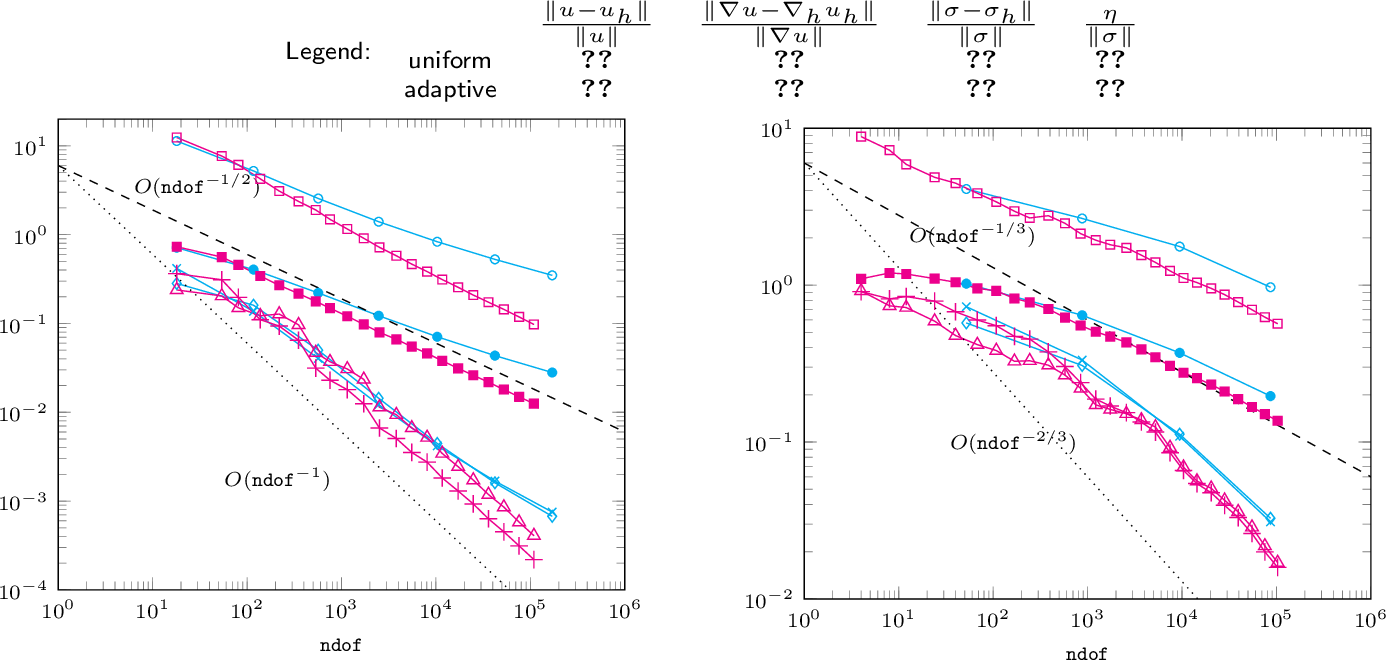
We solve the discrete biharmonic equation on sequences of uniform meshes as well as adaptive meshes based on the error estimator and Dörfler marking [40] with bulk parameter 1/3. 2 (left) displays the convergence history in this two-dimensional example. All displayed errors are relative errors. The symbol \(\mathtt{ndof}\) refers to the number of degrees of freedom. For illustrating the performance of the three-dimensional generalization of DKT, we consider the cylinder \(\Omega_3\mathrel{\vcenter{:}}=\Omega_2\times (0,1)\) and the tensor-product solution \(u_3(x,y,z) \mathrel{\vcenter{:}}= u_2(x,y) (z-z^2)^2\). 2 (right) displays the convergence history on uniform and adaptive meshes. In both experiments, uniform mesh-refinement leads to convergence in the \(\sigma\) variable with the asymptotic rate dictated by the singularity exponent of the exact solution, and higher rates for weaker norms. We observe that adaptive mesh refinement leads to the optimal rates \(1/n\) with respect to the number of degrees of freedom for the error in the \(\sigma\) variable. The errors in the weaker norms converge at the doubled rate. We observe efficiency indices \(\eta/\|\sigma-\sigma_h\|\) of around 10.

8 Conclusive remarks↩︎

The error analysis of this work can be applied to several other, classical nonconforming FEM that satisfy (C1)–(C5). They include but are not limited to the following examples: The Morley element [36], [41]; Fraeijs de Veubeke’s elements of type I and II [34], [42], the Specht element [43] and its generalization to higher space dimensions by [44], called New Zienkiewicz Triangle (NZT) therein; the Nilssen–Tai–Winther [23]. For these, (C1)–(C2) follow from the degrees of freedom, while (C3)–(C4) are trivial because \(\nabla_h = \nabla_\mathrm{pw}\). Since quadratic polynomials are subset of the local trial spaces, the construction of an interpolation operator satisfying (C5) can follow the proof outlined in 5. The trial functions of Specht and NTW elements are continuous, leading to convergence rates for the singular perturbation problem as in 3.

References↩︎