Decodable Is Not Grounded:
A Vision-Ablation Arbiter for VLM Spatial Reasoning
June 30, 2026
Abstract
The standard way to read latent knowledge out of a model, a linear probe confirmed by a steering recovery, can systematically overstate what a vision–language model (VLM) actually grounds in the image. We show this on spatial reasoning, where the error is invisible to both probing and steering yet exposed by a one-line causal control: replacing the image with a gray blank. Probes decode the within-axis answer at \(73\)–\(97\%\) across axes, and a training-free projection lifts a near-chance axis from \(59\%\) to \(79\%\), exactly the signature of unlocking latent knowledge. The blank-image arbiter refutes it, revealing three grounding regimes that probing conflates: an axis can be grounded (vision-dependent, correct), a prior (vision-independent, with its decode and its apparent recovery a directional default rather than perception), or, surprisingly, inverted: decodable, causally controllable, but deployed with the wrong sign, so the model scores below chance and the error requires looking. The taxonomy holds across the studied VLMs: in fourteen models spanning six language-model families and \(2\)B–\(27\)B, horizontal is grounded, vertical is a prior, and depth is inverted, with the inversion emerging at scale within families. The decode\(\neq\)deploy inversion replicates on seven of eight models across five families, and the minimal edit that re-deploys it varies with geometry: a training-free rotation matches a trained edit on the cleanest model, while distributed inversions need a trained low-rank edit, tracing a per-model correction-complexity spectrum. The cheap, self-calibrating arbiter cleanly separates grounded perception, inverted perception, and prior substitution; we argue it should be a default control for latent-knowledge and steering claims in VLMs.
1 Introduction↩︎
A vision–language model (VLM) can answer a spatial question below chance, and blinding it (replacing the image with a same-size gray blank) makes it more accurate: the model is not failing to use the image, it is using it backwards. This sits inside a more familiar pattern. A linear probe reads a target attribute out of activations even when the model answers questions about it poorly [@gurnee2024space; @linearspatiotemporal2026; @seeingbutnotbelieving2025], and the standard reading is that the model represents the attribute but fails to deploy it, motivating training-free interventions (steering, projection, representation engineering) that unlock the latent capability without gradient updates [@rimsky2024caa; @zou2023representation; @linearspatiotemporal2026]. This paper is a cautionary study of that inference: we follow the recipe to its natural conclusion on one model, Qwen2.5-VL-7B [@qwen2vl], and one controlled axis (egocentric directional judgement on ViewSpatial-Bench [@viewspatial2025]), then show the conclusion is wrong and that the corrected picture holds across fourteen models and six LM families (§5).
The seductive result. Camera-relative direction decomposes into horizontal (left/right), vertical (above/below), and depth (front/back). The model is strong on horizontal, near chance on vertical, and below chance on depth (§4), yet a linear probe decodes all three axes from the residual stream, vertical the most (\(94\%\) vs.horizontal’s \(85\%\)). A training-free projection along the vertical direction then lifts vertical accuracy from \(59\%\) to \(79\%\) while leaving horizontal untouched (§4.1), precisely the result one would publish as latent spatial knowledge recovered without training.
The arbiter. We then ask what the probe-and-steer pipeline never asks: does the recovered behavior depend on the image? A one-line control (replace the image with a same-size gray blank, leaving question and options unchanged; Fig. 1) fractures the single not-deployed story into three grounding regimes. Horizontal is grounded and correct (accuracy collapses \(82\%\to49\%\) when blinded). Depth is grounded and inverted (below chance with the image, \(31\%\); reverts to chance without it, \(45\%\), so the error requires looking). Vertical is not grounded: real and blank accuracy are identical (\(59\%\approx60\%\)), and the projection recovery gains the same with no image (\(+19\) blind vs.\(+21\) sighted), so the \(94\%\) decode reads a directional default-to-above prior, not vision.
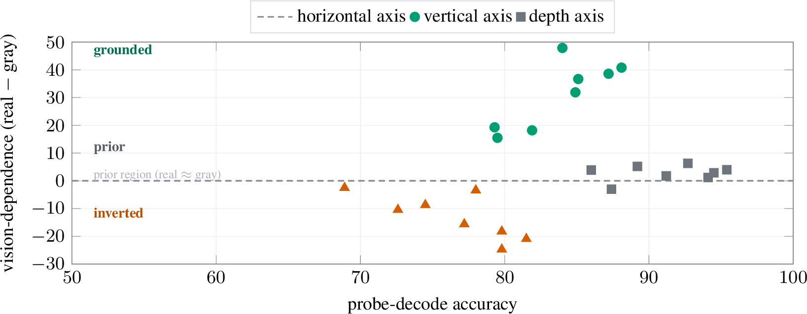
Why this matters. Vertical is the cautionary case: the most decodable axis, the cleanest training-free recovery, and the one axis that does not use vision, exactly the headline a decode-and-steer pipeline would report. Depth is the surprise: a model that scores below chance because it reads a real visual cue with the wrong sign. The vision-ablation arbiter catches both, is essentially free (one forward pass with pixels zeroed), and is discriminating rather than deflationary. Our contributions: (i) a three-regime grounding taxonomy (grounded-correct, grounded-inverted, prior-driven) and the finding that linear decodability and behavioral accuracy each fail to identify which regime an axis is in, the most decodable and most recoverable axis being the least grounded (§4–4.2); (ii) a cheap, discriminating vision-ablation arbiter, robust across five ablations including a real-but-mismatched in-distribution image, which we argue should be a default control for latent-knowledge and steering claims in VLMs (§4.2, §7); (iii) architecture-generality and a task-type boundary across fourteen VLMs, six LM families, and \(2\)B–\(27\)B: across capable models horizontal is grounded, vertical a prior, depth inverted (emerging with scale within families), and the same models that invert camera-egocentric depth are grounded-correct on near-field and metric depth (§5–5.1); and (iv) a correction that reads out the geometry: the inversion replicates on seven of eight models across five families, and the minimal re-deploying edit (training-free rotation on the cleanest model, matching a trained edit; a trained low-rank edit on distributed ones) traces a per-model correction-complexity spectrum (§6).
2 Related Work↩︎
Spatial reasoning in VLMs. Early benchmarks test two-object relations from canonical viewpoints (What’sUp [@kamath2023whatsup], VSR [@liu2023vsr]), now largely saturated [@cai2024spatialbot; @du2024embspatial]; the frontier targets egocentric and multi-perspective settings: VSI-Bench [@yang2024thinking], MMSI-Bench [@yang2025mmsi], OmniSpatial [@omnispatial2026], and ViewSpatial-Bench [@viewspatial2025], the source of our task. A large training-based literature closes these gaps with synthetic 3D supervision or RL [@chen2024spatialvlm; @spatialssrl2025; @daxberger2025mmspatial]; our study is diagnostic and training-free, orthogonal to those remedies.
Linear probing, spatial IDs, and probe validity. Linear world models for space have been read out of LLMs [@gurnee2024space; @linearspatialworld2025] and VLMs; most relevantly, [@linearspatiotemporal2026] identify linear spatial IDs that are causally steerable across VLMs. This establishes that spatial structure is linearly tractable and steerable; we ask the complementary question, whether a decodable, steerable direction is the one the model uses to look, and find the most decodable axis is the one that ignores the image. This connects to a long-standing caution: high decoding accuracy certifies linear presence, not use, and control tasks are needed to calibrate it [@hewitt2019control; @belinkov2022probing]. We provide a behavioral, causal control (vision ablation) rather than a probe-side one.
Latent spatial knowledge: present, but used how? A fast-growing line argues VLMs do represent space and that failures are an access problem. Closest to us, [@scenetopology2026] show a latent 3D-topology map exists but is overshadowed by semantics and surface it with a subspace + Dirichlet regularizer; [@beyondsemantics2025] blame vision-token norms suppressing positional cues and restore it by normalizing norms; [@geomfailures2026] explain multi-object errors as concept-vector interference and validate by steering; and concurrently [@whyfarup2026] find a vertical–distance entanglement that strengthens with scale. These share a template (locate a representation that is absent, overshadowed, entangled, or steerable, then surface or steer it) and assume the obstacle is access. Our phenomenon differs in kind: depth is present, correctly decodable, and causally controllable yet deployed with the wrong sign (decode\(\neq\)deploy), while vertical is decodable but behaviorally a prior. Our discriminator is a behavioral vision-ablation arbiter, and our remedy is a measured correction-complexity spectrum. A capability matrix (Appendix [app:additional], Table ¿tbl:tab:related?) places these works on common axes; the inversion regime and the cross-model correction ladder are, to our knowledge, unique here.
Steering and the actionability gap. Contrastive activation addition [@rimsky2024caa; @panickssery2024] and representation engineering [@zou2023representation], following the activation-editing tradition [@meng2022rome; @wang2023interpretability], inject a direction to change behavior. [@basu2026interp] give a pointed negative result: probes reach near-perfect AUROC while interventions correct only \(\sim\)20% of errors. We sharpen this from another angle: an intervention that moves accuracy can still act on a non-visual prior, so a behavioral success is not grounded recovery without a causal control. Relatedly, the VQA literature showed models exploit question priors and score well without the image [@goyal2017vqa; @agrawal2018dontassume]. Our arbiter shares that intuition but is applied per axis and reads the signed real\(-\)ablated difference, so it separates not just grounded from ungrounded but a regime a whole-question blind baseline cannot express: an inverted axis, image-driven yet deployed wrong-sign (below chance with the image, at chance without). [@seeingbutnotbelieving2025] document a related attention–correctness disconnect on spatial QA.
3 Setup↩︎
Task and axes. Our probe is one controlled task that cleanly separates three spatial axes. We use the Camera-Relative-Direction split of ViewSpatial-Bench [@viewspatial2025]: egocentric four-option questions “where is \(X\) relative to \(Y\) from the camera’s perspective” (\(1773\) items). We decompose each item by the physical axis its gold answer lies on (horizontal left/right, vertical above/below, depth front/back, and composite, diagnostic only) and run all causal experiments on the \(1047\) pure-axis items (per-axis counts in Table 2). We report native 18-way accuracy (chance \(25\%\)) and a binary within-axis accuracy (the two poles, order randomized; chance \(50\%\)), balanced wherever a pole split is skewed. The anchor is Qwen2.5-VL-7B-Instruct [@qwen2vl]; implementation details are in Appendix [app:additional].
Probing, steering, and the arbiter. For decodability we fit a five-fold CV logistic probe (PCA-50) on the decision-token residual stream per axis and layer, reporting accuracy over a shuffled-label floor. For causal tests we extract a per-axis direction (diff-of-means or back-projected probe weight) and add it at the decision token scaled in residual-stream standard deviations; the training-free projection amplifies the localized direction over the top-\(k\) neurons in the L20–24 band with a single global scalar \(\gamma\) and no gradients or labels (details in Appendix [app:additional]). The vision-ablation arbiter re-evaluates any condition with the image replaced by a same-size gray blank, prompt and decoding unchanged, and classifies each axis by the signed real\(-\)gray gap: grounded if real exceeds gray and gray falls to chance, inverted if real is below chance and gray reverts toward it, and prior if real and gray coincide within bootstrap CIs. We apply it to both baseline accuracy and the projection gain, and guard against input-degeneracy with five ablations (gray, black, noise, patch-scramble, and a real-but-mismatched same-axis image) required to agree (§4.2). Intervention hyperparameters (\(\gamma\), \(\theta\), layer band, top-\(k\)) are chosen on validation and frozen for the reported test numbers.
Generality battery. The deep mechanism is characterized on the anchor; for generality we run an independent battery (per-axis behavior, arbiter, per-layer probe) on thirteen further VLMs spanning six LM families and 2B–27B (full roster in §5), with per-model decode-peak layers re-found. We further run the behavioral battery on two external benchmarks (What’sUp [@kamath2023whatsup], 3DSRBench [@ma20243dsrbench]) and a nine-method depth correction battery (§6).
4 The Decode\(\neq\)Deploy Dissociation and a Vision-Ablation Arbiter↩︎
Behavior: a single grounded axis. The native task accuracy is \(45.4\%\) on the full \(1773\) items, matching prior ViewSpatial numbers and validating our evaluation. Decomposed by axis (Table 2), the model is strong on horizontal (\(74.9\%\) 18-way, \(81.3\%\) binary), near chance on vertical (\(26.9\%\) / \(58.5\%\)), and below chance on depth (\(16.3\%\) / \(30.7\%\); binary depth is below chance at \(p<10^{-5}\), binomial). Controls rule out shortcuts (a same-dimension distractor tracks full accuracy; the composite class scores above chance only with a left/right component, \(52.1\%\) vs.\(9.2\%\); Appendix 9.6): the model is competent on horizontal and defaults elsewhere. Depth below chance on a randomized two-choice question rules out position bias and points to a systematic inversion, not a prompt-wording artifact: rephrasing front/back as closer/farther from the camera leaves accuracy below chance (Table 1).
| Phrasing | acc. | vs.ch. |
|---|---|---|
| “front / back” | 28.1 | \(-21.9\) |
| “closer / farther” | 32.7 | \(-17.3\) |
r0.47
5pt
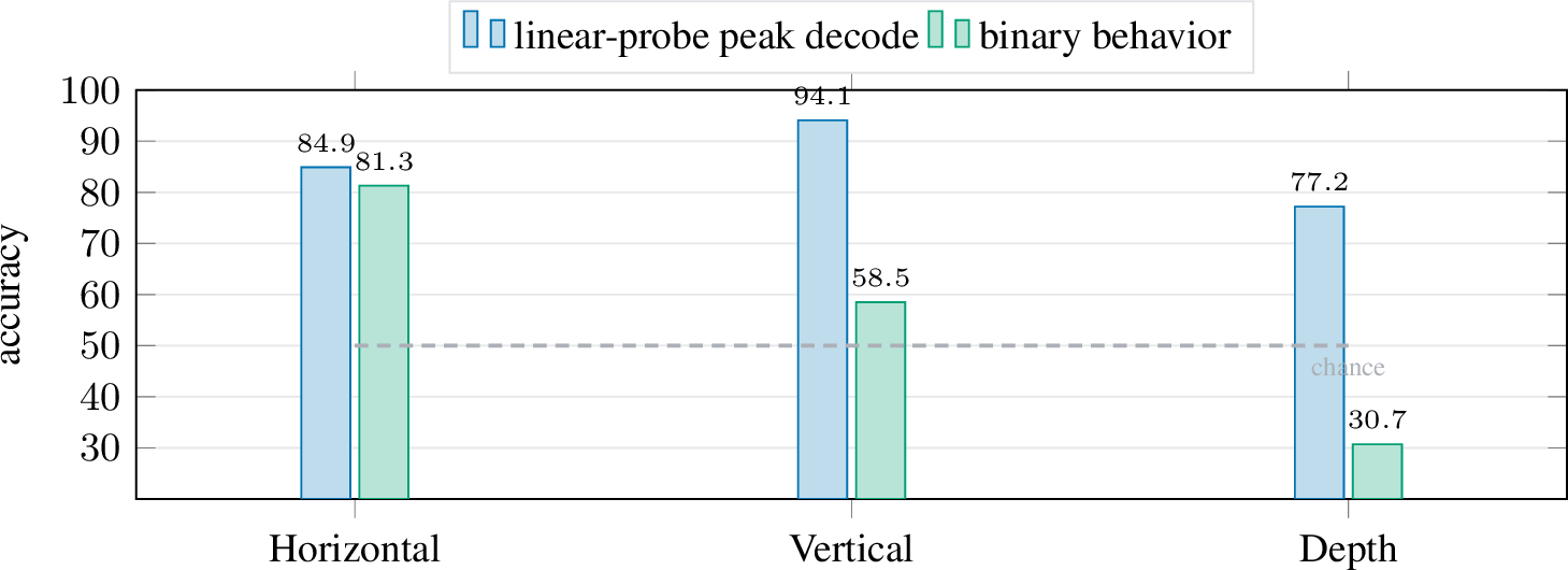
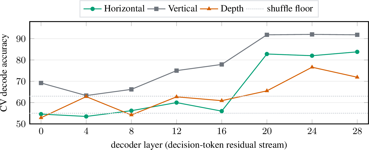
Decodability: every axis, vertical most. A linear probe tells a very different story (Fig. 7). Decoding the within-axis pole from the decision-token residual stream rises sharply at layers 16–24 for all three axes and peaks well above the shuffled-label floor: horizontal \(84.9\), depth \(77.2\), and vertical \(94.1\), the highest of the three. The image-pooled locus stays low everywhere (\(59\)–\(67\)), so the direction is assembled in the residual stream at the decision/text locus in mid-to-late layers rather than read directly off image tokens.
The dissociation. Placing behavior next to decodability (Table 2) gives the gap that drives the rest of the paper. Horizontal is decoded and deployed (gap \(+4\)). Vertical is the most decodable axis yet behaves near chance (gap \(+36\)). Depth is decodable while behavior runs below chance (gap \(+47\), anti-correlated). Taken on its own, this is the canonical knows-but-does-not-deploy picture: a strong latent representation (vertical \(94\%\)) that the model fails to act on, plus an inverted readout for depth. It is exactly the configuration that invites a training-free recovery method, which we build next.
| Axis | \(n\) | 18-way | binary | decode (shuffle) | gap | behavioral verdict |
|---|---|---|---|---|---|---|
| Horizontal (L/R) | 518 | 74.9 | 81.3 | 84.9 (57) | \(+4\) | deployed, correct |
| Vertical (up/dn) | 376 | 26.9 | 58.5 | 94.1 (63) | \(+36\) | near chance |
| Depth (front/back) | 153 | 16.3 | 30.7 | 77.2 (55) | \(+47\) | below chance |
5pt
4.1 An Intervention That Appears to Work↩︎
If vertical is decodable at \(94\%\) but behaves at chance, the natural move is to inject the decoded direction and watch behavior follow. It does.
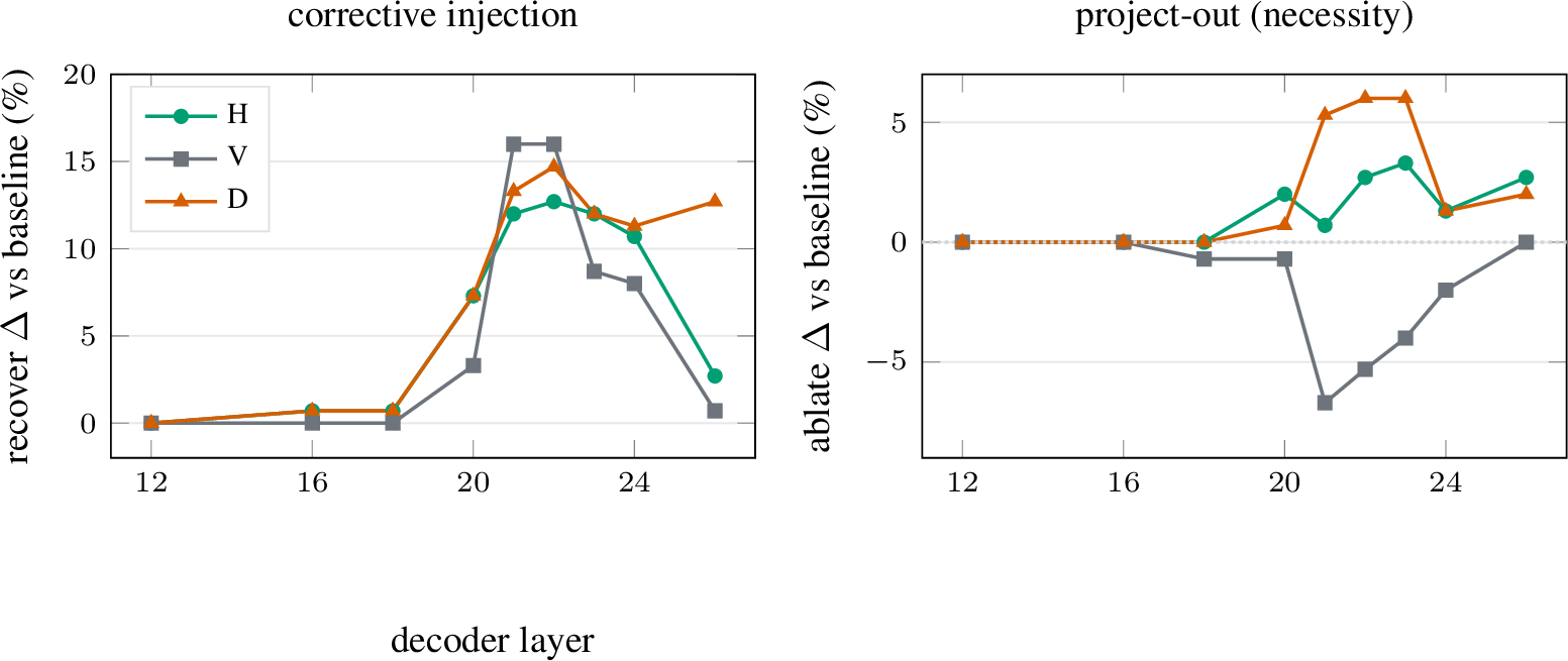
Causal steering. Adding the per-axis diff-of-means direction at the peak layer cleanly and monotonically moves the positive-pole probability for all three axes (Appendix 9.3, Fig. 11; depth moves the wrong way, confirming an inverted readout), establishing causal control. A corrective oracle raises vertical from \(59\%\) to \(74\%\), and projecting the direction out collapses it to chance, a necessity signature. A multi-layer band around the decode peak (L20–24) recovers far more than any single layer, locating the effect on a distributed path (Appendix 9.6, Table 10); the decoding-optimal probe direction is not the intervention-optimal one (Table 11).
Training-free projection. The strongest version uses no gradients or labels: we amplify the localized vertical signal with one global scalar \(\gamma\) (§3). Vertical rises from \(59\%\) to \(\mathbf{79\%}\) at \(\gamma{=}2\) (\(+21\)) with horizontal essentially unchanged (\(82\%\to81\%\)), positive across a broad range, while an off-band projection does nothing (Appendix 9.3, Fig. 2), so the lever is real and localized to the decode band. Depth does not lift cleanly, consistent with an inverted/entangled mode rather than an under-deployed one.
The result we could have stopped at. Vertical is the most decodable axis (\(94\%\)), behaves at chance (\(59\%\)), and is recovered to \(79\%\) by a training-free, label-free projection that leaves horizontal intact, while depth fails to recover, a clean dissociation. Reported as is, this reads as latent vertical spatial knowledge recovered without training. It would be wrong.
4.2 The Vision-Ablation Arbiter↩︎
The recovery in §4.1 never checked whether the behavior it moved depends on the image. We run that check by re-evaluating every condition with the image replaced by a same-size gray blank (§3). Numbers here are for Qwen2.5-VL-7B; §5 shows the regimes recur across fourteen models.
The arbiter is discriminating, not deflationary. The three axes respond to blinding in three predictable ways (Table 3). Horizontal collapses from \(82\%\) to chance (\(51\%\) balanced): its correct answers were image-driven, so the arbiter is a valid positive control. Depth sits below chance with the image (\(31\%\)) but rises to chance when blinded (\(45\%\)): the inversion itself is caused by the image; remove the input and the systematic error disappears. Vertical barely moves (\(59\%\to60\%\) raw, \(70\%\approx70\%\) balanced): the model is not using the image for vertical at all. Four further ablations (black, noise, patch-scramble, and a real but mismatched in-distribution image) give the same verdict (Appendix 9.6, Table 4), so the taxonomy is a property of how the model uses the image, not an artifact of the blank.
| baseline (raw) | baseline (balanced) | proj.gain | |||||
|---|---|---|---|---|---|---|---|
| 2-3(lr)4-5(lr)6-7 Axis | real | gray | real | gray | real | gray | grounding regime |
| Horizontal | 82.4 | 49.4 | 82.6 | 50.7 | \(+3\) | \(\sim\)0 | vision-dep.& correct |
| Depth | 31.4 | 45.1 | 31.6 | 46.3 | \(\le\)0 | \(\sim\)0 | vision-dep.& inverted |
| Vertical | 58.5 | 59.6 | 69.8 | 70.3 | \(+21\) | \(+19\) | vision-indep. (prior) |
5pt
Reading. Horizontal: removing the image collapses accuracy to chance (\(82\!\to\!49\)), and the projection gain vanishes with the gray image, so the signal is genuinely visual. Depth: real
accuracy is below chance but the gray image reverts to chance (\(31\!<\!45\)): the inversion is caused by looking at the image. Vertical: real \(\approx\) gray
under both raw and balanced scoring, and the projection gain is the same with or without the image, so the model is not using vision and the recovery amplifies a linguistic prior. Back-solving the per-class recalls on the \(31/69\) pole split gives recall\((\text{above})\!\approx\!99\), recall\((\text{below})\!\approx\!40\)
: a directional default-to-above response bias, not noise.
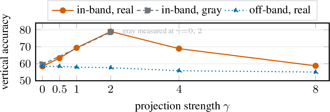
The recovery amplifies a prior. The decisive test is whether the projection gain of §4.1 needs the image. It does not: with the gray blank the vertical projection gains \(+19\) at \(\gamma{=}2\), indistinguishable from the \(+21\) it gains with the real image (balanced: \(+12\) blind vs.\(+14\) sighted). The lever is a direction that pushes the output distribution, and that distribution was never conditioned on the image. The horizontal control behaves oppositely: its small already-deployed gain vanishes under the blank, as there is no prior to amplify. What vertical encodes is a directional default: balanced accuracy (\(70\%\)) exceeds raw (\(59\%\)) on the \(31/69\) above/below split, with recall\((\text{above})\approx99\%\) and recall\((\text{below})\approx40\%\). The probe decodes vertical at \(94\%\) because this default-to-above is linearly readable, a language-side prior, the residual-stream analogue of a blind-VQA prior [@goyal2017vqa; @agrawal2018dontassume] that probe accuracy cannot distinguish from grounded knowledge [@hewitt2019control; @belinkov2022probing].
Consequence. The headline of §4.1 does not survive: vertical is a prior, not under-deployed visual knowledge, and depth is inverted rather than absent. Depth also resists a clean training-free flip: sweeping a signed projection at both signs, linear edits only neutralize the inversion toward chance (best \(\approx47\%\) vs.the \(\approx68\%\) a global sign-flip would give), revealing an entangled mode rather than a single free sign; a minimal trained edit at the causally localized layer does re-deploy it (§6). On this model, probing and steering overstate grounded spatial knowledge, and one cheap control says by how much and where.
| axis | real | gray | black | noise | scramble | mismatch | verdict |
|---|---|---|---|---|---|---|---|
| Horizontal | 82.6 | 50.7 | 49.6 | 47.4 | 54.1 | 50.7 | all \(\to\) chance (grounded, correct) |
| Vertical | 69.8 | 70.3 | 70.1 | 66.5 | 60.5 | 68.6 | all \(\approx\) real (prior) |
| Depth | 31.6 | 46.3 | 44.2 | 42.7 | 48.9 | 45.7 | all \(\to\) chance from below (inverted) |
6pt
The mismatch column is the decisive in-distribution control: a correct, real, same-axis image that simply does not match the question. Horizontal still collapses (\(50.7\)), vertical is unchanged (\(68.6\approx69.8\), so it ignores image content, not just image presence), and depth’s inversion relaxes to chance (\(45.7\)
). The taxonomy is not an artifact of feeding the model a degenerate blank.
5 The Taxonomy Is Architecture-General and Task-Specific↩︎
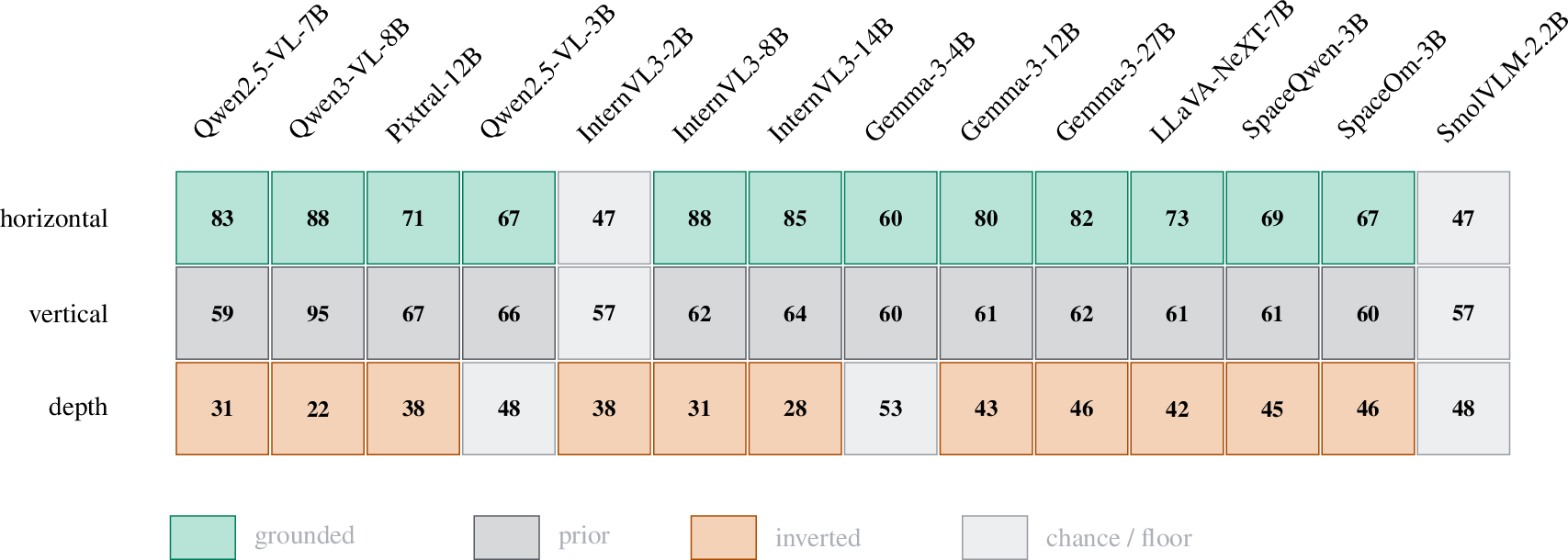
The single-model arc could be a Qwen2.5-VL-7B idiosyncrasy. We run the independent battery (per-axis behavior, the vision arbiter, and a per-layer probe) on thirteen further VLMs, for fourteen models across six LM families (Qwen2/2.5/3, Mistral, SmolLM, Gemma) and 2B–27B, including three within-family scale ladders (full roster in Appendix 9.4, Table 6; matrix in Fig. 3).
The three regimes recur across LM families. In every capable model horizontal is vision-dependent and correct (real \(\gg\) blank \(\to\) chance), vertical is prior-dominated (real \(\approx\) blank), and depth is at or below chance. This holds for Pixtral-12B (Mistral LM) and Gemma-3 (a different family with a SigLIP rather than Qwen-derived vision tower), so the taxonomy is a property of current VLMs, not a Qwen or InternViT artifact. SmolVLM-2.2B is the one all-axis exception, near chance even on horizontal (\(47\%\)): a capability floor below which no axis is grounded, exactly as expected.
Decodability overstates knowledge in every model. The probe decodes vertical at \(87\)–\(97\%\) and depth at \(73\)–\(86\%\) in every capable model while behavior on those axes is prior or inverted. This gap between what the probe reads and what the model grounds is systematic across architectures, and the cautionary claim of §4.2 is the paper’s most robust result.
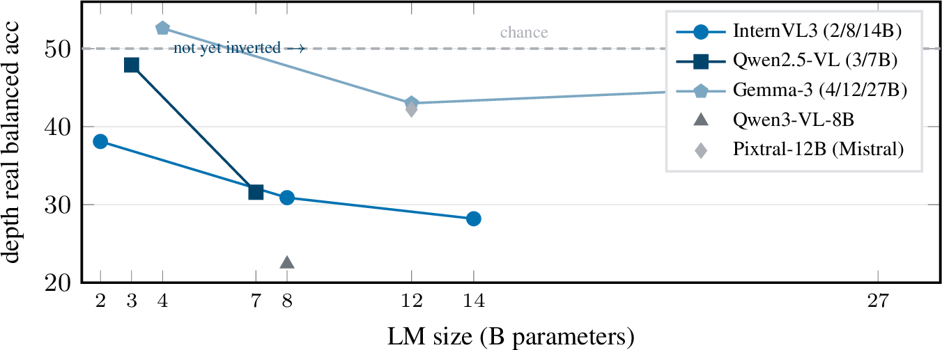
Depth inversion is scale-emergent within families. Three within-family ladders, varying only LM scale, show the inversion emerging with size (Appendix 9.4, Fig. 14): InternVL3 (\(38\%\to31\%\to28\%\)) and Qwen2.5-VL (\(48\%\to32\%\)) deepen monotonically, and in Gemma-3 (\(53\%\to43\%\to46\%\)) it emerges by 12B with horizontal grounding also emerging (\(50\%\to67\%\)). Onset and severity are family-modulated (InternVL3 is inverted already at 2B, Qwen2.5-VL-3B and Gemma-4B not yet, and Gemma-3 partially recovers at 27B), so the law is that inversion emerges with LM scale within a family, with degree and onset family-specific.
The LM backbone sets the fingerprint. LLaVA-OneVision-7B and InternVL3-8B share the Qwen2-7B LM with different vision towers (SigLIP vs.InternViT) and are qualitatively identical on all three axes, differing only in the magnitude of the weak vertical vision signal. The grounding fingerprint is thus driven by the language backbone with the vision tower and scale tuning the degree, consistent with the locus analysis (Appendix [app:layers], Fig. 7), where the axis signal is assembled LM-side.
5.1 External Benchmarks: A Task-Type Boundary↩︎
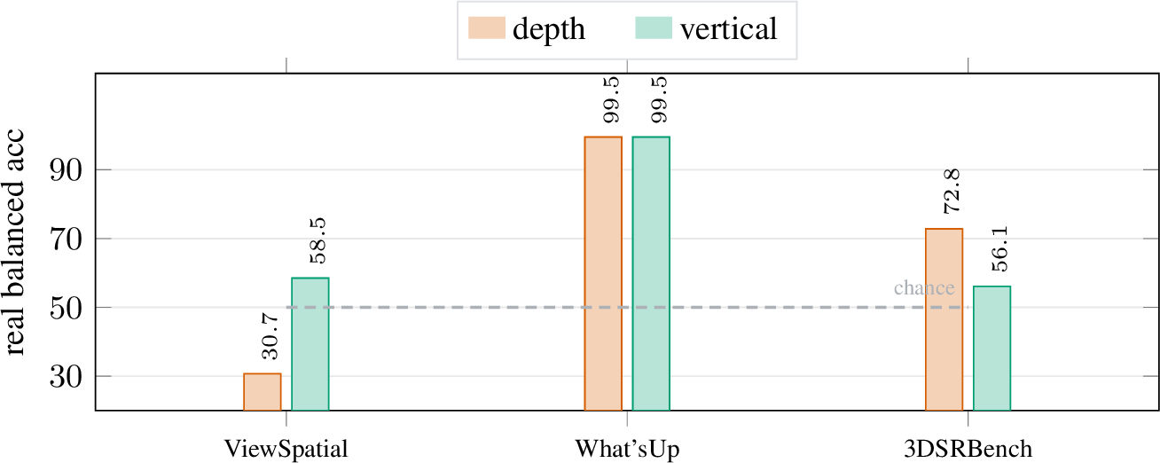
A single-benchmark taxonomy invites the objection that ViewSpatial is simply broken on the non-horizontal axes. We test this by running the behavioral battery and arbiter on two external benchmarks (What’sUp [@kamath2023whatsup], tabletop on/under and front/behind; and 3DSRBench [@ma20243dsrbench], real-scene height and closer-to-camera), mapping their categories onto our axes Table 5. The result replicates the taxonomy and sharpens it into a task-type boundary.
Depth inversion is camera-egocentric, not a general depth failure. The decisive result is a dissociation within the same model (Appendix 9.4, Table 5): Qwen2.5-VL-7B inverts depth on ViewSpatial’s camera-relative front/back yet is grounded-correct on What’sUp near-field front/behind and 3DSRBench closer-to-camera, with mismatch controls confirming both are vision-driven; four further models show the same pattern, and horizontal replicates cleanly everywhere as a positive control. The inversion is thus a reproducible property of camera-egocentric front/back framing, a task type rather than a missing capability or a benchmark artifact, which pre-empts the artifact objection by exhibiting the contrast in one model. Vertical is likewise task-type-dependent (grounded on tabletop on/under, a prior on ViewSpatial above/below and 3DSRBench height): grounding is organized by task type, with simple near-field contact relations grounded while abstract camera-perspective and real-scene relations fall back to priors or invert, and the arbiter transfers unchanged to make this legible.
6 Correcting the Inversion Diagnoses Its Geometry↩︎
If the depth axis is decodable and causally controllable (§4.1) but read out with the wrong sign, what is the minimal edit that re-deploys it? We run a battery of nine corrections (scalar recalibration, logit-lens reflection, a norm-preserving angular rotation [@angular2025], selective multi-layer rotation, activation edits SEA [@sea2024] and SADI [@sadi2024], per-head reflection ITI [@iti2023], SAE feature steering [@pach2025saevlm], and a trained low-rank edit LoRA [@lora2021] / ReFT [@wu2024reft]) on four models, then test generalization on four more (Appendix 9.5). Two findings emerge: the decode\(\neq\)deploy inversion is a population phenomenon, and the minimal correction is a per-model complexity spectrum.
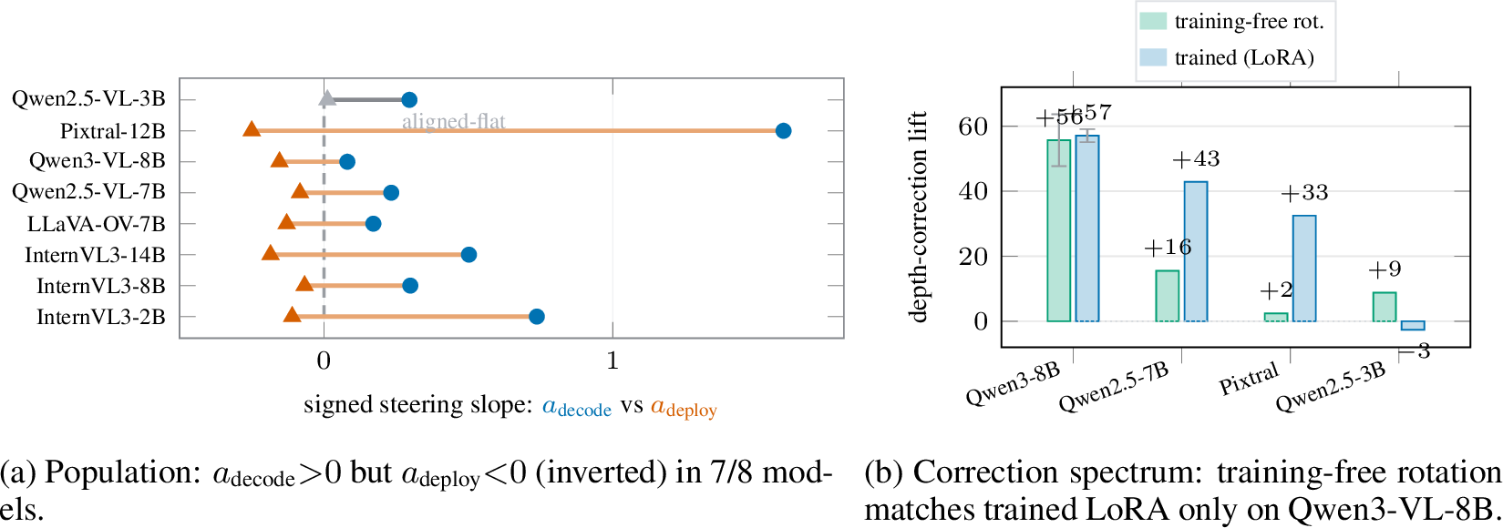
The inversion is a population phenomenon. A signed-slope diagnostic (the sign of the steering response of decodability versus behavior along depth) finds the inverted configuration (decode-slope \(>0\), deploy-slope \(<0\)) on seven of eight inverted-capable models across five LM families (Fig. [fig:forest], Table 8); the only exception is the not-yet-inverted scale floor Qwen2.5-VL-3B. Decodability rises with the steer everywhere while behavior moves the opposite way, ruling out a single-model artifact.
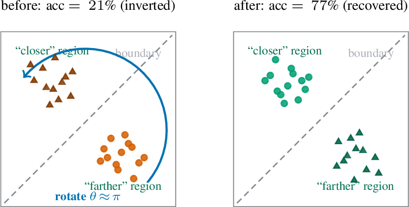
The minimal correction is a per-model complexity spectrum. Which correction re-deploys the axis reads out each model’s geometry. On Qwen3-VL-8B, the cleanest case, a training-free, norm-preserving rotation by \(\theta\approx\pi\) nearly triples depth accuracy (\(21\%\to77\%\)) and, across three seeds, matches a trained low-rank edit (\(+49{\pm}8\) vs. \(+55{\pm}2\)): the predicted un-inversion with no training. Across the population, which rung suffices is itself the diagnostic: a clean rotation on Qwen3-VL-8B, a partial one on LLaVA-OV (\(+14\)) and InternVL3-8B (\(+8\)), recalibration on InternVL3-14B, a trained edit on the distributed Qwen2.5-VL-7B (\(+43\)), and suppress-only (decodable but not installable) on InternVL3-2B and Pixtral-12B. The minimal sufficient correction ladders with the geometry (recalibration \(\to\) rotation \(\to\) trained low-rank \(\to\) none), and the winning rung is a per-model fingerprint (Fig. [fig:method]; full battery in Appendix 9.5, Table 7).
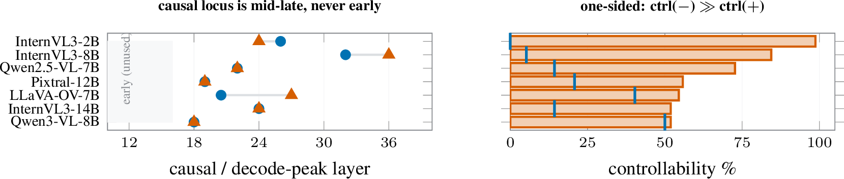
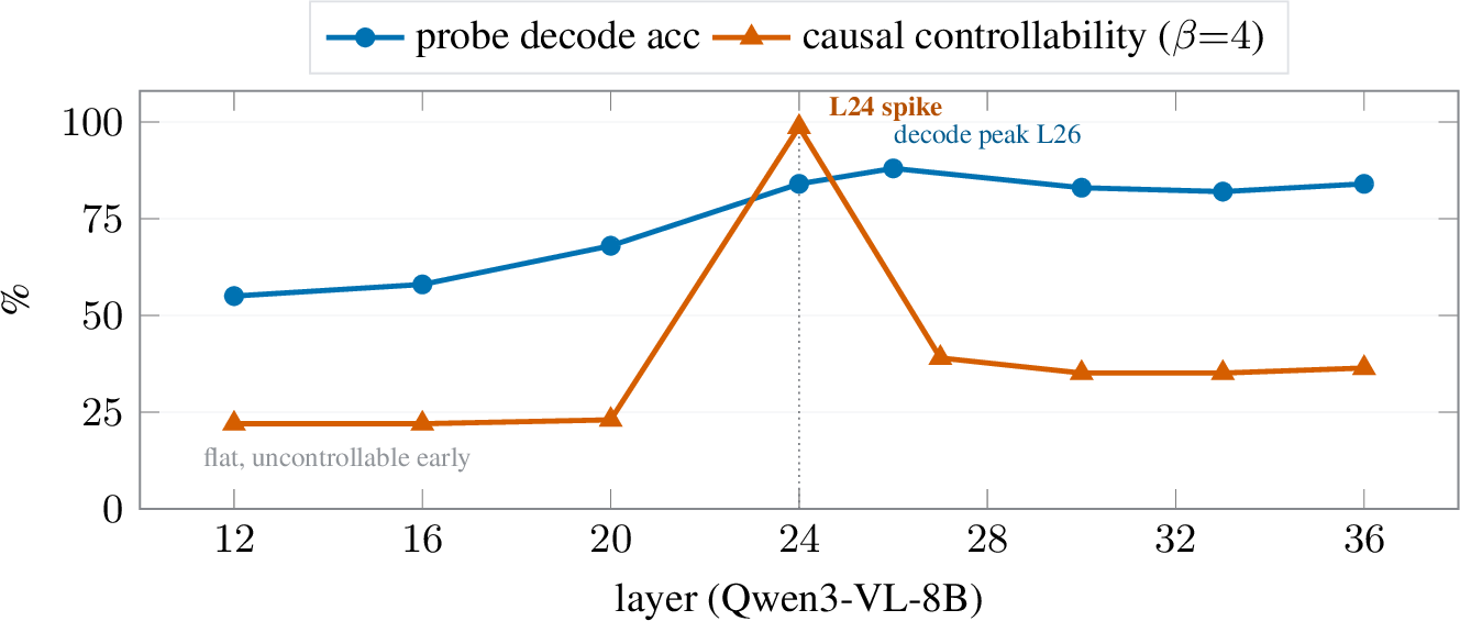
The causal locus is mid-late, one-sided, and shared across the population. Localizing the inverted channel layer-by-layer in seven models (Fig. 5), the causal-controllability peak sits mid-late (L19–36), at or downstream of the decode peak and never early, and is strongly asymmetric (one steer sign recovers correct depth, the opposite does almost nothing) in 6/7 models; its magnitude tracks correction-complexity (\(0.99\) for Qwen3-VL-8B down to \(\le0.56\) for trained-only models), so localization and correction cross-validate. On Qwen3-VL-8B (Appendix 9.5, Table 9) the correctable channel is low-dimensional yet off the probe axis (a rank-1 ReFT \(+58\) and a 4-component ICA reflection \(+60\) recover it; the single probe direction and a GEVD subspace fail, \(+0\)); the training-free\(=\)trained tie is seed-stable. This closes the arc from diagnosis through mechanism to a geometry-diagnostic correction: a shared inversion whose minimal fix, per model, reads out its geometry.
7 Discussion and Conclusion↩︎
Decodability is not grounding, and steering recovery is not either. Both halves of the standard latent-knowledge pipeline failed to flag the vertical prior: the probe called it the most present axis (\(94\%\)) and the projection the most recoverable, yet neither measures whether behavior is conditioned on the image, so their agreement is not corroboration. This sharpens the actionability-gap caution of [@basu2026interp]: a behavioral gain is not grounded recovery without a control.
The arbiter as a default control, and why three regimes. The vision ablation is cheap, assumption-light, and self-calibrating: it drives the genuinely visual horizontal axis to chance, so a null on another axis is informative rather than an input artifact. A two-way grounded-vs-not split would lump depth with the failures; the arbiter separates depth (vision-dependent, wrong sign) from vertical (vision-independent). We recommend reporting real-vs-ablated accuracy and treating a gain that survives ablation as prior amplification. Probing and steering overstate grounded knowledge because they are blind to image-dependence; the arbiter is not.
Why the inversion arises. Four convergent findings point to a learned frame-convention conflict rather than random damage. The inversion is construct-bound (grounded-correct on external depth, inverted only on ViewSpatial camera-relative front/back; Table 5), scale-emergent (deepens with LM scale, so learned), image-driven (not a fixed text prior; Appendix 9.6), and a geometric mis-rotation (a norm-preserving rotation re-deploys it). The convergence indicates a depth readout learned against ViewSpatial’s camera-relative convention; tracing it to training data is future work.
Limitations. Depth-inversion emerges with LM scale but not monotonically; SmolVLM-2.2B bounds the horizontal-universal claim to capable models; and our causal evidence is representation-level, as a clean pixel-level minimal pair for camera-relative front/back is unattainable (a mirror is identity for front/back, with no same-image pairs).
Reproducibility Statement↩︎
All experiments use publicly available open-weight VLMs and the public ViewSpatial-Bench, What’sUp, and 3DSRBench datasets. The task/axis decomposition, behavioral protocols (18-way and binary), probe (five-fold CV logistic on PCA-50 decision-token features with a shuffled-label floor), the training-free projection, the vision-ablation arbiter and its five image controls, the cross-model battery, and the nine-method correction battery are specified in §3 and Appendix [app:additional]; per-model layers, hyperparameters, seeds, and the multi-seed protocol for the rotation/trained-edit comparison are reported with the corresponding results (§6, Appendix 9.5). Limitations of single-seed and single-anchor analyses are stated explicitly in §7.
8 Implementation Details↩︎
8.0.0.1 Model and decoding.
Qwen2.5-VL-7B-Instruct [@qwen2vl], loaded in 4-bit nf4 on a single RTX 4090, attn_implementation="sdpa" (flash-attention not installed), greedy decoding, max_new_tokens=8. The
language tower has 28 decoder layers, hidden size 3584; the image token id is 151655. We index hidden_states[\(i\)] as the output of decoder layer \(i{-}1\). For
Qwen2.5-VL under transformers 4.57 the decoder path is model.model.language_model.layers; we use a multi-path fallback to remain robust to version changes.
8.0.0.2 Answer reading.
Letters are matched robustly over the variants "A"/" A" to avoid tokenization-induced baseline drift. In the binary protocol the positive-pole letter is randomized per item; all scoring, steering targets, and projections use
the per-item positive-pole map, and we verify the evaluation reproduces canonical baselines (V \(0.585\) / H \(0.824\) / D \(0.314\)) before trusting any
intervention number.
8.0.0.3 Probing.
Decision-token residual-stream activations are cached for all layers (\(L{=}29\) including the embedding, \(d{=}3584\)) over the \(1047\) pure-axis items. Per axis and layer we fit a five-fold cross-validated logistic regression on PCA-50 features; the shuffled-label probe gives the chance floor reported in brackets. We also report a light \(|d'|\) sparse-neuron localizer on decision-token activations; cross-axis top-20 neuron overlap is near zero, indicating distinct codes.
8.0.0.4 Steering scale.
Raw unit-vector steering (\(\alpha\hat{d}\), \(\alpha\le8\)) is negligible against residual-stream norms of \(170\)–\(245\) and produces null effects. We therefore scale by the standard deviation of the projection of activations onto \(\hat{d}_l\), so \(\alpha\) counts standard deviations; we cap \(|\alpha|\le4\) because larger values over-steer (at \(|\alpha|{=}6\) the injected norm reaches \(\sim\)65% of \(\lVert h\rVert\)). Causal-control claims rest on the monotonicity of \(P(+\text{pole})\), not on accuracy at extreme \(\alpha\).
8.0.0.5 Training-free projection.
On the \(k{=}64\) highest-\(|d'|\) neurons in the localized band we add \(\gamma\,(\sum_i \mathrm{sign}(d'_i)\,a_i(x))\,\hat{d}_l\) to the down-projection output, with a single global \(\gamma\) and no gradient updates. The band is L20–24 (vertical L21–25, depth L19–23); the off-band control uses L2–6. We note that \(\gamma\) is currently swept on the evaluation set; a held-out \(\gamma\) selection is the correct protocol and we report the broad positive range rather than a single value to mitigate this.
8.0.0.6 Arbiter.
The gray-blank image is constructed at the same resolution as the real image and passed through the identical preprocessing path (make_prompt_blank), so the only change is pixel content. Baseline and projection are re-evaluated under this
input with all else fixed.
9 Additional Results↩︎
5pt
@l *6c @ & & & & & &
Beyond Semantics [@beyondsemantics2025] & & & & & &
3D Scene Topology [@scenetopology2026] & & & & & &
Geometry of Failures [@geomfailures2026] & & & & & &
Why Far Looks Up [@whyfarup2026] & & & & & &
Spatial IDs [@linearspatiotemporal2026] & & & & & &
Actionability gap [@basu2026interp] & & & & & &
Ours & & & & & &
(behavioral): relate representation to behavior but not via a per-axis causal vision-ablation control.
(Ours, training-free): rotation is training-free on the clean-rotation model; distributed inversions still need a trained edit.
This appendix contains the supporting figures and tables referenced from the main text: the layer-wise analyses (§[app:layers]), the full cross-model and external-benchmark results (§9.4), the complete correction battery and population mechanism (§9.5), and robustness controls (§9.6).
9.1 The dissociation, in detail↩︎
Figure 6 plots behavior against decodability for the anchor model, the visual form of the main-text Table 2.
9.2 Layer-wise analyses↩︎
| benchmark | axis (task) | real | gray | mismatch | verdict |
|---|---|---|---|---|---|
| Qwen2.5-VL-7B anchor | |||||
| What’sUp-A | horizontal (left/right) | 99 | 51.5 | 51.5 | grounded |
| What’sUp-A | vertical (on/under) | 99.5 | — | 47.6 | grounded |
| What’sUp-B | horizontal | 100 | — | 47.1 | grounded |
| What’sUp-B | depth (front/behind) | 99.5 | 50 | 48.5 | grounded-correct |
| 3DSRBench | vertical (height) | 56.1 | 56.2 | 54.1 | prior |
| 3DSRBench | depth (closer-to-cam) | 72.8 | 56.6 | 49.4 | grounded-correct |
6pt
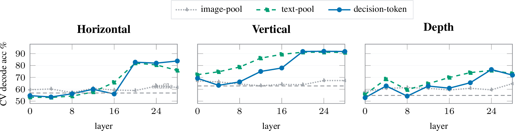
Complementing the main-text locus figure (Fig. 7), the per-layer decision-token decode peaks at L20–24 (Fig. 8), and the causal locus coincides with this decode onset (Fig. 9). On the second model, the inverted depth channel is causal, sharply localized, and one-sided across the population (Fig. 5), with a layer-wise decode/controllability profile shown in Fig. 10.
9.3 Intervention geometry↩︎
The causal sweep (Fig. 11) and the diff-of-means projection (Fig. 2) establish causal control; the un-inversion is a near-\(\pi\) rotation of the readout (Fig. 12).

9.4 Full cross-model and external results↩︎
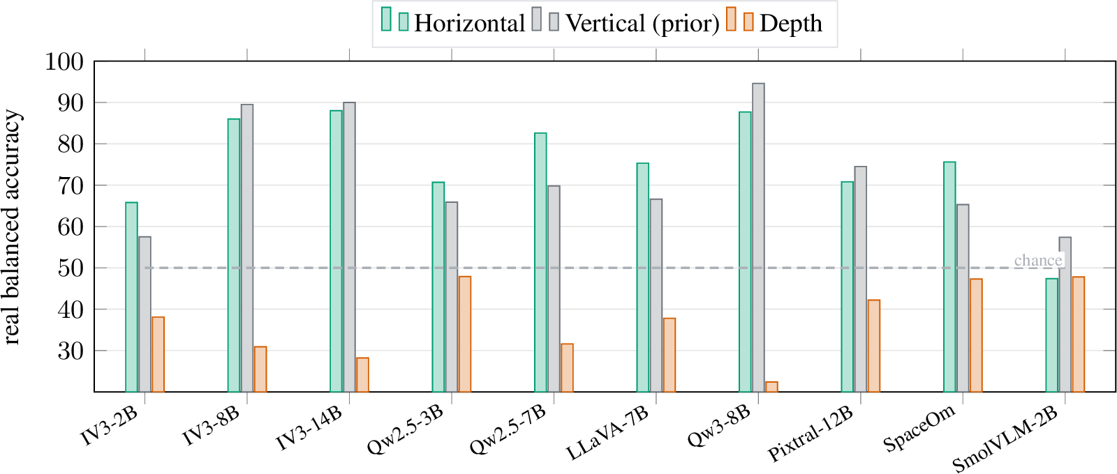
Table 6 is the complete fourteen-model roster behind the matrix figure (Fig. 3); Fig. 13 summarizes per-axis behavior and Fig. 14 the within-family scale ladders. On external benchmarks the inversion becomes a task-type boundary (Fig. 15, Table 5): the same models that invert ViewSpatial camera-egocentric front/back are grounded-correct on near-field front/behind and metric closer-to-camera depth.
| model | LM family | H | V | D | note |
|---|---|---|---|---|---|
| InternVL3-2B [@internvl3] | Qwen2-based | 65.8 | 57.5 | 38.1 | ladder: already inverted at 2B |
| InternVL3-8B | Qwen2-7B | 86 | 89.5 | 30.9 | ladder (monotone) |
| InternVL3-14B | Qwen2.5-14B | 88 | 90 | 28.2 | ladder: deepest |
| Gemma-3-4B [@gemma3] | Gemma/SigLIP | 49.5 | — | 52.6 | ladder: H & D not yet (small) |
| Gemma-3-12B | Gemma/SigLIP | 67.3 | 75.9 | 43 | ladder: deepest |
| Gemma-3-27B | Gemma/SigLIP | 69.8 | 78.4 | 45.6 | ladder: partial recovery (non-mono.) |
| Qwen2.5-VL-3B [@qwen2vl] | Qwen2.5 | 70.7 | 65.9 | 47.9 | depth not yet inverted |
| Qwen2.5-VL-7B | Qwen2.5 | 82.6 | 69.8 | 31.6 | primary (deep mechanism) |
| LLaVA-OV-7B [@llava_onevision] | Qwen2-7B | 75.3 | 66.6 | 37.8 | \(\approx\) InternVL3-8B (shared LM) |
| Qwen3-VL-8B [@qwen3vl] | Qwen3 | 87.7 | 94.6 | 22.4 | newest; most inverted |
| Pixtral-12B [@pixtral2024] | Mistral | 70.8 | 74.5 | 42.2 | non-Qwen; taxonomy holds |
| SpaceOm [@spacevlms] | Qwen2.5 (sp-FT) | 75.6 | 65.3 | 47.3 | spatial-FT did not fix V/D\(^{\dagger}\) |
| SpaceQwen-3B [@spacevlms] | Qwen2.5 (sp-FT) | 50.2 | 56.2 | 49.9 | near-chance; not a donor\(^{\dagger}\) |
| SmolVLM-2.2B [@smolvlm2025] | SmolLM | 47.4 | 57.4 | 47.8 | capability floor (even H \(\approx\) chance) |
5pt
Shaded = within-family scale ladders (InternVL3 and Qwen2.5 monotone; Gemma non-monotone, 27B partially recovers; Fig. [fig:depth95scale]). \(^{\dagger}\)
The two spatial-fine-tuned models (SpaceOm, SpaceQwen) are grounded-correct on no failing axis, so neither is a clean “donor”; SpaceOm is a thinking model whose first-token eval likely understates it. SmolVLM-2.2B is near-chance on all axes, bounding “horizontal universal” to capable models.
9.5 Correction battery, population, and second-model mechanism↩︎
Table 7 is the full nine-correction battery behind the main-text Fig. [fig:method]; Table 8 is the eight-model population behind the main-text forest plot (Fig. [fig:forest]); Table 9 reproduces the deep mechanism on a second model.
| correction | qwen-7B | qwen3-vl-8B | pixtral-12B | 3B |
|---|---|---|---|---|
| recalibrate (\(1\)-D scalar) | \(+11.2\) | \(+0\) | \(+1\) | \(+0\) |
| logit-lens reflect-at-onset | n/a | \(+0\) | \(+0.7\) | \(-2.7\) |
| angular rotate (\(\theta{\approx}\pi\)) [@angular2025] | \(+8.8\) | \(\mathbf{+55.7}\) | \(+0.7\) | \(+8.8\) |
| selective multi-layer rotate [@angular2025] | \(+15.5\) | \(\mathbf{+54.8}\) | \(+2.4\) | \(+1.9\) |
| SEA [@sea2024] / SADI [@sadi2024] edits | \(+10\) | \(+6\) | \(+1\) | \(+1.4\) |
| ITI per-head reflect [@iti2023] | \(+5.5\) | \(+1.4\) | \(+0\) | \(+0.2\) |
| SAE feature steer\(^{\ddagger}\) [@pach2025saevlm] | \(+2.9\) | \(+1.2\) | \(+0.2\) | \(-1.2\) |
| LoRA [@lora2021] / ReFT [@wu2024reft] (trained) | \(\mathbf{+42.9}\) | \(\mathbf{+57.1}\) | \(\mathbf{+32.5}\) | \(-2.6\) |
| card-C rung | reflect (1-D) | rotate (2-D) | none (trained) | none (not inv.) |
| inversion geometry | distributed | clean rotation | not-installable | flat (not inv.) |
6pt
Shaded: training-free rotation wins, trained edit needed. On Qwen3-VL-8B the training-free rotation (\(+55.7\), \(21.4\!\to\!77.1\), test \(>\) val: not overfit) matches trained LoRA (\(+57.1\)). \(^{\ddagger}\)The SAE feature diagnostic
is exploratory and is not used as evidence. The training-free\(\approx\)trained match on Qwen3-VL-8B holds over three seeds (§[sec:sec:method]), and the population picture is the decode\(\neq\)deploy forest of §[sec:sec:method]. The card-C rung is the minimal-complexity fixed correction within margin of the best lift (a per-model effective-dimensionality fingerprint); the four models shown are clear cases; borderline
models (e.g.
InternVL3-8B/14B) are reported separately.
| model | family | base | \(a_{\text{dec}}\) | \(a_{\text{dep}}\) | rotate\(^{*}\) | recalib | correctability |
|---|---|---|---|---|---|---|---|
| InternVL3-2B [@internvl3] | InternVL3 | 38.3 | \(+.74\) | \(-.11\) | \(-2.1\) | \(+1.4\) | suppress-only |
| InternVL3-8B | InternVL3 | 26.4 | \(+.30\) | \(-.07\) | \(+8.1\) | \(+2.6\) | mild rotation |
| InternVL3-14B | InternVL3 | 31.4 | \(+.50\) | \(-.19\) | \(-1.0\) | \(\mathbf{+6.2}\) | recalib/reflect |
| LLaVA-OV-7B [@llava_onevision] | LLaVA | 36.2 | \(+.17\) | \(-.13\) | \(\mathbf{+13.8}\) | \(+7.9\) | moderate rotation |
| Qwen3-VL-8B | Qwen3 | 21.4 | \(+.08\) | \(-.15\) | \(\mathbf{+55.7}\) | \(+6.0\) | clean rotation \(=\) trained |
| Qwen2.5-VL-7B | Qwen2.5 | 26.2 | \(+.23\) | \(-.08\) | \(+15.5\) | \(+11.2\) | distributed (trained) |
| Pixtral-12B [@pixtral2024] | Mistral | 39.8 | \(+1.59\) | \(-.25\) | \(+2.4\) | \(+1.0\) | not-installable (trained) |
| Qwen2.5-VL-3B [@qwen2vl] | Qwen2.5 | 48.1 | \(+.30\) | \(+.01\) | \(+8.8\) | \(+0.0\) | aligned-flat (not inverted) |
5pt
\(a_{\text{dec}}/a_{\text{dep}}\): signed steering slopes for probe-decodability and behaviour (both \(>0\) in the only non-inverted model). 7 of 8 models across 5 families are
inverted; only the 3B scale-floor is not. rotate\(^{*}\)
is the best norm-preserving angular rotation (training-free); recalib is the best 1-D scalar grid lift.
| correction | best setting | test | lift | reading |
|---|---|---|---|---|
| ReFT [@wu2024reft] (trained) | rank 1, L30 | \(\mathbf{79.2}\) | \(\mathbf{+57.8}\) | low-rank trainable (val\({\approx}\)test) |
| ICA-subspace reflect | \(k{=}4\), L30 | \(\mathbf{81.0}\) | \(\mathbf{+59.5}\) | multi-component, off probe axis |
| probe-direction reflect | \(k{=}1{\dots}8\) | \(21.4\) | \(+0.0\) | single probe axis fails |
| GEVD subspace (closed-form) | \(k{=}1\), L30 | \(21.7\) | \(+0.2\) | closed-form basis fails |
6pt
The trained ReFT lift (\(+57.8\)) matches this model’s correction-battery LoRA (\(+57.1\), Table [tbl:tab:method], LoRA [@lora2021]). That ICA (\(k{=}4\)) succeeds where the single probe direction does not echoes the cheap-lens
vs.
probe contrast and locates the readout error in a small, non-probe-aligned subspace.
9.6 Robustness controls and auxiliary analyses↩︎
| Axis | band | baseline | recover | ablate | reading |
|---|---|---|---|---|---|
| Horizontal | L19–23 | 82.4 | 98.1 (\(+15.6\)) | 82.2 (\(-0.2\)) | deployed; ablate flat (redundant) |
| Vertical | L21–25 | 58.5 | 70.2 (\(+11.7\)) | 49.2 (\(-9.3\)) | recoverable & necessary (ablate\(\to\)chance) |
| Depth | L19–23 | 31.4 | 62.7 (\(+31.4\)) | 36.6 (\(+5.2\)) | sign-flip crosses chance; ablate helps |
6pt
Recover uses a GT-signed corrective injection: it shows the direction is causally usable, not that test accuracy improves. The arbiter (Table [tbl:tab:arbiter]
) shows the vertical lever operates on a prior rather than on vision.
| Axis | direction | bias range | oracle | ablate (rand) |
|---|---|---|---|---|
| Horizontal | diff-of-means | \(0.29\!\to\!0.72\) | 0.950 | 0.820 (0.824) |
| probe | \(47\!\to\!57\) | 87.8 | 82.8 (82.4) | |
| Vertical | diff-of-means | \(0.55\!\to\!0.85\) | 0.739 | 0.500 (0.586) |
| probe | \(64\!\to\!77\) | 65.4 | 57.7 (58.6) | |
| Depth | diff-of-means | \(0.57\!\to\!0.28\) | 0.464 | 0.366 (0.314) |
| probe | \(48\!\to\!43\) | 34.6 | 31.4 (31.4) |
6pt
| model | depth acc | prior bias | align-on-err | verdict |
|---|---|---|---|---|
| Qwen2.5-VL-7B [@qwen2vl] | 32.7 | 45.1 | 66.0 | not-prior-dominated |
| Qwen3-VL-8B [@qwen3vl] | 23.5 | 8.5 | 62.4 | not-prior-dominated |
| Pixtral-12B [@pixtral2024] | 41.2 | 8.5 | 71.1 | not-prior-dominated |
7pt
The verdict is driven by the model-specific below-chance accuracy (which differs across models, \(23.5\)–\(41.2\)), so it is robust; we do not rely on the precise prior-bias magnitudes (the
blank-image eval reported a suspiciously identical bias for two models and is flagged for re-verification). This establishes a negative
answer to “why” (not a prior); a positive egocentric-vs-allocentric frame-flip test is left to future work.
9.6.0.1 Why does it invert? A negative answer (not a prior).
Replacing the image with a blank/gray input and measuring the lopsidedness of the answer (Table 12) rules out the simplest explanation—a fixed text-convention prior (“front means farther”). A pure prior would floor depth accuracy at chance, but all three clearly-inverted models score below chance with the real image, which a mild blank-image bias cannot produce. The inversion is therefore image-driven: the model perceives the depth cue and deploys it with a flipped sign. This is a negative “why”; a positive egocentric-vs-allocentric frame-flip account is left to future work.
9.6.0.2 Composite class and the L/R crutch.
The composite class (\(n{=}726\)) scores \(39.9\%\) overall, but split by whether the gold answer carries a left/right component it is \(52.1\%\) (with L/R, \(n{=}520\)) vs.\(9.2\%\) (without L/R, \(n{=}206\)). A confusion analysis shows horizontal stays on-axis (\(79\%\)) while vertical and depth escape to composite (\(45.7\%\) / \(49.7\%\)), coherent with horizontal carrying the only grounded directional signal.
10 Negative Results and a Methodological Note↩︎
10.0.0.1 A masked-LoRA tuning ladder that we discarded.
Before the training-free projection we ran a neuron-targeted masked-LoRA fine-tune (300 steps) on the vertical axis, comparing \(d'\)-localized neurons against random in-band neurons and against tuning the whole band. The \(d'\)-localized run recovered vertical strongly while preserving horizontal, which looked like evidence that the localized neurons specifically “deploy” vertical. We do not report it as a result for two reasons. First, a random-in-band control recovered vertical almost identically, exposing the obvious confound: 300 steps of supervised fine-tuning on \(\sim\)300 same-distribution items fit the binary task regardless of which sufficient parameter set is tuned. The only defensible signal there was specificity (the localized run damaged horizontal less), which is a weaker claim than we wanted. Second, and more importantly, any SFT-based “recovery” is exactly the kind of result the arbiter (§4.2) later showed to be untrustworthy for a grounding claim: it moves accuracy without establishing that the moved behavior uses the image. This is why the paper’s recovery analysis uses the label-free projection (which cannot fit the task) and is then audited under vision ablation.
10.0.0.2 An evaluation bug, and the lesson.
An early version of the tuning eval omitted the per-item positive-pole map, which silently collapsed the baselines to chance (horizontal \(0.54\) vs. the true \(0.82\)) and mismapped the supervision target on roughly half the items. The numbers were discarded once the eval was made to reproduce the canonical baselines. The standing practice we adopt as a result—verify that any re-implemented evaluation reproduces a known baseline before trusting any delta on top of it—is the within-pipeline analogue of the arbiter: cheap controls, applied early, that catch a confound before it becomes a claim.