SeKV: Resolution-Adaptive KV Cache with Hierarchical Semantic Memory for Long-Context LLM Inference
January 01, 1970
Abstract
Large language models increasingly operate over long contexts, where the KV cache becomes a dominant memory bottleneck: its size grows linearly with sequence length and must be retained throughout decoding, making full GPU caching prohibitively expensive without compression. Existing KV cache compression methods struggle to balance efficiency with faithful context preservation. Token eviction discards information, while semantic grouping fixes compression decisions at prefill time; neither can recover token-level detail from a compressed span once it becomes relevant during generation. As a solution, we propose SeKV, a resolution-adaptive semantic KV cache that organizes context into entropy-guided semantic spans and stores them across a GPU–CPU memory hierarchy without discarding information. Each span keeps a lightweight summary vector on GPU for coarse routing and a low-rank SVD basis on CPU for on-demand token-level reconstruction. A trained zoom-in mechanism selectively expands query-relevant spans during decoding, enabling precise retrieval without materializing the full KV cache on GPU. SeKV enables adaptive token-level reconstruction while keeping the base LLM fully frozen and adding fewer than 0.05% trainable parameters. Across four benchmarks, SeKV improves over the strongest semantic compression baseline by 5.9% on average while reducing GPU memory by 53.3% versus full KV caching at 128K context.1.
1 Introduction↩︎
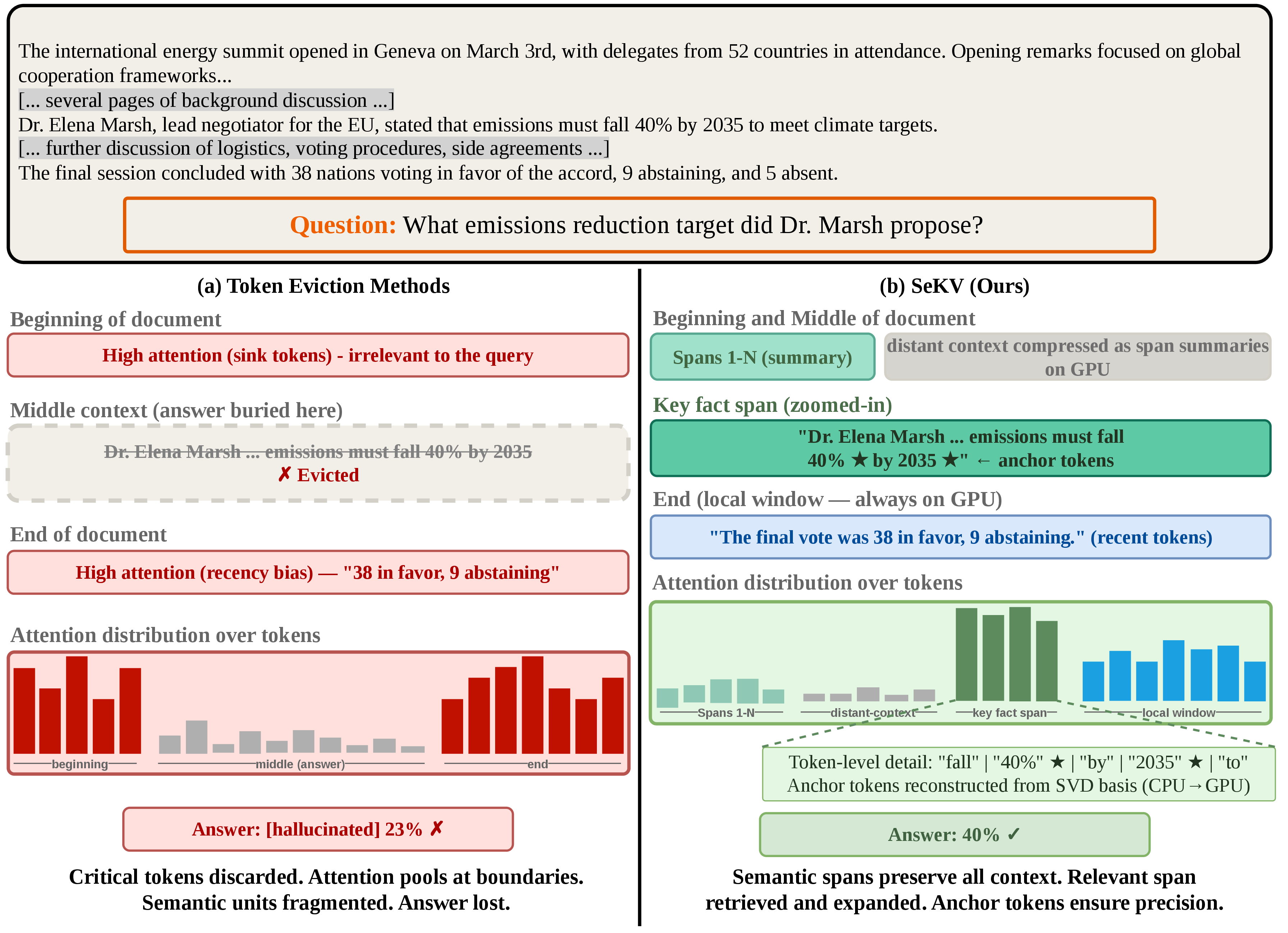
Large language models (LLMs) are increasingly expected to reason over long contexts in applications such as document analysis [1], multi-turn dialogue [2], and agentic planning [3]. While recent models advertise context windows of 128K tokens or more, using these contexts in practice remains expensive: the Key-Value (KV) cache grows linearly with sequence length and must be retained throughout decoding. As a result, full KV caching can become prohibitively memory-intensive, making long-context inference difficult to deploy without compression or memory-efficient cache management. This creates a practical challenge distinct from simply extending the context window: long-context models must not only accept long inputs, but also preserve access to relevant evidence under tight memory constraints.
Recent KV cache management methods reduce inference cost through token eviction, quantization, merging, retrieval, or offloading [4]–[8]. However, most methods either treat context as a flat sequence of token-level states or apply semantic grouping with a static compression policy fixed at prefill time [9]–[11]. Both choices are limiting for long-context reasoning. Token-level compression can fragment coherent evidence or permanently discard information, while static semantic compression cannot recover token-level detail when a compressed span becomes relevant later in decoding. This is especially problematic when evidence that appears peripheral early becomes a critical logical anchor for a later query. Therefore, in this paper, we argue that long-context KV caching requires not only stronger compression, but a different memory organization: one that stores context at variable resolution and dynamically zooms into the appropriate level of detail based on query relevance.
We introduce SeKV (Semantic KV Cache), a resolution-adaptive semantic KV cache for efficient long-context LLM inference. SeKV organizes the KV cache as a hierarchical semantic memory. First, the input context is segmented into semantically coherent spans using token surprisal as a boundary signal, which is available from the model’s prefill forward pass and often peaks at semantic transitions such as topic shifts and entity introductions [12]. High-surprisal anchor tokens at span boundaries are preserved at full resolution on GPU, as they carry concentrated semantic information useful for later routing and reconstruction. Second, each span is represented by a lightweight summary vector on GPU (used for efficient coarse routing) and a low-rank SVD basis on CPU that compactly encodes the span’s token-level structure for faithful reconstruction. Third, a trained zoom-in mechanism dynamically selects which spans to expand to token-level resolution during decoding, triggering asynchronous CPU-to-GPU fetches of SVD bases for relevant spans while GPU computation proceeds in parallel. Crucially, SeKV avoids irreversible token eviction: each span is represented by GPU-resident summary vectors for coarse routing and CPU-resident low-rank bases that enable approximate token-level reconstruction on demand. Across four long-context understanding benchmarks, SeKV achieves 5.9% improvement over the strongest semantic compression baseline while reducing GPU memory consumption by 53.3% compared to full KV caching at 128K context length.
In summary, this work makes three contributions. (1) we propose SeKV, a resolution-adaptive semantic KV cache that stores context at multiple resolutions and dynamically adjusts cache detail based on query relevance during decoding. (2) We introduce entropy-guided span segmentation, which uses token surprisal during prefilling to identify coherent semantic spans and preserve high-surprisal anchor tokens at full resolution for reliable later retrieval. (3) We design a dual-representation KV structure with GPU-resident span summaries for coarse routing, CPU-resident low-rank bases for approximate token-level reconstruction, and a trained zoom-in mechanism that selectively expands only the query-relevant spans during decoding.
2 Related Work↩︎
KV cache compression and eviction. The dominant approach to KV cache compression is token eviction, where tokens are permanently discarded based on attention statistics [4], [5], [13]–[15]. Head-aware methods distinguish retrieval heads from streaming heads to apply sparsity selectively [16], [17], while cross-layer methods exploit the high similarity between adjacent layer KV states to merge or share representations [6], [18]–[20]. To scale beyond GPU memory limits, retrieval-based systems offload KV pairs to CPU and fetch relevant entries on demand using lightweight GPU-resident proxies [7], [8], [21]. DesireKV [22] targets reasoning models specifically by jointly considering attention-derived importance and quantization sensitivity to make differentiated per-token compression decisions. While collectively effective, these methods all fix compression decisions at prefill time, operate at the token level, and permanently discard information — properties that limit their ability to recover evidence that becomes relevant only during generation. SeKV differs fundamentally: it organizes context into semantic spans, avoids irreversible token eviction through a GPU–CPU memory hierarchy, and dynamically recovers token-level detail on demand with a trained zoom-in mechanism.
Semantic KV cache compression. Recent methods introduce semantically structured KV compression by grouping tokens before compression. ChunkKV [9] preserves local coherence by selecting contiguous token chunks; SemantiCache [10] segments context, clusters tokens by key similarity, and merges each cluster into representative KV pairs; and SentenceKV [11] stores sentence-level semantic vectors on GPU and offloads selected token-level KV pairs to CPU for dynamic retrieval during decoding. These methods show that semantic structure can improve cache efficiency over flat token eviction. However, their semantic units and retained cache representations are largely fixed during prefill, making it difficult to recover finer-grained evidence outside the retained token pool when it becomes relevant later. SeKV addresses this limitation with entropy-guided spans, GPU-resident routing summaries, CPU-resident low-rank bases, and a trained zoom-in mechanism that reconstructs query-relevant spans on demand.
3 SeKV↩︎
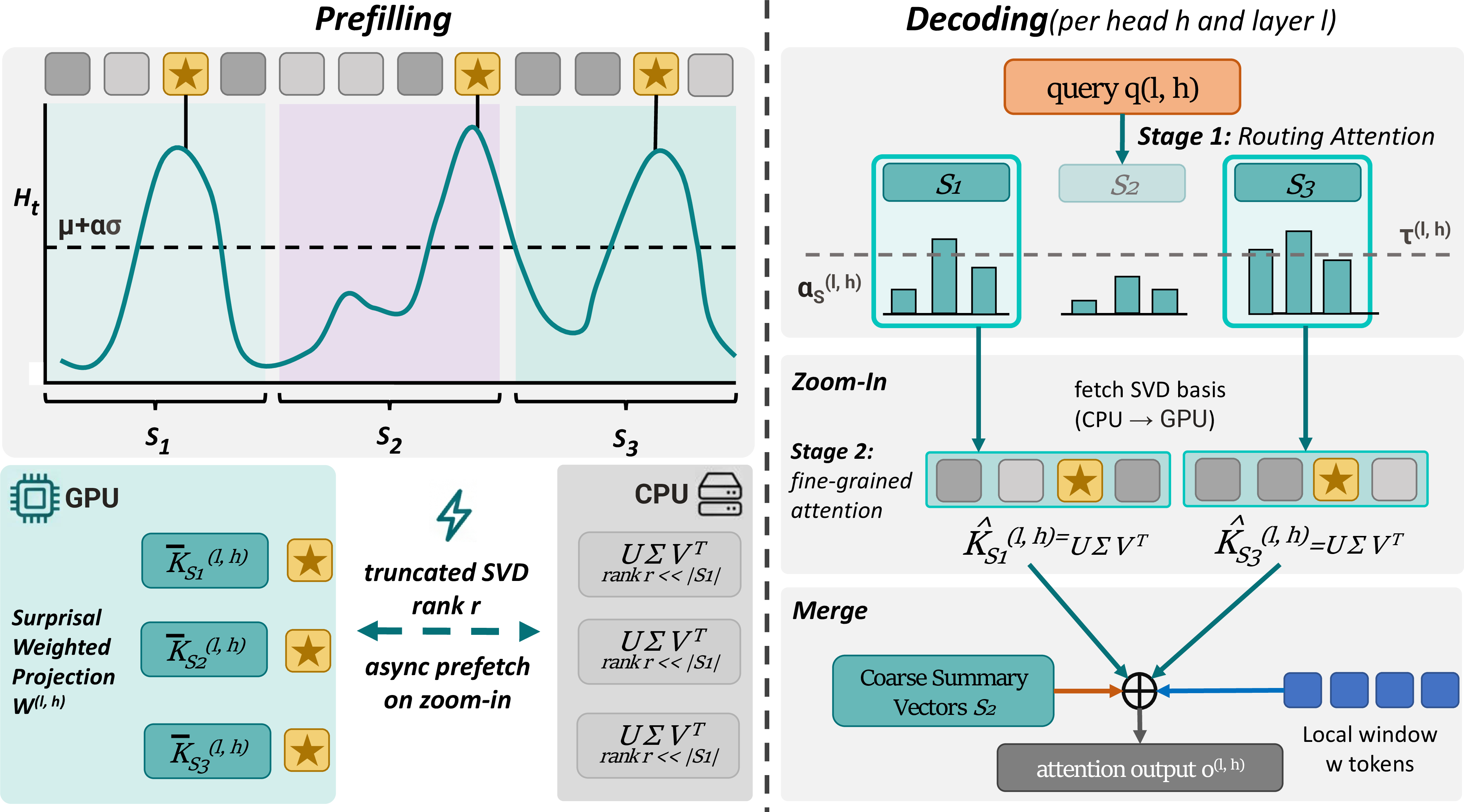
SeKV reorganizes the KV cache from a flat token-level sequence into a hierarchical semantic memory. As illustrated in Figure 2, the context is segmented into semantically coherent spans, each represented at two resolutions simultaneously: a compact summary vector on GPU for efficient coarse routing, and a low-rank SVD basis on CPU for faithful token-level reconstruction on demand. A trained zoom-in mechanism with per-head per-layer routing projections, a learned per-span rank budget, and learned thresholds dynamically selects which spans to expand during decoding and at what fidelity. We describe each component below.
3.1 Entropy-Guided Span Segmentation↩︎
SeKV segments the input context into semantically coherent spans using token-level surprisal as a zero-cost boundary signal. During prefilling, the surprisal of the token at each position \(t\) is computed as \[H_t = -\log p\big(x_t \mid x_{<t}\big),\] where \(x_t\) is the token at position \(t\) and \(x_{<t} = (x_1, \ldots, x_{t-1})\) denotes the preceding tokens. This quantity is already produced by the prefill forward pass and requires no additional computation. High-surprisal tokens often mark semantic transitions such as topic shifts, entity introductions, and logical turns [12]. We therefore treat positions where \(H_t > \mu + \alpha\sigma\) as span boundaries, where \(\mu\) and \(\sigma\) are the mean and standard deviation of surprisal over the sequence and \(\alpha\) controls boundary sensitivity. These boundary tokens are retained as anchor tokens at full resolution on GPU, while the tokens between two neighboring anchors form a semantic span \(S\).
Compared with fixed-size chunking [9] or delimiter-based splitting [10], surprisal-based segmentation is content-adaptive and requires no external tagger, splitter, or additional model. It allocates finer resolution to information-dense regions, which produce shorter spans and more anchors, while compressing lower-density text into longer spans. The resulting spans are then encoded into the dual-resolution representation described in Section 3.2.
3.2 Dual-Resolution Span Representation and Memory Hierarchy↩︎
Each semantic span \(S\) is represented at two resolutions: a GPU-resident summary used for efficient span-level routing, and a CPU-resident low-rank basis used for approximating token-level reconstruction when the span is selected for zoom-in.
3.2.0.1 Summary vector (GPU).
For each token \(t \in S\), let \(H_t\) denote its surprisal under the frozen LLM during prefilling. We first convert token surprisals into normalized span-local weights: \[w_t = \frac{H_t}{\sum_{k \in S} H_k}. \label{eq:surprisal95weight}\tag{1}\] This weights non-anchor tokens by their residual surprisal.
For each layer \(l\) and attention head \(h\), let \(K_t^{(l,h)} \in \mathbb{R}^{d_h}\) denote the key vector of token \(t\), where \(d_h\) is the head dimension (\(d_h = 128\) on Llama-3-8B). We compute a compact summary key \(\bar{K}_S^{(l,h)} \in \mathbb{R}^{d'}\), where \(d' \ll d_h\) is the routing dimension (\(d' = 32\)), by projecting token keys with a learned per-head, per-layer projection \(W^{(l,h)} \in \mathbb{R}^{d' \times d_h}\) and taking a normalized surprisal-weighted average: \[\bar{K}_S^{(l,h)} = \frac{ \sum_{t \in S} w_t W^{(l,h)} K_t^{(l,h)} }{ \left\| \sum_{t \in S} w_t W^{(l,h)} K_t^{(l,h)} \right\|_2 }, \label{eq:summary95key}\tag{2}\] where the per-head, per-layer projection \(W^{(l,h)}\) lets each head-layer pair learn its own relevance space, since attention patterns vary across heads and layers [23]. This summary is used only for routing. We additionally keep on GPU the surprisal-weighted mean key and value in the original space, \(\bar{k}_S^{(l,h)} = \sum_{t \in S} w_t K_t^{(l,h)}\) and \(\bar{v}_S^{(l,h)} = \sum_{t \in S} w_t V_t^{(l,h)}\), both in \(\mathbb{R}^{d_h}\), which serve as the coarse contribution of a non-expanded span in the output attention (Sec. 3.3).
At each decoding step, we project the current query into the same routing space as the span summaries: \[q^{(l,h)} = W^{(l,h)} q_t^{(l,h)} \in \mathbb{R}^{d'}. \label{eq:query95projection}\tag{3}\] Since zoom-in is an independent per-span decision, we use a sigmoid relevance gate rather than a competitive softmax: \[\tilde{\alpha}_S^{(l,h)} = \mathrm{sig}\!\left( \frac{ q^{(l,h)} \left(\bar{K}_S^{(l,h)}\right)^\top }{ \sqrt{d'} } + \log |S| \right), \label{eq:routing95gate}\tag{4}\] where \(\mathrm{sig}(x) = 1/(1 + e^{-x})\) is the logistic function. The \(\log |S|\) term acts as a monotone size prior, preventing longer spans from being systematically under-selected. Because \(\tilde{\alpha}_S^{(l,h)}\) is span-independent, the threshold in Sec. 3.3 remains stable across context lengths.
3.2.0.2 Low-rank SVD basis with a learned rank budget (CPU).
To support token-level reconstruction without keeping full KV pairs on GPU, we store a compact low-rank representation of each span on CPU. For each layer \(l\) and head \(h\), let \(K_S^{(l,h)} \in \mathbb{R}^{|S| \times d_h}\) denote the key matrix formed by stacking the token keys in span \(S\). We compute its truncated SVD up to a maximum rank \(R = \min(|S|, d_h, R_{\max})\), for a fixed cap \(R_{\max}\), \[K_S^{(l,h)} = \sum_{i=1}^{R} \sigma_{S,i}^{(l,h)}\, u_{S,i}^{(l,h)} {\left(v_{S,i}^{(l,h)}\right)}^\top, \label{eq:key95svd}\tag{5}\] with left and right singular vectors \(u_{S,i}^{(l,h)} \in \mathbb{R}^{|S|}\) and \(v_{S,i}^{(l,h)} \in \mathbb{R}^{d_h}\). Rather than truncating at a single global rank, a lightweight predictor \(g_\phi\) assigns per-component soft gates \[m_{S,i}^{(l,h)} = \mathrm{sig}\!\left(g_\phi\big(\sigma_{S,\cdot}^{(l,h)}, \bar{K}_S^{(l,h)}\big)_i\right) \in (0,1), \label{eq:rank95gates}\tag{6}\] computed from the singular spectrum and the span summary, and the gated reconstruction is \[\hat{K}_S^{(l,h)} = \sum_{i=1}^{R} m_{S,i}^{(l,h)}\, \sigma_{S,i}^{(l,h)}\, u_{S,i}^{(l,h)} {\left(v_{S,i}^{(l,h)}\right)}^\top. \label{eq:key95reconstruction}\tag{7}\] The effective rank of span \(S\) is \(r_S^{(l,h)} = \sum_i m_{S,i}^{(l,h)}\). At deployment, components with negligible gates are dropped, so the stored and transferred factors \(U_S^{(l,h)} \in \mathbb{R}^{|S| \times r_S}\), \(\Sigma_S^{(l,h)} \in \mathbb{R}^{r_S \times r_S}\), and \(V_S^{(l,h)} \in \mathbb{R}^{d_h \times r_S}\) adapt per span: information-dense spans retain more components, redundant spans fewer. We apply the same gated decomposition to the value matrix \(\mathcal{V}_S^{(l,h)} \in \mathbb{R}^{|S| \times d_h}\), obtaining its own gates \(m_{S,j}^{\mathcal{V},(l,h)}\) and factors \(U_S^{\mathcal{V},(l,h)}, \Sigma_S^{\mathcal{V},(l,h)}, V_S^{\mathcal{V},(l,h)}\), which are likewise stored on CPU. Here \(V_S^{(l,h)}\) and \(V_S^{\mathcal{V},(l,h)}\) denote the right singular vectors of the key and value matrices, while \(\mathcal{V}_S^{(l,h)}\) denotes the value matrix itself.
Because entropy-guided segmentation groups tokens into coherent spans, their KV matrices are often more compressible than arbitrary token blocks, so a small number of components can preserve most span information. Storing a retained rank-\(r_S\) factorization costs \(r_S(|S| + d_h + 1)\) values per head and layer, compared with \(|S|d_h\) for the full key matrix, yielding savings when \(r_S \ll d_h\). The representation is therefore compact in transfer volume, although the left factor still scales with span length. To avoid unnecessary overhead, spans shorter than \(L_{\min}\) are kept at full resolution on GPU. Key and value decompositions are computed once during prefilling; randomized truncated SVD keeps this step parallelizable and amortizes its cost over decoding.
Together, these representations define the memory hierarchy in SeKV. Anchor tokens remain uncompressed on GPU and always participate in fine-grained attention, while span summaries support coarse routing. Low-rank SVD bases for non-anchor tokens reside on CPU and are fetched asynchronously only for selected spans. During decoding, SeKV overlaps GPU computation with CPU–GPU prefetching, following pipelined orchestration designs [7]. Unlike retrieval-based offloading methods that transfer full token-level KV pairs from CPU [11], [21], SeKV transfers compact low-rank bases and reconstructs only zoomed spans, reducing transfer volume while avoiding irreversible token eviction.
3.3 Trained Zoom-In Mechanism↩︎
At each decoding step, SeKV first routes over span summary vectors. For each layer \(l\) and head \(h\), the routing gate assigns a per-span relevance probability \(\tilde{\alpha}_S^{(l,h)}\), and a learned per-head per-layer threshold \(\tau^{(l,h)}\) determines whether span \(S\) is expanded: \[z_S^{(l,h)} = \mathbf{1}\!\left[\tilde{\alpha}_S^{(l,h)} > \tau^{(l,h)}\right]. \label{eq:zoom95decision}\tag{8}\] Per-head thresholds matter because heads have different selectivity: retrieval heads may expand many distant spans, while streaming heads should rarely trigger expansion. Each decoding step then performs a single attention computation over a mixed-resolution memory. Anchor tokens always contribute full key–value pairs. Non-expanded spans contribute one coarse entry, given by their retained mean key and value \(\bar{k}_S^{(l,h)}\) and \(\bar{v}_S^{(l,h)}\), with a \(\log |S|\) correction added to the pre-softmax score so that one summary competes proportionally to the \(|S|\) tokens it represents [24]. Expanded spans fetch their low-rank bases from CPU, reconstruct token-level KV pairs via Eq. 7 , and enter attention at full resolution. Since coarse summaries and reconstructed tokens share the same softmax, zooming refines a span’s contribution rather than adding a separate attention path, and no span is dropped from context.
For fair comparison with fixed-budget baselines, we define the budget as the peak GPU-resident KV during a decoding step, including persistent anchors, summaries, coarse means, and any spans reconstructed at that step. The learned thresholds \(\tau^{(l,h)}\) provide the default expansion rule. If the selected spans exceed the budget, we keep spans in decreasing order of \(\tilde{\alpha}_S^{(l,h)}\) until the budget is filled. Thus, the threshold sets the operating point, while the cap enforces the matched memory budget.
We train only the lightweight routing components while keeping the base LLM frozen, using a straight-through estimator [25] for the binary decision in Eq. 8 . The objective combines four terms: \[\mathcal{L} = \mathcal{L}_{\text{distill}} + \lambda_1 \mathcal{L}_{\text{zoom}} + \lambda_2 \mathcal{L}_{\text{recon}} + \lambda_3 \mathcal{L}_{\text{budget}}. \label{eq:total95loss}\tag{9}\]
3.3.0.1 Distillation.
The distillation loss aligns SeKV with a full-KV teacher and provides the end-task signal that flows, through the straight-through gate, to both the routing projections and the thresholds: \[\mathcal{L}_{\text{distill}} = D_{\text{KL}}\!\left(p_{\text{full}} \,\|\, p_{\text{\mathrm{\small SeKV}}}\right).\]
3.3.0.2 Zoom supervision.
We supervise the routing probability directly against a teacher-derived target rather than against the thresholded decision, which keeps the loss well-posed and free of the trainable threshold. Let \(a_S^{(l,h)} = \sum_{t \in S} \alpha_t^{(l,h),\mathrm{teacher}}\) be the teacher attention mass on span \(S\), and let \(\mathcal{C}_\rho^{(l,h)}\) be the smallest set of spans whose cumulative mass reaches a fixed fraction \(\rho\). The fixed binary target is \[y_S^{(l,h)} = \mathbf{1}\!\left[S \in \mathcal{C}_\rho^{(l,h)}\right],\] which depends only on the teacher and not on \(\tau^{(l,h)}\). The zoom loss is a positive-weighted binary cross-entropy on the routing probability, \[\mathcal{L}_{\text{zoom}} = \sum_l \sum_h \sum_S \mathrm{BCE}_{w^+}\!\left(\tilde{\alpha}_S^{(l,h)},\, y_S^{(l,h)}\right),\] where positive weight \(w^+\) compensates for the rarity of relevant spans. Since the target is fixed and independent of \(\tau^{(l,h)}\), this loss trains the routing projections to separate relevant from irrelevant spans without letting the threshold define its own supervision.
3.3.0.3 Reconstruction.
The reconstruction loss supervises the per-span rank budget through the per-component soft gates \(m_{S,i}^{(l,h)} \in (0,1)\) predicted by \(g_\phi\) (Eq. 6 ), and their value counterparts \(m_{S,j}^{\mathcal{V},(l,h)}\). Since the singular components are orthonormal, the gated approximation error of a single factorization is \(\mathcal{E}(m, \sigma) = \sum_i (1 - m_i)^2 \sigma_i^2\). Summing over keys and values, heads, layers, and spans gives \[\begin{align} \mathcal{L}_{\text{recon}} ={} & \sum_{l,h,S} \mathcal{E}\big(m_S^{(l,h)},\, \sigma_S^{(l,h)}\big) \\ & + \sum_{l,h,S} \mathcal{E}\big(m_S^{\mathcal{V},(l,h)},\, \sigma_S^{\mathcal{V},(l,h)}\big) \end{align}\] where \(\sigma_S^{(l,h)}\) and \(\sigma_S^{\mathcal{V},(l,h)}\) are the singular values of the key and value matrices of span \(S\). This is differentiable in the gates and therefore trains the rank predictor \(g_\phi\). The singular values and vectors come from the frozen keys and values and are treated as constants (no gradient flows through the SVD), which avoids the instability of SVD backpropagation under near-degenerate singular values.
3.3.0.4 Budget.
The reconstruction loss alone is minimized by retaining every component, and distillation likewise prefers more rank and more expansions, so a cost term is required to make the rank budget and the threshold meaningful: \[\mathcal{L}_{\text{budget}} = \sum_l \sum_h \sum_S \left( z_S^{(l,h)} + \beta \sum_i m_{S,i}^{(l,h)} \right).\] The first term penalizes the number of expanded spans and, through the straight-through gate, encourages higher thresholds when expansions are too costly. The second term penalizes the total retained rank \(\sum_i m_{S,i}^{(l,h)}\), balancing \(\mathcal{L}_{\text{recon}}\) so that rank is allocated only where it meaningfully reduces error. The coefficient \(\beta > 0\) sets the relative cost of retained rank against span expansion, controlling how the budget is split between transferring more spans and reconstructing each at higher rank.
3.3.0.5 Learnable parameters.
SeKV keeps the base LLM frozen and learns only the routing projections \(\{W^{(l,h)}\}\), the zoom thresholds \(\{\tau^{(l,h)}\} \in \mathbb{R}^{L \times H}\), and the shared rank-gate predictor \(g_\phi\). Llama-3-8B [26] uses grouped-query attention with \(L=32\) layers, \(H=32\) query heads, and \(8\) key-value heads. Each query head routes against a summary built from its group’s shared key-value head, so the projections are indexed per query head, with \(\{W^{(l,h)}\} \in \mathbb{R}^{L \times H \times d' \times d_h}\). With \(d_h=128\) and \(d'=32\), the projections account for about \(4.19\)M parameters, the thresholds for \(L \times H = 1024\), and \(g_\phi\) for under \(0.1\)M, totaling approximately \(4.3\)M, about \(0.05\%\) of the base model.
4 Experiments and Results↩︎
4.1 Experimental Setup↩︎
Benchmarks. We evaluate SeKV on four long-context benchmarks: LongBench [27], RULER [28], InfiniteBench [29], and Needle-in-a-Haystack (NIAH) [30]. Together, these benchmarks cover realistic long-document understanding, controlled synthetic retrieval and reasoning, ultra-long context stress tests, and targeted retrieval fidelity up to 128K tokens. We additionally evaluate GSM8K [31] in a many-shot setting to test whether compression preserves step-by-step reasoning over long prompts. Refer to Appendix 7 for more details.
| LongBench | RULER | ||||||||||
|---|---|---|---|---|---|---|---|---|---|---|---|
| 2-6 (lr)7-11 Method | |||||||||||
| Full KV | 43.21 | 50.34 | 51.18 | 41.83 | 55.47 | 73.67 | 81.94 | 88.35 | 68.38 | 90.74 | |
| StreamingLLM [15] | 28.43 | 38.41 | 39.17 | 34.82 | 42.31 | 41.32 | 52.17 | 58.43 | 38.24 | 61.87 | |
| H2O [13] | 31.72 | 43.84 | 44.52 | 37.63 | 47.18 | 48.71 | 61.33 | 67.82 | 45.17 | 71.24 | |
| SnapKV [4] | 34.18 | 46.23 | 47.11 | 38.91 | 49.34 | 54.83 | 68.42 | 74.31 | 51.63 | 77.48 | |
| PyramidKV [5] | 35.44 | 47.13 | 48.02 | 39.74 | 50.17 | 56.17 | 70.14 | 76.23 | 53.41 | 79.33 | |
| ChunkKV [9] | 36.82 | 48.31 | 49.14 | 40.83 | 51.42 | 58.34 | 72.83 | 78.41 | 55.72 | 81.17 | |
| SemantiCache [10] | 37.14 | 48.73 | 49.61 | 41.17 | 51.88 | 59.12 | 73.47 | 79.18 | 56.33 | 82.04 | |
| SentenceKV [11] | 37.83 | 49.12 | 49.93 | 41.44 | 52.31 | 60.43 | 74.82 | 80.37 | 57.84 | 83.41 | |
| (Ours) | 39.47 | 50.18 | 51.02 | 42.63 | 54.71 | 63.84 | 78.43 | 84.17 | 61.23 | 87.34 | |
| InfiniteBench | NIAH | ||||||||||
| 2-6 (lr)7-11 Method | |||||||||||
| Full KV | 21.16 | 25.27 | 28.88 | 22.77 | 36.51 | 76.72 | 85.23 | 91.52 | 72.39 | 95.28 | |
| StreamingLLM [15] | 11.43 | 14.82 | 17.31 | 12.64 | 22.17 | 38.43 | 47.82 | 54.17 | 34.71 | 58.34 | |
| H2O [13] | 13.72 | 17.43 | 20.14 | 14.83 | 25.38 | 47.83 | 58.41 | 64.83 | 43.72 | 68.47 | |
| SnapKV [4] | 15.84 | 19.73 | 22.47 | 16.72 | 28.14 | 54.17 | 66.83 | 73.42 | 51.34 | 76.83 | |
| PyramidKV [5] | 16.43 | 20.81 | 23.62 | 17.44 | 29.37 | 56.43 | 68.72 | 75.83 | 53.17 | 78.41 | |
| ChunkKV [9] | 17.12 | 21.83 | 24.71 | 18.23 | 30.84 | 59.84 | 72.14 | 79.23 | 56.83 | 81.72 | |
| SemantiCache [10] | 17.83 | 22.47 | 25.33 | 18.84 | 31.42 | 61.17 | 73.83 | 80.74 | 58.14 | 83.17 | |
| SentenceKV [11] | 18.34 | 23.14 | 26.07 | 19.47 | 32.17 | 63.42 | 75.47 | 82.13 | 60.23 | 84.83 | |
| (Ours) | 19.72 | 24.83 | 27.94 | 21.13 | 34.83 | 68.83 | 81.34 | 87.42 | 65.74 | 91.17 | |
Baselines. We compare SeKV with full KV caching and representative KV-cache compression baselines. Token-level methods include StreamingLLM [15], H2O [13], SnapKV [4], and PyramidKV [5]; semantic or chunk-level methods include ChunkKV [9], SemantiCache [10], and SentenceKV [11]. All compression methods are evaluated under matched GPU-resident KV memory budgets, with main results at 10% of full KV and additional 5%, 15%, and 20% budget results in the ablation study. Further baseline details are provided in Appendix 7.
Backbone models. We evaluate SeKV on five backbones: Llama-3.2-3B-Instruct, Llama-3-8B, Llama-3.1-8B-Instruct [26], Mistral-7B-Instruct-v0.3 [32], and Qwen2.5-14B-Instruct [33]. This suite covers different model scales and families, allowing us to test whether SeKV generalizes across backbones. Within each benchmark, all methods use the same backbone, tokenizer, decoding strategy, and maximum generation length. For contexts beyond a model’s default limit, we enable its available long-context configuration; for settings above 128K tokens, we use Qwen2.5-14B-Instruct-1M when full-context evaluation is required.
Tasks & Metrics. We follow each benchmark’s official protocol, reporting average F1 on LongBench QA subsets, average accuracy on RULER, accuracy on the InfiniteBench Retrieve subset, retrieval accuracy on NIAH, and exact-match accuracy on GSM8K.
Implementation and inference details. SeKV is implemented in PyTorch3 with HuggingFace Transformers4. The base LLM remains frozen; we train only the per-head per-layer routing projections, the zoom-in thresholds, and the shared rank-gate predictor \(g_\phi\) (Section 3.3). These lightweight components are trained on long documents from RedPajama [34] (arXiv, books, and code subsets), with the zoom objective supervised only at mined query positions whose teacher attention concentrates beyond a local window of \(w=512\) tokens; no instruction or synthetic-retrieval data is used, and the training corpus is disjoint from LongBench, RULER, InfiniteBench, NIAH, and GSM8K. Training uses AdamW [35] (learning rate \(1\times10^{-3}\), weight decay \(0.01\), cosine decay with \(10\%\) warmup) in bf16 for roughly \(3\)K steps over about \(0.5\)B tokens, with an \(8\)K \(\rightarrow\) \(32\)K length curriculum and an effective batch of \(8\) sequences (one per GPU). We use a maximum SVD rank \(R=32\) with the per-span effective rank set by \(g_\phi\), summary dimension \(d'=32\), boundary sensitivity \(\alpha=1.0\), permissive threshold initialization \(\tau=0.05\), and loss weights \(\lambda_1=1.0\) (zoom), \(\lambda_2=0.5\) (reconstruction), and \(\lambda_3=0.1\) (budget, annealed from \(0\) over the first half of training), with rank sub-weight \(\beta=0.1\), positive class weight \(w^+=10\), and coverage fraction \(\rho=0.9\). Training a single backbone takes \(2\) to \(6\) hours on one \(8\times\)NVIDIA A100 (80GB) node, with Qwen2.5-14B-Instruct at the upper end; the full hyperparameter list is given in Appendix 6. At inference time, we use greedy decoding with temperature \(0\) and benchmark-specific maximum generation lengths. Anchor tokens, span summaries, and coarse span means remain on GPU, while low-rank SVD bases are stored on CPU and fetched asynchronously when zoom-in is triggered; to match a target budget, spans are expanded in decreasing routing-score order until the GPU-resident KV budget is reached. LongBench, RULER, NIAH, and GSM8K are evaluated on a single A100 80GB GPU whenever the method fits. For InfiniteBench and full-KV reference runs that exceed single-device memory, we use tensor parallelism across up to \(8\) A100 80GB GPUs. All efficiency comparisons among compression methods use the single-GPU deployment setting.
4.2 Long-Context Reasoning↩︎
Long-context benchmark performance. Table 1 shows that SeKV is the strongest compressed-cache method across all four benchmarks and all five backbone models. SeKV wins every compressed setting: 20 out of 20 benchmark–model comparisons. Averaged over all settings, SeKV improves over the strongest baseline, SentenceKV, by 5.9% under the same 10% KV budget. The gains are especially large on retrieval-heavy benchmarks: +5.68 on NIAH and +3.63 on RULER, showing that adaptive zoom-in is particularly useful when a small piece of evidence must be recovered from a long context. On more heterogeneous benchmarks, the gains remain consistent: +1.48 on LongBench and +1.85 on InfiniteBench. These results support the central claim of SeKV: static compression preserves coarse context, but dynamic resolution recovery is needed to retrieve fine-grained evidence at generation time. We further isolate the contribution of each SEKV component and analyze sensitivity to the GPU-resident KV budget and key hyperparameters in Appendix 8.
Comparison to Full KV and model scaling. Despite using only 10% of the KV budget, SeKV remains close to Full KV, with average gaps of only 0.80 points on LongBench and 1.23 points on InfiniteBench. The gap is larger on retrieval-sensitive benchmarks such as RULER and NIAH, but SeKV still substantially narrows it compared to prior methods. Its gains over SentenceKV are also stable across backbones, ranging from +2.94 to +3.83, with the largest improvement on Qwen2.5-14B, suggesting that stronger models benefit more from resolution-adaptive cache access.
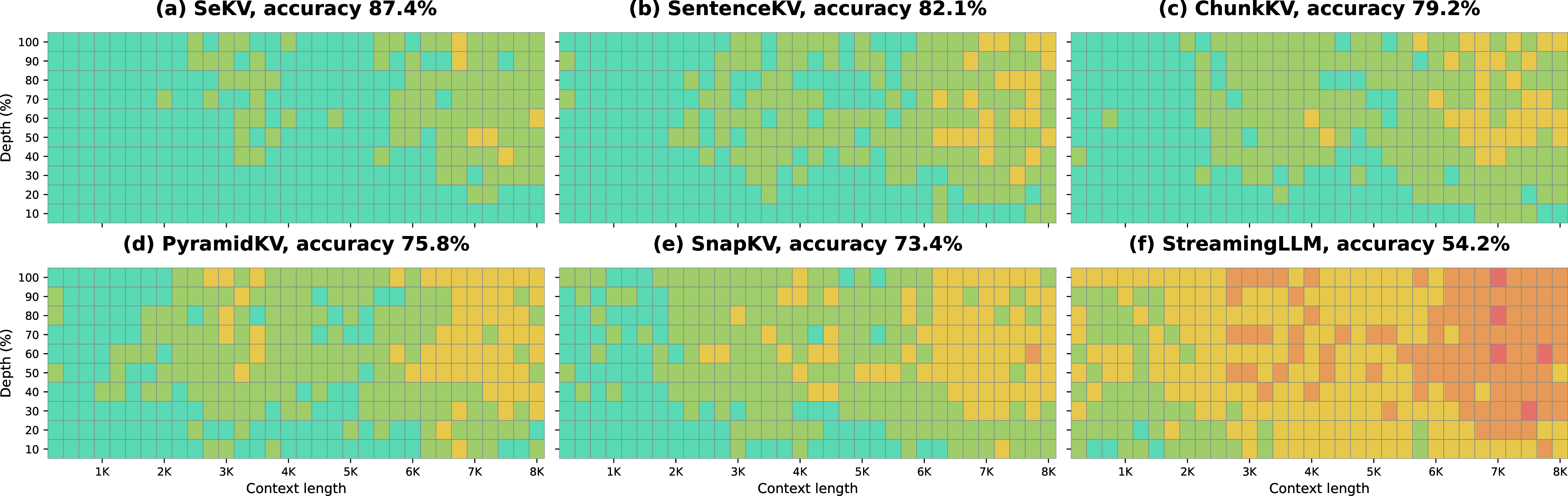
Needle retrieval behavior. Figure 3 shows NIAH heatmaps for Llama-3.1-8B with a fixed KV cache size of 128. SeKV maintains strong retrieval across context lengths and needle depths, with most cells remaining high-success. Prior methods degrade more noticeably at longer contexts and deeper insertions: SentenceKV and ChunkKV remain competitive but show more failures, while token-eviction methods such as SnapKV, PyramidKV, and StreamingLLM exhibit broader low-success regions. This indicates that SeKV’s gains are consistent across the length–depth space rather than concentrated on easy needle positions.
| SnapKV | PyramidKV | ChunkKV | SentenceKV | |
|---|---|---|---|---|
| 53.4 | 54.2 | 55.6 | 56.1 | 58.4 |
| 61.7 | 63.2 | 64.6 | 65.4 | 67.8 |
| 68.2 | 70.3 | 74.9 | 76.8 | 79.3 |
| 66.7 | 68.1 | 69.3 | 70.4 | 72.5 |
| 77.9 | 79.4 | 80.7 | 82.1 | 84.5 |
| Method | Input | Output | Lat. (s) \(\downarrow\) | Throughput (T/S) \(\uparrow\) |
|---|---|---|---|---|
| FullKV | 4096 | 1024 | 43.60 | 105.92 |
| StreamingLLM | 4096 | 1024 | 34.10 | 132.40 |
| ChunkKV | 4096 | 1024 | 37.52 | 118.85 |
| SentenceKV | 4096 | 1024 | 39.84 | 112.64 |
| 4096 | 1024 | 38.05 | 120.11 | |
| FullKV | 4096 | 4096 | 175.50 | 37.73 |
| StreamingLLM | 4096 | 4096 | 148.92 | 44.23 |
| ChunkKV | 4096 | 4096 | 164.55 | 40.58 |
| SentenceKV | 4096 | 4096 | 169.64 | 38.91 |
| 4096 | 4096 | 166.72 | 40.31 | |
| FullKV | 8192 | 1024 | 46.48 | 184.08 |
| StreamingLLM | 8192 | 1024 | 33.94 | 245.35 |
| ChunkKV | 8192 | 1024 | 37.83 | 228.96 |
| SentenceKV | 8192 | 1024 | 40.52 | 210.74 |
| 8192 | 1024 | 38.64 | 223.18 | |
| FullKV | 8192 | 4096 | 183.42 | 55.93 |
| StreamingLLM | 8192 | 4096 | 150.86 | 70.41 |
| ChunkKV | 8192 | 4096 | 164.78 | 65.14 |
| SentenceKV | 8192 | 4096 | 171.26 | 60.82 |
| 8192 | 4096 | 166.95 | 64.21 |
4.3 Many-Shot Reasoning↩︎
Table 2 evaluates whether KV-cache compression preserves reasoning behavior in a long-prompt setting. Unlike NIAH or RULER, GSM8K does not primarily test retrieval of a single hidden fact; instead, the model must preserve many in-context demonstrations that define the reasoning pattern. SeKV achieves the best compressed-cache result across all five backbones, improving over the strongest baseline, SentenceKV, by +2.3 points on average. The gap to FullKV also remains small: SeKV is within 2.4 points of FullKV on average, with particularly strong results on Llama-3.1-8B-Instruct and Qwen2.5-14B-Instruct. These results show that SeKV preserves both sparse retrieval and many-shot reasoning structure.
4.4 Efficiency Analysis↩︎
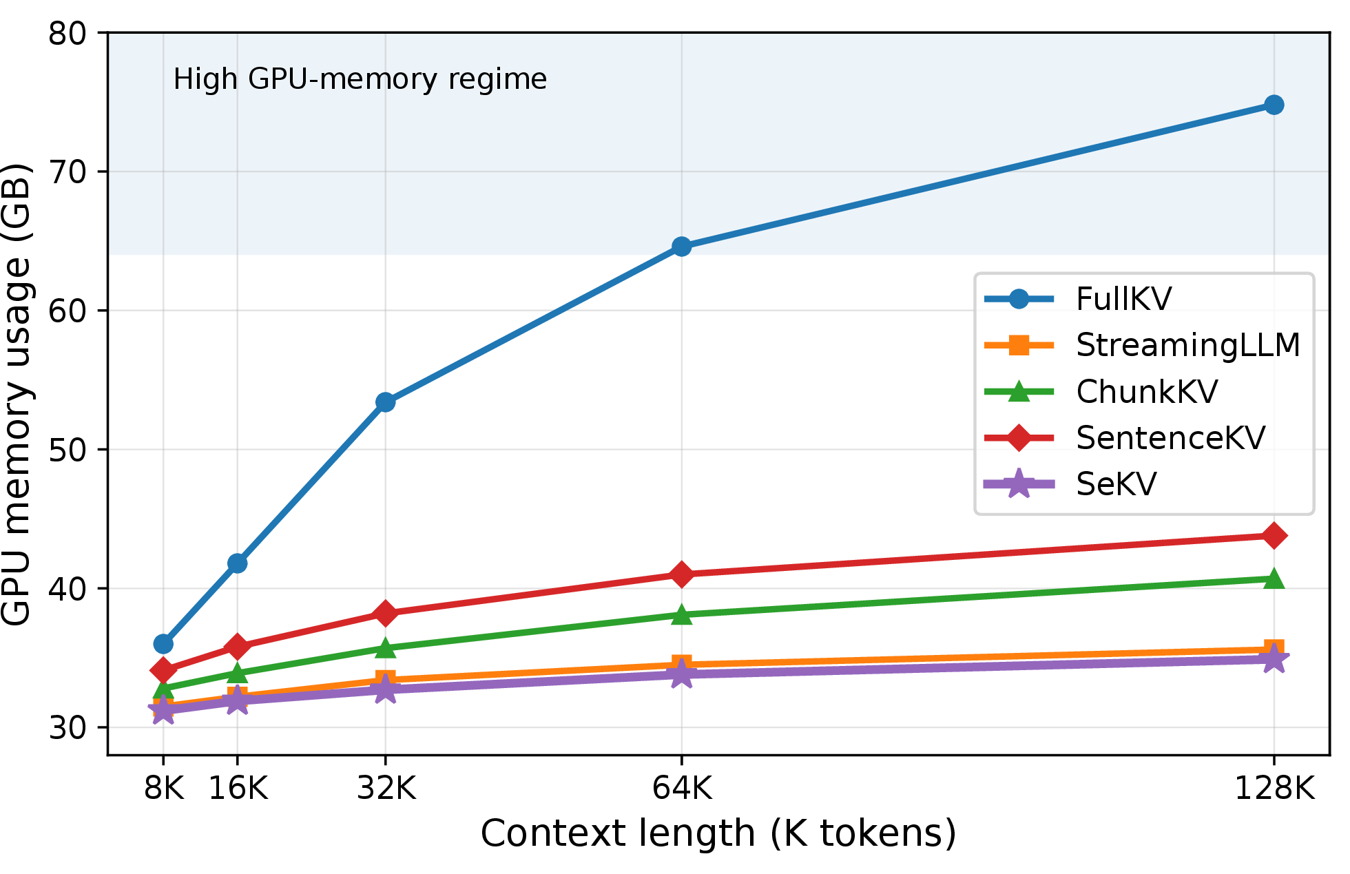
Table 3 compares latency and throughput across input–output lengths. SeKV is consistently faster than FullKV, reducing latency from 43.60s to 38.05s in the 4K/1K setting and from 183.42s to 166.95s in the 8K/4K setting, while improving throughput from 105.92 to 120.11 T/S and from 55.93 to 64.21 T/S. Although StreamingLLM is fastest due to aggressive eviction, it suffers substantial accuracy loss in Table 1. Among semantic methods, SeKV offers the best trade-off: faster than SentenceKV, close to ChunkKV, and substantially more accurate. Figure 4 further shows that SeKV keeps GPU memory nearly flat as context length grows, increasing only from 31.2GB to 34.9GB between 8K and 128K, compared with FullKV’s growth from 36.0GB to 74.8GB. Overall, SeKV improves retrieval fidelity without prohibitive runtime or memory overhead. A detailed memory and computational complexity analysis is provided in Appendix 9.
4.5 Zoom-In Behavior Analysis↩︎
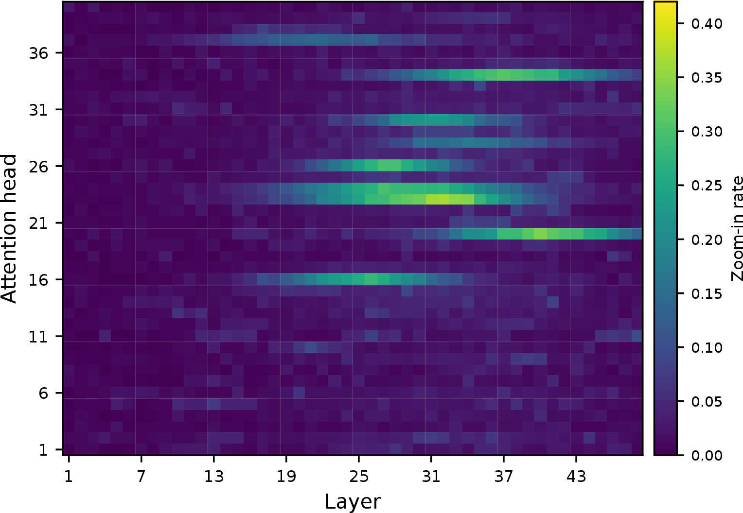
Figure 5 shows that SeKV expands compressed spans selectively rather than uniformly. Zoom-in decisions are sparse and concentrated in specific heads, especially in mid-to-late layers, indicating that only a small subset of retrieval-oriented heads frequently require token-level reconstruction. This supports the use of per-head per-layer thresholds and shows that SeKV saves memory by allocating fine-grained resolution only where needed. Additional heatmaps are provided in Appendix 10.
5 Conclusion↩︎
We introduced SeKV, a resolution-adaptive semantic KV cache for efficient long-context LLM inference. SeKV organizes context into entropy-guided spans, keeps lightweight routing summaries on GPU, and reconstructs low-rank CPU-resident span bases on demand, enabling query-adaptive cache resolution without modifying the base LLM. Across four benchmarks, SeKV outperforms prior KV compression methods, including token-eviction approaches (StreamingLLM [15], H2O [13], SnapKV [4], PyramidKV [5]) and semantic or chunk-level approaches (ChunkKV [9], SemantiCache [10], SentenceKV [11]), improving over the strongest semantic baseline, SentenceKV, by 5.9% on average while reducing GPU memory by 53.3% compared to Full KV at 128K context length. These results show that efficient long-context inference can be achieved by allocating fine-grained resolution only where needed.
Limitations↩︎
SeKV has some limitations worth noting. First, its effectiveness depends on the quality of the semantic span construction. Since SeKV allocates cache resolution based on entropy-guided semantic segmentation, noisy boundaries or poorly calibrated uncertainty estimates can lead to suboptimal memory allocation, especially in documents with highly fragmented discourse, dense tables, code, or unusual formatting. Second, SeKV introduces several design choices, including the entropy threshold for span formation, the number of retained anchor tokens, the rank of span-level low-rank bases, and the retrieval budget for CPU-resident spans. These parameters control the tradeoff between memory usage, reconstruction quality, and decoding latency, and may require validation when transferring to new models or context lengths. Third, although SeKV reduces GPU memory by moving inactive span representations to CPU, this introduces dependence on host-device bandwidth. In settings with slow CPU–GPU transfer or highly adversarial queries that repeatedly activate many distant spans, the latency advantage may be reduced. Finally, SeKV keeps the base LLM frozen and only adds lightweight routing components, which improves deployability but may limit the ability of the model to fully adapt its internal attention behavior to the compressed memory structure. Jointly training the routing module with more expressive span representations or adaptive reconstruction policies is an important direction for future work.
6 Training Details↩︎
6.0.0.1 Training data.
Because SeKV keeps the backbone frozen and trains only the lightweight routing components of Section 3.3, it requires little data and a single language-modeling corpus suffices. We train on long documents from RedPajama [34] (arXiv, books, and code subsets). The distillation and reconstruction objectives use all positions, while the zoom objective is supervised only at mined query positions whose teacher attention is concentrated on non-local spans; the attended spans form the coverage target \(\mathcal{C}_\rho\). This matches the router to the teacher’s own long-range attention without any distribution shift from a QA template, and uses no synthetic retrieval or instruction data, so the training corpus is disjoint from every benchmark in Section 4.1. A separate set of routing parameters is trained for each backbone.
6.0.0.2 Training details.
The teacher is the frozen backbone with a full KV cache. We optimize the routing projections, thresholds, and rank-gate predictor with AdamW [35] (learning rate \(1\times10^{-3}\), weight decay \(0.01\), cosine decay, \(10\%\) warmup) for roughly \(3\)K steps over about \(0.5\)B tokens, at a maximum sequence length of \(32\)K with an \(8\)K \(\rightarrow\) \(32\)K length curriculum and early stopping on a held-out split. We anneal the budget weight from \(0\) to its target over the first half of training and initialize the thresholds permissively so that spans expand early and gradients flow through the straight-through gate. Teacher span-attention targets are computed at a sampled subset of query positions to bound the cost of materializing attention weights. Training a single backbone takes \(2\) to \(6\) hours on a single \(8\times\)A100 (80GB) node. We use loss weights \(\lambda_1 = 1\) for the zoom term and \(\lambda_2 = 0.5\) for the reconstruction term, with the budget weight annealed to \(\lambda_3 = 0.1\) and rank sub-weight \(\beta = 0.1\); the zoom BCE uses a positive class weight \(w^+ = 10\), and the remaining components use coverage fraction \(\rho = 0.9\), segmentation sensitivity \(\alpha = 1.0\), minimum span length \(L_{\min} = 16\), routing dimension \(d' = 32\), and maximum rank \(R = 32\).
7 Benchmark and Baseline Details↩︎
7.1 Benchmark Details↩︎
We evaluate SeKV on a diverse set of long-context benchmarks that stress different aspects of KV-cache compression: multi-task long-document understanding, controlled retrieval, ultra-long-context reasoning, needle retrieval, and many-shot mathematical reasoning. Table 4 summarizes the evaluation datasets used in our experiments.
| Benchmark | # Train | # Eval | Context Length |
|---|---|---|---|
| LongBench | – | 4,750 | 1K–18K |
| RULER | – | 4000 | 4K–128K |
| InfiniteBench | – | 3,946 | 100K avg |
| NIAH | – | \(\sim\)800 per setting | up to 128K |
| GSM8K | 7,473 | 1,319 | 13K-15K |
7.1.0.1 LongBench
[27] is a multi-task benchmark designed to evaluate language models on long-context inputs. It contains 17 datasets covering single-document question answering, multi-document question answering, summarization, few-shot learning, synthetic retrieval, and code completion. The average input length ranges from roughly 1K to 18K tokens depending on the task. LongBench is useful for evaluating whether KV-cache compression preserves broad long-document understanding rather than only synthetic retrieval behavior. In our experiments, we report the official task-specific average score, using F1, exact match, accuracy, or ROUGE-L depending on the task.
7.1.0.2 RULER
[28] provides controlled long-context tasks at configurable sequence lengths, commonly ranging from 4K to 128K tokens. It includes synthetic retrieval and reasoning tasks designed to measure whether models can effectively use information placed deep inside long contexts. Unlike LongBench, where document lengths and task formats vary naturally, RULER allows controlled scaling of context length and therefore directly probes effective context utilization under different KV-cache budgets. We report aggregate accuracy across the evaluated RULER tasks and context lengths.
7.1.0.3 InfiniteBench
[29] evaluates models on substantially longer inputs, often exceeding 100K tokens on average. It includes tasks such as long-document question answering, summarization, code debugging, and key-value retrieval. This benchmark is particularly important for KV-cache compression because it reaches the regime where FullKV becomes expensive or infeasible on a single GPU. We follow the official task-level evaluation protocol and report the aggregate score across tasks.
7.1.0.4 Needle-in-a-Haystack (NIAH
[30] evaluates whether a model can retrieve a specific inserted fact from a long distractor context. The needle is placed at different depth percentages and evaluated across increasing context lengths. This benchmark directly measures retrieval fidelity under compression: if a method evicts or over-compresses the wrong region, the model fails to recover the hidden needle. We report retrieval accuracy averaged across context lengths and needle depths.
7.1.0.5 GSM8K many-shot setting
[31] is a grade-school mathematical reasoning benchmark. We use it in a 50-shot setting to test whether KV-cache compression preserves the long-context structure needed for in-context reasoning. Unlike NIAH or RULER, GSM8K does not primarily test retrieval of a single hidden fact. Instead, the model must retain many demonstrations that define the reasoning pattern. We report exact-match accuracy after standard answer normalization.
7.2 Baseline Details↩︎
We compare SeKV with representative KV-cache compression methods spanning token eviction, importance-based retention, structured chunk compression, and semantic cache compression. FullKV is included as an uncompressed reference.
7.2.0.1 FullKV
stores all key and value states for every token at every layer and head. It provides the highest-fidelity cache representation because no token-level information is removed or compressed. However, its memory cost grows linearly with context length, making it increasingly expensive and often infeasible at very long context lengths. We therefore treat FullKV as an upper-bound reference rather than a scalable baseline.
7.2.0.2 StreamingLLM
[15] is a token-retention method designed for streaming generation. It keeps a small set of initial attention-sink tokens together with a recent local window, discarding most middle-context tokens. This makes StreamingLLM fast and memory-efficient, but it can fail on tasks requiring retrieval from distant parts of the context because discarded tokens cannot be recovered.
7.2.0.3 H2O
[13] evicts KV states based on accumulated attention importance. It identifies heavy-hitter tokens that receive high attention over time and preserves them under a fixed cache budget. Compared with simple recency-based eviction, H2O better retains globally important tokens. However, its decisions are still token-level and irreversible, so evidence that appears unimportant early can be permanently removed.
7.2.0.4 SnapKV
[4] compresses the KV cache by selecting important tokens based on attention patterns observed during prefilling. It uses the prompt-side attention distribution to identify tokens likely to be useful during generation. SnapKV is effective and efficient for many long-context tasks, but its compression decisions are fixed after prefill and cannot adapt when later decoding steps require previously compressed information.
7.2.0.5 PyramidKV
[5] applies a layer-wise KV-cache allocation strategy. It observes that different layers contribute differently to long-context retrieval and assigns cache budgets in a pyramid-like manner across layers. This improves over uniform token eviction, but the method still operates by retaining or evicting token-level states and cannot reconstruct discarded evidence.
7.2.0.6 ChunkKV
[9] moves beyond individual token eviction by selecting contiguous token chunks. This preserves local coherence better than token-level pruning because neighboring tokens often jointly encode meaningful evidence. However, ChunkKV still makes static compression decisions and does not provide a mechanism to dynamically recover fine-grained token-level detail from a compressed chunk during decoding.
7.2.0.7 SemantiCache
[10] introduces semantic grouping for KV-cache compression. It segments text using linguistic boundaries, clusters tokens according to key-vector similarity, and merges each cluster into a compact representative KV state. It also applies proportional attention correction to reduce aggregation bias caused by representing multiple tokens with one compressed state. SemantiCache is a strong semantic compression baseline, but its merged representations are fixed after prefill and cannot be expanded back into token-level KV states on demand.
7.2.0.8 SentenceKV
[11] compresses the cache at the sentence level. It keeps compact sentence representations on GPU and retrieves relevant token-level states during decoding. This makes it the closest baseline to SeKV because it combines semantic units with GPU–CPU cache management. However, SentenceKV relies on sentence-level segmentation and static sentence representations, whereas SeKV uses entropy-guided spans, GPU-resident anchor tokens, low-rank span bases, and a trained per-head zoom-in mechanism for adaptive token-level reconstruction.
8 Ablation Studies↩︎
8.0.0.1 Component ablations.
Table 5 shows that each component contributes to SeKV’s performance. The largest drops come from removing SVD reconstruction and trained zoom-in, reducing NIAH from 91.17 to 83.47 and 85.96, respectively. This confirms that span summaries alone are insufficient: the model must be able to recover token-level detail when a span becomes relevant. Replacing entropy-guided segmentation with fixed chunks also hurts substantially, especially on RULER and NIAH, indicating that content-adaptive span boundaries better preserve retrieval evidence. Finally, removing anchor tokens, using mean pooling, or replacing per-head thresholds with a global threshold produces smaller but consistent drops. Together, these ablations show that SeKV’s gains come from the combination of semantic span construction, learned zoom-in, and recoverable fine-grained KV reconstruction.
| Variant | LongBench | RULER | NIAH |
|---|---|---|---|
| 54.71 | 87.34 | 91.17 | |
| w/o entropy-guided segmentation | 53.02 | 83.61 | 86.42 |
| w/o anchor tokens | 53.47 | 84.28 | 87.31 |
| w/o surprisal-weighted summaries | 53.91 | 85.02 | 88.14 |
| w/o trained zoom-in | 52.76 | 82.73 | 85.96 |
| w/o SVD reconstruction | 51.84 | 80.92 | 83.47 |
| Fixed global threshold | 53.38 | 84.57 | 87.82 |
| Mean pooling summary | 53.86 | 85.21 | 88.43 |
8.0.0.2 KV-budget sensitivity.
Table 6 shows that SeKV is especially effective under tight memory budgets. At only 5% KV budget, SeKV reaches 86.31 NIAH accuracy, outperforming SentenceKV by +7.69 points and ChunkKV by +12.00 points. Increasing the budget to 10% gives the largest jump, improving SeKV to 91.17; beyond this point, gains saturate, with only +1.29 improvement from 10% to 20%. This suggests that SeKV recovers most of the useful long-context evidence with a small GPU-resident cache, while additional budget yields diminishing returns. Beyond the KV budget, SeKV introduces several implementation hyperparameters, including the SVD rank \(r\), the surprisal threshold \(\alpha\), and the local window size \(w\).
| KV Budget | SnapKV | ChunkKV | SentenceKV | |
|---|---|---|---|---|
| 5% | 69.84 | 74.31 | 78.62 | 86.31 |
| 10% | 76.83 | 81.72 | 84.83 | 91.17 |
| 15% | 79.24 | 83.76 | 86.92 | 92.08 |
| 20% | 80.63 | 85.14 | 88.21 | 92.46 |
8.0.0.3 Hyperparameter Sensitivity.
Table 7 reports the sensitivity of SeKV to its main hyperparameters across all four benchmarks. Because SeKV learns a per-span rank rather than fixing one, this setting controls the maximum rank \(R\) that the gate predictor may allocate. Raising the cap from \(R=8\) to \(32\) improves performance across benchmarks, since a tight cap clips spans whose reconstruction needs more components than allowed. The gains saturate beyond \(R=32\): increasing to \(64\) yields only marginal changes, indicating that the learned gates rarely request more than about \(32\) components, so this cap captures most of the useful span-level KV structure while bounding memory and transfer overhead. For entropy-guided segmentation, \(\alpha=1.0\) performs best overall. Smaller thresholds create too many short spans, reducing compression efficiency, while larger thresholds produce overly coarse spans that make zoom-in less precise. Finally, increasing the local window from \(w=256\) to \(w=512\) improves performance, but \(w=1024\) gives only minor additional gains. These trends support the default configuration used in the main experiments as a balanced setting across retrieval, reasoning, and long-context understanding tasks.
| Setting | Value | LongBench | RULER | InfiniteBench | NIAH |
|---|---|---|---|---|---|
| Max rank \(R_{\max}\) | 8 | 52.86 | 83.94 | 32.47 | 87.64 |
| 16 | 53.82 | 85.76 | 33.61 | 89.83 | |
| 32 | 54.71 | 87.34 | 34.83 | 91.17 | |
| 64 | 54.86 | 87.61 | 34.96 | 91.42 | |
| Surprisal threshold \(\alpha\) | 0.5 | 53.96 | 85.71 | 33.82 | 89.42 |
| 1.0 | 54.71 | 87.34 | 34.83 | 91.17 | |
| 1.5 | 54.18 | 86.42 | 34.21 | 90.36 | |
| 2.0 | 53.37 | 84.83 | 33.46 | 88.74 | |
| Local window \(w\) | 256 | 54.02 | 86.21 | 34.06 | 89.96 |
| 512 | 54.71 | 87.34 | 34.83 | 91.17 | |
| 1024 | 54.78 | 87.46 | 34.91 | 91.31 |
9 Memory and Complexity Analysis↩︎
This section analyzes the memory and computational cost of SeKV compared to FullKV and prior KV-cache compression methods. We focus on the dominant inference-time cost in long-context generation: storing, accessing, and transferring key-value states.
9.0.0.1 FullKV memory cost.
For a transformer with \(L\) layers, \(H_{kv}\) key-value heads, head dimension \(d_h\), sequence length \(n\), and \(b\) bytes per scalar, the memory required by FullKV is \[\mathrm{Mem}_{\mathrm{FullKV}} = 2 L H_{kv} d_h n b,\] where the factor of 2 accounts for storing both keys and values. This cost grows linearly with the context length \(n\). For example, for a model with \(L=48\), \(H_{kv}=8\), \(d_h=128\), and bf16 KV states (\(b=2\)), the KV cache requires approximately 192KB per token. At 128K tokens, this corresponds to roughly 24GB of KV-cache memory alone, excluding model weights, activations, temporary buffers, and runtime overhead.
9.0.0.2 SeKV GPU memory cost.
SeKV decomposes the context into entropy-guided spans and stores different components at different memory resolutions. Let \(\mathcal{S}\) denote the set of spans, \(|\mathcal{S}|=m\), and let \(a\) denote the number of anchor tokens. The GPU-resident memory of SeKV consists of full-resolution anchor KV states, compact span summaries, and the active local window. The approximate GPU memory cost is \[\mathrm{Mem}_{\mathrm{GPU}}^{\mathrm{\small SeKV}} \approx 2 L H_{kv} d_h (a + w)b + 2 L H d' m b,\] where \(w\) is the local window size, \(H\) is the number of attention heads used for routing, and \(d'\) is the projected summary dimension. The first term corresponds to full-resolution KV states for anchor tokens and local-window tokens, while the second term corresponds to compact span summaries. Since \(a+w \ll n\) and \(d' \ll d_h\), the GPU-resident memory grows much more slowly than FullKV.
9.0.0.3 SeKV CPU storage cost.
The remaining non-anchor token information is stored on CPU as low-rank span bases. For each span \(S\) of length \(|S|\), SeKV stores a rank-\(r\) approximation of both key and value matrices. The CPU storage cost per span is approximately \[\mathrm{Mem}_{\mathrm{CPU}}(S) = 2 L H_{kv} r (|S| + d_h + 1)b,\] where the terms correspond to \(U_S\), \(V_S\), and \(\Sigma_S\) for both keys and values. Summing over all spans gives \[\mathrm{Mem}_{\mathrm{CPU}}^{\mathrm{\small SeKV}} = \sum_{S \in \mathcal{S}} 2 L H_{kv} r (|S| + d_h + 1)b.\] This representation is approximate because truncated SVD retains only the top \(r\) singular directions. Thus, SeKV avoids permanent token eviction, but it does not claim exact lossless storage of all full-rank KV states. Instead, it preserves recoverable low-rank token-level structure and reconstructs relevant spans on demand.
9.0.0.4 CPU-to-GPU transfer cost.
During decoding, SeKV first routes over GPU-resident span summaries. Only spans selected by the zoom-in mechanism are fetched from CPU and reconstructed on GPU. If \(\mathcal{Z}_t\) is the set of zoomed spans at decoding step \(t\), the CPU-to-GPU transfer cost at that step is \[\mathrm{Transfer}_t = \sum_{S \in \mathcal{Z}_t} 2 L H_{kv} r (|S| + d_h + 1)b.\] This is substantially smaller than transferring full token-level KV states when \(r \ll d_h\). Importantly, transfer cost depends on the number and size of zoomed spans, not on the full context length. Since zoom-in decisions are sparse, only a small fraction of spans are expanded at each decoding step.
9.0.0.5 Routing and reconstruction complexity.
The Stage 1 routing cost is proportional to the number of spans rather than the number of tokens. For each layer and head, routing compares the current query with \(m\) span summaries: \[\mathcal{O}(L H m d').\] Since \(m \ll n\) and \(d' \ll d_h\), this coarse routing step is much cheaper than attending over the full token-level context. For zoomed spans, SeKV reconstructs token-level KV states from low-rank bases. For a selected span \(S\), reconstruction has approximate complexity \[\mathcal{O}(L H_{kv} |S| r d_h),\] up to a constant factor for reconstructing both keys and values. This cost is incurred only for selected spans, so the full decoding overhead depends on the zoom-in rate rather than the full context length.
9.0.0.6 Comparison with prior compression methods.
Token-eviction methods such as StreamingLLM, H2O, SnapKV, and PyramidKV reduce GPU memory by keeping only a subset of token-level KV states. Their GPU memory is approximately \[\mathrm{Mem}_{\mathrm{evict}} = 2 L H_{kv} d_h k b,\] where \(k\) is the number of retained tokens. These methods are efficient because they reduce the effective cache length, but discarded KV states cannot be recovered later. Semantic compression methods reduce memory by grouping tokens into chunks, clusters, or sentences. Their memory cost depends on the number of semantic units retained on GPU and the representation used for each unit. SeKV differs by separating routing and reconstruction: compact summaries remain on GPU for efficient span selection, while CPU-resident low-rank bases allow selected spans to be reconstructed at token-level resolution.
The main memory advantage of SeKV comes from replacing a full token-level GPU cache with a variable-resolution hierarchy. FullKV stores every token at full resolution on GPU, giving memory cost linear in \(n\). SeKV stores only anchor tokens, local-window tokens, and span summaries on GPU, while moving recoverable low-rank span bases to CPU. As a result, GPU memory grows primarily with the number of anchors, active local tokens, and spans, rather than with all tokens in the context. This explains the memory-scaling behavior observed in Figure 4: SeKV avoids the steep GPU-memory growth of FullKV while retaining the ability to dynamically recover fine-grained token-level information when needed.
10 Additional Zoom-In Behavior Analysis↩︎
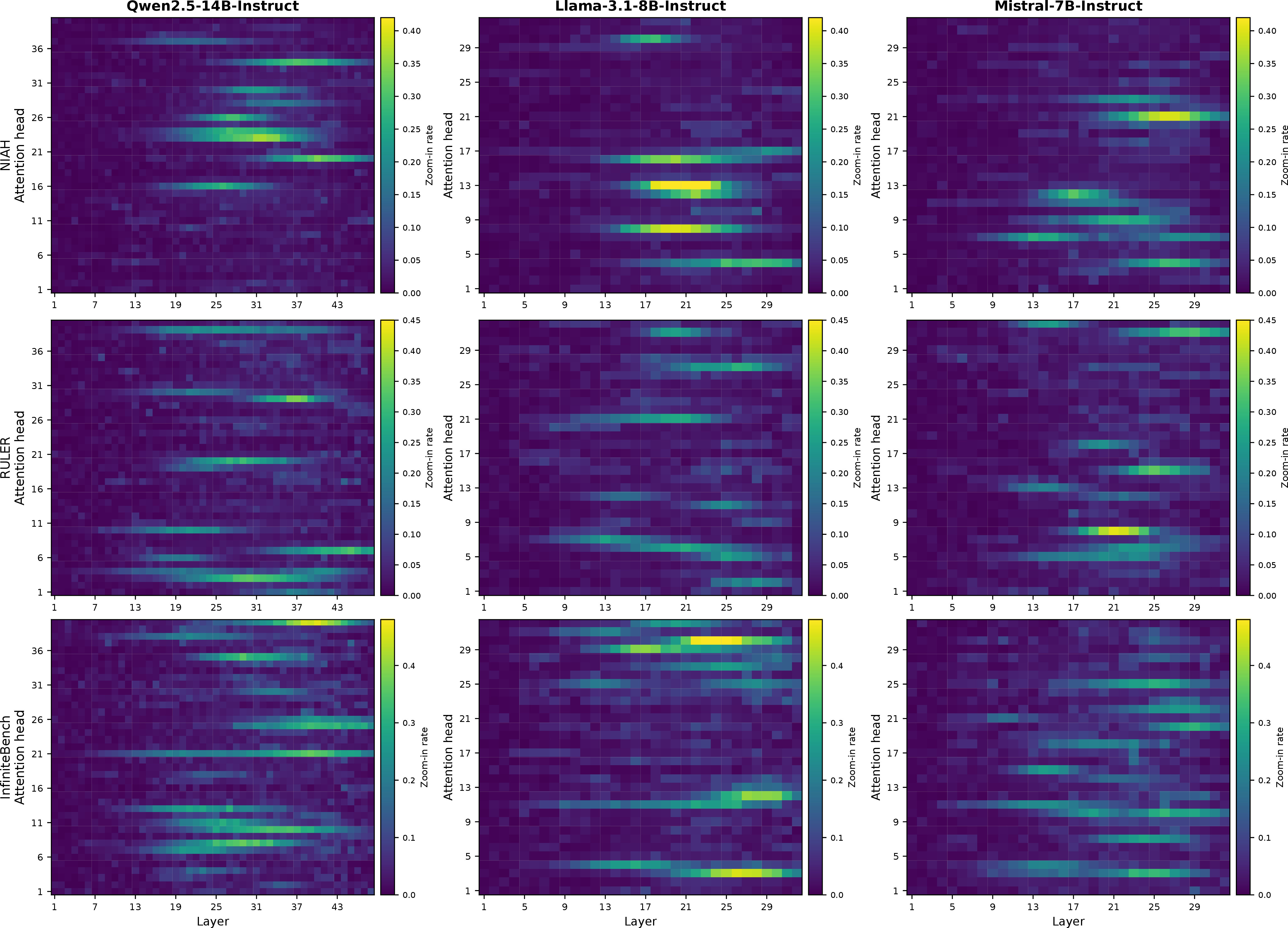
Figure 6 provides additional zoom-in behavior visualizations for SeKV across three backbone models and three long-context benchmarks. Each heatmap reports the average zoom-in rate across layers and attention heads, where brighter regions correspond to heads that more frequently trigger token-level reconstruction. The rows correspond to NIAH, RULER, and InfiniteBench, while the columns correspond to Qwen2.5-14B-Instruct, Llama-3.1-8B-Instruct, and Mistral-7B-Instruct.
The heatmaps show three consistent trends. First, zoom-in is sparse: most heads remain dark across most layers, indicating that SeKV does not uniformly expand compressed spans during decoding. Second, higher zoom-in rates are concentrated in a limited number of heads, suggesting that only a subset of attention heads specialize in long-range evidence recovery. Third, zoom-in activity is generally stronger in middle and later layers, where long-range retrieval and semantic integration are more likely to occur. These observations support the design of learned per-head per-layer thresholds. A single global threshold would either over-expand spans for mostly local heads or under-expand spans for retrieval-oriented heads, which is consistent with the performance drop observed in the fixed-threshold ablation in Table 5.
The benchmark-level differences also align with the nature of each task. NIAH produces sparse but sharp zoom-in patterns because the task requires recovering a specific inserted fact. RULER induces a broader routing pattern because it contains multiple controlled retrieval and reasoning tasks. InfiniteBench shows the most distributed zoom-in behavior, reflecting its longer and more heterogeneous inputs. Overall, these visualizations confirm that SeKV allocates token-level resolution adaptively: it preserves efficiency by leaving most spans compressed, while selectively reconstructing the spans most relevant to the current decoding state.
References↩︎
Corresponding author:
aabaskoh@cs.ubc.ca. Part of this work was done during the internship at Microsoft Research (MSR), Vancouver Lab.↩︎