Quantum Derivative Pricing for SPDEs via BDSDE Representation
January 01, 1970
Abstract
We study quantum speedups of derivative pricing for stochastic partial differential equation (SPDE) models through their backward doubly stochastic differential equation (BDSDE) representations. We develop conditional and nested quantum-accelerated multilevel Monte Carlo (QA-MLMC) methods for estimating the resulting conditional and nested expectations, improving the sampling complexity of classical Monte Carlo methods from \(\widetilde{\mathcal{O}}(\epsilon^{-2})\) to \(\widetilde{\mathcal{O}}(\epsilon^{-1})\) within additive error \(\epsilon\). We apply the framework to derivative pricing and sensitivity analysis, providing quantum-accelerated estimators for prices as well as first-order and second-order Greeks, likelihood-ratio and Malliavin-weight representations for Greeks, and Heston-type stochastic-volatility models. To enable efficient multilevel coupling, we construct a family of Forward–Backward Taylor discretization schemes for the stochastic integrals arising in the BDSDE representations and establish global strong-error order one convergence for pricing and Greek estimators. Numerical experiments showcase our schemes for first-order and second-order Greeks can reach the required orders for the full quadratic quantum speedups.
1 Introduction↩︎
Volatility in modern financial markets is neither constant nor exogenous. It evolves randomly across multiple time scales and interacts with other sources of uncertainty, including liquidity conditions, interest rates, and latent risk factors. Under the classical Black–Scholes framework and its stochastic-volatility extensions, derivative prices can be characterized as solutions of partial differential equations (PDEs) [1]–[3].
When the market environment itself evolves randomly, the pricing operator becomes stochastic, leading naturally to stochastic partial differential equations (SPDEs). Such SPDE formulations arise in a variety of financial settings, including stochastic volatility surface models [4], stochastic term-structure models [5]–[7], and stochastic forward-curve models in energy markets [8]. In these applications, the solution of the SPDE typically represents the value of a contingent claim under a random market environment. Beyond computing option prices, practical applications require the estimation of risk sensitivities, commonly known as Greeks, including Delta, Vega, Gamma, and higher-order parameter sensitivities. These quantities play a central role in dynamic hedging, model calibration, risk management, and uncertainty quantification [9].
The numerical approximation of SPDEs has been studied extensively over the past several decades [10], [11]. A wide range of deterministic and stochastic discretization techniques have been developed, including finite-difference methods, finite-element methods, spectral methods, and stochastic Galerkin approaches [12]–[14]. These methods have achieved considerable success in the simulation and analysis of stochastic systems arising in physics, engineering, and finance.
However, the direct numerical treatment of financial SPDEs remains challenging. In multi-factor stochastic-volatility and term-structure models, the effective state dimension can grow rapidly. As a consequence, grid-based discretizations often suffer from the curse of dimensionality, resulting in substantial computational costs for both spatial discretization and the solution of large-scale linear systems [15], [16].
Moreover, many quantities of practical interest, including option prices, risk measures, and Greek sensitivities, are naturally expressed as expectations or nested expectations of the underlying stochastic system. Accurate estimation of such quantities often requires substantial sampling effort in addition to the numerical solution of the SPDE itself.
These challenges motivate the search for alternative formulations that avoid direct discretization of the underlying SPDE. An attractive approach is provided by probabilistic representations, which reformulate the problem in terms of stochastic differential equations and expectation estimation.
A major development in this direction was the introduction of backward stochastic differential equations (BSDEs) by Pardoux and Peng [17]. BSDEs provide a nonlinear extension of the classical Feynman–Kac formula and establish a probabilistic representation for broad classes of semilinear parabolic PDEs [18], [19]. Since their introduction, BSDEs have become an important tool in stochastic control [20], [21], mathematical finance [22], and nonlinear expectation theory [23], [24].
To extend the probabilistic correspondence between BSDEs and PDEs to stochastic partial differential equations, Pardoux and Peng introduced backward doubly stochastic differential equations (BDSDEs) [25]. They established a stochastic Feynman–Kac formula showing that solutions of a broad class of quasilinear SPDEs can be represented by solutions of BDSDEs driven simultaneously by a forward Brownian motion and a backward Brownian motion. For the class of stochastic option-pricing SPDEs considered in this work, let \(X^{t,x}\) denote the forward state process describing the underlying risk factors, initialized from \(x\) at time \(t\). Then the SPDE solution admits a BDSDE representation of the form \[\begin{align} u(s,X_s^{t,x})=Y_s^{t,x},\quad X_t^{t,x}=x, \quad s\in[t,T], \end{align}\] where \(Y_s^{t,x}\) solves the associated BDSDE. This representation transforms the original SPDE problem into the estimation of stochastic expectations and avoids direct spatial discretization of the underlying equation. Moreover, the coexistence of forward and backward sources of randomness naturally leads to conditional and nested expectation structures, providing a probabilistic foundation for Monte Carlo, multilevel Monte Carlo, and quantum mean estimation methodologies.
The numerical solution of BSDEs and BDSDEs has attracted considerable attention over the past several decades. For BSDEs, a variety of time-discretization, regression-based, and Monte Carlo methods have been developed [26]–[28]. These approaches provide practical algorithms for approximating BSDE solutions and have led to a rich literature on numerical methods for high-dimensional PDEs through probabilistic representations. More recently, BSDE formulations have inspired a variety of machine-learning approaches for high-dimensional PDEs, including Deep BSDE methods, deep backward dynamic programming schemes, and related neural-network-based algorithms [29]–[31]. These methods substantially improve scalability in high-dimensional settings and have become an active research direction at the interface of scientific computing and machine learning.
For BDSDEs, several numerical approximation schemes have been proposed, including Euler-type and regression-based methods [32], [33]. In particular, [34] developed a first-order scheme based on a two-sided Itô–Taylor expansion. Since many of these schemes rely on conditional expectations with respect to the forward Brownian motion, the forward randomness is integrated out at each time step. As a consequence, they do not directly provide the pathwise strong approximations required for multilevel Monte Carlo coupling and Greek estimation.
Many quantities arising from BDSDE representations, including option prices and Greek sensitivities, are naturally expressed as stochastic expectations. To estimate such quantities efficiently, multilevel Monte Carlo (MLMC), introduced by Giles [35], exploits strong couplings between successive discretization levels to achieve substantial computational savings over standard Monte Carlo methods.
MLMC has been successfully applied to a wide range of problems in computational finance, including Greek estimation, efficient risk measurement, and basket option pricing [36]–[39]. It has also been extended to stochastic partial differential equations [40]–[42]. In particular, [43] developed a multilevel Monte Carlo framework based on a Milstein finite difference discretization for SPDEs and demonstrated its effectiveness in the pricing of basket credit derivatives. To the best of our knowledge, however, the combination of MLMC and BDSDE representations has received little attention in the existing literature.
Recent advances in quantum computing have opened new possibilities for further accelerating stochastic simulation. Quantum amplitude estimation and related quantum mean estimation algorithms reduce the sampling complexity of expectation estimation from \(\mathcal{O}(\epsilon^{-2})\) to \(\widetilde{\mathcal{O}}(\epsilon^{-1})\), thereby providing a quadratic speedup over classical Monte Carlo methods [44]–[47]. Building on these developments, quantum-accelerated multilevel Monte Carlo (QA-MLMC) methods have recently emerged as a powerful framework for expectation estimation. [48] combined quantum mean estimation with MLMC and established quantum speedups for stochastic differential equations. Subsequent developments further extended and refined this framework, including quadratic speedups for nonlinear and nested expectation problems and related stochastic simulation tasks [49]–[52].
At the same time, quantum algorithms have also been investigated for financial PDEs and derivative pricing. Examples include quantum algorithms for option valuation and financial simulation [53]–[55], as well as recent end-to-end quantum PDE frameworks for option pricing under Black–Scholes and Heston-type models [56]. These works demonstrate the potential of quantum computation for high-dimensional problems arising in quantitative finance. On the other hand, quantum algorithms have also been explored for the numerical solution of BSDEs. For example, [57] introduced a quantum least-squares Monte Carlo approach for solving BSDEs.
However, most existing quantum approaches mainly focus on PDEs, SDEs, or BSDEs. To the best of our knowledge, although quantum simulation algorithms for stochastic differential equations are recently studied [58]–[62], quantum algorithms for SPDEs based on BDSDE representations have not yet been systematically studied. The extension of these ideas to SPDEs faces several challenges.
A key difficulty is that achieving the optimal complexity \(\widetilde{\mathcal{O}}(\epsilon^{-1})\) requires not only quantum acceleration, but also effective multilevel coupling and sufficiently accurate pathwise discretizations. In the standard multilevel complexity analysis, if the bias, variance, and cost exponents are denoted by \((\alpha,\beta,\gamma)\), then achieving the optimal quantum complexity typically requires \[\beta\ge 2\gamma,\] which is stronger than the classical MLMC requirement \(\beta\ge\gamma\). Equivalently, if a discretization has strong convergence order \(r\) so that the level-difference variance behaves like \(\mathcal{O}(h^{2r})\), then the optimal QA-MLMC regime requires \[r=\frac{\beta}{2}\ge \gamma.\] For direct discretizations of a \(d\)-dimensional SPDE, the cost exponent \(\gamma\) is often large because each sample involves the spatial degrees of freedom of the discretized random field. For instance, if a tensor-product grid with mesh size \(h_\ell\) is used in each spatial coordinate and the cost per grid point is uniformly bounded, then the number of spatial grid points is proportional to \(h_\ell^{-d}\). Hence \(\gamma_{\mathrm{SPDE}} = d\). Thus, achieving the optimal QA-MLMC complexity would require a strong approximation order comparable to the spatial dimension (\(r\ge \gamma_{\mathrm{SPDE}}= d\)), which is generally unrealistic in high-dimensional settings.
Even after passing to a BDSDE formulation, a standard strong-error order-\(1/2\) discretization (e.g., Euler discretization) is still insufficient for the full quantum speedup. When \(\gamma=1\) and \(r=1/2\), the variance exponent is only \(\beta=1\), and the resulting QA-MLMC complexity is typically \(\widetilde{\mathcal{O}}(\epsilon^{-3/2})\) rather than \(\widetilde{\mathcal{O}}(\epsilon^{-1})\). This is why the strong-error order one Forward–Backward Taylor discretization developed in this work is essential: it yields \(r=1\), reaching the critical regime \(\beta=2\gamma\) and enabling the full quadratic quantum speedup. The comparison is summarized in Table 1.
| Approach | Cost exponent | Strong-error order | MLMC complexity | QA-MLMC complexity |
|---|---|---|---|---|
| Direct SPDE discretization | \(\gamma_{\mathrm{SPDE}}= d\) | \(r\ge d\) (unrealistic) | \(\widetilde{\mathcal O}(\epsilon^{-2})\) | \(\widetilde{\mathcal O}(\epsilon^{-1})\) |
| Standard BDSDE discretization | \(\gamma_{\mathrm{BDSDE}}=1\) | \(r=\frac12\) | \(\widetilde{\mathcal O}(\epsilon^{-2})\) | \(\widetilde{\mathcal O}(\epsilon^{-3/2})\) |
| Our method (Theorem [thm:QAMLMC32for32u32when32given32B] and Section [sec:sec:Strong-Order-One32Numerical32Schemes32for32Pricing32and32Greek32Estimators]) | \(\gamma_{\mathrm{BDSDE}}=1\) | \(r=1\) | \(\widetilde{\mathcal O}(\epsilon^{-2})\) | \(\widetilde{\mathcal O}(\epsilon^{-1})\) |
These considerations indicate that extending quantum multilevel methods to SPDEs requires more than a direct application of existing QA-MLMC theory.
Existing QA-MLMC frameworks are primarily designed for expectation estimation problems arising from SDE-type path simulations. In contrast, the BDSDE representation of SPDE solutions introduces an additional backward source of randomness, which naturally gives rise to conditional and nested expectation structures. These structures require quantum multilevel estimators that are adapted to the two sources of randomness.
Moreover, most existing multilevel and quantum approaches in this area focus primarily on pricing problems. By contrast, efficient estimators for first- and second-order Greeks under stochastic-environment models are much less developed. This leaves open the construction of multilevel and quantum estimators for sensitivity analysis in the SPDE and BDSDE setting.
1.1 Contributions↩︎
In this work, we develop a unified computational framework for stochastic derivative-pricing SPDEs based on their BDSDE representations. The framework combines multilevel Monte Carlo, conditional and nested quantum estimators, and new Forward–Backward
Taylor discretization schemes with strong-error order one convergence, allowing derivative pricing and Greek estimation to be treated within a common probabilistic setting.
1.1.0.1 Modeling and algorithms.
BDSDE-based framework for SPDE pricing and sensitivity analysis.
Section 2 introduces the SPDE models arising in stochastic-environment financial markets and develops a BDSDE-based probabilistic representation. This representation reformulates pricing and Greek estimation problems as conditional and nested expectation estimation tasks, providing a unified framework for direct pricing, first-order sensitivities, and second-order sensitivities. The resulting estimation framework serves as the foundation for all subsequent quantum algorithms developed in this work.
Conditional quantum-accelerated multilevel Monte Carlo for SPDEs.
Building on the BDSDE-based estimation framework, we develop a conditional QA-MLMC methodology for approximating \[\begin{align} u(t,x;B) =\mathbb{E}_W[P(t,x;B)\mid B]. \end{align}\] The key ingredients are the conditional quantum level-\(\ell\) difference evaluator (Algorithm 1), which constructs quantum estimators for the level differences appearing in the multilevel decomposition, and the conditional quantum-accelerated MLMC estimator \(\widehat{u}(t,x;B)\) (Algorithm 2), which combines these level differences across discretization levels to produce a complete conditional estimator of \(u(t,x;B)\).
Nested quantum-accelerated multilevel Monte Carlo for SPDEs.
Building on recent quantum algorithms for nonlinear and nested expectation estimation [50], [63], we specialize the nested QA-MLMC framework to the BDSDE representations arising from SPDEs. This yields a nested quantum-accelerated estimator (Algorithm 4) for quantities of the form \[\begin{align} \mathbb{E}_B\!\left[\varphi(u(t,x;B))\right]. \end{align}\] The resulting methodology combines the coupled level difference evaluator (Algorithm 3) with a nested multilevel quantum estimation procedure, thereby extending quantum multilevel techniques to nested expectation structures arising naturally in stochastic-environment SPDE models.
Applications to derivative pricing and sensitivity analysis.
In Section 4, we specialize the conditional and nested QA-MLMC frameworks to derivative pricing and sensitivity analysis. Using the probabilistic representations developed in this work, we construct quantum estimators for a broad class of first-order Greeks, including Delta, spot Vega, Rho, and general parameter Greeks; smooth second-order Greeks like Gamma, Vanna and Volga; extensions to nonsmooth payoffs via likelihood-ratio and Malliavin-weight representations; and Heston-type stochastic-volatility models.
Global strong-error order one analysis and numerical experiments.
In Section 5, we establish a global strong-error framework for the BDSDE payoff functionals arising in pricing, first-order Greek estimation, and second-order Greek estimation. We then construct concrete Forward–Backward Taylor discretization operators and prove that they satisfy the first-order consistency and accumulated stability properties required by this framework. Consequently, the resulting estimators achieve global strong convergence of order one.
We further validate this theory through numerical experiments in Section 6. For pricing, first-order Greek estimation, and second-order Greek estimation, the observed multilevel exponents satisfy \[(\alpha,\beta,\gamma)\approx(1,2,1),\] confirming the strong-error order one behavior predicted by the theory and the conditions required for the quadratic quantum speedup.
1.1.0.2 Theorems.
BDSDE representation and QA-MLMC foundations.
Theorem 1, following [25], [64], provides the BDSDE representation for a class of linear backward SPDEs and serves as the probabilistic foundation of our framework. Theorem 2, following [48], recalls the general quantum-accelerated MLMC methodology that underlies our quantum complexity analysis.
Conditional quantum speedups for SPDE solution estimation.
Theorem 3 shows that, conditioned on a realization of the environmental Brownian motion \(B\), the SPDE solution \[\begin{align} u(t,x;B)=\mathbb{E}_W[P(t,x;B)\mid B] \end{align}\] can be estimated with additive error \(\epsilon\) using computational cost \[\begin{align} \widetilde{\mathcal{O}}(\epsilon^{-1}), \end{align}\] yielding a quadratic quantum speedup over classical Monte Carlo methods.
Quantum speedups for nested SPDE expectations.
Theorem 4 extends the conditional framework to nested quantities of the form \[\begin{align} \mathbb{E}_B[\varphi(u(t,x;B))]. \end{align}\]
Under suitable regularity and moment assumptions, the resulting nested QA-MLMC estimator achieves additive error \(\epsilon\) with overall complexity \[\begin{align} \widetilde{\mathcal{O}}(\epsilon^{-1}), \end{align}\] thereby extending quantum speedups to SPDE quantities involving both forward and backward randomness.
Quantum estimation of first and second-order Greeks.
Propositions 1 and 2 derive pathwise conditional representations for first-order and second-order Greeks. These representations express the Greeks as conditional expectations of explicitly constructed payoff functionals involving first-order and second-order variational processes.
Building on these representations, Corollaries 1 and 2 show that both conditional and unconditional Greeks can be estimated with additive error \(\epsilon\) using quantum-accelerated MLMC methods with complexity \[\begin{align} \widetilde{\mathcal{O}}(\epsilon^{-1}). \end{align}\]
Global strong-error order one schemes via Forward–Backward Taylor discretization.
Proposition 3, Proposition 6, and Proposition 9 establish a general strong-error framework showing that global strong-error order one follows whenever the constituent discretization operators satisfy suitable first-order consistency and stability properties.
To realize this framework, we introduce a new family of Forward–Backward Taylor discretization schemes for the stochastic integrals arising in the BDSDE representations of pricing and Greek estimators. The construction explicitly captures mixed forward–backward iterated integrals and provides concrete discretization operators for pricing, first-order Greeks, and second-order Greeks.
Propositions 4, 5, 7, 8, 10, and 11 verify that the Forward–Backward Taylor discretization satisfies the required strong-error order one consistency and stability conditions. Consequently, all resulting pricing and Greek estimators achieve global strong convergence of order one.
1.2 Organization↩︎
Section 1 introduces the background and motivation of the work, reviews the related literature, and summarizes the main contributions.
Section 2 presents the SPDE models considered in this paper and develops the BDSDE-based probabilistic representation and estimation framework that serves as the foundation of our methodology.
Section 3 develops the quantum-accelerated multilevel Monte Carlo framework. Subsection 3.1 introduces the conditional QA-MLMC estimator for approximating \(u(t,x;B)=\mathbb{E}_W[P(t,x;B)\mid B]\), while Subsection 3.2 develops the nested QA-MLMC estimator for quantities of the form \(\mathbb{E}_B[\varphi(u(t,x;B))]\).
Section 4 specializes the general framework to derivative pricing and sensitivity analysis. We derive conditional pricing representations, first- and second-order Greek representations, and the corresponding conditional and nested quantum estimators. Several extensions, including nonsmooth payoffs and Heston-type stochastic-volatility models, are also discussed.
Section 5 contains the main numerical analysis component of the paper. We develop strong-error order one numerical schemes for pricing and Greek estimators and establish the strong-convergence and stability results required for the quantum-accelerated multilevel complexity analysis.
Section 6 presents numerical experiments validating the proposed Forward–Backward Taylor discretization and the multilevel convergence properties across multiple realizations of the backward Brownian motion.
Finally, Section 7 concludes the paper by summarizing the main contributions and outlining possible directions for future work.
The appendices contain additional background material and technical proofs. In particular, Appendix 8 reviews the classical BDSDE representation of SPDEs, while Appendix 9 contains the proofs of the strong-error framework and the numerical analysis results developed in Section 5.
2 SPDE Formulation and Probabilistic Representation↩︎
2.1 From Stochastic Volatility Models to SPDEs↩︎
We begin with the classical Heston stochastic model [2] under the risk-neutral measure: \[\begin{align} \tag{1} \mathrm dS_t&=rS_t\,\mathrm dt+ \sqrt{V_t}\,S_t\,\mathrm dW_t^{(S)},\\ \tag{2} \mathrm dV_t&=\kappa(\theta-V_t)\,\mathrm dt +\xi\sqrt{V_t}\,\mathrm dW_t^{(V)}, \end{align}\] where \(S_t\) denotes the asset price, \(V_t\) is the instantaneous variance process, \(r\) is the risk-free interest rate, \(\kappa\) is the mean-reversion rate, \(\theta\) is the long-run variance level, \(\xi\) is the volatility-of-volatility parameter, and \[\begin{align} \label{eq:Heston32cor} \mathrm d\langle W^{(S)},W^{(V)}\rangle_t =\rho\,\mathrm dt. \end{align}\tag{3}\]
For a European payoff \(g(S_T)\), the option price is \[\begin{align} u(t,s,v) =\mathbb{E}^{\mathbb{Q}} \left[e^{-r(T-t)}g(S_T) \mid S_t=s,\,V_t=v \right]. \end{align}\]
Under standard regularity assumptions, the standard arbitrage-free pricing arguments [1], [65] imply that the option price \(u(t,s,v)\) satisfies the partial differential equation (PDE) \[\begin{align} \partial_t u+\mathcal{L} u-r u=0, \end{align}\] with terminal condition \[u(T,s,v)=g(s),\] where the generator \(\mathcal{L}\) associated with 1 –3 is given by \[\begin{align} \mathcal{L} =rs\partial_s +\kappa(\theta-v)\partial_v +\frac{1}{2} vs^2\partial_{ss} +\rho\xi sv\,\partial_{sv} +\frac{1}{2}\xi^2v\,\partial_{vv}. \end{align}\]
The above pricing equation is deterministic because all market factors are assumed to be either deterministic or fully represented by the finite-dimensional state variables \((S_t,V_t)\).
In modern financial markets, however, quantities such as volatility surfaces, liquidity conditions, interest-rate environments, and latent risk factors may themselves evolve randomly over time. As a consequence, the coefficients of the pricing equation become random, and the option value must be viewed as a random field.
Motivated by this observation, we consider stochastic option-pricing SPDEs of the form \[\begin{align} \label{eq:spde0} \mathrm du=\bigl(\mathcal{L} u -r u+F\bigr)\,\mathrm dt+G\,\mathrm dB_t, \end{align}\tag{4}\] with terminal condition \[\begin{align} u(T,s,v)=g(s). \end{align}\] Here, \(\mathcal{L}\) denotes the stochastic-volatility generator, \(r\) is the discount rate, \(F\) is a source term, and \(G\) characterizes the stochastic forcing induced by the random market environment.
Direct numerical discretization of 4 is computationally demanding, particularly in high-dimensional settings. To facilitate efficient numerical approximation, we employ a probabilistic representation based on backward doubly stochastic differential equations (BDSDEs). This representation transforms the SPDE problem into the estimation of conditional expectations over stochastic paths and serves as the foundation of the algorithms developed in this paper.
2.2 BDSDE Representation and Estimation Framework↩︎
A key advantage of stochastic partial differential equations is that, under suitable regularity conditions, their solutions admit probabilistic representations through backward doubly stochastic differential equations (BDSDEs). Introduced by Pardoux and Peng [25], BDSDEs extend the classical Feynman–Kac formula and provide a probabilistic representation for a broad class of quasilinear SPDEs.
In this work, the SPDE is treated through its associated BDSDE representation. Since the SPDE–BDSDE correspondence is classical, we only summarize the formulation required for the subsequent numerical analysis. Further details can be found in Appendix 8.
In our applications, we are primarily interested in the linear setting. Following [64], we consider the following class of linear backward SPDEs.
Theorem 1. For the linear backward SPDE \[\label{eq:linear32SPDE40with32BDSDE410} \begin{cases} \mathrm{d} u(t,x) = \Bigl[\mathcal{L}u(t,x) + F(t,x) + c(t)u(t,x) + \widetilde{c}(t)(\sigma^\top\nabla u)(t,x)\Bigr]\,\mathrm{d}t + \Bigl[H(t,x)+d(t)u(t,x)\Bigr]\,\mathrm{d}B_t,\quad t\in[0,T],\\ u(T,x)=G(x), \end{cases}\qquad{(1)}\] where \(u:\mathbb{R_+}\times \mathbb{R}^d\rightarrow \mathbb{R}^k\) and \(\mathcal{L}u=\left( Lu_1,\cdots ,Lu_k \right)^\top\) with \(L=\frac{1}{2}\sum\limits_{i,j=1}^d(\sigma\sigma^\top)_{ij}\frac{\partial^2}{\partial x_i\partial x_j}+\sum\limits_{i=1}^db_i\frac{\partial}{\partial x_i}.\) Assume that \(G\in C_p^3(\mathbb{R}^d)\), \(F, H\in C_b^3([0,T]\times\mathbb{R}^d)\) and \(c,\widetilde{c},d\) are bounded deterministic functions. Let \(\{X_s^{t,x};t\leq s\leq T\}\) be the solution of the SDE \[\label{eq:SDE40with32BDSDE410} \begin{cases} \mathrm{d}X_s^{t,x}=b(X_s^{t,x})\,\mathrm{d}s +\sigma(X_s^{t,x})\,\mathrm{d}W_s,\quad s\in[t,T],\\ X_t^{t,x}=x. \end{cases}\qquad{(2)}\] Define the stochastic exponential \(\Phi(s,r)\) as \[\begin{align} \Phi(s,\tau)=\exp\left(\int_s^\tau c(r)\,\mathrm{d}r +\int_s^\tau d(r)\mathrm d \overleftarrow{B}_r +\int_s^\tau \widetilde{c}(r)\,\mathrm{d}W_r -\frac{1}{2}\int_s^\tau\left(|\widetilde{c}(r)|^2-|d(r)|^2\right)\,\mathrm{d}r\right). \end{align}\] Then the SPDE ?? has a unique solution and it can be written as \[\begin{align} \label{eq:u40t44x410} u(t,x)=\mathbb{E}\left[\Phi(t,T)G(X_T^{t,x}) +\int_t^T\Phi(t,r)\left(F(r,X_r^{t,x})+d(r) H(r,X_r^{t,x})\right)\,\mathrm{d}r +\int_t^T\Phi(t,r)H(r,X_r^{t,x})\mathrm d \overleftarrow{B}_r\,|\,\mathcal{F}_{t,T}^B \right]. \end{align}\qquad{(3)}\] For convenience in the subsequent discussion, when the Brownian motion \(B\) is fixed, we denote \[\begin{align} \label{eq:eq32of32P40t44x59B41} P(t,x;B)=\Phi(t,T)G(X_T^{t,x}) +\int_t^T\Phi(t,r)\left(F(r,X_r^{t,x})+d(r) H(r,X_r^{t,x})\right)\,\mathrm{d}r +\int_t^T\Phi(t,r)H(r,X_r^{t,x})\mathrm d \overleftarrow{B}_r \end{align}\qquad{(4)}\] and \[\begin{align} \label{eq:u(t,x;B)=E[P]} u(t,x;B)=\mathbb{E}_W[P(t,x;B)]. \end{align}\qquad{(5)}\]
Remark 1. Here, the quantity \(P\) depends on the solution of the SDE \(X_r^{t,x}\), and the expectation is taken with respect to the randomness arising from the SDE.
Theorem 1 reduces the solution of the SPDE to the evaluation of a path functional \(P(t,x;B)\). For a fixed realization of the backward Brownian motion \(B\), the only remaining randomness in ?? comes from the forward Brownian motion \(W\). Consequently, the SPDE solution admits the conditional expectation representation \[\begin{align} u(t,x;B) =\mathbb{E}_W \bigl[P(t,x;B)\,\big|\,B\bigr]. \end{align}\] This observation transforms the original SPDE problem into the estimation of a conditional expectation with respect to the forward diffusion.
In many applications, the quantity of ultimate interest is obtained after averaging over the random environment generated by \(B\). This leads to the nested expectation \[\begin{align} U(t,x) =\mathbb{E}_B \bigl[u(t,x;B)\bigr] =\mathbb{E}_B \Big[\mathbb{E}_W \bigl[P(t,x;B)\,\big|\,B\bigr]\Big]. \end{align}\]
Consequently, the probabilistic representation naturally gives rise to two estimation problems. The first is the conditional estimation problem \[\begin{align} u(t,x;B) =\mathbb{E}_W \bigl[P(t,x;B)\,\big|\,B\bigr], \end{align}\] where the realization of \(B\) is fixed. The second is the nested estimation problem \[\begin{align} U(t,x) =\mathbb{E}_B \bigl[u(t,x;B)\bigr], \end{align}\] which requires averaging over both sources of randomness.
These two estimation problems form the basis of the multilevel Monte Carlo and quantum algorithms developed in the subsequent sections.
3 Quantum-accelerated MLMC for SPDEs↩︎
The probabilistic representation developed in the previous section reduces the SPDE problem to the estimation of conditional and nested expectations associated with the path functional \(P(t,x;B)\). To estimate efficiently, we employ multilevel Monte Carlo (MLMC) together with quantum mean estimation.
Suppose that a sequence of approximations \(\{\Phi_\ell\}_{\ell\ge0}\) to a random variable \(\Phi\) is available and satisfies \[\begin{align} \left|\mathbb{E}[\Phi]-\mathbb{E}[\Phi_\ell]\right|=\mathcal{O}(2^{-\alpha\ell}), \quad \operatorname{Var}(\Phi_\ell-\Phi_{\ell-1}) =\mathcal{O}(2^{-\beta\ell}), \quad \operatorname{Cost}(\Phi_\ell) =\mathcal{O}(2^{\gamma\ell}), \end{align}\] for some \(\alpha,\beta,\gamma>0\). The MLMC estimator is based on the telescoping identity \[\begin{align} \mathbb{E}[\Phi_L]=\mathbb{E}[\Phi_0] +\sum_{\ell=1}^{L}\mathbb{E}[\Phi_\ell-\Phi_{\ell-1}]. \end{align}\] Under the standard MLMC framework [35], [66], if \(\beta>\gamma\), an estimator with mean-square error \(\mathcal{O}(\epsilon^2)\) can be constructed with overall computational complexity \(\mathcal{O}(\epsilon^{-2})\).
Recent advances in quantum computing provide the possibility of further accelerating expectation estimation. In particular, quantum mean estimation algorithms reduce the sampling complexity from \(\mathcal{O}(\epsilon^{-2})\) to \(\widetilde{\mathcal{O}}(\epsilon^{-1})\), yielding a quadratic speedup over classical Monte Carlo methods. The following result will be used as the basic quantum subroutine.
Lemma 1 (Quantum mean estimation [47]). Suppose a random variable \(\Phi\) admits an efficient quantum encoding. Then there exists a quantum algorithm which estimates \(\mathbb{E}[\Phi]\) with additive error \(\sigma(\Phi)/n\) using \(\mathcal{O}(n)\) oracle calls, with constant success probability.
Using the standard powering argument [67], the success probability can be amplified from a constant to \(1-\delta\) with an additional \(\mathcal{O}(\log(1/\delta))\) overhead.
For notational simplicity, we write \[\operatorname{QME}(\Phi;\epsilon,\delta)\] for a quantum mean estimation subroutine which returns an estimate \(\widehat \mu\) of \(\mathbb{E}[\Phi]\) such that \[\Pr\left( |\widehat\mu-\mathbb{E}[\Phi]|\le \epsilon \right) \ge 1-\delta .\]
Replacing the classical sample average on each MLMC level by QME leads to quantum-accelerated MLMC (QA-MLMC). Our algorithm is mainly based on the following quantum-accelerated Monte Carlo methods proposed in [48].
Theorem 2. Let \(\Phi\) be a random variable, and let \(\Phi_\ell~(\ell=0,1,\ldots,L)\) be a sequence of random variables approximating \(\Phi\) at level \(\ell\). Further define \(\Phi_{-1}=0\). Let \(C_\ell\) be the cost of sampling from \(\Phi_\ell\), and let \(V_\ell\) be the variance of \(\Phi_\ell-\Phi_{\ell-1}\). If there exist positive constants \(\alpha, \beta,\gamma\) such that \[\begin{align} & \begin{cases} |\mathbb{E}[\Phi_\ell-\Phi]| = \mathcal{O}(2^{-\alpha \ell}),\\ V_\ell = \mathcal{O}(2^{-\beta \ell}),\\ C_\ell = \mathcal{O}(2^{\gamma \ell}) \end{cases} && \end{align}\] Then for any \(\epsilon< 1/e\) there is a quantum algorithm that estimates \(\mathbb{E}[\Phi]\) up to additive error \(\epsilon\) with probability at least 0.99, and with cost \[\begin{align} \begin{cases} \widetilde{\mathcal{O}}\left(\epsilon^{-1}\right), & \beta \geq 2\gamma, \\ \widetilde{\mathcal{O}}\left(\epsilon^{-1 - (\gamma - 0.5\beta)/\alpha}\right), & \beta < 2\gamma. \end{cases} \end{align}\]
However, the complexity requirements for QA-MLMC are substantially more restrictive. In particular, achieving the optimal quantum complexity \(\widetilde{\mathcal{O}}(\epsilon^{-1})\) requires \(\beta\ge 2\gamma\), which is stronger than the classical MLMC requirement \(\beta\ge\gamma\). For discretization-based SPDE solvers, the cost exponent \(\gamma\) is often large due to the curse of dimensionality. For example, under standard tensor-product spatial discretizations of a \(d\)-dimensional SPDE, one typically has \(\gamma\approx d.\) Since the MLMC variance exponent typically satisfies \(\beta=2r\), where \(r\) is the strong convergence order, the condition \(\beta\ge2\gamma\) would require \(r\ge d,\) namely, a strong convergence order at least equal to the spatial dimension, which is generally unrealistic in practice.
The BDSDE representation developed in the previous section avoids direct spatial discretization of the SPDE and converts the problem into the estimation of stochastic path functionals. This structure enables the construction of efficient multilevel estimators with favorable variance decay properties and provides a natural foundation for quantum acceleration.
In the remainder of this section, we first consider the conditional estimation problem and then extend the framework to the nested setting.
3.1 Conditional Quantum-accelerated MLMC Estimator↩︎
The probabilistic representation introduced in Subsection 2.2 reduces the pricing problem to the estimation of the conditional expectation \[\begin{align} u(t,x;B) =\mathbb{E}_W[P(t,x;B)\mid B]. \end{align}\] To construct the conditional quantum-accelerated estimators, we first develop suitable discretizations for the stochastic quantities appearing in this representation. Recalling that \[\begin{align} P(t,x;B) =\Phi(t,T)G(X_T^{t,x}) +\int_t^T\Phi(t,r)\left(F(r,X_r^{t,x})+d(r) H(r,X_r^{t,x})\right)\,\mathrm{d}r +\int_t^T\Phi(t,r)H(r,X_r^{t,x})\mathrm d \overleftarrow{B}_r, \end{align}\] we observe that there are three components that require discretization: the evolution of the SDE, the exponential weight \(\Phi\), and the integrals over the time interval \([t,T]\).
In classical numerical schemes, these components are often discretized using Euler-type methods, which already provide sufficient accuracy. However, in quantum algorithms, higher-order convergence is often required. Therefore, we introduce a unified notation \(\mathcal{S}\) to denote the discretization operators associated with each component, allowing us to systematically track and analyze their respective convergence properties.
We introduce three discretization operators. Let \[\begin{align} \Delta W_k:=W_{t_{k+1}}-W_{t_k}, \quad \Delta\overleftarrow B_k:=B_{t_k}-B_{t_{k+1}}, \quad t_k=t+kh . \end{align}\]
(1) State discretization \(\mathcal{S}_X\). Given the current state \(X_k\), the time \(t_k\), the stepsize \(h\), and the forward Brownian increment \(\Delta W_k\), we set \[\begin{align} \label{eq:def32of32S95X} X_{k+1}=\mathcal{S}_X(X_k,t_k,h;\Delta W_k). \end{align}\tag{5}\]
(2) Exponential weight discretization \(\mathcal{S}_\Phi\). Given the current weight \(\Phi_k\), the time \(t_k\), the stepsize \(h\), the forward Brownian increment \(\Delta W_k\), and the backward Brownian increment \(\Delta\overleftarrow B_k\), we set \[\begin{align} \label{eq:def32of32S95phi} \Phi_{k+1}=\mathcal{S}_\Phi(\Phi_k,t_k,h; \Delta W_k,\Delta\overleftarrow B_k). \end{align}\tag{6}\]
(3) Integral discretization \(\mathcal{S}_{\mathrm{int}}\). Given the current term \(Y_k\), weight \(\Phi_k\), state \(x_k\), the time \(t_k\), the stepsize \(h\), and the Brownian increments \((\Delta W_k,\Delta\overleftarrow B_k)\), we set \[\begin{align} \label{eq:def32of32S95int} Y_{k+1}=Y_k+ \mathcal{S}_{\mathrm{int}}\left( \Phi_k,x_k,t_k,h; \Delta W_k,\Delta\overleftarrow B_k \right). \end{align}\tag{7}\]
Assume that reversible unitary implementations of the discretization operators \(\mathcal{S}_X,\mathcal{S}_\Phi\) and \(\mathcal{S}_{\mathrm{int}}\) are available in the following standard form: \[\begin{align} O_X &: |x,s,h,\Delta W\rangle|0\rangle \mapsto |x,s,h,\Delta W \rangle\ket{\mathcal{S}_X(x,s,h;\Delta W)},\\ O_\Phi &: |\Phi,s,h,\Delta W,\Delta\overleftarrow B\rangle|0\rangle \mapsto |\Phi,s,h,\Delta W,\Delta\overleftarrow B\rangle \ket{\mathcal{S}_\Phi(\Phi,s,h;\Delta W,\Delta\overleftarrow B)},\\ O_\mathrm{int}&: \ket{Y,\Phi,x,s,h;\Delta W,\Delta\overleftarrow B}\ket{0} \mapsto \ket{Y,\Phi,x,s,h;\Delta W,\Delta\overleftarrow B} \ket{Y+\mathcal{S}_\mathrm{int}\left(\Phi,x,s,h;\Delta W,\Delta\overleftarrow B\right)}. \end{align}\]
For notational simplicity, we combine these elementary reversible updates into a single one-step oracle. Suppressing unchanged input registers, work registers, and the standard uncomputation of ancillas, we write, for \(\eta\in\{h,2h\}\), \[\mathcal{U}_{\mathcal{S},\eta}(s;\Delta W,\Delta\overleftarrow B): \ket{X,\Phi,Y} \mapsto \ket{ \mathcal{S}_X(X,s,\eta;\Delta W), \mathcal{S}_\Phi(\Phi,s,\eta;\Delta W,\Delta\overleftarrow B), Y+\mathcal{S}_{\rm int}(\Phi,X,s,\eta;\Delta W,\Delta\overleftarrow B) }.\]
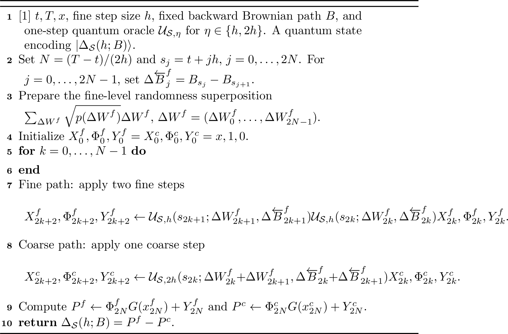
The returned quantum state \(\ket{\Delta_{\mathcal{S}}(h;B)}\) encodes a coupled multilevel difference sample conditioned on \(B\). For notational uniformity, define \[\Delta_0(t,x;B):=P_0(t,x;B), \quad \Delta_\ell(t,x;B) := P_\ell^{f}(t,x;B)-P_{\ell}^{c}(t,x;B), \quad \ell\ge1.\] The fine and coarse trajectories are generated using the shared Brownian coupling \[\Delta W_k^c = \Delta W_{2k}^f+\Delta W_{2k+1}^f, \quad \Delta\overleftarrow B_k^c = \Delta\overleftarrow B_{2k}^f + \Delta\overleftarrow B_{2k+1}^f.\]
For a fixed realization of \(B\), the conditional multilevel identity gives \[u_L(t,x;B) = \mathbb{E}_W[P_L(t,x;B)\mid B] = \sum_{\ell=0}^{L} \mathbb{E}_W[\Delta_\ell(t,x;B)\mid B].\] By Lemma 1, each conditional level mean can be estimated by applying QME to the corresponding quantum encoding.
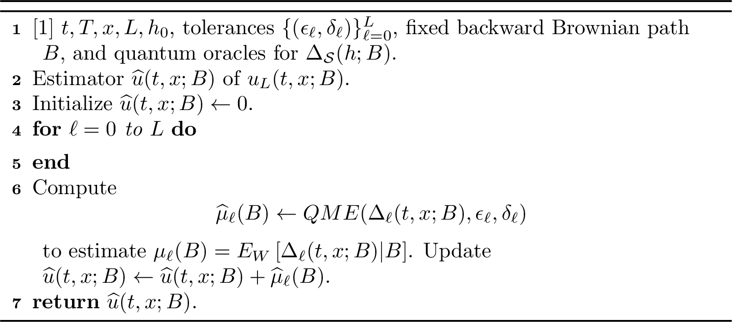
Algorithm 2 combines the conditional multilevel telescoping decomposition with quantum mean estimation applied independently on each level. The resulting estimator approximates the conditional quantity \[u_L(t,x;B) =\mathbb{E}_W[P_L(t,x;B)\mid B].\]
Theorem 3. Assume that:
(1) \(G\in C_p^3(\mathbb{R}^d)\) is globally Lipschitz, \(F,H\in C_b^3([0,T]\times\mathbb{R}^d)\), and \(c,\widetilde{c},d\) are bounded deterministic functions.
(2) The discretization operators \(\mathcal{S}_X\), \(\mathcal{S}_\Phi\), and \(\mathcal{S}_{\mathrm{int}}\) admit strong-error orders at least \(1\), \(1\), and \(1\), respectively, in the sense of Definitions 1–3. Moreover, \(\mathcal{S}_{\mathrm{int}}\) satisfies the accumulated stability property in Definition 4.
(3) There exists a constant \(M>0\), independent of \(h\), such that \[\sup_{h\in(0,h_0]} \left\| \sup_{0\le k\le (T-t)/h} \left| \Phi_k^{(h)} \right| \right\|_{L^4_{W,B}} + \sup_{h\in(0,h_0]} \left\| \sup_{0\le k\le (T-t)/h} \left| G(X_{t_k}^{t,x}) \right| \right\|_{L^4_{W,B}} \le M,\] where \(\Phi_k^{(h)}\) is defined in Definition 2.
Then, for the linear backward SPDE \[\begin{cases} \mathrm{d} u(t,x) = \Bigl[ \mathcal{L}u(t,x) +F(t,x) +c(t)u(t,x) +\widetilde{c}(t)(\sigma^\top\nabla u)(t,x) \Bigr]\,\mathrm{d}t + \Bigl[ H(t,x)+d(t)u(t,x) \Bigr]\,\mathrm{d}B_t, \quad t\in[0,T],\\ u(T,x)=G(x), \end{cases}\] there exists a set \(\Omega_B^\ast\) with \(\mathbb{P}_B(\Omega_B^\ast)=1\) such that, for every fixed realization \(B\in\Omega_B^\ast\), there exists a quantum algorithm \(\mathcal{A}(\epsilon;B)\) that estimates \(u(t,x;B)=\mathbb{E}_W[P(t,x;B)\,|\,B]\) with additive error at most \(\epsilon\) and success probability at least \(0.9\), at computational cost \[\widetilde{\mathcal{O}}(\epsilon^{-1}).\]
Proof. We adopt the notation of Theorem 2. For level \(\ell\), set \(h_\ell=(T-t)2^{-\ell}\) and \(N_\ell=2^\ell\). By Proposition 3, the level-\(\ell\) approximation satisfies the joint strong-error estimate \[\left\| P_\ell(t,x)-P(t,x) \right\|_{L^2_{W,B}} \le C2^{-\ell}.\] Equivalently, \[\mathbb{E}_{W,B} \left[ \left| P_\ell(t,x)-P(t,x) \right|^2 \right] \le C2^{-2\ell}.\]
We now pass from the joint estimate to a conditional estimate with respect to a fixed realization of the backward Brownian motion. Applying Lemma 2 with \(p=2\) to \[\Pi_{\ell,0}:=P_\ell(t,x)-P(t,x),\] we obtain that, for every \(a>1\), there exists a finite random constant \(C_a(B)<\infty\) for \(\mathbb{P}_B\)-almost every realization of \(B\) such that \[\mathbb{E}_W \left[ \left| P_\ell(t,x;B)-P(t,x;B) \right|^2 \,\middle|\,B \right] \le C_a(B)(1+\ell)^a2^{-2\ell}.\] Hence, for every such fixed \(B\), \[\left\| P_\ell(t,x;B)-P(t,x;B) \right\|_{L^2_W} \le C_a(B)^{1/2}(1+\ell)^{a/2}2^{-\ell},\] i.e. \[\left\| P_\ell(t,x;B)-P(t,x;B) \right\|_{L^2_W} = \widetilde{\mathcal{O}}(2^{-\ell}).\]
Therefore the bias satisfies \[\left| \mathbb{E}_W[P_\ell(t,x;B)-P(t,x;B)] \right| \le \left\| P_\ell(t,x;B)-P(t,x;B) \right\|_{L^2_W} = \widetilde{\mathcal{O}}(2^{-\ell}).\] Thus the weak convergence parameter in Theorem 2 is \(\alpha=1\) up to logarithmic factors.
Next, for \(\ell\ge1\), the level difference satisfies \[\begin{align} \left\| P_\ell(t,x;B)-P_{\ell-1}(t,x;B) \right\|_{L^2_W} &\le \left\| P_\ell(t,x;B)-P(t,x;B) \right\|_{L^2_W} + \left\| P_{\ell-1}(t,x;B)-P(t,x;B) \right\|_{L^2_W} = \widetilde{\mathcal{O}}(2^{-\ell}). \end{align}\] Consequently, \[\operatorname{Var}_W \left( P_\ell(t,x;B)-P_{\ell-1}(t,x;B) \right) \le \left\| P_\ell(t,x;B)-P_{\ell-1}(t,x;B) \right\|_{L^2_W}^2 = \widetilde{\mathcal{O}}(2^{-2\ell}).\] Thus the variance decay parameter is \(\beta=2\) up to logarithmic factors.
Finally, the computational cost per sample at level \(\ell\) satisfies \[C_\ell=\mathcal{O}(2^\ell),\] so \(\gamma=1.\)
Therefore the conditions of Theorem 2 are satisfied, with \[(\alpha,\beta,\gamma)=(1,2,1)\] up to logarithmic factors. Applying Theorem 2, we conclude that, for \(\mathbb{P}_B\)-almost every fixed realization of \(B\), \(u(t,x;B)\) can be estimated with additive error at most \(\epsilon\) and success probability at least \(0.9\), at total computational cost \(\widetilde{\mathcal{O}}(\epsilon^{-1}).\)
Remark 2. Although Theorem 2 in [48] does not explicitly cover the case \((\alpha,\beta,\gamma)=(1,2,1)\) up to logarithmic factors, this does not affect the resulting computational complexity. Moreover, Theorem 5 of [52] explicitly treats this borderline case.
◻
3.2 Nested Quantum-accelerated MLMC Estimator↩︎
Furthermore, let \(\varphi:\mathbb{R}\to\mathbb{R}\) be a globally Lipschitz function. In many applications, the quantity of interest is obtained by averaging over the random environment generated by the backward Brownian motion \(B\). This leads to the nested expectation \[\begin{align} \mathbb{E}_B\bigl[\varphi(u(t,x;B))\bigr]. \end{align}\] Following the framework developed in [50], we construct quantum-accelerated estimators for this quantity.
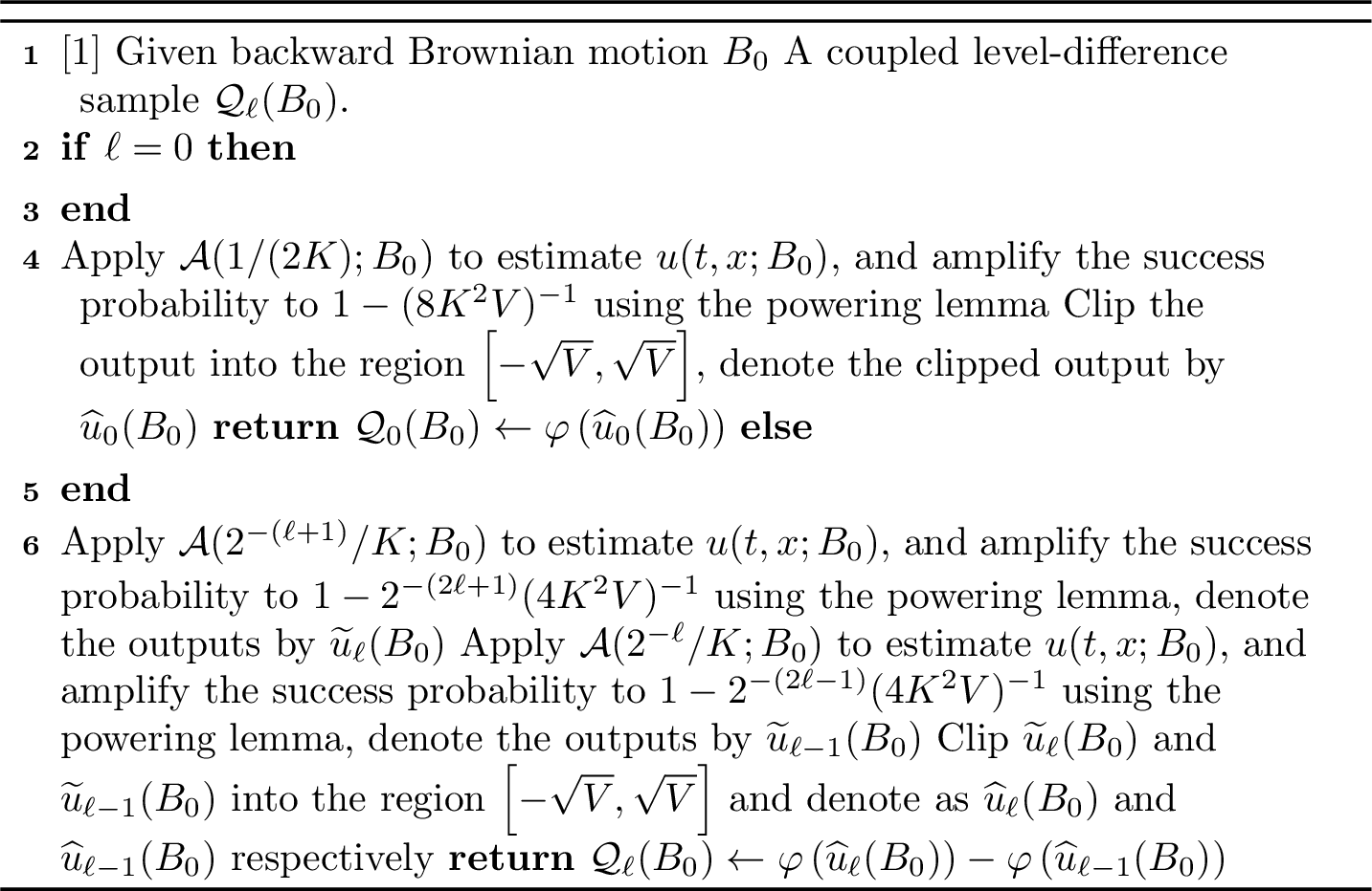
![Figure 4: Nested Quantum-accelerated MLMC Estimator for \theta=\mathbb{E}_{B}\left[\varphi(u(t,x;B))\right]](/article/2606.31076/_pdflatex/qzkisjme.png "fig:")
Theorem 4. Under the assumptions of Theorem 3, assume further that \(\varphi:\mathbb{R}\to\mathbb{R}\) is globally Lipschitz, namely, there exists \(K>0\) such that \(|\varphi(x)-\varphi(y)| \le K|x-y|\), \(x,y\in\mathbb{R},\) the outer variance satisfies \(\operatorname{Var}_{B}\!\left(\varphi(u(t,x;B))\right)\le S,\) and the conditional second moment of the payoff satisfies \(\mathbb{E}\!\left[|P(t,x;B_0)|^2\right]\le V\) for every realization \(B_0\) of \(B\).
Let \(\mathcal{Q}_\ell(B)\) be defined in Algorithm 3 and let \(\widehat\theta\) be the output of Algorithm 4. Then, for any \(\epsilon\in(0,1)\), \(\widehat\theta\) is a quantum estimator of \(\mathbb{E}\left[\varphi(u(t,x))\right]\)(\(=\mathbb{E}_B\left[\varphi(u(t,x;B))\right]\)) with additive error \(\epsilon\) and success probability at least 0.8, the total cost is \(\widetilde{\mathcal{O}}(\epsilon^{-1})\).
Remark 3. Recall that \(P(t,x;B)\) is defined in ?? . For a fixed realization of the backward Brownian motion \(B\), we have \(u(t,x;B)=\mathbb{E}[P(t,x;B)]\), where the expectation is taken over the stochasticity of the forward SDE.
Proof. Following the notation of Algorithm 3, we have \[\begin{align} \mathcal{Q}_\ell(B)= \begin{cases} \varphi(\widehat u_0(B)), & \ell=0,\\ \varphi(\widehat u_\ell(B))-\varphi(\widehat u_{\ell-1}(B)), & \ell\geq 1, \end{cases} \qquad \widehat u_\ell(B)\in[-\sqrt{V},\sqrt{V}]. \end{align}\]
Let \[\begin{align} m_\ell := \mathbb{E}[\mathcal{Q}_\ell(B)]. \end{align}\] By the guarantee of quantum mean estimation, with the success probability specified in Algorithm 4, we have \[\begin{align} |\widehat m_\ell-m_\ell| \leq \frac{\epsilon}{2L+2}, \qquad 0\leq \ell\leq L , \end{align}\] and \[\begin{align} \sum_{\ell=0}^L |\widehat m_\ell-m_\ell| \leq (L+1)\frac{\epsilon}{2L+2} = \frac{\epsilon}{2}. \end{align}\]
By the construction of Algorithm 3, \[\begin{align} \sum_{\ell=0}^L m_\ell = \mathbb{E}\!\left[\varphi(\widehat u_L(B))\right]. \end{align}\] Therefore, for \(\theta=\mathbb{E}_B\!\left[\varphi(u(t,x;B))\right],\) we obtain \[\begin{align} |\widehat\theta-\theta| &\leq \left| \sum_{\ell=0}^L \widehat m_\ell - \sum_{\ell=0}^L m_\ell \right| + \left| \sum_{\ell=0}^L m_\ell-\theta \right| \\ &\leq \sum_{\ell=0}^L |\widehat m_\ell-m_\ell| + \left| \mathbb{E}\!\left[\varphi(\widehat u_L(B))\right] - \mathbb{E}_B\!\left[\varphi(u(t,x;B))\right] \right| \\ &\leq \frac{\epsilon}{2} + K\mathbb{E}\!\left[ |\widehat u_L(B)-u(t,x;B)| \right]. \end{align}\]
Next, we bound the second term. By the construction in Algorithm 3, for \(\ell\geq 0\), the estimator \(\widetilde{u}_\ell(B_0)\) satisfies \[\begin{align} \left|\widetilde{u}_\ell(B_0)-u(t,x;B_0)\right| \leq \frac{2^{-(\ell+1)}}{K} \end{align}\] with failure probability at most \[\begin{align} p_\ell = 2^{-(2\ell+1)}(4K^2V)^{-1}. \end{align}\] Since \[\begin{align} |u(t,x;B_0)| = \left|\mathbb{E}_W[P(t,x;B_0)]\right| \leq \left(\mathbb{E}_W[|P(t,x;B_0)|^2]\right)^{1/2} \leq \sqrt V, \end{align}\] and since the clipping map onto \([-\sqrt V,\sqrt V]\) is nonexpansive, we have on the success event \[\begin{align} |\widehat u_\ell(B_0)-u(t,x;B_0)| \leq |\widetilde{u}_\ell(B_0)-u(t,x;B_0)| \leq \frac{2^{-(\ell+1)}}{K}. \end{align}\] On the failure event, both \(\widehat u_\ell(B_0)\) and \(u(t,x;B_0)\) belong to \([-\sqrt V,\sqrt V]\), and hence \[\begin{align} |\widehat u_\ell(B_0)-u(t,x;B_0)| \leq 2\sqrt V. \end{align}\] Consequently, \[\begin{align} \mathbb{E}\!\left[ |\widehat u_\ell(B)-u(t,x;B)|^2 \right] &\leq \left(\frac{2^{-(\ell+1)}}{K}\right)^2 +(2\sqrt V)^2 \cdot 2^{-(2\ell+1)}(4K^2V)^{-1} \\ &\leq K^{-2}2^{-2\ell}. \end{align}\] Therefore, \[\begin{align} K\mathbb{E}\!\left[ |\widehat u_L(B)-u(t,x;B)| \right] &\leq K \left( \mathbb{E}\!\left[ |\widehat u_L(B)-u(t,x;B)|^2 \right] \right)^{1/2} \\ &\leq 2^{-L} \leq \frac{\epsilon}{2}, \end{align}\] where the last inequality follows from \(L=\lceil \log_2(2/\epsilon)\rceil\). Thus, on the joint success event, \[\begin{align} |\widehat\theta-\theta|\leq \epsilon . \end{align}\]
For the success probability, the failure probability of the level-\(0\) outer mean estimation is at most \(0.1\), and the failure probabilities of the remaining outer mean estimations are bounded by \(\sum_{\ell=1}^{\infty}0.01^\ell<0.02\). Hence the overall success probability is at least \[\begin{align} 1-0.1-\sum_{\ell=1}^{\infty}0.01^\ell >0.8 . \end{align}\]
Next, we consider the computational complexity of Algorithm 4. By the construction in Algorithm 3, we have \[\begin{align} \left|\widetilde{u}_\ell(B_0)-u(t,x;B_0)\right|\leq 2^{-(\ell+1)}/K \end{align}\] with probability at least \(1-2^{-(2\ell+1)}(4K^2V)^{-1}\). Since \(\mathbb{E}\left[|P(t,x;B_0)|^2 \right]\leq V\), we known \[|u(t,x;B_0)|=\left|\mathbb{E}\left[P(t,x;B_0) \right]\right|\leq \sqrt{V}.\]
So \[\begin{align} \mathbb{E}\left[\left|\widehat u_{\ell}(B)-u(t,x;B)\right|^2\right] \leq \left(2^{-(\ell+1)}/K\right)^2+(2\sqrt{V})^2\cdot 2^{-(2\ell+1)}(4K^2V)^{-1}\leq K^{-2}2^{-2\ell}. \end{align}\]
For \(\ell\geq 1\), since \(\varphi\) is globally \(K\)-Lipschitz, we have \[\begin{align} \operatorname{Var}\left(\mathcal{Q}_\ell(B)\right) &\leq \mathbb{E}\left[\mathcal{Q}_\ell(B)^2\right]\\ &= \mathbb{E}\left[\left|\varphi(\widehat u_\ell(B))-\varphi(\widehat u_{\ell-1}(B))\right|^2\right] \\ &\leq 2\mathbb{E}\left[\left|\varphi(\widehat u_\ell(B))-\varphi( u(t,x;B))\right|^2\right] +2\mathbb{E}\left[\left|\varphi(\widehat u_{\ell-1}(B))-\varphi( u(t,x;B))\right|^2\right]\\ &\leq 2K^2\mathbb{E}\left[\left|\widehat u_\ell(B)- u(t,x;B)\right|^2\right] +2K^2\mathbb{E}\left[\left|\widehat u_{\ell-1}(B)- u(t,x;B)\right|^2\right]\\ &\leq 16\cdot2^{-2\ell} . \end{align}\]
By Theorem 3, Lemma 1 and powering lemma, for \(\ell\geq 1\), the cost of estimating \(\mathbb{E}_B[\mathcal{Q}_\ell(B)]\) is \[\begin{align} \mathcal{O}((2L+2)/\epsilon\times 2^{-\ell}\times \log(100^\ell))\times \widetilde{\mathcal{O}} \left(2^{\ell+1}K\times \log(2^{-(2\ell+1)}(4K^2V)^{-1})\right) =\widetilde{\mathcal{O}} \left(KLl^2/\epsilon\right). \end{align}\] Here, the first term corresponds to the number of queries required to estimate \(\mathbb{E}_B[\mathcal{Q}_\ell(B)]\), while the second term represents the computational cost of a single query to \(\mathcal{Q}_\ell(B)\), as given by Theorem 3.
For \(\ell=0\), the variance is bounded by \(2S+1\) under our assumptions, and hence the computational complexity is \(\mathcal{O}(SL/\epsilon)\).
Summing up all the \(L\) costs together yields a total cost of \(\widetilde{\mathcal{O}}(\epsilon^{-1})\). ◻
Remark 4. Note that the conditional expectation framework of Section 3.1 and the nested expectation framework of Section 3.2 depend only on the existence of a representation of the form \[\begin{align} Q(t,x;B) = \mathbb{E}_W[\mathcal{P}(t,x;B)\mid B], \end{align}\] where \(\Pi\) is a stochastic path functional.
The specific structure of the underlying SPDE enters the framework only through the choice of \(\Pi\). Consequently, the conditional and nested QA-MLMC methodologies developed above apply without modification to any quantity admitting a representation of this form.
In the subsequent sections, we will construct such path functionals \(\mathcal{P}\) for the SPDE solution itself and for the associated first- and second-order Greek estimators.
4 Applications to Derivative Pricing and Sensitivity Analysis↩︎
This section specializes the conditional and nested QA-MLMC framework of Sections 2–3 to derivative pricing and sensitivity analysis. The common structure is the following: after fixing the backward Brownian path \(B\), each target quantity is represented as \[\mathbb{E}_W[\mathcal{P}(t,x;B)\mid B],\] where \(\mathcal{P}(t,x;B)\) is a scalar path functional of the forward diffusion. Once such a representation is available, the same dyadic fine–coarse coupling and the same quantum mean estimation routine used for the price can be applied to the corresponding payoff register.
Throughout this section, unless otherwise stated, we work in the scalar case \(k=1\). Vector-valued claims are obtained componentwise. We write \(\mathbb{E}_W[\cdot\mid B]\) for expectation over the forward Brownian motion after conditioning on the realization of the backward Brownian motion \(B\). The terminal function in the BDSDE representation is denoted by \(G\); when the terminal condition is written as \(g\) elsewhere in the paper, one simply sets \(G=g\).
4.1 Conditional Pricing under Common Noise↩︎
By ?? –?? , the conditional value of the linear backward SPDE is \[\label{eq:app-price-representation} u(t,x;B) = \mathbb{E}_W\!\left[P(t,x;B)\mid B\right],\tag{8}\] where \[\begin{align} \label{eq:app-payoff-functional} P(t,x;B) &= \Phi(t,T)\,G\!\left(X_T^{t,x}\right) +\int_t^T \Phi(t,s) \Big(F(s,X_s^{t,x})+d(s)H(s,X_s^{t,x})\Big)\,\mathrm ds +\int_t^T \Phi(t,s)H(s,X_s^{t,x})\,\mathrm d \overleftarrow{B}_s. \end{align}\tag{9}\] Here \(X^{t,x}\) is the forward diffusion driven by \(W\), while the backward stochastic integral is evaluated along the fixed path \(B\).
4.1.0.1 Pure discounted pricing.
For a European claim with discounted terminal payoff only, take \[\label{eq:app-pure-pricing} G(x)=g(x),\quad F\equiv0,\quad H\equiv0,\quad c(s)=-r(s),\quad d(s)=\widetilde{c}(s)=0 .\tag{10}\] Then \[\label{eq:app-european-price} u(t,x;B) = \mathbb{E}_W\!\left[ \exp\!\left(-\int_t^T r(s)\,\mathrm ds\right) g\!\left(X_T^{t,x}\right) \;\middle|\; B \right].\tag{11}\] In this pure terminal-payoff case, the dependence on \(B\) disappears unless the forward model itself contains common-noise coefficients. Nonzero \(F\) covers running cashflows, and nonzero \(H\) encodes exposure to the backward common-noise factor.
4.1.0.2 Compatibility with the QA-MLMC algorithms.
For each level \(\ell\), let \(P_\ell(t,x;B)\) be the time-discretized version of 9 generated by the operators \[(\mathcal{S}_X,\mathcal{S}_\Phi,\mathcal{S}_{\mathrm{int}})\] and by the same dyadic Brownian coupling as in Algorithm 1. The conditional telescoping identity is \[\label{eq:app-price-telescoping} \mathbb{E}_W[P_L(t,x;B)\mid B] = \mathbb{E}_W[P_0(t,x;B)\mid B] + \sum_{\ell=1}^L \mathbb{E}_W[P_\ell(t,x;B)-P_{\ell-1}(t,x;B)\mid B].\tag{12}\] Therefore Algorithm 2 estimates \(u(t,x;B)\). The unconditional price \[\label{eq:app-unconditional-price} U(t,x):=\mathbb{E}_B[u(t,x;B)]\tag{13}\] is obtained by Algorithm 4 with \(\varphi(z)=z\).
4.2 First-order Greeks for Smooth Payoffs↩︎
We first treat pathwise first-order Greeks. In this subsection the coefficients \(c,\widetilde{c},d\) are deterministic functions of time, as in the linear BDSDE representation. Hence the exponential weight \(\Phi(t,s)\) depends on \(W\) and \(B\), but not on the initial state \(x\). If one allows state-dependent discounting or state-dependent coefficients in \(\Phi\), then the corresponding spatial derivatives of \(\Phi\) must be added to the formulas below.
Proposition 1 (Pathwise representation of conditional first-order Greeks). Let the forward Brownian motion have dimension \(d\), and let \(\sigma_{\cdot a}\) denote the \(a\)th column of \(\sigma\). Assume that \(b,\sigma\in C_b^2\) in the spatial variable, that \(G\in C_p^2(\mathbb{R}^d)\), and that \(F,H\in C_b^2([0,T]\times\mathbb{R}^d)\). Assume also the usual moment bounds that justify differentiation under \(\mathbb{E}_W[\cdot\mid B]\).
Define the Jacobian flow \[\label{eq:app-jacobian} J_s^{t,x}:=\nabla_x X_s^{t,x}\in\mathbb{R}^{d\times d}, \quad J_t^{t,x}=I_d .\qquad{(6)}\] Then \(J^{t,x}\) solves \[\label{eq:app-jacobian-sde} dJ_s^{t,x} = \nabla_x b(X_s^{t,x})J_s^{t,x}\,ds + \sum_{a=1}^{d} \nabla_x\sigma_{\cdot a}(X_s^{t,x})J_s^{t,x}\,dW_s^a .\qquad{(7)}\] For each coordinate direction \(e_i\), define \[\label{eq:app-first-order-greek} \mathcal{G}_i(t,x;B):=\partial_{x_i}u(t,x;B).\qquad{(8)}\] Then \[\label{eq:app-first-order-greek-expectation} \mathcal{G}_i(t,x;B) = \mathbb{E}_W\!\left[P^{(i)}(t,x;B)\mid B\right],\qquad{(9)}\] where \[\begin{align} \label{eq:app-first-order-greek-payoff} P^{(i)}(t,x;B) &= \Phi(t,T)\, \nabla G(X_T^{t,x})^\top J_T^{t,x}e_i \nonumber\\ &\quad +\int_t^T \Phi(t,s)\, \nabla_x\!\Big(F(s,X_s^{t,x})+d(s)H(s,X_s^{t,x})\Big)^\top J_s^{t,x}e_i\,\mathrm ds \nonumber\\ &\quad +\int_t^T \Phi(t,s)\, \nabla_x H(s,X_s^{t,x})^\top J_s^{t,x}e_i\, \mathrm d \overleftarrow{B}_s. \end{align}\qquad{(10)}\]
Proof. Under the stated assumptions, the stochastic flow \(x\mapsto X_s^{t,x}\) is differentiable and its Jacobian solves ?? . Since \(\Phi\) is independent of the initial state \(x\) in the present linear setting, differentiating 9 pathwise gives ?? . The assumed moment bounds justify interchanging differentiation and conditional expectation, which proves ?? . ◻
4.2.1 Delta↩︎
Assume that the first state component is the spot, so that \(x=(S,\chi)\), where \(\chi\) denotes all remaining factors. The conditional Delta is \[\label{eq:app-delta} \Delta(t,x;B) := \partial_S u(t,x;B) = \mathbb{E}_W\!\left[P^{(S)}(t,x;B)\mid B\right].\tag{14}\] In the pure pricing case 10 , if \(G(x)=g(S)\) depends only on the terminal spot, then \[\label{eq:app-delta-pure} P^{(S)}(t,x;B) = \Phi(t,T)\, g'(S_T^{t,x})\,\partial_S S_T^{t,x}.\tag{15}\] Thus Delta is obtained by propagating only the tangent direction \(J_s^{t,x}e_S\).
4.2.2 Spot Vega↩︎
If the state contains an instantaneous variance or volatility factor \(V\), the spot Vega is the sensitivity with respect to that state variable: \[\label{eq:app-spot-vega} \mathcal{V}_{\mathrm{spot}}(t,x;B) := \partial_V u(t,x;B) = \mathbb{E}_W\!\left[P^{(V)}(t,x;B)\mid B\right].\tag{16}\] If \(G(x)=g(S)\) depends only on the terminal spot, then \[\label{eq:app-spot-vega-pure} P^{(V)}(t,x;B) = \Phi(t,T)\, g'(S_T^{t,x})\,\partial_V S_T^{t,x}.\tag{17}\] The dependence on the initial variance or volatility is transmitted through the tangent flow.
4.2.3 Rho and general parameter Greeks↩︎
State sensitivities are only one class of Greeks. Let \(\vartheta\) be a scalar parameter entering the forward coefficients, the terminal payoff, the running terms, or the exponential weight. We write \[X^{\vartheta,t,x},\quad \Phi^\vartheta,\quad P^\vartheta(t,x;B),\quad u^\vartheta(t,x;B) = \mathbb{E}_W[P^\vartheta(t,x;B)\mid B].\] Assume differentiability in \(\vartheta\) and sufficient moment bounds for differentiation under \(\mathbb{E}_W[\cdot\mid B]\).
Define the parameter tangent process \[\label{eq:app-parameter-tangent} U_s^\vartheta := \partial_\vartheta X_s^{\vartheta,t,x}, \quad U_t^\vartheta=0 .\tag{18}\] It solves \[\begin{align} \label{eq:app-parameter-tangent-sde} dU_s^\vartheta &= \Big[ \partial_\vartheta b^\vartheta(X_s^{\vartheta,t,x}) + \nabla_x b^\vartheta(X_s^{\vartheta,t,x})U_s^\vartheta \Big]\,ds + \sum_{a=1}^{d} \Big[ \partial_\vartheta\sigma_{\cdot a}^\vartheta(X_s^{\vartheta,t,x}) + \nabla_x\sigma_{\cdot a}^\vartheta(X_s^{\vartheta,t,x})U_s^\vartheta \Big]\,dW_s^a . \end{align}\tag{19}\]
When the coefficients \(c^\vartheta,d^\vartheta,\widetilde{c}^\vartheta\) in \(\Phi^\vartheta\) depend on \(\vartheta\), define \[\begin{align} \label{eq:app-logPhi-derivative} \Lambda_\vartheta(t,s) &:= \int_t^s \partial_\vartheta c^\vartheta(r)\,\mathrm dr + \int_t^s \partial_\vartheta d^\vartheta(r)\, \mathrm d \overleftarrow{B}_r + \int_t^s \partial_\vartheta\widetilde{c}^\vartheta(r)\,\mathrm dW_r - \int_t^s \Big( \widetilde{c}^\vartheta(r)\partial_\vartheta\widetilde{c}^\vartheta(r) - d^\vartheta(r)\partial_\vartheta d^\vartheta(r) \Big)\,\mathrm dr . \end{align}\tag{20}\] Then \[\label{eq:app-Phi-derivative} \partial_\vartheta\Phi^\vartheta(t,s) = \Phi^\vartheta(t,s)\Lambda_\vartheta(t,s).\tag{21}\] For notational compactness, write \[A^\vartheta(s,x) := F^\vartheta(s,x)+d^\vartheta(s)H^\vartheta(s,x).\] Then \[\label{eq:app-general-parameter-greek} \partial_\vartheta u^\vartheta(t,x;B) = \mathbb{E}_W\!\left[Q^{(\vartheta)}(t,x;B)\mid B\right],\tag{22}\] where \[\begin{align} \label{eq:app-general-parameter-greek-payoff} Q^{(\vartheta)}(t,x;B) &= \partial_\vartheta\Phi^\vartheta(t,T)\, G^\vartheta(X_T^{\vartheta,t,x}) + \Phi^\vartheta(t,T) \Big( \partial_\vartheta G^\vartheta(X_T^{\vartheta,t,x}) + \nabla_x G^\vartheta(X_T^{\vartheta,t,x})^\top U_T^\vartheta \Big) \nonumber\\ &\quad + \int_t^T \Big[ \partial_\vartheta\Phi^\vartheta(t,s)\, A^\vartheta(s,X_s^{\vartheta,t,x}) + \Phi^\vartheta(t,s) \Big( \partial_\vartheta A^\vartheta(s,X_s^{\vartheta,t,x}) + \nabla_x A^\vartheta(s,X_s^{\vartheta,t,x})^\top U_s^\vartheta \Big) \Big]\,\mathrm ds\notag\\ &\quad+ \int_t^T \Big[ \partial_\vartheta\Phi^\vartheta(t,s)\, H^\vartheta(s,X_s^{\vartheta,t,x}) + \Phi^\vartheta(t,s) \Big( \partial_\vartheta H^\vartheta(s,X_s^{\vartheta,t,x}) + \nabla_x H^\vartheta(s,X_s^{\vartheta,t,x})^\top U_s^\vartheta \Big) \Big]\, \mathrm d \overleftarrow{B}_s. \end{align}\tag{23}\]
4.2.3.1 Discount-only Rho.
If the short rate enters only through the discount coefficient \(c^\eta(s)=-r^\eta(s)\), with \[r^\eta(s)=r(s)+\eta\psi(s),\] and all other coefficients, including the forward dynamics, are kept fixed, then in the pure pricing setting 10 , \[\label{eq:app-rho-discount-only} \mathrm{Rho}^{\mathrm{disc}}_{\psi}(t,x;B) := \left.\partial_\eta u^\eta(t,x;B)\right|_{\eta=0} = - \mathbb{E}_W\!\left[ \left(\int_t^T\psi(s)\,\mathrm ds\right) \Phi(t,T)G(X_T^{t,x}) \;\middle|\;B \right].\tag{24}\] For a constant short-rate shift, \(\psi\equiv1\), \[\label{eq:app-rho-discount-only-constant} \mathrm{Rho}^{\mathrm{disc}}(t,x;B) = -(T-t)u(t,x;B).\tag{25}\] This identity is a discount-only identity. In risk-neutral equity models where \(r\) also enters the drift of \(X\), the full Rho must instead be computed from 23 , including the parameter tangent \(U^\vartheta\).
4.2.3.2 Discrete parameter Greeks.
For the augmented Milstein dynamics of Section 5, let \[\widetilde{X}_n=(S_n,V_n,D_n,Y_n,Z_n)\] and write one step as \[\widetilde{X}_{n+1} = \mathcal{S}(\widetilde{X}_n;\xi_n),\] where \(\xi_n\) collects the Brownian increments and any iterated stochastic integrals required by the scheme. A discrete parameter Greek is obtained by propagating \[\label{eq:app-discrete-parameter-tangent} \dot{\widetilde{X}}_{n+1} = \nabla_{\widetilde{X}}\mathcal{S}(\widetilde{X}_n;\xi_n) \dot{\widetilde{X}}_n + \partial_\vartheta\mathcal{S}(\widetilde{X}_n;\xi_n).\tag{26}\] The terminal Greek payoff is obtained by differentiating the terminal payoff register, for example \[D_NG(S_N)+Y_N+Z_N .\] This covers full Rho as well as model-parameter sensitivities such as \(\partial_\kappa u\), \(\partial_\xi u\), \(\partial_\rho u\), and \(\partial_\theta u\).
4.3 Second-order Greeks for Smooth Payoffs↩︎
Second-order Greeks are obtained by differentiating the pathwise first-order representation once more.
Proposition 2 (Pathwise representation of conditional second-order Greeks). Assume that \(b,\sigma\in C_b^3\) in the spatial variable, that \(G\in C_p^3(\mathbb{R}^d)\), and that \(F,H\in C_b^3([0,T]\times\mathbb{R}^d)\). Assume the corresponding moment bounds needed for differentiating under \(\mathbb{E}_W[\cdot\mid B]\).
For \(i,j\in\{1,\ldots,d\}\), define \[\label{eq:app-second-tangent} K_s^{(ij),t,x} := \partial_{x_i x_j}^2X_s^{t,x}, \quad K_t^{(ij),t,x}=0 .\qquad{(11)}\] Let \(J_s^i:=J_s^{t,x}e_i\). Then \[\begin{align} \label{eq:app-second-tangent-sde} dK_s^{(ij),t,x} &= \Big[ \nabla_x b(X_s^{t,x})K_s^{(ij),t,x} + \nabla_x^2 b(X_s^{t,x})[J_s^i,J_s^j] \Big]\,ds + \sum_{a=1}^{d} \Big[ \nabla_x\sigma_{\cdot a}(X_s^{t,x})K_s^{(ij),t,x} +\nabla_x^2\sigma_{\cdot a}(X_s^{t,x})[J_s^i,J_s^j] \Big]\,dW_s^a . \end{align}\qquad{(12)}\] Moreover, \[\label{eq:app-second-order-greek} \mathcal{G}_{ij}^{(2)}(t,x;B) := \partial_{x_i x_j}^2u(t,x;B) = \mathbb{E}_W\!\left[P^{(ij)}(t,x;B)\mid B\right],\qquad{(13)}\] where \[\begin{align} \label{eq:app-second-order-greek-payoff} P^{(ij)}(t,x;B) &= \Phi(t,T) \Big( (J_T^j)^\top\nabla_x^2G(X_T^{t,x})J_T^i + \nabla_xG(X_T^{t,x})^\top K_T^{(ij),t,x} \Big) \nonumber\\ &\quad + \int_t^T \Phi(t,s) \Big( (J_s^j)^\top \nabla_x^2\!\big(F+dH\big)(s,X_s^{t,x})J_s^i + \nabla_x\!\big(F+dH\big)(s,X_s^{t,x})^\top K_s^{(ij),t,x} \Big)\,\mathrm ds \nonumber\\ &\quad + \int_t^T \Phi(t,s) \Big( (J_s^j)^\top\nabla_x^2H(s,X_s^{t,x})J_s^i + \nabla_xH(s,X_s^{t,x})^\top K_s^{(ij),t,x} \Big)\, \mathrm d \overleftarrow{B}_s. \end{align}\qquad{(14)}\] Here \(\nabla_x^2 a(x)[u,v]\) denotes the bilinear action of the Hessian of \(a\) on the pair \((u,v)\).
Proof. Differentiate ?? with respect to the initial coordinate \(x_j\). The \(C_b^3/C_p^3\) regularity assumptions give the second derivative of the stochastic flow and the SDE ?? . The chain rule yields ?? , and the moment assumptions justify passing the derivative through the conditional expectation. ◻
4.3.1 Gamma↩︎
When \(x=(S,\chi)\) and the first component is the spot, the conditional Gamma is \[\label{eq:app-gamma} \Gamma(t,x;B) := \partial_{SS}u(t,x;B) = \mathbb{E}_W\!\left[P^{(SS)}(t,x;B)\mid B\right].\tag{27}\] In the pure pricing case 10 , if \(G(x)=g(S)\), then \[\label{eq:app-gamma-pure} P^{(SS)}(t,x;B) = \Phi(t,T) \left[ g''(S_T^{t,x})(\partial_SS_T^{t,x})^2 + g'(S_T^{t,x})\partial_{SS}^2S_T^{t,x} \right].\tag{28}\]
4.3.2 Vanna and Volga↩︎
If the state contains a variance or volatility factor \(V\), then \[\label{eq:app-vanna-volga} \mathrm{Vanna}(t,x;B) := \partial_{SV}u(t,x;B) = \mathbb{E}_W\!\left[P^{(SV)}(t,x;B)\mid B\right], \quad \mathrm{Volga}(t,x;B) := \partial_{VV}u(t,x;B) = \mathbb{E}_W\!\left[P^{(VV)}(t,x;B)\mid B\right].\tag{29}\] If \(G(x)=g(S)\) depends only on the terminal spot, then \[\begin{align} P^{(SV)}(t,x;B) &= \Phi(t,T) \left[ g''(S_T^{t,x}) \partial_SS_T^{t,x}\, \partial_VS_T^{t,x} + g'(S_T^{t,x})\partial_{SV}^2S_T^{t,x} \right], \tag{30} \\ P^{(VV)}(t,x;B) &= \Phi(t,T) \left[ g''(S_T^{t,x}) (\partial_VS_T^{t,x})^2 + g'(S_T^{t,x})\partial_{VV}^2S_T^{t,x} \right]. \tag{31} \end{align}\]
4.4 Greek Estimators in the MLMC and QA-MLMC Pipeline↩︎
The formulas above identify the exact scalar random variables whose conditional expectations are the Greeks. To use them in the algorithms, one augments the one-step discretization by tangent variables.
4.4.0.1 First-order Greeks.
Let \[\xi_k\] collect all random inputs required by the one-step scheme, including \(\Delta W_k\), \(\Delta\overleftarrow B_k\), and, when used, mixed iterated integrals such as \(J_{t_k,h}^{WB}\). A first-order Greek discretization has the form \[\label{eq:app-discrete-jacobian} J_{k+1} = \mathcal{S}_J(J_k,X_k,t_k,h;\Delta W_{t_k},\Delta\overleftarrow B_{t_k}),\tag{32}\] together with a Greek-payoff update \[\label{eq:app-discrete-first-order-payoff} Y_{k+1}^{(i)} = Y_k^{(i)} + \mathcal{S}_{\mathrm{int}}^{(i)} \big( \Phi_k,X_k,J_k,t_k,h;\Delta W_{t_k},\Delta\overleftarrow B_{t_k} \big),\tag{33}\] whose terminal value approximates ?? .
4.4.0.2 Second-order Greeks.
For second-order sensitivities, add \[\label{eq:app-discrete-second-tangent} K_{k+1}^{(ij)} = \mathcal{S}_K\left(K_k^{(ij)},J_k,X_k,t_k,h;\Delta W_{t_k},\Delta\overleftarrow B_{t_k}\right),\tag{34}\] and \[\label{eq:app-discrete-second-order-payoff} Y_{k+1}^{(ij)} = Y_k^{(ij)} + \mathcal{S}_{\mathrm{int}}^{(ij)} \big( \Phi_k,X_k,J_k,K_k^{(ij)},t_k,h;\Delta W_{t_k},\Delta\overleftarrow B_{t_k} \big),\tag{35}\] whose terminal value approximates ?? .
Using the same dyadic Brownian coupling as in Algorithm 1, define the level differences \[\label{eq:app-greek-level-differences} \Delta_\ell^{(i)} := P_\ell^{(i,f)}-P_{\ell-1}^{(i,c)}, \quad \Delta_\ell^{(ij)} := P_\ell^{(ij,f)}-P_{\ell-1}^{(ij,c)} .\tag{36}\] These level differences are fed into Algorithm 2 in exactly the same way as the price level differences.
Corollary 1 (Conditional QA-MLMC for smooth Greeks). Assume the hypotheses of Proposition 1. Assume also that the augmented first-order discretization \[(\mathcal{S}_X,\mathcal{S}_\Phi,\mathcal{S}_J, \mathcal{S}_{\mathrm{int}}^{(i)})\] has strong-error order at least \(1\), satisfies the required accumulated stability estimate, and has uniformly bounded moments of sufficiently high order. Then \[\left| \mathbb{E}_W[P_\ell^{(i)}-P^{(i)}\mid B] \right| = \mathcal{O}(2^{-\ell}), \quad \operatorname{Var}_W(P_\ell^{(i)}-P_{\ell-1}^{(i)}\mid B) = \mathcal{O}(2^{-2\ell}), \quad C_\ell=\mathcal{O}(2^\ell).\] Consequently, Algorithm 2, with the price payoff register replaced by the first-order Greek payoff register, estimates \(\mathcal{G}_i(t,x;B)\) with additive error \(\epsilon\) and cost \(\widetilde{\mathcal{O}}(\epsilon^{-1})\).
If, in addition, the augmented second-order discretization \[(\mathcal{S}_X,\mathcal{S}_\Phi,\mathcal{S}_J,\mathcal{S}_K, \mathcal{S}_{\mathrm{int}}^{(ij)})\] has strong-error order at least \(1\), satisfies the analogous stability estimate, and has the required moment bounds, then the same conclusion holds for \(\mathcal{G}_{ij}^{(2)}(t,x;B)=\partial_{x_i x_j}^2u(t,x;B)\).
Proof. The proof is the same as the proof of Theorem 3. The Greek payoff is still a scalar path functional. For any fixed Greek, the tangent variables enlarge the state dimension only by a constant factor, so the cost exponent remains \(\gamma=1\). The assumed strong-error order gives \(\alpha=1\) and \(\beta=2\) in Theorem 2. Therefore the conditional quantum MLMC cost is \(\widetilde{\mathcal{O}}(\epsilon^{-1})\). ◻
Corollary 2 (Nested QA-MLMC for unconditional Greeks). Let \[U(t,x):=\mathbb{E}_B[u(t,x;B)].\] In addition to the assumptions of Corollary 1, assume that differentiation may be interchanged with the outer expectation over \(B\), for example by dominated convergence or by a uniform integrability condition on the conditional Greek payoffs. Assume also \[\sup_{B_0} \mathbb{E}_W\!\left[|P^{(i)}(t,x;B_0)|^2\mid B_0\right] <\infty,\] and, for second-order Greeks, \[\sup_{B_0} \mathbb{E}_W\!\left[|P^{(ij)}(t,x;B_0)|^2\mid B_0\right] <\infty .\] Then nested QA-MLMC yields estimators of \[\partial_{x_i}U(t,x) = \mathbb{E}_B[\mathcal{G}_i(t,x;B)]\] and \[\partial_{x_i x_j}^2U(t,x) = \mathbb{E}_B[\mathcal{G}_{ij}^{(2)}(t,x;B)]\] with additive error \(\epsilon\) and total cost \(\widetilde{\mathcal{O}}(\epsilon^{-1})\).
Proof. Apply Theorem 4 with \(\varphi(z)=z\), replacing the inner conditional price estimator by the corresponding conditional Greek estimator. The interchange condition identifies the outer expectation of the conditional Greek with the Greek of the unconditional value function. ◻
4.5 Nonsmooth Payoffs: Likelihood-ratio and Malliavin-weight Greeks↩︎
The pathwise Greek formulas above were stated under differentiability assumptions on the terminal function \(G\). Hence they do not directly cover nonsmooth payoffs. For Lipschitz payoffs with isolated kinks, such as vanilla calls, first-order pathwise estimators may still be justified under suitable non-atomicity or density assumptions on \(X_T^{t,x}\). However, discontinuous payoffs, barrier-type path functionals, and higher-order Greeks generally require additional smoothing, likelihood-ratio, or Malliavin integration-by-parts arguments [68]–[70].
For illustration, consider the pure terminal-value case 10 , so that \(F=H=0\), \(c=-r\), and \(d=\widetilde{c}=0\). In this case \(\Phi(t,T)\) is independent of the forward Brownian motion after conditioning on \(B\). Assume that the forward diffusion is sufficiently smooth and uniformly elliptic, with \[a(s,x):=\sigma(s,x)\sigma(s,x)^\top \succeq \lambda I_d\] for some \(\lambda>0\).
If the transition density \(p(t,x;T,y)\) exists and is differentiable with respect to the initial condition \(x\), then the likelihood-ratio representation has the form [68] \[\label{eq:app-lr-greek} \partial_{x_i}u(t,x;B) = \mathbb{E}_W\!\left[ \Phi(t,T)G(X_T^{t,x}) \,\partial_{x_i}\log p(t,x;T,X_T^{t,x}) \;\middle|\;B \right].\tag{37}\]
Alternatively, one may use a Malliavin-weight representation. Define \[\label{eq:app-bel-weight-general} \mathcal{W}_i(t,T) := \frac{1}{T-t} \int_t^T \left( \sigma(s,X_s^{t,x})^\top a(s,X_s^{t,x})^{-1} J_s^i \right)^\top \mathrm dW_s .\tag{38}\] When \(\sigma\) is square and invertible, this reduces to \[\label{eq:app-bel-weight-square} \mathcal{W}_i(t,T) = \frac{1}{T-t} \int_t^T \left( \sigma(s,X_s^{t,x})^{-1}J_s^i \right)^\top \mathrm dW_s .\tag{39}\] The Bismut–Elworthy–Li formula then gives [69], [71], [72] \[\label{eq:app-bel-directional} \partial_{x_i}u(t,x;B) = \mathbb{E}_W\!\left[ \Phi(t,T)G(X_T^{t,x})\,\mathcal{W}_i(t,T) \;\middle|\;B \right].\tag{40}\] Thus the derivative is again represented as the conditional expectation of a scalar path functional, with the payoff derivative replaced by a stochastic weight.
The simple form 40 uses the fact that, in the pure terminal-value setting, \(\Phi(t,T)\) is independent of \(W\). If \(\widetilde{c}\neq0\), or more generally if the exponential factor or running payoff contains \(W\)-dependent terms, the Malliavin integration-by-parts formula must also account for the Malliavin derivative of those terms. Such general weighted representations can still be incorporated into the same conditional-expectation framework, but the weight and payoff register must be modified accordingly.
The conditional and nested QA-MLMC architecture can be applied to these weighted-payoff estimators once the corresponding discretized weighted payoff registers satisfy the same bias, variance-decay, cost, and moment assumptions used in Corollaries 1 and 2. In particular, one needs \[\left| \mathbb{E}_W[P_{\ell}^{\mathrm{w}}-P^{\mathrm{w}}\mid B] \right| = O(2^{-\ell}), \quad \operatorname{Var}_W(P_{\ell}^{\mathrm{w}}-P_{\ell-1}^{\mathrm{w}}\mid B) = O(2^{-2\ell}), \quad C_\ell=O(2^\ell),\] together with sufficient moment or tail bounds for the likelihood-ratio or Malliavin weight. If the weight is unbounded, clipping or truncation may be used only after controlling the induced bias at the target accuracy. Barrier and other path-dependent discontinuous payoffs require path-dependent Malliavin weights or conditional-smoothing arguments and are not covered by the terminal-value formula above [69], [73], [74].
4.6 Heston-type Stochastic-volatility Models↩︎
As a canonical two-factor example, consider the Heston stochastic-volatility model [2]. To match the independent Brownian-input convention used in the algorithms, write \[\label{eq:app-heston} \begin{align} dS_s &= rS_s\,ds+\sqrt{V_s}S_s\,dW_s^{(1)},\\ dV_s &= \kappa(\theta-V_s)\,ds + \xi\sqrt{V_s} \left( \rho\,dW_s^{(1)} + \sqrt{1-\rho^2}\,dW_s^{(2)} \right), \end{align}\tag{41}\] where \(W^{(1)}\) and \(W^{(2)}\) are independent Brownian motions. Equivalently, one may use correlated Brownian motions with \(d\langle W^{(1)},W^{(2)}\rangle_s=\rho\,ds\).
With state vector \(x=(S,V)\), the conditional sensitivities above become \[\Delta=\partial_Su,\quad \mathcal{V}_{\mathrm{spot}}=\partial_Vu,\quad \Gamma=\partial_{SS}u,\quad \mathrm{Vanna}=\partial_{SV}u,\quad \mathrm{Volga}=\partial_{VV}u.\] Rho and the model-parameter Greeks \[\partial_\kappa u,\quad \partial_\theta u,\quad \partial_\xi u,\quad \partial_\rho u\] are computed using the parameter-tangent formulas 19 or, at the discrete level, 26 .
Remark 5. The map \(v\mapsto\sqrt v\) is not \(C^1\) at \(v=0\), and the full-truncation map \(v\mapsto v^+\) used in many numerical schemes is also nonsmooth [75]. Therefore, the global pathwise assumptions of Propositions 1 and 2 do not hold for the unregularized Heston diffusion without additional localization or moment arguments. A rigorous application of the smooth-Greek corollaries should therefore use one of the following routes:
replace \(\sqrt v\) by a smooth positive regularization, such as \(\sqrt{v+\delta}\) or another smooth approximation, and analyze the regularization bias;
localize the process to the region \(V_s\geq \epsilon\) and control the exit error;
use likelihood-ratio or Malliavin-weight estimators for nonsmooth payoffs or boundary-sensitive regimes;
use a discretization-specific tangent recursion, with a smooth truncation if differentiability of the numerical map is required.
Once the chosen model and discretization satisfy the bias, variance, stability, and moment assumptions stated in Corollaries 1 and 2, the same conditional and nested QA-MLMC complexity bounds apply to Delta, spot Vega, Gamma, Vanna, Volga, full Rho, and the Heston parameter Greeks.
5 Strong-Error Order One Schemes for Pricing and Greek Estimators↩︎
[34] developed a first-order scheme for BDSDEs based on a two-sided Itô–Taylor expansion. However, since the scheme relies on conditional expectations with respect to the forward Brownian motion at each time step, it integrates out the forward randomness and therefore does not directly provide the pathwise strong approximations required by our conditional-on-\(B\) MLMC framework. Inspired by the underlying Itô–Taylor expansion, we develop new discretization schemes and prove conditional strong-error order one convergence. Consequently, the resulting multilevel differences exhibit second-order variance decay, which is essential for retaining the quadratic quantum speedup in the QA-MLMC framework.
The BDSDE representations derived in the previous section provide probabilistic formulas for option prices and Greeks. To enable efficient multilevel Monte Carlo simulation, we construct strong-error order one discretization schemes for direct pricing estimators, first-order Greek estimators, and second-order Greek estimators.
The presentation of this section follows a common pattern for direct pricing estimators, first-order Greek estimators, and second-order Greek estimators.
For each estimator, we first derive a sufficient condition under which a generic discretization operator yields global strong convergence of order one. We then introduce a concrete Forward–Backward Taylor discretization operator and prove that it satisfies the required conditions. As a result, all three estimators admit globally first-order accurate approximations.
5.1 Forward–Backward Taylor Discretization Framework↩︎
A central contribution of our numerical scheme is a family of Forward–Backward Taylor discretizations for the path functionals appearing in the BDSDE representations of prices and Greeks.
The key challenge is that the backward stochastic integrals \[\begin{align} \int Q(r,X_r)\,\mathrm d \overleftarrow{B}_r, \end{align}\] where \(Q\) denotes a generic integrand and may represent different functions in the pricing and Greek representations. Since the integrand depends on the forward diffusion \(X\), which is itself driven by an independent Brownian motion \(W\), pathwise approximations compatible with the conditional-on-\(B\) MLMC framework must retain the dependence on both sources of randomness throughout the discretization.
Our approach is based on Taylor expansions of the stochastic integrands. The resulting discretizations naturally involve the mixed forward–backward iterated integrals \[\begin{align} J^{WB}_{s,h} &= \Big(J_{ij}^{WB}(s,h)\Big)_{1\le i\le \ell,\;1\le j\le d}, \quad J_{ij}^{WB}(s,h) := \int_s^{s+h}(W_r^j-W_s^j)\, \mathrm d \overleftarrow{B}_r^i, \tag{42} \\ J^{BB}_{s,h} &= \Big(J_{ij}^{BB}(s,h)\Big)_{1\le i,j\le \ell}, \quad J_{ij}^{BB}(s,h) := \int_s^{s+h} \bigl(B_{s}^j-B_r^j\bigr)\, \mathrm d \overleftarrow{B}_r^i, \tag{43} \end{align}\] together with the usual Brownian increments. These terms capture the interaction between the forward Brownian motion \(W\) and the backward Brownian motion \(B\), and play a crucial role in achieving strong-error order one.
Throughout this section, we consider a uniform partition \[t_k=t+kh,\quad k=0,\ldots,N,\] with stepsize \(h=(T-t)/N\). We denote the forward and backward Brownian increments by \[\Delta W_{t_k} = W_{t_{k+1}}-W_{t_k}, \quad \Delta\overleftarrow B_{t_k} = B_{t_k}-B_{t_{k+1}},\] respectively.
Unless stated otherwise, all \(L^q\) norms are taken with respect to the joint law of \((W,B)\): \[\|\cdot\|_{L^q} := \|\cdot\|_{L^q_{W,B}}.\] When conditioning on a fixed realization of the backward Brownian motion \(B\), we write the conditional norm as \(\|\cdot\|_{L_W^q}\).
5.2 Direct Pricing Estimator↩︎
Recall that the discretization operators \(\mathcal{S}_X\), \(\mathcal{S}_\Phi\), and \(\mathcal{S}_{\mathrm{int}}\) were introduced in 5 , 6 , and 7 , respectively. The goal of this subsection is to establish the strong approximation properties of these operators and to derive the accumulated stability estimates required for the global strong-error order one analysis.
Definition 1 (Strong-error order of \(S_X\)). The discretization operator \(S_X\) is said to have strong-error order \(p>0\) if there exists a constant \(C_X>0\) such that \[\begin{align} \left\| \sup_{0\leq k\leq N} \left|X_{t_k}^{t,x}-X_k^{(h)}\right| \right\|_{L^q} \leq C_Xh^{p}, \end{align}\] for every \(q\ge2\). There \(X_s^{t,x}\) is the unique strong solution to the SDE 52 and \(\{X_k^{(h)}\}_{k=0}^N\) is the discrete-time approximation generated by \[\begin{align} X_{k+1}^{(h)}=\mathcal{S}_X\left(X_k^{(h)},t_k,h;\Delta W_{t_k}\right), \quad X_0^{(h)}=x. \end{align}\]
Definition 2 (Strong-error order of \(S_\Phi\)). The discretization operator \(S_\Phi\) is said to have strong-error order \(p>0\) \[\begin{align} \left\| \sup_{0\leq k\leq N} \left| \Phi(t,t_k)-\Phi^{(h)}_k \right| \right\|_{L^q} \leq C_\Phi h^{p}, \end{align}\] for every \(q\ge2\). Here \(\{\Phi_k^{(h)}\}_{k=0}^N\) is the discrete-time approximation generated by \[\begin{align} \Phi_{k+1}^{(h)}= \mathcal{S}_\Phi\left( \Phi_k^{(h)},t_k,h;\Delta W_{t_k},\Delta\overleftarrow B_{t_k} \right), \quad \Phi_0^{(h)}=1. \end{align}\]
Definition 3 (Strong-error order of \(S_{\mathrm{int}}\)). The discretization operator \(S_{\mathrm{int}}\) is said to have strong-error order \(p>0\) if there exists a constant \(C_{\mathrm{int}}>0\) such that \[\begin{align} \left\| \sup_{0\leq k\leq N} \left| Y_{t_k}-\widetilde{Y}_k^{(h)} \right| \right\|_{L^q} \leq C_{\mathrm{int}} h^{p}, \end{align}\] for every \(q\ge2\). There \(\{\widetilde{Y}_k^{(h)}\}_{k=0}^N\) is the discrete-time payoff approximation generated by \[\begin{align} \widetilde{Y}_{k+1}^{(h)} = \widetilde{Y}_k^{(h)}+ \mathcal{S}_{\mathrm{int}}\left( \Phi(t,t_k), X_{t_{k}}^{t,x},t_{k},h;\Delta W_{t_k},\Delta\overleftarrow B_{t_k} \right), \quad \widetilde{Y}_0^{(h)}=0, \end{align}\] with \(X,\Phi\) evaluated exactly, and \(Y_{t_k}\) denotes the exact accumulated payoff process at time \(t_k\), i.e., \[\begin{align} Y_{t_k}=\int_t^{t_k}\Phi(t,r)\left(F(r,X_r^{t,x})+d(r) H(r,X_r^{t,x})\right)\,\mathrm{d}r +\int_t^{t_k}\Phi(t,r)H(r,X_r^{t,x})\mathrm d \overleftarrow{B}_r . \end{align}\]
Remark 6. For \(0<q<2\), the corresponding estimates follow from Jensen’s inequality whenever the \(q=2\) estimate is available.
After defining the strong-error order associated with each individual discretization step, we now turn to the study of the overall strong-error of the full discretized scheme. Before carrying out the detailed analysis, we first introduce the following accumulated stability property.
Definition 4 (Accumulated stability of \(\mathcal{S}_{\mathrm{int}}\)).
The discretization operator \(\mathcal{S}_{\mathrm{int}}\) is said to satisfy the accumulated stability estimate if there exists a constant \(L_{\mathrm{int}}>0\), independent of \(h\), such that \[\begin{align} \left\| \sup_{0\leq k\leq N} \left| \widetilde{Y}_k^{(h)}-Y_k^{(h)} \right| \right\|_{L^2} \leq L_{\mathrm{int}} \bigg( & \left\| \sup_{0\leq j\leq N} \left| \Phi(t,t_j)-\Phi_j^{(h)} \right| \right\|_{L^4}+ \left\| \sup_{0\leq j\leq N} \left| X_{t_j}^{t,x}-X_j^{(h)} \right| \right\|_{L^4} \bigg), \end{align}\] where \(\widetilde{Y}_k^{(h)}\) is defined in Definition 3.
Proposition 3. Fix \((t,x)\in[0,T]\times\mathbb{R}^d\) and a uniform grid \(\{t_k\}_{k=0}^N\) with \(h=(T-t)/N\). Let \[\begin{align} P_{t_k}=\Phi(t,t_k)G\left(X_{t_k}^{t,x}\right)+Y_{t_k}, \end{align}\] where \(Y_{t_k}\) is the exact accumulated payoff \[\begin{align} Y_{t_k}=\int_t^{t_k}\Phi(t,r)\left(F(r,X_r^{t,x})+d(r)H(r,X_r^{t,x})\right)\,\mathrm{d} r +\int_t^{t_k}\Phi(t,r)H(r,X_r^{t,x})\,\mathrm d \overleftarrow{B}_r. \end{align}\]
Let \(\left\{\left(X_k^{(h)},\Phi_k^{(h)}\right)\right\}_{k=0}^N\) be the approximations generated by the schemes \(S_X,S_\Phi\) as in Definition 1, 2 and define \[\begin{align} Y_{k+1}^{(h)} =& Y_k^{(h)} + \mathcal{S}_{\mathrm{int}} \left( \Phi_k^{(h)}, X_k^{(h)},t_k,h; \Delta W_{t_k}, \Delta\overleftarrow B_{t_k} \right), \quad Y_0^{(h)}=0,\\ P_k^{(h)}=&\Phi^{(h)}_k G\left(X_k^{(h)}\right)+Y_k^{(h)}. \end{align}\]
Assume:
The strong-error orders of \(\mathcal{S}_X\), \(\mathcal{S}_\Phi\) and \(\mathcal{S}_{\mathrm{int}}\) are \(p_X,p_\Phi,p_{\mathrm{int}}\) respectively. Moreover, \(\mathcal{S}_{\mathrm{int}}\) satisfies the accumulated stability estimate defined in Definition 4.
There exists \(M>0\), independent of \(h\), such that \(\Phi_k^{(h)}\) and \(G(X_{t_k}^{t,x})\) are uniformly bounded in \(L^{4}_{W,B}\) by \(M\).
\(G\) is globally Lipschitz, i.e., there exists \(L_G>0\) such that \(|G(x)-G(y)|\leq L_G|x-y|\).
Then the payoff approximation satisfies the joint strong-error bound \[\begin{align} \left\| \sup_{0\leq k\leq N} \left| P_{t_k}-P^{(h)}_k \right| \right\|_{L^2} = \mathcal{O}(h^p), \quad p=\min\{p_X,p_\Phi,p_{\mathrm{int}}\}. \end{align}\]
A detailed proof is provided in Appendix 9, Paragraph 9.1.0.1. Consequently, on a dyadic grid with \(h_\ell=2^{-\ell}\) and \(N_\ell=(T-t)2^\ell\), Lemma 2 implies the corresponding fixed-\(B\) conditional \(L_W^2\) strong-error estimate, up to the logarithmic factor \((1+\ell)^{a/2}\) for any \(a>1\).
For the forward diffusion process \(X\), we employ the Milstein discretization operator \[\begin{align} \mathcal{S}_X^{\mathrm{mil}} (x,s,h;\Delta W_s) = x +b(x)h +\sigma(x)\Delta W_s + \sum_{i=1}^{d}\sum_{j=1}^{d} L_i\sigma_j(x) \int_s^{s+h} (W_r^i-W_s^i)\,d\mathrm W_r^j, \label{eq:SX-Mil} \end{align}\tag{44}\] where \(L_i = \sum_{n=1}^{d} \sigma_{ni}(x)\partial_{x_n}.\)
For the scalar weight process \(\Phi\), we use the exponential-type discretization \[\begin{align} \mathcal{S}_\Phi (\Phi,s,h; \Delta W_s, \Delta\overleftarrow B_s) = \Phi \exp\!\Big( C_{s,h} +\widetilde{c}(s+\tfrac h2)\cdot\Delta W_s +d(s+\tfrac h2)\cdot\Delta\overleftarrow B_s -\tfrac12 Q_{s,h} \Big), \label{eq:Sphi} \end{align}\tag{45}\] where \[C_{s,h} = \frac{h}{6} \bigl( c(s)+4c(s+\tfrac h2)+c(s+h) \bigr),\] and \[Q_{s,h} = \frac{h}{6} \bigl( q(s)+4q(s+\tfrac h2)+q(s+h) \bigr), \quad q(r)=\|\widetilde{c}(r)\|^2-\|d(r)\|^2.\]
These discretizations are standard and achieve strong-error order one for the corresponding stochastic differential equations. The main additional difficulty in the present setting arises from the accumulated payoff term \[Y_{t_k} = \int_t^{t_k} \Phi(t,r) \bigl( F(r,X_r^{t,x}) + d(r)H(r,X_r^{t,x}) \bigr)\,\mathrm dr + \int_t^{t_k} \Phi(t,r)H(r,X_r^{t,x}) \mathrm d \overleftarrow{B}_r,\] whose discretization involves a backward stochastic integral. A naive Euler-type approximation yields only global strong-error order \(1/2\) and is therefore insufficient for the multilevel framework developed in this work. To overcome this difficulty, we introduce a Forward–Backward Taylor discretization operator \(\mathcal{S}_{\mathrm{int}}^{\mathrm{FBT}}\), which incorporates suitable higher-order corrections for the backward stochastic integral.
Consider the integral discretization operator \(\mathcal{S}_{\mathrm{int}}^{\mathrm{FBT}}\) defined by \[\begin{align} \mathcal{S}_{\mathrm{int}}^{\mathrm{FBT}} (\Phi,X,s,h;\Delta W_s,\Delta \overleftarrow B_s) =&\, \Phi h\bigl(F(s,X)+d(s) H(s,X)\bigr) +\Phi H(s,X)\cdot \Delta\overleftarrow B_s \notag\\ &+\Phi \sum_{i=1}^{\ell}\sum_{j=1}^{d} \bigl(H_x(s,X)\sigma(X)+\widetilde{c}(s)H(s,X)\bigr)_{ij} J_{ij}^{WB}(s,h) +\Phi \sum_{i=1}^{\ell}\sum_{j=1}^{\ell} d_j(s)H_i(s,X) J_{ij}^{BB}(s,h), \label{eq:Sint-FBT} \end{align}\tag{46}\] where \(J^{WB}_{s,h}\) and \(J^{BB}_{s,h}\) are defined in (42 )–(43 ).
Note that the first two terms in 46 coincide with the direct discretization approximation, while two additional terms \(J_{ij}^{WB}(s,h)\) and \(J_{ij}^{BB}(s,h)\) appears. These extra terms serve as higher-order corrections to the backward stochastic integral \[\int_s^{s+h}\Phi(t,r)H(r,X_r)\cdot \mathrm d \overleftarrow{B}_r,\] and are obtained from the taylor expansion of the integrand.
The following two properties explain why the integral discretization operator is defined in this way. Detailed proofs are provided in Appendix 9, Paragraphs 9.1.0.2 and 9.1.0.3.
Proposition 4 (Strong-error order of the integral discretization). Assume that \(F,H,d,\widetilde{c}\) and the coefficients of \(X\) and \(\Phi\) are sufficiently smooth with polynomial growth, and that the corresponding moments of \(X\) and \(\Phi\) are uniformly bounded. Then the approximation generated by \[\begin{align} \widetilde{Y}_{k+1}^{(h)} = \widetilde{Y}_k^{(h)} + \mathcal{S}_{\mathrm{int}}^{\mathrm{FBT}} \left(\Phi(t,t_k),X_{t_k}^{t,x}, t_k,h;\Delta W_{t_k},\Delta\overleftarrow B_{t_k}\right), \quad \widetilde{Y}_0^{(h)}=0, \end{align}\] satisfies \[\begin{align} \left\| \sup_{0\le k\le N} \left| Y_{t_k}-\widetilde{Y}_k^{(h)} \right| \right\|_{L^q} \le Ch, \end{align}\] for every \(q\ge2\). Consequently, by Jensen’s inequality, the same estimate also holds for every \(0<q<2\). Hence \(\mathcal{S}_{\mathrm{int}}^{\mathrm{FBT}}\) has strong-error order \(1\) in the sense of Definition 3.
Proposition 5. Assume that \(F,H\) are globally Lipschitz and have at most linear growth. Moreover, assume that the coefficient \(H_x(t,x)\sigma(x)+\widetilde{c}(t)H(t,x)\) is globally Lipschitz and has at most linear growth. Assume further that the exact and numerical input processes satisfy the uniform moment bound \[\left\| \sup_{0\le j\le N} |\Phi(t,t_j)| \right\|_{L^8} + \left\| \sup_{0\le j\le N} |\Phi_j^{(h)}| \right\|_{L^8} + \left\| \sup_{0\le j\le N} |X_{t_j}^{t,x}| \right\|_{L^8} + \left\| \sup_{0\le j\le N} |X_j^{(h)}| \right\|_{L^8} <\infty .\] Then \(\mathcal{S}_{\mathrm{int}}^{\mathrm{FBT}}\) satisfies the accumulated stability condition in Definition 4. More precisely, there exists \(L_{\mathrm{int}}>0\), independent of \(h\), such that \[\begin{align} \left\| \sup_{0\leq k\leq N} \left| \widetilde{Y}_k^{(h)}-Y_k^{(h)} \right| \right\|_{L^2} \le L_{\mathrm{int}} \bigg( & \left\| \sup_{0\leq j\leq N} \left| \Phi(t,t_j)-\Phi_j^{(h)} \right| \right\|_{L^4} + \left\| \sup_{0\leq j\leq N} \left| X_{t_j}^{t,x}-X_j^{(h)} \right| \right\|_{L^4} \bigg). \end{align}\]
5.3 First-Order Greek Estimators↩︎
The first-order Greek representation involves, in addition to the forward diffusion \(X\) and the weight process \(\Phi\), the Jacobian flow \(J^{t,x}\) associated with the forward SDE and a corresponding accumulated payoff term.
The purpose of this subsection is twofold. We first develop a general strong-error framework showing that the convergence rate of the first-order Greek estimator is determined by the approximation properties of the discretization operators for \(J^{t,x}\) and the accumulated payoff term. We then construct suitable discretization operators satisfying the requirements of the framework, leading to a global strong-error order one approximation for the first-order Greek estimator.
Definition 5 (Strong-error order of \(S_J\)). The discretization operator \(S_J\) is said to have strong-error order \(p>0\) if there exists a constant \(C_J>0\) such that \[\left\| \sup_{0\le k\le N} \left| J_{t_k}^{t,x}-J_k^{(h)} \right| \right\|_{L^q} \le C_J h^p\] for every \(q\ge2\). Here \(J^{t,x}\) is the Jacobian flow defined in ?? –?? , and \(\{J_k^{(h)}\}_{k=0}^N\) is generated by \[J_{k+1}^{(h)}=\mathcal{S}_J \left(J_k^{(h)},X_k^{(h)},t_k,h;\Delta W_{t_k},\Delta\overleftarrow B_{t_k}\right), \quad J_0^{(h)}=I_d .\]
Definition 6 (Strong-error order of \(S_{\mathrm{int}}^{(i)}\)). Fix \(1\le i\le d\). The discretization operator \(S_{\mathrm{int}}^{(i)}\) is said to have strong-error order \(p>0\) if there exists a constant \(C_{\mathrm{int}}^{(i)}>0\) such that \[\left\| \sup_{0\le k\le N} \left| Y_{t_k}^{(i)}-\widetilde{Y}_k^{(i,h)} \right| \right\|_{L^q} \le C_{\mathrm{int}}^{(i)} h^p\] for every \(q\ge2\). Here \[Y_{t_k}^{(i)}=\int_t^{t_k}\Phi(t,s) \nabla_x\!\Big(F(s,X_s^{t,x})+d(s)H(s,X_s^{t,x})\Big)^\top J_s^{t,x}e_i\,\mathrm ds+ \int_t^{t_k}\Phi(t,s)\nabla_xH(s,X_s^{t,x})^\top J_s^{t,x}e_i\,\mathrm d \overleftarrow{B}_s.\] The approximation \(\{\widetilde{Y}_k^{(i,h)}\}_{k=0}^N\) is generated by \[\widetilde{Y}_{k+1}^{(i,h)} =\widetilde{Y}_k^{(i,h)} +\mathcal{S}_{\mathrm{int}}^{(i)} \left(\Phi(t,t_k),X_{t_k}^{t,x},J_{t_k}^{t,x},t_k,h; \Delta W_{t_k},\Delta\overleftarrow B_{t_k}\right), \quad \widetilde{Y}_0^{(i,h)}=0,\] with \(X,\Phi,J\) evaluated exactly.
The following proposition establishes a general strong-error estimate for the first-order Greek payoff estimator. It shows that the convergence rate of the payoff approximation is determined by the approximation properties of the underlying discretization operators together with a suitable stability property of \(\mathcal{S}_{\mathrm{int}}^{(i)}\). A detailed proof is provided in Appendix 9, Paragraph 9.2.0.1.
Proposition 6 (Strong-error order for the first-order Greek payoff). Fix \((t,x)\in[0,T]\times\mathbb{R}^d\) and \(1\le i\le d\) and define \[\begin{align} P_{t_k}^{(i)} =&\Phi(t,t_k)\,\nabla G(X_{t_k}^{t,x})^\top J_{t_k}^i +Y_{t_k}^{(i)}, \end{align}\] where \[\begin{align} Y_{t_k}^{(i)} =& \int_t^{t_k} \Phi(t,s)\, \nabla_x\!\Big(F(s,X_s^{t,x})+d(s)H(s,X_s^{t,x})\Big)^\top J_s^{t,x}e_i\,\mathrm ds +\int_t^{t_k}\Phi(t,s)\,\nabla_x H(s,X_s^{t,x})^\top J_s^{t,x}e_i\, \mathrm d \overleftarrow{B}_s. \end{align}\]
Let \(\{X_k^{(h)},\Phi_k^{(h)},J_k^{(h)}\}_{k=0}^N\) be generated by \(S_X,S_\Phi,S_J\) as in Definition 1, 2 and 5, and define \[\begin{align} Y_{k+1}^{(i,h)} =&Y_k^{(i,h)} +\mathcal{S}_{\mathrm{int}}^{(i)} \left(\Phi_k^{(h)},X_k^{(h)},J_k^{(h)},t_k,h; \Delta W_{t_k},\Delta\overleftarrow B_{t_k}\right), \quad Y_0^{(i,h)}=0,\\ P_k^{(i,h)} =& \Phi_k^{(h)} \nabla G(X_k^{(h)})^\top J_k^{(h)}e_i + Y_k^{(i,h)}. \end{align}\]
Assume:
The strong-error orders of \(S_X,S_\Phi,S_J\) and \(\mathcal{S}_{\mathrm{int}}^{(i)}\) are \(p_X,p_\Phi,p_J,p_{\mathrm{int}}^{(i)}\), respectively.
The operator \(\mathcal{S}_{\mathrm{int}}^{(i)}\) satisfies the accumulated stability estimate: there exists \(L_{\mathrm{int}}^{(i)}>0\), independent of \(h\), such that \[\left\| \sup_{0\le k\le N} |\widetilde{Y}_k^{(i,h)}-Y_k^{(i,h)}| \right\|_{L^2} \le L_{\mathrm{int}}^{(i)} \bigg( \left\| \sup_{0\le j\le N} |\Phi(t,t_j)-\Phi_j^{(h)}| \right\|_{L^4} + \left\| \sup_{0\le j\le N} |X_{t_j}^{t,x}-X_j^{(h)}| \right\|_{L^4} + \left\| \sup_{0\le j\le N} |J_{t_j}^{t,x}-J_j^{(h)}| \right\|_{L^4} \bigg),\] where \(\widetilde{Y}_k^{(i,h)}\) is generated by \(\mathcal{S}_{\mathrm{int}}^{(i)}\) with the exact inputs \(\Phi(t,t_k),X_{t_k}^{t,x},J_{t_k}^{t,x}\) as in Definition 6.
There exists \(M>0\), independent of \(h\), such that \(\Phi_k^{(h)},\; \Phi(t,t_k),\; J_k^{(h)},\; J_{t_k}^{t,x}\) and \(\nabla G(X_{t_k}^{t,x}),\;\nabla G(X_k^{(h)})\) are uniformly bounded in \(L^{8}_{W,B}\) by \(M\).
\(\nabla G\) is globally Lipschitz, i.e., there exists \(L_{\nabla G}>0\) such that \[\begin{align} \left|\nabla G(x)-\nabla G(y)\right| \le L_{\nabla G}|x-y|,\quad x,y\in\mathbb{R}^d . \end{align}\]
Then \[\left\| \sup_{0\le k\le N} \left| P_{t_k}^{(i)}-P_k^{(i,h)} \right| \right\|_{L^2} = \mathcal{O}(h^p), \quad p=\min\{p_X,p_\Phi,p_J,p_{\mathrm{int}}^{(i)}\}.\]
Applying Lemma 2 with \[\Pi_{\ell,k} = P_{t_k^\ell}^{(i)} - P_{\ell,k}^{(i,h_\ell)}\] yields the fixed-\(B\) conditional first-order Greek estimate with logarithmic loss.
We now construct discretization operators satisfying the assumptions of Proposition 6.
For the Jacobian flow \(J^{t,x}\), we use the standard Milstein discretization. Since \[dJ_s^{t,x} = \nabla b(X_s^{t,x})J_s^{t,x}\,ds + \sum_{a=1}^{d} \nabla \sigma_{\cdot a}(X_s^{t,x})J_s^{t,x}\,dW_s^a , \quad J_t^{t,x}=I_d,\] we define \[\begin{align} \mathcal{S}_J^{\mathrm{mil}} (J,X,s,h;\Delta W_s,\Delta\overleftarrow B_s) =J +\nabla b(X)J\,h +\sum_{a=1}^{d} \nabla\sigma_{\cdot a}(X)J\,\Delta W_s^a +\sum_{a=1}^{d}\sum_{b=1}^{d} L_a\!\big(\nabla\sigma_{\cdot b}J\big)(X,J) \int_s^{s+h} (W_r^a-W_s^a)\,\mathrm dW_r^b . \end{align}\] Under the regularity assumptions imposed on \(b\) and \(\sigma\), this discretization has strong-error order one. The remaining task is the construction of a suitable integral discretization operator \(\mathcal{S}_{\mathrm{int}}^{(i),\mathrm{FBT}}\) for the accumulated payoff term in the first-order Greek representation.
As in the direct pricing case, the construction is based on a first-order stochastic Taylor expansion of the corresponding integrands. The resulting forward–backward Taylor correction terms involve both mixed forward–backward iterated integrals and purely backward iterated integrals.
Fix \(1\le i\le d\). Recall that the first-order Greek integral is given by \[\begin{align} Y_{t_k}^{(i)} =&\int_t^{t_k}\Phi(t,s) \nabla_x\!\Big(F(s,X_s^{t,x})+d(s)H(s,X_s^{t,x})\Big)^\top J_s^{t,x}e_i\,\mathrm ds +\int_t^{t_k}\Phi(t,s)\nabla_xH(s,X_s^{t,x})^\top J_s^{t,x}e_i\,\mathrm d \overleftarrow{B}_s. \label{eq:first-order-greek-integral} \end{align}\tag{47}\] Here \(J_s^{t,x}=\nabla_x X_s^{t,x}\) is the Jacobian flow and \(e_i\) is the \(i\)-th unit vector in \(\mathbb{R}^d\).
Consider the first-order Greek integral discretization operator \[\begin{align} &\mathcal{S}_{\mathrm{int}}^{(i),\mathrm{FBT}} \left(\Phi,X,J,s,h;\Delta W_s,\Delta\overleftarrow B_s\right)\notag\\ =& \Phi h\,\nabla_x\!\Big(F(s,X)+d(s)H(s,X)\Big)^\top Je_i +\Phi\left(\nabla_xH(s,X)^\top Je_i\right)\cdot\Delta\overleftarrow B_s +\Phi\sum_{j=1}^{\ell}\sum_{\alpha=1}^{\ell}d_\alpha(s) \left(\nabla_xH_j(s,X)^\top Je_i\right) J_{j\alpha}^{BB}(s,h)\notag\\ &+\Phi\sum_{j=1}^{\ell}\sum_{a=1}^{d} \bigg[\nabla_x^2H_j(s,X)[\sigma_{\cdot a}(X),Je_i] +\nabla_xH_j(s,X)^\top\big(\nabla_x\sigma_{\cdot a}(X)Je_i\big) +\widetilde{c}_a(s)\nabla_xH_j(s,X)^\top Je_i\bigg]J_{ja}^{WB}(s,h). \label{eq:Sint-first-greek-mil} \end{align}\tag{48}\]
The form of the operator is motivated by a first-order expansion of the integrands with respect to the forward diffusion, the Jacobian flow, and the weight process. A detailed derivation is provided in Appendix 9, Paragraph 9.2.0.2.
The following propositions show that the above Forward–Backward Taylor discretization achieves strong-error order one and satisfies the accumulated stability estimate required in Proposition 6. Detailed proofs are provided in Appendix 9, Paragraphs 9.2.0.3 and 9.2.0.4.
Proposition 7 (Strong-error order of the first-order Greek integral discretization). Assume that the coefficients \(b,\sigma,F,H,d,\widetilde{c}\) are sufficiently smooth with bounded derivatives up to the order used above, and assume that \(X\), \(J\), and \(\Phi\) have uniformly bounded moments of all required orders. Then the approximation generated by \[\begin{align} \widetilde{Y}_{k+1}^{(i,h)} = \widetilde{Y}_k^{(i,h)} + \mathcal{S}_{\mathrm{int}}^{(i),\mathrm{FBT}} \left(\Phi(t,t_k),X_{t_k}^{t,x},J_{t_k}^{t,x}, t_k,h;\Delta W_{t_k},\Delta\overleftarrow B_{t_k}\right), \quad \widetilde{Y}_0^{(i,h)}=0, \end{align}\] satisfies \[\begin{align} \left\| \sup_{0\le k\le N} \left| Y_{t_k}^{(i)} - \widetilde{Y}_k^{(i,h)} \right| \right\|_{L^q} \le C_qh, \end{align}\] for every \(q\ge2\). Consequently, by Jensen’s inequality, the same estimate also holds for every \(0<q<2\). Hence \(\mathcal{S}_{\mathrm{int}}^{(i),\mathrm{FBT}}\) has strong-error order \(1\) in the sense of Definition 6.
Proposition 8. Assume that \(F\in C_b^2\), \(H\in C_b^3\), \(\sigma\in C_b^2\). Assume also that \(d,\widetilde{c}\) are bounded. Moreover, assume that the exact and numerical input processes satisfy the uniform moment bound \[\begin{align} & \left\|\sup_{0\le j\le N}|\Phi(t,t_j)|\right\|_{L^{12}} + \left\|\sup_{0\le j\le N}|\Phi_j^{(h)}|\right\|_{L^{12}} + \left\|\sup_{0\le j\le N}|X_{t_j}^{t,x}|\right\|_{L^{12}} + \left\|\sup_{0\le j\le N}|X_j^{(h)}|\right\|_{L^{12}} + \left\|\sup_{0\le j\le N}|J_{t_j}^{t,x}|\right\|_{L^{12}} + \left\|\sup_{0\le j\le N}|J_j^{(h)}|\right\|_{L^{12}} <\infty . \end{align}\] Then \(\mathcal{S}_{\mathrm{int}}^{(i),\mathrm{FBT}}\) satisfies the accumulated stability estimate. More precisely, there exists \(L_{\mathrm{int}}^{(i)}>0\), independent of \(h\), such that \[\begin{align} \left\| \sup_{0\le k\le N} \left| \widetilde{Y}_k^{(i,h)}-Y_k^{(i,h)} \right| \right\|_{L^2} \le L_{\mathrm{int}}^{(i)} \bigg( & \left\| \sup_{0\le j\le N} \left| \Phi(t,t_j)-\Phi_j^{(h)} \right| \right\|_{L^4}+ \left\| \sup_{0\le j\le N} \left| X_{t_j}^{t,x}-X_j^{(h)} \right| \right\|_{L^4}+ \left\| \sup_{0\le j\le N} \left| J_{t_j}^{t,x}-J_j^{(h)} \right| \right\|_{L^4} \bigg). \end{align}\]
5.4 Second-Order Greek Estimators↩︎
The second-order Greek representation involves, in addition to the forward diffusion \(X^{t,x}\) and the Jacobian flow \(J^{t,x}\), the second-order variational process \(K^{(ij),t,x}\) associated with the forward SDE. For fixed \(1\le i,j\le d\), the process \(K^{(ij),t,x}\) satisfies \[\begin{align} dK_s^{(ij),t,x} =\Big[\nabla_x b(X_s^{t,x})K_s^{(ij),t,x} +\nabla_x^2 b(X_s^{t,x}) [J_s^i,J_s^j]\Big]\,ds +\sum_{a=1}^{d} \Big[\nabla_x\sigma_{\cdot a}(X_s^{t,x}) K_s^{(ij),t,x} +\nabla_x^2\sigma_{\cdot a}(X_s^{t,x}) [J_s^i,J_s^j] \Big]\,dW_s^a, \end{align}\] where \(J_s^i=J_s^{t,x}e_i.\)
The purpose of this subsection is twofold. We first develop a general strong-error framework showing that the convergence rate of the second-order Greek estimator is determined by the approximation properties of the discretization operators associated with \(K^{(ij),t,x}\) and the corresponding accumulated payoff term. We then construct suitable discretization operators satisfying the requirements of the framework, leading to a global strong-error order one approximation for the second-order Greek estimator.
Definition 7 (Strong-error order of \(S_K\)). The discretization operator \(S_K\) is said to have strong-error order \(p>0\) if there exists a constant \(C_K>0\) such that \[\left\| \sup_{0\le k\le N} \left| K_{t_k}^{(ij),t,x}-K_k^{(ij,h)} \right| \right\|_{L^q} \le C_K h^p\] for every \(q\ge2\). Here \(K^{(ij),t,x}\) is the second tangent process defined in ?? –?? , and \(\{K_k^{(ij,h)}\}_{k=0}^N\) is generated by \[\begin{align} K_{k+1}^{(ij,h)} =\mathcal{S}_K \left(K_k^{(ij,h)},J_k^{(h)},X_k^{(h)},t_k,h;\Delta W_{t_k},\Delta\overleftarrow B_{t_k}\right), \quad K_0^{(ij,h)}=0. \end{align}\]
Definition 8 (Strong-error order of \(S_{\mathrm{int}}^{(ij)}\)). The discretization operator \(S_{\mathrm{int}}^{(ij)}\) is said to have strong-error order \(p>0\) if there exists a constant \(C_{\mathrm{int}}^{(ij)}>0\) such that \[\left\| \sup_{0\le k\le N} \left| Y_{t_k}^{(ij)}-\widetilde{Y}_k^{(ij,h)} \right| \right\|_{L^q} \le C_{\mathrm{int}}^{(ij)}h^p\] for every \(q\ge2\). Here \[\begin{align} \begin{aligned} Y_{t_k}^{(ij)} =&\int_t^{t_k}\Phi(t,s) \Big((J_s^{t,x}e_j)^\top\nabla_x^2(F+dH)(s,X_s^{t,x})J_s^{t,x}e_i +\nabla_x(F+dH)(s,X_s^{t,x})^\top K_s^{(ij),t,x}\Big)\,\mathrm ds \\ &+\int_t^{t_k}\Phi(t,s) \Big((J_s^{t,x}e_j)^\top\nabla_x^2H(s,X_s^{t,x})J_s^{t,x}e_i +\nabla_xH(s,X_s^{t,x})^\top K_s^{(ij),t,x}\Big)\mathrm d \overleftarrow{B}_s. \end{aligned} \end{align}\] The approximation \(\{\widetilde{Y}_k^{(ij,h)}\}_{k=0}^N\) is generated by \[\begin{align} \widetilde{Y}_{k+1}^{(ij,h)} = \widetilde{Y}_k^{(ij,h)} + \mathcal{S}_{\mathrm{int}}^{(ij)} \left( \Phi(t,t_k), X_{t_k}^{t,x}, J_{t_k}^{t,x}, K_{t_k}^{(ij),t,x}, t_k,h; \Delta W_{t_k},\Delta\overleftarrow B_{t_k} \right), \quad \widetilde{Y}_0^{(ij,h)}=0, \end{align}\] with \(X,\Phi,J,K\) evaluated exactly.
The following proposition establishes a general strong-error estimate for the second-order Greek payoff estimator. In particular, if the underlying discretization operators satisfy suitable strong-error and stability properties, then the resulting payoff approximation inherits the same convergence rate. The proof is deferred to Appendix 9, Paragraph 9.3.0.1.
Proposition 9 (Strong-error order for the second-order Greek payoff). Fix \((t,x)\in[0,T]\times\mathbb{R}^d\) and \(1\le i,j\le d\). Define \[\begin{align} P_{t_k}^{(ij)} =\Phi(t,t_k) \Big((J_{t_k}^j)^\top\nabla_x^2G(X_{t_k}^{t,x})J_{t_k}^i +\nabla_xG(X_{t_k}^{t,x})^\top K_{t_k}^{(ij),t,x}\Big) +Y_{t_k}^{(ij)}. \end{align}\] Let \(\{X_k^{(h)},\Phi_k^{(h)},J_k^{(h)},K_k^{(ij,h)}\}_{k=0}^N\) be generated by \(S_X,S_\Phi,S_J,S_K\) as in Definition 1, Definition 2, Definition 5, and Definition 7. Define \[\begin{align} \begin{aligned} Y_{k+1}^{(ij,h)} =& Y_k^{(ij,h)} + \mathcal{S}_{\mathrm{int}}^{(ij)} \left( \Phi_k^{(h)}, X_k^{(h)}, J_k^{(h)}, K_k^{(ij,h)}, t_k,h; \Delta W_{t_k},\Delta\overleftarrow B_{t_k} \right), \quad Y_0^{(ij,h)}=0,\\ P_k^{(ij,h)} =& \Phi_k^{(h)} \Big( (J_k^{j,h})^\top\nabla_x^2G(X_k^{(h)})J_k^{i,(h)} + \nabla_xG(X_k^{(h)})^\top K_k^{(ij,h)} \Big) + Y_k^{(ij,h)}. \end{aligned} \end{align}\] Assume:
The strong-error orders of \(S_X,S_\Phi,S_J,S_K\) and \(\mathcal{S}_{\mathrm{int}}^{(ij)}\) are \(p_X,p_\Phi,p_J,p_K,p_{\mathrm{int}}^{(ij)}\), respectively.
\(\mathcal{S}_{\mathrm{int}}^{(ij)}\) satisfies the accumulated stability estimate: there exists \(L_{\mathrm{int}}^{(ij)}>0\), independent of \(h\), such that \[\begin{align} \left\| \sup_{0\le k\le N} |\widetilde{Y}_k^{(ij,h)}-Y_k^{(ij,h)}| \right\|_{L^2} \le L_{\mathrm{int}}^{(ij)} \bigg(& \left\| \sup_{0\le r\le N} |\Phi(t,t_r)-\Phi_r^{(h)}| \right\|_{L^4} + \left\| \sup_{0\le r\le N} |X_{t_r}^{t,x}-X_r^{(h)}| \right\|_{L^4}\\ &+ \left\| \sup_{0\le r\le N} |J_{t_r}^{t,x}-J_r^{(h)}| \right\|_{L^4} + \left\| \sup_{0\le r\le N} |K_{t_r}^{(ij),t,x}-K_r^{(ij,h)}| \right\|_{L^4} \bigg). \end{align}\]
There exists \(M>0\), independent of \(h\), such that \[\Phi(t,t_k),\;\Phi_k^{(h)},\; J_{t_k}^{t,x},\;J_k^{(h)},\; K_{t_k}^{(ij),t,x},\;K_k^{(ij,h)} \quad \text{ and }\quad \nabla G(X_{t_k}^{t,x}),\;\nabla G(X_k^{(h)}),\; \nabla_x^2G(X_{t_k}^{t,x}),\;\nabla_x^2G(X_k^{(h)})\] are uniformly bounded in \(L^{12}_{W,B}\) by \(M\).
\(\nabla G\) and \(\nabla_x^2G\) are globally Lipschitz with constants \(L_{\nabla G}\) and \(L_{\nabla^2 G}\).
Then \[\begin{align} \left\| \sup_{0\le k\le N} \left| P_{t_k}^{(ij)}-P_k^{(ij,h)} \right| \right\|_{L^2} = \mathcal{O}(h^p), \quad p=\min\{p_X,p_\Phi,p_J,p_K,p_{\mathrm{int}}^{(ij)}\}. \end{align}\]
Applying Lemma 2 with \[\Pi_{\ell,k} = P_{t_k^\ell}^{(ij)} - P_{\ell,k}^{(ij,h_\ell)}\] yields the fixed-\(B\) conditional second-order Greek estimate with logarithmic loss.
We now construct discretization operators satisfying the assumptions of Proposition 9.
For the second-order variational process \(K^{(ij),t,x}\), we use the Milstein discretization \[\begin{align} \mathcal{S}_K^{\mathrm{mil}} \left(K,J^i,J^j,X,s,h;\Delta W_s,\Delta\overleftarrow B_s\right) = K &+A_K(X,J^i,J^j,K)\,h +\sum_{a=1}^{d} B_{K,a}(X,J^i,J^j,K)\,\Delta W_s^a\notag\\ &+\sum_{a=1}^{d}\sum_{b=1}^{d} \mathcal{L}_a^{X,J,K}B_{K,b}(X,J^i,J^j,K) \int_s^{s+h} (W_r^a-W_s^a)\,\mathrm dW_r^b . \end{align}\] Here \[\begin{align} A_K(X,J^i,J^j,K) =\nabla_x b(X)K +\nabla_x^2 b(X)[J^i,J^j], \quad B_{K,a}(X,J^i,J^j,K) =\nabla_x\sigma_{\cdot a}(X)K +\nabla_x^2\sigma_{\cdot a}(X)[J^i,J^j]. \end{align}\] The differential operator \(\mathcal{L}_a^{X,J,K}\) is the diffusion vector field of the extended process \((X,J^i,J^j,K)\) associated with the \(a\)-th Brownian component, namely \[\begin{align} \mathcal{L}_a^{X,J,K} =\sigma_{\cdot a}(X)\cdot\nabla_X +\big(\nabla_x\sigma_{\cdot a}(X)J^i\big)\cdot\nabla_{J^i} +\big(\nabla_x\sigma_{\cdot a}(X)J^j\big)\cdot\nabla_{J^j} +\Big(\nabla_x\sigma_{\cdot a}(X)K +\nabla_x^2\sigma_{\cdot a}(X)[J^i,J^j] \Big)\cdot\nabla_K . \end{align}\] Thus the approximation is generated by \[K_{k+1}^{(ij,h)} = \mathcal{S}_K^{\mathrm{mil}} \left( K_k^{(ij,h)},J_k^{(i,h)},J_k^{(j,h)},X_k^{(h)},t_k,h; \Delta W_{t_k},\Delta\overleftarrow B_{t_k} \right), \quad K_0^{(ij,h)}=0 .\] Under the regularity assumptions imposed on the coefficients, this Milstein approximation achieves strong-error order one.
Similarly to the first order case, the integral discretization operator \(\mathcal{S}_{\mathrm{int}}^{(ij),\mathrm{FBT}}\) is obtained from a first order stochastic Taylor expansion of the integrands appearing in the second-order Greek representation. resulting discretization. A detailed derivation is provided in Appendix 9, Paragraph 9.3.0.2.
Fix \(1\le i,j\le d\). For simplicity, we write \[\begin{align} X_s=X_s^{t,x}, \quad J_s=J_s^{t,x}, \quad K_s^{(ij)}=K_s^{(ij),t,x}, \quad \Phi_s=\Phi(t,s), \quad J_s^j=J_s^{t,x}e_j, \end{align}\] For the second-order Greek integral \[\begin{align} Y_{t_k}^{(ij)} =&\int_t^{t_k}\Phi_s \Big(\nabla_x^2(F+dH)(s,X_s)[J_s^j,J_s^i] +\nabla_x(F+dH)(s,X_s)^\top K_s^{(ij)}\Big)\,\mathrm ds\notag\\ &+\int_t^{t_k}\Phi_s\Big( \nabla_x^2H(s,X_s)[J_s^j,J_s^i] +\nabla_xH(s,X_s)^\top K_s^{(ij)}\Big) \mathrm d \overleftarrow{B}_s, \end{align}\] we define the discretization operator by \[\begin{align} &\mathcal{S}_{\mathrm{int}}^{(ij),\mathrm{FBT}} \left(\Phi,X,J,K,s,h; \Delta W_s,\Delta\overleftarrow B_s\right)\notag\\ =&\Phi h \Big(\nabla_x^2(F+dH)(s,X)[J^j,J^i] +\nabla_x(F+dH)(s,X)^\top K\Big) +\Phi\Big(\nabla_x^2H(s,X)[J^j,J^i] +\nabla_xH(s,X)^\top K\Big) \cdot\Delta\overleftarrow B_s\notag\\ &+\Phi\sum_{\nu=1}^{\ell}\sum_{a=1}^{d} \bigg[\nabla_x^3H_\nu(s,X) [\sigma_{\cdot a}(X),J^i,J^j] +\nabla_x^2H_\nu(s,X)[(\nabla_x\sigma_{\cdot a}(X)J)^j,J^i] +\nabla_x^2H_\nu(s,X) [J^j,(\nabla_x\sigma_{\cdot a}(X)J)^i]\notag\\ & +\sigma_{\cdot a}(X)^\top\nabla_x^2H_\nu(s,X)K +\nabla_xH_\nu(s,X)^\top \big(\nabla_x\sigma_{\cdot a}(X)K +\nabla_x^2\sigma_{\cdot a}(X)[J^i,J^j] \big)\notag\\ & +\widetilde{c}_a(s) \Big(\nabla_x^2H_\nu(s,X)[J^j,J^i] +\nabla_xH_\nu(s,X)^\top K\Big)\bigg] J_{\nu a}^{WB}(s,h)\notag\\ &+\Phi\sum_{\nu=1}^{\ell}\sum_{\alpha=1}^{\ell} d_\alpha(s)\Big((J^j)^\top \nabla_x^2H_\nu(s,X)J^i +\nabla_xH_\nu(s,X)^\top K\Big) J_{\nu\alpha}^{BB}(s,h), \label{eq:Sint-second-greek-mil-full} \end{align}\tag{49}\] where \(J^i=Je_i\), \(J^j:=Je_j\), and \((\nabla_x\sigma_{\cdot a}(X)J)^i =\nabla_x\sigma_{\cdot a}(X)J^i.\)
The following two propositions verify the assumptions of Proposition 9. More precisely, we show that \(\mathcal{S}_{\mathrm{int}}^{(ij),\mathrm{FBT}}\) has strong-error order one and satisfies the required accumulated stability estimate. Detailed proofs are provided in Appendix 9, Paragraphs 9.3.0.3 and 9.3.0.4.
Proposition 10 (Strong-error order of the second-order Greek integral discretization). Assume that the coefficients are sufficiently smooth with bounded derivatives up to the order used above, and assume that \(X\), \(J\), \(K\), and \(\Phi\) have uniformly bounded moments of all required orders. Then the approximation generated by \[\begin{align} \widetilde{Y}_{k+1}^{(ij,h)} = \widetilde{Y}_k^{(ij,h)} + \mathcal{S}_{\mathrm{int}}^{(ij),\mathrm{FBT}} \left(\Phi(t,t_k),X_{t_k}^{t,x},J_{t_k}^{t,x}, K_{t_k}^{(ij),t,x},t_k,h;\Delta W_{t_k},\Delta\overleftarrow B_{t_k} \right), \quad \widetilde{Y}_0^{(ij,h)}=0, \end{align}\] satisfies, for every fixed \(q\ge2\), \[\begin{align} \left\| \sup_{0\le k\le N} \left| Y_{t_k}^{(ij)}-\widetilde{Y}_k^{(ij,h)} \right| \right\|_{L^q} \le C_qh. \end{align}\] Consequently, by Jensen’s inequality, the same estimate also holds for \(0<q<2\). Hence \(\mathcal{S}_{\mathrm{int}}^{(ij),\mathrm{FBT}}\) has strong-error order \(1\) in the sense of Definition 8.
Proposition 11. Assume that \(F\in C_b^3\), \(H\in C_b^4\), \(\sigma\in C_b^3\) and \(d\), \(\widetilde{c}\) are bounded. Moreover, assume that \(\Phi(t,s)\), \(\Phi^{(h)}\), \(X_{s}^{t,x}\), \(X^{(h)}\), \(J_{s}^{t,x}\), \(J^{(h)}\), \(K_{s}^{(ij),t,x}\), \(K^{(ij,h)}\) are bounded in \(L^{16}_{W,B}\). Then \(\mathcal{S}_{\mathrm{int}}^{(ij),\mathrm{FBT}}\) satisfies the accumulated stability estimate. More precisely, there exists \(L_{\mathrm{int}}^{(ij)}>0\), independent of \(h\), such that \[\begin{align} \left\| \sup_{0\le k\le N} \left| \widetilde{Y}_k^{(ij,h)}-Y_k^{(ij,h)} \right| \right\|_{L^2} \le L_{\mathrm{int}}^{(ij)} \bigg( & \left\| \sup_{0\le r\le N} \left| \Phi(t,t_r)-\Phi_r^{(h)} \right| \right\|_{L^4}+ \left\| \sup_{0\le r\le N} \left| X_{t_r}^{t,x}-X_r^{(h)} \right| \right\|_{L^4}\\ &+ \left\| \sup_{0\le r\le N} \left| J_{t_r}^{t,x}-J_r^{(h)} \right| \right\|_{L^4}+ \left\| \sup_{0\le r\le N} \left| K_{t_r}^{(ij),t,x}-K_r^{(ij,h)} \right| \right\|_{L^4} \bigg). \end{align}\]
6 Experiments on Conditional MLMC↩︎
In this section, we perform classical Monte Carlo experiments to validate the discretization operators developed in Section 5.
More specifically, we numerically investigate the multilevel convergence rates \(\alpha\), \(\beta\), \(\gamma\) defined through \[\begin{align} |\mathbb{E}[P_\ell-P]| =\mathcal{O}(h_\ell^\alpha), \quad \mathrm{Var}(P_\ell-P_{\ell-1}) =\mathcal{O}(h_\ell^\beta), \quad C_\ell=\mathcal{O}(h_\ell^{-\gamma}), \end{align}\] where \(P_\ell\) denotes the level-\(\ell\) approximation and \(C_\ell\) is the average cost of generating one sample on level \(\ell\). According to Theorem 3 and Corollary 1, the proposed numerical scheme is expected to yield \[\begin{align} \alpha=1,\quad\beta=2,\quad\gamma=1. \end{align}\] The purpose of the experiments is therefore to verify these predicted rates for the pricing estimator, the first-order Greek estimator, and the second-order Greek estimator.
We consider the SPDE 4 with coefficients \[\begin{align} c(s)&=-0.30+0.3s, \quad d(s)=0.15+0.2s, \quad \tilde{c}(s)=0.20+0.2s,\\ F(s,x)&=0.05e^{-s}\sin x,\quad H(s,x)=0.08e^{-s}\cos x. \end{align}\] The forward diffusion is given by \[\begin{align} dX_s=b(X_s)\,ds+\sigma(X_s)\,dW_s, \end{align}\] where \[\begin{align} b(x)=\kappa(\mu-x), \quad \sigma(x)=\nu(1+0.5x), \end{align}\] with parameters \[\begin{align} \kappa=1.2,\quad \mu=0,\quad \nu=0.35. \end{align}\] The terminal payoff is chosen as \[\begin{align} G(x)=\sin(x). \end{align}\] Unless otherwise specified, we take \[\begin{align} t=0,\quad T=1, \quad x_0=0.3. \end{align}\]
For each experiment, we fix the maximal refinement level \[\begin{align} L_{\max}=12 \end{align}\] and use \[\begin{align} N=2\times 10^4 \end{align}\] Monte Carlo samples on each level.
For the bias estimate, the exact target \(P\) is approximated by the finest-level approximation \(P_{L_{\max}}\). Thus, we estimate \[\begin{align} \left|\mathbb{E}[P_\ell-P_{L_{\max}}]\right| \end{align}\] for \(\ell<L_{\max}\), and obtain \(\alpha\) from the regression \[\begin{align} \left| \mathbb{E}[P_\ell-P_{L_{\max}}] \right| =\mathcal{O}(h_\ell^\alpha). \end{align}\]
For the variance estimate, we use the coupled level difference \[\begin{align} \Delta_\ell=P_\ell-P_{\ell-1}, \end{align}\] and estimate \[\begin{align} \mathrm{Var}(\Delta_\ell) =\mathcal{O}(h_\ell^\beta). \end{align}\]
Finally, \(C_\ell\) denotes the average computational cost of generating one level-\(\ell\) sample, and \(\gamma\) is estimated from \[\begin{align} C_\ell =\mathcal{O}(h_\ell^{-\gamma}). \end{align}\]
For each realization of the backward Brownian path \(B\), we estimate the exponents \(\alpha\), \(\beta\), and \(\gamma\). The experiment is repeated for ten independent realizations of \(B\), and the reported values correspond to the empirical mean of the resulting estimates.
In particular, the mixed forward–backward iterated integral \[\begin{align} J^{WB}_{s,h} =\int_s^{s+h} (W_r-W_s)\,\mathrm d \overleftarrow{B}_r \end{align}\] is sampled using the Gaussian approximation \[\begin{align} J^{WB}_{s,h} \approx\frac{1}{2}\,\Delta W\,\Delta B +\sqrt{\frac{h\Delta W^2+h \Delta B^2+h^2}{12}}\,Z, \quad Z\sim N(0,1), \end{align}\] where \(Z\) is independent of \(\Delta W\) and \(\Delta B\). This approximation matches the conditional mean and variance of \(J^{WB}_{s,h}\) given \((\Delta W,\Delta B)\).
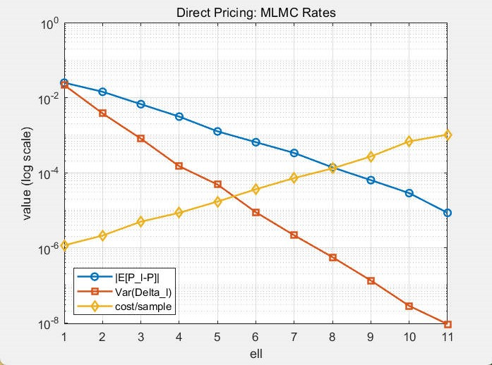
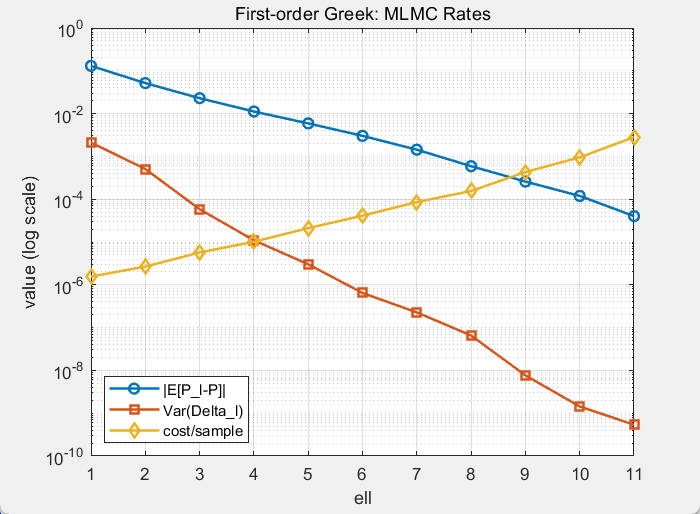
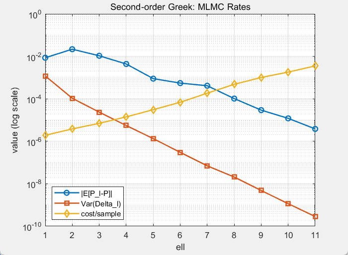
Figure 5: Multilevel bias, variance, and cost for the pricing estimator (left), first-order Greek estimator (middle), and second-order Greek estimator (right)..
| \(B_1\) | \(B_2\) | \(B_3\) | \(B_4\) | \(B_5\) | \(B_6\) | \(B_7\) | \(B_8\) | \(B_9\) | \(B_{10}\) | Mean | |
|---|---|---|---|---|---|---|---|---|---|---|---|
| \(\alpha\) | 1.087 | 1.188 | 1.050 | 1.286 | 1.291 | 1.135 | 1.107 | 1.012 | 1.033 | 1.257 | 1.145 |
| \(\beta\) | 2.008 | 2.053 | 1.993 | 2.043 | 2.075 | 2.065 | 2.045 | 2.075 | 2.042 | 2.057 | 2.045 |
| \(\gamma\) | 0.891 | 0.999 | 0.990 | 0.996 | 0.987 | 1.008 | 0.999 | 0.996 | 1.003 | 1.006 | 0.987 |
| \(B_1\) | \(B_2\) | \(B_3\) | \(B_4\) | \(B_5\) | \(B_6\) | \(B_7\) | \(B_8\) | \(B_9\) | \(B_{10}\) | Mean | |
|---|---|---|---|---|---|---|---|---|---|---|---|
| \(\alpha\) | 1.152 | 1.071 | 1.174 | 1.054 | 1.071 | 1.090 | 1.104 | 1.050 | 1.370 | 1.045 | 1.118 |
| \(\beta\) | 2.057 | 2.027 | 2.074 | 1.998 | 1.896 | 2.036 | 1.962 | 1.898 | 2.080 | 1.972 | 2.000 |
| \(\gamma\) | 1.004 | 0.996 | 0.995 | 0.997 | 1.000 | 1.002 | 1.000 | 0.992 | 1.000 | 0.995 | 0.998 |
| \(B_1\) | \(B_2\) | \(B_3\) | \(B_4\) | \(B_5\) | \(B_6\) | \(B_7\) | \(B_8\) | \(B_9\) | \(B_{10}\) | Mean | |
|---|---|---|---|---|---|---|---|---|---|---|---|
| \(\alpha\) | 1.101 | 0.914 | 0.970 | 0.872 | 1.041 | 1.076 | 1.061 | 0.984 | 0.991 | 0.998 | 1.001 |
| \(\beta\) | 2.037 | 2.067 | 2.012 | 2.000 | 2.025 | 2.071 | 2.014 | 2.009 | 2.083 | 2.059 | 2.038 |
| \(\gamma\) | 0.993 | 0.980 | 0.997 | 0.992 | 0.994 | 1.006 | 1.006 | 0.996 | 1.004 | 0.996 | 0.996 |
The empirical rates shown in Figure 5 and Tables 2–4 report the estimated multilevel exponents for the direct pricing estimator, the first-order Greek estimator, and the second-order Greek estimator.
For the direct pricing estimator, the averaged exponents over ten independent realizations of the backward Brownian motion are \[\begin{align} \alpha=1.145,\quad \beta=2.045,\quad \gamma=0.987. \end{align}\] The first-order Greek estimator gives \[\begin{align} \alpha=1.118,\quad \beta=2.000,\quad \gamma=0.998, \end{align}\] while the second-order Greek estimator gives \[\begin{align} \alpha=1.001,\quad \beta=2.038,\quad \gamma=0.996. \end{align}\]
Across all three estimators, the variance and cost exponents are particularly stable with respect to the realization of the backward Brownian motion. Moreover, the estimated exponents remain close to \[\begin{align} (\alpha,\beta,\gamma)=(1,2,1), \end{align}\] which provides strong numerical evidence for the expected multilevel scaling relations \[\begin{align} \alpha=1, \quad \beta=2, \quad \gamma=1. \end{align}\] These results are in excellent agreement with the theoretical predictions obtained from the global strong-error framework and the associated Forward–Backward Taylor schemes developed in Section 5. Consequently, the assumptions required by Theorem 3 and Corollary 1 are numerically supported.
7 Discussion and Future Work↩︎
In this paper, we developed a quantum-accelerated multilevel Monte Carlo (QA-MLMC) framework for stochastic partial differential equations (SPDEs) arising from stochastic-environment financial models. The main idea is to exploit the BDSDE representation of the SPDE solution to reformulate pricing and sensitivity estimation as conditional and nested expectation estimation problems. These expectation problems can then be estimated by QA-MLMC, leading to quadratic quantum speedups for derivative pricing and Greek estimation in stochastic environments.
The proposed framework contains two main components. First, for a fixed realization of the backward Brownian motion, we construct a conditional QA-MLMC estimator for the SPDE quantity of interest. Second, for quantities involving an additional average over the random environment, we develop a nested QA-MLMC estimator. Under the multilevel assumptions on bias, variance, and cost, these estimators achieve quantum sampling complexity of order \[\widetilde{\mathcal{O}}(\epsilon^{-1}),\] for an additive error tolerance \(\epsilon\). We also show that the same algorithmic structure applies not only to prices, but also to first-order and second-order Greeks.
A key numerical ingredient is the Forward–Backward Taylor scheme developed in this work. Unlike discretization methods that eliminate the forward Brownian randomness through conditional expectations at each time step, the Forward–Backward Taylor discretization keeps the joint pathwise dependence on the forward and backward Brownian motions. This feature is essential for constructing coupled level differences in the conditional multilevel estimator. The strong-error order one convergence results for pricing and Greek estimators provide the numerical foundation for the complexity analysis of the proposed quantum algorithms.
There are several natural directions for future work. First, although the present paper focuses on SPDEs arising from stochastic-environment financial models, the conditional and nested estimation structure is more general. It would be interesting to extend the proposed QA-MLMC framework to broader classes of SPDEs and stochastic systems with common noise, random coefficients, or random media, where BDSDE-type representations can be used to connect SPDE solutions with expectation estimation problems.
Second, the Forward–Backward Taylor discretization introduced in this work suggests several further numerical developments. One direction is to construct higher-order or adaptive forward–backward schemes that remain compatible with conditional multilevel couplings. Another is to analyze such schemes under weaker regularity assumptions, more general noise structures, or path-dependent functionals. A better understanding of the relation between strong convergence, level variance, and sample cost would also help optimize the resulting MLMC and QA-MLMC complexity.
Finally, the nested estimator developed here could be extended to more general nested or nonlinear quantities, such as risk measures and multi-layer conditional expectations. These problems arise naturally in financial applications and in stochastic systems with random environments, and provide a promising setting for further applications of quantum computing.
JPL acknowledges support from Quantum Science and Technology–National Science and Technology Major Project (Grant No. 2024ZD0300500), Excellent Young Scientists Fund Program, start-up funding from Tsinghua University and Beijing Institute of Mathematical Sciences and Applications. Z.L. was supported by the Beijing Natural Science Foundation Key Program (Grant No. Z220002). R.L. and Z.L. were supported by BMSTC and ACZSP (Grant No. Z221100002722017).
Supplementary Materials
8 Terminal-value SPDE and Its BDSDE Representation↩︎
It is well known that the Feynman-Kac formula provides a classical probabilistic representation for solutions of linear parabolic PDEs [76]. Given a terminal-value problem of the form \[\partial_t u(t,x) + \mathcal{L} u(t,x) - r(t,x)u(t,x) + F(t,x) = 0, \quad u(T,x)=G(x),\] the Feynman–Kac formula represents the solution \(u(t,x)\) as the conditional expectation of a functional of the solution to an associated SDE. More precisely, \(u(t,x)\) can be written as \[u(t,x)=\mathbb{E}\left[\Phi\left(X^{t,x}_{T}\right)\right],\] where \(X^{t,x}\) solves the SDE whose infinitesimal generator coincides with the differential operator \(\mathcal{L}\).
An important extension of the Feynman-Kac framework was achieved through the theory of backward stochastic differential equations (BSDEs). The seminal work of Pardoux and Peng established that BSDEs provide probabilistic representations for semilinear terminal-value PDEs [17], [18]. In particular, [22] discusses applications of BSDEs in mathematical finance, including the pricing of European options.
However, When the evolution equation contains an additional noise term of the form \(G(t,x)\mathrm{d}W_t\), the solution becomes a stochastic process in both time and space, leading to a stochastic partial differential equation. In this setting, neither the classical Feynman–Kac formula nor the BSDE framework is applicable.
Backward doubly stochastic differential equations (BDSDEs) [25], [64] were introduced precisely to overcome this limitation. By incorporating an additional backward Itô integral with respect to a time-reversed Brownian motion, BDSDEs extend the BSDE framework and provide a rigorous probabilistic representation for terminal-value SPDEs.
In contrast to classical BSDEs, which are associated with deterministic or random-coefficient partial differential equations, BDSDEs involve two sources of randomness: a forward Brownian motion and a backward stochastic integral. This additional backward component allows BDSDEs to faithfully capture the intrinsic randomness of SPDE solutions while preserving the backward-in-time structure imposed by the terminal condition.
Our goal is to give a probabilistic representation for the solution of the quasilinear backward SPDEs: \[\label{eq:SPDE40with32BDSDE41} \begin{cases} \partial_t u(t,x) = \left[\mathcal{L}u(t,x) + f\left(t,x,u(t,x),(\sigma^\top\nabla u)(t,x)\right)\right]\,\mathrm{d}t + h(t,x,u(t,x),(\sigma^\top\nabla u)(t,x))\,\mathrm{d}B_t,\quad t\in[0,T],\\ u(T,x)=G(x). \end{cases}\tag{50}\] There \(u:\mathbb{R_+}\times \mathbb{R}^d\rightarrow \mathbb{R}^k\) and \(\mathcal{L}u=\left( Lu_1,\cdots ,Lu_k \right)^\top\) with \(L=\frac{1}{2}\sum\limits_{i,j=1}^d(\sigma\sigma^\top)_{ij}\frac{\partial^2}{\partial x_i\partial x_j}+\sum\limits_{i=1}^db_i\frac{\partial}{\partial x_i}.\) Alternatively, we can write the SPDE 50 in the integral form \[\begin{align} \label{eq:SPDE40with32BDSDE41-integral} u(t,x)=G(x)+\int_t^T \left[\mathcal{L}u(s,x) + f\left(s,x,u(s,x),(\sigma^\top\nabla u)(s,x)\right)\right]\,\mathrm{d}s + \int_t^T h(s,x,u(s,x),(\sigma^\top\nabla u)(s,x))\mathrm d \overleftarrow{B}_s. \end{align}\tag{51}\] The backward Itô integral with respect to \(\mathrm d \overleftarrow{B}_s\) is defined as \[\begin{align} \int_t^T \phi(s) \mathrm d \overleftarrow{B}_s := \int_0^{T-t} \phi_{T-s}\,\mathrm{d}B_s', \end{align}\] where \(B_s' = B_T - B_{T-s}\) is the time-reversed Brownian motion. Equivalently, for any partition \(t=t_0<\cdots<t_n=T\), \[\begin{align} \int_t^T \phi(s)\mathrm d \overleftarrow{B}_s = \lim_{|\Pi|\to 0}\sum_{i=0}^{n-1} \phi_{t_{i+1}}\left(B_{t_i}-B_{t_{i+1}}\right), \end{align}\] with convergence in \(L^2(\Omega)\).
The connection with BDSDEs is obtained as follows. For each \((t,x)\in\mathbb{R}_+\times \mathbb{R}^d\), let \(\{X_s^{t,x};t\leq s\leq T\}\) be the solution of the SDE: \[\label{eq:SDE40with32BDSDE41} \begin{cases} \mathrm{d}X_s^{t,x}=b(X_s^{t,x})\,\mathrm{d}s +\sigma(X_s^{t,x})\,\mathrm{d}W_s,\quad s\in[t,T],\\ X_t^{t,x}=x. \end{cases}\tag{52}\] Assume that the SPDE 50 has a classical solution. Then the couple \(\left(Y_s^{t,x},Z_s^{t,x}\right)\) where \[\begin{align} Y_s^{t,x}=u(s,X_s^{t,x}),\quad Z_s^{t,x}=(\sigma^\top\nabla u)(s,X_s^{t,x}) \end{align}\] verify the following BDSDE: \[\begin{align} \label{eq:BDSDE} Y_s^{t,x}=G(X_T^{t,x})+\int_s^T f(r,X_r^{t,x},Y_r^{t,x},Z_r^{t,x})\,\mathrm{d}r +\int_s^T h(r,X_r^{t,x},Y_r^{t,x},Z_r^{t,x})\mathrm d \overleftarrow{B}_r-\int_s^T Z_r^{t,x}\,\mathrm{d}W_r,\quad t\leq s\leq T, \end{align}\tag{53}\] or alternatively \[\label{eq:BDSDE-d} \begin{cases} \mathrm{d}Y_s^{t,x}= - f(s,X_s^{t,x},Y_s^{t,x},Z_s^{t,x})\,\mathrm{d}s - h(s,X_s^{t,x},Y_s^{t,x},Z_s^{t,x})\mathrm d \overleftarrow{B}_s + Z_s^{t,x}\,\mathrm{d}W_s, \quad s\in[t,T],\\ Y_T^{t,x}=G(X_T^{t,x}). \end{cases}\tag{54}\]
In the following, based on [25], [64], we provide a more detailed exposition of results related to BDSDEs.
8.0.0.1 Fundamentals of BDSDEs
Let \((\Omega,\mathcal{F},\mathbb{P})\) be a probability space and \(T>0\) be a fixed terminal time. Let \(\{W_{t}, 0\leq t\leq T\}\) and \(\{B_{t},0\leq t\leq T\}\) be two mutually independent standard Brownian motion processes with values in \(\mathbb{R}^{d}\) and in \(\mathbb{R}^{l}\), respectively. For each \(t\in [0,T]\), we define \[\begin{align} \mathcal{F}_{t} := \mathcal{F}_{0,t}^{W} \vee \mathcal{F}_{t,T}^{B}, \end{align}\] where for any process \(\{\eta_{t}\}, \;\mathcal{F}_{s,t}^{\eta}=\sigma\{\eta_{r}-\eta_{s};s\leq r\leq t\}\vee \mathcal{N}\) and \(\mathcal{N}\) is the class of \(\mathbb{P}\)-null sets of \(\mathcal{F}\). Note that the collection \(\{ \mathcal{F}_{t}; t\in[0,T] \}\) is neither increasing nor decreasing, and it does not constitute a filtration.
We recall some notation from Pardoux and Peng [25]. For \(k\in\mathbb{N}\), we denote by \(C^k(\mathbb{R}^p;\mathbb{R}^q)\) the space of \(C^k\) functions from \(\mathbb{R}^p\) to \(\mathbb{R}^q\), by \(C^k_b(\mathbb{R}^p;\mathbb{R}^q)\) the subspace of functions whose partial derivatives up to order \(k\) are bounded, and by \(C^k_p(\mathbb{R}^p;\mathbb{R}^q)\) the space of functions whose partial derivatives up to order \(k\) have at most polynomial growth at infinity.
Let \(M^{2}([0,T]; \mathbb{R}^{n})\) be the set of \(n\)-dimensional jointly measurable stochastic processes \(\{ \varphi_{t}; t\in[0,T] \}\) which
satisfy:
(i) \(\|\varphi \|_{M^{2}}^{2} =\mathbb{E}\left[\int_0^T |\varphi_{t}|^{2} \mathrm dt\right]<\infty\);
(ii) \(\varphi_{t}\) is \(\mathcal{F}_{t}\)-measurable for a.e. \(t\in[0,T].\)
Similarly, let \(S^{2}([0,T]; \mathbb{R}^{n})\) be the set of \(n\)-dimensional continuous stochastic processes, which satisfy:
(i) \(\|\varphi \|_{S^{2}}^{2} =\mathbb{E}\left[\sup\limits_{0\leq t\leq T} |\varphi_{t}|^{2}\right]<\infty\);
(ii) \(\varphi_{t}\) is \(\mathcal{F}_{t}\)-measurable for a.e. \(t\in[0,T].\)
Assumption 1. Assume that \[\begin{align} f& : \Omega \times [0,T] \times \mathbb{R}^{k} \times \mathbb{R}^{k \times d} \to \mathbb{R}^{k},\\ h &: \Omega \times [0,T] \times \mathbb{R}^{k} \times \mathbb{R}^{k \times d} \to \mathbb{R}^{k \times l}, \end{align}\] are jointly measurable and such that for any fixed \((y,z)\), \[f(\cdot,\cdot,y,z)\in M^{2}([0,T];\mathbb{R}^{k}),\quad h(\cdot,\cdot,y,z)\in M^{2}([0,T];\mathbb{R}^{k \times l}).\] We assume moreover that there exist some constants \(c>0\) and \(0< \alpha<1\) such that for every \((\omega,t)\in \Omega\times[0,T]\) and \((y_1,z_1),(y_2,z_2)\in \mathbb{R}^{k}\times\mathbb{R}^{k\times d},\) the following inequalities hold: \[\begin{align} | f(t,y_1,z_1)-f(t,y_2,z_2)|^{2} &\leq c\left(| y_1-y_2|^{2}+\| z_1-z_2\|^{2}\right), \label{eq:f95lipschitz}\\ \|h(t,y_1,z_1)-h(t,y_2,z_2)\|^{2} &\leq c| y_1-y_2|^{2}+\alpha \| z_1-z_2\|^{2}. \label{eq:h95lipschitz} \end{align}\] {#eq: sublabel=eq:eq:f95lipschitz,eq:eq:h95lipschitz} Here \(|y|\) denotes the Euclidean norm and \(\|z\|^{2} = \operatorname{Tr}(z z^{*}).\)
Remark 7. Note that, in the SPDE 50 and the BDSDE 53 , the coefficient functions under consideration are of the form \[\begin{align} f &: [0,T]\times \mathbb{R}^d \times \mathbb{R}^k \times \mathbb{R}^{k\times d} \to \mathbb{R}^k,\\ h &: [0,T]\times \mathbb{R}^d \times \mathbb{R}^k \times \mathbb{R}^{k\times d} \to \mathbb{R}^{k\times \ell}. \end{align}\]
Let \(b\in C_b^3(\mathbb{R}^d;\mathbb{R}^d)\) and \(\sigma\in C_b^3(\mathbb{R}^d;\mathbb{R}^{d\times d})\). For each \(t\in[0,T]\) and \(x\in\mathbb{R}^d\), we denote by \(\{X_s^{t,x};\, t\le s\le T\}\) the unique strong solution of the SDE 52 . Then the two formulations are then naturally linked through the forward diffusion process by adopting the shorthand notation \[f(s,y,z) = f\left(s, X_s^{t,x}, y, z\right), \quad h(s,y,z) = h\left(s, X_s^{t,x}, y, z\right).\] Moreover, we assume that for any \(s\in[0,T]\), \((x,y,z)\rightarrow \left(f(s,x,y,z),h(s,x,y,z)\right)\) is of class \(C^3\).
Proposition 12. (Theorem 1.1 in [25] ) Under the Assumption 1, the BDSDE \[\begin{align} Y_t=\xi+\int_t^Tf(s,Y_s,Z_s)\,\mathrm{d}s +\int_t^Th(s,Y_s,Z_s)\mathrm d \overleftarrow{B}_s -\int_t^T Z_s\,\mathrm{d}W_s,\quad 0\leq t\leq T, \end{align}\] has unique solution \[(Y,Z)\in S^2([0,T];\mathbb{R}^k)\times M^2([0,T];\mathbb{R}^{k\times d})\] for any \(\xi\in L^2\left(\Omega,\mathcal{F}_T,\mathbb{P};\mathbb{R}^k\right)\).
Assumption 2. There exists a constant \(c>0\) such that, for all \((t,y,z)\in[0,T]\times \mathbb{R}^k\times\mathbb{R}^{k\times d}\), \[h(t,y,z)h(t,y,z)^{*} \leq zz^{*}+c\left(\|h(t,0,0)\|^{2}+|y|^{2}\right)I.\]
Assumption 3. For all \(t\in[0,T]\), \(x\in\mathbb{R}^d\), \(y\in\mathbb{R}^k\) and \(z,\theta\in\mathbb{R}^{k\times d}\), it holds that \[h_z'(t,x,y,z)\,\theta\theta^{*}\,h_z'(t,x,y,z)^{*} \leq \theta\theta^{*}.\]
The following two theorems establish the connection between solutions of BDSDEs and SPDEs in the general setting.
Theorem 5 (Theorem 3.1 in [25]). Assume that \(f\) and \(h\) satisfy Assumptions 1 and 2, and that \(G\in C^2\). Let \(u\) be a solution to the SPDE 50 . Then \[u(t,x)=Y_t^{t,x},\] where \(\{(Y_s^{t,x},Z_s^{t,x});\, t\leq s\leq T\}\) is the unique solution of the BDSDE 53 .
Theorem 6 (Theorem 3.2 in [25]). Let \(f\), \(G\) and \(h\) satisfy Assumption 1, 2 and 3, then \[\{u(t,x)\triangleq Y_t^{t,x};0\leq t\leq T,x\in\mathbb{R}^d\}\] is the unique classical solution of the system of backward SPDEs 52 , where \(\{(Y_s^{t,x},Z_s^{t,x});t\leq s\leq T\}\) is the unique solution of the BDSDE 53 .
8.0.0.2 Linear SPDEs and BDSDEs
In our applications of SPDEs, we are mainly interested in the linear case. Therefore, following [64], we present the linear setting that will be used in this work.
In the linear setting, consider \[\begin{align} f(t,x,y,z)=F(t,x)+c(t)y+\widetilde{c}(t)z,\quad h(t,x,y,z)=H(t,x)+d(t)y, \end{align}\] where \(c,\widetilde{c}\) are bounded deterministic functions. Then the BDSDE 53 becomes \[\begin{align} \label{eq:linear32BDSDE} Y_s^{t,x}=G(X_T^{t,x})+\int_s^T \left[F(r,X_r^{t,x})+c(r)Y_r^{t,x}+\widetilde{c}(r)Z_r^{t,x}\right]\,\mathrm{d}r +\int_s^T \left[H(r,X_r^{t,x})+d(r)Y_r^{t,x}\right]\mathrm d \overleftarrow{B}_r- \int_s^T Z_r^{t,x}\,\mathrm{d}W_r,\quad t\leq s\leq T, \end{align}\tag{55}\] and the SPDE 50 becomes \[\label{eq:linear32SPDE40with32BDSDE41} \begin{cases} \mathrm{d} u(t,x) = \Bigl[\mathcal{L}u(t,x) + F(t,x) + c(t)u(t,x) + \widetilde{c}(t)(\sigma^\top\nabla u)(t,x)\Bigr]\,\mathrm{d}t + \Bigl[H(t,x)+d(t)u(t,x)\Bigr]\,\mathrm{d}B_t,\quad t\in[0,T],\\ u(T,x)=G(x). \end{cases}\tag{56}\]
Proposition 13 (Linear BDSDE representation, Proposition 2.1 in [64]). Assume that \(G\in C_p^3(\mathbb{R}^d)\) and that \(F, H\in C_b^3([0,T]\times\mathbb{R}^d)\). Let \(\{X_s^{t,x};t\leq s\leq T\}\) be the solution of the SDE 52 and define the stochastic exponential \(\Phi(s,r)\) as \[\begin{align} \Phi(s,\tau)=\exp\left(\int_s^\tau c(r)\,\mathrm{d}r +\int_s^\tau d(r)\mathrm d \overleftarrow{B}_r +\int_s^\tau \widetilde{c}(r)\,\mathrm{d}W_r -\frac{1}{2}\int_s^\tau\left(|\widetilde{c}(r)|^2-|d(r)|^2\right)\mathrm d r\right). \end{align}\] Then,
(i)The unique solution \(\{(Y_s^{t,x},Z_s^{t,x});\, t\le s\le T\}\) of 55 is given by \[\begin{align} Y_s^{t,x} = \Phi(s,T) G\bigl(X_T^{t,x}\bigr) + \int_s^T \Phi(s,r) \Bigl( F\bigl(r,X_r^{t,x}\bigr) + d(r) H\bigl(r,X_r^{t,x}\bigr) \Bigr)\,\mathrm{d}r + \int_s^T \Phi(s,r) H\bigl(r,X_r^{t,x}\bigr) \mathrm d \overleftarrow{B}_r - \int_s^T \Phi(s,r) Z_r^{t,x}\,\mathrm{d}W_r , \end{align}\] and it can be written as \[\begin{align} Y_s^{t,x}=\mathbb{E}\left[\Phi(s,T)G(X_T^{t,x}) +\int_s^T\Phi(s,r)\left(F(r,X_r^{t,x})+d(r) H(r,X_r^{t,x})\right)\,\mathrm{d}r +\int_s^T\Phi(s,r)H(r,X_r^{t,x})\mathrm d \overleftarrow{B}_r\,|\,\mathcal{F}_{t,s}^W\vee \mathcal{F}_{t,T}^B \right]. \end{align}\]
(ii)The SPDE 56 has a unique solution \(u\) and it can be written as \[\begin{align} u(t,x)=\mathbb{E}\left[\Phi(t,T)G(X_T^{t,x}) +\int_t^T\Phi(t,r)\left(F(r,X_r^{t,x})+d(r) H(r,X_r^{t,x})\right)\,\mathrm{d}r +\int_t^T\Phi(t,r)H(r,X_r^{t,x})\mathrm d \overleftarrow{B}_r\,|\,\mathcal{F}_{t,T}^B \right]. \end{align}\]
9 Proofs for the Strong-error Framework↩︎
This appendix collects the technical proofs underlying the strong-error analysis developed in Section 5. The corresponding discretization operators are introduced in the main text, and here we establish the local consistency, strong-error, and accumulated stability estimates required for the global strong-error order one convergence results.
9.0.0.1 Notation and conventions.
Throughout this appendix, \(C\) and \(C_q\) denote generic constants, independent of the time step \(h\), whose values may change from line to line. Whenever a uniform grid is used, we write \[t_k=t_0+kh,\quad k=0,\ldots,N,\quad t_N=T,\] with \(h=(T-t_0)/N\). For simplicity, denote \[A(r,x):=F(r,x)+d(r)H(r,x).\]
Unless explicitly stated otherwise, all \(L^p\) norms are taken with respect to the joint law of the Brownian motions \((W,B)\). That is, \[\|\cdot\|_{L^p}:=\|\cdot\|_{L^p_{W,B}} .\] When a fixed realization of the backward Brownian motion \(B\) is considered, we write the conditional norm explicitly as \(L_W^p\).
9.0.0.2 Forward–backward information and martingale estimates.
In the BDSDE setting, the natural information at a grid point \(t_k\) consists of the forward \(W\)-information up to \(t_k\) and the backward \(B\)-information from \(t_k\) to \(T\). At the grid level we write this information as \[\mathcal{G}_k := \sigma(W_{t_0},\ldots,W_{t_k}) \vee \sigma(B_{t_k}-B_{t_m}: k\le m\le N) \vee\mathcal{N} .\] The family \((\mathcal{G}_k)_{k=0}^N\) is not a filtration in the ordinary increasing-time sense: the \(W\)-part is increasing in \(k\), while the \(B\)-part is decreasing in \(k\). Thus, when estimating accumulated local fluctuations below, we do not regard \((\mathcal{G}_k)\) itself as a filtration.
Instead, each martingale-type contribution is treated by splitting it into its forward and backward parts. The \(W\)-terms are estimated as ordinary forward martingale differences and the \(B\)-terms are estimated as backward martingale differences, or equivalently as ordinary martingale differences after introducing the reversed Brownian motion \[\widehat B_u:=B_T-B_{T-u},\quad 0\le u\le T .\] The Burkholder–Davis–Gundy estimates used below are always applied in this split sense, and the resulting forward and reversed-time estimates are combined by the triangle and Minkowski inequalities.
9.0.0.3 A joint-to-conditional estimate.
Most of the strong-error estimates in this appendix are first proved under the joint law of the two Brownian motions \((W,B)\). However, in conditional setting, we need to interpret the estimate after fixing a realization of the backward Brownian motion \(B\), so that the remaining randomness comes only from the forward Brownian motion \(W\). The following elementary lemma provides this passage from joint \(L^p_{W,B}\)-bounds to conditional \(L^p_W\)-bounds for \(\mathbb{P}_B\)-almost every realization of \(B\).
The point of the lemma is that a deterministic joint strong-error estimate on a sequence of dyadic time steps can be converted into an almost-sure-in-\(B\) conditional estimate, at the cost of a harmless logarithmic-type factor. More precisely, if an error family satisfies \[\mathbb{E}_{W,B} \left[ \sup_{0\le k\le N_\ell} |\Pi_{\ell,k}|^p \right] \le C_p2^{-p\ell},\] then for almost every fixed \(B\), the conditional \(W\)-error has the same dyadic decay rate up to the factor \((1+\ell)^a\), with a finite random constant depending on \(B\). This loss is mild and is sufficient for the pathwise-in-\(B\) estimates used below.
Lemma 2. Let \(p\ge2\). Assume that we are given a jointly measurable family of random variables \[\{\Pi_{\ell,k}\}_{0\le k\le N_\ell,\,\ell\ge1}\] depending on both \(W\) and \(B\), such that \[\mathbb{E}_{W,B} \left[ \sup_{0\le k\le N_\ell} \left| \Pi_{\ell,k} \right|^p \right] \le C_p2^{-p\ell}, \quad \ell\ge1.\] Then, for every \(a>1\), there exists a finite random constant \(C_{p,a}(B)<\infty\) for \(\mathbb{P}_B\)-almost every realization of \(B\), such that for all \(\ell\ge1\), \[\mathbb{E}_W \left[ \sup_{0\le k\le N_\ell} \left| \Pi_{\ell,k} \right|^p \,\middle|\,B \right] \le C_{p,a}(B)(1+\ell)^a2^{-p\ell}.\]
Proof. For each \(\ell\ge1\), define \[V_\ell^{(p)}(B) := \mathbb{E}_W \left[ \sup_{0\le k\le N_\ell} \left| \Pi_{\ell,k} \right|^p \,\middle|\,B \right].\] Then \[\mathbb{E}_B\left[V_\ell^{(p)}(B)\right] = \mathbb{E}_{W,B} \left[ \sup_{0\le k\le N_\ell} \left| \Pi_{\ell,k} \right|^p \right] \le C_p2^{-p\ell}.\]
Fix \(a>1\) and define \[C_{p,a}(B) := \sum_{\ell=1}^{\infty} \frac{2^{p\ell}}{(1+\ell)^a} V_\ell^{(p)}(B).\] Since all terms in the series are nonnegative, \[\mathbb{E}_B\left[C_{p,a}(B)\right] = \sum_{\ell=1}^{\infty} \frac{2^{p\ell}}{(1+\ell)^a} \mathbb{E}_B\left[V_\ell^{(p)}(B)\right] \le C_p \sum_{\ell=1}^{\infty} \frac{1}{(1+\ell)^a} <\infty,\] where the last inequality follows from \(a>1\). Hence \[C_{p,a}(B)<\infty\] for \(\mathbb{P}_B\)-almost every realization of \(B\).
For such a realization of \(B\), since every term in the defining series of \(C_{p,a}(B)\) is nonnegative, we have, for every \(\ell\ge1\), \[\frac{2^{p\ell}}{(1+\ell)^a} V_\ell^{(p)}(B) \le C_{p,a}(B).\] Therefore, \[V_\ell^{(p)}(B) \le C_{p,a}(B)(1+\ell)^a2^{-p\ell},\] i.e. \[\mathbb{E}_W \left[ \sup_{0\le k\le N_\ell} \left| \Pi_{\ell,k} \right|^p \,\middle|\,B \right] \le C_{p,a}(B)(1+\ell)^a2^{-p\ell},\] for all \(\ell\ge1\) and for \(\mathbb{P}_B\)-almost every realization of \(B\). ◻
9.1 Direct Pricing Estimator↩︎
9.1.0.1 Proof of Proposition 3
Proposition 1 (Strong-error order for the direct pricing payoff). Fix \((t,x)\in[0,T]\times\mathbb{R}^d\) and a uniform grid \(\{t_k\}_{k=0}^N\) with \(h=(T-t)/N\). Let \[\begin{align} P_{t_k}=\Phi(t,t_k)G\left(X_{t_k}^{t,x}\right)+Y_{t_k}, \end{align}\] where \(Y_{t_k}\) is the exact accumulated payoff \[\begin{align} Y_{t_k}=\int_t^{t_k}\Phi(t,r)\left(F(r,X_r^{t,x})+d(r)H(r,X_r^{t,x})\right)\,\mathrm{d} r +\int_t^{t_k}\Phi(t,r)H(r,X_r^{t,x})\,\mathrm d \overleftarrow{B}_r. \end{align}\]
Let \(\left\{\left(X_k^{(h)},\Phi_k^{(h)}\right)\right\}_{k=0}^N\) be the approximations generated by the schemes \(S_X,S_\Phi\) as in Definition 1, 2 and define \[\begin{align} Y_{k+1}^{(h)} =& Y_k^{(h)} + \mathcal{S}_{\mathrm{int}} \left( \Phi_k^{(h)}, X_k^{(h)},t_k,h; \Delta W_{t_k}, \Delta\overleftarrow B_{t_k} \right), \quad Y_0^{(h)}=0,\\ P_k^{(h)}=&\Phi^{(h)}_k G\left(X_k^{(h)}\right)+Y_k^{(h)}. \end{align}\]
Assume:
The strong-error orders of \(\mathcal{S}_X\), \(\mathcal{S}_\Phi\) and \(\mathcal{S}_{\mathrm{int}}\) are \(p_X,p_\Phi,p_{\mathrm{int}}\) respectively. Moreover, \(\mathcal{S}_{\mathrm{int}}\) satisfies the accumulated stability estimate defined in Definition 4.
There exists \(M>0\), independent of \(h\), such that \(\Phi_k^{(h)}\) and \(G(X_{t_k}^{t,x})\) are uniformly bounded in \(L^{4}_{W,B}\) by \(M\).
\(G\) is globally Lipschitz, i.e., there exists \(L_G>0\) such that \(|G(x)-G(y)|\leq L_G|x-y|\).
Then the payoff approximation satisfies the joint strong-error bound \[\begin{align} \left\| \sup_{0\leq k\leq N} \left| P_{t_k}-P^{(h)}_k \right| \right\|_{L^2} = \mathcal{O}(h^p), \quad p=\min\{p_X,p_\Phi,p_{\mathrm{int}}\}. \end{align}\]
Proof. First, for each \(0\le k\le N\), we have \[\begin{align} P_{t_k}-P_k^{(h)} =& \left( \Phi(t,t_k)G\left(X_{t_k}^{t,x}\right)+Y_{t_k} \right) - \left( \Phi_k^{(h)}G\left(X_k^{(h)}\right)+Y_k^{(h)} \right)\\ =& \left(\Phi(t,t_k)-\Phi_k^{(h)}\right) G\left(X_{t_k}^{t,x}\right) + \Phi_k^{(h)} \left( G\left(X_{t_k}^{t,x}\right)-G\left(X_k^{(h)}\right) \right)+ \left(Y_{t_k}-\widetilde{Y}_k^{(h)}\right) + \left(\widetilde{Y}_k^{(h)}-Y_k^{(h)}\right). \end{align}\]
Taking the supremum over \(0\le k\le N\) and then using the triangle inequality and Hölder’s inequality, we obtain \[\begin{align} & \left\| \sup_{0\le k\le N} \left| P_{t_k}-P_k^{(h)} \right| \right\|_{L^2}\\ \le& \left\| \sup_{0\le k\le N} \left| \left(\Phi(t,t_k)-\Phi_k^{(h)}\right) G\left(X_{t_k}^{t,x}\right) \right| \right\|_{L^2}+ \left\| \sup_{0\le k\le N} \left| \Phi_k^{(h)} \left( G\left(X_{t_k}^{t,x}\right)-G\left(X_k^{(h)}\right) \right) \right| \right\|_{L^2}\\ &+ \left\| \sup_{0\le k\le N} \left| Y_{t_k}-\widetilde{Y}_k^{(h)} \right| \right\|_{L^2} + \left\| \sup_{0\le k\le N} \left| \widetilde{Y}_k^{(h)}-Y_k^{(h)} \right| \right\|_{L^2}\\ \le& \left\| \sup_{0\le k\le N} \left| \Phi(t,t_k)-\Phi_k^{(h)} \right| \right\|_{L^4} \left\| \sup_{0\le k\le N} \left| G\left(X_{t_k}^{t,x}\right) \right| \right\|_{L^4}+ \left\| \sup_{0\le k\le N} \left| \Phi_k^{(h)} \right| \right\|_{L^4} \left\| \sup_{0\le k\le N} \left| G\left(X_{t_k}^{t,x}\right)-G\left(X_k^{(h)}\right) \right| \right\|_{L^4}+ C_{\mathrm{int}}h^{p_{\mathrm{int}}}\\ &+ L_{\mathrm{int}} \bigg( \left\| \sup_{0\le j\le N} \left| \Phi(t,t_j)-\Phi_j^{(h)} \right| \right\|_{L^4} + \left\| \sup_{0\le j\le N} \left| X_{t_j}^{t,x}-X_j^{(h)} \right| \right\|_{L^4} \bigg). \end{align}\] By the moment assumption and the Lipschitz continuity of \(G\), \[\begin{align} \left\| \sup_{0\le k\le N} \left| P_{t_k}-P_k^{(h)} \right| \right\|_{L^2} \le& M \left\| \sup_{0\le k\le N} \left| \Phi(t,t_k)-\Phi_k^{(h)} \right| \right\|_{L^4} + ML_G \left\| \sup_{0\le k\le N} \left| X_{t_k}^{t,x}-X_k^{(h)} \right| \right\|_{L^4}\\ &+ C_{\mathrm{int}}h^{p_{\mathrm{int}}} + L_{\mathrm{int}} \bigg( \left\| \sup_{0\le j\le N} \left| \Phi(t,t_j)-\Phi_j^{(h)} \right| \right\|_{L^4} + \left\| \sup_{0\le j\le N} \left| X_{t_j}^{t,x}-X_j^{(h)} \right| \right\|_{L^4} \bigg). \end{align}\] Using the pathwise-in-time strong-error order estimates for \(S_X\) and \(S_\Phi\), we therefore get \[\begin{align} & \left\| \sup_{0\le k\le N} \left| P_{t_k}-P_k^{(h)} \right| \right\|_{L^2} \le C_\Phi(M+L_{\mathrm{int}})h^{p_\Phi} + C_X(ML_G+L_{\mathrm{int}})h^{p_X} + C_{\mathrm{int}}h^{p_{\mathrm{int}}}. \end{align}\] Hence, for all sufficiently small \(h\), \[\begin{align} \left\| \sup_{0\le k\le N} \left| P_{t_k}-P_k^{(h)} \right| \right\|_{L^2} \le C h^p, \quad p=\min\{p_X,p_\Phi,p_{\mathrm{int}}\}. \end{align}\] This proves \[\left\| \sup_{0\leq k\leq N} \left| P_{t_k}-P^{(h)}_k \right| \right\|_{L^2} = \mathcal{O}(h^{p}).\] ◻
9.1.0.2 Proof of Proposition 4
Proposition 2 (Strong error of the integral discretization). Assume that \(F,H,d,\widetilde{c}\) and the coefficients of \(X\) and \(\Phi\) are sufficiently smooth with polynomial growth, and that the corresponding moments of \(X\) and \(\Phi\) are uniformly bounded. Then the approximation generated by \[\begin{align} \widetilde{Y}_{k+1}^{(h)} = \widetilde{Y}_k^{(h)} + \mathcal{S}_{\mathrm{int}}^{\mathrm{FBT}} \left(\Phi(t,t_k),X_{t_k}^{t,x}, t_k,h;\Delta W_{t_k},\Delta\overleftarrow B_{t_k}\right), \quad \widetilde{Y}_0^{(h)}=0, \end{align}\] satisfies \[\begin{align} \left\| \sup_{0\le k\le N} \left| Y_{t_k}-\widetilde{Y}_k^{(h)} \right| \right\|_{L^q} \le Ch, \end{align}\] for every \(q\ge2\). Consequently, by Jensen’s inequality, the same estimate also holds for every \(0<q<2\). Hence \(\mathcal{S}_{\mathrm{int}}^{\mathrm{FBT}}\) has strong-error order \(1\) in the sense of Definition 3.
Proof. For \(k=0,\ldots,N-1\), write the exact one-step integral as \[\begin{align} I_k := \int_{t_k}^{t_{k+1}} \Phi(t,r)\bigl(F(r,X_r^{t,x})+d(r)H(r,X_r^{t,x})\bigr)\,\mathrm dr + \int_{t_k}^{t_{k+1}} \Phi(t,r)H(r,X_r^{t,x})\cdot \mathrm d \overleftarrow{B}_r. \end{align}\] Then, for each \(0\le n\le N\), \[\begin{align} Y_{t_n}-\widetilde{Y}_n^{(h)} = \sum_{k=0}^{n-1} \left[ I_k- \mathcal{S}_{\mathrm{int}}^{\mathrm{FBT}} \left( \Phi(t,t_k),X_{t_k}^{t,x}, t_k,h; \Delta W_{t_k},\Delta\overleftarrow B_{t_k} \right) \right]. \end{align}\]
We first record the one-step consistency decomposition. By the smoothness assumptions and the local Itô–Taylor expansions of \(X\) and \(\Phi\), for \(r\in[t_k,t_{k+1}]\), \[\begin{align} \Phi(t,r)A(r,X_r^{t,x}) =\Phi(t,t_k)A(t_k,X_{t_k}^{t,x}) +&\Phi(t,t_k) \sum_{a=1}^d \left( \nabla_xA(t_k,X_{t_k}^{t,x})^\top \sigma_{\cdot a}(X_{t_k}^{t,x})+\widetilde{c}_a(t_k)A(t_k,X_{t_k}^{t,x})\right) \left(W_r^a-W_{t_k}^a\right)\\ +&\Phi(t,t_k)\,\sum_{\alpha=1}^{\ell} d_\alpha(t_k)\, A(t_k,X_{t_k}^{t,x}) \left(B_{t_{k}}^\alpha-B_r^\alpha\right) + R_{k,r}^{D}, \end{align}\] where \(\|R_{k,r}^{D}\|_{L^q} \le C_q(r-t_k).\)
Set \(A_{k,h}^{D}:=\int_{t_k}^{t_{k+1}}R_{k,r}^{D}\,\mathrm dr\) and \[\begin{align} M_{k,h}^{D} :=& \Phi(t,t_k) \sum_{a=1}^d \left( \nabla_xA(t_k,X_{t_k}^{t,x})^\top \sigma_{\cdot a}(X_{t_k}^{t,x})+\widetilde{c}_a(t_k)A(t_k,X_{t_k}^{t,x})\right) \int_{t_k}^{t_{k+1}} \left(W_r^a-W_{t_k}^a\right)\,\mathrm dr\\ &\quad+\Phi(t,t_k)\,\sum_{\alpha=1}^{\ell} d_\alpha(t_k)\, A(t_k,X_{t_k}^{t,x}) \int_{t_k}^{t_{k+1}} \left(B_{t_{k}}^\alpha-B_r^\alpha\right)\,\mathrm dr . \end{align}\] Then \[\begin{align} \label{eq:direct-A-D-bound} \|A_{k,h}^{D}\|_{L^q}\le C_qh^2, \end{align}\tag{57}\] and \(M_{k,h}^{D}\) is a martingale-type local fluctuation in the sense of the discrete forward–backward information convention above: its \(W\)-part is a forward martingale difference and its \(B\)-part is a reverse martingale difference, equivalently a martingale difference after reversing the \(B\)-time. Moreover, \[\begin{align} \|M_{k,h}^{D}\|_{L^q} \le C_qh^{3/2}. \label{eq:direct-M-D-bound} \end{align}\tag{58}\] We have \[\begin{align} \int_{t_k}^{t_{k+1}} \Phi(t,r)A(r,X_r^{t,x})\,\mathrm dr - h\Phi(t,t_k)A(t_k,X_{t_k}^{t,x}) = A_{k,h}^{D}+M_{k,h}^{D}. \end{align}\]
Next, for the backward stochastic integral, the local expansions of \(X\), \(H\), and \(\Phi\) yield \[\begin{align} \Phi(t,r)H(r,X_r^{t,x}) = \Phi(t,t_k)H(t_k,X_{t_k}^{t,x}) &+ \Phi(t,t_k) \bigl( H_x(t_k,X_{t_k}^{t,x})\sigma(X_{t_k}^{t,x}) +\widetilde{c}(t_k)H(t_k,X_{t_k}^{t,x}) \bigr) \left(W_r-W_{t_k}\right)\\ &+ \Phi(t,t_k)d(t_k)H(t_k,X_{t_k}^{t,x}) \left(B_{t_{k}}-B_r\right) + R_{k,r}^{B}, \end{align}\] with \[\begin{align} \|R_{k,r}^{B}\|_{L^q} \le C_q\Big((r-t_k)+(r-t_k)^{1/2}h^{1/2}\Big). \label{eq:direct-backward-integrand-remainder} \end{align}\tag{59}\] Therefore, after subtracting the corresponding Forward–Backward Taylor correction terms in \(\mathcal{S}_{\mathrm{int}}^{\mathrm{FBT}}\), the one-step error has the form \[\begin{align} I_k- \mathcal{S}_{\mathrm{int}}^{\mathrm{FBT}} \left( \Phi(t,t_k),X_{t_k}^{t,x}, t_k,h; \Delta W_{t_k},\Delta\overleftarrow B_{t_k} \right) = A_{k,h}^{D}+M_{k,h}^{D}+R_{k,h}^{B}, \label{eq:direct-one-step-consistency} \end{align}\tag{60}\] where \[\begin{align} R_{k,h}^{B} := \int_{t_k}^{t_{k+1}} R_{k,r}^{B}\cdot\mathrm d \overleftarrow{B}_r. \end{align}\] Moreover, by 59 , \[\begin{align} \int_{t_k}^{t_{k+1}} \|R_{k,r}^{B}\|_{L^q}^2\,\mathrm dr \le C_qh^3. \label{eq:direct-integrated-RB-bound} \end{align}\tag{61}\]
Using 60 , we have, for every \(0\le n\le N\), \[\begin{align} Y_{t_n}-\widetilde{Y}_n^{(h)} = \sum_{k=0}^{n-1}A_{k,h}^{D} + \sum_{k=0}^{n-1}M_{k,h}^{D} + \sum_{k=0}^{n-1}R_{k,h}^{B}. \end{align}\]
We estimate the three accumulated terms separately. For the finite-variation part, by the pathwise bound \[\sup_{0\le n\le N} \left| \sum_{k=0}^{n-1}A_{k,h}^{D} \right| \le \sum_{k=0}^{N-1} |A_{k,h}^{D}|,\] and 57 , we get \[\begin{align} \left\| \sup_{0\le n\le N} \left| \sum_{k=0}^{n-1}A_{k,h}^{D} \right| \right\|_{L^q} \le \sum_{k=0}^{N-1} \|A_{k,h}^{D}\|_{L^q} \le C_qNh^2 \le C_qh. \label{eq:direct-global-A-bound} \end{align}\tag{62}\]
For the martingale-type contribution, the discrete Burkholder–Davis–Gundy inequality gives \[\begin{align} \left\| \sup_{0\le n\le N} \left| \sum_{k=0}^{n-1}M_{k,h}^{D} \right| \right\|_{L^q} &\le C_q \left\| \left( \sum_{k=0}^{N-1} |M_{k,h}^{D}|^2 \right)^{1/2} \right\|_{L^q} \notag\\ &= C_q \left\| \sum_{k=0}^{N-1} |M_{k,h}^{D}|^2 \right\|_{L^{q/2}}^{1/2} \notag\\ &\le C_q \left( \sum_{k=0}^{N-1} \|M_{k,h}^{D}\|_{L^q}^2 \right)^{1/2} \notag\\ &\le C_q(Nh^3)^{1/2} \le C_qh. \label{eq:direct-global-M-bound} \end{align}\tag{63}\] Here we used Minkowski’s inequality in \(L^{q/2}\), which is valid because \(q\ge2\).
Finally, since \[\sum_{k=0}^{n-1}R_{k,h}^{B} = \int_t^{t_n} R_r^{B,h}\cdot\mathrm d \overleftarrow{B}_r, \quad R_r^{B,h}:=R_{k,r}^{B}\quad \text{for }r\in[t_k,t_{k+1}],\] the Burkholder–Davis–Gundy inequality for backward Itô integrals yields \[\begin{align} & \left\| \sup_{0\le n\le N} \left| \sum_{k=0}^{n-1}R_{k,h}^{B} \right| \right\|_{L^q} \notag\\ \le & C_q \left\| \left( \sum_{k=0}^{N-1} \int_{t_k}^{t_{k+1}} |R_{k,r}^{B}|^2\,\mathrm dr \right)^{1/2} \right\|_{L^q} \notag\\ \le & C_q \left( \sum_{k=0}^{N-1} \int_{t_k}^{t_{k+1}} \|R_{k,r}^{B}\|_{L^q}^2\,\mathrm dr \right)^{1/2} \notag\\ \le & C_q(Nh^3)^{1/2} \le C_qh. \label{eq:direct-global-RB-bound} \end{align}\tag{64}\]
Combining 62 , 63 , and 64 , we obtain \[\begin{align} \left\| \sup_{0\le n\le N} \left| Y_{t_n}-\widetilde{Y}_n^{(h)} \right| \right\|_{L^q} \le C_qh, \quad q\ge2. \end{align}\] This proves the claimed estimate for \(q\ge2\).
For \(0<q<2\), Jensen’s inequality gives \[\begin{align} \left\| \sup_{0\le n\le N} \left| Y_{t_n}-\widetilde{Y}_n^{(h)} \right| \right\|_{L^q} \le \left\| \sup_{0\le n\le N} \left| Y_{t_n}-\widetilde{Y}_n^{(h)} \right| \right\|_{L^2} \le C_2h. \end{align}\] Hence \(\mathcal{S}_{\mathrm{int}}^{\mathrm{FBT}}\) has strong-error order \(1\) in the sense of Definition 3. ◻
9.1.0.3 Proof of Proposition 5
Proposition 3. Assume that \(F,H\) are globally Lipschitz and have at most linear growth. Moreover, assume that the coefficient \(H_x(t,x)\sigma(x)+\widetilde{c}(t)H(t,x)\) is globally Lipschitz and has at most linear growth. Assume further that the exact and numerical input processes satisfy the uniform moment bound \[\left\| \sup_{0\le j\le N} |\Phi(t,t_j)| \right\|_{L^8} + \left\| \sup_{0\le j\le N} |\Phi_j^{(h)}| \right\|_{L^8} + \left\| \sup_{0\le j\le N} |X_{t_j}^{t,x}| \right\|_{L^8} + \left\| \sup_{0\le j\le N} |X_j^{(h)}| \right\|_{L^8} <\infty .\] Then \(\mathcal{S}_{\mathrm{int}}^{\mathrm{FBT}}\) satisfies the accumulated stability condition in Definition 4. More precisely, there exists \(L_{\mathrm{int}}>0\), independent of \(h\), such that \[\begin{align} \left\| \sup_{0\leq k\leq N} \left| \widetilde{Y}_k^{(h)}-Y_k^{(h)} \right| \right\|_{L^2} \le L_{\mathrm{int}} \bigg( & \left\| \sup_{0\leq j\leq N} \left| \Phi(t,t_j)-\Phi_j^{(h)} \right| \right\|_{L^4} + \left\| \sup_{0\leq j\leq N} \left| X_{t_j}^{t,x}-X_j^{(h)} \right| \right\|_{L^4} \bigg). \end{align}\]
Proof. Set \(\Delta\Phi_j:=\Phi(t,t_j)-\Phi_j^{(h)}\) and \(\Delta X_j:=X_{t_j}^{t,x}-X_j^{(h)}\). Define \[\delta_\Phi := \left\| \sup_{0\le j\le N} |\Delta\Phi_j| \right\|_{L^4}, \quad \delta_X := \left\| \sup_{0\le j\le N} |\Delta X_j| \right\|_{L^4}, \quad \delta:=\delta_\Phi+\delta_X.\]
By the definitions of \(\widetilde{Y}_k^{(h)}\) and \(Y_k^{(h)}\), we have \[\begin{align} \widetilde{Y}_k^{(h)}-Y_k^{(h)} = \sum_{j=0}^{k-1} \Bigg[ &\mathcal{S}_{\mathrm{int}}^{\mathrm{FBT}} \left(\Phi(t,t_j),X_{t_j}^{t,x},t_j,h; \Delta W_{t_j},\Delta\overleftarrow B_{t_j}\right) - \mathcal{S}_{\mathrm{int}}^{\mathrm{FBT}} \left(\Phi_j^{(h)},X_j^{(h)},t_j,h; \Delta W_{t_j},\Delta\overleftarrow B_{t_j}\right) \Bigg]. \end{align}\]
We estimate the four contributions in \(\mathcal{S}_{\mathrm{int}}^{\mathrm{FBT}}\) separately.
First consider the time-integral term. Since \(F\) and \(H\) are globally Lipschitz with at most linear growth, and \(d\) is bounded, \(A\) is globally Lipschitz in \(x\) and has at most linear growth. Hence, using Hölder’s inequality and the uniform moment bounds, \[\begin{align} & \left\| \sup_{0\le k\le N} \left| \sum_{j=0}^{k-1} h\Big[ \Phi(t,t_j)A(t_j,X_{t_j}^{t,x}) - \Phi_j^{(h)}A(t_j,X_j^{(h)}) \Big] \right| \right\|_{L^2} \\ \le& \sum_{j=0}^{N-1} h \left\| \Phi(t,t_j)A(t_j,X_{t_j}^{t,x}) - \Phi_j^{(h)}A(t_j,X_j^{(h)}) \right\|_{L^2} \\ \le& \sum_{j=0}^{N-1} h \bigg( \left\| \Delta\Phi_j A(t_j,X_{t_j}^{t,x}) \right\|_{L^2} + \left\| \Phi_j^{(h)} \big[ A(t_j,X_{t_j}^{t,x})-A(t_j,X_j^{(h)}) \big] \right\|_{L^2} \bigg) \\ \le& C \sum_{j=0}^{N-1} h \left( \|\Delta\Phi_j\|_{L^4} + \|\Delta X_j\|_{L^4} \right) \\ \le& CT(\delta_\Phi+\delta_X). \end{align}\]
Next consider the backward stochastic increment term. By the same Lipschitz and growth estimates, \[\|\Phi(t,t_j)H(t_j,X_{t_j}^{t,x}) - \Phi_j^{(h)}H(t_j,X_j^{(h)})\|_{L^2} \le C \left( \|\Delta\Phi_j\|_{L^4} + \|\Delta X_j\|_{L^4} \right).\] Using the discrete Burkholder–Davis–Gundy inequality for the backward increments, equivalently after reversing time, we obtain \[\begin{align} & \left\| \sup_{0\le k\le N} \left| \sum_{j=0}^{k-1} \left(\Phi(t,t_j)H(t_j,X_{t_j}^{t,x}) - \Phi_j^{(h)}H(t_j,X_j^{(h)})\right)\cdot \Delta\overleftarrow B_{t_j} \right| \right\|_{L^2} \\ \le& C \left\| \left( \sum_{j=0}^{N-1} h\left|\Phi(t,t_j)H(t_j,X_{t_j}^{t,x}) - \Phi_j^{(h)}H(t_j,X_j^{(h)})\right|^2 \right)^{1/2} \right\|_{L^2} \\ \le& C \left( \sum_{j=0}^{N-1} h \left\|\Phi(t,t_j)H(t_j,X_{t_j}^{t,x}) - \Phi_j^{(h)}H(t_j,X_j^{(h)})\right\|_{L^2}^2 \right)^{1/2} \\ \le& C\sqrt T(\delta_\Phi+\delta_X). \end{align}\]
Now consider the mixed \(WB\) correction term. For \(1\le i\le \ell\) and \(1\le j\le d\), set \[K_{i j}(s,x) := \nabla_xH_i(s,x)^\top\sigma_{\cdot j}(x) + \widetilde{c}_j(s)H_i(s,x).\] By assumption, each \(K_{i j}\) is globally Lipschitz in \(x\) and has at most linear growth, uniformly in \(s\).
The \(WB\) contribution to the stability difference is \[\sum_{r=0}^{k-1} \sum_{i=1}^{\ell}\sum_{j=1}^{d} \left(\Phi(t,t_r)K_{i j}(t_r,X_{t_r}^{t,x}) - \Phi_r^{(h)}K_{i j}(t_r,X_r^{(h)})\right) J_{i j}^{WB}(t_r,h).\] Decompose \[\Phi(t,t_r)K_{i j}(t_r,X_{t_r}^{t,x}) - \Phi_r^{(h)}K_{i j}(t_r,X_r^{(h)}) = \Delta\Phi_r K_{i j}(t_r,X_{t_r}^{t,x}) + \Phi_r^{(h)} \Big( K_{i j}(t_r,X_{t_r}^{t,x}) - K_{i j}(t_r,X_r^{(h)}) \Big).\] For every \(p\ge2\), the Brownian iterated increment satisfies \[\|J_{i j}^{WB}(t_r,h)\|_{L^p}\le C_p h.\] Hence, by Hölder’s inequality with exponents \(4,8,8\), the uniform \(L^8\) moment bounds, and the linear growth of \(K_{i j}\), \[\begin{align} & \left\| \Delta\Phi_r K_{i j}(t_r,X_{t_r}^{t,x}) J_{i j}^{WB}(t_r,h) \right\|_{L^2} \le \|\Delta\Phi_r\|_{L^4} \|K_{i j}(t_r,X_{t_r}^{t,x})\|_{L^8} \|J_{i j}^{WB}(t_r,h)\|_{L^8} \le Ch\|\Delta\Phi_r\|_{L^4}. \end{align}\] Similarly, using the Lipschitz continuity of \(K_{i j}\), \[\begin{align} & \left\| \Phi_r^{(h)} \Big( K_{i j}(t_r,X_{t_r}^{t,x}) - K_{i j}(t_r,X_r^{(h)}) \Big) J_{i j}^{WB}(t_r,h) \right\|_{L^2} \\ \le& \|\Phi_r^{(h)}\|_{L^8} \left\| K_{i j}(t_r,X_{t_r}^{t,x}) - K_{i j}(t_r,X_r^{(h)}) \right\|_{L^4} \|J_{i j}^{WB}(t_r,h)\|_{L^8} \\ \le& Ch\|\Delta X_r\|_{L^4}. \end{align}\] Therefore, for every \(r,i,j\), \[\left\| \left(\Phi(t,t_r)K_{i j}(t_r,X_{t_r}^{t,x}) - \Phi_r^{(h)}K_{i j}(t_r,X_r^{(h)})\right) J_{i j}^{WB}(t_r,h) \right\|_{L^2} \le Ch \left( \|\Delta\Phi_r\|_{L^4} + \|\Delta X_r\|_{L^4} \right).\]
Since \(\ell\) and \(d\) are fixed, summing over the component indices gives \[\begin{align} & \left\| \sup_{0\le k\le N} \left| \sum_{r=0}^{k-1} \sum_{i=1}^{\ell}\sum_{j=1}^{d} \left(\Phi(t,t_r)K_{i j}(t_r,X_{t_r}^{t,x}) - \Phi_r^{(h)}K_{i j}(t_r,X_r^{(h)})\right) J_{i j}^{WB}(t_r,h) \right| \right\|_{L^2} \\ \le& \sum_{r=0}^{N-1} \sum_{i=1}^{\ell}\sum_{j=1}^{d} \left\| \left(\Phi(t,t_r)K_{i j}(t_r,X_{t_r}^{t,x}) - \Phi_r^{(h)}K_{i j}(t_r,X_r^{(h)})\right) J_{i j}^{WB}(t_r,h) \right\|_{L^2} \\ \le& C \sum_{r=0}^{N-1} h \left( \|\Delta\Phi_r\|_{L^4} + \|\Delta X_r\|_{L^4} \right) \\ \le& CT(\delta_\Phi+\delta_X). \end{align}\]
Finally, consider the backward–backward correction term appearing in \(\mathcal{S}_{\mathrm{int}}^{\mathrm{FBT}}\): \[\Phi \sum_{i=1}^{\ell}\sum_{j=1}^{\ell} d_j(t_r)H_i(t_r,X) J_{ij}^{BB}(t_r,h).\] Since \(d\) is bounded and \(H\) is globally Lipschitz with at most linear growth, Hölder’s inequality and the uniform moment bounds give \[\left\| d_j(t_r) \Big[ \Phi(t,t_r)H_i(t_r,X_{t_r}^{t,x}) - \Phi_r^{(h)}H_i(t_r,X_r^{(h)}) \Big] \right\|_{L^2} \le C \left( \|\Delta\Phi_r\|_{L^4} + \|\Delta X_r\|_{L^4} \right).\] Moreover, for every \(1\le i,j\le\ell\), \[\left\| J_{ij}^{BB}(t_r,h) \right\|_{L^2} \le Ch.\] Therefore, \[\begin{align} & \left\| \sup_{0\le k\le N} \left| \sum_{r=0}^{k-1} \sum_{i=1}^{\ell}\sum_{j=1}^{\ell} d_j(t_r) \Big[ \Phi(t,t_r)H_i(t_r,X_{t_r}^{t,x}) - \Phi_r^{(h)}H_i(t_r,X_r^{(h)}) \Big] J_{ij}^{BB}(t_r,h) \right| \right\|_{L^2} \\ \le& \sum_{r=0}^{N-1} \sum_{i=1}^{\ell}\sum_{j=1}^{\ell} \left\| d_j(t_r) \Big[ \Phi(t,t_r)H_i(t_r,X_{t_r}^{t,x}) - \Phi_r^{(h)}H_i(t_r,X_r^{(h)}) \Big] J_{ij}^{BB}(t_r,h) \right\|_{L^2} \\ \le& C \sum_{r=0}^{N-1} h \left( \|\Delta\Phi_r\|_{L^4} + \|\Delta X_r\|_{L^4} \right) \\ \le& CT \left( \delta_\Phi+\delta_X \right). \end{align}\]
Combining the four estimates, we conclude that \[\begin{align} \left\| \sup_{0\leq k\leq N} \left| \widetilde{Y}_k^{(h)}-Y_k^{(h)} \right| \right\|_{L^2} \le L_{\mathrm{int}} \left( \delta_\Phi+\delta_X \right). \end{align}\] Substituting the definitions of \(\delta_\Phi\) and \(\delta_X\) gives \[\begin{align} \left\| \sup_{0\leq k\leq N} \left| \widetilde{Y}_k^{(h)}-Y_k^{(h)} \right| \right\|_{L^2} \le L_{\mathrm{int}} \bigg( & \left\| \sup_{0\leq j\leq N} \left| \Phi(t,t_j)-\Phi_j^{(h)} \right| \right\|_{L^4} + \left\| \sup_{0\leq j\leq N} \left| X_{t_j}^{t,x}-X_j^{(h)} \right| \right\|_{L^4} \bigg). \end{align}\] This is the desired accumulated stability estimate. ◻
9.2 First-order Greek Estimators↩︎
9.2.0.1 Proof of Proposition 6
Proposition 4 (Strong-error order for the first-order Greek payoff). Fix \((t,x)\in[0,T]\times\mathbb{R}^d\) and \(1\le i\le d\) and define \[\begin{align} P_{t_k}^{(i)} =&\Phi(t,t_k)\,\nabla G(X_{t_k}^{t,x})^\top J_{t_k}^{t,x}e_i +Y_{t_k}^{(i)}, \end{align}\] where \[\begin{align} Y_{t_k}^{(i)} =& \int_t^{t_k} \Phi(t,s)\, \nabla_x\!\Big(F(s,X_s^{t,x})+d(s)H(s,X_s^{t,x})\Big)^\top J_s^{t,x}e_i\,\mathrm ds +\int_t^{t_k}\Phi(t,s)\,\nabla_x H(s,X_s^{t,x})^\top J_s^{t,x}e_i\, \mathrm d \overleftarrow{B}_s. \end{align}\]
Let \(\{X_k^{(h)},\Phi_k^{(h)},J_k^{(h)}\}_{k=0}^N\) be generated by \(S_X,S_\Phi,S_J\) as in Definition 1, 2 and 5, and define \[\begin{align} Y_{k+1}^{(i,h)} =&Y_k^{(i,h)} +\mathcal{S}_{\mathrm{int}}^{(i)} \left(\Phi_k^{(h)},X_k^{(h)},J_k^{(h)},t_k,h; \Delta W_{t_k},\Delta\overleftarrow B_{t_k}\right), \quad Y_0^{(i,h)}=0,\\ P_k^{(i,h)} =& \Phi_k^{(h)} \nabla G(X_k^{(h)})^\top J_k^{(h)}e_i + Y_k^{(i,h)}. \end{align}\]
Assume:
The strong-error orders of \(S_X,S_\Phi,S_J\) and \(\mathcal{S}_{\mathrm{int}}^{(i)}\) are \(p_X,p_\Phi,p_J,p_{\mathrm{int}}^{(i)}\), respectively.
The operator \(\mathcal{S}_{\mathrm{int}}^{(i)}\) satisfies the accumulated stability estimate: there exists \(L_{\mathrm{int}}^{(i)}>0\), independent of \(h\), such that \[\left\| \sup_{0\le k\le N} |\widetilde{Y}_k^{(i,h)}-Y_k^{(i,h)}| \right\|_{L^2} \le L_{\mathrm{int}}^{(i)} \bigg( \left\| \sup_{0\le j\le N} |\Phi(t,t_j)-\Phi_j^{(h)}| \right\|_{L^4} + \left\| \sup_{0\le j\le N} |X_{t_j}^{t,x}-X_j^{(h)}| \right\|_{L^4} + \left\| \sup_{0\le j\le N} |J_{t_j}^{t,x}-J_j^{(h)}| \right\|_{L^4} \bigg),\] where \(\widetilde{Y}_k^{(i,h)}\) is generated by \(\mathcal{S}_{\mathrm{int}}^{(i)}\) with the exact inputs \(\Phi(t,t_k),X_{t_k}^{t,x},J_{t_k}^{t,x}\) as in Definition 6.
There exists \(M>0\), independent of \(h\), such that \(\Phi_k^{(h)},\; \Phi(t,t_k),\; J_k^{(h)},\; J_{t_k}^{t,x}\) and \(\nabla G(X_{t_k}^{t,x}),\;\nabla G(X_k^{(h)})\) are uniformly bounded in \(L^{8}_{W,B}\) by \(M\).
\(\nabla G\) is globally Lipschitz, i.e., there exists \(L_{\nabla G}>0\) such that \[\begin{align} \left|\nabla G(x)-\nabla G(y)\right| \le L_{\nabla G}|x-y|,\quad x,y\in\mathbb{R}^d . \end{align}\]
Then \[\left\| \sup_{0\le k\le N} \left| P_{t_k}^{(i)}-P_k^{(i,h)} \right| \right\|_{L^2} = \mathcal{O}(h^p), \quad p=\min\{p_X,p_\Phi,p_J,p_{\mathrm{int}}^{(i)}\}.\]
Proof. For each \(0\le k\le N\), we have \[\begin{align} P_{t_k}^{(i)}-P_k^{(i,h)} =& \left( \Phi(t,t_k)\nabla G(X_{t_k}^{t,x})^\top J_{t_k}^{t,x}e_i + Y_{t_k}^{(i)} \right) - \left( \Phi_k^{(h)}\nabla G(X_k^{(h)})^\top J_k^{(h)}e_i + Y_k^{(i,h)} \right) \\ =& \left(\Phi(t,t_k)-\Phi_k^{(h)}\right) \nabla G(X_{t_k}^{t,x})^\top J_{t_k}^{t,x}e_i + \Phi_k^{(h)} \left( \nabla G(X_{t_k}^{t,x}) - \nabla G(X_k^{(h)}) \right)^\top J_{t_k}^{t,x}e_i \\ &+ \Phi_k^{(h)} \nabla G(X_k^{(h)})^\top \left( J_{t_k}^{t,x}-J_k^{(h)} \right)e_i + \left( Y_{t_k}^{(i)} - \widetilde{Y}_k^{(i,h)} \right) + \left( \widetilde{Y}_k^{(i,h)} - Y_k^{(i,h)} \right). \end{align}\]
Taking the supremum over \(0\le k\le N\) and then the \(L^2\) norm, the triangle inequality gives \[\begin{align} & \left\| \sup_{0\le k\le N} \left| P_{t_k}^{(i)} - P_k^{(i,h)} \right| \right\|_{L^2} \\ \le& \left\| \sup_{0\le k\le N} \left| \left(\Phi(t,t_k)-\Phi_k^{(h)}\right) \nabla G(X_{t_k}^{t,x})^\top J_{t_k}^{t,x}e_i \right| \right\|_{L^2} + \left\| \sup_{0\le k\le N} \left| \Phi_k^{(h)} \left( \nabla G(X_{t_k}^{t,x}) - \nabla G(X_k^{(h)}) \right)^\top J_{t_k}^{t,x}e_i \right| \right\|_{L^2} \\ &+ \left\| \sup_{0\le k\le N} \left| \Phi_k^{(h)} \nabla G(X_k^{(h)})^\top \left( J_{t_k}^{t,x} - J_k^{(h)} \right)e_i \right| \right\|_{L^2} + \left\| \sup_{0\le k\le N} \left| Y_{t_k}^{(i)} - \widetilde{Y}_k^{(i,h)} \right| \right\|_{L^2} + \left\| \sup_{0\le k\le N} \left| \widetilde{Y}_k^{(i,h)} - Y_k^{(i,h)} \right| \right\|_{L^2}. \end{align}\]
We estimate the three payoff terms separately. By Hölder’s inequality, \[\begin{align} & \left\| \sup_{0\le k\le N} \left| \left(\Phi(t,t_k)-\Phi_k^{(h)}\right) \nabla G(X_{t_k}^{t,x})^\top J_{t_k}^{t,x}e_i \right| \right\|_{L^2} \\ \le& \left\| \sup_{0\le k\le N} \left| \Phi(t,t_k)-\Phi_k^{(h)} \right| \right\|_{L^4} \left\| \sup_{0\le k\le N} \left| \nabla G(X_{t_k}^{t,x}) \right| \right\|_{L^8} \left\| \sup_{0\le k\le N} \left| J_{t_k}^{t,x} \right| \right\|_{L^8} \\ \le& C_\Phi M^2 h^{p_\Phi}. \end{align}\] Similarly, using the Lipschitz continuity of \(\nabla G\), \[\begin{align} & \left\| \sup_{0\le k\le N} \left| \Phi_k^{(h)} \left( \nabla G(X_{t_k}^{t,x}) - \nabla G(X_k^{(h)}) \right)^\top J_{t_k}^{t,x}e_i \right| \right\|_{L^2} \\ \le & \left\| \sup_{0\le k\le N} \left| \Phi_k^{(h)} \right| \right\|_{L^8} \left\| \sup_{0\le k\le N} \left| \nabla G(X_{t_k}^{t,x}) - \nabla G(X_k^{(h)}) \right| \right\|_{L^4} \left\| \sup_{0\le k\le N} \left| J_{t_k}^{t,x} \right| \right\|_{L^8} \\ \le & L_{\nabla G}M^2 \left\| \sup_{0\le k\le N} \left| X_{t_k}^{t,x} - X_k^{(h)} \right| \right\|_{L^4} \\ \le& C_XL_{\nabla G}M^2h^{p_X}. \end{align}\] For the Jacobian term, \[\begin{align} & \left\| \sup_{0\le k\le N} \left| \Phi_k^{(h)} \nabla G(X_k^{(h)})^\top \left( J_{t_k}^{t,x} - J_k^{(h)} \right)e_i \right| \right\|_{L^2} \\ \le & \left\| \sup_{0\le k\le N} \left| \Phi_k^{(h)} \right| \right\|_{L^8} \left\| \sup_{0\le k\le N} \left| \nabla G(X_k^{(h)}) \right| \right\|_{L^8} \left\| \sup_{0\le k\le N} \left| J_{t_k}^{t,x} - J_k^{(h)} \right| \right\|_{L^4} \\ \le & C_JM^2h^{p_J}. \end{align}\]
By the exact-input integral discretization estimate, \[\begin{align} \left\| \sup_{0\le k\le N} \left| Y_{t_k}^{(i)} - \widetilde{Y}_k^{(i,h)} \right| \right\|_{L^2} \le C_{\mathrm{int}}^{(i)}h^{p_{\mathrm{int}}^{(i)}}. \end{align}\] By the accumulated stability assumption, \[\begin{align} & \left\| \sup_{0\le k\le N} \left| \widetilde{Y}_k^{(i,h)} - Y_k^{(i,h)} \right| \right\|_{L^2} \\ \le & L_{\mathrm{int}}^{(i)} \bigg( \left\| \sup_{0\le j\le N} \left| \Phi(t,t_j)-\Phi_j^{(h)} \right| \right\|_{L^4} + \left\| \sup_{0\le j\le N} \left| X_{t_j}^{t,x}-X_j^{(h)} \right| \right\|_{L^4} + \left\| \sup_{0\le j\le N} \left| J_{t_j}^{t,x}-J_j^{(h)} \right| \right\|_{L^4} \bigg) \\ \le & L_{\mathrm{int}}^{(i)} \left( C_\Phi h^{p_\Phi} + C_Xh^{p_X} + C_Jh^{p_J} \right). \end{align}\]
Combining the above estimates, we obtain \[\begin{align} & \left\| \sup_{0\le k\le N} \left| P_{t_k}^{(i)} - P_k^{(i,h)} \right| \right\|_{L^2} \le C_\Phi M^2h^{p_\Phi} + C_XL_{\nabla G}M^2h^{p_X} + C_JM^2h^{p_J} + C_{\mathrm{int}}^{(i)}h^{p_{\mathrm{int}}^{(i)}} + L_{\mathrm{int}}^{(i)} \left( C_\Phi h^{p_\Phi} + C_Xh^{p_X} + C_Jh^{p_J} \right). \end{align}\] Therefore, \[\begin{align} \left\| \sup_{0\le k\le N} \left| P_{t_k}^{(i)} - P_k^{(i,h)} \right| \right\|_{L^2} \le C h^p, \quad p=\min\{p_X,p_\Phi,p_J,p_{\mathrm{int}}^{(i)}\}. \end{align}\] ◻
9.2.0.2 Construction of \(\mathcal{S}_{\mathrm{int}}^{(i),\mathrm{FBT}}\)
Fix \(1\le i\le d\). Recall that the first-order Greek integral is given by \[\begin{align} Y_{t_k}^{(i)} =&\int_t^{t_k}\Phi(t,s) \nabla_x\!\Big(F(s,X_s^{t,x})+d(s)H(s,X_s^{t,x})\Big)^\top J_s^{t,x}e_i\,\mathrm ds +\int_t^{t_k}\Phi(t,s)\nabla_xH(s,X_s^{t,x})^\top J_s^{t,x}e_i\,\mathrm d \overleftarrow{B}_s. \label{kdjlsair} \end{align}\tag{65}\] Here \(J_s^{t,x}=\nabla_x X_s^{t,x}\) is the Jacobian flow and \(e_i\) is the \(i\)-th unit vector in \(\mathbb{R}^d\).
For notational simplicity, throughout this subsection we write \[X_s=X_s^{t,x},\quad J_s=J_s^{t,x},\quad \Phi_s=\Phi(t,s).\]
Recall the mixed iterated integral \[\begin{align} J^{WB}_{s,h} = \Big(J_{ij}^{WB}(s,h)\Big)_{1\le i\le \ell,\;1\le j\le d}, \quad J_{ij}^{WB}(s,h) := \int_s^{s+h} (W_r^j-W_s^j)\, \mathrm d \overleftarrow{B}_r^i. \label{eq:def-JWB-first-greek} \end{align}\tag{66}\] Similarly, define the backward iterated integral \[\begin{align} J^{BB}_{s,h} = \Big(J_{ij}^{BB}(s,h)\Big)_{1\le i,j\le \ell}, \quad J_{ij}^{BB}(s,h) := \int_s^{s+h} (B_{s}^j-B_r^j)\, \mathrm d \overleftarrow{B}_r^i. \label{eq:def-JBB-first-greek} \end{align}\tag{67}\]
We define the first-order Greek integral discretization operator by \[\begin{align} &\mathcal{S}_{\mathrm{int}}^{(i),\mathrm{FBT}} \left(\Phi,X,J,s,h;\Delta W_s,\Delta\overleftarrow B_s\right)\notag\\ =& \Phi h\,\nabla_x\!\Big(F(s,X)+d(s)H(s,X)\Big)^\top Je_i +\Phi\left(\nabla_xH(s,X)^\top Je_i\right)\cdot\Delta\overleftarrow B_s +\Phi\sum_{j=1}^{\ell}\sum_{\alpha=1}^{\ell}d_\alpha(s) \left(\nabla_xH_j(s,X)^\top Je_i\right) J_{j\alpha}^{BB}(s,h)\notag\\ &+\Phi\sum_{j=1}^{\ell}\sum_{a=1}^{d} \bigg[\nabla_x^2H_j(s,X)\big[\sigma_{\cdot a}(X),Je_i\big] +\nabla_xH_j(s,X)^\top\big(\nabla_x\sigma_{\cdot a}(X)Je_i\big) +\widetilde{c}_a(s)\nabla_xH_j(s,X)^\top Je_i\bigg]J_{ja}^{WB}(s,h). \label{axogtvsf} \end{align}\tag{68}\]
The construction of this operator is natural, as it is obtained from first-order Taylor expansions of the integrands. For \(r\in[s,s+h]\), the local expansions are \[\begin{align} X_r-X_s =\sigma(X_s)(W_r-W_s)+R^X_{s,r}, \label{eq:X-expansion-first-greek} \end{align}\tag{69}\] and \[\begin{align} J_r-J_s =\sum_{a=1}^d\nabla_x\sigma_{\cdot a}(X_s)J_s (W_r^a-W_s^a)+R^J_{s,r}. \label{eq:J-expansion-first-greek} \end{align}\tag{70}\] Moreover, \[\begin{align} \Phi(t,r) =\Phi(t,s)+\Phi(t,s)\widetilde{c}(s)\cdot(W_r-W_s) +\Phi(t,s)d(s)\cdot(B_{s}-B_r) +R^\Phi_{s,r}. \label{eq:Phi-expansion-first-greek} \end{align}\tag{71}\] Under the standard smoothness and moment assumptions, for every \(q\ge2\), \[\begin{align} \|R^X_{s,r}\|_{L^q} +\|R^J_{s,r}\|_{L^q} +\|R^\Phi_{s,r}\|_{L^q} \le C(r-s). \label{eq:basic-remainder-first-greek} \end{align}\tag{72}\]
For each \(1\le j\le \ell\), expanding with respect to \(X_r\), we obtain \[\begin{align} &\nabla_xH_j(r,X_r)^\top J_se_i =\nabla_xH_j(s,X_s)^\top J_se_i +(X_r-X_s)^\top\nabla_x^2H_j(s,X_s) J_se_i+R^{X,H,i}_{j,s,r}. \label{eq:X-part-taylor-first-greek} \end{align}\tag{73}\] For the Taylor remainder in the spatial expansion of \(\nabla_xH_j(r,X_r)^\top J_se_i\), we have \[\begin{align} |R^{X,H,i}_{j,s,r}| \le C\left(|r-s|+|X_r-X_s|^2\right)|J_se_i|. \label{eq:RXH-pointwise-bound-first-greek} \end{align}\tag{74}\] Hence, using \(\|X_r-X_s\|_{L^{2q}}\le C(r-s)^{1/2}\) and the uniform moment bounds of \(J_s\), we obtain \[\begin{align} \|R^{X,H,i}_{j,s,r}\|_{L^q} \le C(r-s). \label{eq:RXH-bound-first-greek} \end{align}\tag{75}\] Using 69 , we deduce \[\begin{align} &(X_r-X_s)^\top\nabla_x^2H_j(s,X_s)J_se_i =\sum_{a=1}^d\sigma_{\cdot a}(X_s)^\top \nabla_x^2H_j(s,X_s)J_se_i(W_r^a-W_s^a) +\widetilde{R}^{X,H,i}_{j,s,r}. \label{eq:X-H-expanded-no-Psi-first-greek} \end{align}\tag{76}\]
Next, expanding with respect to the Jacobian flow \(J_r\). Using 70 we obtain \[\begin{align} &\nabla_xH_j(s,X_s)^\top (J_r-J_s)e_i =\sum_{a=1}^d\nabla_xH_j(s,X_s)^\top \Big(\nabla_x\sigma_{\cdot a}(X_s)J_se_i\Big) (W_r^a-W_s^a)+R^{J,H,i}_{j,s,r}. \label{eq:J-H-expanded-no-Psi-first-greek} \end{align}\tag{77}\] There \(R^{J,H,i}_{j,s,r} =\nabla_xH_j(s,X_s)^\top R^J_{s,r}e_i,\) and hence \(\|R^{J,H,i}_{j,s,r}\|_{L^q} \le C(r-s).\)
Combining 73 and 77 , we finally obtain \[\begin{align} &\nabla_xH_j(r,X_r)^\top J_re_i\notag\\ =&\nabla_xH_j(s,X_s)^\top J_se_i +\sum_{a=1}^d\bigg[\sigma_{\cdot a}(X_s)^\top \nabla_x^2H_j(s,X_s)J_se_i +\nabla_xH_j(s,X_s)^\top \Big(\nabla_x\sigma_{\cdot a}(X_s)J_se_i\Big)\bigg](W_r^a-W_s^a) +R^{H,i}_{j,s,r}, \label{eq:H-gradient-expansion-no-Psi-first-greek} \end{align}\tag{78}\] where \(\|R^{H,i}_{j,s,r}\|_{L^q}\le C(r-s)\).
Combining 71 and 78 , we obtain \[\begin{align} &\Phi(t,r)\nabla_xH_j(r,X_r)^\top J_re_i\notag\\ =&\Phi(t,s)\nabla_xH_j(s,X_s)^\top J_se_i\notag\\ &+\Phi(t,s)\sum_{a=1}^d \bigg[\sigma_{\cdot a}(X_s)^\top \nabla_x^2H_j(s,X_s)J_se_i +\nabla_xH_j(s,X_s)^\top \Big(\nabla_x\sigma_{\cdot a}(X_s)J_se_i\Big) +\widetilde{c}_a(s) \nabla_xH_j(s,X_s)^\top J_se_i \bigg](W_r^a-W_s^a)\notag\\ &+\Phi(t,s)\sum_{\alpha=1}^{\ell} d_\alpha(s) \left(\nabla_xH_j(s,X_s)^\top J_se_i\right) (B_{s}^{\alpha}-B_r^\alpha) +R^{\Phi H,i}_{j,s,r}. \label{eq:Phi-H-gradient-expansion-first-greek} \end{align}\tag{79}\] There \[\begin{align} |R^{\Phi H,i}_{j,s,r}| \le C|R^\Phi_{s,r}| +C|R^{H,i}_{j,s,r}| +C\Big(|W_r-W_s|+|B_{s}-B_r|\Big)|W_r-W_s|. \label{eq:RPhiH-pointwise-bound-first-greek} \end{align}\tag{80}\] Using \[\|W_r-W_s\|_{L^{2q}}\le C(r-s)^{1/2}, \quad\|B_{s}-B_r\|_{L^{2q}}\le C(r-s)^{1/2}\le Ch^{1/2},\] we obtain \[\begin{align} \|R^{\Phi H,i}_{j,s,r}\|_{L^q} \le C(r-s). \label{eq:RPhiH-bound-sharp-first-greek} \end{align}\tag{81}\] In particular, \[\begin{align} \int_s^{s+h} \|R^{\Phi H,i}_{j,s,r}\|_{L^q}^2\,\mathrm dr \le Ch^3. \label{eq:RPhiH-integrated-bound-first-greek} \end{align}\tag{82}\]
Finally, substituting 79 into the backward stochastic integral gives \[\begin{align} &\int_s^{s+h}\Phi(t,r)\nabla_xH(r,X_r)^\top J_re_i\, \mathrm d \overleftarrow{B}_r\notag\\ =&\Phi(t,s) \left(\nabla_xH(s,X_s)^\top J_se_i\right) \cdot\Delta\overleftarrow B_s\notag\\ &+\Phi(t,s) \sum_{j=1}^{\ell}\sum_{a=1}^{d} \bigg[\sigma_{\cdot a}(X_s)^\top \nabla_x^2H_j(s,X_s)J_se_i +\nabla_xH_j(s,X_s)^\top \big(\nabla_x\sigma_{\cdot a}(X_s)J_se_i\big) +\widetilde{c}_a(s) \nabla_xH_j(s,X_s)^\top J_se_i \bigg] J_{ja}^{WB}(s,h) \notag\\ &+ \Phi(t,s) \sum_{j=1}^{\ell}\sum_{\alpha=1}^{\ell} d_\alpha(s) \left( \nabla_xH_j(s,X_s)^\top J_se_i \right) J_{ j\alpha}^{BB}(s,h) +R^{B,i}_{s,h}. \label{eq:backward-expansion-first-greek} \end{align}\tag{83}\] Here the remainder is given by \[\begin{align} R^{B,i}_{s,h}:=\sum_{j=1}^{\ell} \int_s^{s+h}R^{\Phi H,i}_{j,s,r} \mathrm d \overleftarrow{B}_r^j. \label{eq:RB-definition-first-greek} \end{align}\tag{84}\]
Similarly, for the time integral part, we can expand the integrand as \[\begin{align} &\Phi(t,r) \nabla_x\!\Big(F(r,X_r)+d(r)H(r,X_r)\Big)^\top J_re_i\notag\\ =&\Phi(t,s)\nabla_x\!\Big(F(s,X_s)+d(s)H(s,X_s)\Big)^\top J_se_i\notag\\ &+\Phi(t,s)\sum_{a=1}^{d} \bigg[\sigma_{\cdot a}(X_s)^\top \nabla_x^2\!\Big(F(s,X_s)+d(s)H(s,X_s)\Big)J_se_i +\nabla_x\!\Big(F(s,X_s)+d(s)H(s,X_s)\Big)^\top \big(\nabla_x\sigma_{\cdot a}(X_s)J_se_i\big)\notag\\ & +\widetilde{c}_a(s) \nabla_x\!\Big(F(s,X_s)+d(s)H(s,X_s)\Big)^\top J_se_i\bigg] (W_r^a-W_s^a)\notag\\ &+\Phi(t,s)\sum_{\alpha=1}^{\ell} d_\alpha(s)\nabla_x\!\Big(F(s,X_s)+d(s)H(s,X_s)\Big)^\top J_se_i\, (B_{s}^\alpha-B_r^\alpha)+R^{D,i}_{s,r} \label{eq:drift-integrand-expansion-first-greek} \end{align}\tag{85}\] with \(\|R^{D,i}_{s,r}\|_{L^q} \le C_q(r-s).\)
Integrating 85 over \([s,s+h]\), we obtain \[\begin{align} &\int_s^{s+h}\Phi(t,r) \nabla_x\!\Big(F(r,X_r)+d(r)H(r,X_r)\Big)^\top J_re_i \,\mathrm dr =\Phi(t,s)h \nabla_x\!\Big(F(s,X_s)+d(s)H(s,X_s)\Big)^\top J_se_i +A^{D,i}_{s,h}+M^{D,i}_{s,h}, \label{eq:drift-expansion-first-greek} \end{align}\tag{86}\] where \[\begin{align} A^{D,i}_{s,h}=\int_s^{s+h}R^{D,i}_{s,r}\,\mathrm dr, \label{eq:AD-explicit-first-greek} \end{align}\tag{87}\] and \[\begin{align} M^{D,i}_{s,h} =&\Phi(t,s) \sum_{a=1}^{d} \bigg[ \sigma_{\cdot a}(X_s)^\top \nabla_x^2\!\Big(F(s,X_s)+d(s)H(s,X_s)\Big) J_se_i +\nabla_x\!\Big(F(s,X_s)+d(s)H(s,X_s)\Big)^\top \big(\nabla_x\sigma_{\cdot a}(X_s)J_se_i\big)\notag\\ &+\widetilde{c}_a(s) \nabla_x\!\Big(F(s,X_s)+d(s)H(s,X_s)\Big)^\top J_se_i\bigg] \int_s^{s+h}(W_r^a-W_s^a)\,\mathrm dr\notag\\ &+\Phi(t,s)\sum_{\alpha=1}^{\ell} d_\alpha(s)\nabla_x\!\Big(F(s,X_s)+d(s)H(s,X_s)\Big)^\top J_se_i \int_s^{s+h}(B_{s}^\alpha-B_r^\alpha)\,\mathrm dr. \label{eq:MD-explicit-first-greek} \end{align}\tag{88}\] Here \(A^{D,i}_{s,h}\) is the accumulated Taylor remainder in the time integral and is of finite-variation type. The term \(M^{D,i}_{s,h}\) collects the first-order stochastic fluctuations of \(X\), \(J\), and \(\Phi\) inside the time integral. It is centered conditionally on the information at time \(s\) and is therefore treated as the local martingale-type contribution. We have \[\begin{align} \|A^{D,i}_{s,h}\|_{L^q} \le\int_s^{s+h}\|R^{D,i}_{s,r}\|_{L^q}\,\mathrm dr \le C\int_s^{s+h}(r-s)\,\mathrm dr \le Ch^2. \label{eq:AD-bound-first-greek} \end{align}\tag{89}\] Moreover, since \[\begin{align} \left\|\int_s^{s+h}(W_r^a-W_s^a)\,\mathrm dr\right\|_{L^q} \le Ch^{3/2}, \quad \left\| \int_s^{s+h}(B_{s}^\alpha-B_r^\alpha)\,\mathrm dr \right\|_{L^q} \le Ch^{3/2}, \end{align}\] and the coefficients have uniformly bounded moments, we also have \[\begin{align} \|M^{D,i}_{s,h}\|_{L^q} \le Ch^{3/2}. \label{eq:MD-bound-first-greek} \end{align}\tag{90}\]
Combining 83 and 86 , we have the one-step consistency relation \[\begin{align} &\int_s^{s+h}\Phi(t,r) \nabla_x\!\Big(F(r,X_r)+d(r)H(r,X_r)\Big)^\top J_re_i\,\mathrm dr+ \int_s^{s+h}\Phi(t,r)\nabla_xH(r,X_r)^\top J_re_i\, \mathrm d \overleftarrow{B}_r\notag\\ =&\mathcal{S}_{\mathrm{int}}^{(i),\mathrm{FBT}} \left(\Phi(t,s),X_s,J_s,s,h; \Delta W_s,\Delta\overleftarrow B_s\right) +R^{B,i}_{s,h}+A^{D,i}_{s,h}+M^{D,i}_{s,h}. \label{eq:one-step-consistency-first-greek} \end{align}\tag{91}\]
9.2.0.3 Proof of Proposition 7
Proposition 5 (Strong-error order of the first-order Greek integral discretization). Assume that the coefficients \(b,\sigma,F,H,d,\widetilde{c}\) are sufficiently smooth with bounded derivatives up to the order used above, and assume that \(X\), \(J\), and \(\Phi\) have uniformly bounded moments of all required orders. Then the approximation generated by \[\begin{align} \widetilde{Y}_{k+1}^{(i,h)} = \widetilde{Y}_k^{(i,h)} + \mathcal{S}_{\mathrm{int}}^{(i),\mathrm{FBT}} \left(\Phi(t,t_k),X_{t_k}^{t,x},J_{t_k}^{t,x}, t_k,h;\Delta W_{t_k},\Delta\overleftarrow B_{t_k}\right), \quad \widetilde{Y}_0^{(i,h)}=0, \end{align}\] satisfies \[\begin{align} \left\| \sup_{0\le k\le N} \left| Y_{t_k}^{(i)} - \widetilde{Y}_k^{(i,h)} \right| \right\|_{L^q} \le C_qh, \end{align}\] for every \(q\ge2\). Consequently, by Jensen’s inequality, the same estimate also holds for every \(0<q<2\). Hence \(\mathcal{S}_{\mathrm{int}}^{(i),\mathrm{FBT}}\) has strong-error order \(1\) in the sense of Definition 6.
Proof. By 91 , for each \(0\le k\le N\), \[\begin{align} Y_{t_k}^{(i)}-\widetilde{Y}_k^{(i,h)} = \sum_{j=0}^{k-1}A_{t_j,h}^{D,i} + \sum_{j=0}^{k-1}M_{t_j,h}^{D,i} + \sum_{j=0}^{k-1}R_{t_j,h}^{B,i}. \label{eq:global-error-decomposition-first-greek} \end{align}\tag{92}\] For \(k=0\), the sums are 0 and the identity is consistent with \(Y_{t_0}^{(i)}=\widetilde{Y}_0^{(i,h)}=0\).
For the finite-variation part, using the pathwise bound \[\sup_{0\le k\le N} \left| \sum_{j=0}^{k-1}A_{t_j,h}^{D,i} \right| \le \sum_{j=0}^{N-1} \left| A_{t_j,h}^{D,i} \right|,\] we obtain \[\begin{align} \left\| \sup_{0\le k\le N} \left| \sum_{j=0}^{k-1}A_{t_j,h}^{D,i} \right| \right\|_{L^q} &\le \sum_{j=0}^{N-1} \left\| A_{t_j,h}^{D,i} \right\|_{L^q} \le C_qNh^2 \le C_qh. \label{eq:global-A-bound-first-greek} \end{align}\tag{93}\]
For the martingale-type part, by the discrete forward–backward information convention above, the \(W\)-part of \(\{M_{t_j,h}^{D,i}\}_{j=0}^{N-1}\) is a forward martingale-difference sequence, while the \(B\)-part is a reverse martingale-difference sequence. Hence, applying the discrete Burkholder–Davis–Gundy inequality, \(\left\|M_{t_j,h}^{D,i}\right\|_{L^q} \le C_qh^{3/2}\) give \[\begin{align} \left\| \sup_{0\le k\le N} \left| \sum_{j=0}^{k-1}M_{t_j,h}^{D,i} \right| \right\|_{L^q} \le& C_q \left\| \left( \sum_{j=0}^{N-1} \left| M_{t_j,h}^{D,i} \right|^2 \right)^{1/2} \right\|_{L^q} \notag\\ =& C_q \left\| \sum_{j=0}^{N-1} \left| M_{t_j,h}^{D,i} \right|^2 \right\|_{L^{q/2}}^{1/2} \notag\\ \le& C_q \left( \sum_{j=0}^{N-1} \left\| M_{t_j,h}^{D,i} \right\|_{L^q}^2 \right)^{1/2} \notag\\ \le& C_q(Nh^3)^{1/2} \le C_qh. \label{eq:global-MD-bound-first-greek} \end{align}\tag{94}\] Here the third inequality uses Minkowski’s inequality in \(L^{q/2}\), which is valid because \(q\ge2\).
It remains to estimate the accumulated backward stochastic remainder. By definition, \[\begin{align} \sum_{j=0}^{k-1}R_{t_j,h}^{B,i} = \sum_{j=0}^{k-1} \sum_{l=1}^{\ell} \int_{t_j}^{t_{j+1}} R^{\Phi H,i}_{l,t_j,r} \,\mathrm d \overleftarrow{B}_r^l. \end{align}\] Applying the Burkholder–Davis–Gundy inequality for backward stochastic integrals, equivalently after reversing time, yields \[\begin{align} & \left\| \sup_{0\le k\le N} \left| \sum_{j=0}^{k-1}R_{t_j,h}^{B,i} \right| \right\|_{L^q} \notag\\ \le & C_q \left\| \left( \sum_{j=0}^{N-1} \sum_{l=1}^{\ell} \int_{t_j}^{t_{j+1}} \left| R^{\Phi H,i}_{l,t_j,r} \right|^2 \,\mathrm dr \right)^{1/2} \right\|_{L^q} \notag\\ \le & C_q \left( \sum_{j=0}^{N-1} \sum_{l=1}^{\ell} \int_{t_j}^{t_{j+1}} \left\| R^{\Phi H,i}_{l,t_j,r} \right\|_{L^q}^2 \,\mathrm dr \right)^{1/2}. \label{eq:global-RB-BDG-first-greek} \end{align}\tag{95}\] Using the integrated remainder estimate \[\begin{align} \sum_{l=1}^{\ell} \int_{t_j}^{t_{j+1}} \left\| R^{\Phi H,i}_{l,t_j,r} \right\|_{L^q}^2 \,\mathrm dr \le C_qh^3, \end{align}\] we get \[\begin{align} \left\| \sup_{0\le k\le N} \left| \sum_{j=0}^{k-1}R_{t_j,h}^{B,i} \right| \right\|_{L^q} \le C_q(Nh^3)^{1/2} \le C_qh. \label{eq:global-RB-bound-first-greek} \end{align}\tag{96}\]
Combining 93 , 94 , and 96 with 92 , we conclude that \[\begin{align} \left\| \sup_{0\le k\le N} \left| Y_{t_k}^{(i)} - \widetilde{Y}_k^{(i,h)} \right| \right\|_{L^q} \le C_qh, \quad q\ge2. \end{align}\]
Finally, for \(0<q<2\), Jensen’s inequality gives \[\begin{align} \left\| \sup_{0\le k\le N} \left| Y_{t_k}^{(i)} - \widetilde{Y}_k^{(i,h)} \right| \right\|_{L^q} \le \left\| \sup_{0\le k\le N} \left| Y_{t_k}^{(i)} - \widetilde{Y}_k^{(i,h)} \right| \right\|_{L^2} \le C_2h. \end{align}\] This proves the claimed strong-error order one estimate. ◻
9.2.0.4 Proof of Proposition 8
Proposition 6. Assume that \(F\in C_b^2\), \(H\in C_b^3\), \(\sigma\in C_b^2\). Assume also that \(d,\widetilde{c}\) are bounded. Moreover, assume that the exact and numerical input processes satisfy the uniform moment bound \[\begin{align} & \left\|\sup_{0\le j\le N}|\Phi(t,t_j)|\right\|_{L^{12}} + \left\|\sup_{0\le j\le N}|\Phi_j^{(h)}|\right\|_{L^{12}} + \left\|\sup_{0\le j\le N}|X_{t_j}^{t,x}|\right\|_{L^{12}} + \left\|\sup_{0\le j\le N}|X_j^{(h)}|\right\|_{L^{12}} + \left\|\sup_{0\le j\le N}|J_{t_j}^{t,x}|\right\|_{L^{12}} + \left\|\sup_{0\le j\le N}|J_j^{(h)}|\right\|_{L^{12}} <\infty . \end{align}\] Then \(\mathcal{S}_{\mathrm{int}}^{(i),\mathrm{FBT}}\) satisfies the accumulated stability estimate. More precisely, there exists \(L_{\mathrm{int}}^{(i)}>0\), independent of \(h\), such that \[\begin{align} \left\| \sup_{0\le k\le N} \left| \widetilde{Y}_k^{(i,h)}-Y_k^{(i,h)} \right| \right\|_{L^2} \le L_{\mathrm{int}}^{(i)} \bigg( & \left\| \sup_{0\le j\le N} \left| \Phi(t,t_j)-\Phi_j^{(h)} \right| \right\|_{L^4}+ \left\| \sup_{0\le j\le N} \left| X_{t_j}^{t,x}-X_j^{(h)} \right| \right\|_{L^4}+ \left\| \sup_{0\le j\le N} \left| J_{t_j}^{t,x}-J_j^{(h)} \right| \right\|_{L^4} \bigg). \end{align}\]
Proof. Set \[\Delta\Phi_r:=\Phi(t,t_r)-\Phi_r^{(h)},\quad \Delta X_r:=X_{t_r}^{t,x}-X_r^{(h)},\quad \Delta J_r:=J_{t_r}^{t,x}-J_r^{(h)}\] and define \[\delta_\Phi := \left\| \sup_{0\le r\le N} |\Delta\Phi_r| \right\|_{L^4}, \quad \delta_X := \left\| \sup_{0\le r\le N} |\Delta X_r| \right\|_{L^4}, \quad \delta_J := \left\| \sup_{0\le r\le N} |\Delta J_r| \right\|_{L^4}.\] Write \(\delta:=\delta_\Phi+\delta_X+\delta_J\).
By the definitions of \(\widetilde{Y}_k^{(i,h)}\) and \(Y_k^{(i,h)}\), we have \[\begin{align} \widetilde{Y}_k^{(i,h)}-Y_k^{(i,h)} =\sum_{r=0}^{k-1}\Bigg[ &\mathcal{S}_{\mathrm{int}}^{(i),\mathrm{FBT}} \left(\Phi(t,t_r),X_{t_r}^{t,x},J_{t_r}^{t,x},t_r,h; \Delta W_{t_r},\Delta\overleftarrow B_{t_r}\right) - \mathcal{S}_{\mathrm{int}}^{(i),\mathrm{FBT}} \left(\Phi_r^{(h)},X_r^{(h)},J_r^{(h)},t_r,h; \Delta W_{t_r},\Delta\overleftarrow B_{t_r}\right) \Bigg]. \label{eq:first-greek-stability-decomposition} \end{align}\tag{97}\] We estimate the contribution of each term in \(\mathcal{S}_{\mathrm{int}}^{(i),\mathrm{FBT}}\).
First, consider the time-integral term \(\Phi h\,\nabla_x\!\Big(F(s,X)+d(s)H(s,X)\Big)^\top Je_i,\) since \(F\in C_b^2\), \(H\in C_b^3\), and \(d\) is bounded, the map \(x\mapsto \nabla_x(F+dH)(t_r,x)\) is bounded and globally Lipschitz, uniformly in \(r\). Hence, by adding and subtracting intermediate terms and using Hölder’s inequality together with the uniform moment bounds, \[\begin{align} & \left\| \Phi(t,t_r) \nabla_x(F+dH)(t_r,X_{t_r}^{t,x})^\top J_{t_r}^{t,x}e_i - \Phi_r^{(h)} \nabla_x(F+dH)(t_r,X_r^{(h)})^\top J_r^{(h)}e_i \right\|_{L^2} \\ \le& C\left( \|\Delta\Phi_r\|_{L^4} + \|\Delta X_r\|_{L^4} + \|\Delta J_r\|_{L^4} \right) \\ \le& C\delta. \end{align}\] Therefore, using the pathwise bound \[\sup_{0\le k\le N} \left| \sum_{r=0}^{k-1}h A_r \right| \le \sum_{r=0}^{N-1}h|A_r|,\] we obtain \[\begin{align} & \left\| \sup_{0\le k\le N} \left| \sum_{r=0}^{k-1}h \Big[ \Phi(t,t_r) \nabla_x(F+dH)(t_r,X_{t_r}^{t,x})^\top J_{t_r}^{t,x}e_i - \Phi_r^{(h)} \nabla_x(F+dH)(t_r,X_r^{(h)})^\top J_r^{(h)}e_i \Big] \right| \right\|_{L^2} \notag\\ \le& \sum_{r=0}^{N-1} h \left\| \Phi(t,t_r) \nabla_x(F+dH)(t_r,X_{t_r}^{t,x})^\top J_{t_r}^{t,x}e_i - \Phi_r^{(h)} \nabla_x(F+dH)(t_r,X_r^{(h)})^\top J_r^{(h)}e_i \right\|_{L^2} \notag\\ \le& CT\delta. \label{eq:first-greek-stability-time-term} \end{align}\tag{98}\]
Next, consider the backward stochastic increment term \(\Phi\left(\nabla_xH(s,X)^\top Je_i\right)\cdot\Delta\overleftarrow B_s.\) Since \(H\in C_b^3\), the map \(x\mapsto\nabla_xH(t_r,x)\) is bounded and globally Lipschitz. The same Hölder argument gives \[\|\Phi(t,t_r) \nabla_xH(t_r,X_{t_r}^{t,x})^\top J_{t_r}^{t,x}e_i - \Phi_r^{(h)} \nabla_xH(t_r,X_r^{(h)})^\top J_r^{(h)}e_i\|_{L^2} \le C\left( \|\Delta\Phi_r\|_{L^4} + \|\Delta X_r\|_{L^4} + \|\Delta J_r\|_{L^4} \right) \le C\delta .\] By the discrete Burkholder–Davis–Gundy inequality for backward stochastic increments, equivalently after reversing time, \[\begin{align} &\left\| \sup_{0\le k\le N} \left| \sum_{r=0}^{k-1} \left(\Phi(t,t_r) \nabla_xH(t_r,X_{t_r}^{t,x})^\top J_{t_r}^{t,x}e_i - \Phi_r^{(h)} \nabla_xH(t_r,X_r^{(h)})^\top J_r^{(h)}e_i\right)\cdot\Delta\overleftarrow B_{t_r} \right| \right\|_{L^2}\notag\\ \le& C \left\| \left( \sum_{r=0}^{N-1} h\left|\Phi(t,t_r) \nabla_xH(t_r,X_{t_r}^{t,x})^\top J_{t_r}^{t,x}e_i - \Phi_r^{(h)} \nabla_xH(t_r,X_r^{(h)})^\top J_r^{(h)}e_i\right|^2 \right)^{1/2} \right\|_{L^2}\notag\\ \le& C \left( \sum_{r=0}^{N-1} h\left\|\Phi(t,t_r) \nabla_xH(t_r,X_{t_r}^{t,x})^\top J_{t_r}^{t,x}e_i - \Phi_r^{(h)} \nabla_xH(t_r,X_r^{(h)})^\top J_r^{(h)}e_i\right\|_{L^2}^2 \right)^{1/2}\notag\\ \le& C\sqrt T\,\delta . \label{eq:first-greek-stability-B-term} \end{align}\tag{99}\]
Now consider the \(BB\) correction term. With the convention \[J_{j\alpha}^{BB}(s,h) = \int_s^{s+h} (B_{s}^{\alpha}-B_u^\alpha)\, \mathrm d \overleftarrow{B}_u^j,\] the \(BB\) contribution is \[\Phi \sum_{j=1}^{\ell}\sum_{\alpha=1}^{\ell} d_\alpha(s) \left(\nabla_xH_j(s,X)^\top Je_i\right) J_{j\alpha}^{BB}(s,h).\] Set \[D_{j\alpha,r}^{BB} := d_\alpha(t_r) \Big[ \Phi(t,t_r) \nabla_xH_j(t_r,X_{t_r}^{t,x})^\top J_{t_r}^{t,x}e_i - \Phi_r^{(h)} \nabla_xH_j(t_r,X_r^{(h)})^\top J_r^{(h)}e_i \Big].\] Since \(d\) is bounded and \(H\in C_b^3\), \[\|D_{j\alpha,r}^{BB}\|_{L^2} \le C\delta.\] Moreover, for every \(j,\alpha\), \[\|J_{j\alpha}^{BB}(t_r,h)\|_{L^2}\le Ch.\] Therefore, \[\begin{align} & \left\| \sup_{0\le k\le N} \left| \sum_{r=0}^{k-1} \sum_{j=1}^{\ell}\sum_{\alpha=1}^{\ell} D_{j\alpha,r}^{BB} J_{j\alpha}^{BB}(t_r,h) \right| \right\|_{L^2} \le \sum_{r=0}^{N-1} \sum_{j=1}^{\ell}\sum_{\alpha=1}^{\ell} \left\| D_{j\alpha,r}^{BB} J_{j\alpha}^{BB}(t_r,h) \right\|_{L^2} \le C\sum_{r=0}^{N-1}h\delta \le CT\delta . \label{eq:first-greek-stability-BB-term} \end{align}\tag{100}\]
It remains to estimate the \(WB\) correction term. With the convention \[J_{ja}^{WB}(s,h) = \int_s^{s+h} (W_u^a-W_s^a)\, \mathrm d \overleftarrow{B}_u^j,\] the \(WB\) contribution is \[\Phi \sum_{j=1}^{\ell}\sum_{a=1}^{d} Q_{ja}(s,X,J) J_{ja}^{WB}(s,h),\] where \[\begin{align} Q_{ja}(s,X,J) := &\sigma_{\cdot a}(X)^\top\nabla_x^2H_j(s,X)Je_i + \nabla_xH_j(s,X)^\top \big(\nabla_x\sigma_{\cdot a}(X)Je_i\big)+ \widetilde{c}_a(s) \nabla_xH_j(s,X)^\top Je_i . \end{align}\] For fixed \(a\) and \(j\), define the coefficient difference \[D_{ja,r}^{WB} := \Phi(t,t_r)Q_{ja}(t_r,X_{t_r}^{t,x},J_{t_r}^{t,x}) - \Phi_r^{(h)}Q_{ja}(t_r,X_r^{(h)},J_r^{(h)}).\] Since \(H\in C_b^3\), \(\sigma\in C_b^2\), and \(\widetilde{c}\) is bounded, we have the Lipschitz-type estimate \[\left| Q_{ja}(t_r,X_{t_r}^{t,x},J_{t_r}^{t,x}) - Q_{ja}(t_r,X_r^{(h)},J_r^{(h)}) \right| \le C(1+|J_{t_r}^{t,x}|) |\Delta X_r| + C|\Delta J_r|.\] Consequently, by adding and subtracting \(\Phi_r^{(h)}Q_{ja}(t_r,X_{t_r}^{t,x},J_{t_r}^{t,x})\), and using Hölder’s inequality with the uniform \(L^{12}\) moment bound, \[\|D_{ja,r}^{WB}\|_{L^2} \le C\left( \|\Delta\Phi_r\|_{L^4} + \|\Delta X_r\|_{L^4} + \|\Delta J_r\|_{L^4} \right) \le C\delta.\] Moreover, \[\|J_{ja}^{WB}(t_r,h)\|_{L^2}\le Ch.\] Again we obtain \[\begin{align} & \left\| \sup_{0\le k\le N} \left| \sum_{r=0}^{k-1} \sum_{j=1}^{\ell}\sum_{a=1}^{d} D_{ja,r}^{WB} J_{ja}^{WB}(t_r,h) \right| \right\|_{L^2} \le \sum_{r=0}^{N-1} \sum_{j=1}^{\ell}\sum_{a=1}^{d} \left\| D_{ja,r}^{WB} J_{ja}^{WB}(t_r,h) \right\|_{L^2} \le C\sum_{r=0}^{N-1}h\delta \le CT\delta . \label{eq:first-greek-stability-WB-term} \end{align}\tag{101}\]
Combining 98 , 99 , 100 , and 101 in 97 , we obtain \[\left\| \sup_{0\le k\le N} \left| \widetilde{Y}_k^{(i,h)}-Y_k^{(i,h)} \right| \right\|_{L^2} \le L_{\mathrm{int}}^{(i)} (\delta_\Phi+\delta_X+\delta_J).\] Substituting the definitions of \(\delta_\Phi,\delta_X,\delta_J\) gives \[\begin{align} \left\| \sup_{0\le k\le N} \left| \widetilde{Y}_k^{(i,h)}-Y_k^{(i,h)} \right| \right\|_{L^2} \le L_{\mathrm{int}}^{(i)} \bigg( & \left\| \sup_{0\le r\le N} \left| \Phi(t,t_r)-\Phi_r^{(h)} \right| \right\|_{L^4} + \left\| \sup_{0\le r\le N} \left| X_{t_r}^{t,x}-X_r^{(h)} \right| \right\|_{L^4} + \left\| \sup_{0\le r\le N} \left| J_{t_r}^{t,x}-J_r^{(h)} \right| \right\|_{L^4} \bigg). \end{align}\] This is the desired accumulated stability estimate. ◻
9.3 Second-order Greek Estimators↩︎
9.3.0.1 Proof of Proposition 9
Proposition 7 (Strong-error order for the second-order Greek payoff). Fix \((t,x)\in[0,T]\times\mathbb{R}^d\) and \(1\le i,j\le d\). Define \[\begin{align} P_{t_k}^{(ij)} =\Phi(t,t_k) \Big((J_{t_k}^j)^\top\nabla_x^2G(X_{t_k}^{t,x})J_{t_k}^i +\nabla_xG(X_{t_k}^{t,x})^\top K_{t_k}^{(ij),t,x}\Big) +Y_{t_k}^{(ij)}. \end{align}\] Let \(\{X_k^{(h)},\Phi_k^{(h)},J_k^{(h)},K_k^{(ij,h)}\}_{k=0}^N\) be generated by \(S_X,S_\Phi,S_J,S_K\) as in Definition 1, Definition 2, Definition 5, and Definition 7. Define \[\begin{align} \begin{aligned} Y_{k+1}^{(ij,h)} =& Y_k^{(ij,h)} + \mathcal{S}_{\mathrm{int}}^{(ij)} \left( \Phi_k^{(h)}, X_k^{(h)}, J_k^{(h)}, K_k^{(ij,h)}, t_k,h; \Delta W_{t_k},\Delta\overleftarrow B_{t_k} \right), \quad Y_0^{(ij,h)}=0,\\ P_k^{(ij,h)} =& \Phi_k^{(h)} \Big( (J_k^{j,h})^\top\nabla_x^2G(X_k^{(h)})J_k^{i,(h)} + \nabla_xG(X_k^{(h)})^\top K_k^{(ij,h)} \Big) + Y_k^{(ij,h)}. \end{aligned} \end{align}\] Assume:
The strong-error orders of \(S_X,S_\Phi,S_J,S_K\) and \(\mathcal{S}_{\mathrm{int}}^{(ij)}\) are \(p_X,p_\Phi,p_J,p_K,p_{\mathrm{int}}^{(ij)}\), respectively.
\(\mathcal{S}_{\mathrm{int}}^{(ij)}\) satisfies the accumulated stability estimate: there exists \(L_{\mathrm{int}}^{(ij)}>0\), independent of \(h\), such that \[\begin{align} \left\| \sup_{0\le k\le N} |\widetilde{Y}_k^{(ij,h)}-Y_k^{(ij,h)}| \right\|_{L^2} \le L_{\mathrm{int}}^{(ij)} \bigg(& \left\| \sup_{0\le r\le N} |\Phi(t,t_r)-\Phi_r^{(h)}| \right\|_{L^4} + \left\| \sup_{0\le r\le N} |X_{t_r}^{t,x}-X_r^{(h)}| \right\|_{L^4}\\ &+ \left\| \sup_{0\le r\le N} |J_{t_r}^{t,x}-J_r^{(h)}| \right\|_{L^4} + \left\| \sup_{0\le r\le N} |K_{t_r}^{(ij),t,x}-K_r^{(ij,h)}| \right\|_{L^4} \bigg). \end{align}\]
There exists \(M>0\), independent of \(h\), such that all factors appearing in the payoff decomposition, namely \[\Phi(t,t_k),\;\Phi_k^{(h)},\; J_{t_k}^{t,x},\;J_k^{(h)},\; K_{t_k}^{(ij),t,x},\;K_k^{(ij,h)} \quad \text{ and }\quad \nabla G(X_{t_k}^{t,x}),\;\nabla G(X_k^{(h)}),\; \nabla_x^2G(X_{t_k}^{t,x}),\;\nabla_x^2G(X_k^{(h)})\] are uniformly bounded in \(L^{12}_{W,B}\) by \(M\).
\(\nabla G\) and \(\nabla_x^2G\) are globally Lipschitz with constants \(L_{\nabla G}\) and \(L_{\nabla^2 G}\).
Then \[\begin{align} \left\| \sup_{0\le k\le N} \left| P_{t_k}^{(ij)}-P_k^{(ij,h)} \right| \right\|_{L^2} = \mathcal{O}(h^p), \quad p=\min\{p_X,p_\Phi,p_J,p_K,p_{\mathrm{int}}^{(ij)}\}. \end{align}\]
Proof. For each \(0\le k\le N\), we have \[\begin{align} P_{t_k}^{(ij)}-P_k^{(ij,h)} =&\Bigg[\Phi(t,t_k) \Big((J_{t_k}^j)^\top\nabla_x^2G(X_{t_k}^{t,x})J_{t_k}^i +\nabla_xG(X_{t_k}^{t,x})^\top K_{t_k}^{(ij),t,x}\Big) +Y_{t_k}^{(ij)}\Bigg] \\ &-\Bigg[\Phi_k^{(h)} \Big((J_k^{j,h})^\top\nabla_x^2G(X_k^{(h)})J_k^{i,(h)} +\nabla_xG(X_k^{(h)})^\top K_k^{(ij,h)}\Big) +Y_k^{(ij,h)}\Bigg]\\ =&\left(\Phi(t,t_k)-\Phi_k^{(h)}\right) \Big((J_{t_k}^j)^\top\nabla_x^2G(X_{t_k}^{t,x})J_{t_k}^i +\nabla_xG(X_{t_k}^{t,x})^\top K_{t_k}^{(ij),t,x}\Big) \\ &+\Phi_k^{(h)}\Big((J_{t_k}^j)^\top \big(\nabla_x^2G(X_{t_k}^{t,x})-\nabla_x^2G(X_k^{(h)})\big) J_{t_k}^i\Big) +\Phi_k^{(h)}\Big((J_{t_k}^j-J_k^{j,h})^\top \nabla_x^2G(X_k^{(h)})J_{t_k}^i\Big) \\ &+\Phi_k^{(h)}\Big((J_k^{j,h})^\top\nabla_x^2G(X_k^{(h)}) (J_{t_k}^i-J_k^{i,(h)})\Big) +\Phi_k^{(h)}\Big(\big(\nabla_xG(X_{t_k}^{t,x})-\nabla_xG(X_k^{(h)}) \big)^\top K_{t_k}^{(ij),t,x}\Big) \\ &+\Phi_k^{(h)}\nabla_xG(X_k^{(h)})^\top \left(K_{t_k}^{(ij),t,x}-K_k^{(ij,h)}\right) +\left(Y_{t_k}^{(ij)}-\widetilde{Y}_k^{(ij,h)}\right) +\left(\widetilde{Y}_k^{(ij,h)}-Y_k^{(ij,h)}\right). \end{align}\]
Taking the supremum over \(0\le k\le N\) and then the \(L^2\) norm, the triangle inequality gives \[\begin{align} & \left\| \sup_{0\le k\le N} \left| P_{t_k}^{(ij)}-P_k^{(ij,h)} \right| \right\|_{L^2} \le T_\Phi+T_{\nabla^2G,X}+T_{J,j}+T_{J,i} +T_{\nabla G,X}+T_K +T_{\mathrm{int}}+T_{\mathrm{stab}}, \end{align}\] where the terms correspond to the eight summands in the decomposition above.
We estimate them one by one. By Hölder’s inequality and the uniform \(L^{12}\) moment bounds, \[\begin{align} T_\Phi &:= \left\| \sup_{0\le k\le N} \left| \left(\Phi(t,t_k)-\Phi_k^{(h)}\right) \Big( (J_{t_k}^j)^\top\nabla_x^2G(X_{t_k}^{t,x})J_{t_k}^i + \nabla_xG(X_{t_k}^{t,x})^\top K_{t_k}^{(ij),t,x} \Big) \right| \right\|_{L^2} \le C M^3 \left\| \sup_{0\le k\le N} \left| \Phi(t,t_k)-\Phi_k^{(h)} \right| \right\|_{L^4}. \end{align}\] Indeed, the quadratic \(J^\top \nabla^2G J\) term is estimated with exponents \(4,12,12,12\), while the \(\nabla G^\top K\) term is estimated with exponents \(4,8,8\).
For the Hessian-difference term, using the global Lipschitz continuity of \(\nabla_x^2G\), \[\begin{align} T_{\nabla^2G,X} &:= \left\| \sup_{0\le k\le N} \left| \Phi_k^{(h)} (J_{t_k}^j)^\top \big( \nabla_x^2G(X_{t_k}^{t,x}) - \nabla_x^2G(X_k^{(h)}) \big) J_{t_k}^i \right| \right\|_{L^2} \le M^3L_{\nabla^2G} \left\| \sup_{0\le k\le N} \left| X_{t_k}^{t,x}-X_k^{(h)} \right| \right\|_{L^4}. \end{align}\]
For the two Jacobian-difference terms, Hölder’s inequality gives \[\begin{align} T_{J,j} &:= \left\| \sup_{0\le k\le N} \left| \Phi_k^{(h)} (J_{t_k}^j-J_k^{j,h})^\top \nabla_x^2G(X_k^{(h)})J_{t_k}^i \right| \right\|_{L^2} \le M^3 \left\| \sup_{0\le k\le N} \left| J_{t_k}^{t,x}-J_k^{(h)} \right| \right\|_{L^4}, \end{align}\] and similarly, \[\begin{align} T_{J,i} &:= \left\| \sup_{0\le k\le N} \left| \Phi_k^{(h)} (J_k^{j,h})^\top \nabla_x^2G(X_k^{(h)}) (J_{t_k}^i-J_k^{i,(h)}) \right| \right\|_{L^2} \le M^3 \left\| \sup_{0\le k\le N} \left| J_{t_k}^{t,x}-J_k^{(h)} \right| \right\|_{L^4}. \end{align}\]
For the gradient-difference term, using the global Lipschitz continuity of \(\nabla G\), \[\begin{align} T_{\nabla G,X} &:= \left\| \sup_{0\le k\le N} \left| \Phi_k^{(h)} \big( \nabla_xG(X_{t_k}^{t,x}) - \nabla_xG(X_k^{(h)}) \big)^\top K_{t_k}^{(ij),t,x} \right| \right\|_{L^2} \le M^2L_{\nabla G} \left\| \sup_{0\le k\le N} \left| X_{t_k}^{t,x}-X_k^{(h)} \right| \right\|_{L^4}. \end{align}\]
For the second-variational-process term, \[\begin{align} T_K &:= \left\| \sup_{0\le k\le N} \left| \Phi_k^{(h)} \nabla_xG(X_k^{(h)})^\top \left( K_{t_k}^{(ij),t,x}-K_k^{(ij,h)} \right) \right| \right\|_{L^2} \le M^2 \left\| \sup_{0\le k\le N} \left| K_{t_k}^{(ij),t,x}-K_k^{(ij,h)} \right| \right\|_{L^4}. \end{align}\]
By the exact-input integral strong-error estimate for \(\mathcal{S}_{\mathrm{int}}^{(ij)}\), \[\begin{align} T_{\mathrm{int}} &:= \left\| \sup_{0\le k\le N} \left| Y_{t_k}^{(ij)}-\widetilde{Y}_k^{(ij,h)} \right| \right\|_{L^2} \le C_{\mathrm{int}}^{(ij)}h^{p_{\mathrm{int}}^{(ij)}}. \end{align}\] By the accumulated stability assumption, \[\begin{align} &T_{\mathrm{stab}} := \left\| \sup_{0\le k\le N} \left| \widetilde{Y}_k^{(ij,h)}-Y_k^{(ij,h)} \right| \right\|_{L^2} \\ &\le L_{\mathrm{int}}^{(ij)} \bigg( \left\| \sup_{0\le r\le N} \left| \Phi(t,t_r)-\Phi_r^{(h)} \right| \right\|_{L^4} + \left\| \sup_{0\le r\le N} \left| X_{t_r}^{t,x}-X_r^{(h)} \right| \right\|_{L^4} + \left\| \sup_{0\le r\le N} \left| J_{t_r}^{t,x}-J_r^{(h)} \right| \right\|_{L^4} + \left\| \sup_{0\le r\le N} \left| K_{t_r}^{(ij),t,x}-K_r^{(ij,h)} \right| \right\|_{L^4} \bigg). \end{align}\]
Using the strong-error order of \(S_X,S_\Phi,S_J,S_K\), we obtain \[\begin{align} & \left\| \sup_{0\le k\le N} \left| P_{t_k}^{(ij)}-P_k^{(ij,h)} \right| \right\|_{L^2} \\ &\le C M^3 C_\Phi h^{p_\Phi} + C M^2(ML_{\nabla^2G}+L_{\nabla G})C_Xh^{p_X} + C M^3 C_Jh^{p_J} + C M^2 C_Kh^{p_K} + C_{\mathrm{int}}^{(ij)}h^{p_{\mathrm{int}}^{(ij)}} \\ &\quad+ L_{\mathrm{int}}^{(ij)} \left( C_\Phi h^{p_\Phi} + C_Xh^{p_X} + C_Jh^{p_J} + C_Kh^{p_K} \right). \end{align}\] Therefore, for all sufficiently small \(h\), \[\begin{align} \left\| \sup_{0\le k\le N} \left| P_{t_k}^{(ij)}-P_k^{(ij,h)} \right| \right\|_{L^2} \le C h^p, \quad p=\min\{p_X,p_\Phi,p_J,p_K,p_{\mathrm{int}}^{(ij)}\}. \end{align}\] ◻
9.3.0.2 Construction of \(\mathcal{S}_{\mathrm{int}}^{(ij),\mathrm{FBT}}\)
For the discretization operator \[\begin{align} &\mathcal{S}_{\mathrm{int}}^{(ij),\mathrm{FBT}} \left(\Phi,X,J,K,s,h; \Delta W_s,\Delta\overleftarrow B_s\right)\notag\\ =&\Phi h \Big((J^j)^\top\nabla_x^2(F+dH)(s,X)J^i +\nabla_x(F+dH)(s,X)^\top K\Big) +\Phi\Big((J^j)^\top\nabla_x^2H(s,X)J^i +\nabla_xH(s,X)^\top K\Big) \cdot\Delta\overleftarrow B_s\notag\\ &+\Phi\sum_{\nu=1}^{\ell}\sum_{a=1}^{d} \bigg[\nabla_x^3H_\nu(s,X) [\sigma_{\cdot a}(X),J^i,J^j] +\big((\nabla_x\sigma_{\cdot a}(X)J)^j\big)^\top \nabla_x^2H_\nu(s,X)J^i +(J^j)^\top\nabla_x^2H_\nu(s,X) (\nabla_x\sigma_{\cdot a}(X)J)^i\notag\\ & +\sigma_{\cdot a}(X)^\top\nabla_x^2H_\nu(s,X)K +\nabla_xH_\nu(s,X)^\top \big(\nabla_x\sigma_{\cdot a}(X)K +(J^i)^\top\nabla_x^2\sigma_{\cdot a}(X)J^j \big)\notag\\ & +\widetilde{c}_a(s) \Big((J^j)^\top\nabla_x^2H_\nu(s,X)J^i +\nabla_xH_\nu(s,X)^\top K\Big)\bigg] J_{\nu a}^{WB}(s,h)\notag\\ &+\Phi\sum_{\nu=1}^{\ell}\sum_{\alpha=1}^{\ell} d_\alpha(s)\Big((J^j)^\top \nabla_x^2H_\nu(s,X)J^i +\nabla_xH_\nu(s,X)^\top K\Big) J_{\nu\alpha}^{BB}(s,h), \label{rtqbisdj} \end{align}\tag{102}\] where \(J^i=Je_i\), \(J^j:=Je_j\), and \((\nabla_x\sigma_{\cdot a}(X)J)^i =\nabla_x\sigma_{\cdot a}(X)J^i,\) the construction is natural, as it is obtained from first-order Taylor expansions of the integrands. For \(r\in[s,s+h]\), we will repeatedly use the following first-order expansions: \[\begin{align} X_r-X_s =&\sum_{a=1}^d\sigma_{\cdot a}(X_s)(W_r^a-W_s^a) +R^X_{s,r}, \tag{103}\\ J_r-J_s =&\sum_{a=1}^d \nabla_x\sigma_{\cdot a}(X_s)J_s (W_r^a-W_s^a) +R^J_{s,r}, \tag{104}\\ K_r^{(ij)}-K_s^{(ij)} =&\sum_{a=1}^d \Big(\nabla_x\sigma_{\cdot a}(X_s)K_s^{(ij)} +\left(J_s^i\right)^\top\nabla_x^2\sigma_{\cdot a}(X_s)J_s^j \Big)(W_r^a-W_s^a) +R^K_{s,r}, \tag{105}\\ \Phi(t,r) =&\Phi(t,s) +\Phi(t,s)\widetilde{c}(s)\cdot(W_r-W_s) +\Phi(t,s)d(s)\cdot(B_{s}-B_r) +R^\Phi_{s,r}. \tag{106} \end{align}\] Moreover, under the standard smoothness and moment assumptions, for every \(q\ge2\), \[\begin{align} \|R^X_{s,r}\|_{L^q} +\|R^J_{s,r}\|_{L^q} +\|R^K_{s,r}\|_{L^q} +\|R^\Phi_{s,r}\|_{L^q} \le C(r-s). \end{align}\]
For each \(1\le \nu\le \ell\), we expand the backward integrand \[\begin{align} (J_r^j)^\top\nabla_x^2H_\nu(r,X_r)J_r^i +\nabla_xH_\nu(r,X_r)^\top K_r^{(ij)} \end{align}\] around \((s,X_s,J_s,K_s^{(ij)})\).
First, by Taylor expansion, \[\begin{align} \nabla_x^2H_\nu(r,X_r) =\nabla_x^2H_\nu(s,X_s) +\nabla_x^3H_\nu(s,X_s)[X_r-X_s] +R^{\nabla^2H_\nu}_{s,r}, \end{align}\] where \(\nabla_x^3H_\nu(s,X_s)[X_r-X_s]\) denotes the derivative of the Hessian matrix in the direction \(X_r-X_s\). Since \[\begin{align} \|X_r-X_s\|_{L^{2q}}\le C(r-s)^{1/2} \end{align}\] and the fourth spatial derivatives of \(H_\nu\) are bounded, the remainder satisfies \[\begin{align} \left\|R^{\nabla^2H_\nu}_{s,r}\right\|_{L^q} \le C(r-s). \end{align}\] Using the first-order expansions of \(X_r\) and \(J_r\), we have \[\begin{align} (J_r^j)^\top\nabla_x^2H_\nu(r,X_r)J_r^i =&(J_s^j)^\top\nabla_x^2H_\nu(s,X_s)J_s^i +(J_s^j)^\top \big(\nabla_x^3H_\nu(s,X_s)[X_r-X_s]\big) J_s^i\notag\\ &+(J_r^j-J_s^j)^\top \nabla_x^2H_\nu(s,X_s)J_s^i +(J_s^j)^\top \nabla_x^2H_\nu(s,X_s)(J_r^i-J_s^i) +R^{(1),H,(ij)}_{\nu,s,r}. \end{align}\] Here the terms containing products such as \((J_r^j-J_s^j)^\top\nabla_x^2H_\nu(s,X_s)(J_r^i-J_s^i),\) as well as the products involving \(R^{\nabla^2H_\nu}_{s,r}\), are absorbed into \(R^{(1),H,(ij)}_{\nu,s,r}\). Substituting the expression for \(X_r-X_s\) given in 103 , we get \[\begin{align} &(J_s^j)^\top \big(\nabla_x^3H_\nu(s,X_s)[X_r-X_s]\big)J_s^i =\sum_{a=1}^{d} \nabla_x^3H_\nu(s,X_s) [\sigma_{\cdot a}(X_s),J_s^i,J_s^j] (W_r^a-W_s^a) +\widetilde{R}^{(1),H,(ij)}_{\nu,s,r}. \end{align}\] Similarly, using 104 , we obtain \[\begin{align} &(J_r^j)^\top\nabla_x^2H_\nu(r,X_r)J_r^i\notag\\ =&(J_s^j)^\top\nabla_x^2H_\nu(s,X_s)J_s^i +\sum_{a=1}^{d} \bigg[\nabla_x^3H_\nu(s,X_s)[\sigma_{\cdot a}(X_s),J_s^i,J_s^j] +\big((\nabla_x\sigma_{\cdot a}(X_s)J_s)^j\big)^\top \nabla_x^2H_\nu(s,X_s)J_s^i\notag\\ & +(J_s^j)^\top\nabla_x^2H_\nu(s,X_s) (\nabla_x\sigma_{\cdot a}(X_s)J_s)^i \bigg](W_r^a-W_s^a) +R^{(2),H,(ij)}_{\nu,s,r}. \label{eq:Hessian-part-expanded-second-greek} \end{align}\tag{107}\] The remainder satisfies \[\begin{align} \|R^{(2),H,(ij)}_{\nu,s,r}\|_{L^q}\le C(r-s). \end{align}\]
Next, consider the term \(\nabla_xH_\nu(r,X_r)^\top K_r^{(ij)}.\) A first-order Taylor expansion gives \[\begin{align} \nabla_xH_\nu(r,X_r)^\top K_r^{(ij)} =&\nabla_xH_\nu(s,X_s)^\top K_s^{(ij)} +(X_r-X_s)^\top\nabla_x^2H_\nu(s,X_s)K_s^{(ij)} +\nabla_xH_\nu(s,X_s)^\top(K_r^{(ij)}-K_s^{(ij)}) +R^{(3),H,(ij)}_{\nu,s,r}. \label{eq:gradient-K-term-Taylor-second-greek} \end{align}\tag{108}\] Using 103 , we get \[\begin{align} (X_r-X_s)^\top\nabla_x^2H_\nu(s,X_s)K_s^{(ij)} =\sum_{a=1}^d \sigma_{\cdot a}(X_s)^\top \nabla_x^2H_\nu(s,X_s)K_s^{(ij)} (W_r^a-W_s^a) +\widetilde{R}^{(3),H,(ij)}_{\nu,s,r}. \label{eq:X-K-term-second-greek} \end{align}\tag{109}\] By the expansion of \(K_r^{(ij)}-K_s^{(ij)}\) given in 105 , \[\begin{align} \nabla_xH_\nu(s,X_s)^\top(K_r^{(ij)}-K_s^{(ij)}) =&\sum_{a=1}^d \nabla_xH_\nu(s,X_s)^\top \Big(\nabla_x\sigma_{\cdot a}(X_s)K_s^{(ij)} +(J_s^i)^\top\nabla_x^2\sigma_{\cdot a}(X_s)J_s^j\Big) (W_r^a-W_s^a) +\widetilde{R}^{(4),H,(ij)}_{\nu,s,r}. \label{eq:K-H-term-second-greek} \end{align}\tag{110}\] Combining 108 , 109 , and 110 , we obtain \[\begin{align} &\nabla_xH_\nu(r,X_r)^\top K_r^{(ij)} =\nabla_xH_\nu(s,X_s)^\top K_s^{(ij)}\notag\\ &+\sum_{a=1}^d \bigg[\sigma_{\cdot a}(X_s)^\top \nabla_x^2H_\nu(s,X_s)K_s^{(ij)} +\nabla_xH_\nu(s,X_s)^\top \Big(\nabla_x\sigma_{\cdot a}(X_s)K_s^{(ij)} +(J_s^i)^\top\nabla_x^2\sigma_{\cdot a}(X_s)J_s^j\Big)\bigg] (W_r^a-W_s^a) +R^{(4),H,(ij)}_{\nu,s,r}. \label{eq:gradient-K-expanded-second-greek} \end{align}\tag{111}\]
Adding 107 and 111 , we finally get \[\begin{align} &(J_r^j)^\top\nabla_x^2H_\nu(r,X_r)J_r^i +\nabla_xH_\nu(r,X_r)^\top K_r^{(ij)}\notag\\ =&(J_s^j)^\top\nabla_x^2H_\nu(s,X_s)J_s^i +\nabla_xH_\nu(s,X_s)^\top K_s^{(ij)}\notag\\ &+\sum_{a=1}^{d}\bigg[\nabla_x^3H_\nu(s,X_s) [\sigma_{\cdot a}(X_s),J_s^i,J_s^j] +\big((\nabla_x\sigma_{\cdot a}(X_s)J_s)^j\big)^\top \nabla_x^2H_\nu(s,X_s)J_s^i +(J_s^j)^\top \nabla_x^2H_\nu(s,X_s) (\nabla_x\sigma_{\cdot a}(X_s)J_s)^i\notag\\ & +\sigma_{\cdot a}(X_s)^\top\nabla_x^2H_\nu(s,X_s)K_s^{(ij)} +\nabla_xH_\nu(s,X_s)^\top \Big(\nabla_x\sigma_{\cdot a}(X_s)K_s^{(ij)} +(J_s^i)^\top\nabla_x^2\sigma_{\cdot a}(X_s)J_s^j \Big)\bigg] (W_r^a-W_s^a)+R^{H,(ij)}_{\nu,s,r}. \label{eq:H-second-integrand-expansion} \end{align}\tag{112}\]
It remains to estimate the remainder. The terms collected in \(R^{H,(ij)}_{\nu,s,r}\) are of the following types: \[\begin{align} &|r-s|, \quad|X_r-X_s|^2, \quad|J_r-J_s|^2, \quad|K_r^{(ij)}-K_s^{(ij)}|^2,\\ &|X_r-X_s|\,|J_r-J_s|, \quad|X_r-X_s|\,|K_r^{(ij)}-K_s^{(ij)}|, \quad|J_r-J_s|\,|K_r^{(ij)}-K_s^{(ij)}|,\\ &|R^X_{s,r}|, \quad|R^J_{s,r}|, \quad|R^K_{s,r}|. \end{align}\] Using \[\begin{align} \|X_r-X_s\|_{L^{2q}} +\|J_r-J_s\|_{L^{2q}} +\|K_r^{(ij)}-K_s^{(ij)}\|_{L^{2q}} \le C(r-s)^{1/2}, \end{align}\] and \[\begin{align} \|R^X_{s,r}\|_{L^q} +\|R^J_{s,r}\|_{L^q} +\|R^K_{s,r}\|_{L^q} \le C(r-s), \end{align}\] we obtain \[\begin{align} \|R^{H,(ij)}_{\nu,s,r}\|_{L^q} \le C(r-s). \end{align}\]
Combining 106 and 112 , we obtain \[\begin{align} &\Phi(t,r) \Big((J_r^j)^\top\nabla_x^2H_\nu(r,X_r)J_r^i +\nabla_xH_\nu(r,X_r)^\top K_r^{(ij)}\Big)\notag\\ =&\Phi(t,s) \Big((J_s^j)^\top\nabla_x^2H_\nu(s,X_s)J_s^i +\nabla_xH_\nu(s,X_s)^\top K_s^{(ij)}\Big)\notag\\ &+\Phi(t,s) \sum_{a=1}^{d} \bigg[\nabla_x^3H_\nu(s,X_s) [\sigma_{\cdot a}(X_s),J_s^i,J_s^j] +\big((\nabla_x\sigma_{\cdot a}(X_s)J_s)^j\big)^\top \nabla_x^2H_\nu(s,X_s)J_s^i +(J_s^j)^\top\nabla_x^2H_\nu(s,X_s) (\nabla_x\sigma_{\cdot a}(X_s)J_s)^i\notag\\ & +\sigma_{\cdot a}(X_s)^\top \nabla_x^2H_\nu(s,X_s)K_s^{(ij)} +\nabla_xH_\nu(s,X_s)^\top \Big(\nabla_x\sigma_{\cdot a}(X_s)K_s^{(ij)} +\nabla_x^2\sigma_{\cdot a}(X_s)[J_s^i,J_s^j]\Big)\notag\\ & +\widetilde{c}_a(s) \Big((J_s^j)^\top\nabla_x^2H_\nu(s,X_s)J_s^i +\nabla_xH_\nu(s,X_s)^\top K_s^{(ij)}\Big)\bigg](W_r^a-W_s^a)\notag\\ &+\Phi(t,s)\sum_{\alpha=1}^{\ell}d_\alpha(s) \Big((J_s^j)^\top\nabla_x^2H_\nu(s,X_s)J_s^i +\nabla_xH_\nu(s,X_s)^\top K_s^{(ij)}\Big) (B_{s}^{\alpha}-B_r^\alpha) +R^{\Phi H,(ij)}_{\nu,s,r}. \label{eq:PhiH-second-expansion} \end{align}\tag{113}\] The product remainder satisfies \[\begin{align} \|R^{\Phi H,(ij)}_{\nu,s,r}\|_{L^q} \le C(r-s). \end{align}\] Consequently, \[\begin{align} \sum_{\nu=1}^{\ell} \int_s^{s+h} \|R^{\Phi H,(ij)}_{\nu,s,r}\|_{L^q}^2 \,\mathrm dr \le Ch^3. \end{align}\]
Substituting 113 into the backward stochastic integral gives \[\begin{align} &\int_s^{s+h}\Phi(t,r) \Big((J_r^j)^\top\nabla_x^2H(r,X_r)J_r^i +\nabla_xH(r,X_r)^\top K_r^{(ij)}\Big) \mathrm d \overleftarrow{B}_r\notag\\ =&\Phi(t,s) \Big((J_s^j)^\top\nabla_x^2H(s,X_s)J_s^i +\nabla_xH(s,X_s)^\top K_s^{(ij)}\Big) \cdot\Delta\overleftarrow B_s\notag\\ &+\Phi(t,s)\sum_{\nu=1}^{\ell}\sum_{a=1}^{d} \bigg[\nabla_x^3H_\nu(s,X_s) [\sigma_{\cdot a}(X_s),J_s^i,J_s^j] +\big((\nabla_x\sigma_{\cdot a}(X_s)J_s)^j\big)^\top \nabla_x^2H_\nu(s,X_s)J_s^i\notag\\ & +(J_s^j)^\top \nabla_x^2H_\nu(s,X_s) (\nabla_x\sigma_{\cdot a}(X_s)J_s)^i +\sigma_{\cdot a}(X_s)^\top \nabla_x^2H_\nu(s,X_s)K_s^{(ij)}\notag\\ & +\nabla_xH_\nu(s,X_s)^\top \Big(\nabla_x\sigma_{\cdot a}(X_s)K_s^{(ij)} +(J_s^i)^\top\nabla_x^2\sigma_{\cdot a}(X_s)J_s^j\Big)\notag\\ & +\widetilde{c}_a(s) \Big((J_s^j)^\top\nabla_x^2H_\nu(s,X_s)J_s^i +\nabla_xH_\nu(s,X_s)^\top K_s^{(ij)}\Big)\bigg] J_{\nu a}^{WB}(s,h)\notag\\ &+\Phi(t,s) \sum_{\nu=1}^{\ell}\sum_{\alpha=1}^{\ell} d_\alpha(s) \Big((J_s^j)^\top\nabla_x^2H_\nu(s,X_s)J_s^i +\nabla_xH_\nu(s,X_s)^\top K_s^{(ij)}\Big) J_{\nu\alpha}^{BB}(s,h) +R^{B,(ij)}_{s,h}, \label{eq:backward-second-expansion} \end{align}\tag{114}\] where \[\begin{align} R^{B,(ij)}_{s,h} =\sum_{\nu=1}^{\ell}\int_s^{s+h} R^{\Phi H,(ij)}_{\nu,s,r} \mathrm d \overleftarrow{B}_r^\nu. \end{align}\]
For the time integral part, set \[\begin{align} \Lambda^{(ij)}(r) :=(J_r^j)^\top\nabla_x^2(F+dH)(r,X_r)J_r^i +\nabla_x(F+dH)(r,X_r)^\top K_r^{(ij)} . \end{align}\] By the same Taylor expansion as for the backward integrand, we have \[\begin{align} \Lambda^{(ij)}(r) =\Lambda^{(ij)}(s) +\sum_{a=1}^d \lambda_a^{(ij)}(s)(W_r^a-W_s^a) +R^{\Lambda,(ij)}_{s,r}, \label{eq:Lambda-expansion-second-greek} \end{align}\tag{115}\] where \[\begin{align} \lambda_a^{(ij)}(s) :=&\nabla_x^3(F+dH)(s,X_s) [\sigma_{\cdot a}(X_s),J_s^i,J_s^j] +\big((\nabla_x\sigma_{\cdot a}(X_s)J_s)^j\big)^\top \nabla_x^2(F+dH)(s,X_s)J_s^i\notag\\ &+(J_s^j)^\top\nabla_x^2(F+dH)(s,X_s) (\nabla_x\sigma_{\cdot a}(X_s)J_s)^i +\sigma_{\cdot a}(X_s)^\top \nabla_x^2(F+dH)(s,X_s)K_s^{(ij)}\notag\\ &+\nabla_x(F+dH)(s,X_s)^\top \Big(\nabla_x\sigma_{\cdot a}(X_s)K_s^{(ij)} +(J_s^i)^\top\nabla_x^2\sigma_{\cdot a}(X_s)J_s^j\Big). \end{align}\] The remainder satisfies \[\begin{align} \|R^{\Lambda,(ij)}_{s,r}\|_{L^q} \le C(r-s). \end{align}\] Combining 115 with 106 , we obtain \[\begin{align} \Phi(t,r)\Lambda^{(ij)}(r) =&\Phi(t,s)\Lambda^{(ij)}(s) +\Phi(t,s)\sum_{a=1}^d \Big(\lambda_a^{(ij)}(s) +\widetilde{c}_a(s)\Lambda^{(ij)}(s)\Big) (W_r^a-W_s^a)\notag\\ &+\Phi(t,s)\sum_{\alpha=1}^{\ell} d_\alpha(s)\Lambda^{(ij)}(s)(B_{s}^\alpha-B_r^\alpha) +R^{D,(ij)}_{s,r}. \label{eq:PhiLambda-expansion-second-greek} \end{align}\tag{116}\] The product remainder satisfies \[\begin{align} \|R^{D,(ij)}_{s,r}\|_{L^q} \le C(r-s)+C(r-s)^{1/2}(s+h-r)^{1/2}. \end{align}\] In particular, \[\begin{align} \int_s^{s+h} \|R^{D,(ij)}_{s,r}\|_{L^q}\,\mathrm dr \le Ch^2. \label{eq:PhiLambda-integrated-remainder-second-greek} \end{align}\tag{117}\] Integrating 116 over \([s,s+h]\) gives \[\begin{align} &\int_s^{s+h}\Phi(t,r) \Big((J_r^j)^\top\nabla_x^2(F+dH)(r,X_r)J_r^i +\nabla_x(F+dH)(r,X_r)^\top K_r^{(ij)}\Big) \,\mathrm dr\notag\\ =&\Phi(t,s)h \Big((J_s^j)^\top\nabla_x^2(F+dH)(s,X_s)J_s^i +\nabla_x(F+dH)(s,X_s)^\top K_s^{(ij)}\Big) +M^{D,(ij)}_{s,h}+A^{D,(ij)}_{s,h}, \end{align}\] where \[\begin{align} A^{D,(ij)}_{s,h} :=\int_s^{s+h} R^{D,(ij)}_{s,r}\,\mathrm dr, \end{align}\] and \[\begin{align} M^{D,(ij)}_{s,h}:=&\Phi(t,s) \sum_{a=1}^d\Big(\lambda_a^{(ij)}(s) +\widetilde{c}_a(s)\Lambda^{(ij)}(s)\Big) \int_s^{s+h}(W_r^a-W_s^a)\,\mathrm dr +\Phi(t,s)\sum_{\alpha=1}^{\ell} d_\alpha(s)\Lambda^{(ij)}(s) \int_s^{s+h}(B_{s}^\alpha-B_r^\alpha)\,\mathrm dr. \end{align}\] Here \(A^{D,(ij)}_{s,h}\) is the finite-variation remainder, while \(M^{D,(ij)}_{s,h}\) collects the first-order Brownian fluctuations of \(X\), \(J\), \(K\), and \(\Phi\) inside the time integral. By 117 , \[\begin{align} \|A^{D,(ij)}_{s,h}\|_{L^q} \le \int_s^{s+h} \|R^{D,(ij)}_{s,r}\|_{L^q}\,\mathrm dr \le Ch^2. \end{align}\] Moreover, using the uniform moment bounds of the coefficients and \[\begin{align} \left\| \int_s^{s+h}(W_r^a-W_s^a)\,\mathrm dr \right\|_{L^q} \le Ch^{3/2}, \quad \left\| \int_s^{s+h}(B_{s}^\alpha-B_r^\alpha)\,\mathrm dr \right\|_{L^q} \le Ch^{3/2}, \end{align}\] we obtain \[\begin{align} \|M^{D,(ij)}_{s,h}\|_{L^q} \le Ch^{3/2}. \end{align}\]
Combining the time integral expansion and the backward stochastic integral expansion, we obtain the one-step consistency relation \[\begin{align} &\int_s^{s+h}\Phi(t,r) \Big((J_r^j)^\top\nabla_x^2(F+dH)(r,X_r)J_r^i +\nabla_x(F+dH)(r,X_r)^\top K_r^{(ij)}\Big) \,\mathrm dr\notag\\ &+\int_s^{s+h}\Phi(t,r) \Big((J_r^j)^\top\nabla_x^2H(r,X_r)J_r^i +\nabla_xH(r,X_r)^\top K_r^{(ij)}\Big) \mathrm d\overleftarrow{B}_r\notag\\ &=\mathcal{S}_{\mathrm{int}}^{(ij),\mathrm{FBT}} \left(\Phi(t,s),X_s,J_s,K_s^{(ij)},s,h; \Delta W_s,\Delta\overleftarrow B_s\right) +A^{D,(ij)}_{s,h} +M^{D,(ij)}_{s,h} +R^{B,(ij)}_{s,h}. \label{eq:one-step-consistency-second-greek} \end{align}\tag{118}\]
9.3.0.3 Proof of Proposition 10
Proposition 8 (Strong-error order of the second-order Greek integral discretization). Assume that the coefficients are sufficiently smooth with bounded derivatives up to the order used above, and assume that \(X\), \(J\), \(K\), and \(\Phi\) have uniformly bounded moments of all required orders. Then the approximation generated by \[\begin{align} \widetilde{Y}_{k+1}^{(ij,h)} = \widetilde{Y}_k^{(ij,h)} + \mathcal{S}_{\mathrm{int}}^{(ij),\mathrm{FBT}} \left(\Phi(t,t_k),X_{t_k}^{t,x},J_{t_k}^{t,x}, K_{t_k}^{(ij),t,x},t_k,h;\Delta W_{t_k},\Delta\overleftarrow B_{t_k} \right), \quad \widetilde{Y}_0^{(ij,h)}=0, \end{align}\] satisfies, for every fixed \(q\ge2\), \[\begin{align} \left\| \sup_{0\le k\le N} \left| Y_{t_k}^{(ij)}-\widetilde{Y}_k^{(ij,h)} \right| \right\|_{L^q} \le C_qh. \end{align}\] Consequently, by Jensen’s inequality, the same estimate also holds for \(0<q<2\). Hence \(\mathcal{S}_{\mathrm{int}}^{(ij),\mathrm{FBT}}\) has strong-error order \(1\) in the sense of Definition 8.
Proof. By the one-step consistency relation 118 , for each \(0\le k\le N\), \[\begin{align} Y_{t_k}^{(ij)}-\widetilde{Y}_k^{(ij,h)} = \sum_{r=0}^{k-1}A^{D,(ij)}_{t_r,h} + \sum_{r=0}^{k-1}M^{D,(ij)}_{t_r,h} + \sum_{r=0}^{k-1}R^{B,(ij)}_{t_r,h}. \label{eq:second-global-error-decomposition} \end{align}\tag{119}\] For \(k=0\), the sums are 0 and the identity is consistent with \(Y_t^{(ij)}=\widetilde{Y}_0^{(ij,h)}=0\).
We estimate the three accumulated terms in 119 separately.
For the finite-variation part, using the pathwise bound \[\sup_{0\le k\le N} \left| \sum_{r=0}^{k-1} A^{D,(ij)}_{t_r,h} \right| \le \sum_{r=0}^{N-1} \left| A^{D,(ij)}_{t_r,h} \right|,\] we obtain \[\begin{align} \left\| \sup_{0\le k\le N} \left| \sum_{r=0}^{k-1} A^{D,(ij)}_{t_r,h} \right| \right\|_{L^q} &\le \sum_{r=0}^{N-1} \left\| A^{D,(ij)}_{t_r,h} \right\|_{L^q} \le C_qNh^2 \le C_qh. \label{eq:second-global-A-bound} \end{align}\tag{120}\]
For the martingale-type part, by the discrete forward–backward information convention above, the \(W\)-part of \(\{M^{D,(ij)}_{t_r,h}\}_{r=0}^{N-1}\) is a forward martingale-difference sequence, while the \(B\)-part is a reverse martingale-difference sequence. Hence, applying the discrete Burkholder–Davis–Gundy inequality, equivalently after reversing the \(B\)-time for the backward part, \[\begin{align} \left\| \sup_{0\le k\le N} \left| \sum_{r=0}^{k-1} M^{D,(ij)}_{t_r,h} \right| \right\|_{L^q} &\le C_q \left\| \left( \sum_{r=0}^{N-1} \left| M^{D,(ij)}_{t_r,h} \right|^2 \right)^{1/2} \right\|_{L^q} \notag\\ &= C_q \left\| \sum_{r=0}^{N-1} \left| M^{D,(ij)}_{t_r,h} \right|^2 \right\|_{L^{q/2}}^{1/2} \notag\\ &\le C_q \left( \sum_{r=0}^{N-1} \left\| M^{D,(ij)}_{t_r,h} \right\|_{L^q}^2 \right)^{1/2} \notag\\ &\le C_q(Nh^3)^{1/2} \le C_qh. \label{eq:second-global-MD-bound} \end{align}\tag{121}\] Here the third inequality uses Minkowski’s inequality in \(L^{q/2}\), which is valid since \(q\ge2\).
It remains to estimate the accumulated backward stochastic remainder. By definition, \[\begin{align} \sum_{r=0}^{k-1} R^{B,(ij)}_{t_r,h} = \sum_{r=0}^{k-1} \sum_{\nu=1}^{\ell} \int_{t_r}^{t_{r+1}} R^{\Phi H,(ij)}_{\nu,t_r,u} \,\mathrm d \overleftarrow{B}_u^\nu. \end{align}\] Applying the Burkholder–Davis–Gundy inequality for backward stochastic integrals, equivalently after reversing time, gives \[\begin{align} & \left\| \sup_{0\le k\le N} \left| \sum_{r=0}^{k-1} R^{B,(ij)}_{t_r,h} \right| \right\|_{L^q} \notag\\ \le& C_q \left\| \left( \sum_{r=0}^{N-1} \sum_{\nu=1}^{\ell} \int_{t_r}^{t_{r+1}} \left| R^{\Phi H,(ij)}_{\nu,t_r,u} \right|^2 \,\mathrm du \right)^{1/2} \right\|_{L^q} \notag\\ =& C_q \left\| \sum_{r=0}^{N-1} \sum_{\nu=1}^{\ell} \int_{t_r}^{t_{r+1}} \left| R^{\Phi H,(ij)}_{\nu,t_r,u} \right|^2 \,\mathrm du \right\|_{L^{q/2}}^{1/2} \notag\\ \le& C_q \left( \sum_{r=0}^{N-1} \sum_{\nu=1}^{\ell} \int_{t_r}^{t_{r+1}} \left\| R^{\Phi H,(ij)}_{\nu,t_r,u} \right\|_{L^q}^2 \,\mathrm du \right)^{1/2} \notag\\ \le& C_q(Nh^3)^{1/2} \le C_qh. \label{eq:second-global-RB-bound} \end{align}\tag{122}\]
Combining 120 , 121 , and 122 with 119 , we conclude that \[\begin{align} \left\| \sup_{0\le k\le N} \left| Y_{t_k}^{(ij)} - \widetilde{Y}_k^{(ij,h)} \right| \right\|_{L^q} \le C_qh, \quad q\ge2. \end{align}\]
Finally, for \(0<q<2\), Jensen’s inequality gives \[\begin{align} \left\| \sup_{0\le k\le N} \left| Y_{t_k}^{(ij)} - \widetilde{Y}_k^{(ij,h)} \right| \right\|_{L^q} \le \left\| \sup_{0\le k\le N} \left| Y_{t_k}^{(ij)} - \widetilde{Y}_k^{(ij,h)} \right| \right\|_{L^2} \le C_2h. \end{align}\] This proves the claimed strong-error order one estimate. ◻
9.3.0.4 Proof of Proposition 11
Proposition 9. Assume that \(F\in C_b^4\), \(H\in C_b^4\), \(\sigma\in C_b^3\) and \(d\), \(\widetilde{c}\) are bounded. Moreover, assume that \(\Phi(t,s)\), \(\Phi^{(h)}\), \(X_{s}^{t,x}\), \(X^{(h)}\), \(J_{s}^{t,x}\), \(J^{(h)}\), \(K_{s}^{(ij),t,x}\), \(K^{(ij,h)}\) are bounded in \(L^{16}_{W,B}\). Then \(\mathcal{S}_{\mathrm{int}}^{(ij),\mathrm{FBT}}\) satisfies the accumulated stability estimate. More precisely, there exists \(L_{\mathrm{int}}^{(ij)}>0\), independent of \(h\), such that \[\begin{align} \left\| \sup_{0\le k\le N} \left| \widetilde{Y}_k^{(ij,h)}-Y_k^{(ij,h)} \right| \right\|_{L^2} \le L_{\mathrm{int}}^{(ij)} \bigg( & \left\| \sup_{0\le r\le N} \left| \Phi(t,t_r)-\Phi_r^{(h)} \right| \right\|_{L^4}+ \left\| \sup_{0\le r\le N} \left| X_{t_r}^{t,x}-X_r^{(h)} \right| \right\|_{L^4}\\ &+ \left\| \sup_{0\le r\le N} \left| J_{t_r}^{t,x}-J_r^{(h)} \right| \right\|_{L^4}+ \left\| \sup_{0\le r\le N} \left| K_{t_r}^{(ij),t,x}-K_r^{(ij,h)} \right| \right\|_{L^4} \bigg). \end{align}\]
Proof. Set \[\Delta\Phi_r:=\Phi(t,t_r)-\Phi_r^{(h)},\quad \Delta X_r:=X_{t_r}^{t,x}-X_r^{(h)},\quad \Delta J_r:=J_{t_r}^{t,x}-J_r^{(h)},\quad \Delta K_r:=K_{t_r}^{(ij),t,x}-K_r^{(ij,h)}\] and define \[\delta_\Phi := \left\| \sup_{0\le r\le N} |\Delta\Phi_r| \right\|_{L^4}, \quad \delta_X := \left\| \sup_{0\le r\le N} |\Delta X_r| \right\|_{L^4}, \quad \delta_J := \left\| \sup_{0\le r\le N} |\Delta J_r| \right\|_{L^4}, \quad \delta_K := \left\| \sup_{0\le r\le N} |\Delta K_r| \right\|_{L^4},\] and write \(\delta:=\delta_\Phi+\delta_X+\delta_J+\delta_K.\)
By the definitions of \(\widetilde{Y}_k^{(ij,h)}\) and \(Y_k^{(ij,h)}\), \[\begin{align} \widetilde{Y}_k^{(ij,h)}-Y_k^{(ij,h)} =\sum_{r=0}^{k-1}\Bigg[ &\mathcal{S}_{\mathrm{int}}^{(ij),\mathrm{FBT}} \left(\Phi(t,t_r),X_{t_r}^{t,x},J_{t_r}^{t,x}, K_{t_r}^{(ij),t,x},t_r,h; \Delta W_{t_r},\Delta\overleftarrow B_{t_r}\right) \notag\\ &- \mathcal{S}_{\mathrm{int}}^{(ij),\mathrm{FBT}} \left(\Phi_r^{(h)},X_r^{(h)},J_r^{(h)}, K_r^{(ij,h)},t_r,h; \Delta W_{t_r},\Delta\overleftarrow B_{t_r}\right) \Bigg]. \label{eq:second-greek-stability-decomposition} \end{align}\tag{123}\] We estimate the contributions of the four terms in \(\mathcal{S}_{\mathrm{int}}^{(ij),\mathrm{FBT}}\).
First, define \[\Lambda_F(s,X,J,K) := (J^j)^\top\nabla_x^2(F+dH)(s,X)J^i + \nabla_x(F+dH)(s,X)^\top K .\] Since \(F\in C_b^3\), \(H\in C_b^4\), and \(d\) is bounded, the map \((X,J,K)\mapsto \Lambda_F(s,X,J,K)\) is locally Lipschitz with at most quadratic growth in \(J\) and linear growth in \(K\), uniformly in \(s\). Using Hölder’s inequality and the uniform \(L^{16}\) moment bounds, we get \[\begin{align} & \left\| \Phi(t,t_r)\Lambda_F(t_r,X_{t_r}^{t,x},J_{t_r}^{t,x},K_{t_r}^{(ij),t,x}) - \Phi_r^{(h)} \Lambda_F(t_r,X_r^{(h)},J_r^{(h)},K_r^{(ij,h)}) \right\|_{L^2} \notag\\ \le& C\left( \|\Delta\Phi_r\|_{L^4} + \|\Delta X_r\|_{L^4} + \|\Delta J_r\|_{L^4} + \|\Delta K_r\|_{L^4} \right) \le C\delta . \label{eq:second-stability-time-coeff} \end{align}\tag{124}\] Therefore, using the pathwise bound \[\sup_{0\le k\le N} \left| \sum_{r=0}^{k-1}hA_r \right| \le \sum_{r=0}^{N-1}h|A_r|,\] we obtain \[\begin{align} & \left\| \sup_{0\le k\le N} \left| \sum_{r=0}^{k-1} h\Big[ \Phi(t,t_r)\Lambda_F(t_r,X_{t_r}^{t,x},J_{t_r}^{t,x},K_{t_r}^{(ij),t,x}) - \Phi_r^{(h)} \Lambda_F(t_r,X_r^{(h)},J_r^{(h)},K_r^{(ij,h)}) \Big] \right| \right\|_{L^2} \notag\\ \le& \sum_{r=0}^{N-1} h \left\| \Phi(t,t_r)\Lambda_F(t_r,X_{t_r}^{t,x},J_{t_r}^{t,x},K_{t_r}^{(ij),t,x}) - \Phi_r^{(h)} \Lambda_F(t_r,X_r^{(h)},J_r^{(h)},K_r^{(ij,h)}) \right\|_{L^2} \le CT\delta . \label{eq:second-stability-time-term} \end{align}\tag{125}\]
Next, define for \(1\le \nu\le \ell\), \[\mathcal{B}_\nu(s,X,J,K) := (J^j)^\top\nabla_x^2H_\nu(s,X)J^i + \nabla_xH_\nu(s,X)^\top K .\] The same smoothness and moment assumptions imply \[\begin{align} & \left\| \Phi(t,t_r)\mathcal{B}_\nu(t_r,X_{t_r}^{t,x},J_{t_r}^{t,x},K_{t_r}^{(ij),t,x}) - \Phi_r^{(h)} \mathcal{B}_\nu(t_r,X_r^{(h)},J_r^{(h)},K_r^{(ij,h)}) \right\|_{L^2} \le C\delta . \label{eq:second-stability-B-coeff} \end{align}\tag{126}\] Let \[D_{\nu,r}^{B} := \Phi(t,t_r)\mathcal{B}_\nu(t_r,X_{t_r}^{t,x},J_{t_r}^{t,x},K_{t_r}^{(ij),t,x}) - \Phi_r^{(h)} \mathcal{B}_\nu(t_r,X_r^{(h)},J_r^{(h)},K_r^{(ij,h)}).\] Using the discrete Burkholder–Davis–Gundy inequality for backward stochastic increments, equivalently after reversing time, we obtain \[\begin{align} & \left\| \sup_{0\le k\le N} \left| \sum_{r=0}^{k-1} \sum_{\nu=1}^{\ell} D_{\nu,r}^{B}\, \Delta\overleftarrow B_{t_r}^{\nu} \right| \right\|_{L^2} \le C \left\| \left( \sum_{r=0}^{N-1} h\sum_{\nu=1}^{\ell} |D_{\nu,r}^{B}|^2 \right)^{1/2} \right\|_{L^2} \le C \left( \sum_{r=0}^{N-1} h\sum_{\nu=1}^{\ell} \|D_{\nu,r}^{B}\|_{L^2}^2 \right)^{1/2} \le C\sqrt T\,\delta . \label{eq:second-stability-B-term} \end{align}\tag{127}\]
It remains to estimate the \(WB\) and \(BB\) correction terms. For fixed \(1\le\nu\le\ell\) and \(1\le a\le d\), set \[\begin{align} \mathcal{A}_{\nu a}(s,X,J,K) :=& \nabla_x^3H_\nu(s,X) [\sigma_{\cdot a}(X),J^i,J^j] +\big((\nabla_x\sigma_{\cdot a}(X)J)^j\big)^\top \nabla_x^2H_\nu(s,X)J^i\\ &+(J^j)^\top\nabla_x^2H_\nu(s,X) (\nabla_x\sigma_{\cdot a}(X)J)^i +\sigma_{\cdot a}(X)^\top\nabla_x^2H_\nu(s,X)K\\ &+\nabla_xH_\nu(s,X)^\top \big( \nabla_x\sigma_{\cdot a}(X)K +(J^i)^\top \nabla_x^2\sigma_{\cdot a}(X)J^j \big)\\ &+\widetilde{c}_a(s) \Big( (J^j)^\top\nabla_x^2H_\nu(s,X)J^i + \nabla_xH_\nu(s,X)^\top K \Big). \end{align}\] Since \(H\in C_b^4\), \(\sigma\in C_b^3\), and \(\widetilde{c}\) is bounded, we have the pointwise Lipschitz-type estimate \[\begin{align} & \left| \mathcal{A}_{\nu a}(t_r,X_{t_r}^{t,x},J_{t_r}^{t,x},K_{t_r}^{(ij),t,x}) - \mathcal{A}_{\nu a}(t_r,X_r^{(h)},J_r^{(h)},K_r^{(ij,h)}) \right| \notag\\ \le& C\Big( 1+|J_{t_r}^{t,x}|^2+|J_r^{(h)}|^2 +|K_{t_r}^{(ij),t,x}|+|K_r^{(ij,h)}| \Big) |\Delta X_r| + C\Big( 1+|J_{t_r}^{t,x}|+|J_r^{(h)}| \Big)|\Delta J_r| + C|\Delta K_r|. \label{eq:second-A-Lipschitz} \end{align}\tag{128}\] Hence, by adding and subtracting the intermediate term with \(\Phi_r^{(h)}\) and exact \((X,J,K)\), and then using Hölder’s inequality together with the uniform \(L^{16}\) moment bounds, \[\begin{align} & \left\| \Phi(t,t_r)\mathcal{A}_{\nu a} (t_r,X_{t_r}^{t,x},J_{t_r}^{t,x},K_{t_r}^{(ij),t,x}) - \Phi_r^{(h)}\mathcal{A}_{\nu a} (t_r,X_r^{(h)},J_r^{(h)},K_r^{(ij,h)}) \right\|_{L^2} \le C\delta . \label{eq:second-stability-WB-coeff} \end{align}\tag{129}\] Define \[D_{\nu a,r}^{WB} := \Phi(t,t_r)\mathcal{A}_{\nu a} (t_r,X_{t_r}^{t,x},J_{t_r}^{t,x},K_{t_r}^{(ij),t,x}) - \Phi_r^{(h)}\mathcal{A}_{\nu a} (t_r,X_r^{(h)},J_r^{(h)},K_r^{(ij,h)}).\] Since \[\|J_{\nu a}^{WB}(t_r,h)\|_{L^2}\le Ch,\] therefore, \[\begin{align} & \left\| \sup_{0\le k\le N} \left| \sum_{r=0}^{k-1} \sum_{\nu=1}^{\ell}\sum_{a=1}^{d} D_{\nu a,r}^{WB}J_{\nu a}^{WB}(t_r,h) \right| \right\|_{L^2} \le \sum_{r=0}^{N-1} \sum_{\nu=1}^{\ell}\sum_{a=1}^{d} \left\| D_{\nu a,r}^{WB}J_{\nu a}^{WB}(t_r,h) \right\|_{L^2} \le C\sum_{r=0}^{N-1}h\delta \le CT\delta . \label{eq:second-stability-WB-term} \end{align}\tag{130}\]
Finally, consider the \(BB\) correction term. Define \[D_{\nu\alpha,r}^{BB} := d_\alpha(t_r) \Big[ \Phi(t,t_r)\mathcal{B}_\nu (t_r,X_{t_r}^{t,x},J_{t_r}^{t,x},K_{t_r}^{(ij),t,x}) - \Phi_r^{(h)} \mathcal{B}_\nu(t_r,X_r^{(h)},J_r^{(h)},K_r^{(ij,h)}) \Big].\] Since \(d\) is bounded, 126 gives \[\|D_{\nu\alpha,r}^{BB}\|_{L^2} \le C\delta .\] Moreover, \[\|J_{\nu\alpha}^{BB}(t_r,h)\|_{L^2}\le Ch.\] We have \[\begin{align} & \left\| \sup_{0\le k\le N} \left| \sum_{r=0}^{k-1} \sum_{\nu=1}^{\ell}\sum_{\alpha=1}^{\ell} D_{\nu\alpha,r}^{BB} J_{\nu\alpha}^{BB}(t_r,h) \right| \right\|_{L^2} \le \sum_{r=0}^{N-1} \sum_{\nu=1}^{\ell}\sum_{\alpha=1}^{\ell} \left\| D_{\nu\alpha,r}^{BB} J_{\nu\alpha}^{BB}(t_r,h) \right\|_{L^2} \le C\sum_{r=0}^{N-1}h\delta \le CT\delta . \label{eq:second-stability-BB-term} \end{align}\tag{131}\]
Combining 125 , 127 , 130 , and 131 in 123 , we obtain \[\left\| \sup_{0\le k\le N} \left| \widetilde{Y}_k^{(ij,h)}-Y_k^{(ij,h)} \right| \right\|_{L^2} \le L_{\mathrm{int}}^{(ij)} \delta.\] Substituting the definition of \(\delta\) gives \[\begin{align} \left\| \sup_{0\le k\le N} \left| \widetilde{Y}_k^{(ij,h)}-Y_k^{(ij,h)} \right| \right\|_{L^2} \le L_{\mathrm{int}}^{(ij)} \bigg( & \left\| \sup_{0\le r\le N} \left| \Phi(t,t_r)-\Phi_r^{(h)} \right| \right\|_{L^4} + \left\| \sup_{0\le r\le N} \left| X_{t_r}^{t,x}-X_r^{(h)} \right| \right\|_{L^4} \\ &+ \left\| \sup_{0\le r\le N} \left| J_{t_r}^{t,x}-J_r^{(h)} \right| \right\|_{L^4} + \left\| \sup_{0\le r\le N} \left| K_{t_r}^{(ij),t,x}-K_r^{(ij,h)} \right| \right\|_{L^4} \bigg). \end{align}\] This proves the accumulated stability estimate. ◻