Multistage Defer Trees for Hybrid Interpretability: If at First You Can’t Succeed, Tree Again
June 30, 2026
Abstract
Recent work has shown that well-optimized individual decision trees can match complex black box models in some settings, primarily in noisy domains. For the remaining settings, however, complex ensembled compositions of trees often achieve higher accuracy at the cost of interpretability, leaving practitioners with difficult modeling decisions along an accuracy-interpretability tradeoff. Ideally, we would like to classify as much of the data as possible with one or a small number of trees, achieving interpretability for most samples while maintaining state-of-the-art accuracy. We introduce Multistage Defer Trees: a sequence of sparse decision trees that each make predictions for most samples, while deferring a small proportion to the next tree in the sequence or, ultimately, to a black box. We demonstrate that we can train this model class to match the performance of complex tree-based ensembles while routing most samples through only one or a small number of sparse decision trees. We discuss a range of techniques for training these models while maintaining simplicity. Our method expands the accuracy–interpretability frontier in settings where single-tree methods remain insufficient, demonstrating that even when complex models are necessary, they need not be fully opaque.
1 Introduction↩︎
A central challenge in interpretable machine learning is to construct interpretable models that match state-of-the-art predictive performance. Well-optimized simple models, such as optimal sparse trees, can achieve this goal in certain settings, such as when the data is generated by noisy processes [1]–[3]. In such cases, the accuracy-interpretability gap is not observed. Still, there remains such a gap in datasets falling outside of this regime.
One proposed direction to navigate the accuracy-interpretability gap is to use a hybrid- or partially-interpretable model [4]–[9]. The goal is to learn a simple interpretable model that, for each sample, either makes a prediction for that sample or defers to a black box’s prediction. By specifying the proportion of samples classified by a black box (the deferral rate), users can navigate a tradeoff between matching black box accuracy and keeping decisions interpretable for more samples. While hybrid-interpretable models provide a smooth way to navigate compromises between accuracy and interpretability, existing methods often struggle to maintain black box accuracy without deferring the vast majority of samples.
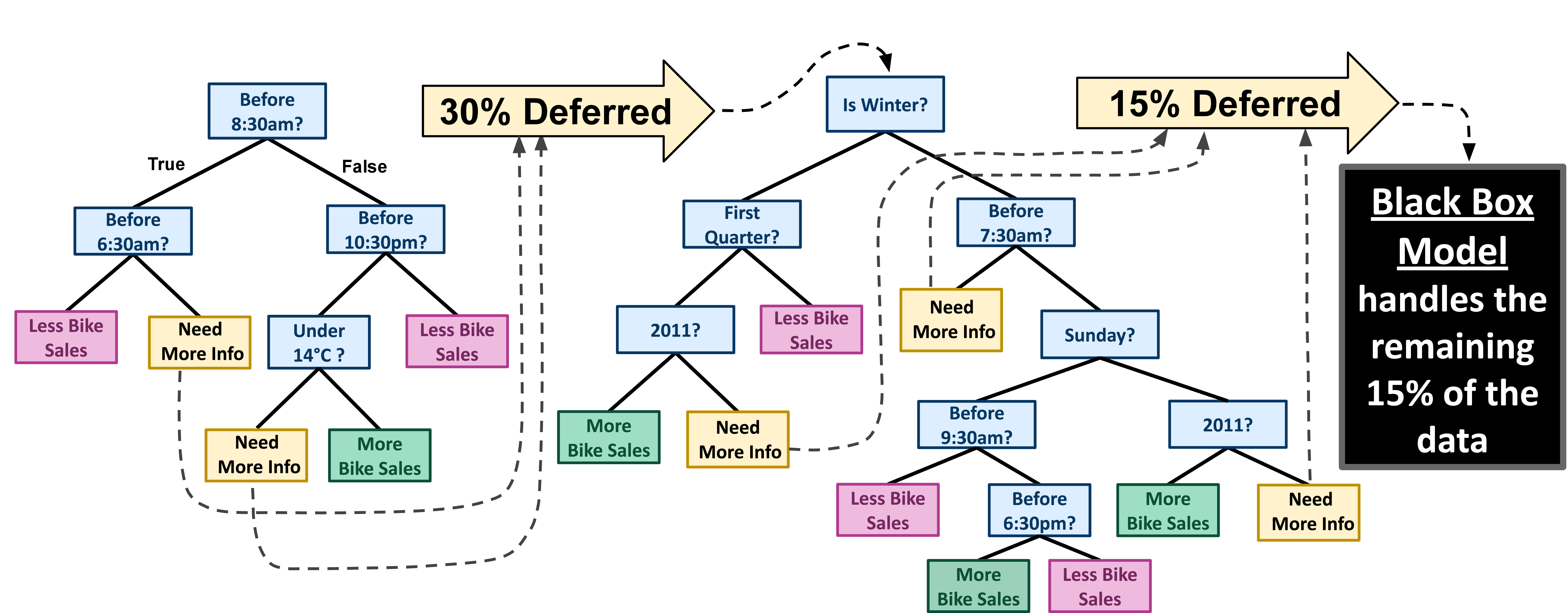
We present a tree-based hybrid-interpretable model that minimizes deferral rate while matching the performance of more complex ensembles. To learn this model, we iteratively focus on subsets of the data where simple models provably cannot perform as well as a black box model. This leads to a new model class, Multistage Defer Trees (MDTs), where each tree can either make a prediction or defer to the next stage; the final stage may then defer some samples to a black box model if required.
To train MDTs, we introduce an alternating optimization procedure in which the deferred-to model evolves with each stage of the MDT. As this process unfolds, the set of deferred points decreases monotonically, and the later stages and fallback model become increasingly specialized to those points. This allows the model to defer only on a small fraction of inputs while maintaining high accuracy. When the fallback is a sparse model (i.e., a single decision tree or EBM [10]), even these deferral cases remain interpretable; when the fallback is a black box, performance can be matched with minimal reliance on that model. Crucially, because deferred points are confined to a tightly constrained region of the feature space, the fallback model can be compressed, producing simpler but equivalent representations of even complex ensembles.
Our contributions are as follows.
We introduce Multistage Defer Trees (MDTs), a new model class that allocates complexity adaptively, based on the difficulty of different regions of the feature space.
We develop an iterative algorithm for training MDTs that successively narrows the deferral region, while borrowing strength from surrounding regions, to learn specialized trees that generalize well.
We provide algorithms to compress MDTs into sparse single-tree or rule-list representations and extend this framework to compress the fallback model when it is a tree or tree ensemble.
We demonstrate improved accuracy–deferral–sparsity trade-offs where such trade-offs exist.
2 Related Work↩︎
2.0.0.1 Hybrid Approaches
[5] introduces hybrid models for interpretability: an interpretable rule set or linear model makes predictions on some of the data, while deferring to fixed black box predictions on the remaining data. This allows users to navigate a tradeoff between the model accuracy and the amount of samples using interpretable model predictions. This framework, in turn, connects to work in deferral models [11], [12], rejection learning [13], [14], selective classification [15], and abstention-based learning [16], [17]. Hybrid models have primarily been applied to simple rule set models or linear models [4]–[8]. One recent work explores a gradient-based method to learn a complex (100-1000 leaves) decision tree, which defers to a black box based on computing the proximity to the decision boundary [9]; by contrast, our work learns a sparser sequence of trees that directly defer where the black box is most helpful, and iteratively reduces this deferral region.
2.0.0.2 Decision Tree Optimization
Decision trees are classically optimized with highly scalable greedy algorithms [18], [19]. Such algorithms can be ideal for popular ensembles of many trees [20], [21]. More recent work, however, has revisited the use of less scalable, higher quality individual tree algorithms, to reduce the need for this level of model complexity and to allow use of a single well-performing sparse tree classifier for domains where interpretability is needed. In recent years, global optimization of individual trees has become reasonably tractable for bounded depth and sparsity [22]–[29]. This problem is nevertheless NP-hard and does struggle to scale to cases with many features. Recent work sacrifices global optimality in exchange for improved scalability and runtime while maintaining performance close to optimal [30]–[32]. Other approaches add anytime behavior, allowing early termination with high-quality solutions [33]–[35].
We fit a small sequence of trees that nearly matches the performance of a significantly more complex ensemble. Because MDTs rely on only a few sparse trees, we can afford to optimize each component tree more carefully than in standard greedy tree induction while still requiring the overall procedure to scale. Given this need for both higher-quality component trees and scalability, we use a version of the polynomial-time LicketySPLIT algorithm from [30], which we modify to support sample weights and deferral; our theory provides guarantees achievable when each component tree is exactly optimal with respect to misclassification error, deferral rate, and tree complexity. Many near-optimal decision tree algorithms, including LicketySPLIT, operate on binarized features, which are often constructed using ThresholdGuessing [36]; we use the same binarization method.
2.0.0.3 Compressing Tree Ensembles
[37] present an algorithm to find the sparsest single decision tree with identical 0-1 predictive behaviour to a given tree-based ensemble (though not necessarily identical predicted probabilities). They additionally provide practical relaxations to allow for faster computation (removing the certificate that the tree is the sparsest equivalent form) or sparser representations (providing extra pruning in areas with no support in the training data). [38] translate an XGBoost tree ensemble [21] to a single tree, with some approximation loss. [36] take a slightly different approach to learn a single tree when provided with a tree-based ensemble, using the ensemble’s predictions to provide heuristic pruning of the search space for an otherwise globally optimal tree. All three methods afford more interpretable single tree alternatives when provided with an ensemble model, though to guarantee matching performance with that ensemble, these approaches often find trees with many more leaves than is ideal for interpretability.
In the hybrid component of our own algorithm, we incorporate information from a black box model in a fundamentally different way than the above approaches. Our goal is not to match the black box model’s predictions exactly, nor to accelerate an optimal tree search; instead our goal is to use the black box to resolve subspaces of the data for which interpretable algorithms cannot find an accurate simple model; this allows us to find models that are transparent on much of the data, without sacrificing meaningful accuracy relative to the black box. While we discuss several useful properties when the black box is a tree-based ensemble, our approach inherits the more general-purpose properties of hybrid models and can work with any black box model, since all we need for training is to retrain the model and obtain its prediction vector on the dataset.
Once we have identified the set of points for which we defer to a black box, if our black box is a tree ensemble it is possible to apply any of these compression methods, focusing on the subset of data for which our model defers (or even to apply approximate compression methods, such as the method proposed by [39]). This can further improve the interpretability of the tree, while simplifying the scope of the task to only those subspaces for which we know we need to use compression rather than learning a simple model.
3 Methodology↩︎
3.0.0.1 Notation.
Let \(\mathcal{X} \subseteq \mathbb{R}^p\) denote an input space with \(p\) features and let \(\mathcal{Y}=\{0,1\}\) denote the label space. Training data is denoted as \(\mathcal{D} = \{(x_i,y_i)\}_{i=1}^N \subseteq \mathcal{X} \times \mathcal{Y}\). When this data is weighted, we denote the dataset as \(\mathcal{D}^w\) for weight vector \(w \in \mathbb{R}_{\ge 0}^N\). We write \(\mathbb{1}\{\cdot\}\) for the indicator function. For a binary decision tree \(T\), let \(|T|\) denote its number of leaves, and let \(T(x)\) denote the label predicted by \(T\) for input \(x\).
A standard binary decision tree recursively partitions \(\mathcal{X}\) by internal boolean split nodes and assigns a prediction at each leaf. We generalize this object by allowing a leaf to output either a class label or a special defer action, indicating that prediction should be deferred to a subsequent model.
Definition 1 (Defer tree). A defer tree* \(T\) is a binary tree whose leaves are labeled by elements of \(\mathcal{Y} \cup \{\mathrm{defer}\}\). For some fallback model B, the prediction of a defer tree is: \[\hat{y}_{T,B}(x) = \begin{cases} T(x), & \text{if } T(x) \neq \mathrm{defer},\\[4pt] B(x), & \text{otherwise}. \end{cases}\]*
For a fixed fallback model \(B\), we can train a single defer tree \(T\) by optimizing the objective \(\mathcal{L}_{T, B}\) defined by \[\mathcal{L}_{T, B}(\mathcal{D}^w, \tau, \eta) = \tau\,(|T|-1) + \sum_{i=1}^N w_i\,(\mathbb{1}\{\hat{y}_{T,B}(x_i) \neq y_i\} + \eta \mathbb{1}\{{{T}(x_i) = \mathrm{defer}}\}),\] where the hyperparameter \(\tau\) penalizes the number of splits in the tree, \(\eta\) penalizes deferrals to a black box model \(B\), and \(w\) denotes the sample weights for dataset \(\mathcal{D}\). We optimize this objective using a modified version of LicketySPLIT [30]; details are given in Appendix 10.2.
A single defer tree can improve accuracy over a fully interpretable model by deferring difficult samples to a black box. However, those deferred samples are exactly where the original problem remains unresolved. On that subset, we are still relying on a black box, and we would like to recover interpretability there as well. It may seem natural to simply grow the tree further on that region, but if the original defer tree is already optimal, this is no longer possible. An optimal defer tree comes with a certificate that rules out further improvement: any attempt to replace a deferral with an interpretable prediction must increase the objective. In particular, matching the black box’s accuracy on the deferred subproblems would require a complexity increase whose leaf penalty outweighs the savings from eliminating deferral (formalized in Proposition 1 in the appendix).
To overcome this limitation, we move beyond a single tree and introduce a sequential model that allows further improvement on the deferred region of a single defer tree.
Definition 2 (Multistage defer tree). A multistage defer tree (MDT) of length \(K\) is an ordered sequence \[T_{1:k} = (T_1,\dots,T_K),\] where each \(T_i:\mathcal{X}\to \mathcal{Y}\cup\{\mathrm{defer}\}\) for \(i=1,\dots,K\) is a defer tree. For some fallback model \(B:\mathcal{X} \to \mathcal{Y}\), the prediction of the MDT is \[\hat{y}_{T_{1:k};B}(x) = \begin{cases} T_{1}(x), & \text{if } T_1(x) \neq \mathrm{defer},\\[4pt] \hat{y}_{T_{2:k}, B}(x), & \text{otherwise}. \end{cases}\]
An MDT routes each input through a sequence of defer trees, where each stage either predicts immediately or defers to the next stage. It also affords interpretability benefits relative to other tree-based ensembles. As discussed in [thm:rule-list] below, our multistage defer trees can be represented compactly as a rule list. This is significantly smaller than the rule list representations of other ensembles, such as random forests or boosted trees, where even the number of literals in a single antecedent can grow with the sum of depths across all trees (see 2 in the appendix).
theoremrulelistmdt An MDT with \(K\) stages admits a rule-list representation, in which each non-deferral leaf in any stage contributes exactly one antecedent. Consequently, if stage \(j\) has \(n_j\) non-deferral leaves, the total number of antecedents is \(\sum_{j=1}^K n_j\).
Because of Theorem [thm:rule-list], we can define a simple objective for MDTs that corresponds to an upper bound on the rule list deferral objective in [7] applied to the rule list form of the MDT (we discuss our relation to existing objectives in Appendix 11).
For a given MDT \((T_1, \ldots, T_k)\) and fallback model \(B\), let its objective \(\mathcal{L}_{T_{1:k}, B}\) be: \[\mathcal{L}_{T_{1:k}, B}(\mathcal{D}^w, \tau, \eta) = \tau \sum_{j=1}^k \bigl(|T_j|-1\bigr) + \sum_{i=1}^N w_i\,(\mathbb{1}\{\hat{y}_{T_{1:k,B}(x_i) \neq y_i}\} + \eta \mathbb{1}\{{{T_{1:k}}(x_i) = \mathrm{defer}}\}),\]
where \({T}_{1:k}(x)\) denotes the output of the sequence of trees \((T_1,\dots,T_k)\).
3.1 Training Multistage Defer Trees↩︎
When optimizing our MDT objective \(\mathcal{L}_{T_{1:k}, B}\), we can expand the structure from the top down, training a defer tree at each stage on the remaining deferred region with our single defer tree objective \(\mathcal{L}_{T,B}\). When we do so, Proposition [prop:monotone-topdown] shows that we monotonically decrease the objective defined above.
propositiontopdownimprovement Consider an iterative procedure where we train a single defer tree on the samples that have not been in previous stages. Define weights for stage \(j\) that zero out all samples that are not deferred by that stage: \[w^{(j)}_i := w_i^{(j-1)}\mathbb{1}\{T_{j-1}(x_i)=\mathrm{defer}\}, \quad w^{(1)}_i := w_i.\]
Let \(\Delta_j\) be how much we improve on the objective of the deferred dataset \(\mathcal{D}^{w^{(j)}}\) with defer tree \(T_j\), relative to deferring to a black box \(B\):
\[\Delta_j = L_{\mathrm{defer}, B}(\mathcal{D}^{w^{(j)}}, \tau, \eta) - L_{T_j, B}(\mathcal{D}^{w^{(j)}}, \tau, \eta).\]
With this iterative procedure, the total improvement of the model relative to the black box is the sum of improvements of each single defer tree relative to deferral. \[\mathcal{L}_{T_{1:k}, B}(\mathcal{D}^w, \tau, \eta) = L_{\mathrm{defer}, B}(\mathcal{D}^{w^{}}, \tau, \eta) - \sum_{j=1}^k \Delta_j.\]
While Proposition [prop:monotone-topdown] motivates our approach, there is a risk of a hybrid model deferring to the black box primarily in regions where the black box has overfit. Consider subregions of the space where a black box’s performance is especially high due to sample bias. These are also regions where it will be difficult for a simple model to match that performance, so a hybrid model is likely to defer in this case, leading to high test error in deferral cases.
Even for a single defer tree, the black-box component generalization can be a substantial issue. Table 2 in the appendix shows that the test error of a black box in the deferred region can be more than an order of magnitude higher than the test error of the simple model in the non-deferred region. To address this, we also need to leverage the rest of the data to improve generalization.
We can continue to refine an MDT without inducing overfitting by reweighting the training distribution: non-deferred points are downweighted based on their distance to the deferred region, rather than assigning them no weight. At a high level, we will accomplish this via an alternating optimization procedure that iteratively 1) trains both a black box and a defer tree on a dataset and 2) trains a black box and a defer tree on a weighted dataset that places more importance on deferred points.
Let \(\mathcal{D}_{k-1} \subseteq \mathcal{X}\) denote the set of deferred points after stage \(k-1\). For any sample \(x_i \not \in \mathcal{D}_{k-1}\), let \(\textrm{defer\_dist}_{T_{1:k-1}}(x_i)\) denote the \(\ell_1\)-norm (taken in quantile space, more information in Appendix 9) of the minimal change to \(x_i\) such that it would be deferred by \(T_{\textrm{1:k-1}}\). Using this distance, we define training weights \(w_i\) for the next iteration (on the first iteration, all weights are 1). \[w_i \;=\; \begin{cases} 1, & \text{if } x_i \in \mathcal{D}_{k-1} \\[6pt] (1 - \mu)\,(1 +\textrm{defer\_dist}_{T_\textrm{{1:k-1}}}(x_i))^{-\gamma}, & \text{if } x_i \notin \mathcal{D}_{k-1}. \end{cases}\] Here, \(\mu \in [0,1]\) controls how much we uniformly scale down the weights of the non-deferred region, while \(\gamma \geq 0\) controls how strongly the weights decay with distance from the deferred region. When \(\gamma=0\), this reduces to assigning weight \(1-\mu\) to each non-deferred point. \(\mu=1\) places weight solely on the deferred points.
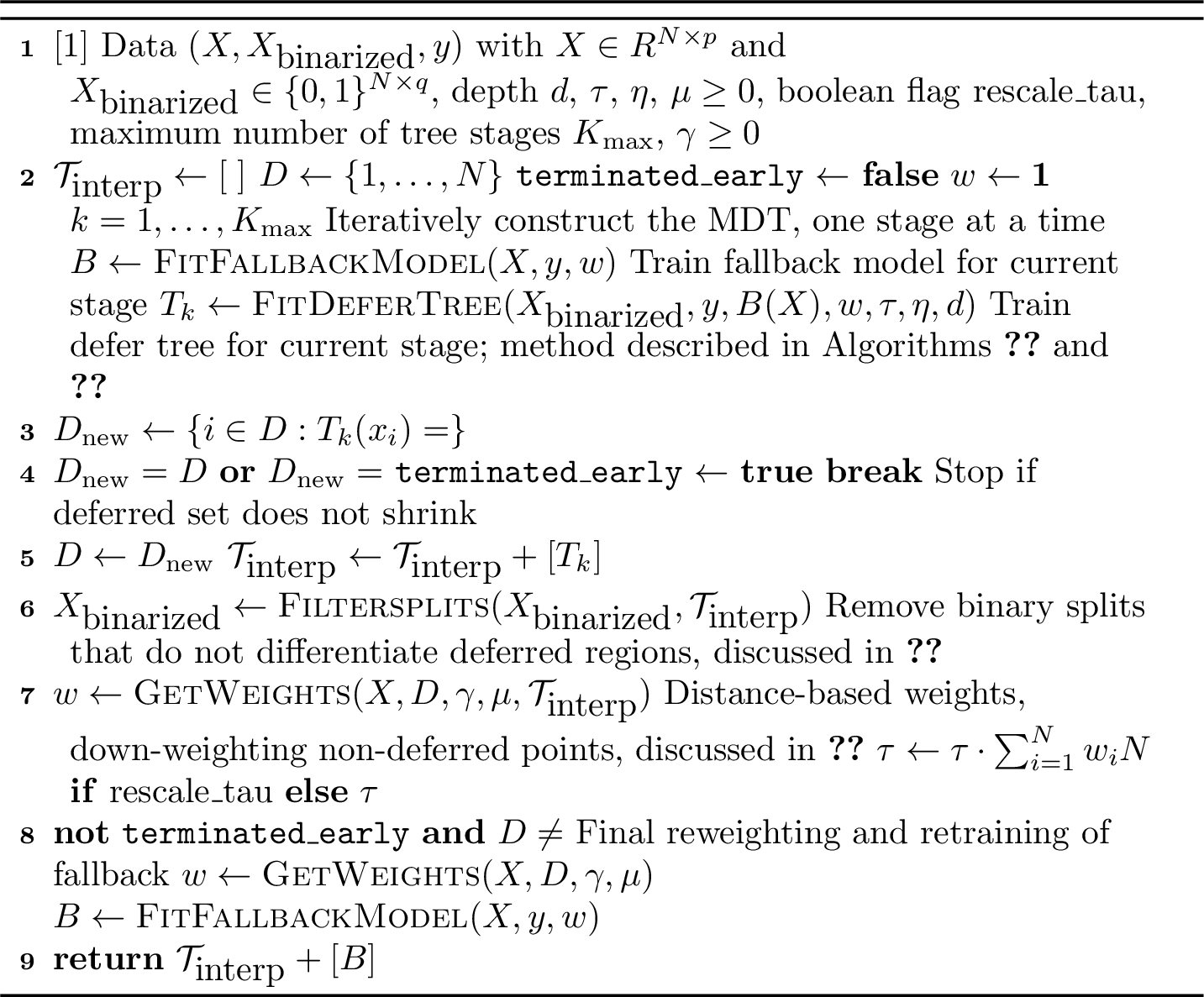
Algorithm 2 describes our approach to allow the fallback model and the next defer tree to iteratively update together. At each stage, we fit a fallback model \(B\) and a defer tree on the full dataset using the current weights (lines 7-9), where the weights are all 1 for the first pass (line 4). We then update core information for future iterations. We then update the active deferred set \(D\) to the subset of points that are still deferred (lines 10-15). If we decreased the size of the deferred set, we then add the tree to the sequence (line 16) and move to the next stage. To prepare for the next stage, we first filter out any splits that are provably irrelevant to our remaining deferral region (line 17). We then compute weights based on distances to the feasible deferred region (line 19), and optionally update the leaf penalty \(\tau\) (line 21).
The procedure terminates when \(D\) becomes empty or stops decreasing in size (lines 10-15). If the loop reaches \(K_{\max}\) without early termination and \(D\) is still nonempty (an iteration limit), we perform one final update of the fallback model using the latest weights (lines 23-27), since the previous fallback model was trained on the previous set of weights. In Appendix 10, we also describe early stopping criteria based on model complexity (e.g., per-stage size, equivalent rule list size, or equivalent single-tree size), along with efficient online updates to enforce these constraints.
For brevity, we defer additional theoretical results to Appendix 6. For instance, we show that the distance-based weights arise as a Gibbs distribution minimizing an entropy-regularized objective.
3.2 Feasible Region Tracking↩︎
Algorithm 2 specifies the high-level training procedure, but efficiently implementing lines 10, 12, and 25 requires viewing the deferral region geometrically as a union of axis-aligned hyperrectangles.
Let \(\Lambda_k^{\text{defer}}\) denote the set of defer leaves of tree \(k\). Each defer leaf \(\lambda \in \Lambda_k^{\text{defer}}\) corresponds to an axis-aligned hyperrectangle in feature space (a defer subregion), denoted \(R(\lambda)\). The total deferral region after stage \(k\) can be written as a set of defer subregions in the following way:
\[\mathcal{S}_k := \left( \left\{ \bigcap_{t=1}^k R(\lambda_t) \;\middle|\; (\lambda_1,\dots,\lambda_k)\in \Lambda_1^{\mathrm{defer}}\times\cdots\times\Lambda_k^{\mathrm{defer}} \right\} \right) \setminus \{\emptyset\}.\]
We refer to each element \(\bigcap_{t=1}^k R(\lambda_t)\) in the set \(\mathcal{S}_{k}\) as a defer subregion. Each such subregion remains an axis-aligned hyperrectangle, since intersections of axis-aligned hyperrectangles preserve this structure. Many such subregions may be empty (infeasible), e.g., \(age \leq 20\) in one stage and \(age > 25\) in another; we detect and discard these cases.
Because our iterative procedure refines only the set of subregions that defer, we can update this set iteratively. Suppose \(\mathcal{S}_{k-1}\) is the set of defer subregions for \(T_1 \cdots T_{k-1}\); then we can update it to be the set of defer subregions for \(T_1 \cdots T_{k}\) via pairwise intersections between the existing defer subregions and the defer subregions of \(T_{k}\):
\[S_k \leftarrow \left\{ \, s \cap R(\lambda_k) \;\middle|\; s \in S_{k-1},\;\lambda_k \in \Lambda_k^{\mathrm{defer}} \right\} \setminus \{\emptyset\}.\]
Once we have \(\mathcal{S}_k\), we can iterate over its elements to compute the distance from each point to each deferred subregion, and use the minimum such distance to measure how far the point is from being deferred. Likewise, for each column \(j\) of \(X_{\text{binarized}}\), we can discard it if its value is fixed across all feasible subregions; that is, the corresponding binarized predicate has the same truth value for every possible point in every subregion in \(\mathcal{S}_k\). Concretely, we map column \(j\) to its corresponding split \((f \le \nu)\) via its metadata, and discard it if either \(\forall s \in \mathcal{S}_k,\;\mathrm{\small ImpliesTrue}(s,f,\nu)\) or \(\forall s \in \mathcal{S}_k,\;\mathrm{\small ImpliesFalse}(s,f,\nu)\) (methods provided in 8). Appendix 10 presents a version of Algorithm 2 with these changes to improve efficiency.
Feasible region tracking can also be used to compress the resulting MDT. In Appendix 8, we provide an algorithm to compress the MDT into a single defer tree. We recursively expand each defer leaf by substituting the next-stage tree, while tracking the corresponding subregion of the feature space that we are in. If a split is guaranteed to evaluate the same way throughout this region (i.e., always True or always False), we can replace the node with the corresponding child. We also provide algorithms to further simplify the MDT when redundant splits remain; this has the effect of shortening the rules used in a MDT’s rule-list representation. We can apply either of these techniques to each tree in a tree ensemble, using the set of subregions in which that tree may be evaluated.
4 Experiments↩︎
We compare our MDTs and the defer tree method to state-of-the-art tree ensembles (XGBoost [21], Random Forest [20]), sparse additive tree models (FIGS [40]), and existing hybrid interpretable baselines (HyRS [4], [5], Pre- and Post- CORELS [7]) on a wide range of datasets. We also implemented the hybrid interpretable model from [8], and refer to the method as FLMM. Lastly, we add a logistic regression baseline, which defers when the estimated probability is close to 0.5. Our key questions are as follows. (1) Can MDTs provide black-box comparable accuracy for a small deferral rate? (2) How do MDT deferral rates and accuracy compare to existing deferral methods? (3) How complex are state-of-the-art MDTs?
| Dataset | Non-Deferral Tree | FIGS | Random Forest | MDT+XGB \(\le\)25% (Ours) | XGBoost |
|---|---|---|---|---|---|
| Abalone | \(0.6314 \pm 0.0060\) | \(\mathbf{0.6381 \pm 0.0030}\) | \(0.6314 \pm 0.0035\) | \(\underline{0.6333 \pm 0.0069}\) | \(\underline{0.6323 \pm 0.0070}\) |
| Adult | \(0.8598 \pm 0.0017\) | \(0.8589 \pm 0.0021\) | \(0.8619 \pm 0.0017\) | \(0.8667 \pm 0.0021\) | \(\mathbf{0.8701 \pm 0.0013}\) |
| Aging | \(\mathbf{0.8028 \pm 0.0034}\) | \(0.7944 \pm 0.0047\) | \(\underline{0.8014 \pm 0.0036}\) | \(\mathbf{0.8028 \pm 0.0034}\) | \(\underline{0.8000 \pm 0.0028}\) |
| Bank | \(0.9051 \pm 0.0008\) | \(0.9052 \pm 0.0017\) | \(0.9069 \pm 0.0008\) | \(\underline{0.9087 \pm 0.0008}\) | \(\mathbf{0.9090 \pm 0.0007}\) |
| Bike | \(0.9346 \pm 0.0021\) | \(0.9113 \pm 0.0039\) | \(0.9426 \pm 0.0017\) | \(\underline{0.9486 \pm 0.0024}\) | \(\mathbf{0.9500 \pm 0.0023}\) |
| California | \(0.8893 \pm 0.0024\) | \(0.8774 \pm 0.0015\) | \(0.9019 \pm 0.0032\) | \(\underline{0.9099 \pm 0.0020}\) | \(\mathbf{0.9101 \pm 0.0022}\) |
| Churn | \(0.9424 \pm 0.0036\) | \(0.9434 \pm 0.0057\) | \(0.9506 \pm 0.0032\) | \(\underline{0.9566 \pm 0.0028}\) | \(\mathbf{0.9574 \pm 0.0028}\) |
| Droid | \(0.9627 \pm 0.0011\) | \(0.9601 \pm 0.0005\) | \(\underline{0.9715 \pm 0.0006}\) | \(0.9709 \pm 0.0005\) | \(\mathbf{0.9718 \pm 0.0004}\) |
| Heloc | \(\underline{0.7052 \pm 0.0107}\) | \(0.6840 \pm 0.0074\) | \(\underline{0.7080 \pm 0.0102}\) | \(\underline{0.7056 \pm 0.0107}\) | \(\mathbf{0.7116 \pm 0.0108}\) |
| Jasmine | \(0.8037 \pm 0.0077\) | \(0.7983 \pm 0.0054\) | \(\mathbf{0.8218 \pm 0.0085}\) | \(\underline{0.8161 \pm 0.0100}\) | \(\underline{0.8214 \pm 0.0071}\) |
| Phishing | \(0.9528 \pm 0.0017\) | \(0.9392 \pm 0.0019\) | \(\underline{0.9721 \pm 0.0013}\) | \(\underline{0.9728 \pm 0.0017}\) | \(\mathbf{0.9733 \pm 0.0015}\) |
| Pol | \(0.9723 \pm 0.0012\) | \(0.9631 \pm 0.0018\) | \(0.9823 \pm 0.0007\) | \(\mathbf{0.9849 \pm 0.0003}\) | \(\underline{0.9845 \pm 0.0007}\) |
| Rl | \(0.7614 \pm 0.0052\) | \(0.7163 \pm 0.0094\) | \(0.8074 \pm 0.0058\) | \(0.7968 \pm 0.0089\) | \(\mathbf{0.8278 \pm 0.0034}\) |
| Shopping | \(0.9010 \pm 0.0025\) | \(0.8988 \pm 0.0021\) | \(\underline{0.9046 \pm 0.0012}\) | \(\underline{0.9047 \pm 0.0016}\) | \(\mathbf{0.9057 \pm 0.0015}\) |
| Spambase | \(0.9254 \pm 0.0016\) | \(0.9222 \pm 0.0034\) | \(\underline{0.9517 \pm 0.0014}\) | \(\underline{0.9500 \pm 0.0024}\) | \(\mathbf{0.9528 \pm 0.0023}\) |
| Wine | \(0.8340 \pm 0.0015\) | \(0.8391 \pm 0.0039\) | \(\underline{0.8848 \pm 0.0042}\) | \(0.8788 \pm 0.0052\) | \(\mathbf{0.8864 \pm 0.0022}\) |
4pt
To answer these questions, we need to determine the best configurations for hybrid interpretable models subject to a particular constraint on test deferral rate. To do so, we adopt a semi-supervised approach: for each train/test split and maximum deferral rate \(c\), we choose the hyperparameter that maximizes the average validation accuracy, while deferring on at most \(c\) proportion of the test set. Note that deferral is independent of labels, so this is fully semi-supervised.
In Appendix 13 (Tables 6 and 3), we show that the gap between train and test deferral rates is always small, suggesting that a fully supervised selection procedure would yield nearly identical results. Indeed, we show this is the case in the appendix (28). Additional information on our experiment setup is in Appendix 12; all results are averaged across five train/test splits.
To answer question (1), Table 1 reports test accuracy across datasets. MDT+XGB (with at most 25% deferral) is consistently competitive even with the strongest black box baselines: it is frequently closer to state-of-the-art performance than random forests and almost always within the 95% confidence interval of the best method. Furthermore, it outperforms the sparse ensemble model FIGS on nearly all datasets. MDT also outperforms a single tree, non-deferral ablation, demonstrating that the multistage training and deferral is core to MDT’s success.

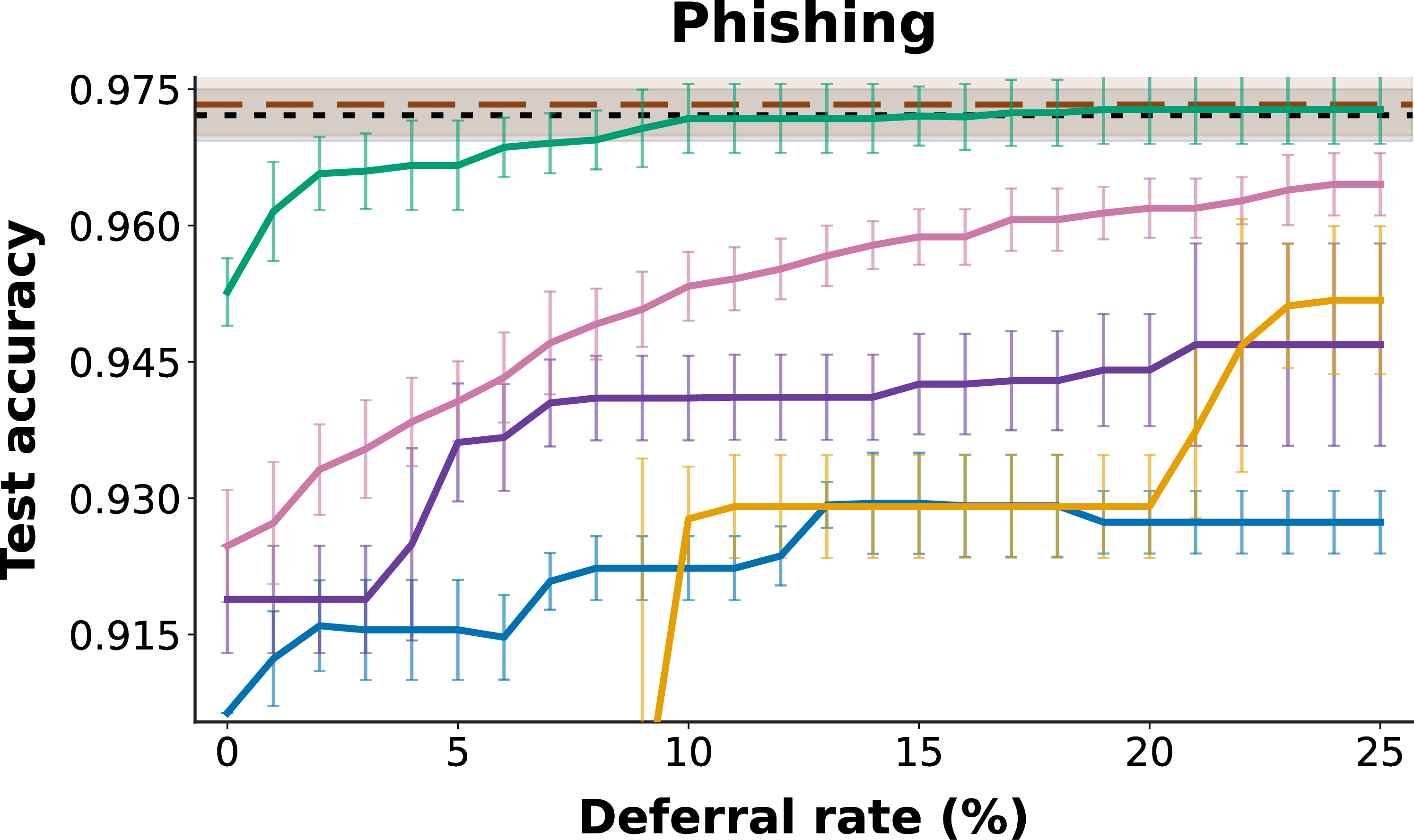

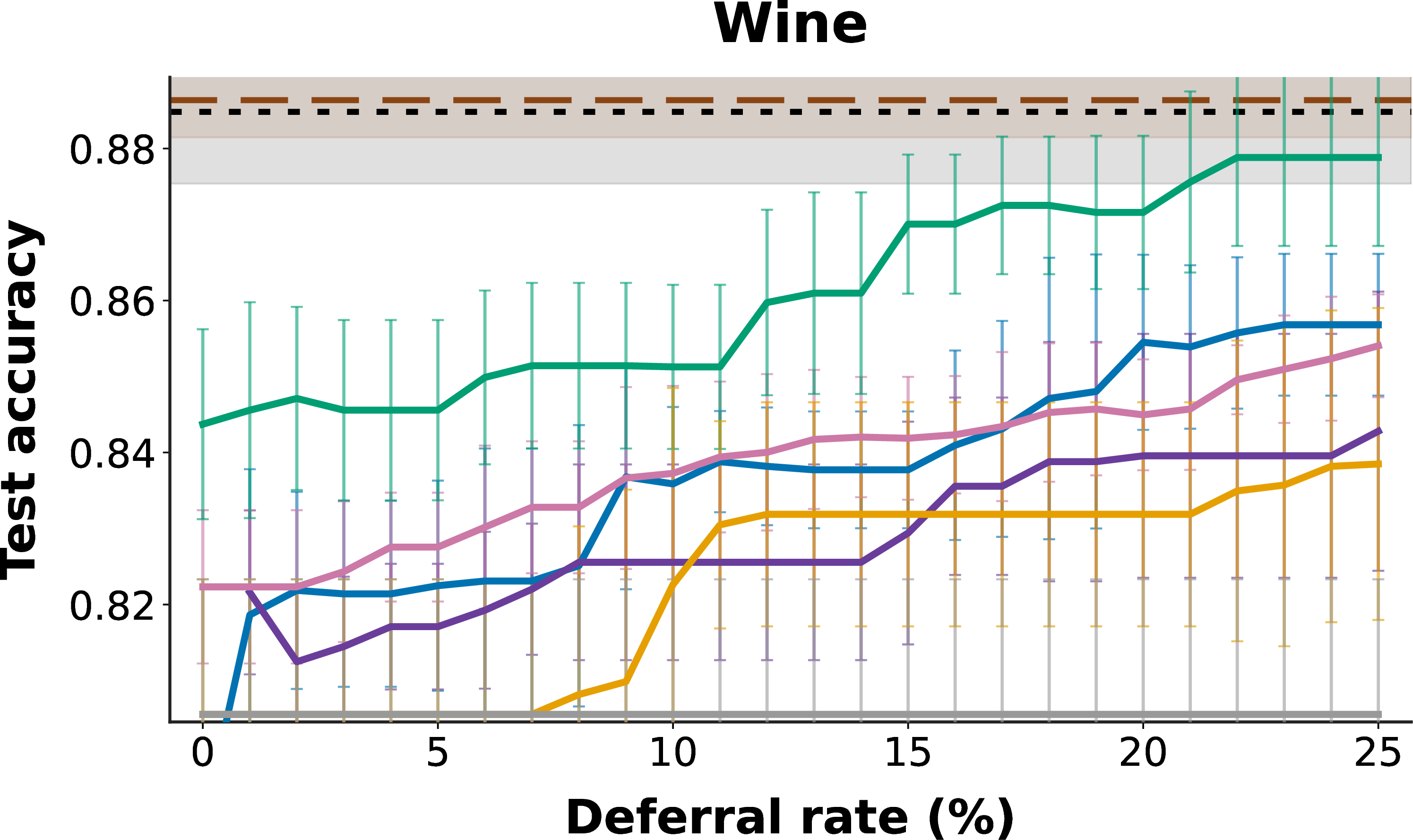

Figure 3: Test accuracy (mean \(\pm\) standard deviation) as a function of deferral rate across datasets..

Figure 4: CDF of deferral thresholds required to have accuracy within \(2.0\%\) of XGBoost. Each curve shows the fraction of datasets for which a method achieves this accuracy within a given deferral rate..
To answer question (2), we compare MDTs to other hybrid-interpretable models in Figures 3 and 4. In Figure 3, we compare hybrid-interpretable models on datasets where the accuracy-interpretability tradeoff is high (a single tree is \(> 2 \%\) less accurate than a black box).
On all four datasets, MDT+XGB consistently outperforms all other baselines. On California, MDT+XGB matches the mean accuracy of XGBoost at 25% deferral, a level that no competing method achieves within the same deferral budget. Figure 4 shows the deferral rate required to achieve accuracy within \(2.0\%\) of XGBoost across all 24 datasets (the full list of datasets is in Appendix 12). At around \(40\%\) deferral, our MDT+XGB method can come within this amount of XGBoost for all datasets. No existing method can match this without deferring the majority of the time.
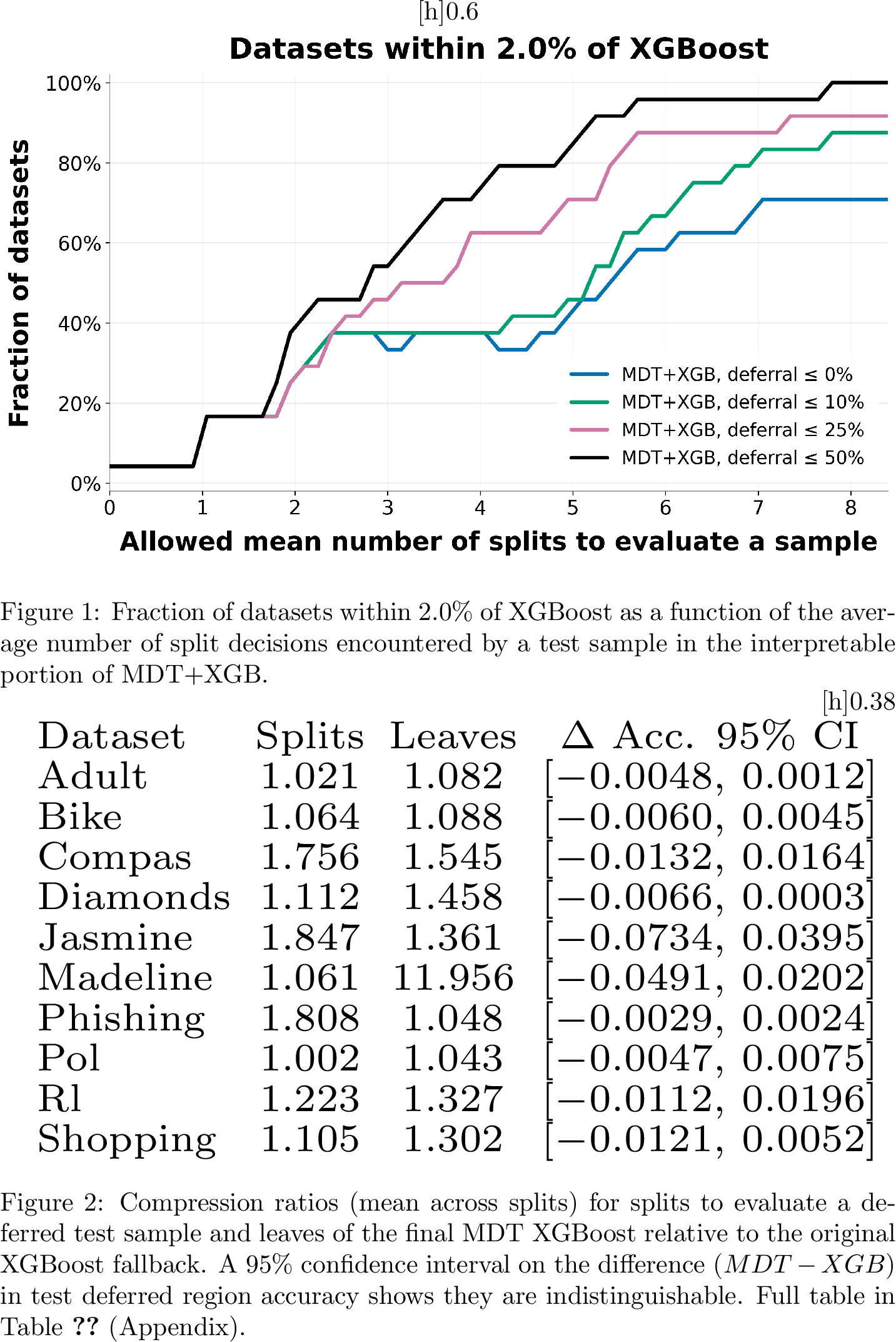
To answer question (3), Figure [fig:sparsity95cdf95eps0025] shows the fraction of datasets that achieve accuracy within \(2.0\%\) of XGBoost as a function of the average number of split decisions encountered by a test sample while passing through the interpretable portion of the MDT. This average path-length constraint is enforced analogously to the deferral constraint. At 50% deferral, no dataset requires more than an average of 7.5 split decisions per sample to reach near-XGBoost performance, and the vast majority reach this threshold with at most an average of 5.5 split decisions per sample. Since MDTs only need to use a black-box component for a small proportion of samples, the black-box representations they learn are naturally more compressed. Figure [fig:dist95sparsity95sub] compares the distribution of the number of splits needed to evaluate samples that are deferred, either by (a) using the final fallback XGBoost model or (b) using the best XGBoost model for the whole dataset. Both (a) and (b) are trained with the same hyperparameter configuration, but approach (a) is trained using a weighting that emphasizes deferred points. The number of splits required to classify a sample is greatly reduced.
5 Conclusion↩︎
We introduce Multistage Defer Trees, a model class that adaptively allocates complexity by routing inputs through a sequence of sparse decision trees before deferring to a black-box model. Our training procedure progressively refines the defer region, combining distance-based weighting, which allows the model to borrow strength from nearby points, with compression techniques that track and simplify defer subregions. MDTs demonstrate that accuracy and interpretability need not be traded off globally, substantially improving the accuracy-deferral frontier. Future work could explore using multiple fallback models, possibly from different model classes.
Appendix Contents↩︎
=.apc
6 Proofs↩︎
Proof. For each stage \(j\), define the set of samples that reach stage \(j\) as \[D_j := \{i : T_1(x_i)=\cdots=T_{j-1}(x_i)=\mathrm{defer}\},\] with \(D_1=\{1,\ldots,N\}\).
Making the weight update \[w_i^{(j)} = w_i \mathbb{1}\{i \in D_j\}.\]
The all-defer baseline has decision tree objective \[L_{\mathrm{defer},B}(\mathcal{D}^w,\tau,\eta) = \sum_{i=1}^N w_i\Bigl( \mathbb{1}\{B(x_i)\neq y_i\}+\eta \Bigr),\]
Now consider the contribution of a single stage \(j\) on the samples that reach it. On the weighted dataset \(\mathcal{D}^{w^{(j)}}\), the single-tree defer objective is \[L_{T_j,B}(\mathcal{D}^{w^{(j)}},\tau,\eta) = \tau (|T_j|-1) + \sum_{i=1}^N w_i^{(j)} \Bigl( \mathbb{1}\{\hat{y}_{T_j,B}(x_i)\neq y_i\} + \eta \mathbb{1}\{T_j(x_i)=\mathrm{defer}\} \Bigr).\] The all-defer tree (a single defer leaf) on the same weighted dataset has objective \[L_{\mathrm{defer},B}(\mathcal{D}^{w^{(j)}},\tau,\eta) = \sum_{i=1}^N w_i^{(j)} \Bigl( \mathbb{1}\{B(x_i)\neq y_i\}+\eta \Bigr).\] Therefore, \[\Delta_j = L_{\mathrm{defer},B}(\mathcal{D}^{w^{(j)}},\tau,\eta) - L_{T_j,B}(\mathcal{D}^{w^{(j)}},\tau,\eta)\] equals \[-\tau(|T_j|-1) + \sum_{i=1}^N w_i^{(j)} \Bigl[ \mathbb{1}\{B(x_i)\neq y_i\}+\eta - \mathbb{1}\{\hat{y}_{T_j,B}(x_i)\neq y_i\} - \eta\mathbb{1}\{T_j(x_i)=\mathrm{defer}\} \Bigr].\]
Now sum the expression for \(\Delta_j\) over \(j=1,\ldots,k\): \[\sum_{j=1}^k \Delta_j = -\tau\sum_{j=1}^k (|T_j|-1) + \sum_{j=1}^k \sum_{i=1}^N w_i^{(j)} \Bigl[ \mathbb{1}\{B(x_i)\neq y_i\}+\eta - \mathbb{1}\{\hat{y}_{T_j,B}(x_i)\neq y_i\} - \eta\mathbb{1}\{T_j(x_i)=\mathrm{defer}\} \Bigr].\]
Using \[w_i^{(j)} = w_i \mathbb{1}\{T_1(x_i)=\cdots=T_{j-1}(x_i)=\mathrm{defer}\},\] we can rewrite the double sum sample-by-sample: \[\sum_{j=1}^k \sum_{i=1}^N w_i^{(j)} \Bigl[ \mathbb{1}\{B(x_i)\neq y_i\}+\eta - \mathbb{1}\{\hat{y}_{T_j,B}(x_i)\neq y_i\} - \eta\mathbb{1}\{T_j(x_i)=\mathrm{defer}\} \Bigr]\] \[\begin{align} &= \sum_{i=1}^N w_i \sum_{j=1}^k \mathbb{1}\{T_1(x_i)=\cdots=T_{j-1}(x_i)=\mathrm{defer}\} \Bigl[ \mathbb{1}\{B(x_i)\neq y_i\}+\eta \\ & - \mathbb{1}\{\hat{y}_{T_j,B}(x_i)\neq y_i\} - \eta\mathbb{1}\{T_j(x_i)=\mathrm{defer}\} \Bigr]. \end{align}\]
Fix a sample \(i\). Let \(r_i\) be the first stage that predicts a label: \[r_i := \min\{j : T_j(x_i)\neq \mathrm{defer}\},\] if such a stage exists. If no such stage exists, set \(r_i=k+1\).
There are 3 cases: (1.1, 1.2, and 2.1).
Case 1.1: \(j < r_i \leq k\). Here, sample \(i\) reaches stage \(j\) but it still defers.
Therefore, \(T_j(x_i)=\mathrm{defer}\), so the prediction used in the loss of training the single defer tree is \(\hat{y}_{T_j,B}(x_i)=B(x_i)\). Also, \(\mathbb{1}\{T_j(x_i)=\mathrm{defer}\}=1\). So, the bracket becomes \[\mathbb{1}\{B(x_i)\neq y_i\}+\eta - \mathbb{1}\{B(x_i)\neq y_i\} - \eta = 0.\]
So every stage before the first predicting stage contributes nothing to the improvement in the objective for that sample. Intuitively, before \(r_i\), the model is still doing exactly what the all defer tree does: defers to \(B\) and pays the penalty.
Case 1.2: \(j=r_i\le k\). The tree predicts.
We know \(T_{r_i}(x_i)\neq \mathrm{defer}\) and \(\mathbb{1}\{T_{r_i}(x_i)=\mathrm{defer}\}=0\). This is the first stage for which we make a prediction for this sample, so \(\hat{y}_{T_{r_i},B}(x_i) = \hat{y}_{T_{1:k},B}(x_i)\).
Therefore, the bracket becomes
| $${B(x_i)y_i}+ |
|---|
| {{T{1:k},B}(x_i)y_i}.$$ |
Since the full MDT does not defer on this sample, we also know \(\mathbb{1}\{\hat{T}_{1:k}(x_i)=\mathrm{defer}\}=0.\)
Appending this zero term will become useful later in the proof.
| $${B(x_i)y_i}+ |
|---|
| ( |
| {{T{1:k},B}(x_i)y_i} |
| + |
| {_{1:k}(x_i)=} |
| ).$$ |
Case 2.1: \(r_i=k+1\). Here, the MDT defers to the black box. No stage predicts. The sample is deferred by every stage.
Writing the consequences of this formally: \[T_1(x_i)=T_2(x_i)=\cdots=T_k(x_i)=\mathrm{defer}.\]
For every \(j \leq k\)
\[\hat{y}_{T_j,B}(x_i)=B(x_i)\]
and
\[\mathbb{1}\{T_j(x_i)=\mathrm{defer}\}=1.\]
Therefore, every bracket is
| $${B(x_i)y_i}+ |
|---|
| {B(x_i)y_i} |
7 ↩︎
0.$$
Now, with the three cases solved, we can look back at the double sum.
\[\sum_{j=1}^k \sum_{i=1}^N w_i^{(j)} \Bigl[ \mathbb{1}\{B(x_i)\neq y_i\}+\eta - \mathbb{1}\{\hat{y}_{T_j,B}(x_i)\neq y_i\} - \eta\mathbb{1}\{T_j(x_i)=\mathrm{defer}\} \Bigr]\] \[\begin{align} &= \sum_{i=1}^N w_i \sum_{j=1}^k \mathbb{1}\{T_1(x_i)=\cdots=T_{j-1}(x_i)=\mathrm{defer}\} \Bigl[ \mathbb{1}\{B(x_i)\neq y_i\}+\eta \\ & - \mathbb{1}\{\hat{y}_{T_j,B}(x_i)\neq y_i\} - \eta\mathbb{1}\{T_j(x_i)=\mathrm{defer}\} \Bigr]. \end{align}\]
We now claim that \(S_i\) is the entire inner sum over stages \(j=1,\ldots,k\) for one sample \(i\):
\[S_i = \mathbb{1}\{B(x_i)\neq y_i\}+\eta - \Bigl( \mathbb{1}\{\hat{y}_{T_{1:k},B}(x_i)\neq y_i\} + \eta\mathbb{1}\{\hat{T}_{1:k}(x_i)=\mathrm{defer}\} \Bigr).\]
Recall we showed that at most one \(j\) is nonzero for a fixed sample \(i\). If \(r_i=k+1\), every stage defers, so all terms are zero. We appended the zero term in Case 1.2 to give us this expression. The other two cases were evaluated to 0. \(S_i\) is precisely the sum of all of them, which simplifies to just Case 1.2.
Continuing, the double sum is
\[= \sum_{i=1}^N w_i S_i,\]
\[= \sum_{i=1}^N w_i \Bigl[ \mathbb{1}\{B(x_i)\neq y_i\}+\eta - \mathbb{1}\{\hat{y}_{T_{1:k},B}(x_i)\neq y_i\} - \eta\mathbb{1}\{\hat{T}_{1:k}(x_i)=\mathrm{defer}\} \Bigr].\]
Now plug this back into the sum over improvements,
\[\sum_{j=1}^k \Delta_j = -\tau\sum_{j=1}^k (|T_j|-1) + \sum_{i=1}^N w_i S_i.\]
\[\sum_{j=1}^k \Delta_j = -\tau\sum_{j=1}^k (|T_j|-1) + \sum_{i=1}^N w_i \Bigl[ \mathbb{1}\{B(x_i)\neq y_i\}+\eta - \mathbb{1}\{\hat{y}_{T_{1:k},B}(x_i)\neq y_i\} - \eta\mathbb{1}\{\hat{T}_{1:k}(x_i)=\mathrm{defer}\} \Bigr].\]
Rearranging, \[\begin{align} \sum_{j=1}^k \Delta_j &= \left[ \sum_{i=1}^N w_i \bigl( \mathbb{1}\{B(x_i)\neq y_i\}+\eta \bigr) \right] \\ &\quad - \left[ \tau\sum_{j=1}^k (|T_j|-1) + \sum_{i=1}^N w_i \Bigl( \mathbb{1}\{\hat{y}_{T_{1:k},B}(x_i)\neq y_i\} + \eta\mathbb{1}\{\hat{T}_{1:k}(x_i)=\mathrm{defer}\} \Bigr) \right]. \end{align}\] The second bracket is exactly the MDT objective:
\[\mathcal{L}_{T_{1:k},B}(\mathcal{D}^w,\tau,\eta) = \tau\sum_{j=1}^k (|T_j|-1) + \sum_{i=1}^N w_i \Bigl( \mathbb{1}\{\hat{y}_{T_{1:k},B}(x_i)\neq y_i\} + \eta\mathbb{1}\{\hat{T}_{1:k}(x_i)=\mathrm{defer}\} \Bigr).\]
Likewise, the first term is the defer leaf objective.
\[L_{\mathrm{defer},B}(\mathcal{D}^w,\tau,\eta) = \sum_i w_i(\mathbb{1}\{B(x_i)\neq y_i\}+\eta).\]
These two facts establish what we wanted to show. ◻
Proposition 1 establishes the relationship between sparsity, accuracy, and deferral for sparse decision trees of unbounded depth. Consequently, the same claim holds when the model class is restricted to decision trees of any fixed bounded depth \(d\).
Proposition 1 (Accuracy-deferral trade-off). Let \(T^*\) be an optimal defer tree and let \(v\) be a defer leaf. Define \(S_v = \{i : x_i \text{ reaches } v\}\).
For any decision tree \(U\) used to replace \(v\), define \[\Delta(U) = \sum_{i \in S_v} \mathbb{1}\{U(x_i) \neq y_i\} - \sum_{i \in S_v} \mathbb{1}\{B(x_i) \neq y_i\}.\] Then \[\Delta(U) \;\ge\; \eta\,|S_v| \;-\; \tau \bigl(|U| - 1\bigr).\] Let \(U(x_i)\) In particular, if \(U(x_i)=B(x_i)\) for all \(i \in S_v\), then \[|U| \;\ge\; 1 + \frac{\eta\,|S_v|}{\tau}.\]
Proof. We first note that whenever an optimal defer tree places a defer leaf \(v\) at a subproblem, then this choice must be at least as good (in objective) as both replacing \(v\) with a majority prediction and replacing \(v\) with a subtree rooted at that subproblem, regardless of whether the subtree itself contains defer leaves.
The proof is an exchange argument from the optimality of \(T^*\).
The defer-tree objective when referencing a base model with predictions \(B(x_i)\) is:
\[L_{\mathrm{defer}}(T) = \tau \bigl(|T|-1\bigr) + \sum_{i=1}^N \ell_T(i),\]
where
\[\ell_T(i) = \mathbb{1}\{T(x_i)\in Y,\; T(x_i)\neq y_i\} + \mathbb{1}\{T(x_i)=\mathrm{defer},\; B(x_i)\neq y_i\} + \eta\,\mathbf{\mathbb{1}}\{T(x_i)=\mathrm{defer}\}.\]
Take any decision tree \(U\), and form a new defer tree \(T'\) by replacing the defer leaf \(v\) in \(T^*\) with \(U\).
Then, one leaf is removed, and \(|U|\) are added.
\[|T'| = |T^*| - 1 + |U|,\]
\[|T'| - |T^*| = |U| - 1.\]
For every \(i \notin S_v\), the prediction path is unchanged, so the loss is unchanged.
For every \(i \in S_v\), it had previously faced a penalty of \(\mathbb{1}\{B(x_i)\neq y_i\}+\eta\), because it was deferred. Now, it faces a cost of \(\mathbb{1}\{U(x_i)\neq y_i\}\).
Therefore,
\[L_{\mathrm{defer}}(T')-L_{\mathrm{defer}}(T^*) = \tau \bigl(|U|-1\bigr) + \sum_{i\in S_v}\mathbb{1}\{U(x_i)\neq y_i\} - \sum_{i\in S_v}\bigl(\mathbb{1}\{B(x_i)\neq y_i\}+\eta\bigr).\]
Because \(L_{\mathrm{defer}}(T')-L_{\mathrm{defer}}(T^*) \ge 0\), we get that
\[\Delta(U) \ge \eta |S_v| - \tau \bigl(|U|-1\bigr).\]
A corollary of this is if \(U(x_i)=B(x_i)\), for all \(i \in S_v\), then clearly
\[\sum_{i\in S_v}\mathbb{1}\{U(x_i)\neq y_i\} = \sum_{i\in S_v}\mathbb{1}\{B(x_i)\neq y_i\}.\]
Given that \(\Delta(U)=0\), we get \(0 \ge \eta |S_v| - \tau \bigl(|U|-1\bigr)\).
Equivalently,
\[|U| \ge 1+\frac{\eta |S_v|}{\tau}.\] ◻
Proof. We will use either \(|T_j|\) or \(\ell_j\) interchangeably to denote the number of leaves in stage \(j\), and \(d_j\) to denote the number of deferral leaves, not to be confused with the depth budget of each tree, which is \(d\).
In stage \(j\), each leaf corresponds to a unique root-to-leaf path, and hence to a conjunction of split conditions. For each non-deferral leaf \(\kappa\) in stage \(j\), let \(A_\kappa\) denote the conjunction of conditions along its path, and let \(y_\kappa \in \{0,1\}\) be its prediction.
We construct a rule list by concatenating \(K\) sections, one for each stage. In section \(j\), we include one antecedent (and the corresponding prediction) for each non-deferral leaf \(\kappa\) of stage \(j\): \[\text{if } A_\kappa \text{ then predict } y_\kappa.\]
Note that \(A_\kappa\), the conjunction of conditions along a root-to-leaf path in a single-stage tree, contains at most \(d\) conditions, since each tree has depth at most \(d\).
Because the leaves of a decision tree partition the input space, and each later stage operates only on the deferred region, the stages cover disjoint parts of the input space. Within a stage, there is no interaction between antecedents, so they may be listed in any order without ambiguity. While the choice of ordering may simplify individual antecedent conditions, it does not change the total number of rules.
We claim this rule list is equivalent to the MDT. Consider any input \(x\). In the MDT, \(x\) is first evaluated at stage \(1\). If it reaches a non-deferral leaf, the MDT outputs the corresponding prediction and halts. In the rule list, exactly the antecedent corresponding to that leaf is satisfied (and the consequent is the label of that leaf), so the first matching rule produces the same output.
If instead \(x\) reaches a deferral leaf at stage \(1\), then no antecedent from section \(1\) is satisfied, since that section contains only non-deferral leaves. The evaluation proceeds to section \(2\), mirroring the MDT’s transition to stage \(2\). Repeating this argument inductively, the antecedent that is satisfied corresponds exactly to the non-deferral leaf reached by \(x\) in the MDT, and outputs the same prediction.
Thus, the rule list is equivalent to the MDT.
Finally, in stage \(j\), there are \(\ell_j - d_j\) non-deferral leaves, each contributing exactly one antecedent. Summing over all stages yields the total number of antecedents: \[\sum_{j=1}^K (\ell_j - d_j).\] ◻
Corollary 1 (MDTs do not have wide rules). Let a rule list be defined over conjunctions of feature queries, where each satisfied rule must immediately output a leaf prediction. Then, for any MDT composed of \(m\) defer trees each of depth \(d\), every rule in the equivalent rule-list representation of the interpretable component has at most \(d\) literals.
Proof. This follows direction from the construction discussed in [thm:rule-list], which uses paths in each tree as rules, each of which must be of depth at most \(d\). ◻
Proposition 2 (Majority-vote ensembles have wide rules). Let a rule list be defined over any conjunction of feature queries in a dataset, such that the true branch must be classified immediately with a leaf. Then there exist binary decision trees \(T_1,\dots,T_m\), each of depth \(d\), such that the classifier defined by their majority vote cannot be represented by an equivalent rule list unless some rule queries \(\Omega(md)\) literals.
Proof. Let each tree compute an XOR over \(d\) binary features, and suppose that the feature sets used by different trees are disjoint. Assume that all feature value combinations are possible. For an XOR over \(d\) features, no subset of features can determine the tree’s predictions.
Now consider any rule in an equivalent rule list whose condition is satisfied by at least one input, and that assigns a label. Let us consider using that rule as the first rule. Since the rule must classify the affected points immediately, its conjunction must be sufficient to determine the majority-vote prediction for every completion of the unqueried features.
To force the majority vote, the rule must determine the outputs of at least \(\lceil m/2 \rceil\) trees (for the even case, we assume ties can be broken arbitrarily). Because the trees use disjoint feature sets, determining the output of each such XOR tree requires querying all \(d\) of its features. Hence, the rule must contain at least \[d\left(\left\lceil \frac{m}{2}\right\rceil\right) = \Omega(md)\] literals. ◻
As we show in the next theorem, the distance-based weighting rule admits an entropy-regularized variational interpretation. Among all distributions, the normalized weights best balance the expected distance to being deferred and the amount of deviation from uniform (according to \(\gamma\)).
Proposition 3 (Gibbs form of distance-based weights).
For each training data point \(i\), take \(c_i := \log(1 + D_i)\) and let \(u\) be the uniform distribution over the training data points.
The following objective (with \(\gamma>0)\) has a unique minimizer (over all distributions \(q\) on the training data points) given by \(q_i \propto (1+D_i)^{-\gamma}\).
\[\mathcal{J}(q) = \mathbb{E}_q[c_i] + \frac{1}{\gamma}\mathrm{KL}(q\|u)\]
Proof. Plugging in definitions,
\[\mathcal{J}(q)=\sum_{i=1}^N q_i c_i+\frac{1}{\gamma} \sum_{i=1}^N q_i \log\frac{q_i}{u_i}.\]
Because \(u_i=1/N\),
\[\log\frac{q_i}{u_i}=\log q_i-\log(1/N)=\log q_i+\log N.\]
This yields
\[\mathcal{J}(q)=\sum_{i=1}^N q_i c_i+\frac{1}{\gamma} \sum_{i=1}^N q_i \log q_i+\frac{1}{\gamma} \sum_{i=1}^N q_i \log N = \sum_{i=1}^N q_i c_i+\frac{1}{\gamma} \sum_{i=1}^N q_i \log q_i+\frac{1}{\gamma} \log N.\]
The third term is constant w.r.t \(q\), so we just need to optimize
\[\sum_{i=1}^N q_i c_i+\frac{1}{\gamma} \sum_{i=1}^N q_i \log q_i,\] subject to \(q\) being a probability distribution.
We form the Lagrangian:
\[L(q,\lambda)=\sum_{i=1}^N q_i c_i+\frac{1}{\gamma} \sum_{i=1}^N q_i \log q_i+\lambda\left(\sum_{i=1}^N q_i-1\right).\]
Because \(\frac{d}{dq_i}(q_i\log q_i)=\log q_i+1\), we get \[\frac{\partial L}{\partial q_i} = c_i+\frac{1}{\gamma}(\log q_i+1)+\lambda.\]
For an interior minimizer (assume no \(q_i = 0\)), this is 0.
\[c_i+\frac{1}{\gamma}(\log q_i+1)+\lambda=0.\]
Writing equivalent forms,
\[c_i+\frac{1}{\gamma}(\log q_i+1)+\lambda=0.\]
\[\log q_i = -\gamma c_i -1-\gamma\lambda.\]
\[q_i = \exp(-1-\gamma\lambda)\exp(-\gamma c_i).\]
Because \(\exp(-1-\gamma\lambda)\) does not depend on \(i\), we know \(q_i \propto e^{-\gamma c_i}=e^{-\gamma c_i}=e^{-\gamma \log(1+D_i)}=(1+D_i)^{-\gamma}.\)
Therefore, \[q_i \propto (1+D_i)^{-\gamma}.\]
Normalizing, as we know that \(q\) is a probability distribution,
\[q_i=\frac{(1+D_i)^{-\gamma}}{\sum_{j=1}^n (1+D_j)^{-\gamma}}.\]
We have found the only critical point in the interior (\(q_i > 0\)). We can show that it is both a minimizer and unique by strict convexity. We have the sum of a linear function (which is convex) and the negative entropy component is strictly convex (with \(0 \log 0 := 0\)). Since \(\gamma>0\), the sum is strictly convex. This suffices to show that the minimizer is unique and that it is an interior critical point. ◻
Proposition 4 (Size of the uncompressed single tree representation). Let an MDT chain be given by \[T_1 \to T_2 \to \cdots \to T_K \to W,\] where for each stage \(j\), \(T_j\) has \(\ell_j\) leaves, of which \(d_j\) are deferral leaves, and let \(W\) be a fallback model (such as a single-tree representation of a black box) with \(\ell_W\) leaves and no deferral leaves. Then the uncompressed single-tree representation of the chain has \[\sum_{j=1}^{K} \left(\prod_{i=1}^{j-1} d_i\right)(\ell_j-d_j) + \left(\prod_{i=1}^{K} d_i\right)\ell_W\] leaves.
Proof. A copy of \(T_j\) appears only when the input has been deferred through all earlier stages \(T_1,\dots,T_{j-1}\).
The tree \(T_1\) appears once. Each deferral leaf of \(T_1\) is replaced by a copy of \(T_2\), so there are \(d_1\) copies of \(T_2\). Each deferral leaf of each copy of \(T_2\) is replaced by a copy of \(T_3\), so there are \(d_1 d_2\) copies of \(T_3\).
Continuing inductively, the number of copies of \(T_j\) in the expanded tree is \[\prod_{i=1}^{j-1} d_i,\] with the convention that this product equals \(1\) when \(j=1\).
Each copy of \(T_j\) contributes \(\ell_j - d_j\) final (non-deferral) leaves, since its \(d_j\) deferral leaves are replaced by the root of the next stage. Therefore, the total number of final leaves contributed by all copies of \(T_j\) is \[\left(\prod_{i=1}^{j-1} d_i\right)(\ell_j - d_j).\]
Summing over all stages \(j=1,\dots,K\), the total number of final leaves contributed by the MDT stages is \[\sum_{j=1}^{K} \left(\prod_{i=1}^{j-1} d_i\right)(\ell_j - d_j).\]
If \(d_K \neq 0\), the remaining deferral leaves of stage \(K\) are replaced by copies of \(W\). The number of copies of \(T_K\) is \(\prod_{i=1}^{K-1} d_i\), and each such copy has \(d_K\) deferral leaves, so the total number of copies of \(W\) is \[\left(\prod_{i=1}^{K-1} d_i\right)d_K = \prod_{i=1}^{K} d_i.\]
Since \(W\) has \(\ell_W\) leaves and no deferral leaves, the total number of final leaves contributed by all copies of \(W\) is \[\left(\prod_{i=1}^{K} d_i\right)\ell_W.\]
Adding the disjoint contributions yields the total number of leaves in the uncompressed tree: \[\sum_{j=1}^{K} \left(\prod_{i=1}^{j-1} d_i\right)(\ell_j - d_j) + \left(\prod_{i=1}^{K} d_i\right)\ell_W.\] ◻
To exclude the contribution of \(W\), one may set \(d_K = 0\). Alternatively, one may set \(\ell_W=1\); they are equivalent.
Proposition 5 (Online update for uncompressed subchain size). Let an MDT subchain be given by \[T_{K_{\mathrm{lower}}} \to T_{K_{\mathrm{lower}}+1} \to \cdots \to T_{K_{\mathrm{upper}}} \to W,\] where for each stage \(j\), \(T_j\) has \(\ell_j\) leaves, of which \(d_j\) are deferral leaves, and let \(W\) be a fallback model with \(\ell_W\) leaves and no deferral leaves. Define \(p_j := \ell_j - d_j\).
Then the number of leaves in the uncompressed single-tree representation of this subchain is \[G_W(a,b) = \sum_{j=a}^{b} \left(\prod_{i=a}^{j-1} d_i\right)p_j \;+\; \left(\prod_{i=a}^{b} d_i\right)\ell_W,\] where \(a = K_{\mathrm{lower}}\) and \(b = K_{\mathrm{upper}}\).
Moreover, for any \(b+1 \leq K_{\mathrm{upper}}\) (i.e. whenever stage \(T_{b+1}\) exists with total leaf count \(\ell_{b+1}\), deferral leaf count \(d_{b+1}\), and \(W'\) is the new fallback model), this quantity satisfies the following recurrence: \[\begin{align} \text{(Top-down)}\quad G_{W'}(a,b+1) &= G_W(a,b) + \left(\prod_{i=a}^{b} d_i\right) \bigl[p_{b+1} + d_{b+1}\ell_{W'} - \ell_W\bigr], \end{align}\] where \(W'\) denotes the retrained fallback model after extending the chain.
Proof. The expression for \(G_W(a,b)\) follows from the same counting argument as for the full chain. A copy of \(T_j\) appears only when the input has been deferred through all earlier stages \(T_a,\dots,T_{j-1}\), yielding \(\prod_{i=a}^{j-1} d_i\) copies. Each copy contributes \(p_j = \ell_j - d_j\) final leaves, since deferral leaves are replaced by the next stage. The final deferrals from stage \(b\) produce \(\prod_{i=a}^{b} d_i\) copies of \(W\), each contributing \(\ell_W\) leaves.
For the recurrence, extending the chain by appending \(T_{b+1}\) and retraining the fallback model to \(W'\) yields \[G_{W'}(a,b+1) = \sum_{j=a}^{b+1} \left(\prod_{i=a}^{j-1} d_i\right)p_j + \left(\prod_{i=a}^{b+1} d_i\right)\ell_{W'}.\] Separating the \(j=b+1\) term, \[= \sum_{j=a}^{b} \left(\prod_{i=a}^{j-1} d_i\right)p_j + \left(\prod_{i=a}^{b} d_i\right)p_{b+1} + \left(\prod_{i=a}^{b+1} d_i\right)\ell_{W'}.\] Using the definition of \(G_W(a,b)\), \[G_W(a,b) = \sum_{j=a}^{b} \left(\prod_{i=a}^{j-1} d_i\right)p_j + \left(\prod_{i=a}^{b} d_i\right)\ell_W,\] we subtract and add appropriately to obtain \[G_{W'}(a,b+1) = G_W(a,b) - \left(\prod_{i=a}^{b} d_i\right)\ell_W + \left(\prod_{i=a}^{b} d_i\right)p_{b+1} + \left(\prod_{i=a}^{b+1} d_i\right)\ell_{W'}.\] Factoring \(\prod_{i=a}^{b} d_i\) and using \[\prod_{i=a}^{b+1} d_i = \left(\prod_{i=a}^{b} d_i\right)d_{b+1},\] gives \[G_{W'}(a,b+1) = G_W(a,b) + \left(\prod_{i=a}^{b} d_i\right) \bigl[p_{b+1} + d_{b+1}\ell_{W'} - \ell_W\bigr].\]
This establishes the desired recurrence. ◻
In our algorithm, taking \(\ell_W=\ell_{W'}=1\) (counting the leaves of deferring to the black box, but not the black box complexity) is helpful in online updates for early stopping.
At each stage, we update this quantity using the top-down recurrence, treating each current deferral path as contributing one leaf. This yields an incremental update of the form \[G \leftarrow G + \left(\prod_{i=a}^{b} d_i\right)(\ell_{b+1}-1),\] which can be computed efficiently using running quantities that are already maintained for other early-stopping criteria based on the sequential model complexity. If this estimate exceeds a specified leaf budget, we terminate training early.
8 Compression Details↩︎
8.1 Subregion Representation↩︎
A subregion \(s\) is represented by two kinds of constraints. For each numerical or ordinal feature \(f\), the subregion may store an interval \[x_f \in (\ell_f,u_f],\] where absent bounds are interpreted as \((-\infty,\infty]\). For each one-hot categorical group \(g\) (of size \(m_g\)), the subregion stores a vector \[a_g \in \{-1,0,1\}^{m_g},\] where \(a_{gh}=1\) means category \(h\) is forced to be active, \(a_{gh}=-1\) means category \(h\) is ruled out, and \(a_{gh}=0\) means its status is still unknown. We use these constraints to determine whether a split is already implied by the current subregion, and to refine the subregion when a new branch literal is added. For instance, we know that no category can be ruled out, and that there cannot be more than 1 active category.
8.2 Basic Methods↩︎
8.2.0.1 AddLiteral.
The AddLiteral routine refines a subregion \(s\) by incorporating a new branching constraint \(\ell = (f,\nu,b)\). This is done in two steps. For continuous or ordinal variables, TightenNumericalBounds updates the interval for feature \(f\) by intersecting it with the constraint induced by the branch. For categorical variables, DeduceCategoricalImplications updates any categorical group constraints implied by this literal. Together, these operations produce a new subregion \(s'\) that represents the intersection of the original region with the branch condition.

8.2.0.2 TightenNumericalBounds.
This routine updates the interval constraint for a numerical (or ordinal) feature \(f\). If the literal corresponds to taking the True branch (\(f \le \nu\)), the upper bound is tightened to \(\min\{u_f,\nu\}\). If the literal corresponds to the False branch (\(f > \nu\)), the lower bound is tightened to \(\max\{\ell_f,\nu\}\).

8.2.0.3 DeduceCategoricalImplications.
This routine handles the case where features are part of a one-hot categorical group. For binary decision trees, split thresholds of the form \(f \le \nu\) force the feature to be \(0\), while \(f > \nu\) forces it to be \(1\). We encode this by setting the corresponding entry in the group vector to \(-1\) (inactive) or \(1\) (active), respectively.
Multiple categories may be inactive (ruled out, set to \(-1\)), but at most one category can be active (set to \(1\)). If any entry is set to \(1\), all other entries in the group must be set to \(-1\). Conversely, if all but one entry are \(-1\), the remaining entry must be \(1\), since exactly one category must be active.
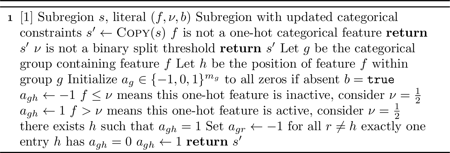
8.2.0.4 ImpliesTrue.
The routine ImpliesTrue determines whether a split condition \(f \le \nu\) is guaranteed to hold for all possible points in the subregion \(s\). For numerical features, this occurs when the upper bound of the interval satisfies \(u_f \le \nu\), meaning every feasible point lies on the True side. For categorical features, \(f \le \nu\) corresponds to the feature being \(0\). Thus, if the categorical status is \(-1\) (meaning the feature is forced to be \(0\)), the condition is always true. Otherwise, it is either always forced to be \(1\), or we do not know, so the outcome is not implied, and the routine returns false.

8.2.0.5 ImpliesFalse.
The routine ImpliesFalse determines whether a split condition \(f \le \nu\) is guaranteed to fail for all possible points in the subregion \(s\). For numerical features, this occurs when the lower bound satisfies \(\ell_f \ge \nu\), meaning all feasible points lie strictly on the False side. For categorical features, \(f \le \nu\) is always false precisely when the feature equals \(1\).
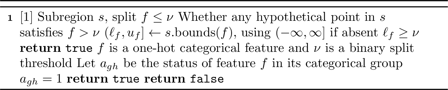
8.3 Compression into a Single Defer Tree↩︎
A compressed single-tree representation can substantially reduce root-to-leaf path lengths by specializing later-stage trees to the particular subregion in which they are evaluated. For example, a later-stage split such as \(\texttt{age} \le 23\) may help distinguish inputs in subregions with \(18 < \texttt{age} \le 25\) and \(\texttt{age} > 25\), but is redundant for any path already restricted to \(\texttt{age} \le 18\); when unrolling the MDT into a single tree, such splits can be pruned along the branches where they have no effect. On a high level, we will do this by putting the tree of stage \(i+1\) in the defer leaves of stage \(i\), simplifying it, and repeating once we reach the new defer leaves.
Algorithm 11 constructs a compressed single-tree representation of the full MDT by recursively expanding the staged decision process into one tree.
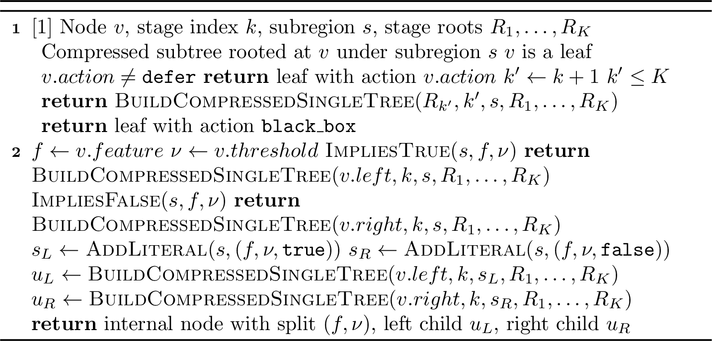
The procedure takes as input a node \(v\) from stage \(k\), along with a subregion \(s\) describing the set of inputs that may reach this node. The subregion \(s\) encodes all constraints accumulated along the path taken so far, potentially across multiple stages.
If \(v\) is a leaf, there are two cases. If the leaf corresponds to a terminal prediction (i.e., not defer), then the prediction is returned directly. If the leaf corresponds to defer, then we
transition to the next stage: we recurse on the root of stage \(k+1\) with the same subregion \(s\). If no further stages remain, we return a black_box leaf, representing the
final fallback model.
If \(v\) is an internal node with split \((f,\nu)\), we again leverage the subregion \(s\) to simplify the structure. If \(s\) provably implies that all possible inputs would satisfy the split (i.e., always take the True branch), then we recurse only on the left child. Similarly, if \(s\) implies the False branch, we recurse only on the right child. In either case, the split can be removed because it does not affect any possible point in the subregion.
Otherwise, the split is ambiguous under \(s\), and both branches must be explored. We construct refined subregions \(s_L\) and \(s_R\) by adding the corresponding literal to \(s\) (whether we are supposing we take the True or False branch), thereby capturing the additional constraint imposed by each branch. The algorithm then recursively builds the left and right subtrees under these refined subregions and returns a new internal node with these children.
8.4 Sequential Compression↩︎
In this section, we show how to (possibly) further compress a sequential representation of the MDT. Because the points outside the defer region are downweighted, it is somewhat unlikely that there exist splits in the MDT that provably do not separate any possible pair of points in the defer region; however, it is still possible. We note that compression of the sequential representation is exactly the compression done to reduce the number of literals in the rules of the rule list representation.
Algorithm 12 simplifies a tree relative to a set of possible incoming subregions \(\mathcal{S}\) (i.e., multiple defer leaves may lead to it, not just one). Intuitively, compared to constructing a single tree from the MDT, we must evaluate each split with respect to all subregions simultaneously, rather than a single input region.
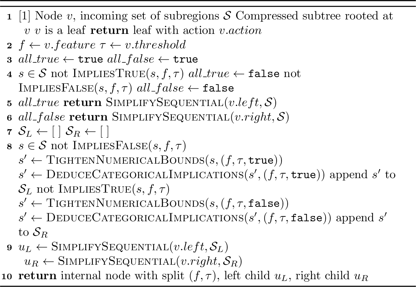
The procedure is recursive and begins at the root node. For each subregion \(s \in \mathcal{S}\), we determine whether the split always routes every possible input consistent with \(s\) (not just training samples, but any hypothetical point that satisfies the subregion constraints) to the True branch, the False branch, or whether the outcome is ambiguous (lines 8–15). If and only if every subregion is guaranteed to take the True branch, then \(\mathrm{\small all\_true}\) is set to True. Similarly, if and only if every subregion is guaranteed to take the False branch, then \(\mathrm{\small all\_false}\) is set to True. In either of these cases, the split can be pruned, and we recurse on the corresponding child. Otherwise, the split cannot be removed, and we must recurse on both branches.
In lines 24–34, we construct two (potentially overlapping) collections of subregions before recursing: \[\mathcal{S}_L = \left\{ \, s^{\le} \;:\; s \in \mathcal{S},\; s \text{ does not provably imply } f > t,\; s^{\le} \text{ is } s \text{ refined with } f \le t \right\},\] \[\mathcal{S}_R = \left\{ \, s^{>} \;:\; s \in \mathcal{S},\; s \text{ does not provably imply } f \le t,\; s^{>} \text{ is } s \text{ refined with } f > t \right\}.\]
Each collection is formed by selecting subregions that are compatible with the corresponding branch and refining them with the constraint induced by the split. Subregions that already contradict a branch are excluded from that side.
These two collections are not disjoint. Any subregion \(s\) that does not imply either outcome will appear in both sets (after being refined by the respective branch on which we recurse).
Algorithm 12 simplifies a tree as much as we provably can in this traversal when given a set of subregions that the tree will be used on. However, we still need to shrink this set of subregions before simplifying the next tree in the MDT.

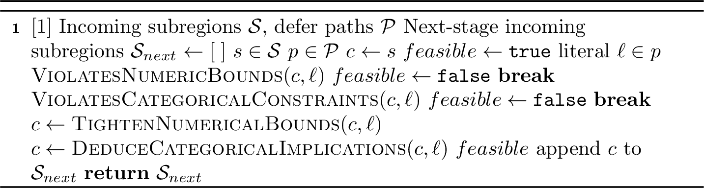
Algorithm 13 performs this update iteratively across stages. At stage \(k\), after simplifying the tree \(R_k\) into \(\widetilde{R}_k\), we identify all root-to-leaf paths that result in a defer decision. Each such path \(p \in \mathcal{P}\) corresponds to a conjunction of literals describing a
region of the input space that will be deferred by the current stage. To construct the subregions for the next stage, we combine the incoming subregions \(\mathcal{S}\) with these defer paths. Concretely, Algorithm 14 forms a Cartesian product between \(\mathcal{S}\) and \(\mathcal{P}\): for each subregion \(s \in
\mathcal{S}\) and each defer path \(p \in \mathcal{P}\), we attempt to extend \(s\) by sequentially incorporating the literals along \(p\). This
process can be viewed as intersecting the region represented by \(s\) with the region defined by the path \(p\). By adding one literal at a time, we allow for early termination. A
contradiction occurs if a literal violates the existing numerical bounds of the subregion or is incompatible with previously deduced categorical constraints. If any such violation occurs, the extended subregion is discarded. Otherwise, we tighten the
numerical bounds and propagate any implied categorical constraints, producing a refined subregion \(c\).
The resulting set \(\mathcal{S}_{next}\) therefore consists precisely of those subregions that are simultaneously: (i) reachable under the previous stages (captured by \(\mathcal{S}\)), and (ii) routed to deferral by the current stage (captured by \(\mathcal{P}\)).
8.5 Trivial Extensions↩︎
After recursively simplifying the left and right subtrees of a split, we may encounter a situation where both children reduce to identical leaf nodes with the same action. In this case, the split no longer affects the prediction for any input and can be safely removed. We refer to such splits as trivial extensions and perform this pruning as a post-order traversal at the end of any compression scheme.

9 Distance to Deferred Region↩︎
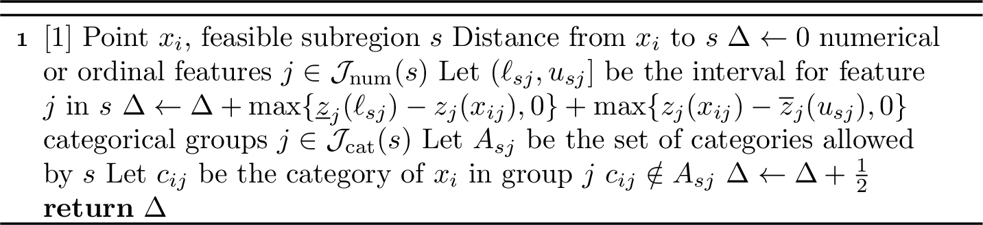
Each feasible subregion \(s \in \mathcal{S}_{k-1}\) stores the constraints induced by the current deferred region. Let \(\mathcal{J}_{\mathrm{num}}(s)\) denote the set of continuous (or ordinal) features that have been constrained in subregion \(s\), and let \(\mathcal{J}_{\mathrm{cat}}(s)\) denote the set of categorical feature groups that have been constrained. For each \(j \in \mathcal{J}_{\mathrm{num}}(s)\), let \((\ell_{sj}, u_{sj}]\) denote the interval induced by subregion \(s\). For each \(j \in \mathcal{J}_{\mathrm{cat}}(s)\), let \(A_{sj}\) denote the set of categories consistent (allowed by) with subregion \(s\). Additional details on handling categorical variables are provided in 8. At a high level, for a one-hot encoded categorical group, a subregion may rule out a category via a False split, leave it unconstrained, or identify it as active either through a True split or by eliminating all other categories. The categories which are consistent with the subregion are exactly the categories that are not ruled out by the subregion.
We first map each continuous or ordinal feature into its empirical quantile coordinate so that distances across coordinates are on a common scale. Since features may be discrete, we use the mid-rank empirical CDF, assigning each value \(v\) the quantile \[z_j(v) = \frac{\#\{X_j < v\} + \tfrac{1}{2}\#\{X_j = v\}}{N}.\]
Because interval endpoints may not coincide with observed feature values (e.g., midpoints), we evaluate endpoint quantiles by snapping to the nearest realized value that remains within the interval. Specifically, define \[\underline{z}_j(t) = \inf\{ z_j(v) : v > t,\;v \in \mathrm{supp}(X_j)\}, \qquad \overline{z}_j(t) = \sup\{ z_j(v) : v \le t,\;v \in \mathrm{supp}(X_j)\}.\]
Then, for each training point \(x_i\) that is not deferred, define its distance to the current deferred region by \[\textrm{defer\_dist}_{T_\textrm{{1:k-1}}}(x_i) = \min_{s \in \mathcal{S}_{k-1}} \left( \sum_{j \in \mathcal{J}_{\mathrm{num}}(s)} d_j^{(s)}(x_i) + \sum_{j \in \mathcal{J}_{\mathrm{cat}}(s)} d_j^{(s)}(x_i) \right).\]
For continuous (or ordinal) features \(j \in \mathcal{J}_{\mathrm{num}}(s)\), we measure distance in quantile space as \[d_j^{(s)}(x_i) = \max\{\underline{z}_j(\ell_{sj}) - z_j(x_{ij}), 0\} + \max\{z_j(x_{ij}) - \overline{z}_j(u_{sj}), 0\}.\]
For categorical features \(j \in \mathcal{J}_{\mathrm{cat}}(s)\), let \(c_{ij}\) denote the category of point \(x_i\) on feature \(j\). We define \[d_j^{(s)}(x_i) = \begin{cases} 0, & c_{ij} \in A_{sj},\\[4pt] \tfrac{1}{2}, & c_{ij} \notin A_{sj}. \end{cases}\]
This choice is consistent with treating a binary feature as continuous under the mid-rank empirical CDF, where a mismatch incurs a quantile distance of \(\tfrac{1}{2}\); we extend this to general categorical features.
Unconstrained features (i.e., \(j \notin \mathcal{J}_{\mathrm{num}}(s) \cup \mathcal{J}_{\mathrm{cat}}(s)\)) contribute zero distance as no value for them will change what leaf you are in.
Using these distances, we convert each \(\textrm{defer\_dist}_{T_\textrm{{1:k-1}}}(x_i)\) into a similarity score \[(1+\textrm{defer\_dist}_{T_\textrm{{1:k-1}}}(x_i))^{-\gamma}.\]
Let \(\mathcal{D}_{k-1} \subseteq \mathcal{X}\) denote the set of deferred points after stage \(k-1\). We define training weights \(w_i\) for the next iteration (on the first iteration, all weights are 1). \[w_i \;=\; \begin{cases} 1, & \text{if } x_i \in \mathcal{D}_{k-1} \\[6pt] (1 - \mu)\,(1 +\textrm{defer\_dist}_{T_\textrm{{1:k-1}}}(x_i))^{-\gamma}, & \text{if } x_i \notin \mathcal{D}_{k-1} \end{cases}\]
When \(\gamma=0\), this reduces to assigning a uniform weight of \(1-\mu\) to each non-deferred point and a weight of \(1\) to each deferred point.
10 Full Algorithm↩︎
10.1 MDT Algorithm↩︎
Algorithm 16 presents the full version of our algorithm. There are two additions relative to the algorithm presented in the main paper. The first is that we update the set of subregions \(\mathcal{S}\) (lines 4, 21, 22, 28) and pass it into our FilterSplits and GetWeights so it does not have to be recomputed from scratch each iteration. The second is that we additionally support early termination of training if the model complexity becomes too large. This is measured in 3 ways: (i) a stage of the tree has too many leaves, (ii) the sum of leaves across stages becomes too large, or (iii) the number of leaves in the naı̈ve representation of an MDT as a single tree becomes too large. (iii) takes advantage of a recurrence derived in Proposition 5. Given that we have already computed that tree, we choose to add it to MDT anyway, stopping after that.
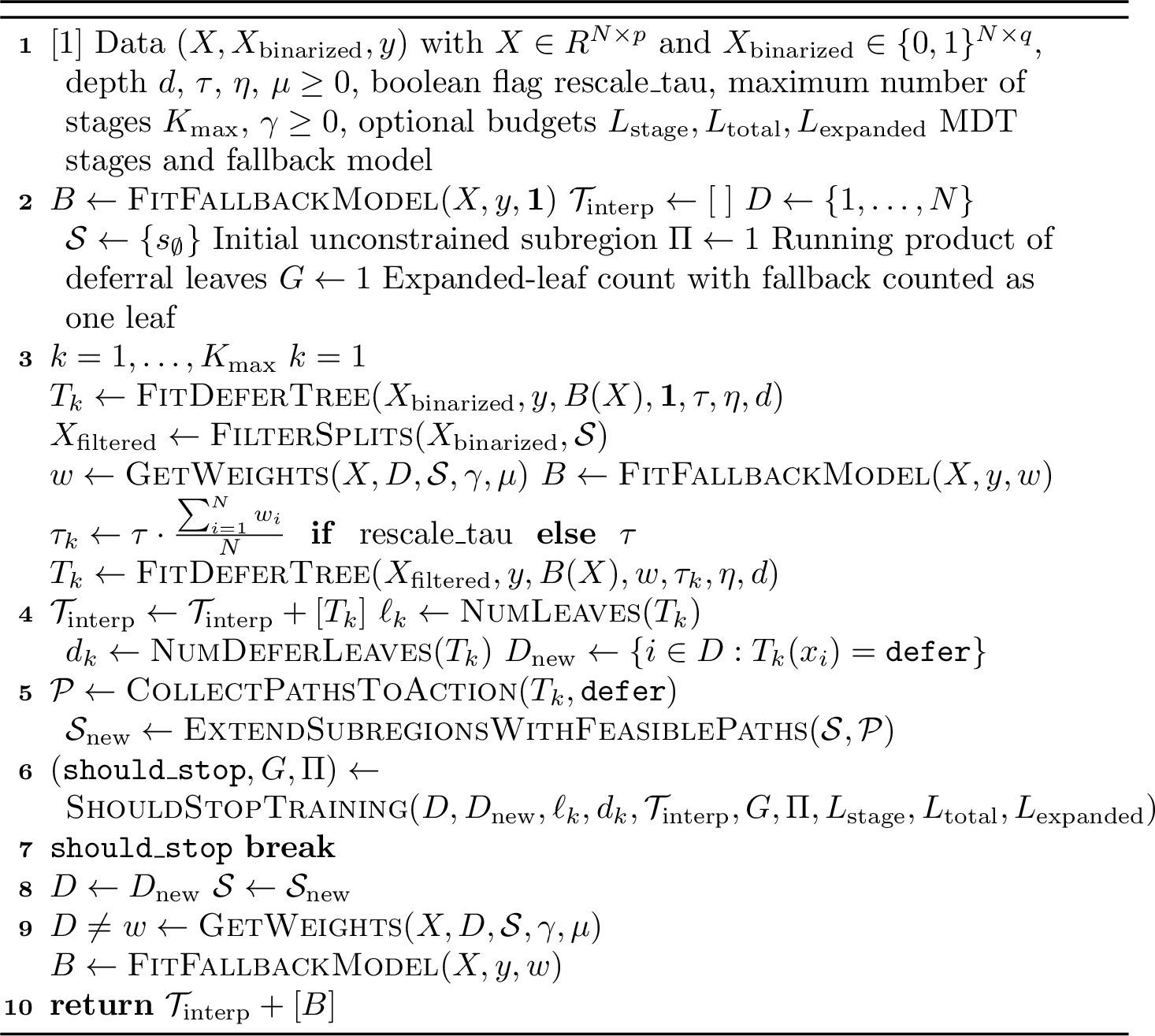
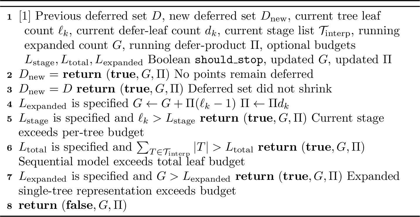
Algorithm 17 includes the aforementioned stopping criteria. It terminates training if the deferred set becomes empty, fails to shrink, or if any complexity budget is exceeded. The expanded tree size is tracked online using a recurrence, allowing early stopping without constructing a single tree representation.
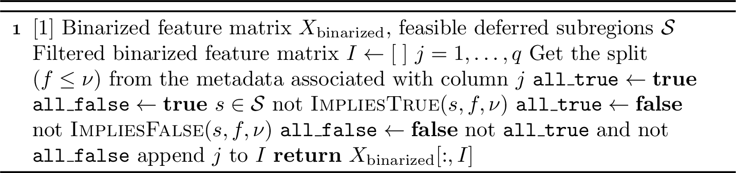
Algorithm 18 removes binary features that do not distinguish between feasible deferred subregions. A feature is discarded if it is provably always true or always false across all subregions (note that we can’t
discard a feature if it is provably true on half of the subregions and provably false on the others). This has the added bonus of reducing the search space, which is beneficial for near-optimal decision tree algorithms. We implement this by storing, for
each column, a string representation of the split (e.g., age<=25), which we parse to recover the feature and threshold. The column itself in the binarized dataset includes which samples satisfy the split.
Algorithm 19 assigns weights based on distance to the deferred region. Deferred points receive full weight, while non-deferred points are down-weighted according to their proximity to the nearest feasible subregion. This emphasizes points near the deferral boundary during training.

Algorithm 20 computes the distance from a point to a subregion by summing per-feature deviations. Numerical features are measured in quantile space, while categorical features incur a fixed penalty of \(\frac{1}{2}\) if the subregion does not allow the category that the point is in (i.e, the path to the subregion took a split of false on that category). Unconstrained features contribute zero.
10.2 Defer Tree Algorithm↩︎
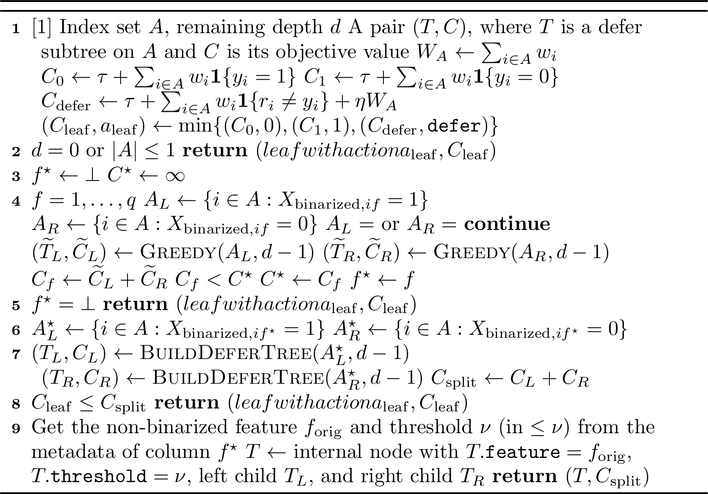
In Algorithm 21 construct each defer tree using a recursive, top-down procedure that jointly optimizes over prediction and deferral decisions. This algorithm uses the same heuristics to select splits as are used in the LicketySPLIT algorithm of [30]. Our implementation extends the efficient C++ codebase of [41], which implements a modified version of LicketySPLIT. Their algorithm considers an unweighted dataset and builds standard decision trees (without deferral). Our changes lie in supporting weights and deferral, thus optimizing a different objective. We solve the optimization problem using a per-leaf penalty, which is equivalent to optimizing a per-split penalty, since the number of leaves in a decision tree is always exactly one more than the number of splits, differing only by an additive constant \(\tau\).
At any node, we consider three possible leaf actions: predicting class \(0\), predicting class \(1\), or deferring to the fallback model. Each action is assigned an objective value that combines a fixed leaf penalty \(\tau\) with a weighted misclassification cost.
At a high level, we will recursively consider every possible split. We query a greedy method to build a subtree on the left and right child of every split, and choose the split that minimizes our objective under greedy completions. After choosing this split, we recurse on the left and right children of this split, and repeat.

The greedy subroutine (Algorithm 23) follows a very similar structure: it considers all splits and chooses the one that minimizes the weighted label entropy of the resulting partition (we minimize this quantity in Algorithm 24).
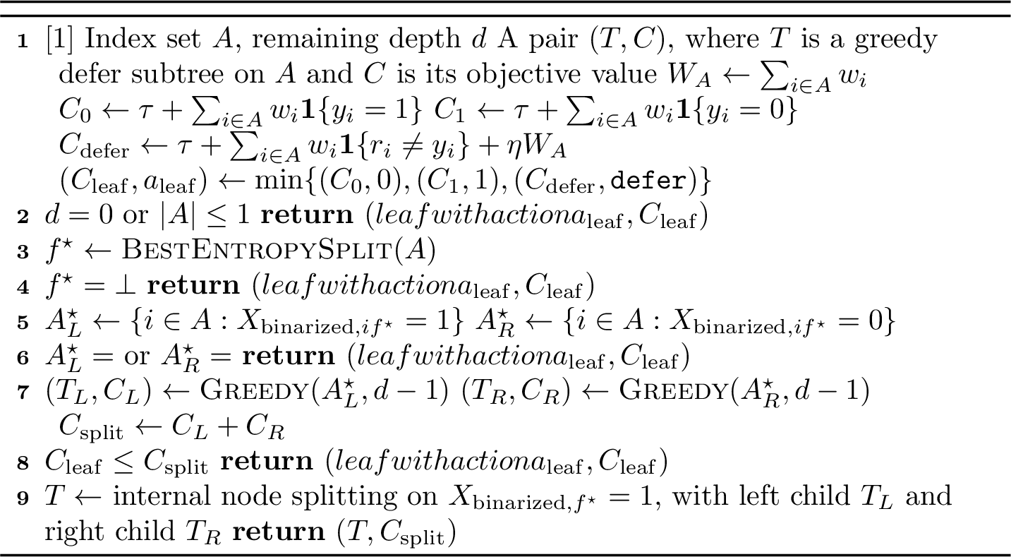
Algorithm 24 selects splits by minimizing the weighted label entropy of the resulting partition. This focuses on separating the labels rather than directly optimizing the defer-aware objective. As this is the standard heuristic in greedy decision tree algorithms, we adopt it here.

10.3 Improving Optimization with Backfitting↩︎
The MDT training procedure constructs the model as a sequence of defer trees that are trained with respect to a temporary black box fallback model (Algorithms 2 and 16). At the first stage, we train \(T_1\) to either predict or defer to an initial fallback model \(B_1\). After this stage identifies a remaining deferred region, we reweight the data toward that region, train a new fallback \(B_2\), and then train \(T_2\) to either predict or defer to \(B_2\). Continuing this process, we train \(T_i\) to defer to \(B_i\), but in the final model, \(T_i\) does not necessarily defer to \(B_i\). For instance, if there are 4 trees in the MDT, \(T_1\) defers to another MDT, not a black box.
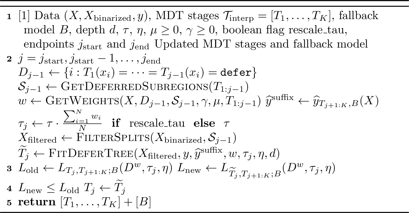
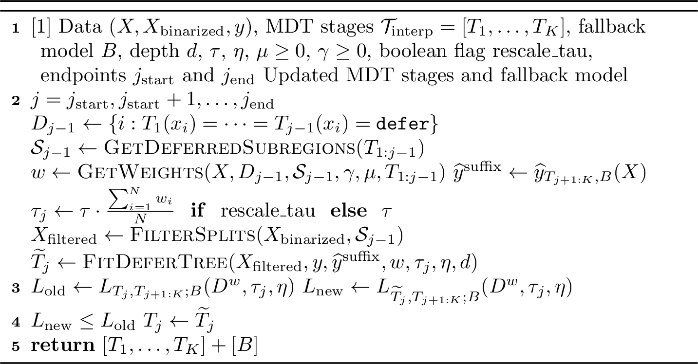
Therefore, once full MDT has been constructed, it may be beneficial to retrain stage \(j\) to defer to the entire suffix \(T_{j+1:K};B\). This motivates the following procedure: choose a component of the MDT, hold the rest of the model fixed, and retrain that component against the suffix that follows it. As we are optimizing using near-optimal algorithms, it will also be helpful to have an acceptance step to accept the new defer tree only if it is better in the objective that the algorithm tried to optimize.
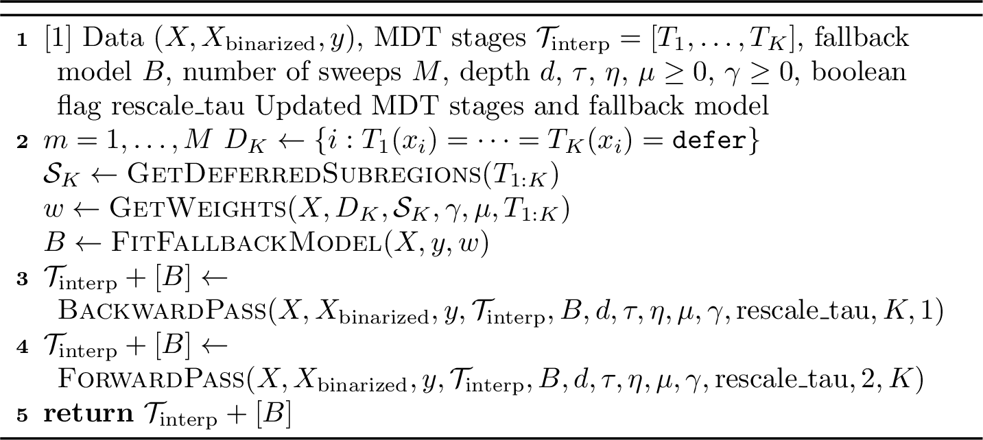
The backward pass (Algorithm 25) starts from the final fallback model and moves upstream through the MDT, retraining each stage conditioned on the rest of it. We then visit stages in reverse order (optionally starting with the fallback model) doing exactly that. In contrast, the forward pass (Algorithm 26) does exactly the same thing but it starts from the first stage. We put these together in an alternating approach (Algorithm 27). It combines these two sweeps in the following update order: \(B,\;T_K,T_{K-1},\ldots,T_1,\;T_2,T_3,\ldots,T_K,\ldots\). The results of using this approach are shown in 37. In short, backfitting gives clear improvements on some datasets, such as Tictactoe, where revisiting stages may help capture higher-order interactions, but it degrades performance on several others.
11 Training Objectives↩︎
Learning a sparse decision tree is commonly formulated as minimizing a regularized empirical risk of the form
\[\frac{1}{N}\sum_{i=1}^N \mathbb{1}\{T(x_i) \neq y_i\} + \lambda |T|,\]
where \(|T|\) is the number of leaves in the tree [25], [30], [36]. For binary trees, the number of internal split nodes is always \(|T|-1\). Therefore, minimizing a penalty on leaves is equivalent, up to an additive constant \(\lambda\), to minimizing a penalty on split nodes:
\[\frac{1}{N}\sum_{i=1}^N \mathbb{1}\{T(x_i) \neq y_i\} + \lambda |T| = \frac{1}{N}\sum_{i=1}^N \mathbb{1}\{T(x_i) \neq y_i\} + \lambda (|T|-1) + \lambda.\]
Since the two objectives differ only by a constant term, they have the same set of minimizers. We choose to work with the number of splits for a reason that will become clear in the MDT objective.
Hybrid interpretable rule-list models instead optimize an objective that balances the error of the full hybrid system, the complexity of the interpretable rule list, and the amount of deferral to a black-box model. In the notation of [7], for a rule list \(r\) and black box \(B\), this objective has the form \[\frac{\widehat L_{\mathcal{D}}(B,r)}{N} + \lambda |r| + \beta \frac{|\mathcal{D} \setminus \mathcal{D}_r|}{N},\] where \(\widehat L_{\mathcal{D}}(B,r)\) is the empirical error of the full hybrid model, \(|r|\) is the number of rules, and \(\mathcal{D}_r\) is the subset of samples captured by the rule list. Equivalently, \(|\mathcal{D} \setminus \mathcal{D}_r|/N\) is the empirical deferral rate.
Our single defer tree objective combines these two perspectives. It is a sparse decision tree objective combined with a soft penalty for deferral: \[\mathcal{L}_{T,B}(\mathcal{D}^w,\tau,\eta) = \tau(|T|-1) + \sum_{i=1}^N w_i \left( \mathbb{1}\{\hat{y}_{T,B}(x_i)\neq y_i\} + \eta \mathbb{1}\{T(x_i)=\mathrm{defer}\} \right).\]
When all weights are \(w_i=1\) and \(\eta=0\), we recover the same loss (except we do not normalize by the dataset size \(N\)) as [25], [30], [36], with \(\tau = \lambda N\).
The MDT objective is then the natural extension of the single defer-tree objective: it penalizes the predictions and deferral rate after routing through all stages of the MDT. \[\mathcal{L}_{T_{1:k},B}(\mathcal{D}^w,\tau,\eta) = \tau \sum_{j=1}^k (|T_j|-1) + \sum_{i=1}^N w_i \left( \mathbb{1}\{\hat{y}_{T_{1:k},B}(x_i)\neq y_i\} + \eta \mathbb{1}\{T_{1:k}(x_i)=\mathrm{defer}\} \right).\] When \(k=1\), this reduces exactly to the single defer-tree objective. For MDTs, it is more natural to regularize the number of splits rather than leaves because if there was a stage with a single defer leaf, regularizing by the number of leaves would increase the MDT objective, though nothing was changed about the predictions or the amount that the MDT deferred.
Finally, Theorem [thm:rule-list] shows that any MDT has an associated rule-list representation with \[|r_{\mathrm{MDT}}| = \sum_{j=1}^k (|T_j|-d_j),\] where \(|T_j|\) is the number of leaves of stage \(j\) and \(d_j\) is the number of deferral leaves in that stage. Assume the MDT has a non-zero deferral rate to the fallback model: this means that every stage defers. Since \(d_j\geq 1\), \[\sum_{j=1}^k (|T_j|-d_j) \leq \sum_{j=1}^k (|T_j|-1)\] Therefore, the MDT split penalty upper bounds the rule-list sparsity penalty of the corresponding rule-list representation.
12 Experiment Setup↩︎
12.1 Machines↩︎
All experiments were performed on an institutional computing cluster. Each experiment was executed on a single compute node equipped with an AMD EPYC 9554 processor (2.75 GHz), with 64 physical cores. Resources were restricted to 1 CPU core and 50 GB of RAM.
12.2 Datasets↩︎
We provide a description of all datasets used in this work and the binary classification task we chose.
For all datasets, we remove rows containing missing values and one-hot encode all categorical variables.
12.2.0.1 Abalone [42] (4,177 samples)
Predict whether an abalone is male based on its physical measurements.
12.2.0.2 Adult [43] (48,842 samples)
Predict whether an individual earns more than $50,000 per year based on demographic and occupational attributes.
12.2.0.3 Aging [44], [45] (714 samples)
Predict whether an individual has visited at least two doctors.
12.2.0.4 Bike [46], [47] (17,379 samples)
Predict whether bike rental demand exceeds the median.
12.2.0.5 California [48] (20,634 samples)
Predict whether the provided binary target variable price is true.
12.2.0.6 Churn [49], [50] (5,000 samples)
Predict whether a customer will churn.
12.2.0.7 Compas [51] (4,966 samples)
Predict whether a defendant will recidivate within two years.
12.2.0.8 Coupon [52] (108 samples)
Predict whether an individual accepts a recommended coupon.
12.2.0.9 Credit [53], [54] (30,000 samples)
Predict whether a client will default on their credit card payment in the following month.
12.2.0.10 Diamonds [55] (53,940 samples)
Predict whether a diamond belongs to cut category 2 based on its physical attributes.
12.2.0.11 Droid [56], [57] (29,332 samples)
Predict whether an Android application is malicious.
12.2.0.12 Heloc [58] (2,502 samples)
Predict whether an individual is high- or low-risk for a home equity line of credit.
12.2.0.13 Jasmine [59], [60] (2,984 samples)
Binary classification using the provided target column.
12.2.0.14 Madeline [61] (3,140 samples)
Binary classification using the provided target column.
12.2.0.15 Magic [62] (19,020 samples)
Predict whether a Cherenkov telescope image corresponds to a gamma ray or background noise.
12.2.0.16 Monk2 [63], [64] (601 samples)
Predict the logical rule where the label is 1 if exactly two of six attributes take value 1.
12.2.0.17 Phishing [65], [66] (11,055 samples)
Predict whether a website is phishing or legitimate.
12.2.0.18 Pol [67] (10,082 samples)
Binary classification using the provided target column.
12.2.0.19 Rl [68] (4,970 samples)
Binary classification using the provided target column.
12.2.0.20 Shopping [69], [70] (12,330 samples)
Predict whether an online shopping session ends in a purchase.
12.2.0.21 Spambase [71] (4,601 samples)
Predict whether an email is spam.
12.2.0.22 Student [72], [73] (649 samples)
Predict whether a student passes a course (final grade \(\geq 10\)).
12.2.0.23 Tic-Tac-Toe [74] (958 samples)
Predict whether a player has won given a terminal board configuration.
12.2.0.24 Wine [75] (6,497 samples)
Predict whether wine quality is at least 7.
12.3 Hyperparameter Selection↩︎
All cross-validation was done with 3 folds. Any results reported are averaged across 5 train/test splits.
12.3.1 Black Boxes:↩︎
12.3.1.1 Random Forest.
Random Forest hyperparameters were tuned with Optuna using a 12-hour timeout per train/test split: \[\begin{align} n_{\text{estimators}} &\in \{100,200,\ldots,1200\},\\ \text{max\_depth} &\in [2,32],\\ \text{min\_samples\_split} &\in [2,40],\\ \text{min\_samples\_leaf} &\in [1,20],\\ \text{max\_features} &\in \{\sqrt{p}, \log_2(p), \alpha p:\alpha\in[0.1,1.0]\},\\ \text{bootstrap} &\in \{\text{True},\text{False}\},\\ \text{class\_weight} &\in \{\text{None},\text{balanced},\text{balanced\_subsample}\}. \end{align}\]
12.3.1.2 XGBoost.
XGBoost hyperparameters were tuned with Optuna using a 12-hour timeout per train/test split: \[\begin{align} n_{\text{estimators}} &\in \{100,200,\ldots,1200\},\\ \text{max\_depth} &\in [2,12],\\ \text{learning\_rate} &\in [10^{-3},3\cdot 10^{-1}] \text{ on a log scale},\\ \text{min\_child\_weight} &\in [10^{-2},20] \text{ on a log scale},\\ \text{subsample} &\in [0.5,1.0],\\ \text{colsample\_bytree} &\in [0.5,1.0],\\ \gamma &\in [10^{-8},10] \text{ on a log scale},\\ \alpha_{\text{reg}} &\in [10^{-8},10] \text{ on a log scale},\\ \lambda_{\text{reg}} &\in [10^{-8},10] \text{ on a log scale}. \end{align}\]
12.3.2 Additive Models with Pairwise Interactions↩︎
12.3.2.1 Explainable Boosting Machine (EBM).
EBM hyperparameters were tuned with Optuna using a 12-hour timeout per train/test split and 5-fold cross-validation: \[\begin{align} \text{interactions} &\in [0,50],\\ \text{learning\_rate} &\in [10^{-3},5\cdot 10^{-2}] \text{ on a log scale},\\ \text{max\_rounds} &\in \{200,400,\ldots,5000\},\\ \text{max\_bins} &\in \{64,128,256,512,1024\},\\ \text{max\_interaction\_bins} &\in \{16,32,64,128\},\\ \text{min\_samples\_leaf} &\in [2,50],\\ \text{max\_leaves} &\in [2,5],\\ \text{outer\_bags} &\in \{4,8,12,16\},\\ \text{validation\_size} &\in \{0.10,0.15,0.20\},\\ \text{early\_stopping\_rounds} &\in \{50,100,200\},\\ \text{early\_stopping\_tolerance} &\in [10^{-6},10^{-3}] \text{ on a log scale}. \end{align}\]
12.3.3 Sparse Ensembles↩︎
12.3.3.1 FIGS.
FIGS hyperparameters were tuned with Optuna using a 12-hour timeout per train/test split. The following search space was used: \[\begin{align} \text{max\_rules} &\in [4,64],\\ \text{max\_trees} &\in [2,20],\\ \text{max\_depth} &\in [2,12],\\ \text{max\_features} &\in \{\text{None}, \sqrt{p}, \log_2(p)\},\\ \text{min\_impurity\_decrease} &\in [10^{-8},10^{-4}] \text{ on a log scale}. \end{align}\] The interpretability constraints \(\text{max\_rules} \le 64\), \(\text{max\_trees} \le 20\), and \(\text{max\_depth} \le 12\) were always enforced.
12.3.4 Interpretable Models↩︎
12.3.4.1 SingleTree.
For a single decision tree algorithm, we used our DeferTree algorithm with \(\eta=10^9\) to ensure no deferral (we also verified this on all results reported). This corresponds to a version of the near-optimal decision tree algorithm LicketySPLIT [30].
\[\begin{align} \lambda &\in \{10^{-5},5\cdot 10^{-5},10^{-4},5\cdot 10^{-4},10^{-3},5\cdot 10^{-3},10^{-2}\},\\ \end{align}\] We fixed a depth budget of \(10\), using \(\lambda\) to grow a sparser tree. This method requires a binarized dataset. We binarized the dataset with ThresholdGuessing [36], using \(n_{\text{estimators}} = 150\) and \(\text{max\_depth} = 2\).
12.3.5 Hybrid Models↩︎
12.3.5.1 HyRS.
For HyRS, we tuned \[\begin{align} \text{nrules} &\in \{5000\},\\ \text{supp} &\in \{5,20\},\\ \text{maxlen} &\in \{2,3\},\\ \alpha &\in \{10^{-4},10^{-3},10^{-2}\},\\ \beta &\in \{0.01,0.05,0.10,0.15,0.25,0.50\},\\ \text{niter} &\in \{5000\}. \end{align}\] Non-binary numeric features were binarized using \(10\) quantile levels. We used their provided Random Forest rule mining approach.
12.3.5.2 FLMM.
For FLMM, we tuned \[\begin{align} r_{\max} &\in \{1,2,3\},\\ \ell &\in \{0.01,0.02,0.05,0.1,0.2\},\\ s &\in \{0.5,0.6,0.7,0.8,0.9,1.0\},\\ \text{min\_support\_frac} &\in \{0.005,0.01,0.02\}. \end{align}\]
We could not find an exact description of the rule mining done in [8], except that \(r_{\max}\) was tuned in \(\{1,2,3\}\). Therefore, we use the following procedure.
Non-binary numeric features were binarized using \(10\) quantile levels. Then, candidate rules were exhaustively enumerated as all conjunctions of between \(1\) and \(r_{\max}\) binary indicators. Any rule whose support was below \[\max\!\left(1,\left\lceil \text{min\_support\_frac}\cdot n \right\rceil\right)\] was discarded. For each remaining conjunction, the predicted label was chosen as the majority class among covered samples. Duplicate rules inducing identical coverage and prediction behavior were removed.
12.3.5.3 HybridCORELS-POST.
For the HybridCORELS-POST variant, we tuned \[\begin{align} c &\in \{0.001,0.01,0.1\},\\ \text{min\_coverage} &\in \{0.1,0.25,0.5,0.75,0.9\},\\ \text{max\_card} &\in \{1,2\},\\ \text{min\_support} &\in \{1,5\},\\ \text{n\_rules} &\in \{300\},\\ \end{align}\]
12.3.5.4 HybridCORELS-PRE.
For the HybridCORELS-PRE variant, we tuned \[\begin{align} c &\in \{0.001,0.01,0.1\},\\ \text{min\_coverage} &\in \{0.1,0.25,0.5,0.75,0.9\},\\ \text{max\_card} &\in \{1,2\},\\ \text{min\_support} &\in \{5\},\\ \text{n\_rules} &\in \{300\},\\ \alpha &\in \{0,5,10\}. \end{align}\]
For both optimal methods (HybridCORELS PRE and POST), we set a time limit of 10 minutes per hyperparameter to fit the rule list. This does not include training the black box or performing rule mining.
For the HybridCORELS variants, we first binarized the dataset with ThresholdGuessing [36], using \(n_{\text{estimators}} = 150\) and \(\text{max\_depth} = 2\). We then used their provided rule mining method on these binary features, which uses FPGrowth. Because the HybridCORELS implementation
exposes prediction through a predict method that accepts only the already rule-mined dataset, the fallback XGBoost model was required to operate on this same mined feature space. As such, we retuned the XGBoost model for each hyperparameter
combination for HybridCORELS, because the HybridCORELS hyperparameters can change the rule mining and thus what XGBoost is trained on. Aside from that, the method of choosing hyperparameters is discussed in 12.4.
12.3.5.5 DeferTree.
For our DeferTree, we tuned \[\begin{align} \lambda &\in \{10^{-5},5\cdot 10^{-5},10^{-4},5\cdot 10^{-4},10^{-3},5\cdot 10^{-3},10^{-2}\},\\ \eta &\in \{0.001,0.005,0.01,0.05,0.1,0.3,0.6,0.8,1.0,10^9\}. \end{align}\]
This method requires a binarized dataset. We binarized the dataset with ThresholdGuessing [36], using \(n_{\text{estimators}} = 150\) and \(\text{max\_depth} = 2\).
12.3.5.6 MDT.
For our MDT, we tuned \[\begin{align} \lambda &\in \{10^{-5},5\cdot 10^{-5},10^{-4},5\cdot 10^{-4},10^{-3},5\cdot 10^{-3},10^{-2}\},\\ \eta &\in \{0.001,0.005,0.01,0.05,0.1,0.3,0.6,0.8,1.0\},\\ \text{rescale\_tau} &\in \{0,1\},\\ c &\in \{0,0.2,0.5,1.0\},\\ \gamma &\in \{0,1,2,4,8\},\\ \end{align}\] The fixed settings were depth budget \(10\), maximum stages \(6\), maximum total stage leaves \(500\), maximum leaves in an uncompressed single tree \(10^6\), and maximum leaves per tree \(129\). In practice, we do not hit depth 10 or anywhere near these limits (shown in Figure [fig:sparsity95cdf95eps0025]); these are upper bounds that would only prune very undesired hyperparameters. In our algorithm, the calls to fit a DeferTree require a binarized dataset. We binarized the dataset with ThresholdGuessing [36], using \(n_{\text{estimators}} = 150\) and \(\text{max\_depth} = 2\).
12.4 Cross Validation Procedure↩︎
For hybrid interpretable models with fallback black boxes, hyperparameter selection was performed separately for each dataset train/test split. For a given train/test split, we constructed a table whose rows corresponded to hybrid-model hyperparameter combinations and whose columns stored the average validation accuracy, average validation deferral rate, test accuracy, and test deferral rate.
To populate this table, we first created three subtrain/validation partitions from the training set. For each subtrain partition, we independently tuned an XGBoost model over the ranges described earlier using an inner 3-fold cross-validation procedure restricted to that subtrain partition. After selecting the best XGBoost hyperparameters for that subtrain partition, we fixed that XGBoost model and evaluated every hyperparameter combination in the hybrid interpretable grid using the associated validation split. Repeating this process across the three subtrain/validation partitions yielded an average validation accuracy and average validation deferral rate for each hybrid hyperparameter configuration.
Next, we tuned XGBoost once more on the entire training set using the same XGBoost search procedure. The resulting XGBoost model was then used as the fallback model for every hybrid hyperparameter configuration trained on the full training set, producing a corresponding test accuracy and test deferral rate.
Given this matrix for a dataset train/test split, if we wished to select the best model subject to at most \(x\%\) test deferral, we first filtered out all hyperparameter configurations whose test deferral exceeded the threshold. Among the remaining configurations, we selected the one with the highest average validation accuracy. We then reported the corresponding test accuracy and test deferral for that configuration. We note that the former (the test accuracy) had not been looked at before then, and was not used to choose any hyperparameters. This entire procedure was repeated independently across the five train/test splits for each dataset.
13 Experimental Results↩︎
| Dataset | Defer Tree Non-Deferred Error | Defer Tree Deferred Error |
|---|---|---|
| Bike | 1.57% \(\pm\) 0.42% | 14.88% \(\pm\) 2.35% |
| Churn | 3.04% \(\pm\) 0.33% | 14.16% \(\pm\) 4.21% |
| Compas | 31.59% \(\pm\) 2.11% | 36.24% \(\pm\) 1.08% |
| Heloc | 25.59% \(\pm\) 2.61% | 36.43% \(\pm\) 6.78% |
| Jasmine | 13.97% \(\pm\) 2.46% | 32.39% \(\pm\) 4.45% |
| Phishing | 0.68% \(\pm\) 0.24% | 11.84% \(\pm\) 1.54% |
| Pol | 0.07% \(\pm\) 0.08% | 6.56% \(\pm\) 0.81% |
| RL | 16.57% \(\pm\) 2.30% | 24.34% \(\pm\) 2.99% |
| Wine | 4.67% \(\pm\) 0.88% | 19.49% \(\pm\) 1.51% |
In 28, we compare the semi-supervised hyperparameter selection procedure to a variant that uses training deferral rate as a proxy for test deferral rate. We utilized this semi-supervised procedure for all methods, and here we compare this approach to using the train deferral rate for MDT+XGB. For each target deferral level \(x\), we choose the hyperparameters with the highest average validation accuracy among those with deferral rate at most \(x\), where deferral is measured on the test set for MDT+XGB and on the training set for MDT+XGB Train. After selecting hyperparameters separately for each of the five train/test splits, we plot the average test accuracy against the average test deferral rate of the selected models. Across datasets, the two curves are nearly indistinguishable: using training deferral is sometimes slightly better and sometimes slightly worse, but it usually selects models with essentially the same test accuracy–deferral tradeoff. The only clear degradation occurs on Coupon, which has only 108 total samples after removing missing values, so little weight should be placed on that outlier. Overall, these results suggest that training deferral rate is an acceptable practical proxy for test deferral rate when selecting MDT+XGB hyperparameters.
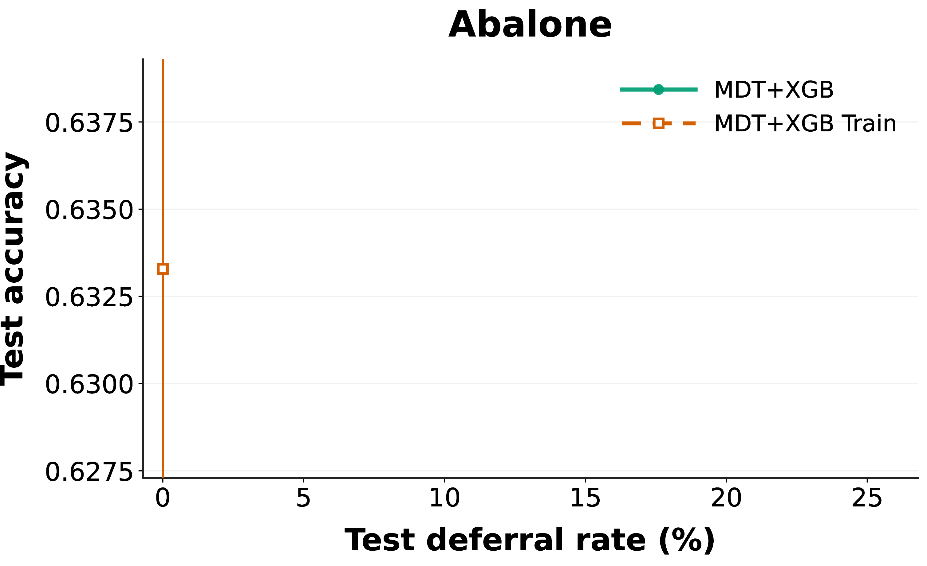
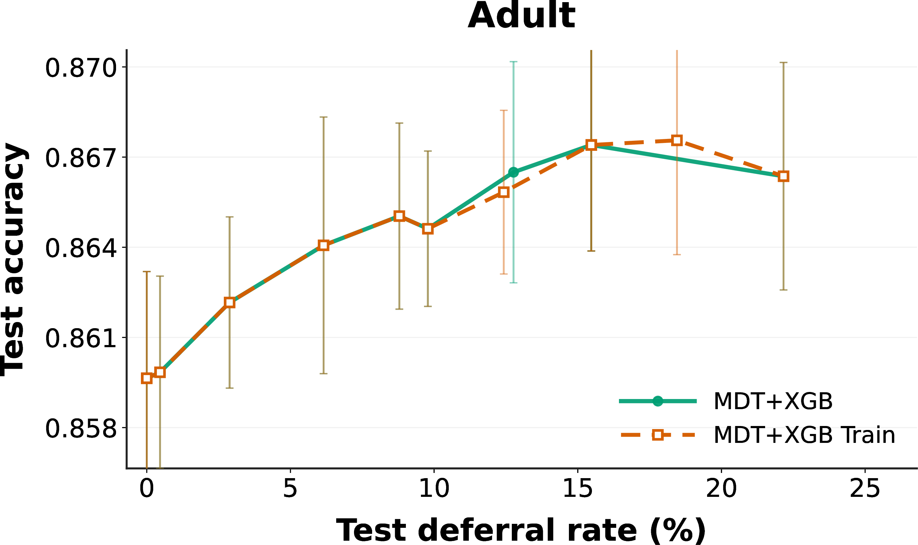
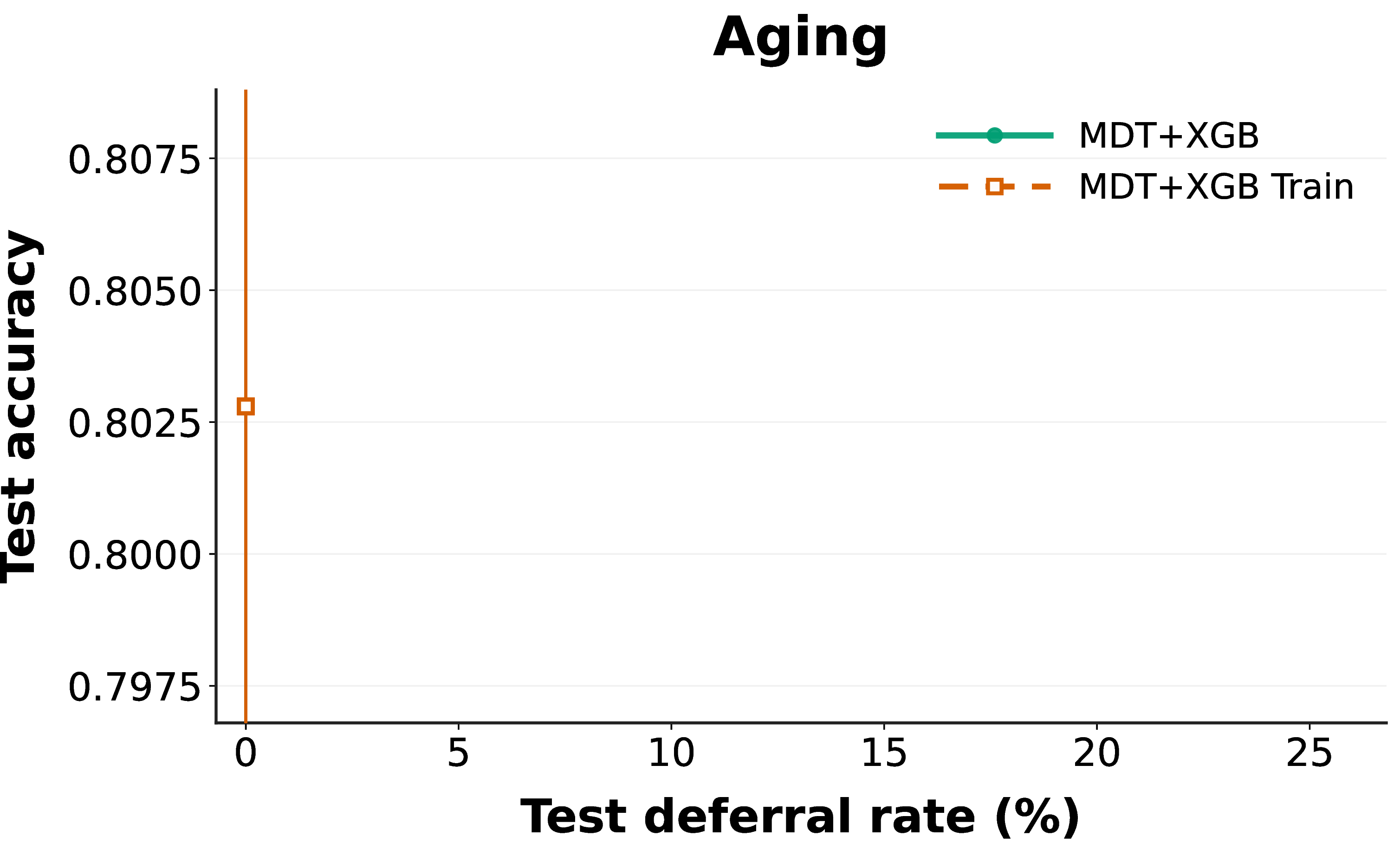
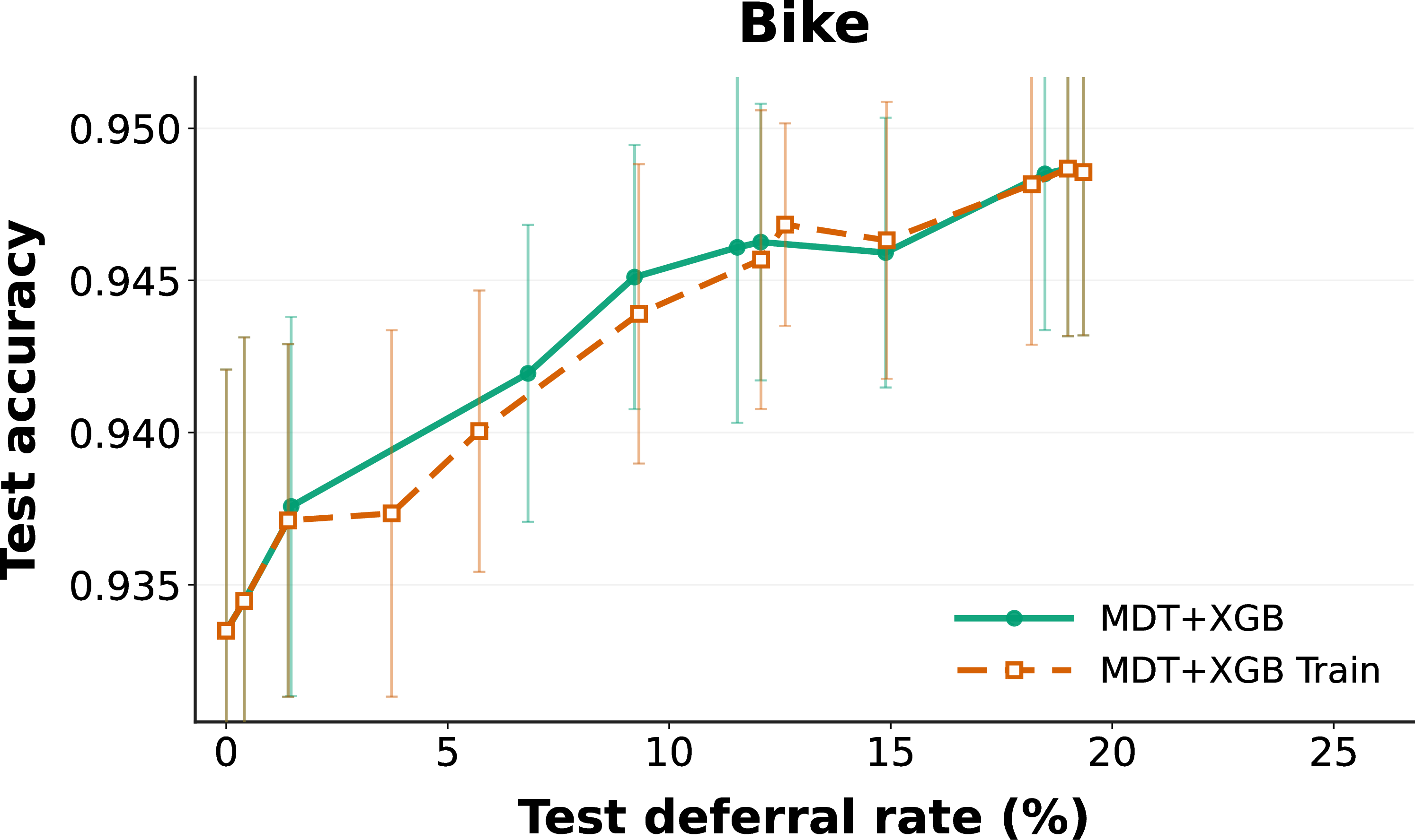


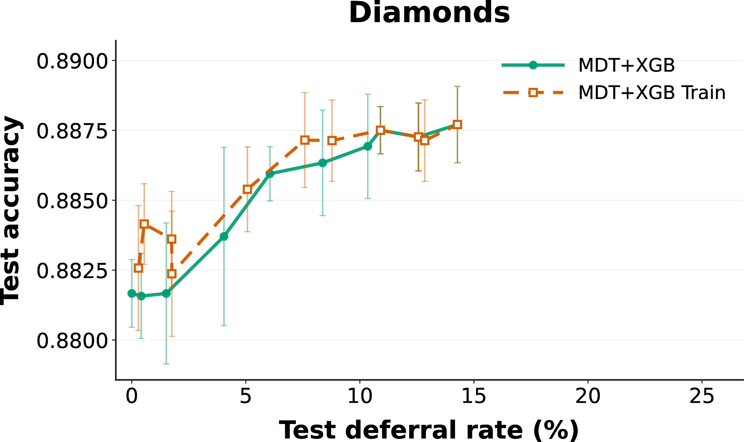
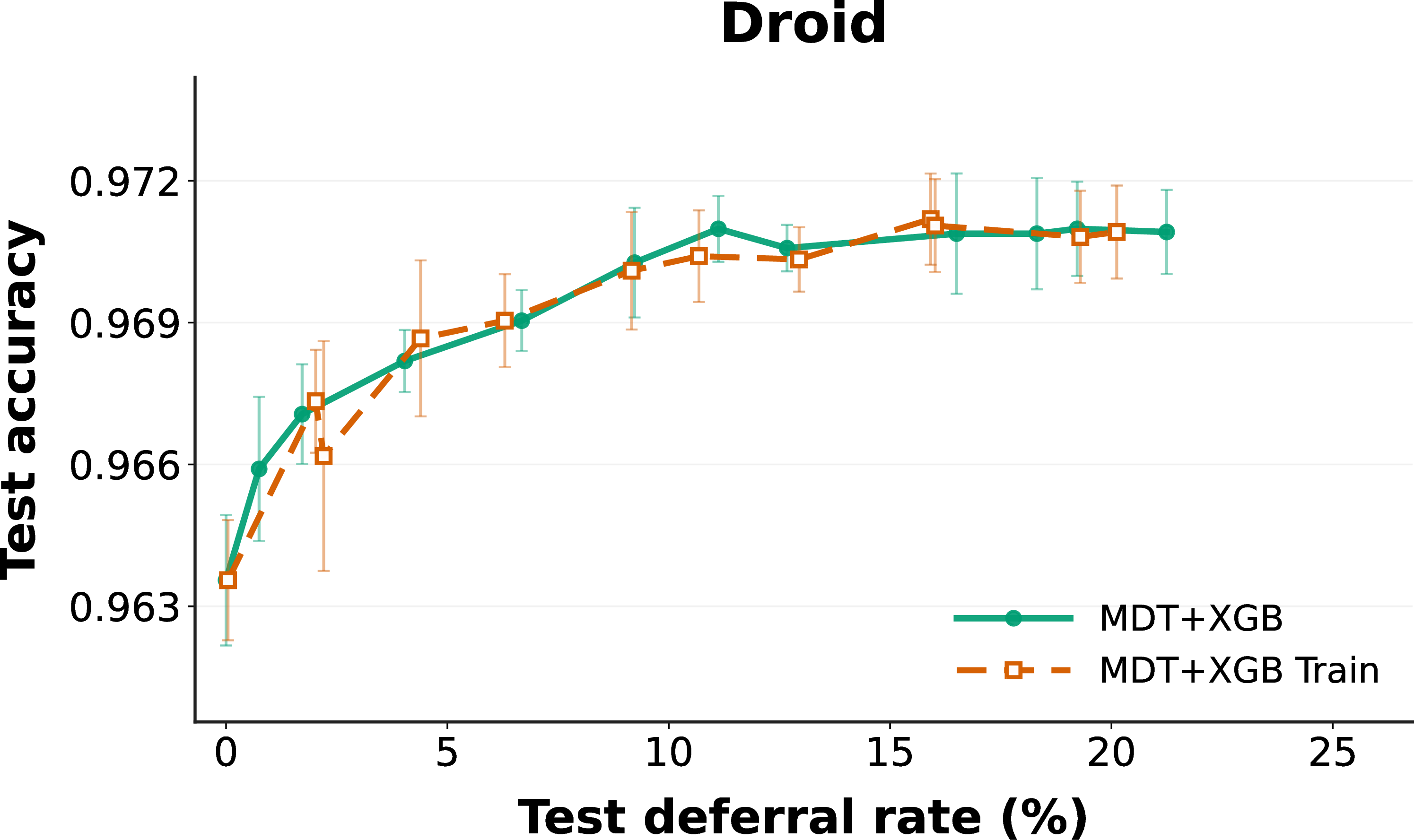
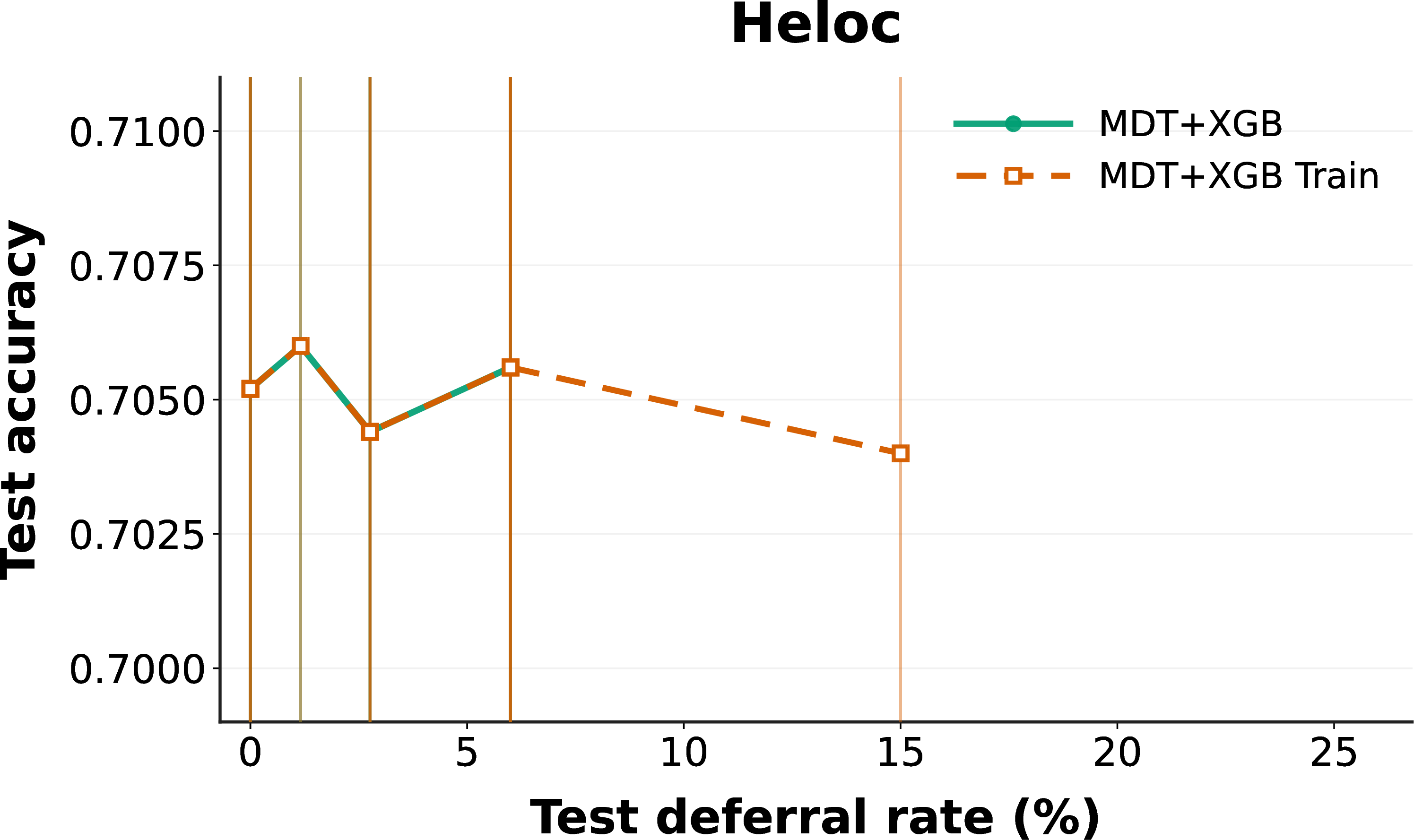
Figure 28: Comparison between MDT+XGB hyperparameter selection using test deferral rate and selection using training deferral rate..
| Dataset | Difference in Train/Test Defer Rates | Train Defer Rate | Test Defer Rate |
|---|---|---|---|
| Abalone | \(0.0000 \pm 0.0000\) | \(0.0000 \pm 0.0000\) | \(0.0000 \pm 0.0000\) |
| Adult | \(0.0052 \pm 0.0046\) | \(0.2176 \pm 0.0307\) | \(0.2216 \pm 0.0309\) |
| Aging | \(0.0000 \pm 0.0000\) | \(0.0000 \pm 0.0000\) | \(0.0000 \pm 0.0000\) |
| Bike | \(0.0055 \pm 0.0047\) | \(0.1595 \pm 0.0399\) | \(0.1539 \pm 0.0397\) |
| California | \(0.0105 \pm 0.0073\) | \(0.2208 \pm 0.0142\) | \(0.2110 \pm 0.0218\) |
| Churn | \(0.0037 \pm 0.0040\) | \(0.0508 \pm 0.0556\) | \(0.0532 \pm 0.0544\) |
| Compas | \(0.0084 \pm 0.0102\) | \(0.1240 \pm 0.1148\) | \(0.1225 \pm 0.1137\) |
| Coupon | \(0.0142 \pm 0.0317\) | \(0.0233 \pm 0.0520\) | \(0.0091 \pm 0.0203\) |
| Credit | \(0.0043 \pm 0.0029\) | \(0.0731 \pm 0.0689\) | \(0.0730 \pm 0.0721\) |
| Diamonds | \(0.0043 \pm 0.0029\) | \(0.1658 \pm 0.0450\) | \(0.1624 \pm 0.0479\) |
| Droid | \(0.0033 \pm 0.0021\) | \(0.1841 \pm 0.0621\) | \(0.1841 \pm 0.0648\) |
| Heloc | \(0.0105 \pm 0.0118\) | \(0.0495 \pm 0.0555\) | \(0.0600 \pm 0.0671\) |
| Jasmine | \(0.0067 \pm 0.0072\) | \(0.0613 \pm 0.0729\) | \(0.0593 \pm 0.0782\) |
| Madeline | \(0.0139 \pm 0.0105\) | \(0.1150 \pm 0.0843\) | \(0.1102 \pm 0.0811\) |
| Magic | \(0.0027 \pm 0.0023\) | \(0.2299 \pm 0.0129\) | \(0.2301 \pm 0.0128\) |
| Monk2 | \(0.0000 \pm 0.0000\) | \(0.0000 \pm 0.0000\) | \(0.0000 \pm 0.0000\) |
| Phishing | \(0.0109 \pm 0.0061\) | \(0.1807 \pm 0.0300\) | \(0.1873 \pm 0.0376\) |
| Pol | \(0.0033 \pm 0.0036\) | \(0.1474 \pm 0.0497\) | \(0.1463 \pm 0.0524\) |
| Rl | \(0.0094 \pm 0.0079\) | \(0.1520 \pm 0.0609\) | \(0.1441 \pm 0.0617\) |
| Shopping | \(0.0057 \pm 0.0041\) | \(0.2056 \pm 0.0277\) | \(0.2015 \pm 0.0250\) |
| Spambase | \(0.0146 \pm 0.0124\) | \(0.1717 \pm 0.0349\) | \(0.1863 \pm 0.0301\) |
| Student | \(0.0084 \pm 0.0157\) | \(0.0470 \pm 0.0880\) | \(0.0554 \pm 0.1037\) |
| Tictactoe | \(0.0047 \pm 0.0065\) | \(0.0350 \pm 0.0346\) | \(0.0323 \pm 0.0358\) |
| Wine | \(0.0124 \pm 0.0102\) | \(0.2101 \pm 0.0539\) | \(0.1982 \pm 0.0465\) |
4pt
| Dataset | Split Compression | Leaf Compression | MDT Deferred Accuracy | XGB Deferred Accuracy | \(\Delta\) Accuracy (MDT \(-\) XGB) |
|---|---|---|---|---|---|
| Adult | \(1.0214 \pm 0.0167\) | \(1.0819 \pm 0.0556\) | \(0.7049\;[0.6959, 0.7139]\) | \(0.7067\;[0.6977, 0.7156]\) | \(-0.0018\;[-0.0048, 0.0012]\) |
| Bike | \(1.0642 \pm 0.0277\) | \(1.0875 \pm 0.0803\) | \(0.8082\;[0.7933, 0.8228]\) | \(0.8090\;[0.7940, 0.8236]\) | \(-0.0007\;[-0.0060, 0.0045]\) |
| Compas | \(1.7564 \pm 0.1381\) | \(1.5450 \pm 0.6991\) | \(0.6349\;[0.5970, 0.6727]\) | \(0.6332\;[0.5954, 0.6711]\) | \(0.0016\;[-0.0132, 0.0164]\) |
| Diamonds | \(1.1116 \pm 0.1536\) | \(1.4575 \pm 0.5455\) | \(0.7221\;[0.7126, 0.7314]\) | \(0.7252\;[0.7158, 0.7345]\) | \(-0.0031\;[-0.0066, 0.0003]\) |
| Jasmine | \(1.8466 \pm 0.5427\) | \(1.3607 \pm 0.8066\) | \(0.6723\;[0.6045, 0.7401]\) | \(0.6893\;[0.6215, 0.7571]\) | \(-0.0169\;[-0.0734, 0.0395]\) |
| Madeline | \(1.0614 \pm 0.0752\) | \(11.9562 \pm 24.2114\) | \(0.6994\;[0.6503, 0.7486]\) | \(0.7139\;[0.6647, 0.7601]\) | \(-0.0145\;[-0.0491, 0.0202]\) |
| Phishing | \(1.8082 \pm 0.3270\) | \(1.0475 \pm 0.0443\) | \(0.8798\;[0.8658, 0.8938]\) | \(0.8798\;[0.8658, 0.8938]\) | \(0.0000\;[-0.0029, 0.0024]\) |
| Pol | \(1.0024 \pm 0.0221\) | \(1.0434 \pm 0.0628\) | \(0.9186\;[0.9044, 0.9322]\) | \(0.9173\;[0.9031, 0.9308]\) | \(0.0014\;[-0.0047, 0.0075]\) |
| Rl | \(1.2228 \pm 0.0952\) | \(1.3269 \pm 0.2278\) | \(0.7458\;[0.7137, 0.7779]\) | \(0.7416\;[0.7095, 0.7737]\) | \(0.0042\;[-0.0112, 0.0196]\) |
| Shopping | \(1.1049 \pm 0.0796\) | \(1.3019 \pm 0.3199\) | \(0.6973\;[0.6787, 0.7150]\) | \(0.7009\;[0.6828, 0.7186]\) | \(-0.0036\;[-0.0121, 0.0052]\) |
2.8pt
| Dataset | Mean \(\pm\) Std (s) |
|---|---|
| Abalone | \(27.99 \pm 2.44\) |
| Adult | \(367.56 \pm 106.81\) |
| Aging | \(0.65 \pm 0.12\) |
| Bike | \(102.39 \pm 48.71\) |
| California | \(315.83 \pm 28.55\) |
| Churn | \(57.19 \pm 20.99\) |
| Compas | \(9.08 \pm 2.34\) |
| Coupon | \(0.50 \pm 0.13\) |
| Credit | \(459.45 \pm 82.95\) |
| Diamonds | \(364.63 \pm 185.63\) |
| Droid | \(53.54 \pm 29.69\) |
| Heloc | \(25.59 \pm 2.00\) |
| Jasmine | \(44.13 \pm 16.54\) |
| Madeline | \(323.47 \pm 126.18\) |
| Magic | \(427.09 \pm 15.86\) |
| Monk2 | \(0.52 \pm 0.04\) |
| Phishing | \(18.49 \pm 12.89\) |
| Pol | \(159.86 \pm 37.14\) |
| Rl | \(37.65 \pm 43.64\) |
| Shopping | \(146.12 \pm 11.98\) |
| Spambase | \(160.96 \pm 33.55\) |
| Student | \(2.08 \pm 0.43\) |
| Tictactoe | \(2.22 \pm 0.07\) |
| Wine | \(63.69 \pm 5.84\) |
| Dataset | Difference in Train/Test Defer Rates | Train Defer Rate | Test Defer Rate |
|---|---|---|---|
| Abalone | \(0.0000 \pm 0.0000\) | \(0.0000 \pm 0.0000\) | \(0.0000 \pm 0.0000\) |
| Adult | \(0.0017 \pm 0.0016\) | \(0.0890 \pm 0.0097\) | \(0.0879 \pm 0.0099\) |
| Aging | \(0.0000 \pm 0.0000\) | \(0.0000 \pm 0.0000\) | \(0.0000 \pm 0.0000\) |
| Bike | \(0.0060 \pm 0.0050\) | \(0.0851 \pm 0.0300\) | \(0.0791 \pm 0.0295\) |
| California | \(0.0022 \pm 0.0016\) | \(0.0608 \pm 0.0070\) | \(0.0588 \pm 0.0059\) |
| Churn | \(0.0053 \pm 0.0044\) | \(0.0437 \pm 0.0414\) | \(0.0444 \pm 0.0380\) |
| Compas | \(0.0000 \pm 0.0000\) | \(0.0000 \pm 0.0000\) | \(0.0000 \pm 0.0000\) |
| Coupon | \(0.0142 \pm 0.0317\) | \(0.0233 \pm 0.0520\) | \(0.0091 \pm 0.0203\) |
| Credit | \(0.0021 \pm 0.0019\) | \(0.0234 \pm 0.0139\) | \(0.0220 \pm 0.0145\) |
| Diamonds | \(0.0030 \pm 0.0021\) | \(0.0840 \pm 0.0186\) | \(0.0810 \pm 0.0180\) |
| Droid | \(0.0048 \pm 0.0040\) | \(0.0873 \pm 0.0127\) | \(0.0832 \pm 0.0103\) |
| Heloc | \(0.0048 \pm 0.0066\) | \(0.0228 \pm 0.0322\) | \(0.0276 \pm 0.0386\) |
| Jasmine | \(0.0044 \pm 0.0071\) | \(0.0258 \pm 0.0360\) | \(0.0214 \pm 0.0312\) |
| Madeline | \(0.0094 \pm 0.0068\) | \(0.0482 \pm 0.0289\) | \(0.0576 \pm 0.0332\) |
| Magic | \(0.0072 \pm 0.0053\) | \(0.0664 \pm 0.0298\) | \(0.0669 \pm 0.0304\) |
| Monk2 | \(0.0000 \pm 0.0000\) | \(0.0000 \pm 0.0000\) | \(0.0000 \pm 0.0000\) |
| Phishing | \(0.0048 \pm 0.0042\) | \(0.0914 \pm 0.0039\) | \(0.0903 \pm 0.0047\) |
| Pol | \(0.0059 \pm 0.0021\) | \(0.0728 \pm 0.0242\) | \(0.0719 \pm 0.0188\) |
| Rl | \(0.0046 \pm 0.0047\) | \(0.0436 \pm 0.0463\) | \(0.0390 \pm 0.0416\) |
| Shopping | \(0.0062 \pm 0.0046\) | \(0.0691 \pm 0.0336\) | \(0.0648 \pm 0.0289\) |
| Spambase | \(0.0046 \pm 0.0027\) | \(0.0702 \pm 0.0220\) | \(0.0739 \pm 0.0194\) |
| Student | \(0.0011 \pm 0.0026\) | \(0.0066 \pm 0.0146\) | \(0.0077 \pm 0.0172\) |
| Tictactoe | \(0.0047 \pm 0.0065\) | \(0.0350 \pm 0.0346\) | \(0.0323 \pm 0.0358\) |
| Wine | \(0.0069 \pm 0.0077\) | \(0.0527 \pm 0.0412\) | \(0.0594 \pm 0.0468\) |
4pt
| Dataset | Non-Deferral Tree | MDT+XGB \(\le\)25% | FIGS | Random Forest | XGBoost |
|---|---|---|---|---|---|
| Abalone | \(0.6314 \pm 0.0135\) | \(0.6333 \pm 0.0155\) | \(0.6381 \pm 0.0066\) | \(0.6314 \pm 0.0079\) | \(0.6323 \pm 0.0157\) |
| Adult | \(0.8598 \pm 0.0038\) | \(0.8667 \pm 0.0047\) | \(0.8589 \pm 0.0048\) | \(0.8619 \pm 0.0038\) | \(0.8701 \pm 0.0030\) |
| Aging | \(0.8028 \pm 0.0077\) | \(0.8028 \pm 0.0077\) | \(0.7944 \pm 0.0106\) | \(0.8014 \pm 0.0080\) | \(0.8000 \pm 0.0063\) |
| Bike | \(0.9346 \pm 0.0046\) | \(0.9486 \pm 0.0054\) | \(0.9113 \pm 0.0087\) | \(0.9426 \pm 0.0037\) | \(0.9500 \pm 0.0052\) |
| California | \(0.8893 \pm 0.0053\) | \(0.9099 \pm 0.0045\) | \(0.8774 \pm 0.0034\) | \(0.9019 \pm 0.0072\) | \(0.9101 \pm 0.0050\) |
| Churn | \(0.9424 \pm 0.0081\) | \(0.9566 \pm 0.0063\) | \(0.9434 \pm 0.0127\) | \(0.9506 \pm 0.0072\) | \(0.9574 \pm 0.0063\) |
| Compas | \(0.6725 \pm 0.0076\) | \(0.6693 \pm 0.0083\) | \(0.6657 \pm 0.0112\) | \(0.6741 \pm 0.0121\) | \(0.6757 \pm 0.0072\) |
| Coupon | \(0.6091 \pm 0.0689\) | \(0.6000 \pm 0.0674\) | \(0.5727 \pm 0.0407\) | \(0.5364 \pm 0.0498\) | \(0.5545 \pm 0.0674\) |
| Credit | \(0.8196 \pm 0.0032\) | \(0.8182 \pm 0.0065\) | \(0.8200 \pm 0.0032\) | \(0.8195 \pm 0.0029\) | \(0.8202 \pm 0.0029\) |
| Diamonds | \(0.8815 \pm 0.0016\) | \(0.8877 \pm 0.0014\) | \(0.8829 \pm 0.0023\) | \(0.8871 \pm 0.0009\) | \(0.8883 \pm 0.0021\) |
| Droid | \(0.9627 \pm 0.0024\) | \(0.9709 \pm 0.0012\) | \(0.9601 \pm 0.0011\) | \(0.9715 \pm 0.0014\) | \(0.9718 \pm 0.0009\) |
| Heloc | \(0.7052 \pm 0.0239\) | \(0.7056 \pm 0.0239\) | \(0.6840 \pm 0.0165\) | \(0.7080 \pm 0.0228\) | \(0.7116 \pm 0.0241\) |
| Jasmine | \(0.8037 \pm 0.0173\) | \(0.8161 \pm 0.0224\) | \(0.7983 \pm 0.0120\) | \(0.8218 \pm 0.0190\) | \(0.8214 \pm 0.0158\) |
| Madeline | \(0.8408 \pm 0.0281\) | \(0.8627 \pm 0.0122\) | \(0.8099 \pm 0.0328\) | \(0.8793 \pm 0.0158\) | \(0.8697 \pm 0.0115\) |
| Magic | \(0.8541 \pm 0.0066\) | \(0.8756 \pm 0.0111\) | \(0.8539 \pm 0.0045\) | \(0.8798 \pm 0.0059\) | \(0.8849 \pm 0.0064\) |
| Monk2 | \(1.0000 \pm 0.0000\) | \(1.0000 \pm 0.0000\) | \(0.8867 \pm 0.0402\) | \(0.9933 \pm 0.0149\) | \(1.0000 \pm 0.0000\) |
| Phishing | \(0.9528 \pm 0.0039\) | \(0.9728 \pm 0.0038\) | \(0.9392 \pm 0.0042\) | \(0.9721 \pm 0.0029\) | \(0.9733 \pm 0.0034\) |
| Pol | \(0.9723 \pm 0.0026\) | \(0.9849 \pm 0.0006\) | \(0.9631 \pm 0.0040\) | \(0.9823 \pm 0.0016\) | \(0.9845 \pm 0.0015\) |
| Rl | \(0.7614 \pm 0.0117\) | \(0.7968 \pm 0.0198\) | \(0.7163 \pm 0.0210\) | \(0.8074 \pm 0.0129\) | \(0.8278 \pm 0.0075\) |
| Shopping | \(0.9010 \pm 0.0055\) | \(0.9047 \pm 0.0036\) | \(0.8988 \pm 0.0048\) | \(0.9046 \pm 0.0027\) | \(0.9057 \pm 0.0034\) |
| Spambase | \(0.9254 \pm 0.0035\) | \(0.9500 \pm 0.0053\) | \(0.9222 \pm 0.0077\) | \(0.9517 \pm 0.0031\) | \(0.9528 \pm 0.0051\) |
| Student | \(0.8292 \pm 0.0305\) | \(0.8154 \pm 0.0361\) | \(0.8046 \pm 0.0241\) | \(0.8215 \pm 0.0358\) | \(0.8046 \pm 0.0301\) |
| Tictactoe | \(0.9375 \pm 0.0165\) | \(0.9885 \pm 0.0113\) | \(0.9552 \pm 0.0291\) | \(0.9896 \pm 0.0037\) | \(1.0000 \pm 0.0000\) |
| Wine | \(0.8340 \pm 0.0033\) | \(0.8788 \pm 0.0116\) | \(0.8391 \pm 0.0087\) | \(0.8848 \pm 0.0095\) | \(0.8864 \pm 0.0049\) |
4pt

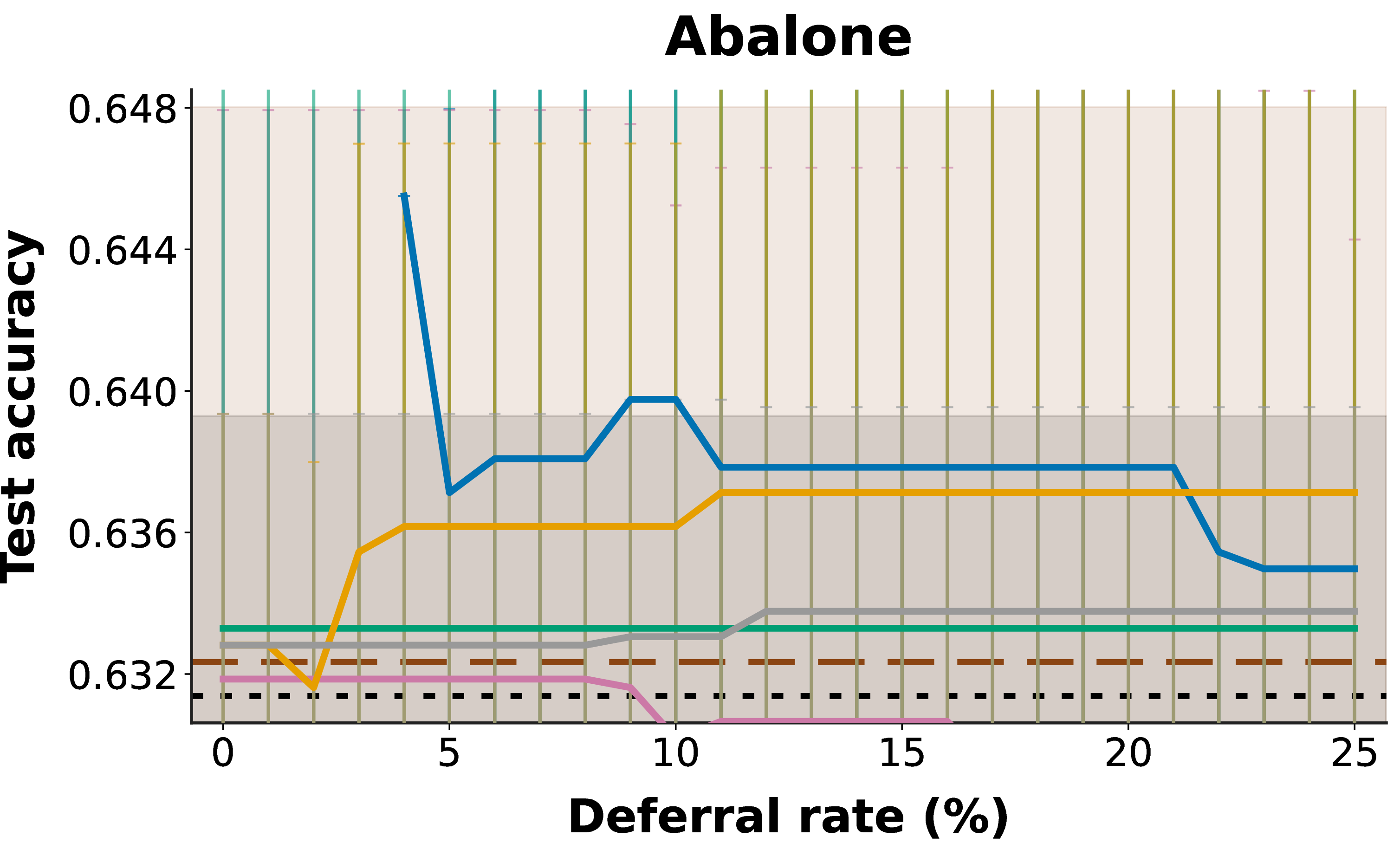

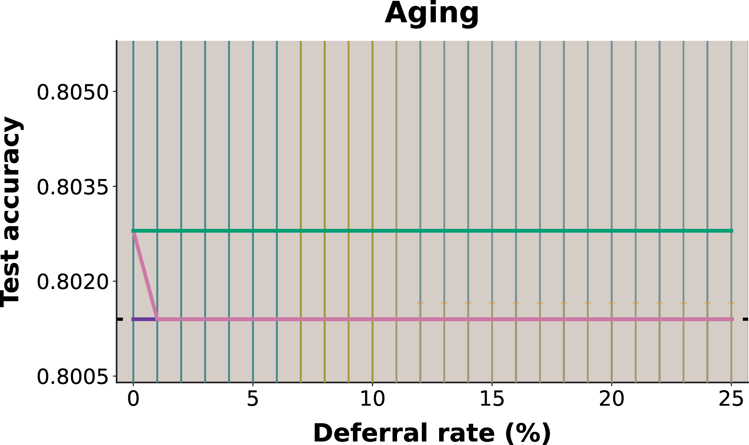
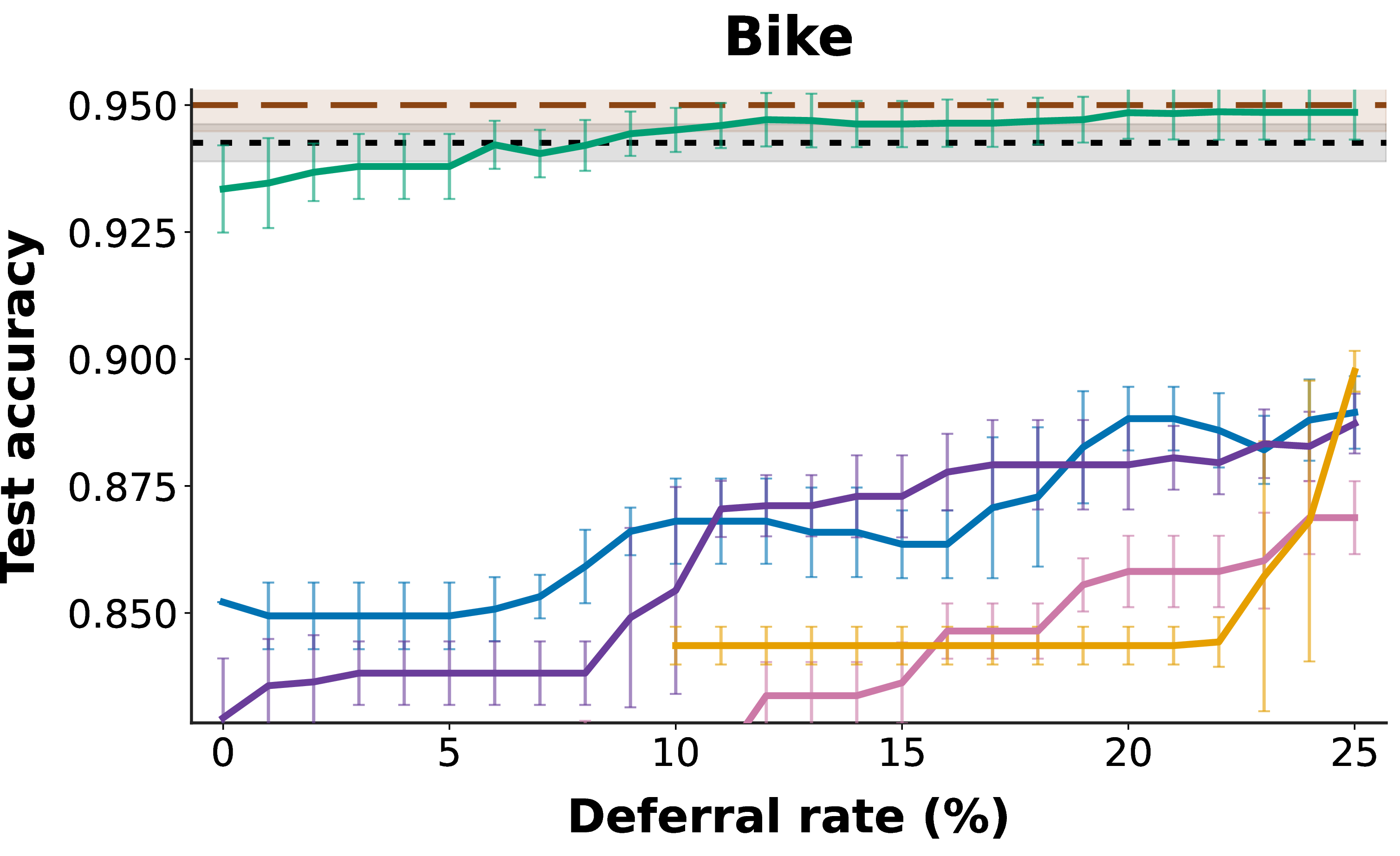


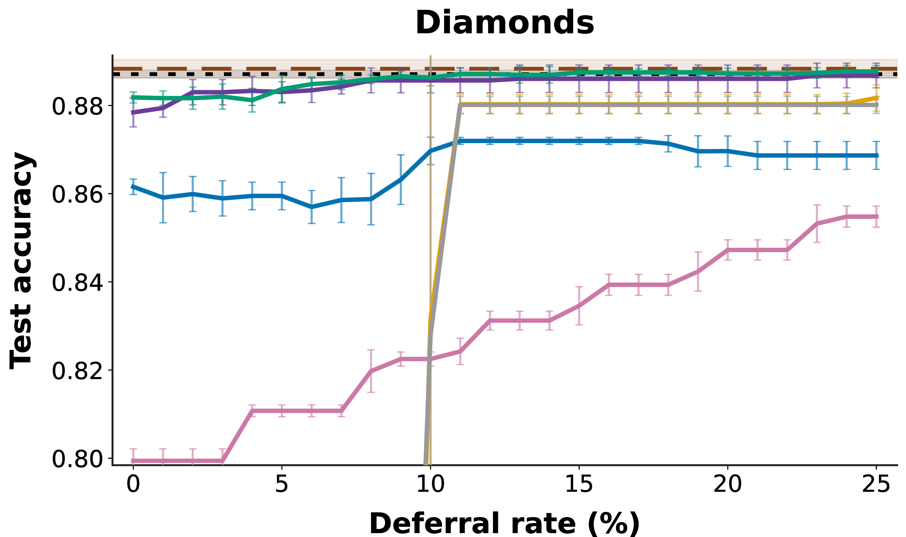
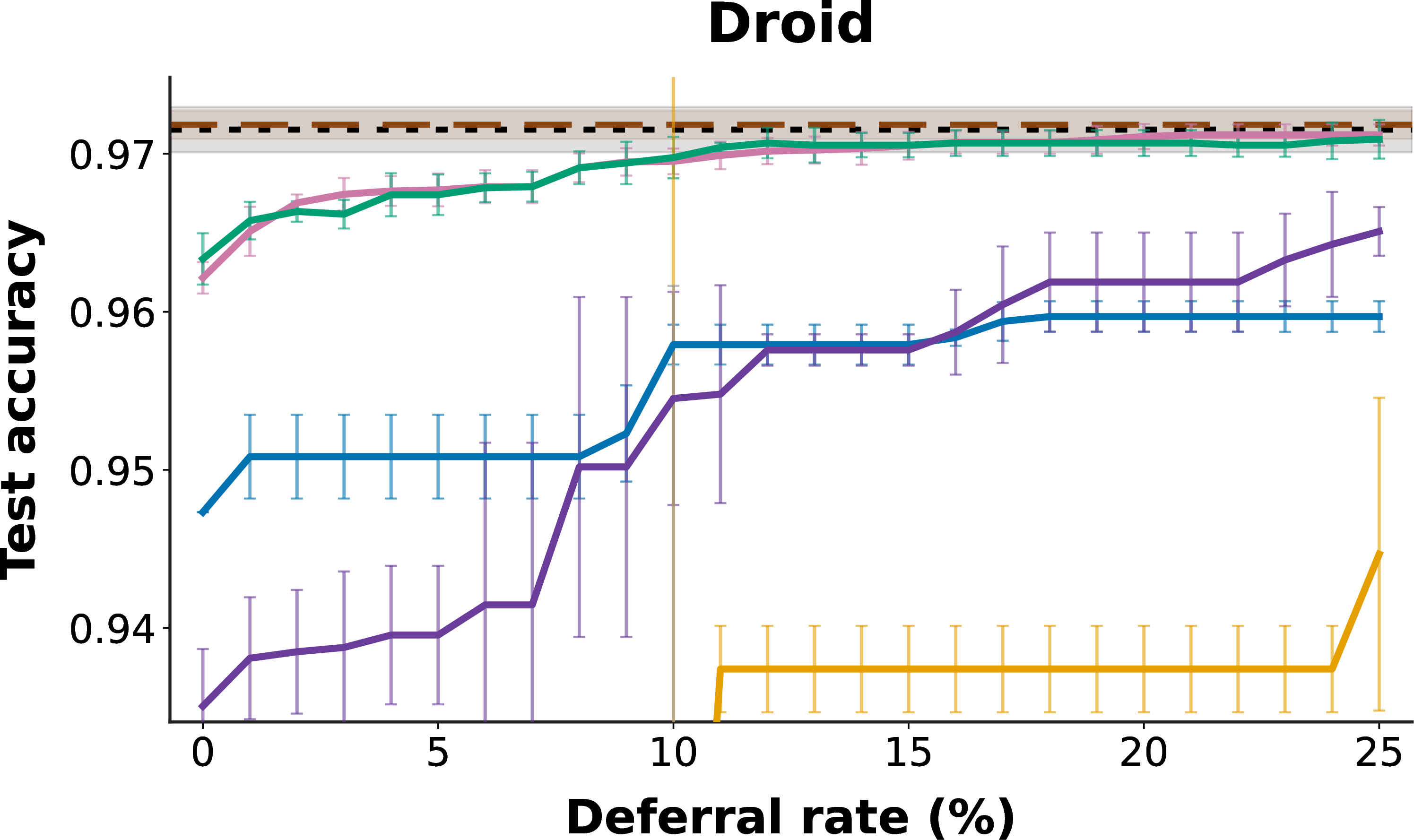
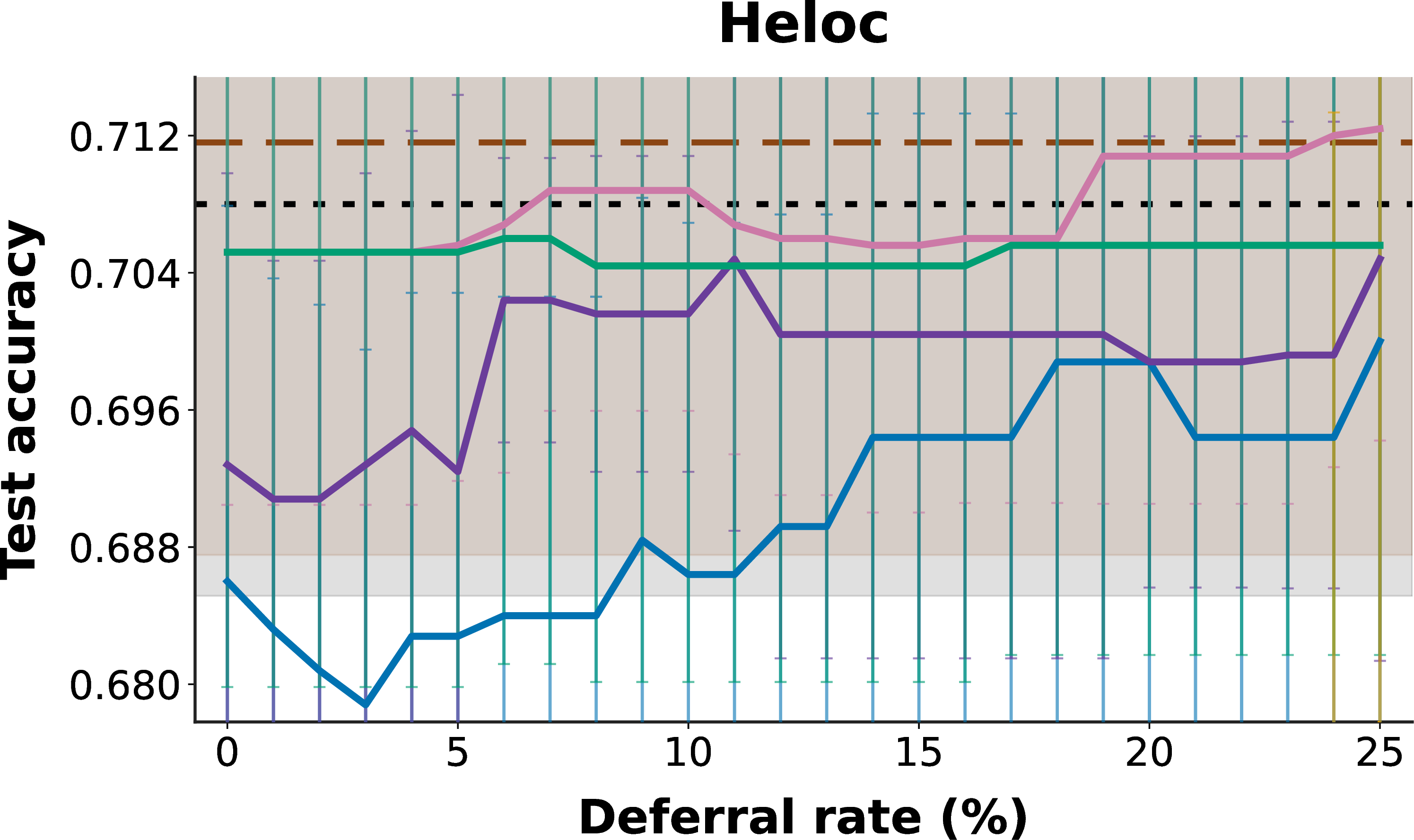
Figure 31: Deferral-accuracy trade-offs for all datasets..
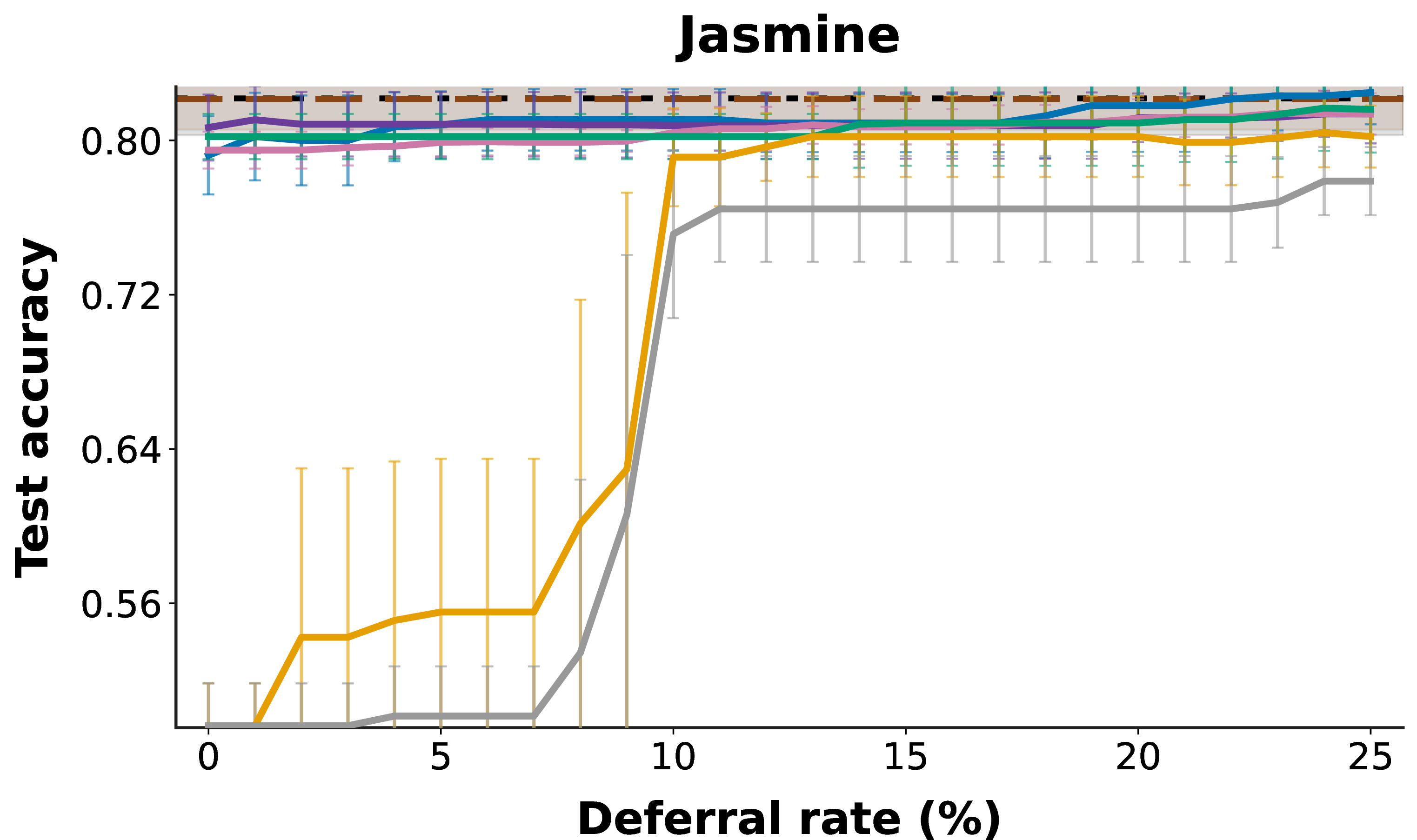
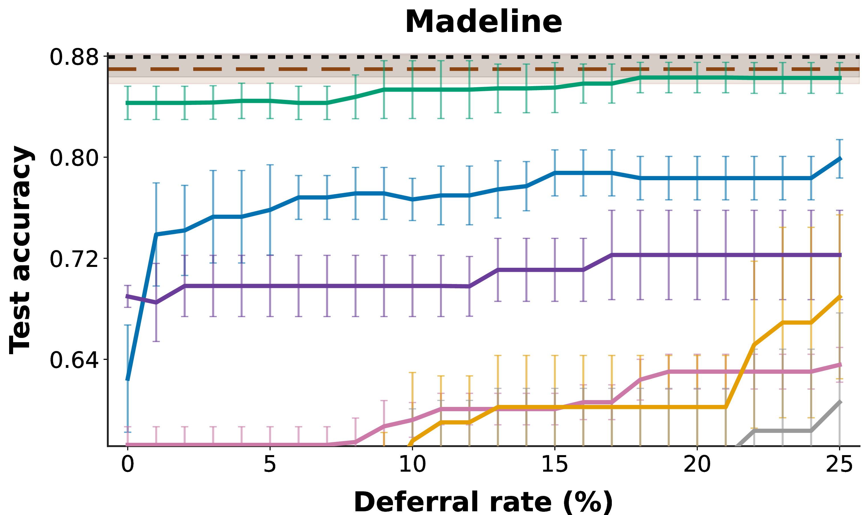
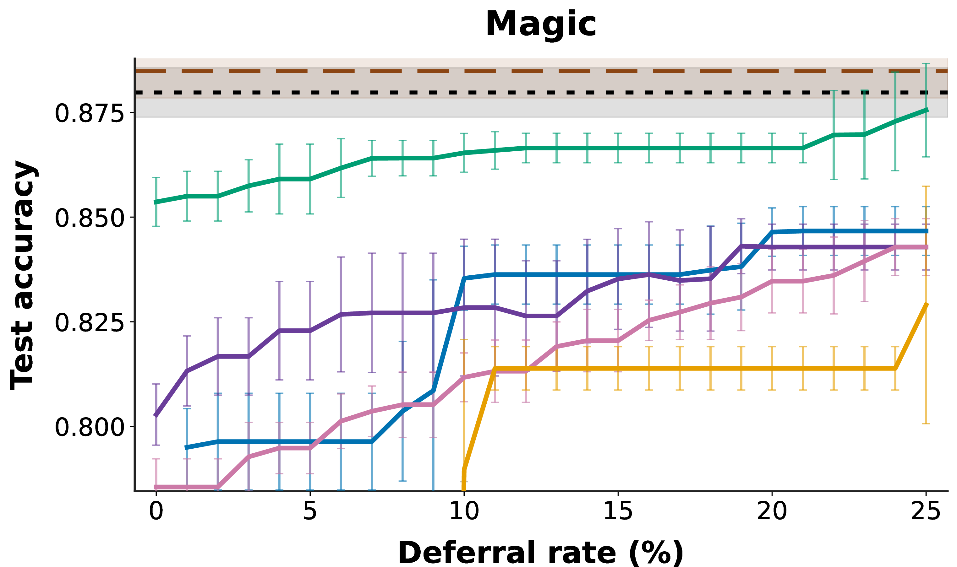
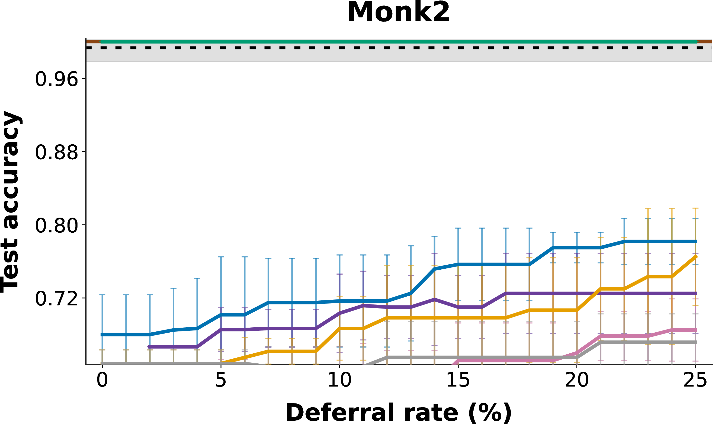
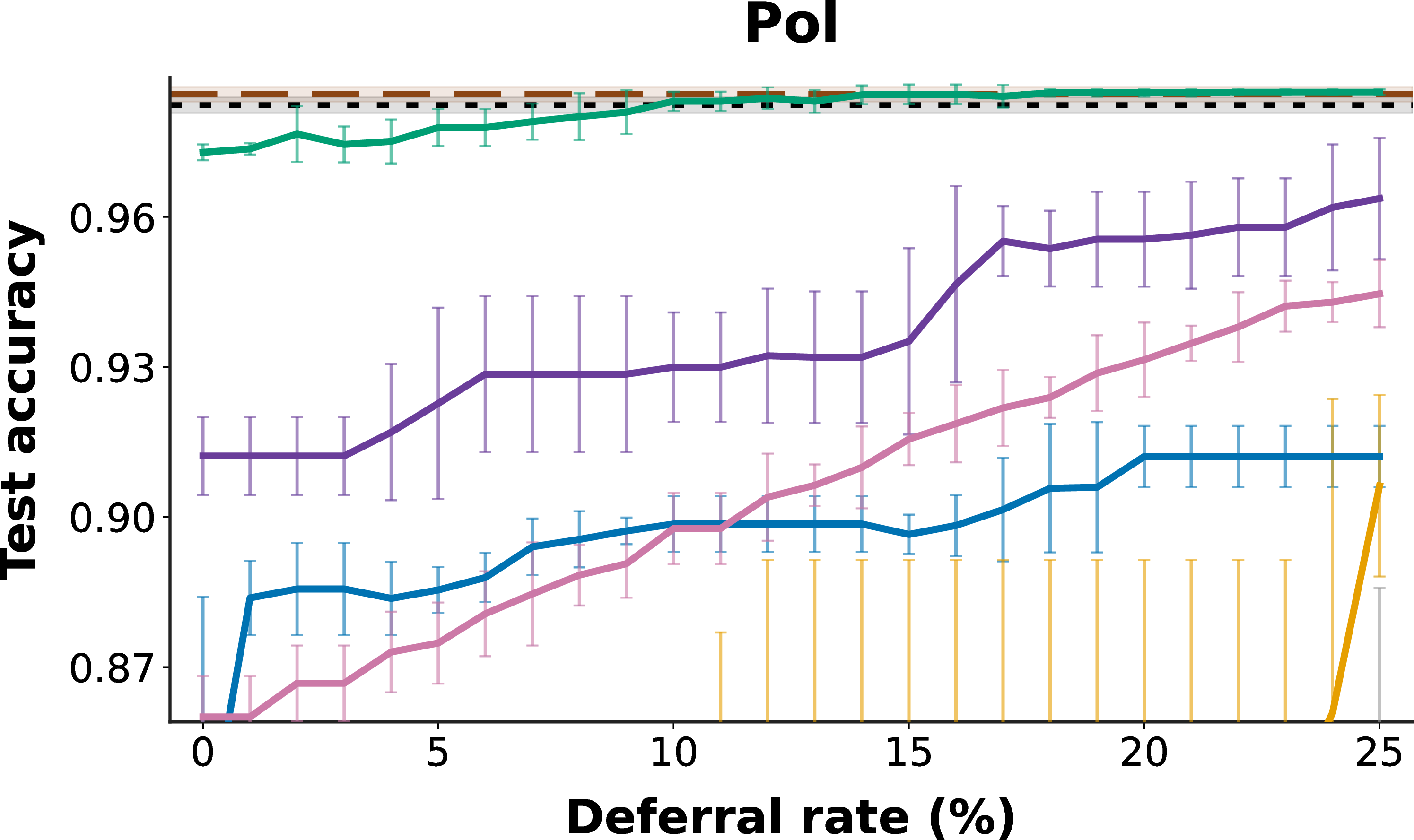
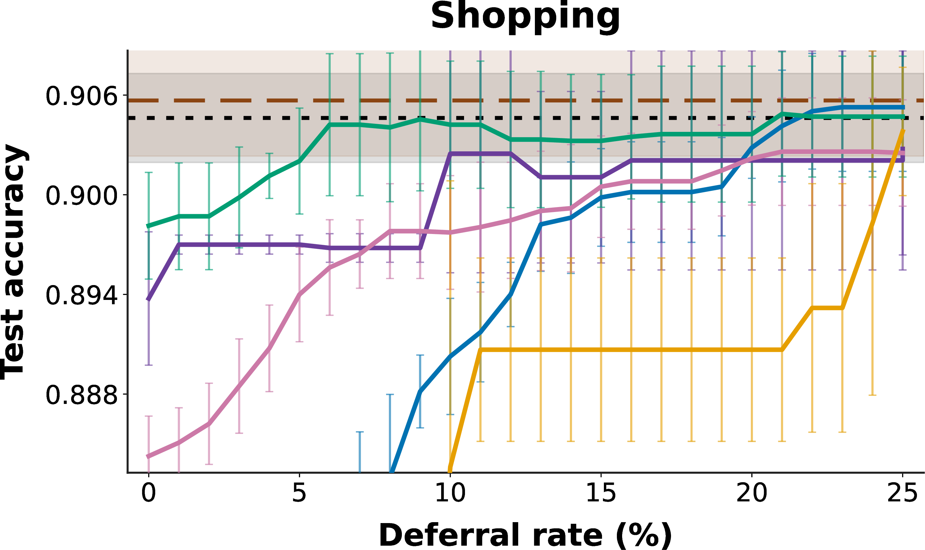
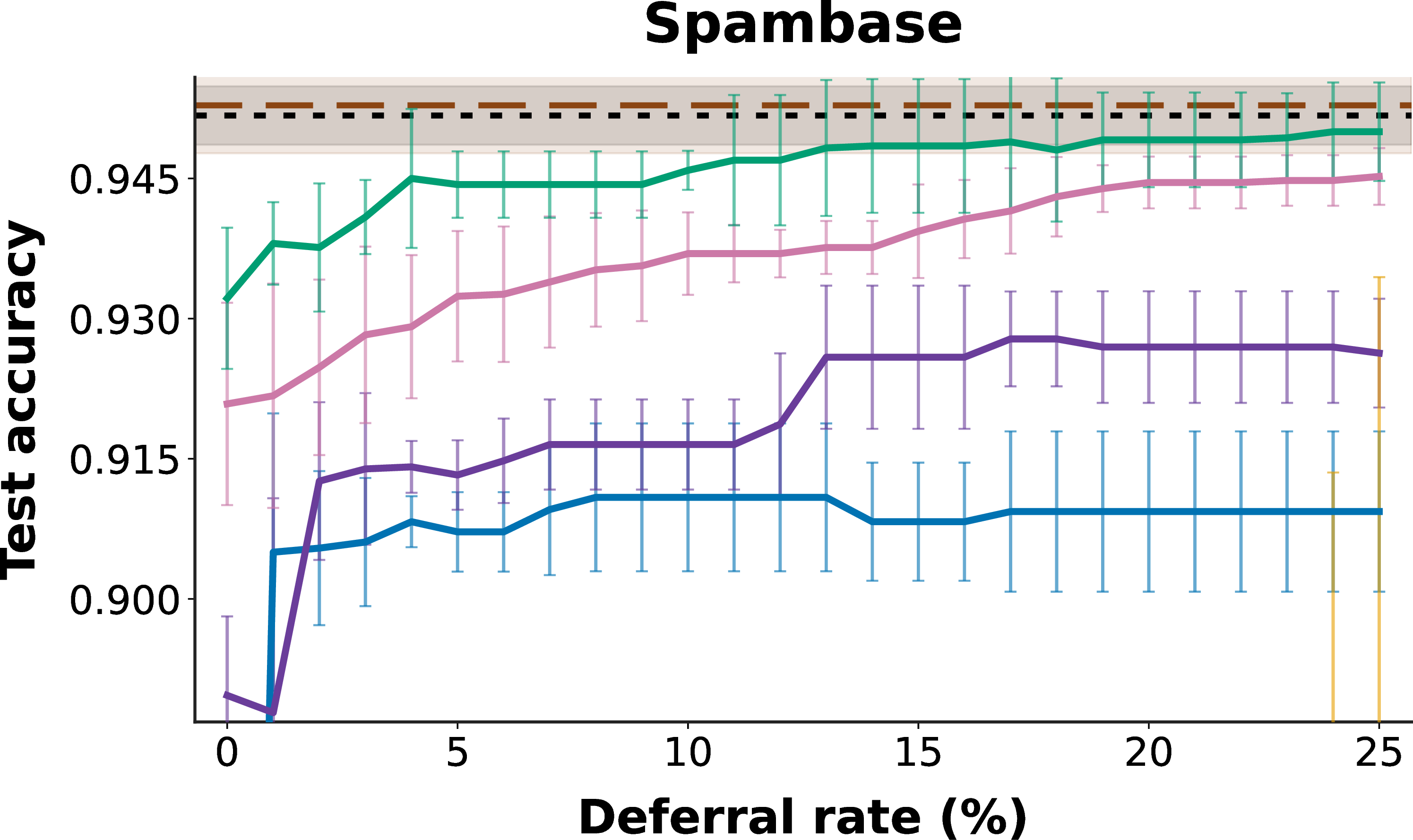
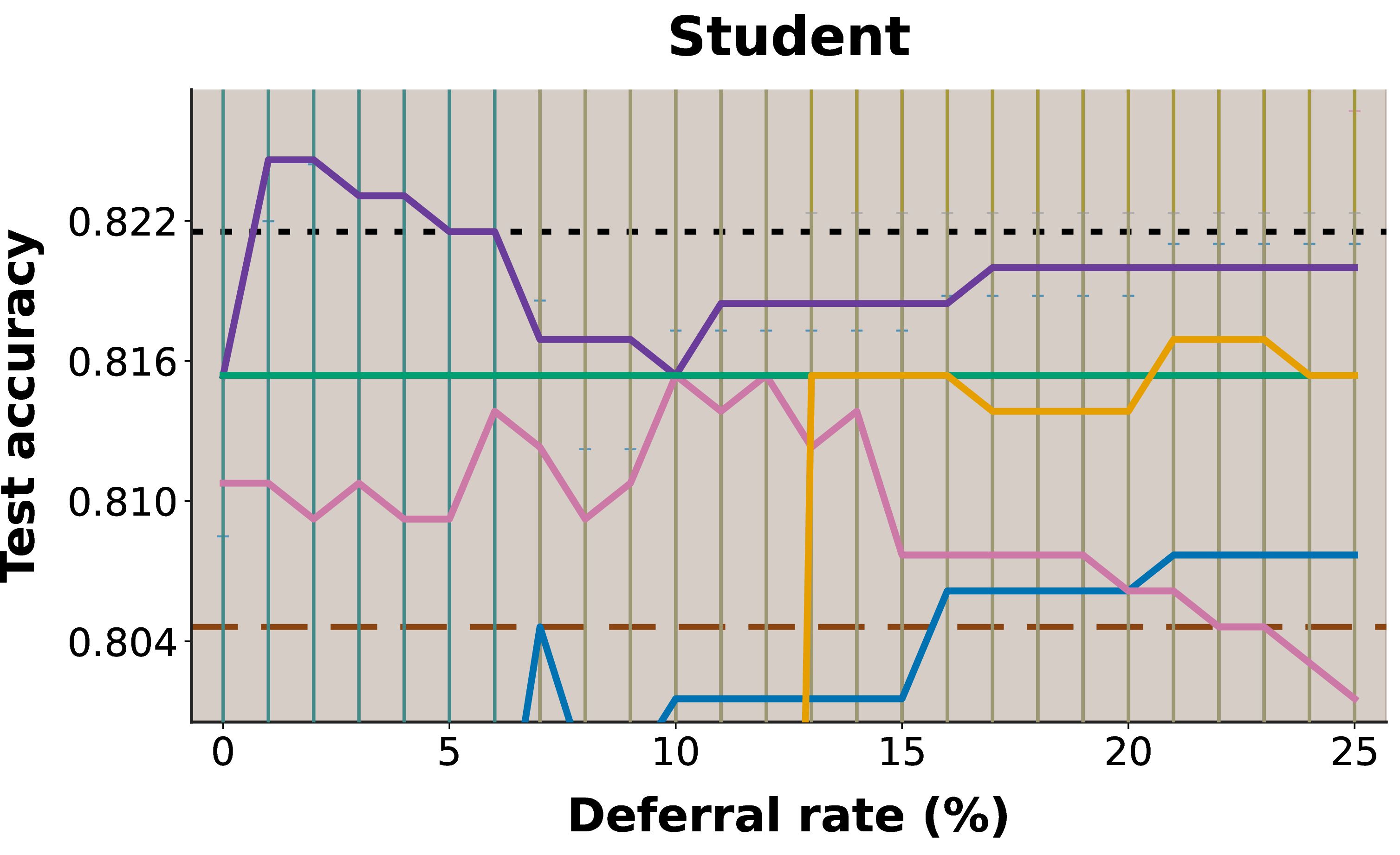
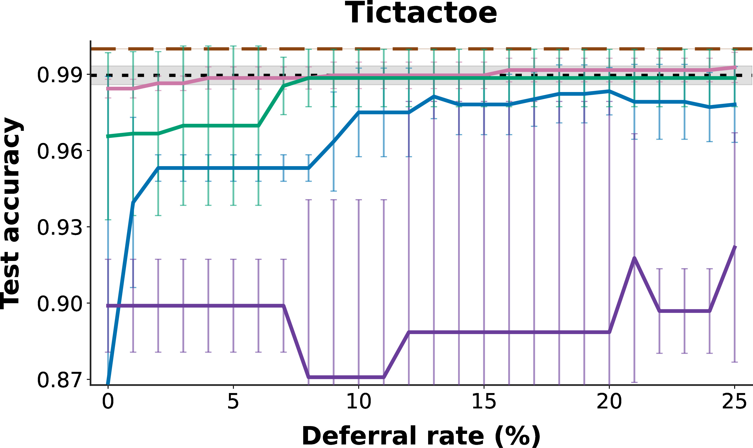
Figure 32: Deferral-accuracy trade-offs for all datasets, continued..
13.1 Ablations↩︎
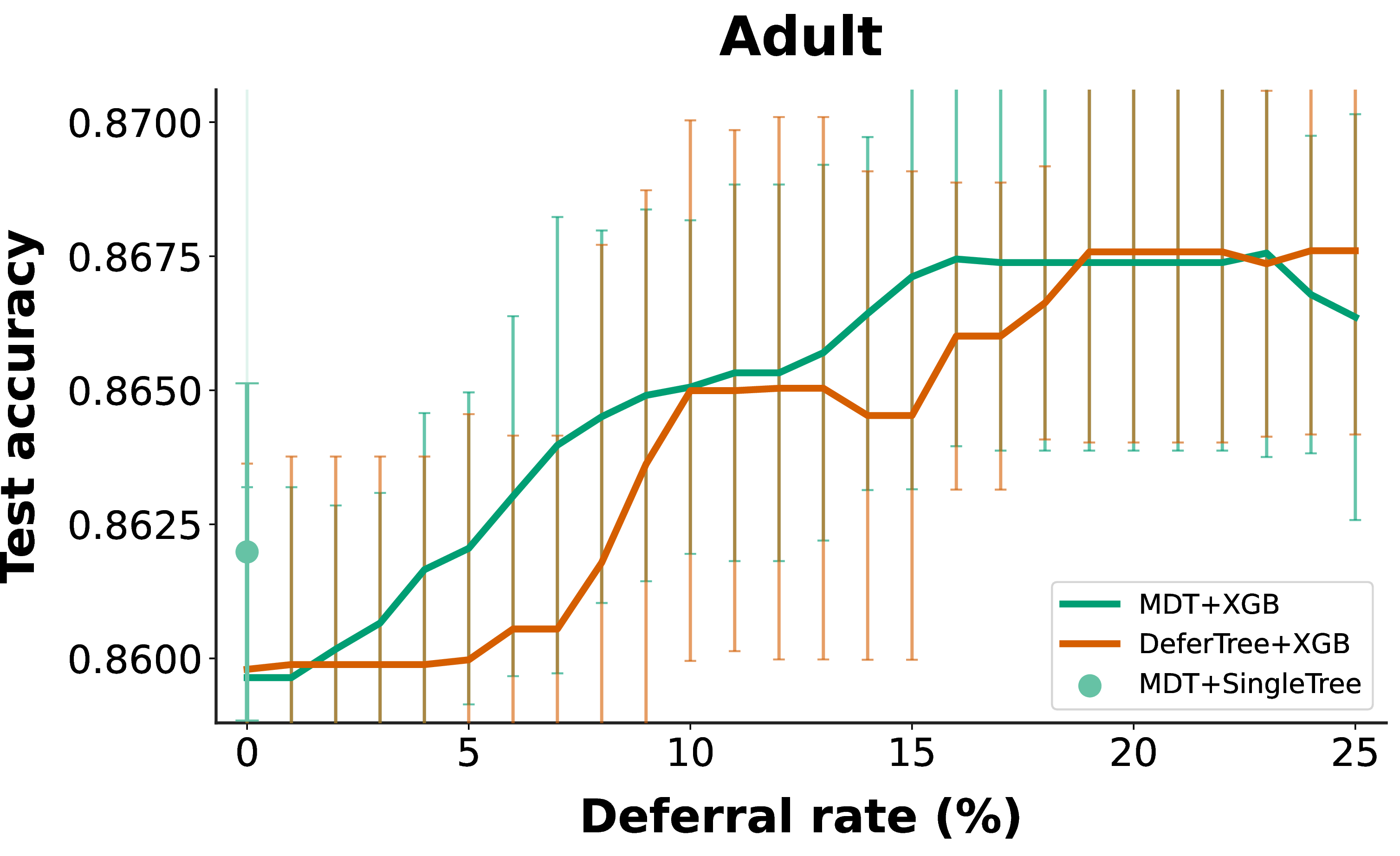
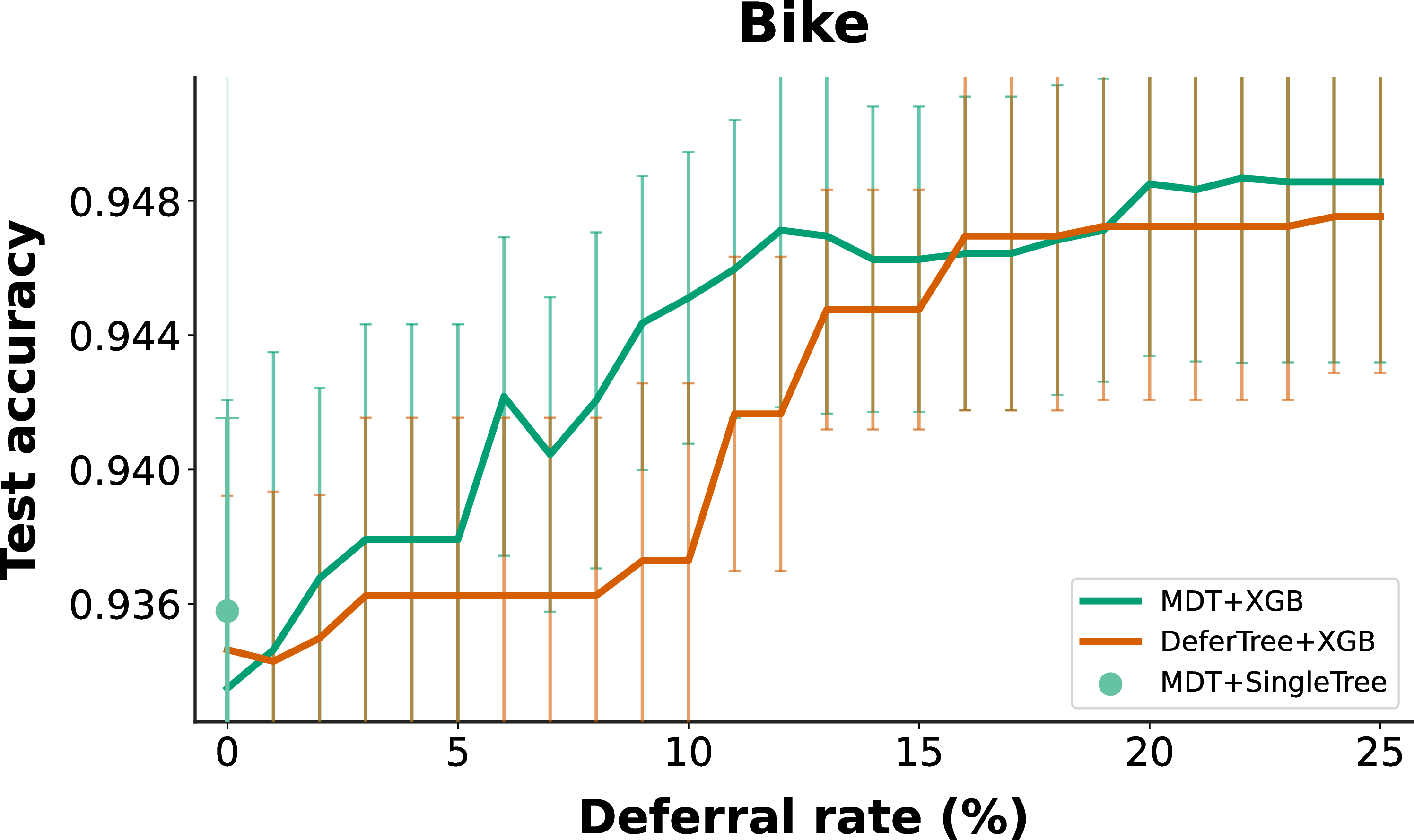


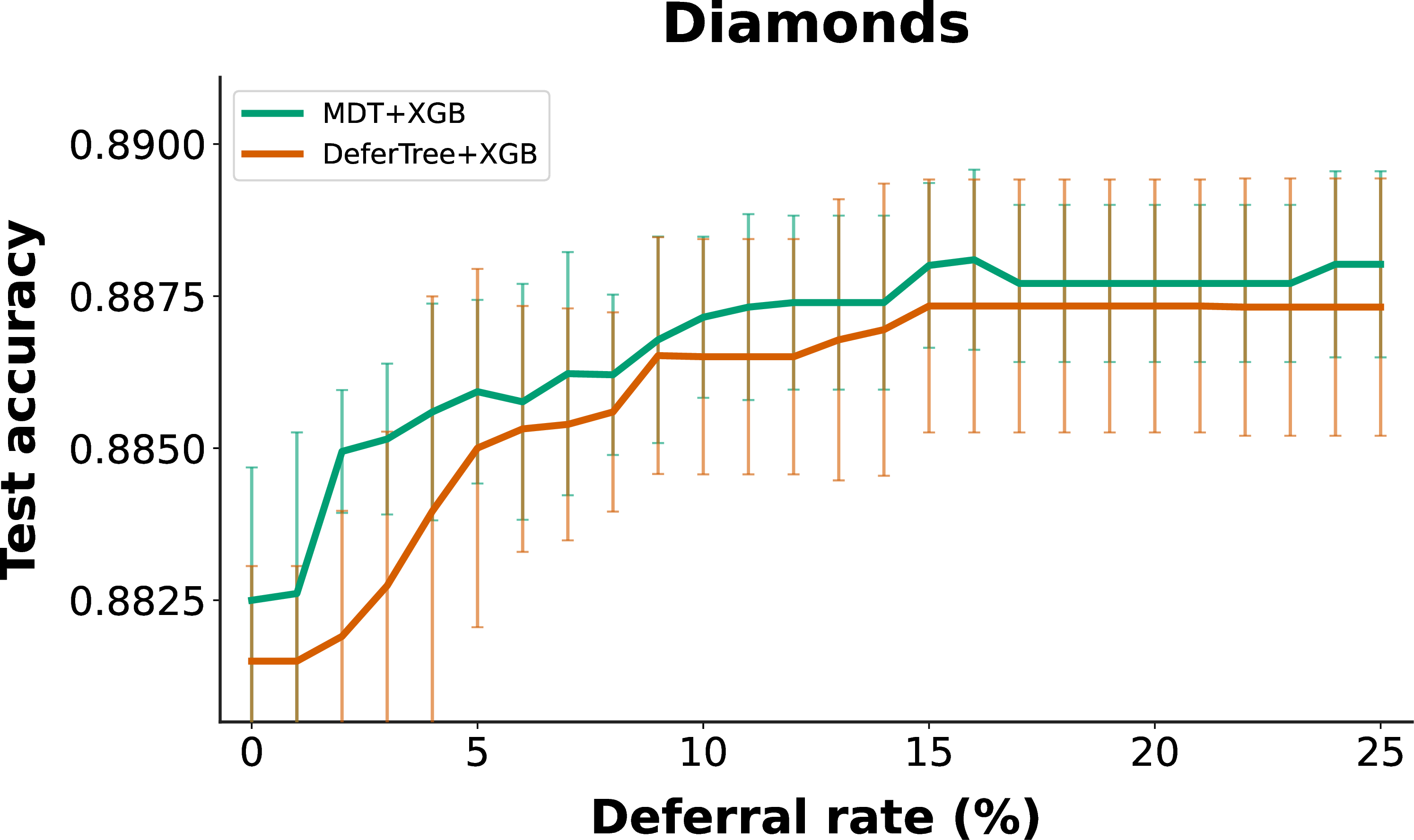
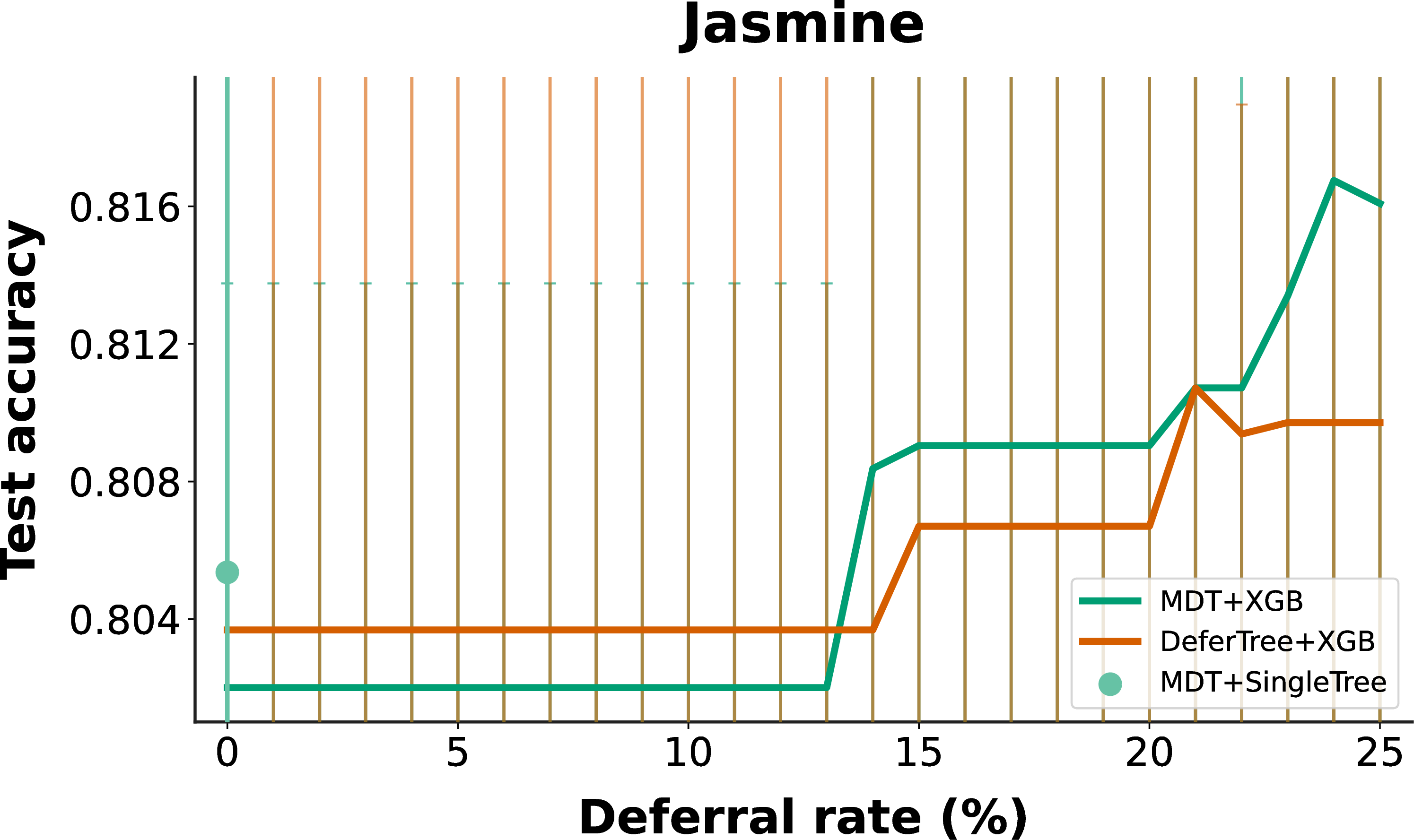
Figure 33: Results of our MDT algorithm compared to just using our DeferTree algorithm. Here, we also show results for MDT+SingleTree, which uses a single decision tree algorithm as fallback instead of XGBoost. When the deferral rate is 0, DeferTree+XGB turns into a near-optimal decision tree algorithm. We see that MDT+SingleTree is able to provide a much better, fully interpretable model than a near-optimal tree in most cases..
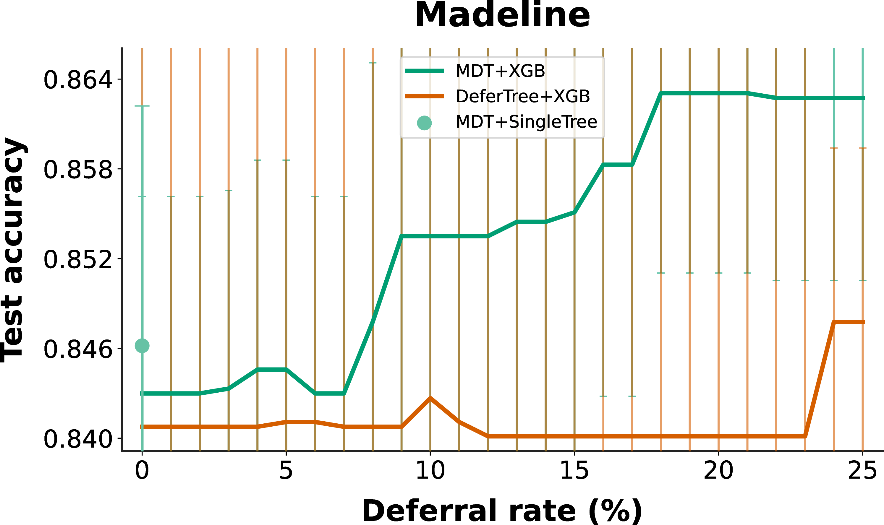
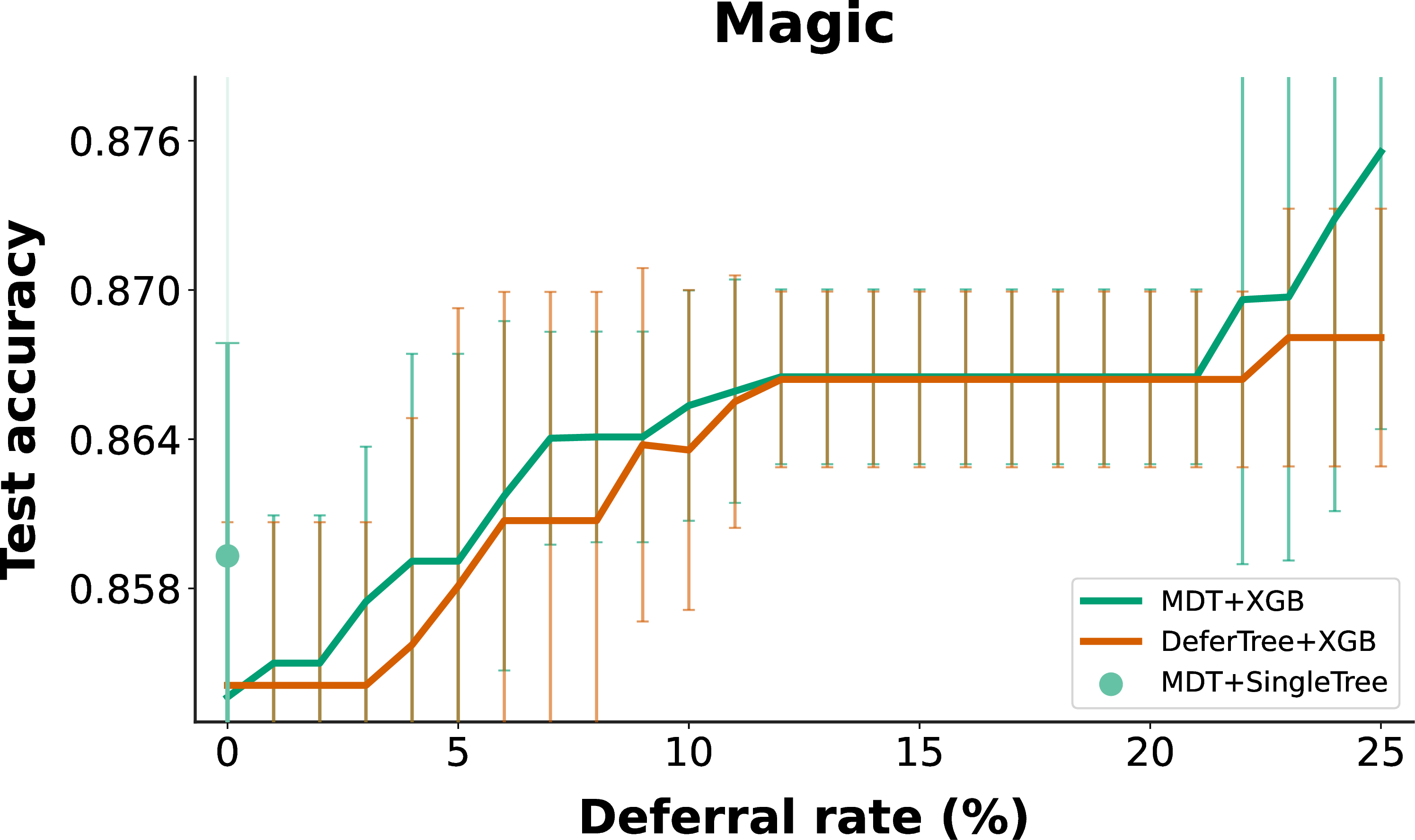
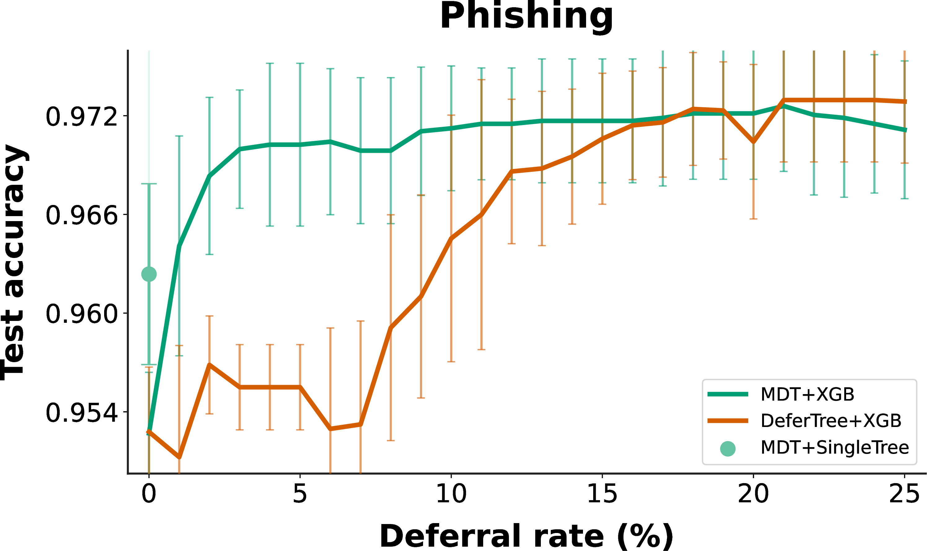
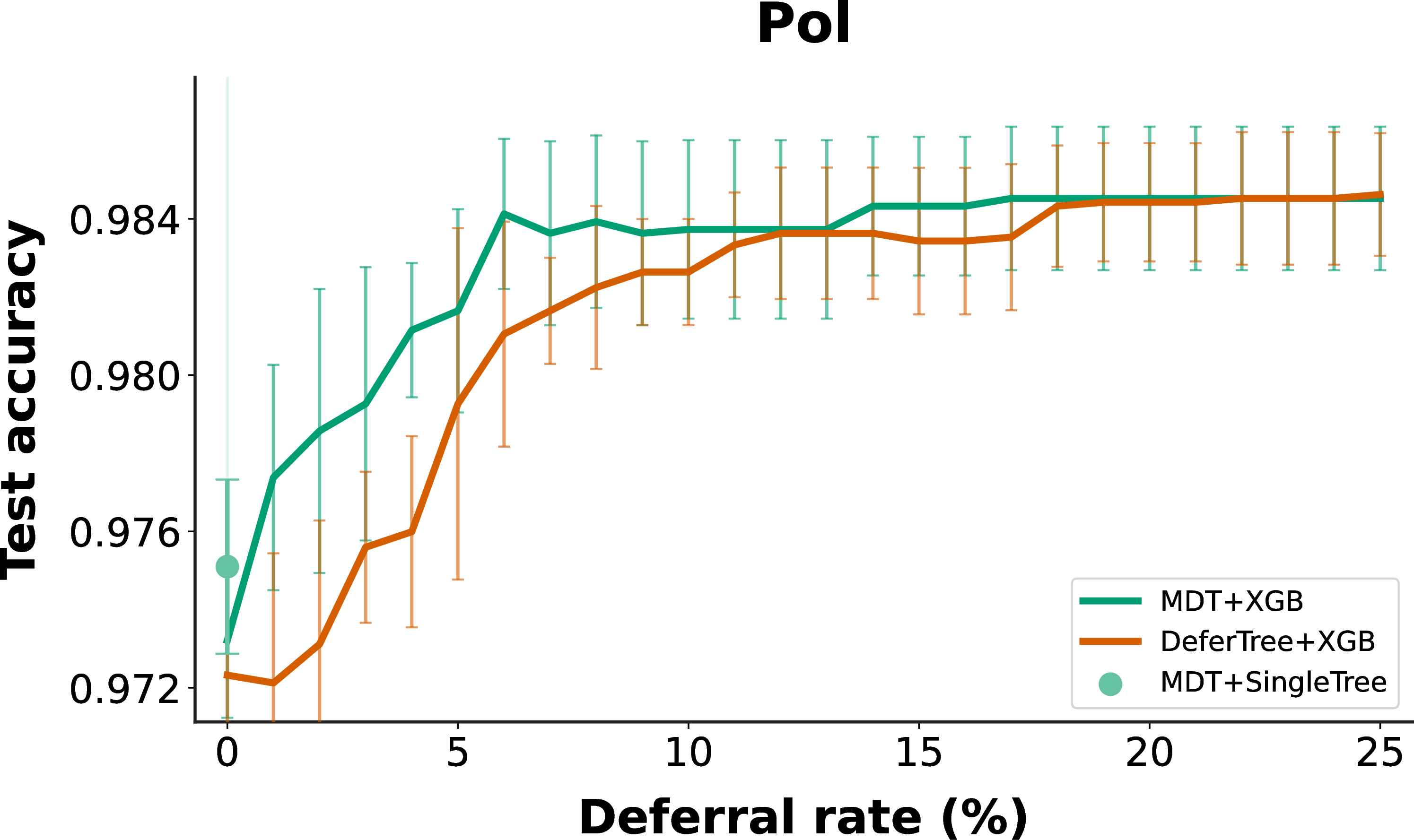

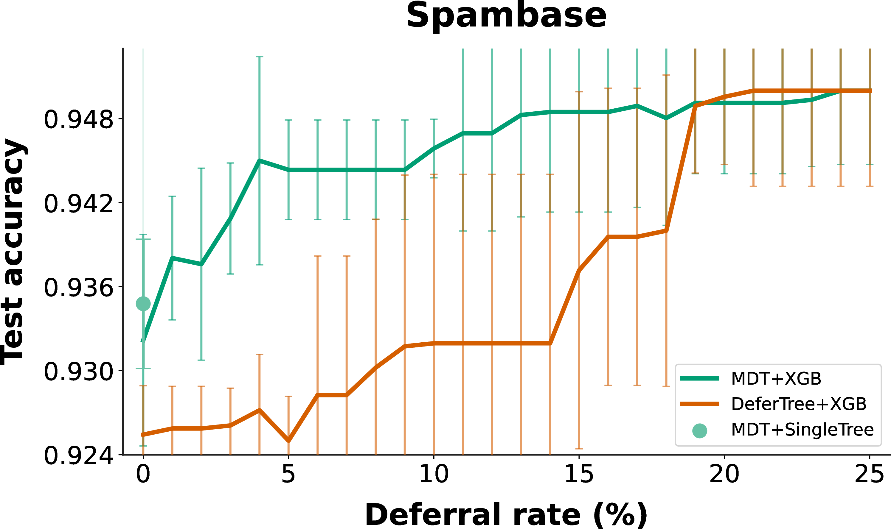
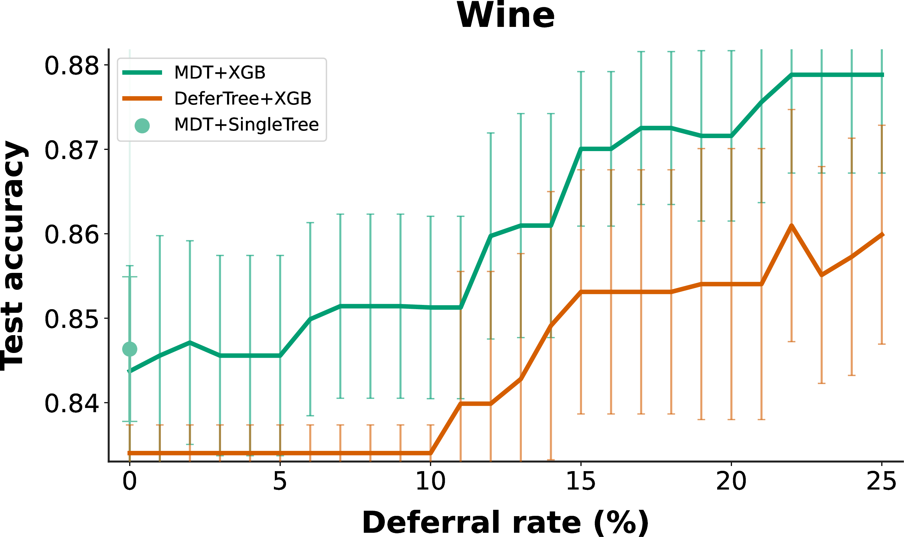
Figure 34: Results of our MDT algorithm compared to just using our DeferTree algorithm (continued)..

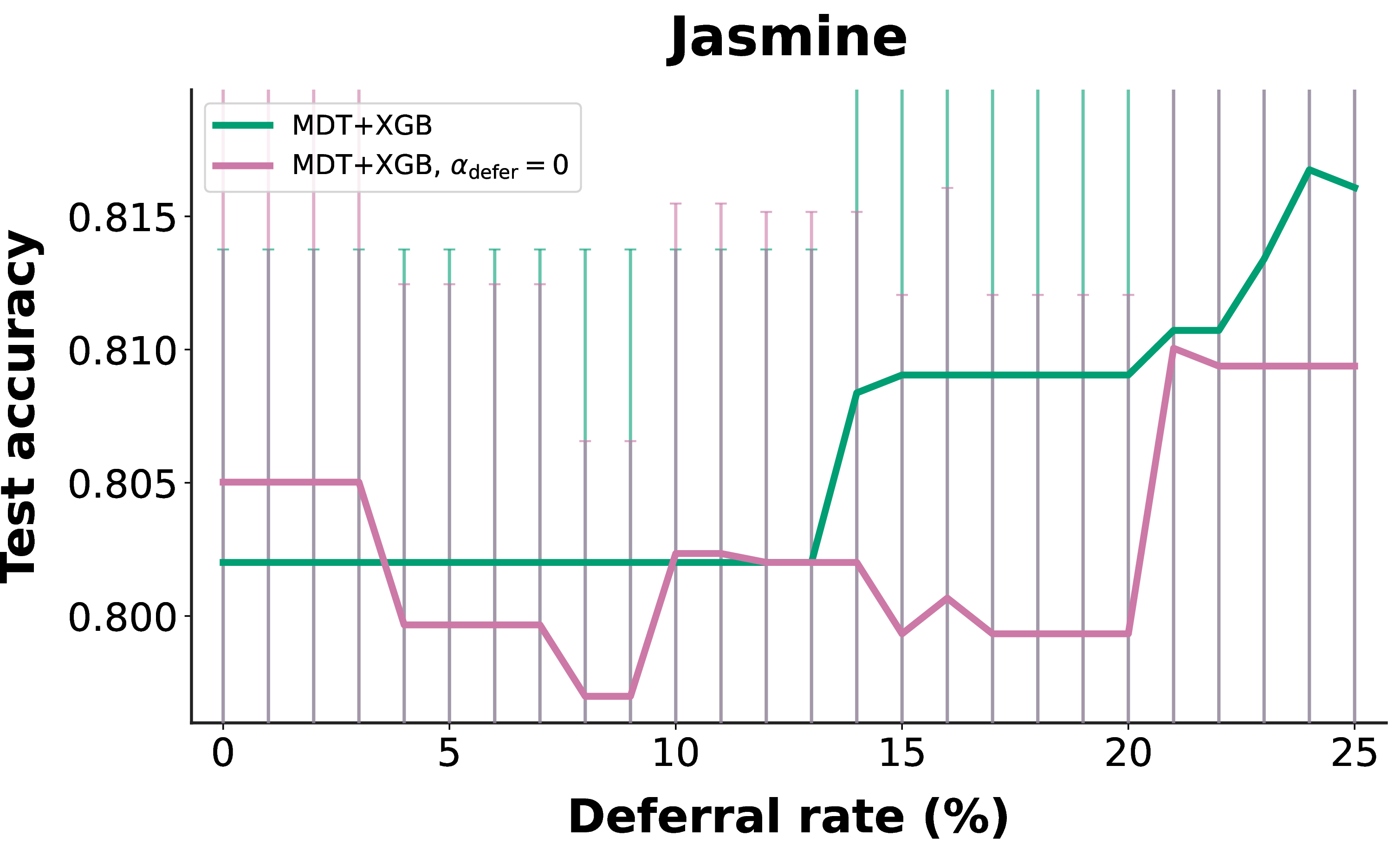
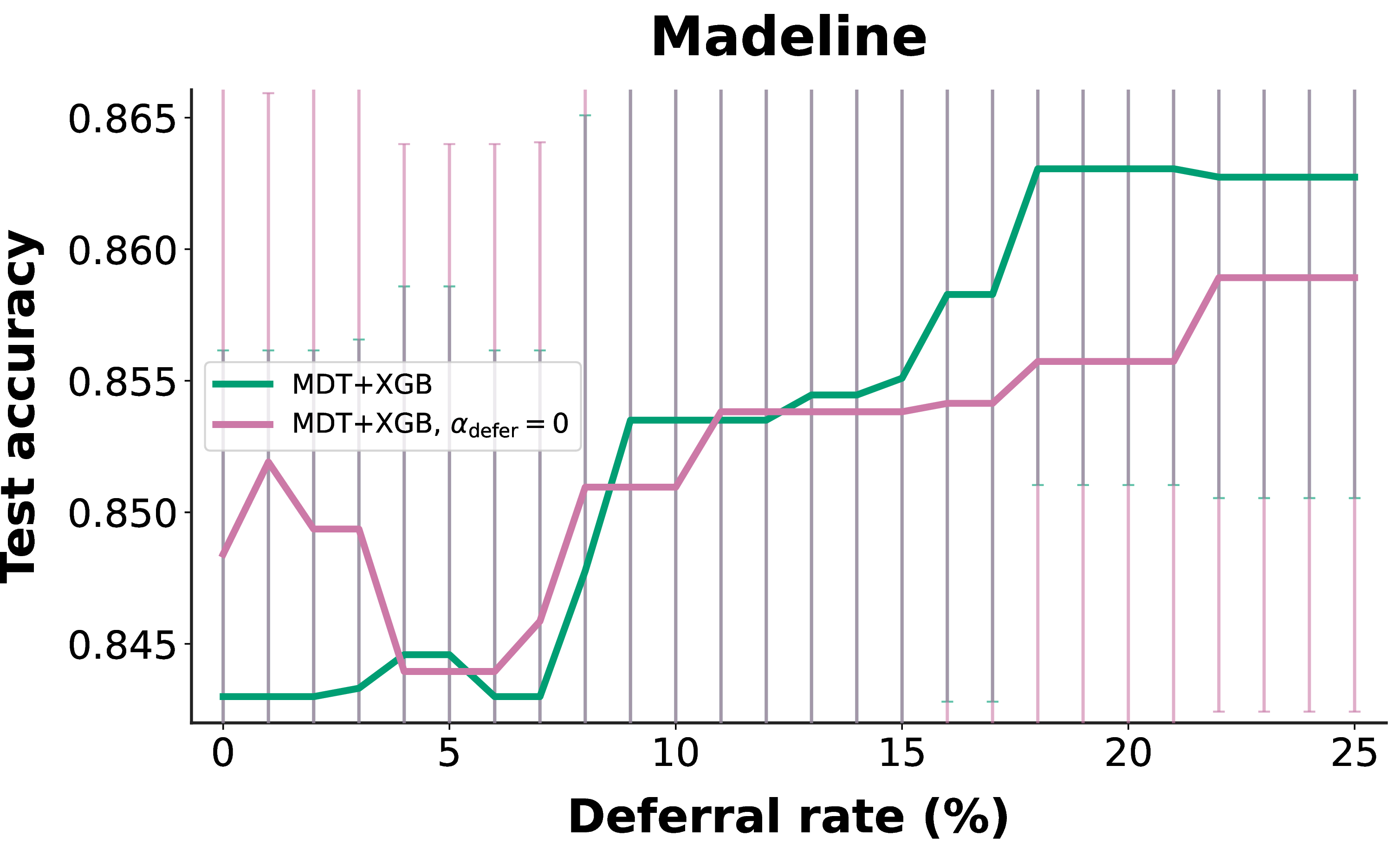
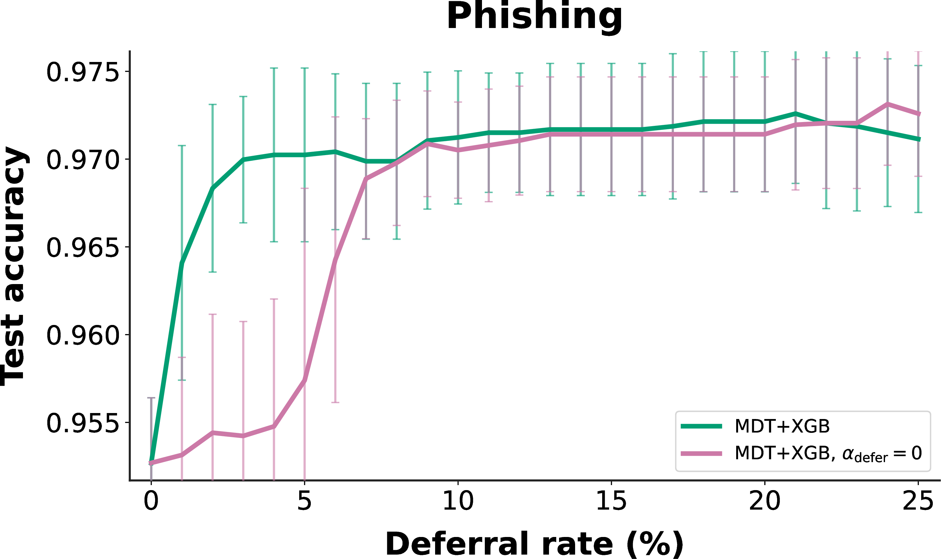
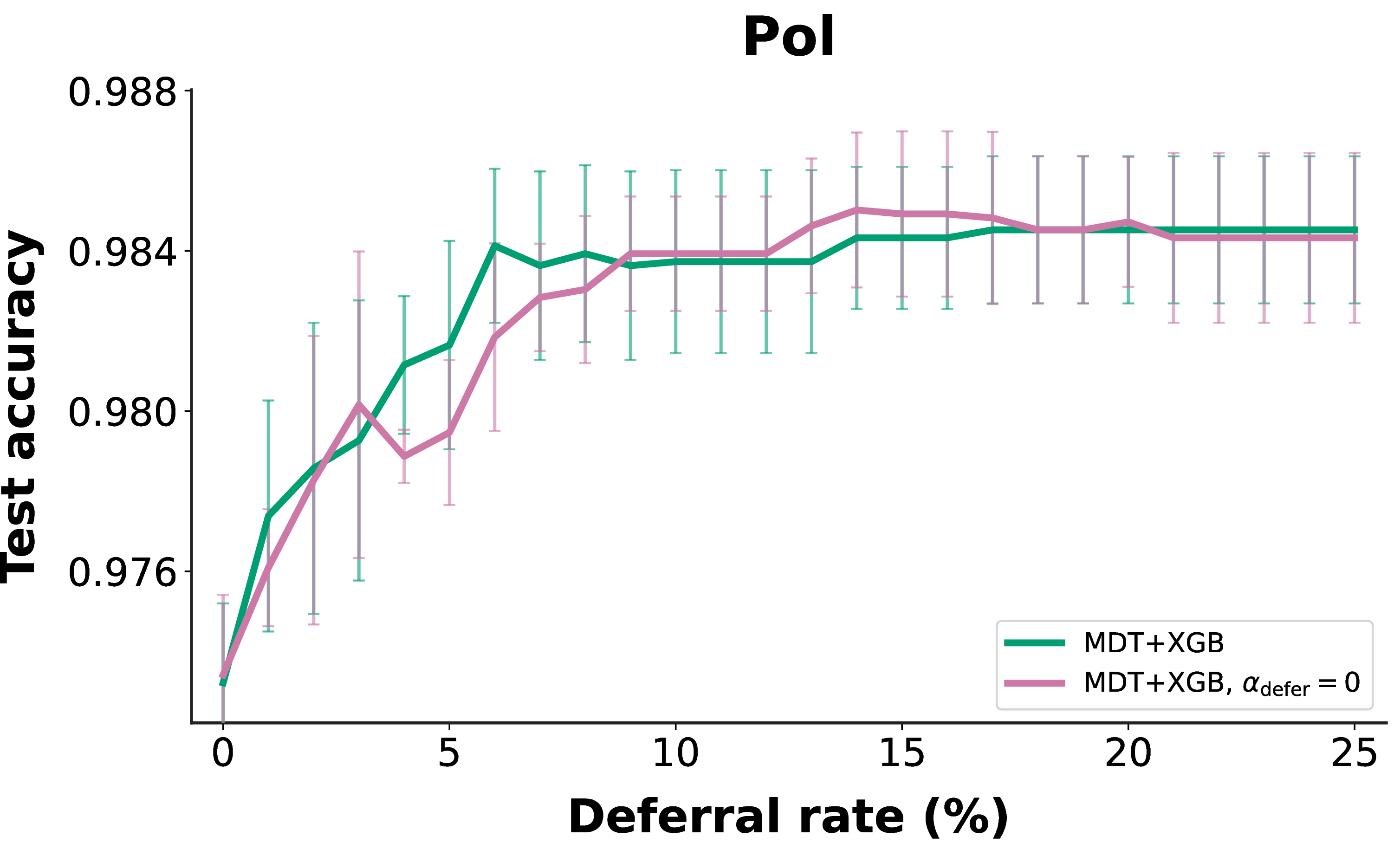
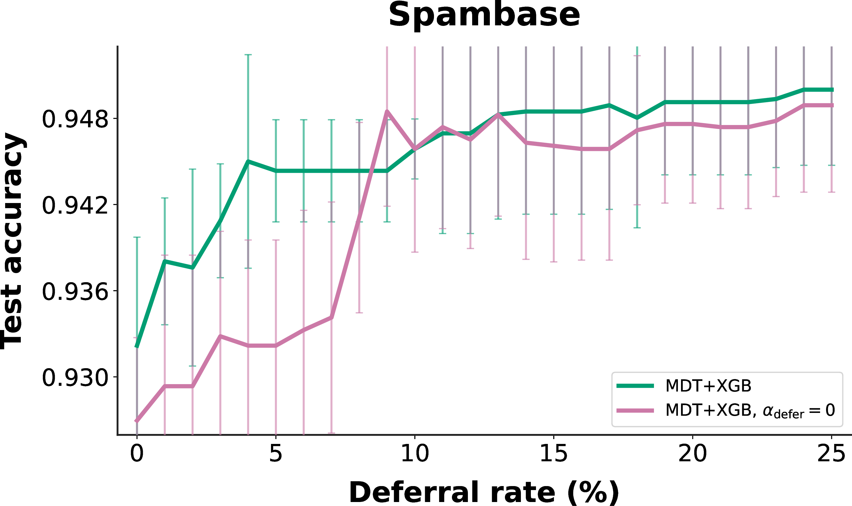
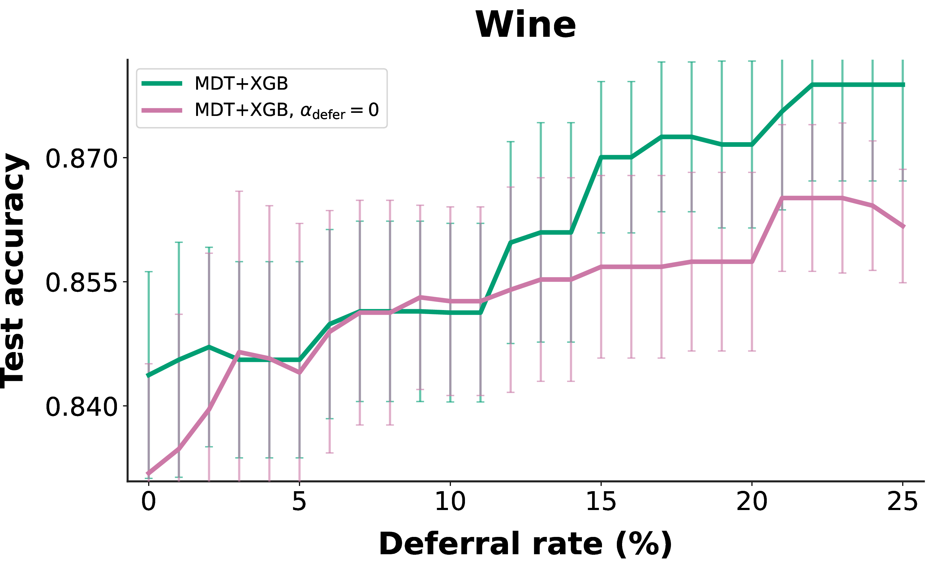
Figure 35: Ablation on the impacts of rescaling \(\tau\) for later stages of the MDT. The boolean \(\texttt{rescale\_tau}\) is set to 0 for the \(\alpha_{\text{defer}}=0\) method..

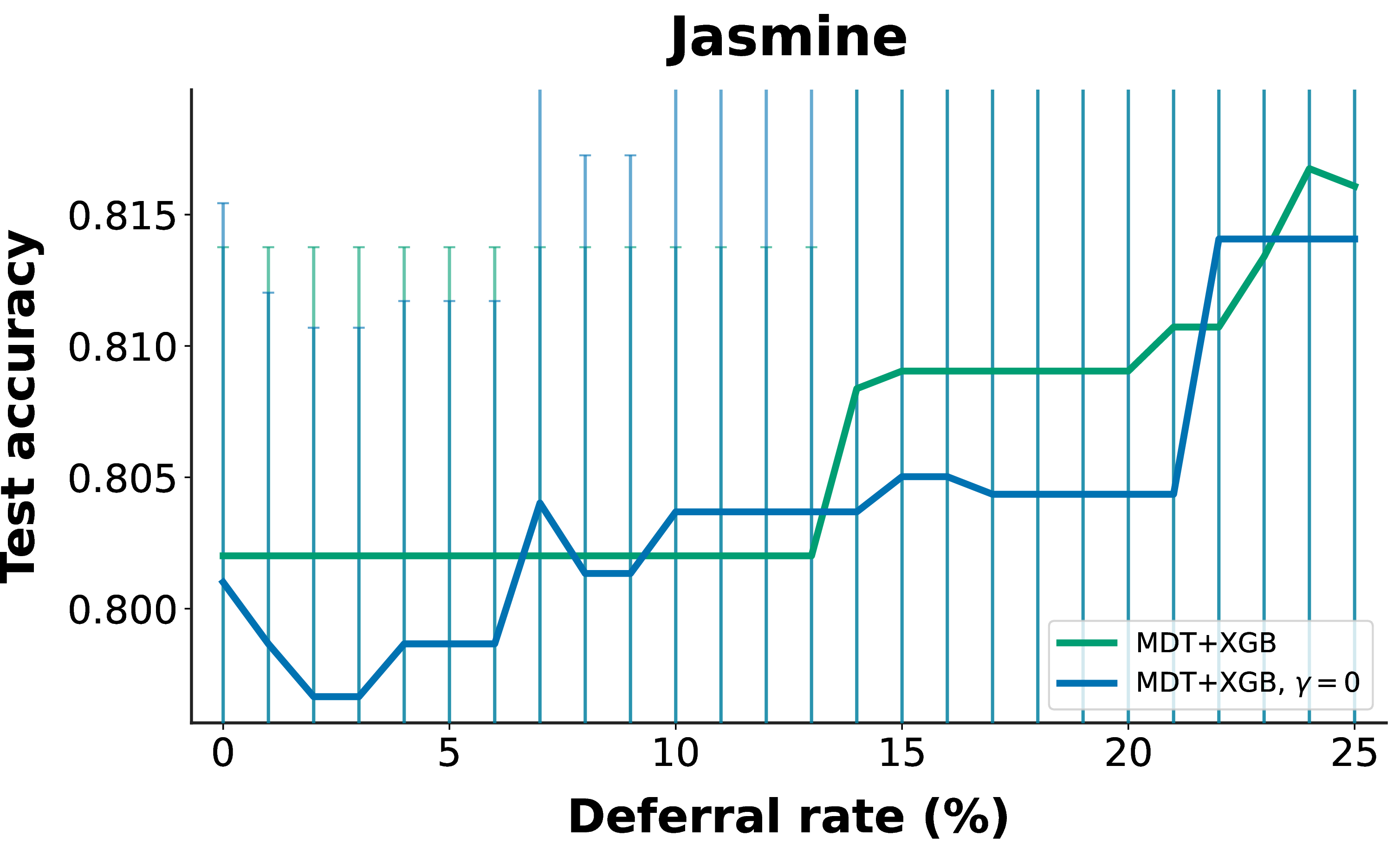
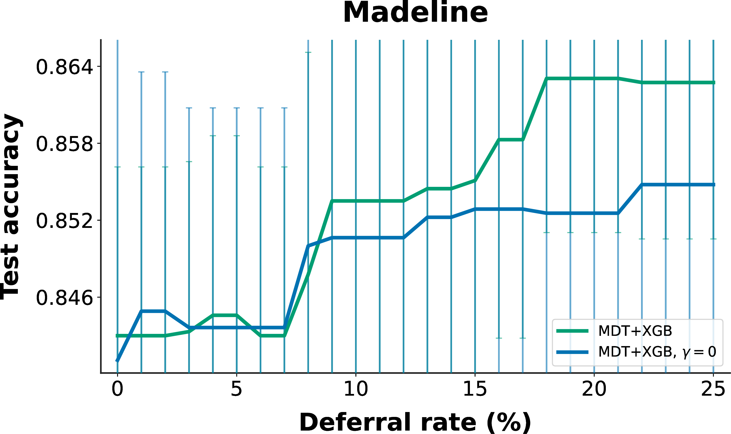
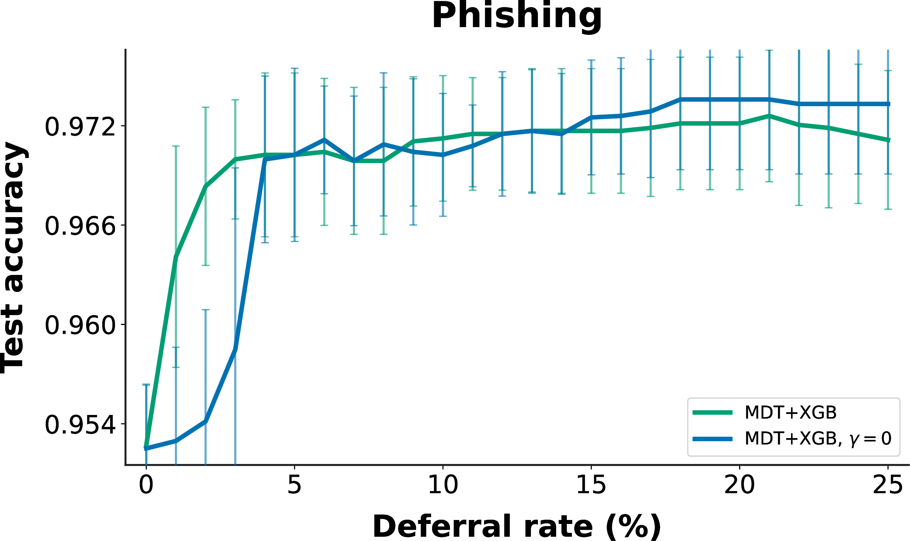
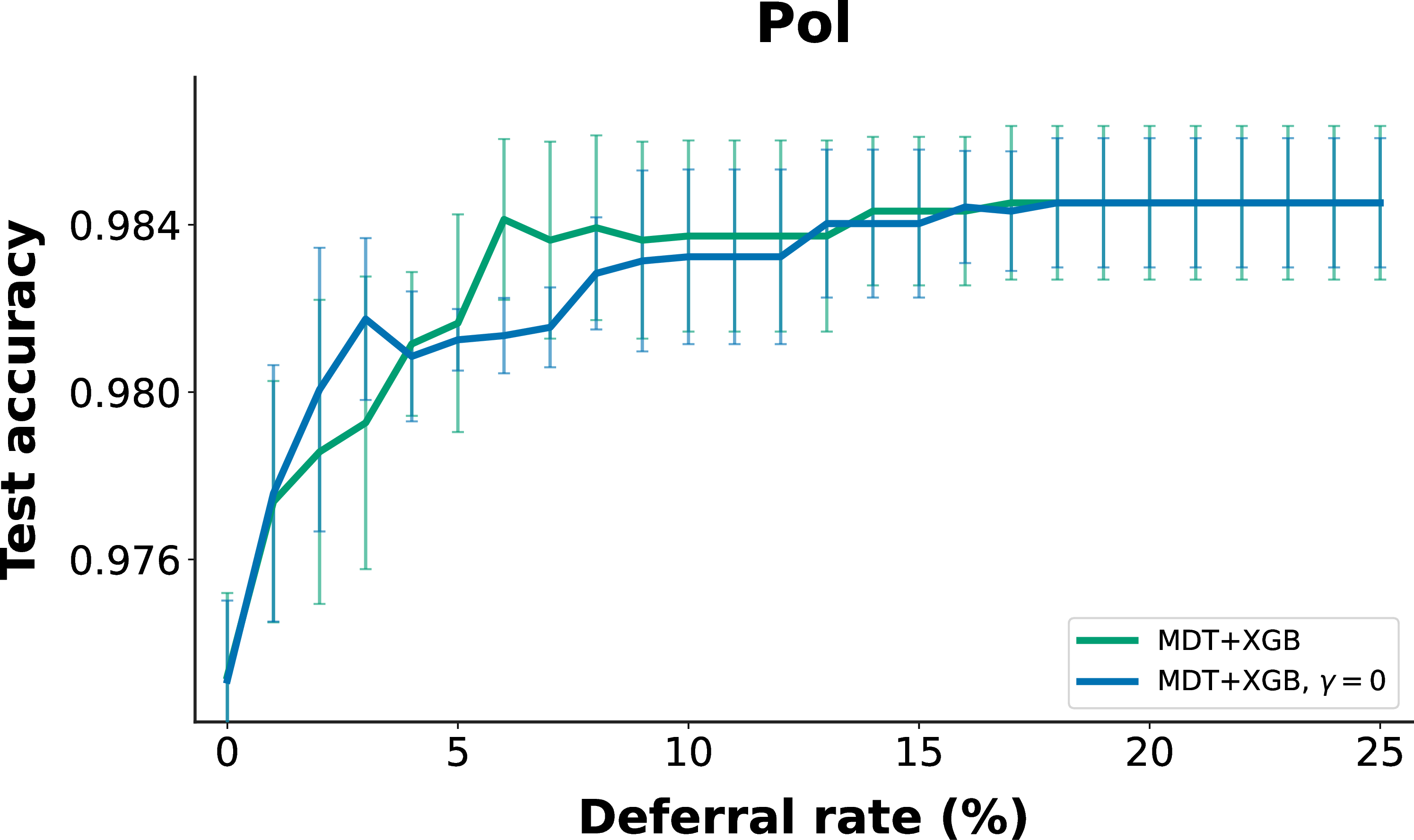
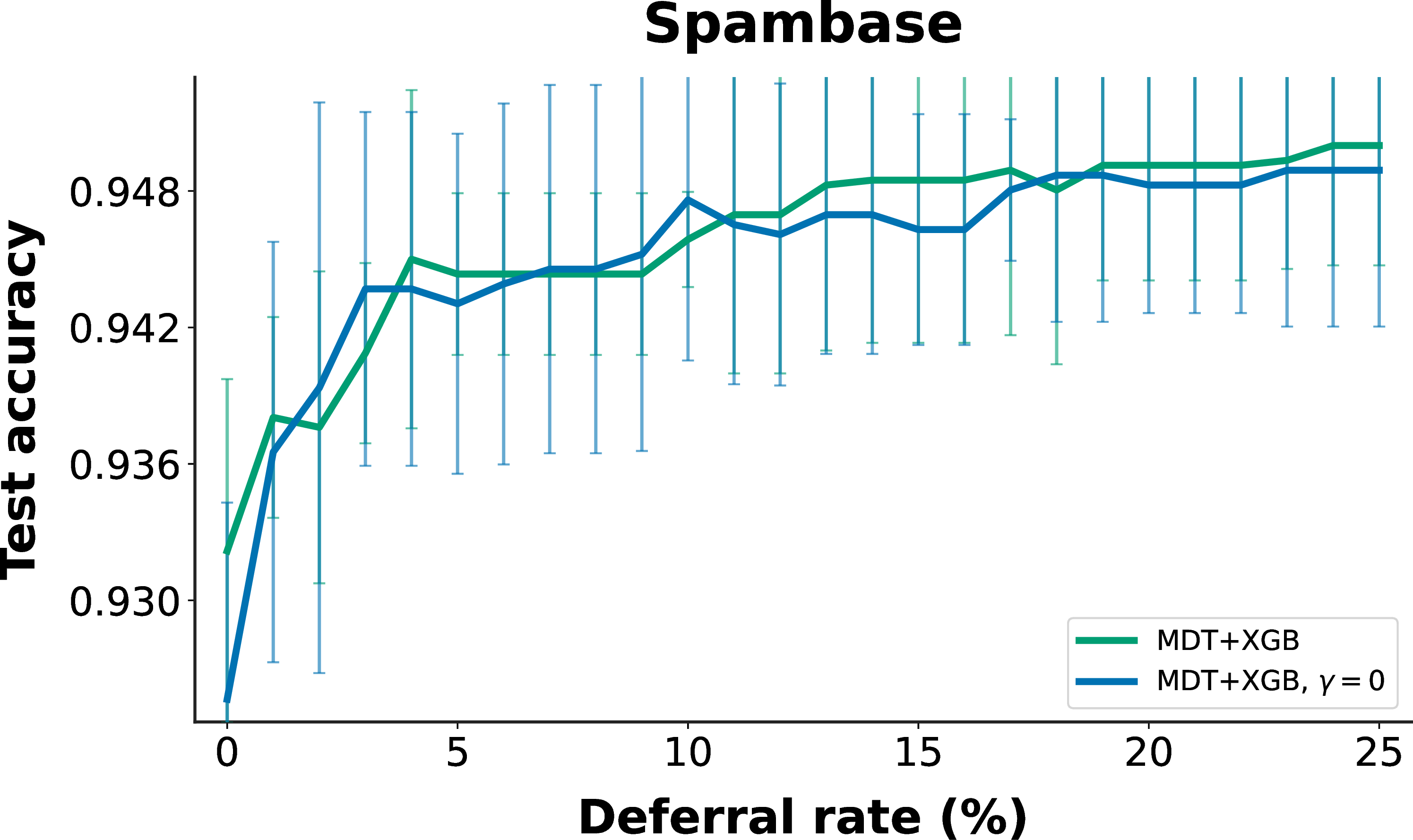
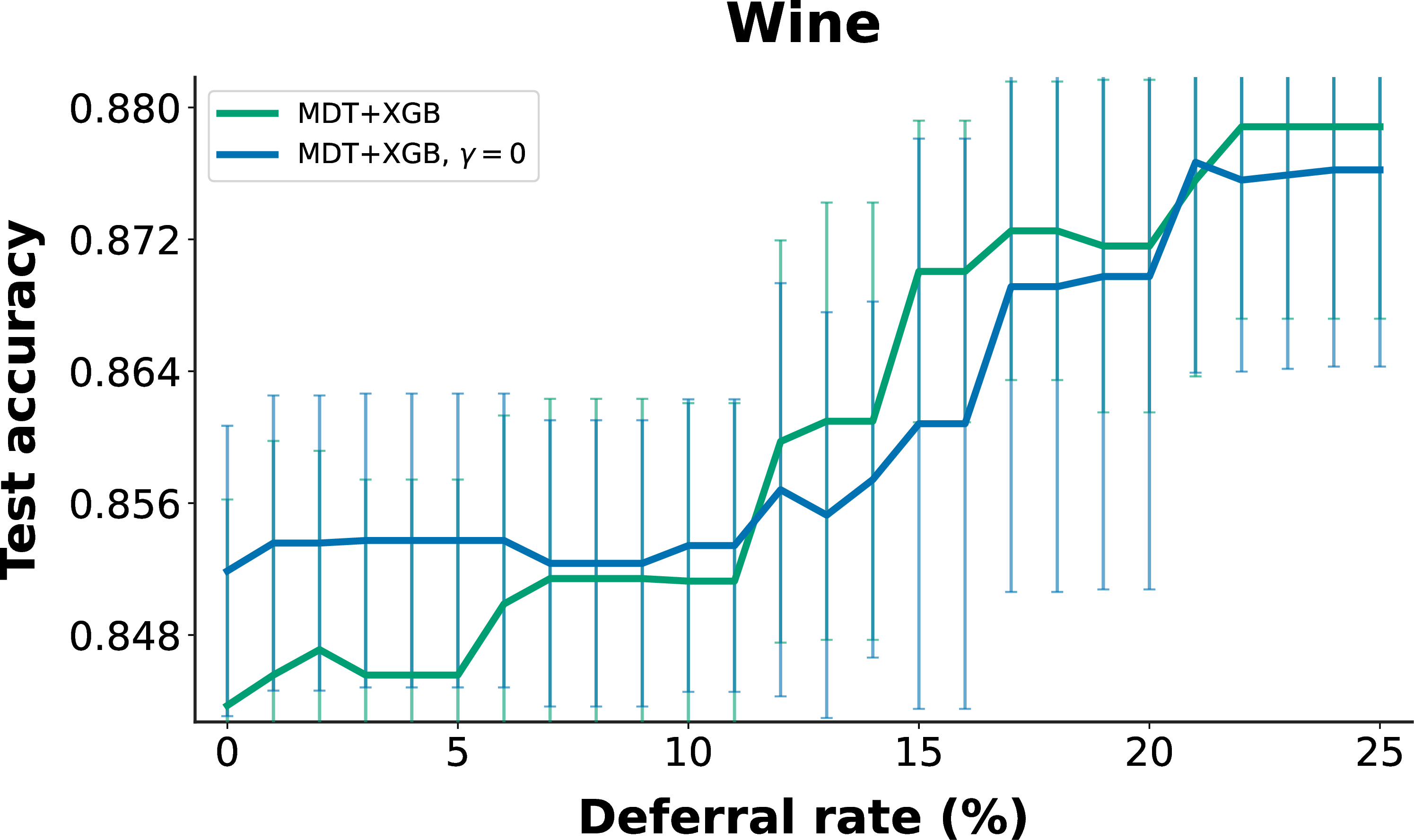
Figure 36: Ablation on the distance-based reweighting via tuning \(\gamma\) or setting \(\gamma=0\)..
| Dataset | MDT+XGB | MDT+XGB LeaveOneOut |
|---|---|---|
| Abalone | \(0.6333 \pm 0.0155\) | \(0.6323 \pm 0.0128\) |
| Adult | \(0.8681 \pm 0.0039\) | \(0.8661 \pm 0.0026\) |
| Aging | \(0.8028 \pm 0.0077\) | \(0.8028 \pm 0.0077\) |
| Bank | \(0.9090 \pm 0.0013\) | \(0.9077 \pm 0.0021\) |
| Bike | \(0.9493 \pm 0.0054\) | \(0.9427 \pm 0.0029\) |
| California | \(0.9099 \pm 0.0049\) | \(0.8997 \pm 0.0075\) |
5pt
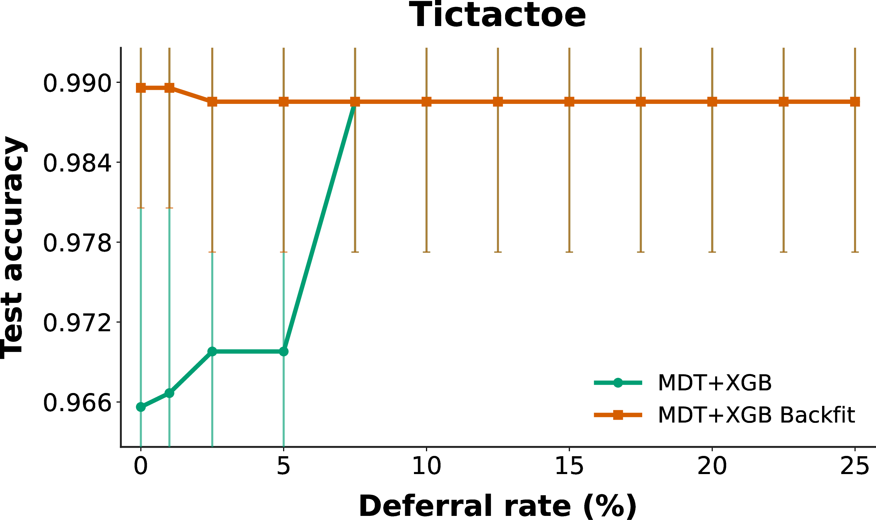

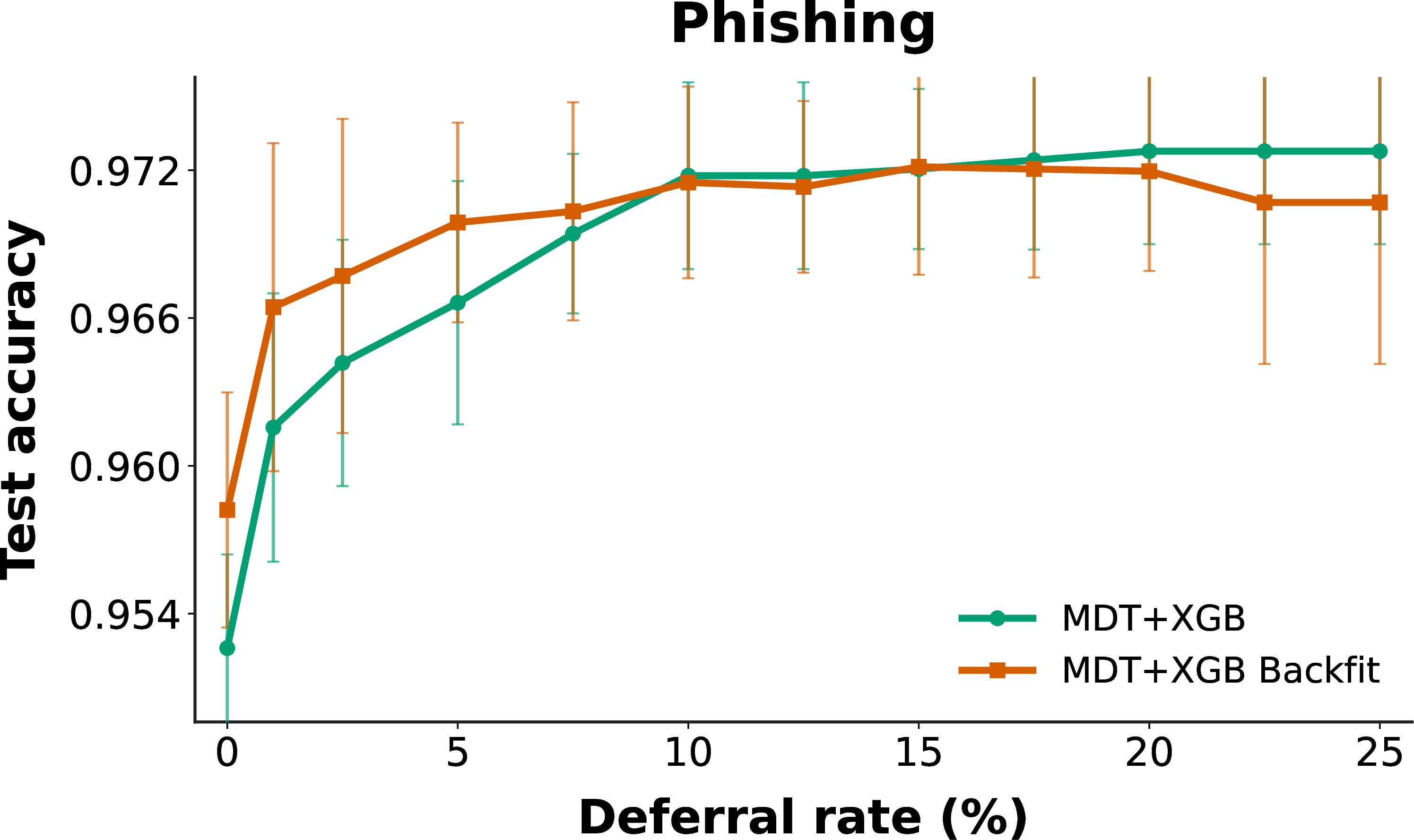
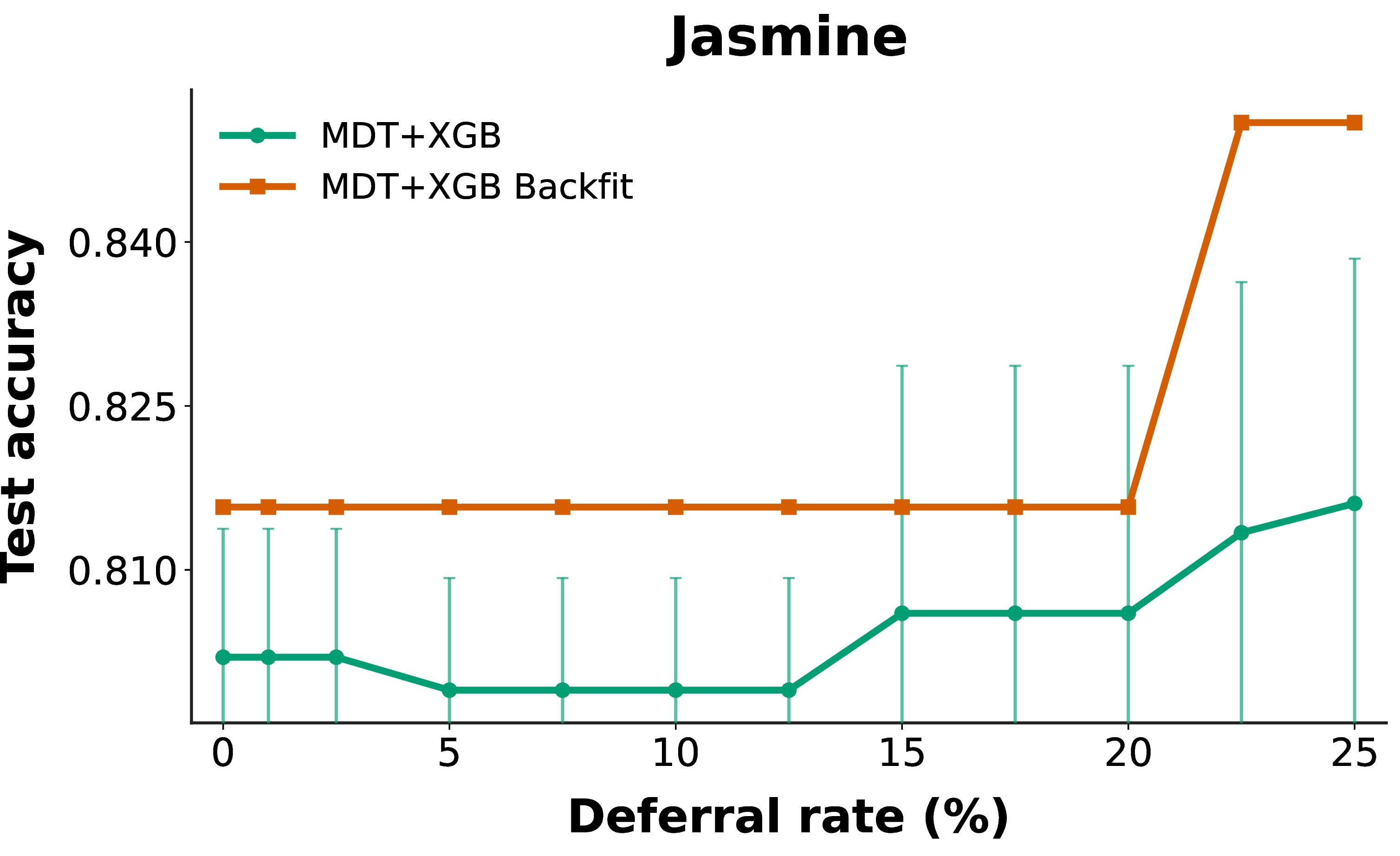
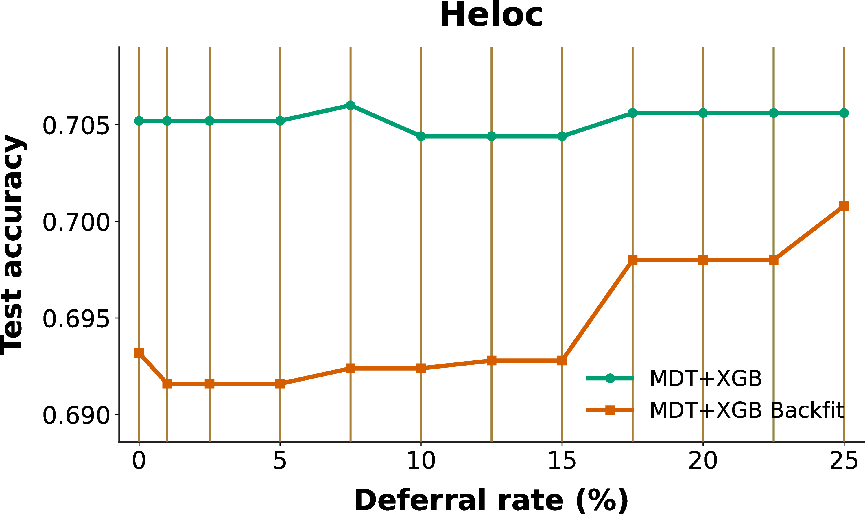

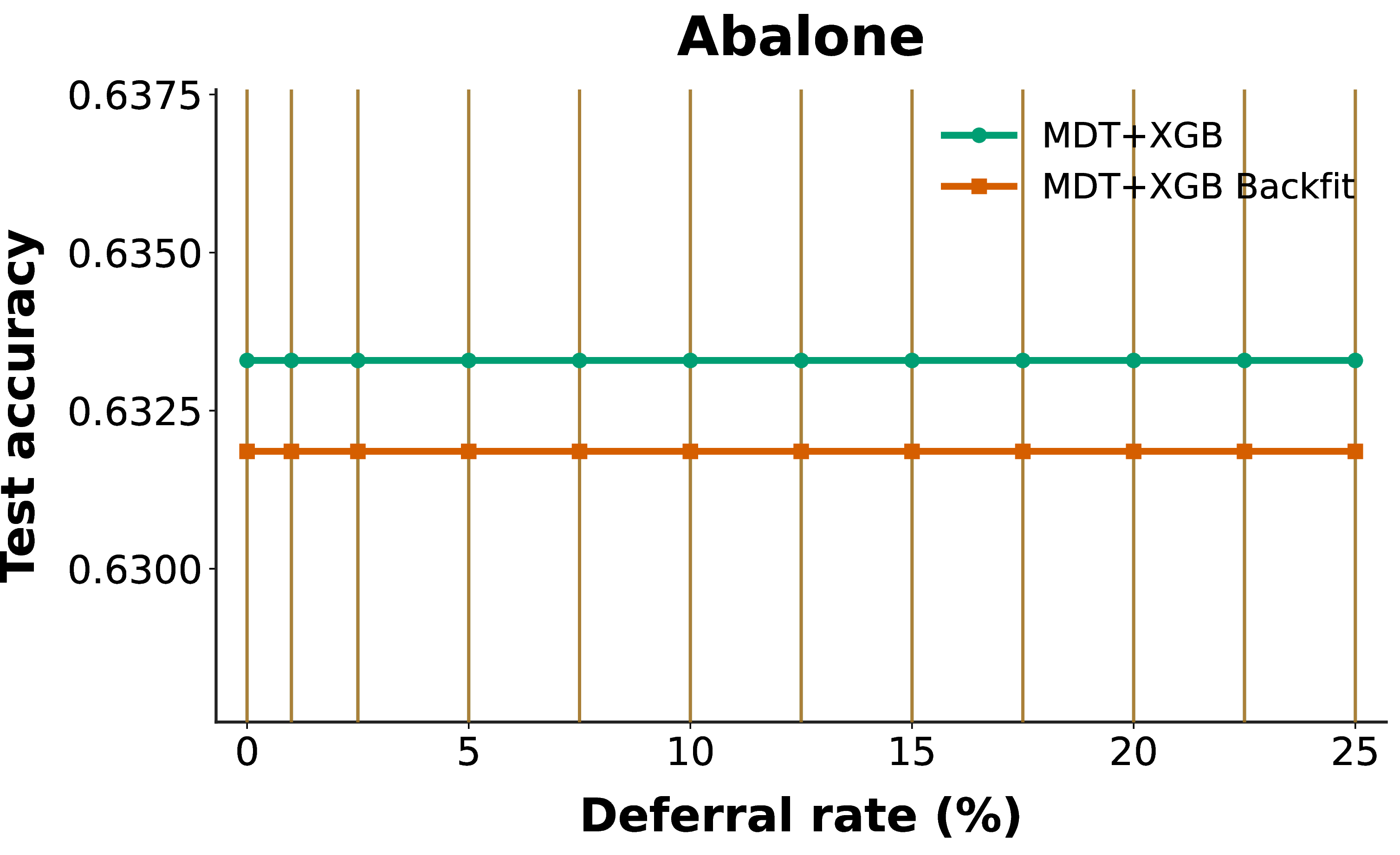
Figure 37: Comparison of MDT+XGB and MDT+XGB with backfitting across selected datasets. Each plot shows test accuracy as a function of the deferral rate. Backfitting gives clear improvements on some datasets, such as Tictactoe, where revisiting stages may help capture higher-order interactions, but it degrades performance on several others..
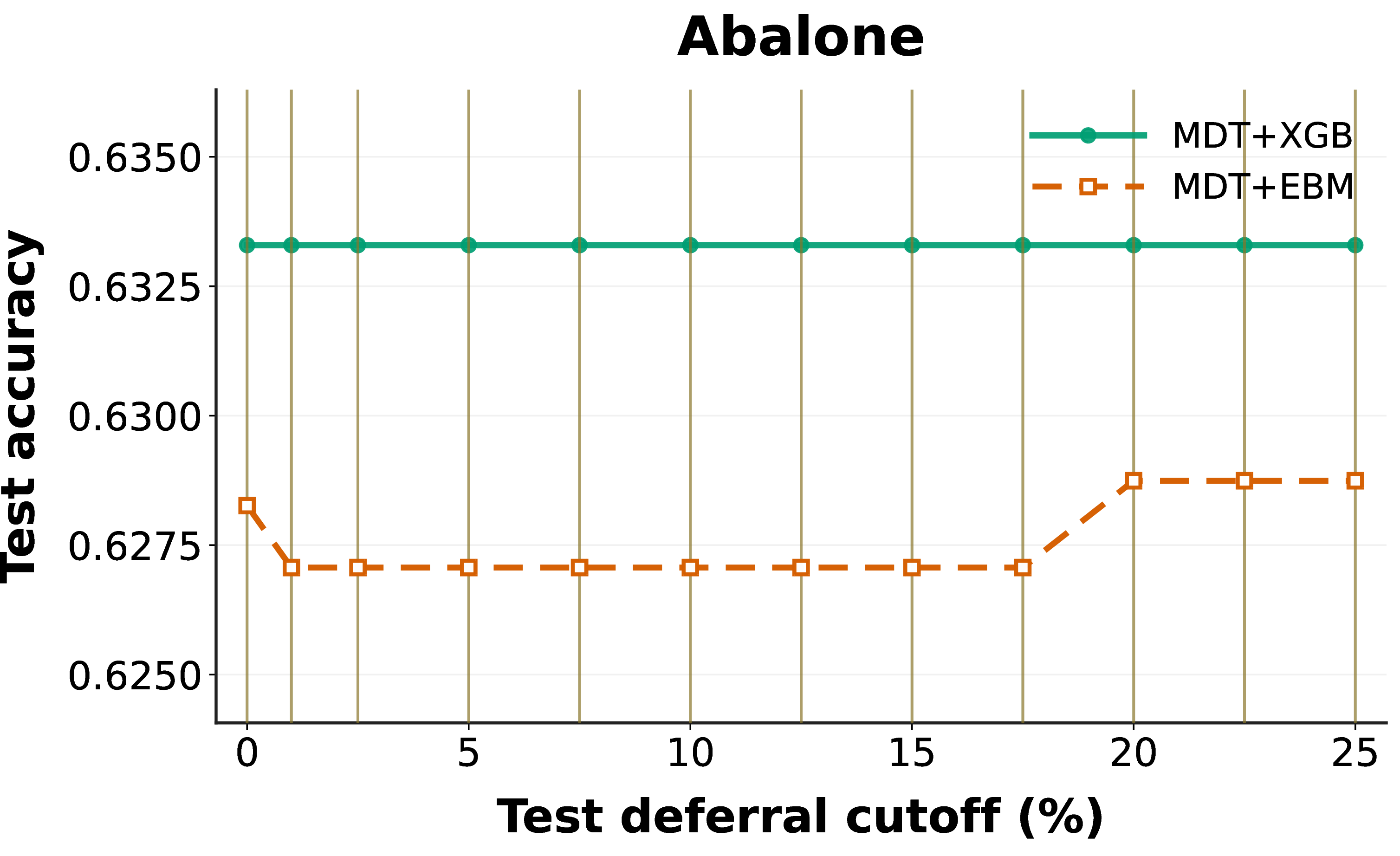
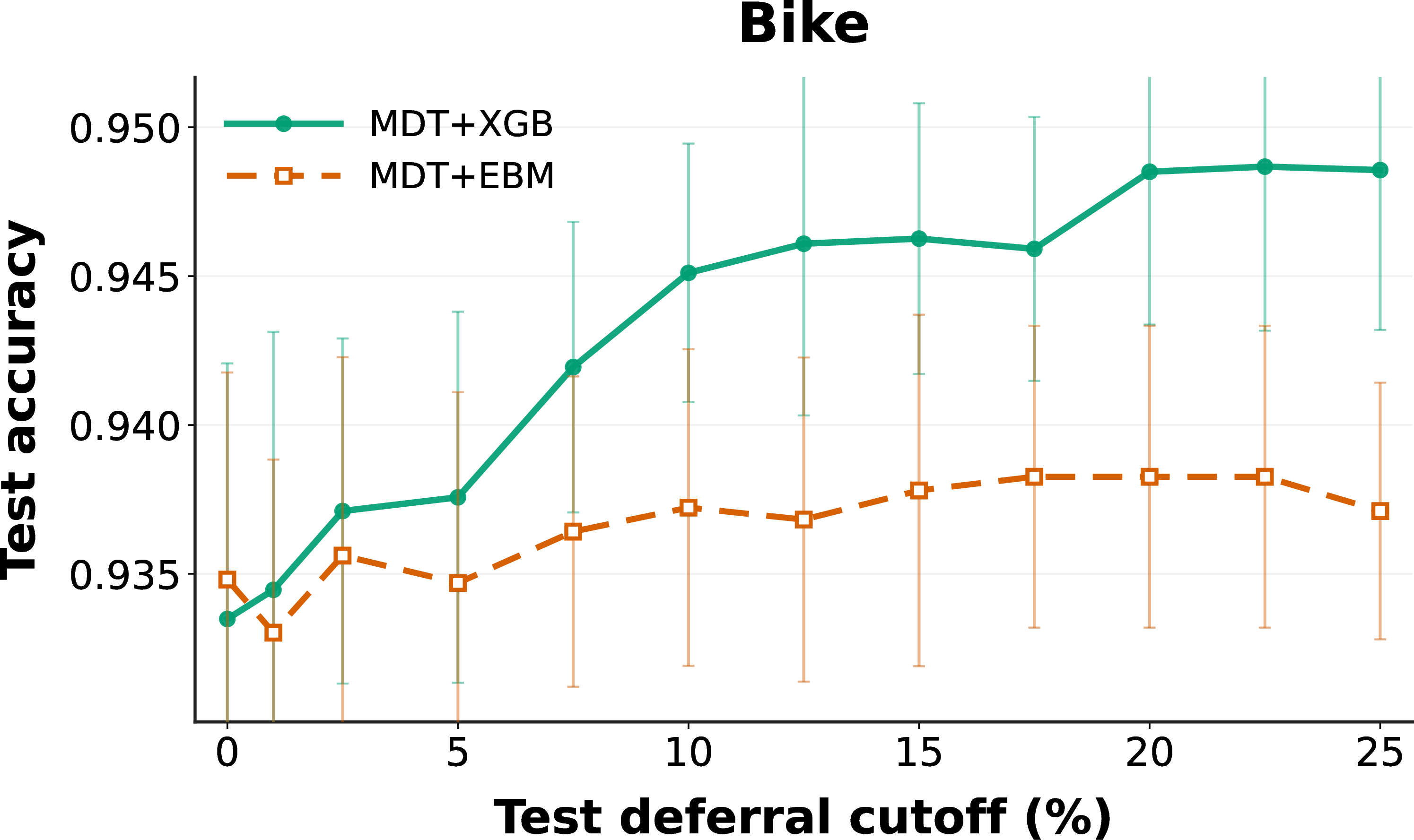


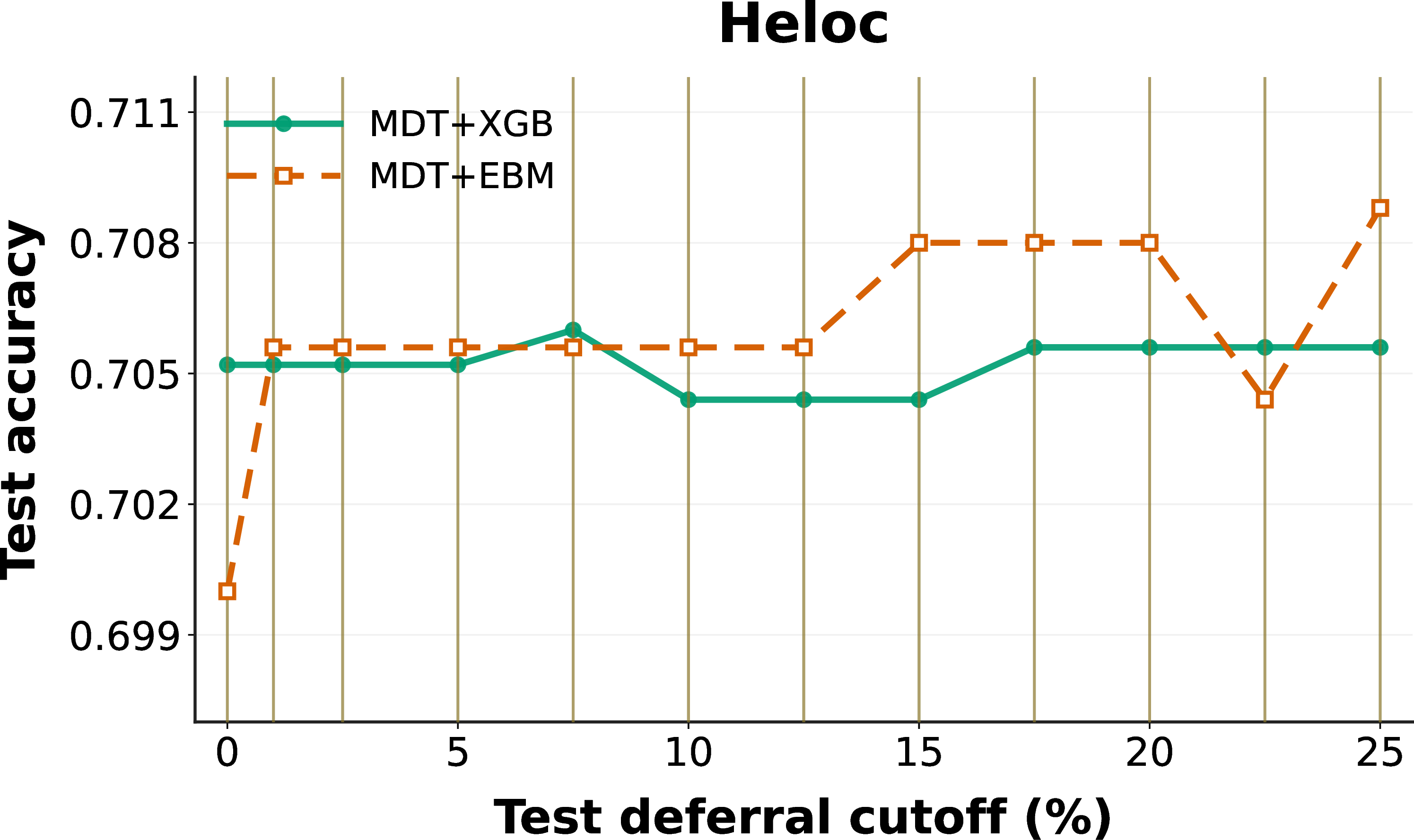
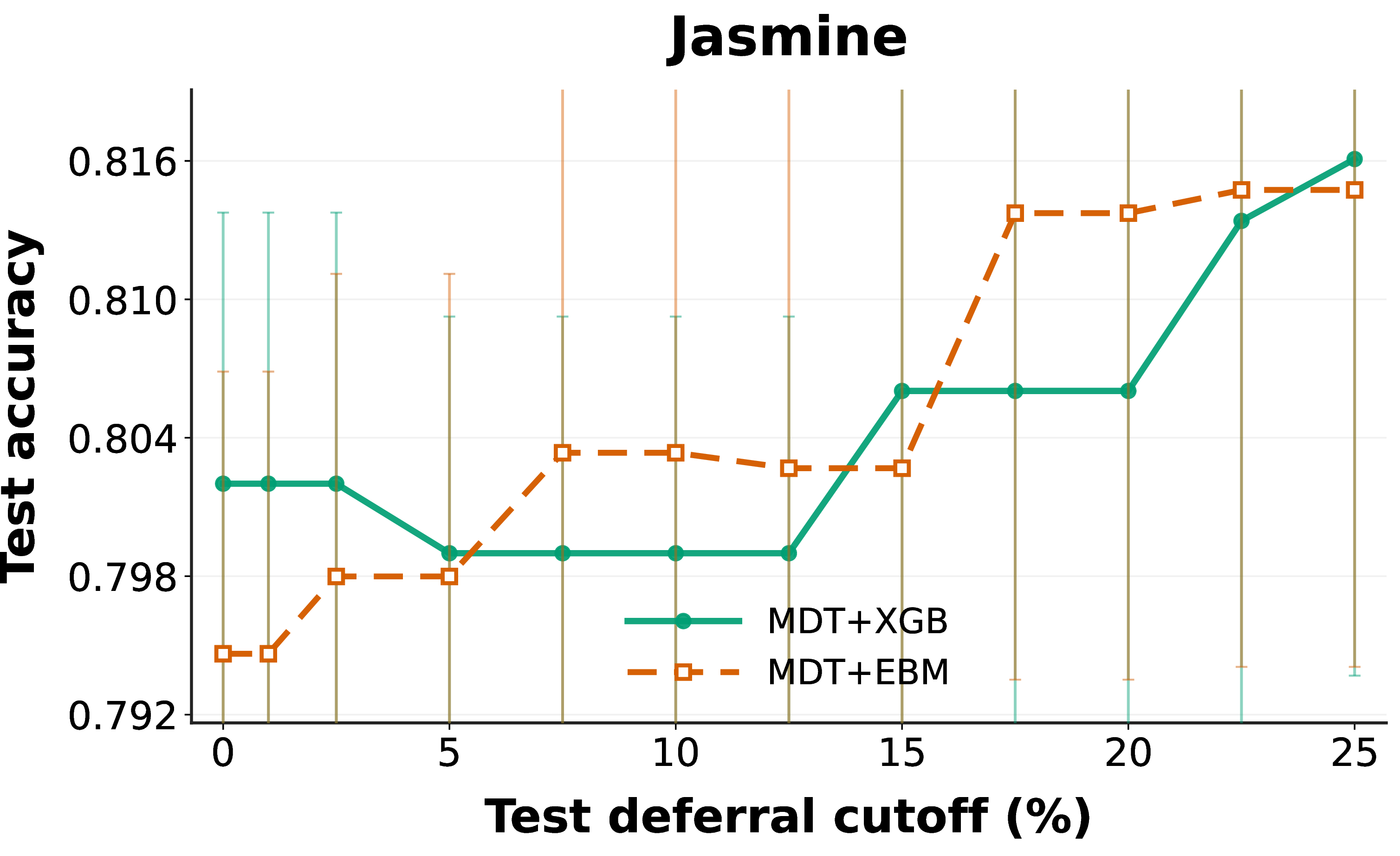
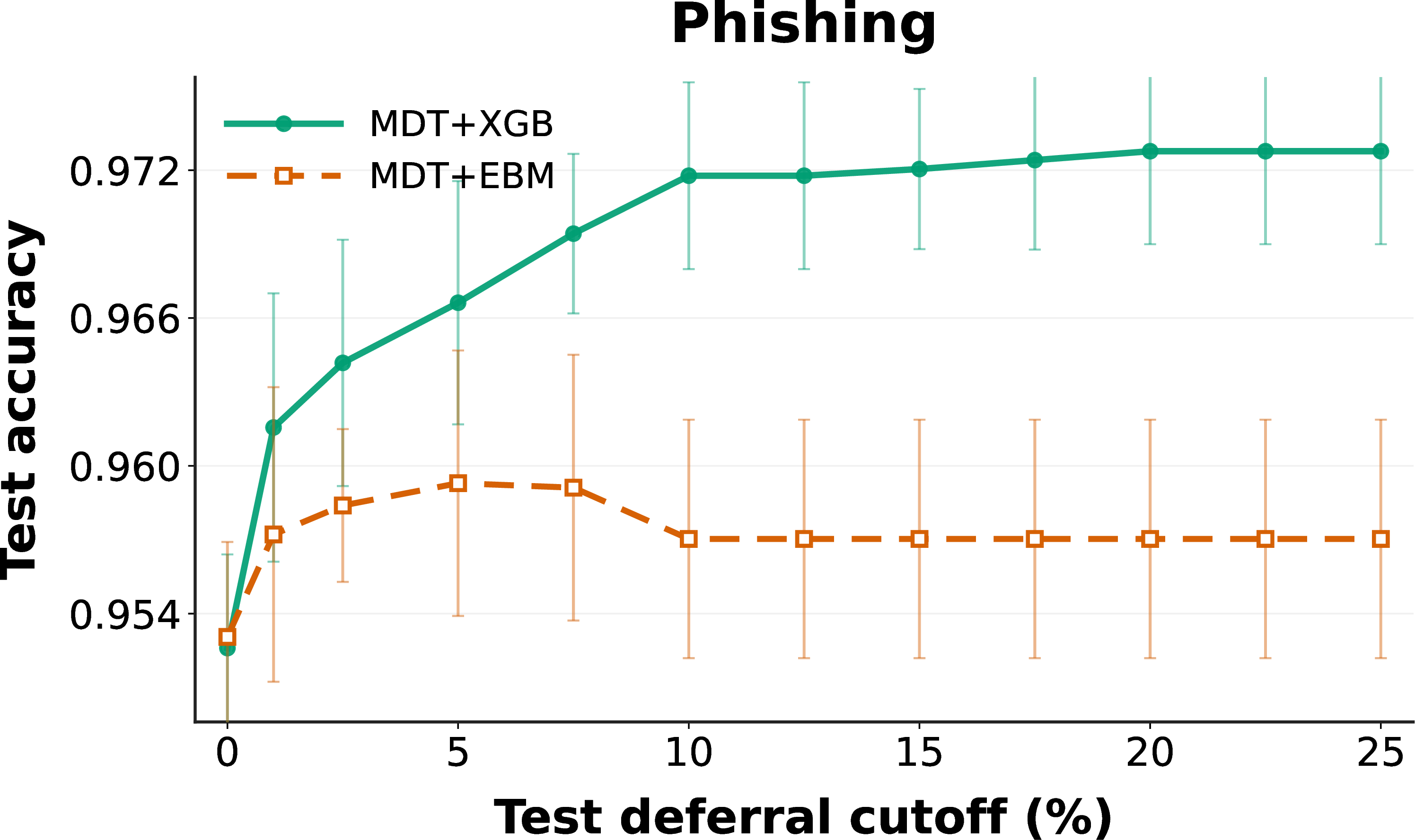
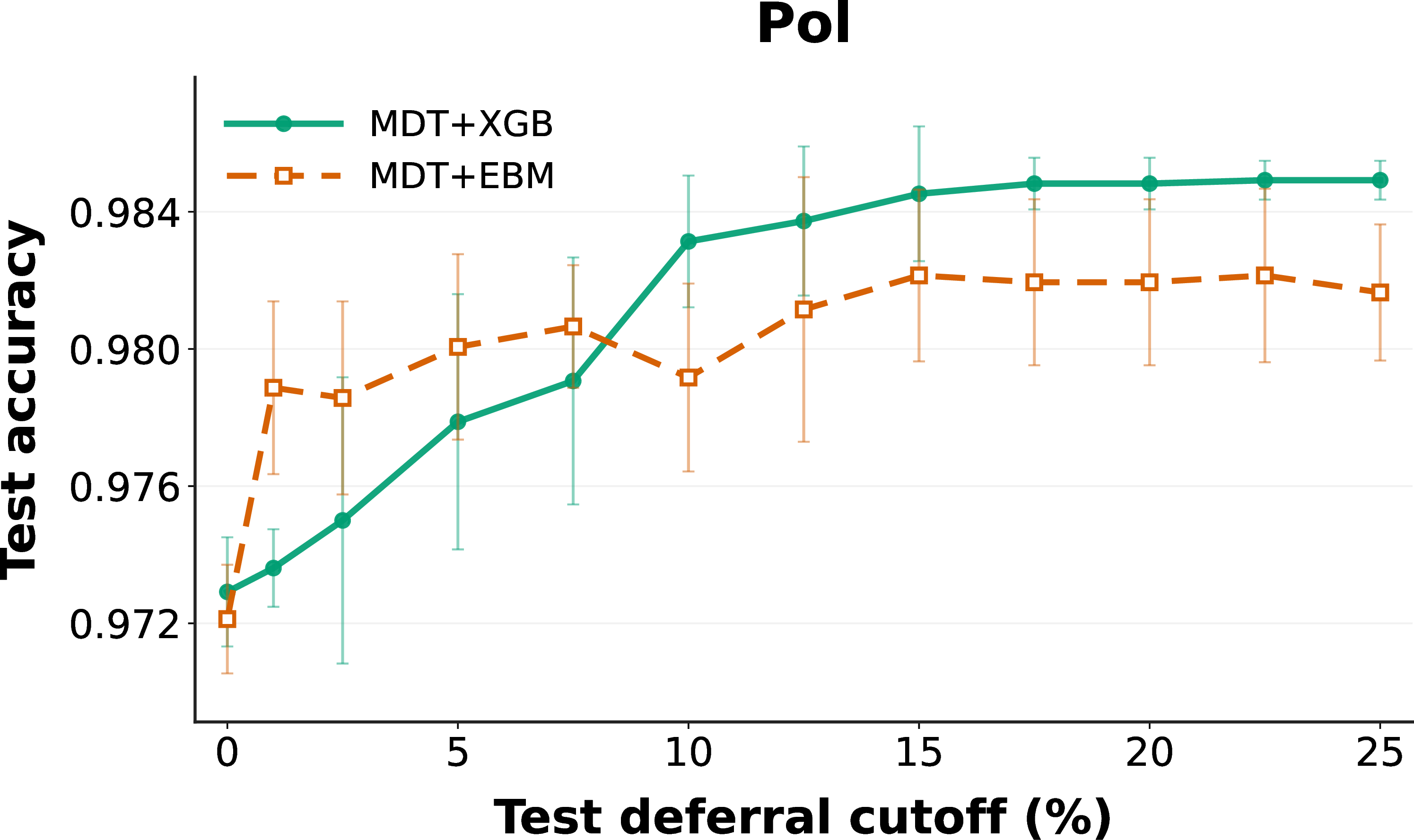
Figure 38: Comparison of MDT+XGB and MDT+EBM across selected datasets. MDT+EBM uses an Explainable Boosting Machine [10] as the fallback model, providing a more interpretable alternative to XGBoost. For some datasets, this amount of fallback complexity is sufficient, and MDT+EBM closely matches MDT+XGB. For other datasets, most notably Bike and Phishing, the EBM fallback is not expressive enough to recover the same accuracy–deferral tradeoff as MDT+XGB..
14 Examples of MDTs↩︎


Figure 39: Compressed MDT stages and corresponding compressed single-tree representation for Churn.. a — MDT stage 1, b — MDT stage 2, c — Compressed single-tree representation

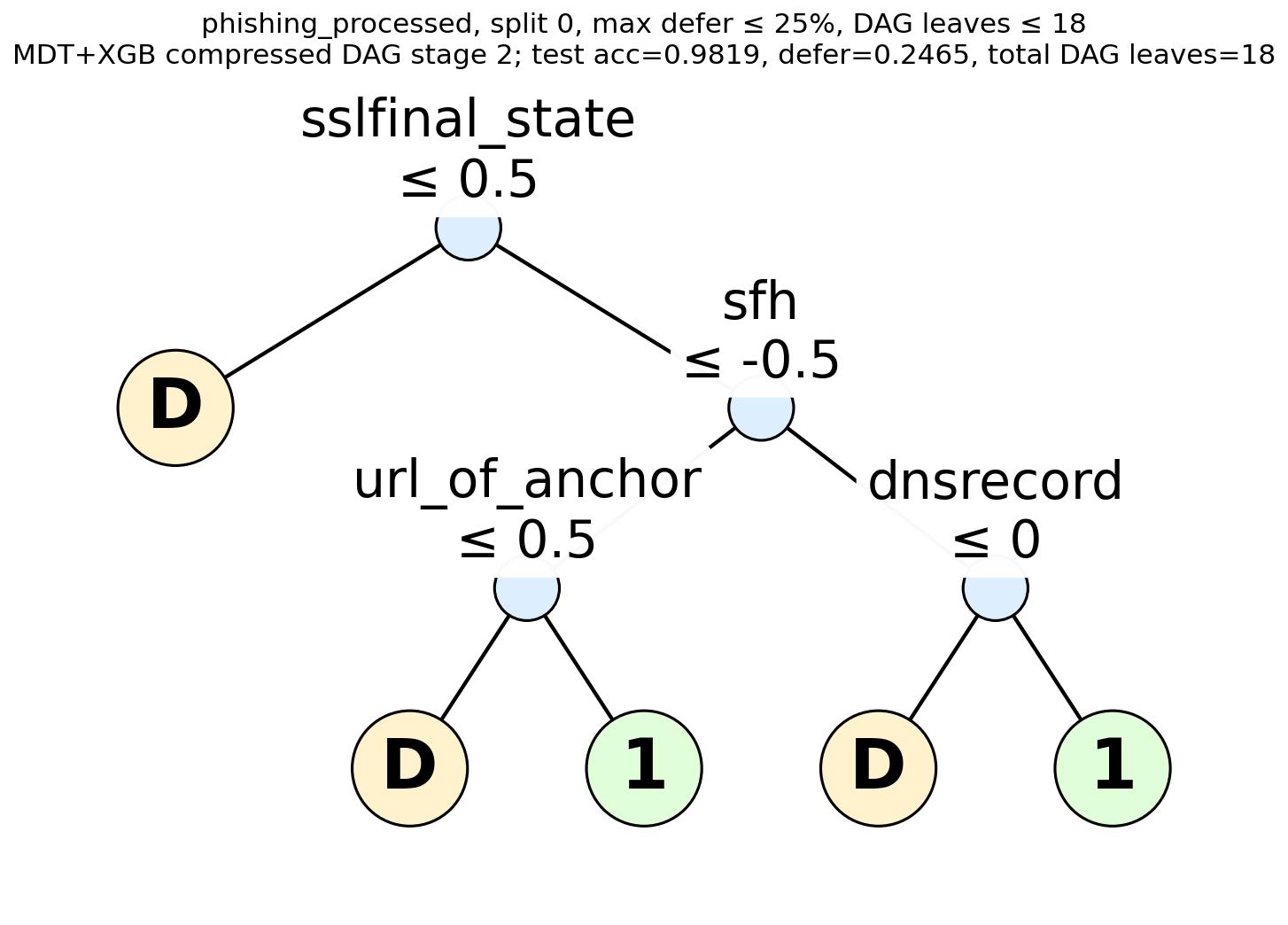
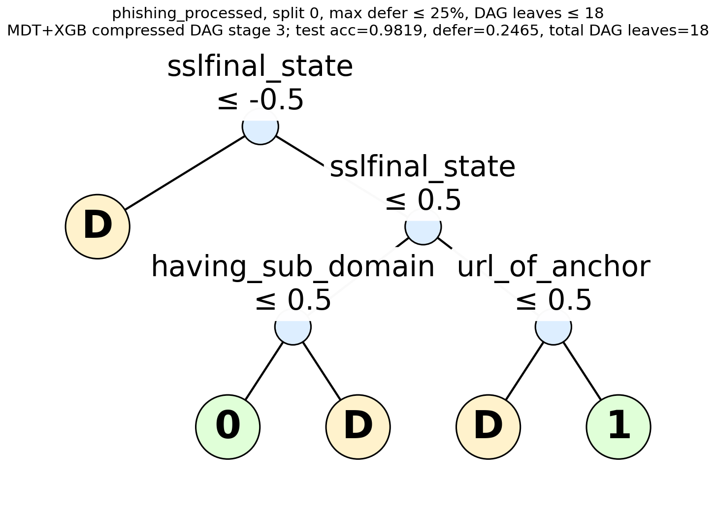
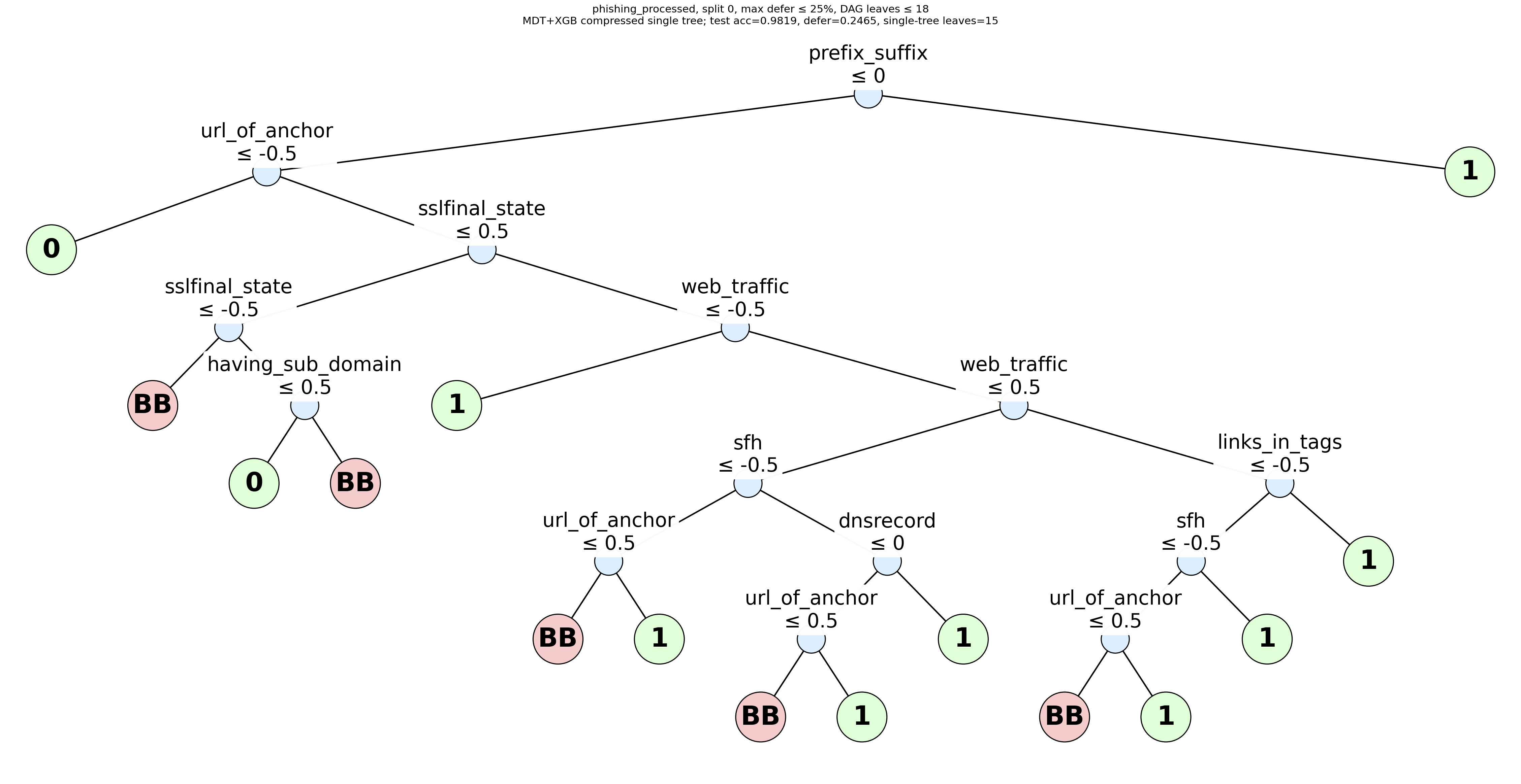
Figure 40: Compressed MDT stages and corresponding compressed single-tree representation for Phishing.. a — MDT stage 1, b — MDT stage 2, c — MDT stage 3, d — Compressed single-tree representation
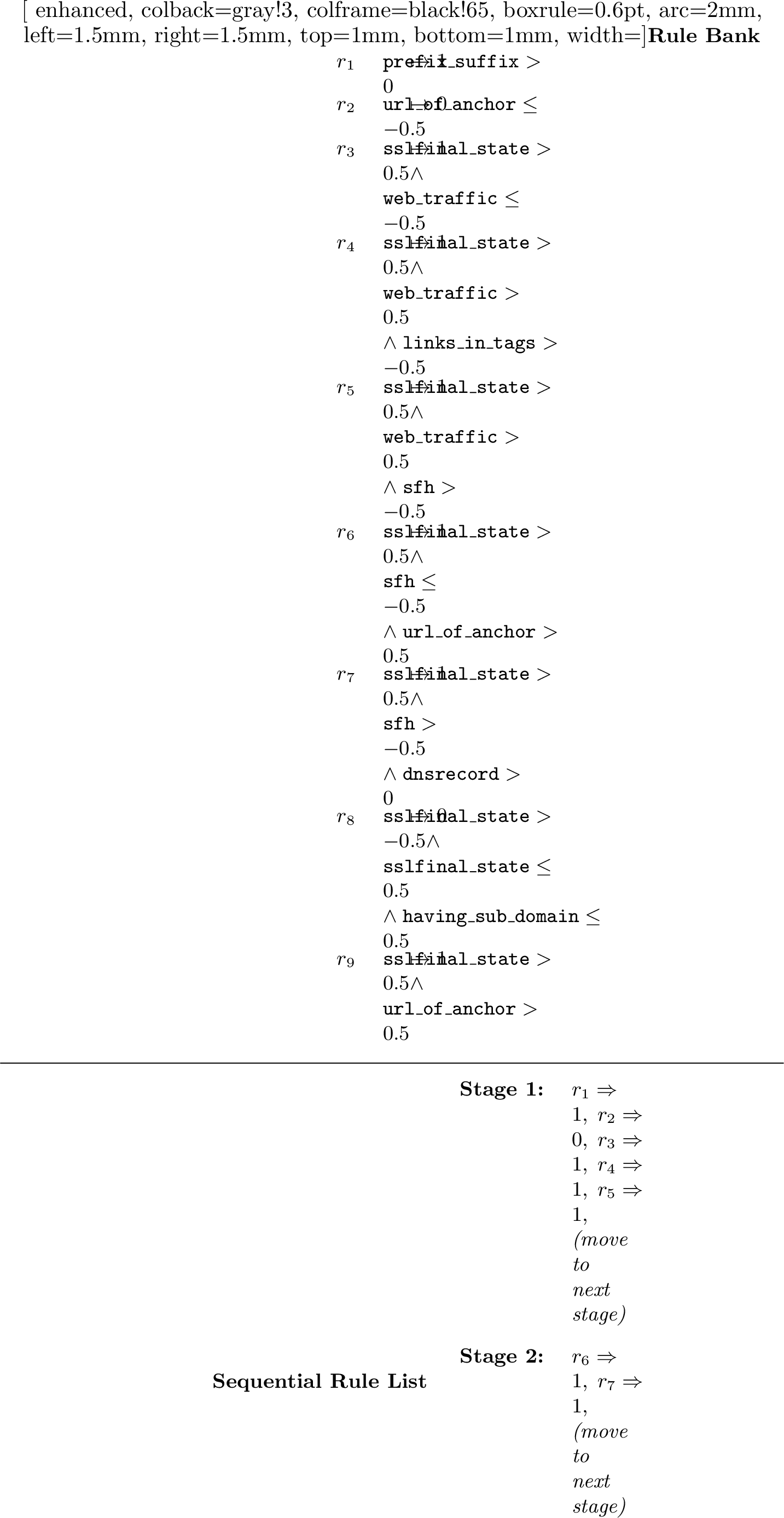
References↩︎
Equal contribution. Corresponding authors:
zakk.heile@duke.eduandhayden.mctavish@duke.edu.↩︎