RoPoLL: Robust Panel of LLM Judges
January 01, 1970
Abstract.
The LLM Jury, a Panel of LLM Evaluators (PoLL) [@verga2024replacing] reporting consensus scores, has become a practical alternative to single judge LLM
evaluation, yet its statistical behaviour remains poorly understood. We formalize the LLM Jury setup under the Huber contamination model, and show that PoLL incurs unbounded bias under any positive contamination, regardless
of jury size, whenever a single judge fails in a biased, LLM-typical way (mode collapse, sycophancy, safety refusal). We frame the jury consensus problem as an instance of classical robust mean estimation and propose RoPoLL
(Robust Panel of LLM-as-Judge), which preserves the PoLL panel and substitutes the aggregation function with a robust mean estimator. Among classical robust
estimators, we instantiate RoPoLL with the geometric median (GM), a tuning-free, joint-distance-preserving mean estimator that yields the optimal finite-sample breakdown point \(1/2\). We
establish a finite-sample error bound and an information-theoretic minimax lower bound that match on the parametric rate \(\sigma\sqrt{d/N}\) and differ on the breakdown floor by a factor of \(\sqrt{d}\) – a statistical-computational gap that polynomial-time RoPoLL pays relative to the (intractable) Tukey halfspace median. Across \(13\) open-weight
judges (\(4\) B–\(675\) B), three reward-model benchmarks, and four corruption regimes at rates up to \(50\%\), RoPoLL
dominates PoLL on every biased corruption type: by \(\approx 19\%\) on cross-dimensional attacks at matched compute, and by orders of magnitude on heavy-tailed Byzantine adversaries (whose
unbounded first moments make any breakdown-positive aggregator beat averaging unconditionally). A \(3\)-judge RoPoLL committee at \(38\) B beats
Mistral-Large-3 (\(675\) B) by \(1.31\times\) on HelpSteer-2 under \(30\%\) bimodal-random corruption – an \(18\times\) parameter advantage with strictly better accuracy. A Noisy-GT control confirms the premium is paid against biased contamination, not benign Gaussian imprecision (where PoLL is
statistically optimal). Overall, we establish that robust aggregation of a small, diverse committee is a parameter-efficient and statistically principled alternative to scaling a single large LLM-as-judge.
Correspondence:
1 Introduction↩︎
Reliable evaluation remains the bottleneck in aligning Large Language Models (LLMs). Human evaluation, while the gold standard, does not scale to the iterative development cycles that modern alignment pipelines demand. The field has therefore converged on the LLM-as-a-Judge paradigm [@zheng2023judging], in which another LLM (typically a frontier model) acts as a referee, scoring outputs along one or more quality attributes. Subsequent work has trained open judges to match this behaviour [@kim2024prometheus] and standardised rubric-based evaluation protocols [@li2023alpacaeval; @dubois2024alpacafarm; @ye2024flask]. A single judge, however, is a single point of statistical failure. The systematic biases its backbone exhibits, e.g., position, verbosity, self-enhancement, sycophancy, and refusal artefacts, are by now well documented [@wang2023large; @panickssery2024llm; @saito2023verbosity; @stureborg2024large]; they propagate uncorrected to every score, and the cost-quality profile of the resulting evaluation is fixed to that of the single model.
A natural remedy is to evaluate by committee. The LLM Jury, instantiated by the Panel of LLM Evaluators (PoLL) of [@verga2024replacing], ensembles smaller, diverse, cheaper backbones and reports the arithmetic mean of their scores as the consensus—sufficient, in their experiments, to match or exceed a single large judge. Related multi-model evaluators include peer-rank discussion [@li2024prd], multi-agent debate [@chan2024chateval], and deeper/wider judge networks [@zhang2024wider]; these vary the panel structure but inherit PoLL’s aggregation rule. PoLL is the optimal aggregator precisely when judge errors are light-tailed and centered on the truth, in which case averaging \(N\) judges contracts the variance at the parametric rate \(1/N\) (Proposition 1, §3.5); 11 (§6.5) shows the clean-baseline parameter-efficiency this delivers empirically.
1.0.0.1 The problem: Byzantine failures, not Gaussian noise.
Real LLM judges fail in ways that are nothing like Gaussian noise. A judge that produces malformed JSON triggers a parser fallback to the all-zeros score, dropping a single observation onto the boundary of the score space. A judge with sycophancy bias rates every response near the maximum, flattening genuine quality differences. A judge that handles one attribute well may catastrophically mis-score another, producing a vector that is plausible per axis yet jointly anomalous. A judge whose parser hallucinates can emit values entirely outside the bounded score scale. These four failure modes—mode collapse, sycophancy, cross-attribute confusion, and heavy-tailed hallucination—are all biased point masses far from the truth, not symmetric perturbations of it, and each occurs in real deployments at non-trivial rates: in our corpus, parser-failure alone reaches \(33\%\) on the smallest judge (Gemma-4B) for HelpSteer 3 multilingual prompts, with mean rates of \(3.4\%\) on HelpSteer 3 and \(0.6\%\) on HelpSteer 2 across the \(13\)-judge panel (2, §3.4).
This is the regime the classical robust-statistics literature [@huber1964robust; @tukey1960survey;
@small1990survey; @vardi2000multivariate; @minsker2015geometric; @lugosi2019sub] and Byzantine-robust optimisation literature [@blanchard2017machine; @yin2018byzantine; @elmhamdi2018hidden; @acharya2022robust; @acharya2025geometric] identify as the wrong regime for
PoLL-style aggregation. The Huber \({\epsilon}\)-contamination model (Assumption 2) admits all four failure modes
as specific instantiations of the contamination distribution \(Q_{i}\) (zeros, inverted, bimodal-random, and cauchy-far; mapped explicitly in §3.4 and evaluated in §6.2–6.4), and a direct calculation (Proposition 2, §3.6) shows that under any positive contamination rate PoLL’s conditional bias grows linearly with the corruption shift and is
unbounded over the corruption class, regardless of \(N\): the \(1/N\) variance reduction that motivates juries cannot rescue an aggregator whose bias is itself unbounded.
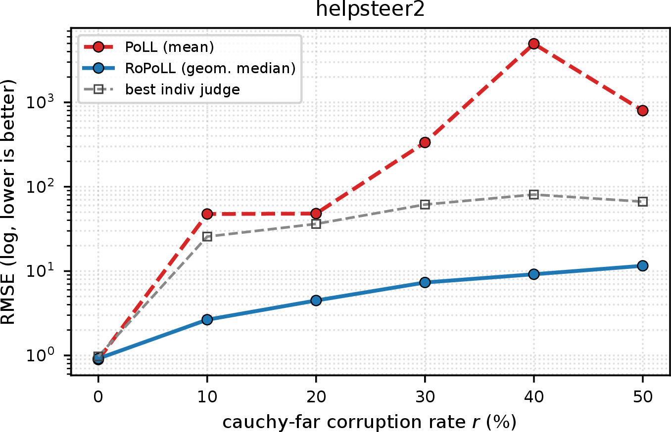
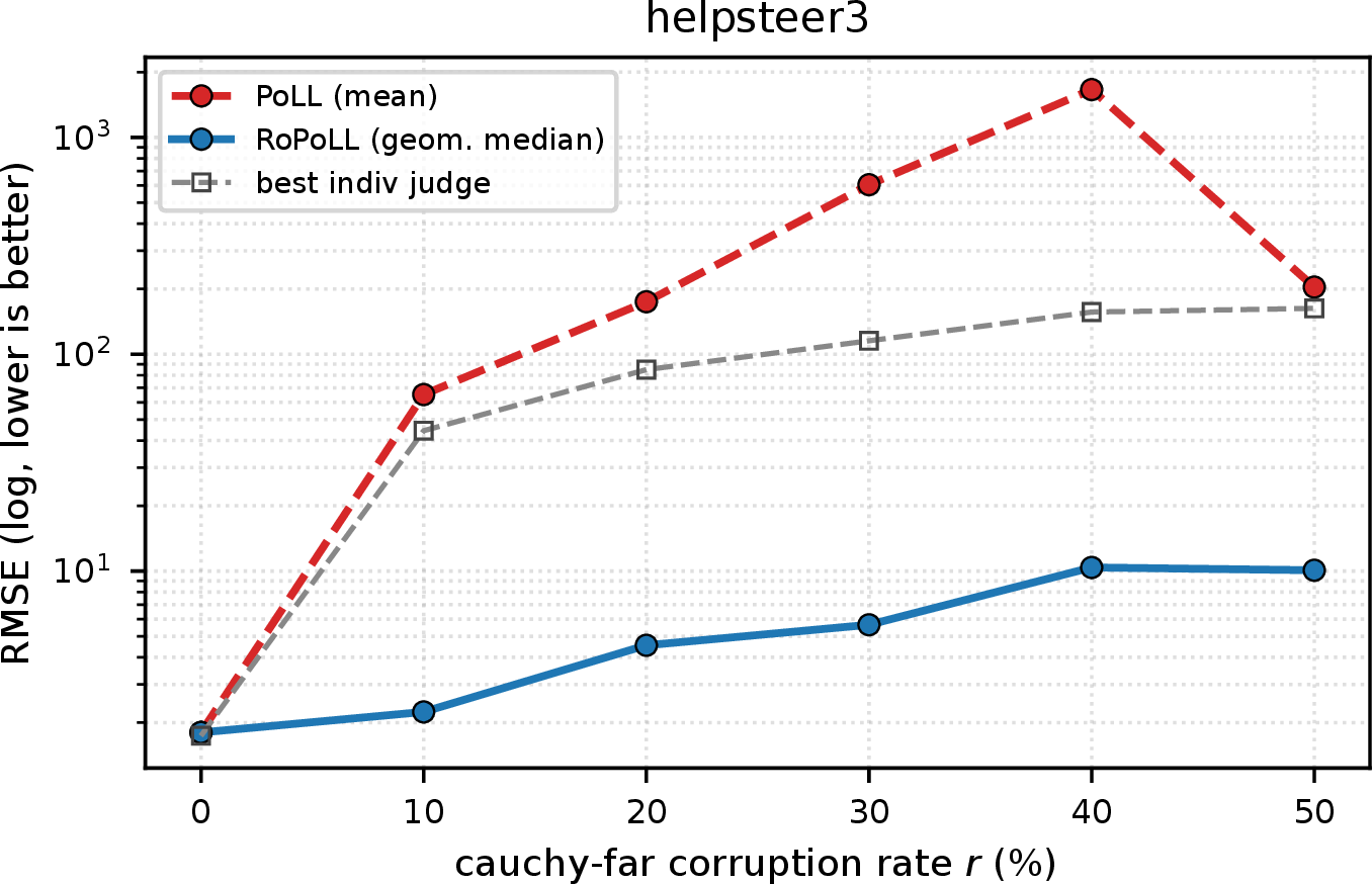
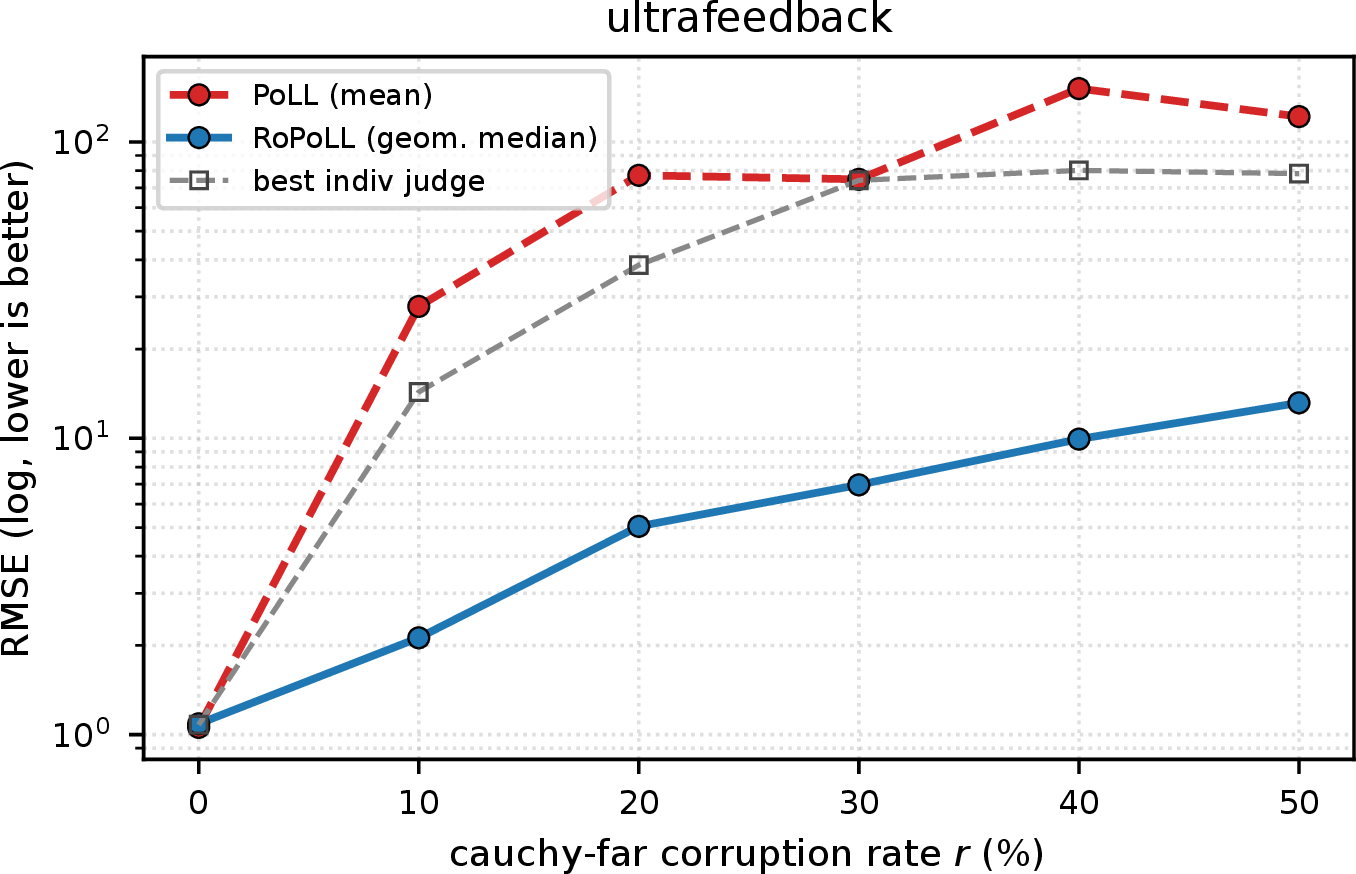
Figure 1: PoLL vs.RoPoLL under heavy-tailed cauchy-far corruption. RMSE vs.per-case corruption rate \(r\) (log \(y\)-axis) for the Medium jury (\(N{=}3\), \({\approx}89\) B), with the best single open-weight judge as a gray dashed reference;
coordinate-wise Median is competitive with RoPoLL here and is omitted (full three-method comparison in 13). Each corrupted slot is drawn as \(\hat{y} = y^{\star} + 10 + 2(s_{\max}{-}s_{\min})\,T\) with \(T\) component-wise standard Cauchy: a biased heavy-tailed Byzantine attack with undefined mean and variance, instantiating the
adversarial choice in Proposition 2.. a — HelpSteer 2, b — HelpSteer 3, c — UltraFeedback
1.0.0.2 Overview of our approach.
We propose RoPoLL (Robust Panel of LLM-as-Judge), a drop-in replacement for the arithmetic-mean aggregation step of PoLL with a robust mean estimator. Among classical candidates—the coordinate-wise median (CoMed), the trimmed mean, and the geometric median (GM)—only GM is simultaneously tuning-free (no contamination-rate hyperparameter unlike the trimmed mean), joint-distance preserving (operates on Euclidean distance over the full score vector unlike CoMed, which decouples coordinates and misses cross-attribute structure of Example 1), and attains the optimal \(1/2\) breakdown point (Definition 8, Proposition 3); the comparison is developed in detail in §4.1. We instantiate RoPoLL with the geometric median (Definition 7), computed via the modified Weiszfeld iteration (Algorithm 4, §4.3) at \(O(Nd\log(1/{\epsilon}))\) per query. CoMed and the trimmed mean serve as empirical baselines in §6.
1.0.0.3 Contributions.
Formalisation. We give the first formal treatment of LLM jury aggregation as a robust mean-estimation problem (§3): we model the LLM-as-Judge pipeline as a Markov kernel (Definition 4), define the LLM Jury (Definition 5), and characterise judge failures as Byzantine faults under the Huber contamination model (Assumption 2). Proposition 2 shows that PoLL admits unbounded bias under this model.
Algorithm and theory. We propose RoPoLL (§4) and establish its theoretical guarantees (§5): a finite-sample upper bound \(\|\hat{{\mathbf{y}}}_{\mathrm{GM}}-{\mathbf{y}}^{\star}\|_{2} \leq C_{\alpha+\beta}\rho\) with explicit absolute constants (Theorem 1), a correlated-jury extension under the equicorrelated-indicator hypothesis (Lemma 3, with empirical indicator-correlation \(\bar\gamma_{W} \in [0.45, 0.53]\) measured on our judge panels, 6.10), and an information-theoretic minimax lower bound (Theorem 2) that matches on the parametric rate \(\sigma\sqrt{d/N}\) and differs on the breakdown floor by a \(\sqrt{d}\) statistical–computational gap, attributed to GM’s polynomial-time tractability relative to the (intractable) Tukey halfspace median.
Large-scale empirical validation. We evaluate \(13\) open-weight LLM judges spanning four model-size tiers (\(4\) B–\(675\) B parameters) on three benchmarks with complementary ground-truth sources: HelpSteer 2 [@wang2024helpsteer2], HelpSteer 3 [@wang-etal-2025-helpsteer3], and UltraFeedback [@cui2024ultrafeedback]. Under systematic adversarial injection at contamination rates up to \(50\%\) (§6), RoPoLL outperforms PoLL by up to three orders of magnitude on biased heavy-tailed (
cauchy-far, 1) and cross-dimensional (bimodal-random, 9) attacks; a \(3\)-judge RoPoLL committee at \(38\) B total parameters beats Mistral-Large-3 (\(675\) B) by \(1.31\times\) on HelpSteer 2 under \(30\%\)bimodal-randomcorruption (an \(18\times\) parameter advantage, §6.3). A Noisy-GT control (§6.7) rules out the obvious confound that the RoPoLL premium is paid against benign Gaussian imprecision rather than against biased contamination.Open release of the judge-output corpus. 2 We release the full \(13\)-judge \(\times\) three-benchmark output corpus—approximately \(28\mathrm{K}\) scored \((\text{judge}, \text{sample})\) cells of parsed attribute scores, per-call latencies, and reference labels underlying every figure in §6 (§6.8). To our knowledge this is the first standardised corpus of LLM-jury outputs; follow-up work on judge calibration, alternative aggregators, or new corruption families can be benchmarked against this fixed substrate without re-running the inference cost.
1.0.0.4 Paper organisation.
§3 formalises the problem setup, including the LLM Jury (Definitions 4–5), the Huber contamination model (Assumption 2, with the empirical natural-failure-rate calibration of 2), and the unbounded-bias result for PoLL (Proposition 2). §4 develops the RoPoLL methodology: the choice of geometric median over coordinate-wise median and trimmed mean (§4.1), structural properties of GM (Proposition 3), and the Weiszfeld iteration (Algorithm 4). §5 states the finite-sample upper bound (Theorem 1), its correlated-jury extension (Lemma 3), and the matching minimax lower bound (Theorem 2). §6 presents the benchmark evaluation organised by corruption type; §2 situates the work in the LLM-as-Judge, robust-statistics, and Byzantine-distributed-learning literatures; §7 concludes with scope, limitations, and follow-up directions. The released corpus and its inter-judge correlation structure, including the empirical \(\bar\gamma_{W}\) measurement, are documented in §6. Full proofs and a 2D synthetic visualisation gallery are deferred to Appendices 8–9.1.
2 Related Work↩︎
LLM-as-Judge evaluation and per-judge biases. The LLM-as-Judge paradigm was established by [@zheng2023judging] (MT-Bench, Chatbot Arena), demonstrating that strong models such as GPT-4 can serve as reliable proxies for human annotators. Subsequent work has extended the paradigm along several axes: open-source judges with fine-grained rubrics [@kim2024prometheus]; automated frameworks for instruction-following models [@li2023alpacaeval; @dubois2024alpacafarm]; and skill-level evaluation [@ye2024flask]. A parallel literature documents systematic biases of single judges—position, verbosity, self-enhancement, sycophancy, and prompt-format sensitivity [@wang2023large; @panickssery2024llm; @saito2023verbosity; @stureborg2024large]. These findings motivate the use of diverse judge panels but treat each judge in isolation; no prior work analyzes the aggregation step or its failure modes.
Jury and panel evaluation. [@verga2024replacing] introduced the Panel of LLM Evaluators (PoLL), our direct predecessor: a diverse committee of smaller backbones aggregated by the arithmetic mean. Their work established the practical value of LLM juries but did not analyze robustness; the mean aggregator is used without justification, and no failure modes are considered. [@zhang2024wider] studied how panel width and depth affect evaluation fairness, again without robustness guarantees. The key gap across this literature is the absence of any analysis of catastrophic failure modes or formal robustness properties of the aggregation rule. Our Proposition 2 closes this gap: under any positive contamination rate PoLL [@verga2024replacing] admits unbounded bias regardless of \(N\).
Multi-agent debate and structured aggregation. A distinct family of multi-judge methods produces aggregated judgments through structured interaction rather than independent scoring. [@li2024prd] propose peer-rank discussion among judges, in which each judge sees others’ scores and updates its own; [@chan2024chateval] propose multi-agent debate, in which judges argue over a verdict before consensus. These methods change the joint distribution of \((\hat{{\mathbf{y}}}_{1}, \ldots, \hat{{\mathbf{y}}}_{N})\)—they introduce dependence by design, breaking Assumption 3—and trade independence for deliberation-driven error reduction. Whether they exhibit the same Byzantine-failure mode as PoLL is an open question. The Huber-contamination analysis of this paper does not directly apply to such interactive aggregators, but the corruption-class diagnosis (point masses far from the truth) likely transfers, suggesting robust extensions of debate-based aggregation as a future direction. Majority voting in mathematical reasoning [@cobbe2021training] is a related but coarser ensemble technique on binary correctness; the analogue of Proposition 2 for vote-based aggregation on \(\{0, 1\}\) outputs is the standard \(\alpha < 1/2\) Byzantine threshold.
Calibration as a complementary paradigm. A separate line of work removes judge bias at the source via per-judge calibration on a labeled validation slice [@zheng2023judging]. Calibration assumes a stationary, recoverable bias and trades worst-case guarantees for average-case efficiency; RoPoLL assumes nothing on the corruption distribution and pays a constant-factor insurance premium to bound the worst case. The two are complementary: RoPoLL can aggregate calibrated scores, and the calibration-RoPoLL composition—together with extensions to heterogeneous, correlated, and dependent juries—is left to future work.
Robust statistics and the geometric median. The Huber contamination model [@huber1964robust] and the breakdown point [@tukey1960survey] are the classical framework for estimation under arbitrary corruption. The geometric median attains the optimal \(1/2\) breakdown for any translation-equivariant estimator [@lopuhaa1991breakdown; @small1990survey; @vardi2000multivariate]; in high dimensions, [@minsker2015geometric] established sub-Gaussian concentration for the geometric median of means—the result Theorem 1 adapts to contaminated juries—and [@lugosi2019sub] developed sub-Gaussian mean estimators with optimal dimension dependence. Recent applications to ML pipelines include block-coordinate GM descent for robust training [@acharya2022robust] and GM Matching for robust subset selection [@acharya2025geometric]; [@acharya2025robust] surveys robust learning from noisy data. Our setting differs from this literature on three axes: (i) low dimension (\(d \in \{4, 5\}\) evaluation attributes, so the \(\sqrt{d/N}\) rate is dominated by constants and the \(1/(1-2\alpha)\) contamination factor is the load-bearing dependence); (ii) structured contamination (\(Q_{i}\) arises from specific LLM failure modes—parser fallback, sycophancy, refusals, cross-attribute confusion—which inform the four empirical corruption types in §6); and (iii) heterogeneous workers (per-judge \(\sigma_{i}, \alpha_{i}\) vary across the panel, outside the i.i.d. regime that the classical robust-statistics literature targets). Among broader alternatives in the robust-aggregation toolbox, the half-space (Tukey) median attains the optimal breakdown \(1/2\) in any dimension but is NP-hard to compute and prohibitive at \(d \geq 5\) [@small1990survey]; median of means [@lugosi2019sub] targets heavy-tailed data rather than Huber contamination concentrated in a minority of judges; the geometric median’s tuning-free \(1/2\) breakdown, joint-distance objective, and \(O(Nd\log(1/{\epsilon}))\) cost make it the right default for the small-\(d\), small-\(N\), heterogeneous-worker, one-shot regime that LLM juries occupy. A systematic empirical comparison against the broader family is left to future work (§7).
Byzantine-robust distributed learning. The connection between robust aggregation and Byzantine fault tolerance has been worked out in distributed optimization: Krum [@blanchard2017machine], coordinate-wise median and trimmed mean as gradient aggregators [@yin2018byzantine], and Bulyan [@elmhamdi2018hidden]. This literature targets \(N\) from tens to thousands of workers, with adversarial perturbations composed across thousands of training rounds. The LLM-jury setting shares the mathematical structure but differs operationally on three axes: (a) small \(N\) (juries operate at \(N \in \{3,\dots,13\}\) where every judge is materially expensive, requiring tight finite-sample guarantees); (b) per-sample heterogeneity (the contamination indicator \(Z_{i}\) is conditional on the prompt-response pair \(x\), not per round); (c) no iterative learning loop (LLM-jury aggregation is one-shot at evaluation time, so the per-instance bias bound matters directly rather than its cumulative effect across rounds). These differences explain why our analysis emphasizes finite-sample distribution-free guarantees over the corruption class (Theorem 1); the heterogeneity of the worker pool, judge correlation, and explicit dependence (in debate-based methods) are left to future work and have no direct analogue in the Byzantine distributed-learning literature.
To our knowledge, we are the first to formalize LLM jury aggregation as a robust estimation problem, prove finite-sample contamination guarantees in this setting, and evaluate robustness systematically against both natural and adversarial judge failures at scale.
3 Problem Setup↩︎
We evaluate a system agent \({\mathcal{M}}: {\mathcal{P}}\to {\mathcal{R}}\) that maps prompts to responses. For each evaluation instance \(x = (p, r) \in {\mathcal{X}}\triangleq {\mathcal{P}}\times {\mathcal{R}}\) the goal is to estimate a vector of attribute scores describing how good the response \(r\) is for the prompt \(p\).
3.1 System Agent and Reward Space↩︎
Let \({\mathcal{P}}\) and \({\mathcal{R}}\) denote the spaces of admissible natural-language prompts and responses, and define the instance space \({\mathcal{X}}\triangleq {\mathcal{P}}\times {\mathcal{R}}\). The model under evaluation is the system agent \({\mathcal{M}}: {\mathcal{P}}\to {\mathcal{R}}\), \(p \mapsto {\mathcal{M}}(p)\). Given a prompt \(p\), the realized response is \(r = {\mathcal{M}}(p)\) and the evaluation instance is \((p, r) \in {\mathcal{X}}\). Any stochasticity in the underlying generation procedure is immaterial for the development below, which is carried out conditional on the realized pair \((p, r)\).
Definition 1 (Reward). Fix \(d \in \mathbb{N}\) and write \([d] \triangleq \{1, \ldots, d\}\). For each \(k \in [d]\), let \({\mathcal{Y}}^{(k)}\) be a measurable space encoding the admissible judgements for attribute \(k\). The reward space* is the Cartesian product \({\mathcal{Y}}\triangleq \prod_{k=1}^{d} {\mathcal{Y}}^{(k)}\), and a reward associated with \((p, r) \in {\mathcal{X}}\) is a vector \({\mathbf{y}}= (y^{(1)}, \ldots, y^{(d)}) \in {\mathcal{Y}}\) where \(y^{(k)} \in {\mathcal{Y}}^{(k)}\) records the judgement of \(r\) on attribute \(k\).*
Definition 1 does not impose a common structure across the coordinate spaces, and typical instantiations include bounded scalars (\({\mathcal{Y}}^{(k)} = [0, K_{k}]\)), categorical or ordinal labels (\({\mathcal{Y}}^{(k)} = \{c_{1}, \ldots, c_{L}\}\)), and free-form text (\({\mathcal{Y}}^{(k)} = {\mathcal{R}}\)). For ease of exposition we specialize throughout the paper to the homogeneous bounded-scalar setting: there exists \(K > 0\) with \({\mathcal{Y}}^{(k)} = [0, K]\) for every \(k \in [d]\), so \[\label{eq:scalar95reward95space} {\mathcal{Y}}\;=\; [0, K]^{d} \;\subset\; \mathbb{R}^{d}.\tag{1}\]
Assumption 1 (Latent Reward Functional). Under 1 there exists a measurable map \[{\mathbf{y}}^{\star} : {\mathcal{X}}\to [0, K]^{d}, \qquad {\mathbf{y}}^{\star}(x) = \big(y^{\star(1)}(x), \ldots, y^{\star(d)}(x)\big),\] called the latent reward functional, such that \({\mathbf{y}}^{\star}(x)\) is the canonical attribute-wise assessment of response \(r\) to prompt \(p\) under the reference evaluation protocol (Definition 2). The components \(y^{\star(k)}(x) \in [0, K]\) are unobservable.
3.2 Reference Protocol, Rubric, and Parser↩︎
Because \({\mathbf{y}}^{\star}\) is unobservable, evaluation must proceed through an observable reference protocol.
Definition 2 (Reference Protocol). A reference protocol* is a Markov kernel from \({\mathcal{X}}\) to \([0, K]^{d}\) [@billingsley1995probability; @dudley2002real; @kallenberg2002foundations]: \(\mathcal{A} : {\mathcal{X}}\rightsquigarrow [0, K]^{d}\), meaning that for each \(x \in {\mathcal{X}}\), \(\mathcal{A}(\cdot \mid x)\) is a probability measure on \([0, K]^{d}\) and, for each Borel set \(B \subseteq [0, K]^{d}\), the map \(x \mapsto \mathcal{A}(B \mid x)\) is measurable. We interpret \(\mathcal{A}(\cdot \mid x)\) as the distribution of the reference label assigned to \(x\). Given evaluation instances \(x_{1}, \ldots, x_{M} \in {\mathcal{X}}\) with \(x_{j} = (p_{j}, r_{j})\), the corresponding benchmark dataset is \[\label{eq:benchmark95dataset} {\mathcal{D}}= \{(x_{j}, {\mathbf{y}}_{j}^{\mathrm{ref}})\}_{j=1}^{M}, \qquad {\mathbf{y}}_{j}^{\mathrm{ref}} \sim \mathcal{A}(\cdot \mid x_{j}).\tag{2}\] The protocol \(\mathcal{A}\) may encode expert human annotation, an aggregation of multiple human judgements, or a designated reference model. In the noiseless idealization \(\mathcal{A}(\cdot \mid x) = \delta_{{\mathbf{y}}^{\star}(x)}\), so \({\mathbf{y}}_{j}^{\mathrm{ref}} = {\mathbf{y}}^{\star}(x_{j})\) for every \(j \in [M]\). The reference labels are used only for evaluation and are not available to the predictors under study.*
Definition 3 (Rubric). A rubric* is a natural-language specification \(\rho \in {\mathcal{P}}\) that fixes: (i) the collection of \(d\) evaluation attributes and their semantics; (ii) the score range \([0, K]\) associated with each attribute; and (iii) the output schema from which scores are extracted. Associated with \(\rho\) is a deterministic encoding map \(\operatorname{enc}_{\rho} : {\mathcal{X}}\to {\mathcal{P}}\), which serializes an evaluation instance \(x = (p, r)\) into the prompt presented to the judging model.*
Definition 4 (LLM-As-Judge). An LLM judge* is a triplet \(f = ({\mathcal{M}}_{f},\, \rho,\, \phi)\), where (i) \({\mathcal{M}}_{f} : {\mathcal{P}}\rightsquigarrow {\mathcal{R}}\) is a backbone language model viewed as a Markov kernel from prompts to raw textual outputs; (ii) \(\rho\) is a rubric (Definition 3); and (iii) \(\phi : {\mathcal{R}}\to \mathbb{R}^{d}\) is a measurable deterministic parser that extracts a score vector from the raw text. For an evaluation instance \(x \in {\mathcal{X}}\), the induced pipeline is \[\label{eq:judge95pipeline} x \;\xrightarrow{\;\operatorname{enc}_{\rho}\;}\; \operatorname{enc}_{\rho}(x) \;\xrightarrow{\;{\mathcal{M}}_{f}\;}\; T_{f} \;\xrightarrow{\;\phi\;}\; \hat{{\mathbf{y}}}_{f}(x) \;\in\; \mathbb{R}^{d},\tag{3}\] where \(T_{f} \sim {\mathcal{M}}_{f}(\,\cdot \mid \operatorname{enc}_{\rho}(x))\) and \(\hat{{\mathbf{y}}}_{f}(x) = \phi(T_{f})\). Equivalently, \(f\) induces a Markov kernel \(f : {\mathcal{X}}\rightsquigarrow \mathbb{R}^{d}\) via \(f(B \mid x) = {\mathcal{M}}_{f}\!\big(\{t \in {\mathcal{R}}: \phi(t) \in B\} \mid \operatorname{enc}_{\rho}(x)\big)\) for every Borel set \(B \subseteq \mathbb{R}^{d}\).*
Remark 1 (Operational Stochasticity). Even under deterministic API settings (temperature \(\tau = 0\)), the induced law \(f(\cdot \mid x)\) need not be degenerate. Effective randomness arises from non-determinism in the inference stack, sensitivity to prompt serialization, and post-processing branching; modeling the judge at the level of the induced kernel \(f\) absorbs these effects without committing to a particular source of randomness.
Remark 2 (Parser-Induced Atoms). The parser \(\phi\) is part of the estimator, not merely an implementation detail. In practice, \(\phi\) maps malformed outputs, refusals, or missing fields to a fixed fallback vector such as \({\mathbf{0}}\), so the law of \(\hat{{\mathbf{y}}}_{f}(x)\) may contain non-trivial point masses even when \(T_{f}\) has a diffuse generation law. This is the formal counterpart of the mode collapse failure mode discussed in §1 and is the mechanism by which backbone-level Gaussian noise becomes parser-level Huber contamination.
3.3 LLM Jury and Aggregation Function↩︎
Definition 5 (LLM Jury). A jury* is a finite collection of \(N\) LLM judges \({\mathcal{J}}= \{f_{1}, \ldots, f_{N}\}\) sharing a common rubric \(\rho\) and parser \(\phi\) but employing distinct backbones \(\{{\mathcal{M}}_{f_{i}}\}_{i=1}^{N}\). On instance \(x\), the jury produces score vectors \(\{\hat{{\mathbf{y}}}_{1}, \ldots, \hat{{\mathbf{y}}}_{N}\} \subset \mathbb{R}^{d}\).*
Definition 6 (Aggregation Function). An aggregation function is a measurable map \({\mathcal{A}}: (\mathbb{R}^{d})^{N} \to \mathbb{R}^{d}\) producing a consensus estimate \(\hat{{\mathbf{y}}}_{\mathrm{agg}} = {\mathcal{A}}(\hat{{\mathbf{y}}}_{1}, \ldots, \hat{{\mathbf{y}}}_{N})\). The objective is to minimize \(\|\hat{{\mathbf{y}}}_{\mathrm{agg}} - {\mathbf{y}}^{\star}\|_{2}\) uniformly over the evaluation distribution.
The central question of this work is: which \({\mathcal{A}}\) remains accurate when judges fail in arbitrary, possibly adversarial ways? To answer it formally, we adopt the classical contamination model from robust statistics.
3.4 Huber Contamination Model and Companion Assumptions↩︎
Assumption 2 (Huber \({\epsilon}\)-Contamination Model). Each judge \(f_{i} \in {\mathcal{J}}\) has a contamination rate \(\alpha_{i} \in [0, 1)\), and the conditional law of \(\hat{{\mathbf{y}}}_{i}\) given \({\mathbf{y}}^{\star}\) is the mixture \[\label{eq:huber} \hat{{\mathbf{y}}}_{i} \,\sim\, (1 - \alpha_{i})\, P_{i} + \alpha_{i}\, Q_{i},\qquad{(1)}\] where the competent* component \(P_{i}\) is unbiased, with \(\mathbb{E}_{P_{i}}[\hat{{\mathbf{y}}}_{i}] = {\mathbf{y}}^{\star}\) and finite second moment, and the corruption component \(Q_{i}\) is an arbitrary distribution on \(\mathbb{R}^{d}\). At each evaluation an indicator \(Z_{i} \sim \mathrm{Bernoulli}(\alpha_{i})\) selects which component generates \(\hat{{\mathbf{y}}}_{i}\).*
3.4.0.1 Concrete instantiations of \(Q_{i}\).
The unrestricted \(Q_{i}\) admits, as special cases, every LLM-judge failure mode reported in the single-judge bias literature: mode collapse (\(Q_{i} = \delta_{{\mathbf{0}}}\),
the parser-fallback vector emitted on malformed JSON or safety refusals); sycophancy (\(Q_{i} = \delta_{K \cdot {\mathbf{1}}}\), near-maximum scores assigned indiscriminately, [@wang2023large; @stureborg2024large]); anti-correlated Byzantine attacks (\(Q_{i} = \delta_{K{\mathbf{1}}- {\mathbf{y}}^{\star}}\), mirror-image scores);
cross-attribute confusion (\(Q_{i} = \mathrm{Unif}\{0,K\}^{d}\), each coordinate plausible per axis but jointly anomalous, matching the cross-dimensional failure mode of Example 1); and heavy-tailed adversaries (\(Q_{i}\) Cauchy or otherwise unbounded, modelling parser hallucinations of arbitrarily large scores). The four
synthetic regimes evaluated in §6 (zeros, inverted, bimodal-random, cauchy-far) instantiate these four \(Q_{i}\) choices respectively;
\(\alpha_{i}\) encodes the per-judge unreliability and is expected to decrease with backbone capacity.
3.4.0.2 Empirical grounding.
Naturally-occurring parser failures (the \(Q_{i} = \delta_{{\mathbf{0}}}\) instantiation above) are not hypothetical: across our \(13\)-judge \(\times\) benchmark grid (2), mean failure rates span \(0.59\%\) on HelpSteer 2 and \(3.38\%\) on HelpSteer 3, with the smallest judge (Gemma-4B) failing on \(33\%\) of HS 3 multilingual signed-preference samples. The deployment regime is therefore dataset-dependent across one to two orders of magnitude in \(\alpha\), and the distribution-free contamination class \(\{Q_{i}\}\) is the right object of study.
![Figure 2: Naturally-occurring parser-failure rates motivate the contamination model. Horizontal bars per judge (sorted by parameter count, top = smallest) restricted to the 13-judge pool common to both benchmarks (Claude-Opus/Sonnet/Haiku-4.5 are HS 3-only and excluded here for panel alignment; their HS 3 statistics appear in Table 2). The natural failure regime is dataset-dependent: 0.59\% mean on HelpSteer 2 and 3.38\% mean on HelpSteer 3—with the smallest judge (Gemma-4B) failing on 33\% of HS 3 multilingual signed-preference samples (full 16-judge pool). Each parser-failure event is a Dirac mass at the fallback vector {\mathbf{0}}, instantiating Q = \delta_{{\mathbf{0}}} in Assumption 2 (mode collapse). Naturally-occurring rates already span 0\% to 33\%, motivating the synthetic sweep r \in[0\%, 50\%] studied in §6, which covers this natural regime and stress-tests beyond.](/article/2606.30931/assets/dataset_analysis/failure_rates.png "fig:")
Assumption 3 (Conditional Independence). Conditioned on \({\mathbf{y}}^{\star}\), the judge outputs \(\hat{{\mathbf{y}}}_{1}, \ldots, \hat{{\mathbf{y}}}_{N}\) are mutually independent.
Assumption 4 (Sub-Gaussian Competent Noise). For each judge \(f_{i}\), the competent component \(P_{i}\) of Assumption 2 is \(\sigma_{i}^{2}\)-sub-Gaussian: for all \({\mathbf{u}}\in \mathbb{S}^{d-1}\), \[\label{eq:subgaussian} \mathbb{E}_{P_{i}}\!\Big[\exp\!\big(\lambda\, {\mathbf{u}}^{\top}(\hat{{\mathbf{y}}}_{i} - {\mathbf{y}}^{\star})\big)\Big] \;\leq\; \exp\!\big(\lambda^{2} \sigma_{i}^{2} / 2\big), \qquad \forall\, \lambda \in \mathbb{R}.\qquad{(2)}\] The parameter \(\sigma_{i}^{2}\) is the per-judge skill* parameter.*
Remark 4 (Sub-Gaussian Is Strictly Weaker than Gaussian). Assumption 4 is automatically satisfied by any distribution supported on a bounded set, and in particular by every score distribution arising from a parser with codomain \([0, K]^{d}\) restricted to its competent* regime. The boundedness of the response scale therefore makes the sub-Gaussian assumption non-restrictive in our setting.*
Assumption 5 (Minority Corruption). The effective contamination fraction \[\label{eq:alpha95global} \alpha \;\triangleq\; \frac{1}{N}\sum_{i=1}^{N}\alpha_{i}\qquad{(3)}\] satisfies \(\alpha < 1/2\).
Remark 5 (Tightness of Minority Corruption). The threshold \(\alpha < 1/2\) is information-theoretically tight: if corrupted judges form a majority they can simulate any target law and \({\mathbf{y}}^{\star}\) becomes unidentifiable without further structure on \(\{Q_{i}\}\).
3.5 Observation Model and Variance Reduction↩︎
Collecting the assumptions above, the complete observation model for a single evaluation instance is \[\label{eq:full95model} \boxed{ \hat{{\mathbf{y}}}_{i} \;=\; (1 - Z_{i})\,({\mathbf{y}}^{\star} + \boldsymbol{\epsilon}_{i}) \;+\; Z_{i}\, \boldsymbol{\eta}_{i}, \qquad i = 1, \ldots, N, }\tag{4}\] where \(Z_{i} \sim \mathrm{Bernoulli}(\alpha_{i})\) are independent latent corruption indicators, \(\boldsymbol{\epsilon}_{i} \sim P_{i} - {\mathbf{y}}^{\star}\) is zero-mean and \(\sigma_{i}^{2}\)-sub-Gaussian (Assumption 4), and \(\boldsymbol{\eta}_{i} \sim Q_{i}\) is the arbitrary corruption noise, independent of \(\boldsymbol{\epsilon}_{i}\) and \(Z_{i}\). The statistician observes only \(\{\hat{{\mathbf{y}}}_{1}, \ldots, \hat{{\mathbf{y}}}_{N}\}\) and has no access to \(\{Z_{i}\}\) or \(\{Q_{i}\}\).
The canonical jury aggregator is the arithmetic mean adopted by PoLL [@verga2024replacing]: \[\label{eq:mean95aggregation} \hat{{\mathbf{y}}}_{\mathrm{mean}} \;\triangleq\; \frac{1}{N}\sum_{i=1}^{N}\hat{{\mathbf{y}}}_{i}.\tag{5}\] On clean juries the mean enjoys the parametric variance-reduction rate.
Proposition 1 (Variance Reduction for the Clean Jury). Assume \(\alpha_{i} = 0\) for all \(i \in [N]\), so every judge operates in the competent regime. Then \(\mathbb{E}[\hat{{\mathbf{y}}}_{\mathrm{mean}} \mid {\mathbf{y}}^{\star}] = {\mathbf{y}}^{\star}\) and \[\label{eq:mean95cov95general} \mathrm{Cov}\!\left(\hat{{\mathbf{y}}}_{\mathrm{mean}} \mid {\mathbf{y}}^{\star}\right) \;=\; \frac{1}{N^{2}}\sum_{i=1}^{N}\sum_{j=1}^{N} \mathrm{Cov}\!\left(\hat{{\mathbf{y}}}_{i}, \hat{{\mathbf{y}}}_{j} \mid {\mathbf{y}}^{\star}\right).\qquad{(4)}\] Under Assumption 3, the off-diagonal terms vanish and \[\label{eq:mean95cov95indep} \mathrm{Cov}\!\left(\hat{{\mathbf{y}}}_{\mathrm{mean}} \mid {\mathbf{y}}^{\star}\right) \;=\; \frac{1}{N^{2}}\sum_{i=1}^{N}{\mathbf{\Sigma}}_{i}, \qquad \mathbb{E}\!\left[\left\|\hat{{\mathbf{y}}}_{\mathrm{mean}} - {\mathbf{y}}^{\star}\right\|_{2}^{2} \,\middle|\, {\mathbf{y}}^{\star}\right] \;=\; \frac{1}{N^{2}}\sum_{i=1}^{N}\operatorname{tr}({\mathbf{\Sigma}}_{i}).\qquad{(5)}\] If \({\mathbf{\Sigma}}_{i} \preceq \sigma^{2}{\mathbf{I}}_{d}\) uniformly, then \(\mathbb{E}\!\left[\left\|\hat{{\mathbf{y}}}_{\mathrm{mean}} - {\mathbf{y}}^{\star}\right\|_{2}^{2} \,\middle|\, {\mathbf{y}}^{\star}\right] \leq d\sigma^{2}/N\).
The proof is a direct application of linearity of expectation and bilinearity of covariance and is given in Appendix 8.1.
Corollary 1 (Effective Jury Size Under Correlation). Assume \(\alpha_{i} = 0\) for all \(i\) and that there exist \({\mathbf{\Sigma}}\succeq 0\) and \(\gamma \in [-1/(N-1), 1]\) with \(\mathrm{Cov}(\hat{{\mathbf{y}}}_{i} \mid {\mathbf{y}}^{\star}) = {\mathbf{\Sigma}}\) and \(\mathrm{Cov}(\hat{{\mathbf{y}}}_{i}, \hat{{\mathbf{y}}}_{j} \mid {\mathbf{y}}^{\star}) = \gamma\,{\mathbf{\Sigma}}\) for \(i \neq j\). Then \(\mathrm{Cov}(\hat{{\mathbf{y}}}_{\mathrm{mean}} \mid {\mathbf{y}}^{\star}) = \tfrac{1 + (N-1)\gamma}{N}\,{\mathbf{\Sigma}}\) and \(\mathbb{E}[\|\hat{{\mathbf{y}}}_{\mathrm{mean}} - {\mathbf{y}}^{\star}\|_{2}^{2}\mid{\mathbf{y}}^{\star}] = \tfrac{1 + (N-1)\gamma}{N}\,\operatorname{tr}({\mathbf{\Sigma}})\). Defining the effective jury size \(N_{\mathrm{eff}} \triangleq N / (1 + (N-1)\gamma)\), the MSE rate is \(\operatorname{tr}({\mathbf{\Sigma}}) / N_{\mathrm{eff}}\).
A controlled synthetic validation (8 (a) of 8, §5.1) confirms that empirical MSE on an equicorrelated Gaussian jury matches the closed-form prediction \(\tfrac{1 + (N-1)\gamma}{N}\,d\sigma^{2}\) across the full range \(\gamma \in [0, 0.95]\). The corollary has a direct implication for jury design: for any \(\gamma > 0\) the effective jury size \(N_{\mathrm{eff}}\) saturates at \(1/\gamma\), so adding more judges past \(N \approx 1/\gamma\) buys essentially nothing. With \(\gamma\) in the moderate range \([0.3, 0.5]\) characteristic of diverse but non-orthogonal LLM backbones, \(N_{\mathrm{eff}}\) saturates already at \(N \approx 2\)–\(3\), motivating the three-judge committees throughout §6.
3.6 Fragility of PoLL↩︎
The next result shows that the \(1/N\) variance-reduction rate of Proposition 1 is irrelevant the moment any contamination is present.
Proposition 2 (Unbounded Bias of PoLL). Under Assumption 2, suppose each \(Q_{i}\) has finite first moment \({\mathbf{\mu}}_{i}^{Q} \triangleq \mathbb{E}_{Q_{i}}[\hat{{\mathbf{y}}}_{i}] \in \mathbb{R}^{d}\). Then \[\label{eq:mean95bias95formula} \mathbb{E}\!\left[\hat{{\mathbf{y}}}_{\mathrm{mean}} \mid {\mathbf{y}}^{\star}\right] \;=\; {\mathbf{y}}^{\star} \;+\; \frac{1}{N}\sum_{i=1}^{N}\alpha_{i}\!\left({\mathbf{\mu}}_{i}^{Q} - {\mathbf{y}}^{\star}\right),\qquad{(6)}\] and for any \(\alpha > 0\) the conditional bias \(\mathbb{E}[\hat{{\mathbf{y}}}_{\mathrm{mean}} \mid {\mathbf{y}}^{\star}] - {\mathbf{y}}^{\star}\) cannot be uniformly bounded under Assumption 2, regardless of \(N\).
Proof sketch. The bias formula ?? is immediate from linearity of expectation and the per-judge identity \(\mathbb{E}[\hat{{\mathbf{y}}}_{i} \mid {\mathbf{y}}^{\star}] = (1 - \alpha_{i}){\mathbf{y}}^{\star} + \alpha_{i}{\mathbf{\mu}}_{i}^{Q}\). For unboundedness, fix any \(B > 0\) and any index \(i_{0}\) with \(\alpha_{i_{0}} > 0\) (which exists since \(\alpha > 0\)). Choose \(Q_{i_{0}} = \delta_{{\mathbf{y}}^{\star} + (NB/\alpha_{i_{0}})\,{\mathbf{e}}_{1}}\) and \(Q_{i} = P_{i}\) for \(i \neq i_{0}\). Then ?? reduces to \(B\,{\mathbf{e}}_{1}\), so the bias has Euclidean norm \(B\); since \(B\) is arbitrary, no constant depending only on \((\alpha, N, d, \sigma)\) can bound the bias uniformly over \(\{Q_{i}\}\). The full proof is in Appendix 8.2. ◻
Proposition 2 is the central impossibility motivating RoPoLL: variance reduction over \(N\) judges is irrelevant when the bias of the aggregator is unbounded over the corruption class. The construction in the proof scales the corruption mean linearly with \(N\), exactly cancelling the \(1/N\) averaging—so increasing the jury size cannot fix the problem. We therefore seek an aggregator that simultaneously (i) matches the \(O(\sigma\sqrt{d/N})\) rate of the mean in the clean case and (ii) has bounded error under arbitrary contamination with \(\alpha < 1/2\). The geometric median, introduced in §4, achieves both.
4 Robust Panel of LLM Judges↩︎
Proposition 2 forces us to abandon the arithmetic mean: under contamination its bias is unbounded over the corruption class regardless of jury size \(N\). We therefore propose RoPoLL, a drop-in replacement for the PoLL aggregation step that swaps the arithmetic mean for a robust mean estimator. The framework is agnostic to the choice of estimator; we instantiate it with the geometric median, motivated below.
4.1 Choosing the Robust Estimator↩︎
Three classical robust mean estimators are natural candidates: the coordinate-wise median (CoMed), the trimmed mean, and the geometric median (GM).
4.1.0.1 Coordinate-wise median.
The coordinate-wise median applies the univariate median per dimension, solving the separable problem \[\label{eq:coord95median} \hat{{\mathbf{y}}}_{\mathrm{Med}} \;=\; \mathop{\mathrm{arg\,min}}_{{\mathbf{z}}\in \mathbb{R}^{d}} \sum_{i=1}^{N} \|{\mathbf{z}}- \hat{{\mathbf{y}}}_{i}\|_{1},\tag{6}\] whose \(k\)-th coordinate is the univariate median \(\mathrm{med}_i(\hat{y}_i^{(k)})\). The geometric median operates on joint Euclidean distance instead. The distinction matters when corruptions are structured across dimensions, as the following example illustrates.
Example 1 (Cross-Dimensional Corruption). Consider a jury evaluating on two attributes with ground truth \({\mathbf{y}}^{\star} = (2.5, 2.5)\) on \([0, 5]^{2}\). Suppose a corrupted judge outputs \(\hat{{\mathbf{y}}}_{\mathrm{corr}} = (0, 5)\). Each coordinate individually lies in the plausible range \([0, 5]\), so the coordinate-wise median treats this as unremarkable per axis. The joint displacement \(\|\hat{{\mathbf{y}}}_{\mathrm{corr}} - {\mathbf{y}}^{\star}\|_{2} = \sqrt{12.5} \approx 3.54\) is large, however, and the geometric median correctly downweights the point (3).
![Figure 3: Cross-dimensional corruption (Example 1).Three competent judges (blue dots) cluster around the truth{\mathbf{y}}^{\star}=(2.5,2.5) in the score box [0,K]^{2} with K=5.A corrupted judge outputs \hat{{\mathbf{y}}}_{\mathrm{corr}}=(0,K):each coordinate individually lies in the plausible range[0,K] (red axis ticks), so any coordinate-wise estimatorsees nothing anomalous on either axis.Jointly, however, the corrupted vector lies at \ell_{2} distance\sqrt{12.5}\approx 3.54 from {\mathbf{y}}^{\star} (red dashed arrow), andthe geometric median’s joint-distance objective downweights it.This is the qualitative reason RoPoLL uses GM rather thanCoMed; the empirical analogue at scale is thebimodal-random sweep of §6.3.](/article/2606.30931/_pdflatex/qgztreoc.png "fig:")
The picture in Example 1 extends to a class of corruptions that are bounded per-coordinate but jointly anomalous: random vertices of the score hypercube \(\{0, K\}^{d}\), mixtures of extreme corner values, or any corruption whose marginals look plausible but whose joint structure is not. The empirical bimodal-random class (§6.3), in which each corrupted slot has each coordinate independently drawn from \(\{0, K\}\) with equal probability, is the canonical instance: per-coordinate the marginal is \(\frac{1}{2}(\delta_{0}+\delta_{K})\), indistinguishable from plausible scoring; jointly, the corrupted vector sits at a random hypercube corner, far from \({\mathbf{y}}^{\star}\) in \(\ell_{2}\). Because each coordinate-wise estimator must commit per coordinate without seeing the joint pattern, its per-coordinate bias is \(\Omega(\alpha)\) on this class (a one-dimensional
Le Cam two-point argument under the symmetric corruption marginal, [@huber1964robust], Thm. 5.1), and the per-coordinate errors compose in \(\ell_{2}\) with a \(\sqrt{d}\) factor; 9 (and the §6.3 sweep) is the empirical analogue.
4.1.0.2 A note on the geometric median’s optimality.
The geometric median we use is the polynomial-time robust default at the small jury sizes \(N \leq 5\) characteristic of LLM panels; it is not the theoretically optimal estimator at large \(N\). Geometric median-of-means [@lugosi2019sub; @hopkins2020mean] achieves the parametric rate \(\sigma\sqrt{d/N}\) and a tighter breakdown-floor scaling of order \(\sigma\sqrt{\alpha}\) by aggregating block means before applying the geometric median. At \(N \leq 5\), however, MoM degenerates: \(K = N\) blocks of size 1 gives plain GM, and any coarser blocking lacks per-block concentration. We therefore use plain GM throughout.
4.1.0.3 Trimmed mean.
The \(\beta\)-trimmed mean discards the \(\beta\) fraction of points farthest from the sample mean and averages the remainder. It requires choosing \(\beta\), which in turn requires knowledge of the contamination rate \(\alpha\): if \(\beta < \alpha\), corrupted points survive trimming and the bias of Proposition 2 returns; if \(\beta > \alpha\), competent points are discarded, inflating variance.
4.1.0.4 Geometric median.
The geometric median attains the same \(1/2\) breakdown as the trimmed mean, operates on joint Euclidean distance, and is tuning-free—it requires no knowledge of the contamination rate. We therefore instantiate RoPoLL with the geometric median; empirical comparisons against CoMed and the trimmed mean are reported in §6, with the head-to-head against the trimmed mean on heavy-tailed corruption shown in 1.
4.2 The Geometric Median: Definition and Properties↩︎
Definition 7 (RoPoLL via Geometric Median). Given jury outputs \(\hat{{\mathbf{y}}}_{1}, \ldots, \hat{{\mathbf{y}}}_{N} \in \mathbb{R}^{d}\), the RoPoLL estimate of \({\mathbf{y}}^{\star}\) is \[\label{eq:gm} \hat{{\mathbf{y}}}_{\mathrm{GM}} \;\triangleq\; \mathop{\mathrm{arg\,min}}_{{\mathbf{z}}\in \mathbb{R}^{d}} \sum_{i=1}^{N} \|{\mathbf{z}}- \hat{{\mathbf{y}}}_{i}\|_{2}.\qquad{(7)}\]
The geometric median has a long history in location theory dating to Fermat (1643) and Weber (1909); its modern robustness analysis is due to [@lopuhaa1991breakdown; @small1990survey; @vardi2000multivariate; @acharya2022robust; @acharya2025geometric]. We collect the structural properties we will use.
Definition 8 (Finite-Sample Breakdown Point). For an estimator \(T : (\mathbb{R}^{d})^{N} \to \mathbb{R}^{d}\) and a sample \(\hat{{\mathbf{y}}}_{1:N} \in (\mathbb{R}^{d})^{N}\), the finite-sample breakdown point* of \(T\) at \(\hat{{\mathbf{y}}}_{1:N}\) is the smallest fraction \(m/N\) such that there exists a corrupted sample \(\hat{{\mathbf{y}}}'_{1:N}\) differing from \(\hat{{\mathbf{y}}}_{1:N}\) in at most \(m\) coordinates for which \(\|T(\hat{{\mathbf{y}}}'_{1:N}) - T(\hat{{\mathbf{y}}}_{1:N})\|_{2}\) can be made arbitrarily large [@lopuhaa1991breakdown].*
Proposition 3 (Properties of the Geometric Median). Let \(\hat{{\mathbf{y}}}_{1}, \ldots, \hat{{\mathbf{y}}}_{N} \in \mathbb{R}^{d}\) with \(N \geq 1\), and let \(F({\mathbf{z}}) = \sum_{i=1}^{N} \|{\mathbf{z}}- \hat{{\mathbf{y}}}_{i}\|_{2}\).
Existence. \(F\) is continuous, convex, and coercive, so a minimizer exists.
Uniqueness. If \(\hat{{\mathbf{y}}}_{1}, \ldots, \hat{{\mathbf{y}}}_{N}\) are not collinear, then \(F\) is strictly convex and the minimizer is unique.
Affine equivariance. For any orthogonal \({\mathbf{U}}\in \mathbb{R}^{d \times d}\) and translation \({\mathbf{b}}\in \mathbb{R}^{d}\), \(\mathrm{GM}({\mathbf{U}}\hat{{\mathbf{y}}}_{i} + {\mathbf{b}}) = {\mathbf{U}}\,\mathrm{GM}(\hat{{\mathbf{y}}}_{i}) + {\mathbf{b}}\).
Breakdown point. The finite-sample breakdown point is \({\epsilon}^{\star} = \lceil N/2 \rceil / N \to 1/2\) as \(N \to \infty\), which is optimal among translation-equivariant estimators [@lopuhaa1991breakdown].
Proof sketch. Existence follows from continuity, convexity, and coercivity of \(F\) via Weierstrass. Strict convexity holds whenever some data point lies off any given line, which is the non-collinearity hypothesis. Affine equivariance is a direct calculation using \(\|{\mathbf{U}}{\mathbf{u}}\|_{2} = \|{\mathbf{u}}\|_{2}\). For the breakdown point, a subgradient argument shows that fewer than \(\lceil N/2 \rceil\) corrupted points cannot dominate the competent unit-vector sum at infinity; tightness comes from placing \(\lceil N/2 \rceil\) points at a divergent location. The full proof is in Appendix 8.3. ◻
Remark 6 (Discrete breakdown threshold at small \(N\)). The asymptotic \(1/2\) breakdown is attained as \(N \to \infty\); at finite
\(N\) the discrete breakdown threshold is \(\lceil N/2 \rceil/N\), strictly above \(1/2\) for odd \(N\). At the practical
\(N = 3\) used throughout §6, the threshold is \(2/3\), but the integer cutoff is “one corrupted of three”—two corrupted out of three breaks the
geometric median regardless of \(\alpha\). The empirical sweep up to per-cell rate \(r = 50\%\) thus operates at this discrete cutoff: in expectation \(1.5\)
of \(3\) judges are corrupted at \(r = 50\%\), so \(\sim 50\%\) of cells have one corrupted judge (within breakdown) and \(\sim
50\%\) have two or more (at or beyond breakdown). The corruption-class dependence visible in 13 reflects this discrete structure: under symmetric mean-preserving \(Q_{i}\)
(zeros, inverted) the cells beyond breakdown still average out, while under biased \(Q_{i}\) (bimodal-random, cauchy-far) they do not, and the gap to PoLL grows accordingly.
4.3 The Weiszfeld Iteration↩︎
The geometric median has no closed form for \(d \geq 2\) [@bajaj1988algebraic]; we compute it via the modified Weiszfeld iteration [@weiszfeld1937point; @vardi2000multivariate].
4.3.0.1 Derivation.
At any non-data point \({\mathbf{z}}\neq \hat{{\mathbf{y}}}_{i}\) (for all \(i\)), the gradient of \(F({\mathbf{z}}) = \sum_{i} \|{\mathbf{z}}- \hat{{\mathbf{y}}}_{i}\|_{2}\) is \(\nabla F({\mathbf{z}}) = \sum_{i=1}^{N} ({\mathbf{z}}- \hat{{\mathbf{y}}}_{i})/\|{\mathbf{z}}- \hat{{\mathbf{y}}}_{i}\|_{2}\). Setting \(\nabla F({\mathbf{z}}) = {\mathbf{0}}\) and rearranging gives the fixed-point \[\label{eq:weiszfeld95fixedpoint} {\mathbf{z}} \;=\; \frac{\sum_{i=1}^{N} \hat{{\mathbf{y}}}_{i} / \|{\mathbf{z}}- \hat{{\mathbf{y}}}_{i}\|_{2}}{\sum_{i=1}^{N} 1 / \|{\mathbf{z}}- \hat{{\mathbf{y}}}_{i}\|_{2}}.\tag{7}\] A modified weight \(1 / \max(\|{\mathbf{z}}- \hat{{\mathbf{y}}}_{i}\|_{2}, \eta)\) for small stability parameter \(\eta > 0\) handles the singularity when the iterate coincides with a data point [@vardi2000multivariate], yielding Algorithm 4.

Each iteration is a reweighted mean in which points far from the current consensus receive small weights, automatically downweighting corrupted judges.
4.3.0.2 Convergence and cost.
[@vardi2000multivariate] prove that the modified Weiszfeld iteration converges to the unique geometric median at a linear rate whenever the data are not collinear: \(\|{\mathbf{z}}^{(t)} - \hat{{\mathbf{y}}}_{\mathrm{GM}}\|_{2} \leq \rho^{t} \|{\mathbf{z}}^{(0)} - \hat{{\mathbf{y}}}_{\mathrm{GM}}\|_{2}\) for some \(\rho \in (0, 1)\). The number of iterations to reach tolerance \({\epsilon}\) is therefore \(O(\log(1/{\epsilon}))\), and each iteration costs \(O(Nd)\), giving total cost \(O(Nd\log(1/{\epsilon}))\). For a typical LLM jury (\(N \leq 20\), \(d \leq 5\), \({\epsilon}= 10^{-8}\)) this is microseconds on a modern processor—negligible relative to the seconds of GPU time per judge inference. A full convergence analysis is in Appendix 8.4.

| Result | One-line statement |
|---|---|
| [sec:sec:problem95setup] Problem Setup | |
| [asm:huber] | Huber \(\eps\)-contamination model. |
| [asm:independence] | Conditional independence of judges. |
| [asm:subgaussian] | \(\sigma\)-sub-Gaussian competent noise. |
| [asm:minority] | Minority corruption \(\alpha < 1/2\). |
| [prop:variance95reduction] | Clean-jury MSE \(\operatorname{tr}(\mSigma)/N\). |
| [cor:effective95jury95size] | Effective jury size \(N_{\mathrm{eff}}{=}N/(1{+}(N{-}1)\gamma)\). |
| [prop:mean95bias] | PoLL bias unbounded for any \(\alpha > 0\). |
| [sec:sec:methodology] Robust Panel of LLM Judges | |
| [ex:cross95dim] | Cross-dimensional corruption: per-coord plausible, jointly anomalous. |
| [def:gm] | RoPoLL via geometric median. |
| [def:breakdown] | Finite-sample breakdown point. |
| [prop:gm95properties] | GM existence, uniqueness, equivariance, breakdown \(1/2\). |
| [alg:ropoll] | Modified Weiszfeld iteration: \(O(Nd\log(1/\eps))\). |
| [sec:sec:theory] Theoretical Guarantees | |
| [lem:gm95breakdown] | GM within \(C_{\alpha}r\) if \((1{-}\alpha)\) fraction of points are within \(r\). |
| [lem:cluster95radius] | Sub-Gaussian cluster radius \(\rho{=}\sigma(C_{1}\sqrt{d}{+}\sqrt{\log(1/\beta)/c})\). |
| [thm:ropoll95bound] | RoPoLL error \(\leq C_{\alpha+\beta}\rho\) w.p.\(1{-}\exp({-}N\beta^{2}/2)\). |
| [lem:correlated95jury] | Same bound under equicorrelated juries, w.p.\(1{-}1/(\beta^{2}N_{\mathrm{eff}})\). |
| [thm:minimax95body] | Minimax lower bound \(\Omega(\sigma(\sqrt{d/N}{+}\alpha/(1{-}\alpha)))\). |
6pt
5 Theoretical Guarantees↩︎
5.1 Finite-Sample Error Bound↩︎
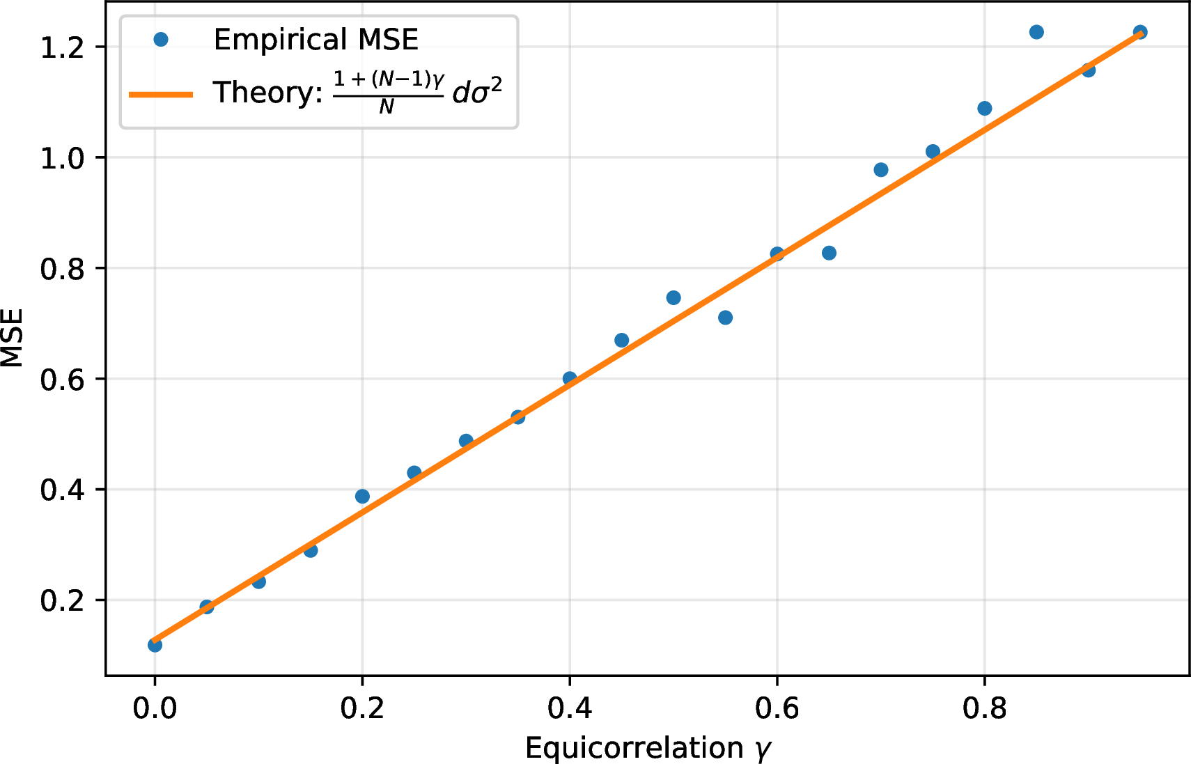
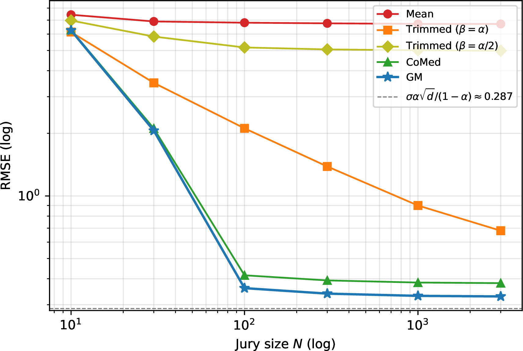
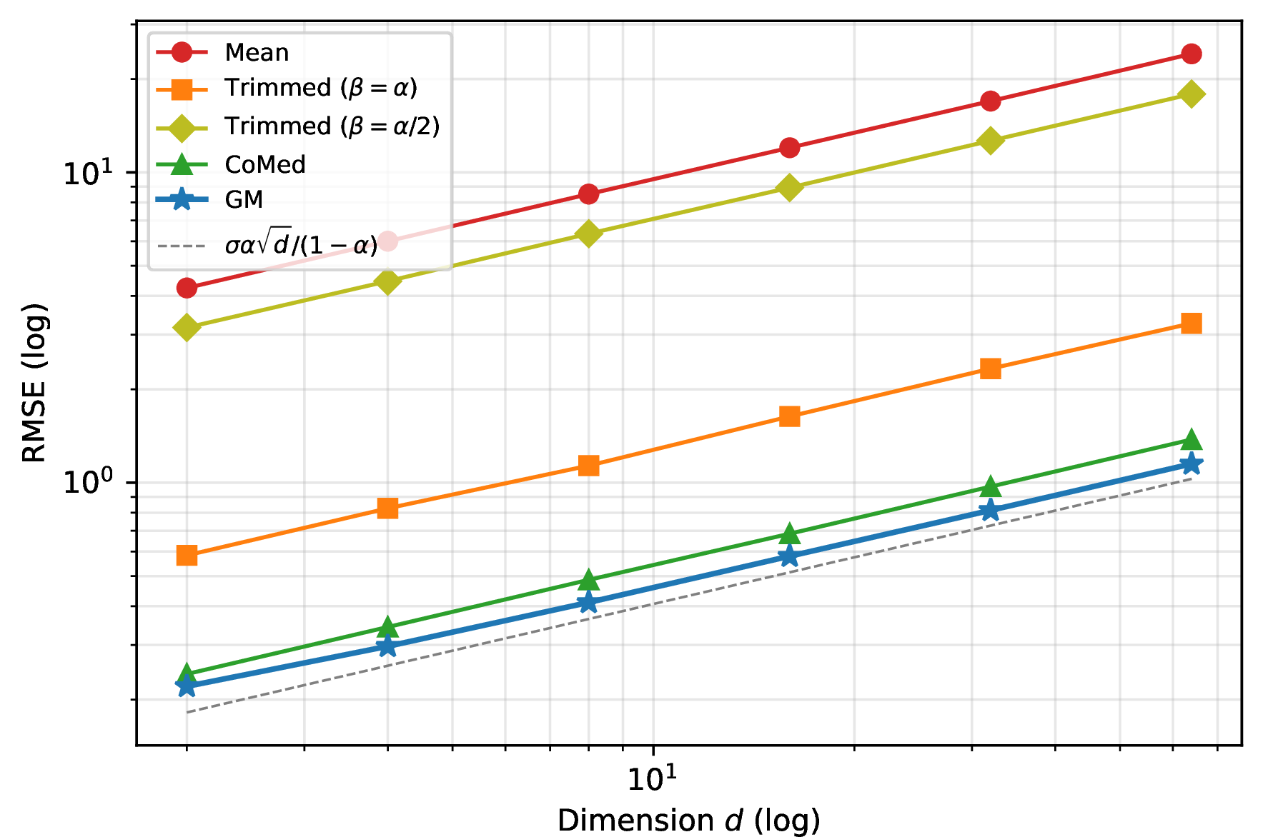
Figure 8: Theory validation. (a) Empirical MSE of the arithmetic mean for \(N{=}10\) equicorrelated clean Gaussian judges matches the closed-form prediction \(\tfrac{1+(N{-}1)\gamma}{N}\,d\sigma^{2}\) (Corollary 1) across the full range \(\gamma \in[0, 0.95]\); the effective jury size \(N_{\mathrm{eff}} = N/(1+(N{-}1)\gamma)\) saturates at \(1/\gamma\), motivating the three-judge committees of §6. (b) Under worst-case Huber contamination (\(\alpha{=}0.3\), \(\sigma{=}0.3\), \(d{=}5\), Dirac corruption at \({\mathbf{y}}^{\star}+10\,{\mathbf{1}}\)), the geometric median converges to the predicted breakdown floor \(\sigma\alpha\sqrt{d}/(1{-}\alpha) \approx 0.287\) (gray dashed) as \(N\) grows, matching Theorem 1; the arithmetic mean and under-trimmed mean (\(\beta{=}\alpha/2\)) plateau above the floor, confirming Proposition 2. (c) Holding \(N{=}1000\) fixed and sweeping the dimension, the geometric median tracks the predicted \(\sqrt{d}\) scaling of the cluster radius (Lemma 2) to within an absolute constant.. a — 1., b — 1., c — 2.
We bound \(\|\hat{{\mathbf{y}}}_{\mathrm{GM}} - {\mathbf{y}}^{\star}\|_{2}\) under our Huber model in two steps: a deterministic geometric lemma about the geometric median (Lemma 1, due to [@minsker2015geometric]), and a probabilistic lemma that controls the sub-Gaussian cluster radius (Lemma 2). Plugging the cluster radius into the geometric lemma yields Theorem 1, our finite-sample upper bound on RoPoLL. Full proofs are in Appendix 8.
Lemma 1 (Geometric Breakdown of GM). **([@minsker2015geometric], Lemma 2.1; building on [@lopuhaa1991breakdown].)* Let \(x_{1}, \ldots, x_{k} \in \mathbb{R}^{d}\) and let \(x_{*}\) be any minimizer of \(z \mapsto \sum_{j=1}^{k} \|z - x_{j}\|_{2}\) (a geometric median). Fix \(\alpha \in (0, 1/2)\), \(r > 0\), and \(z \in \mathbb{R}^{d}\). If \(|\{j : \|x_{j} - z\|_{2} \leq r\}| \geq (1-\alpha)k\), then \[\label{eq:gm95breakdown} \big\|x_{*} - z\big\|_{2} \;\leq\; C_{\alpha}\, r, \qquad C_{\alpha} \;\triangleq\; \frac{1-\alpha}{\sqrt{1-2\alpha}}.\tag{8}\] *
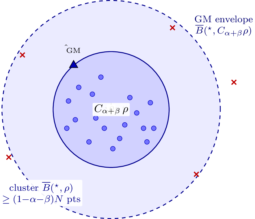
This is purely deterministic: a multiplicative bound between the geometric median and any target \(z\) in terms of how concentrated the inputs are around \(z\). The constant \(C_{\alpha}\) is sharp and diverges as \(\alpha \to 1/2\), matching the breakdown point of GM. 6 illustrates the geometric core of the proof: under the contradiction hypothesis \(\Delta = \|x_{*}-z\|_{2} > C_{\alpha}r\), the cluster ball subtends a narrow cone at \(x_{*}\), forcing the \((1{-}\alpha)k\) cluster points to lie inside it—and a balance of unit-vector subgradients (the first-order optimality condition for the geometric median) produces the contradiction.
Lemma 2 (Sub-Gaussian Cluster Radius). Under Assumptions 2–5, let \(\beta \in (0,\, 1/2 - \alpha)\) be a slack parameter. With probability at least \(1 - \exp(-N\beta^{2}/2)\), \[\label{eq:cluster95radius} \big|\big\{i \in [N] : \|\hat{{\mathbf{y}}}_{i} - {\mathbf{y}}^{\star}\|_{2} \leq \rho\big\}\big| \;\geq\; (1 - \alpha - \beta)\,N,\qquad{(8)}\] where the cluster radius is \[\label{eq:cluster95radius95rho} \rho \;=\; \sigma\!\left(C_{1}\sqrt{d} \;+\; \sqrt{\frac{1}{c}\,\log\!\frac{2(1-\alpha)}{\beta}}\right),\qquad{(9)}\] and \(C_{1}, c > 0\) are absolute constants (from the sub-Gaussian-norm tail bound, Step 1 of the proof in Appendix 8.6).
The slack \(\beta\) controls a trade-off: a larger \(\beta\) permits a smaller cluster radius \(\rho\) (since fewer competent samples need to be inside) but augments the effective contamination threshold from \(\alpha\) to \(\alpha + \beta\) in the geometric step.
Theorem 1 (RoPoLL Breakdown Bound under Huber Contamination). Under Assumptions 2–5, fix any slack \(\beta \in (0,\, 1/2 - \alpha)\). With probability at least \(1 - \exp(-N\beta^{2}/2)\), \[\label{eq:ropoll95bound} \big\|\hat{{\mathbf{y}}}_{\mathrm{GM}} - {\mathbf{y}}^{\star}\big\|_{2} \;\leq\; \underbrace{\frac{1 - \alpha - \beta}{\sqrt{1 - 2\alpha - 2\beta}}}_{C_{\alpha+\beta}} \;\cdot\; \underbrace{\sigma\!\left(C_{1}\sqrt{d} \;+\; \sqrt{\frac{1}{c}\log\!\frac{2(1-\alpha)}{\beta}}\right)}_{\rho}.\qquad{(10)}\]
The proof is a one-line combination: applying Lemma 1 with \(k = N\), \(z = {\mathbf{y}}^{\star}\), \(r = \rho\), and effective threshold \(\alpha' = \alpha + \beta < 1/2\), the count bound from Lemma 2 is exactly the hypothesis of Lemma 1, so the geometric lemma gives \(\|\hat{{\mathbf{y}}}_{\mathrm{GM}} - {\mathbf{y}}^{\star}\|_{2} \leq C_{\alpha+\beta}\,\rho\). Full details are in Appendix 8.7.
5.1.0.1 Interpretation.
The bound has two components. The geometric constant \(C_{\alpha+\beta}\) depends only on the contamination rate (and slack); it diverges as \(\alpha + \beta \to 1/2\), encoding the breakdown point. The cluster radius \(\rho\) depends only on the noise scale \(\sigma\) and the dimension \(d\); it does not shrink with \(N\). This reflects the breakdown-point character of plain GM: under arbitrary \(Q\) in the Huber class, the asymptotic-\(N\) floor is set by the cluster radius, not by sample averaging. The bound is distribution-free over the corruption class \(\{Q_{i}\}\). 5 illustrates the two-step geometry. For comparison with the matching minimax lower bound (Theorem 2), see §5.2.
5.1.0.2 Synthetic validation.
8 validates the i.i.d.theory on controlled synthetic data: panel (a) confirms the closed-form clean-jury MSE of Corollary 1; panel (b) shows the geometric median converging to the predicted breakdown floor \(\sigma\alpha\sqrt{d}/(1-\alpha)\) as \(N\) grows under worst-case Huber contamination, while PoLL stays above the floor (Proposition 2); panel (c) confirms the \(\sqrt{d}\) scaling of the cluster radius \(\rho\) (Lemma 2) at fixed \(N\).
5.1.0.3 Beyond i.i.d.: equicorrelated juries.
Theorem 1 assumes conditional independence (Assumption 3). Real LLM juries trained on overlapping corpora violate this: inter-judge correlation \(\bar\gamma \in [0.3, 0.7]\) is typical ([fig:corpus_judge_corr,sec:appendix_dataset_correlation]). We close §5.1 by extending Theorem 1 to this regime: the breakdown structure (\(C_{\alpha+\beta}\) and \(\rho\)) survives unchanged; only the high-probability event weakens, from exponential in \(N\) to polynomial in the effective jury size \(N_{\mathrm{eff}} = N/(1+(N-1)\bar\gamma_{W})\) familiar from Corollary 1.
The proof replaces the Hoeffding step of Lemma 2 with a Chebyshev bound on \(\sum_{i}W_{i}\) under the bounded-covariance hypothesis; the cluster radius \(\rho\) and the geometric constant \(C_{\alpha+\beta}\) are unchanged because Lemma 1 is purely deterministic. The hypothesis is on the indicator correlation \(\bar\gamma_{W}\), which we estimate directly from the empirical co-incidence of cluster events \(\{W_{i} = 1\}\) on our \(13\)-judge experimental panels ([sec:appendix_gamma_W,tab:empirical_gamma_W]): across three cluster-radius calibrations (50th/70th/90th percentiles of pooled per-sample deviations), \(\bar\gamma_{W} \in [0.45, 0.53]\) on HelpSteer-2 and UltraFeedback, in line with the inter-judge score correlations \(\bar\gamma \in [0.49, 0.71]\) of 15. At \(N{=}3\) this gives \(N_{\mathrm{eff}} \in [1.45, 1.58]\); the breakdown floor and geometric constant are unaffected, and the high-probability event remains non-trivial for the moderate slack \(\beta\) used in practice. Full details are in Appendix 8.8.
5.2 Minimax Lower Bound↩︎
We close the section with a matching information-theoretic minimax lower bound that exposes a \(\sqrt{d}\) statistical–computational gap: RoPoLL is rate-optimal up to a dimensional constant on the breakdown floor, the price for \(O(Nd\log(1/{\epsilon}))\) tractability via the Weiszfeld iteration. No estimator can do better on the parametric variance term; the breakdown floor, in turn, is matched up to a dimensional constant only by the (intractable) Tukey halfspace median.
Theorem 2 (Minimax Lower Bound). Under the same assumptions as Theorem 1, \[\label{eq:minimax95body} \inf_{\hat{{\mathbf{y}}}}\;\sup_{F \in {\mathcal{F}}_{\alpha,\sigma}}\; \mathbb{E}_{F}\!\left[\|\hat{{\mathbf{y}}} - {\mathbf{y}}^{\star}\|_{2}\right] \;\geq\; c\sigma\!\left(\sqrt{d/N} \;+\; \frac{\alpha}{1-\alpha}\right),\qquad{(12)}\] where the infimum is over all measurable estimators of the form \(\hat{{\mathbf{y}}}(\hat{{\mathbf{y}}}_{1}, \ldots, \hat{{\mathbf{y}}}_{N})\), \({\mathcal{F}}_{\alpha,\sigma}\) is the class of joint distributions consistent with Assumptions 2, 3, 4, and 5, and \(c > 0\) is a universal constant.
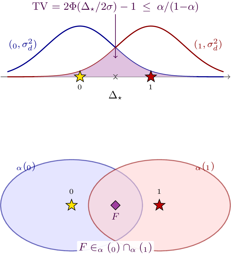
Proof sketch. We use Le Cam’s two-point method. For the \(\sqrt{d/N}\) term, set \(\alpha = 0\) and pit two clean Gaussian hypotheses \({\mathbf{y}}_{0} = {\mathbf{0}}\) vs. \({\mathbf{y}}_{1} = \Delta\,{\mathbf{e}}_{1}\) with \(\Delta = c_{1}\sigma\sqrt{d/N}\); the standard Pinsker-plus-tensorisation calculation gives \(\mathrm{TV}(F_{0}^{\otimes N}, F_{1}^{\otimes N}) \leq 1/2\). For the \(\alpha/(1-\alpha)\) term, we exploit the modulus of continuity of the Huber neighborhood: the contamination class \({\mathcal{F}}_{\alpha}({\mathbf{y}}) = \{(1-\alpha){\mathcal{N}}({\mathbf{y}}, \sigma^{2}{\mathbf{I}}_{d}) + \alpha Q\}\) contains a common distribution at two centers \({\mathbf{y}}_{0}, {\mathbf{y}}_{1}\) whenever \(\|{\mathcal{N}}({\mathbf{y}}_{0}, \sigma^{2}{\mathbf{I}}_{d}) - {\mathcal{N}}({\mathbf{y}}_{1}, \sigma^{2}{\mathbf{I}}_{d})\|_{\mathrm{TV}} \leq \alpha/(1-\alpha)\), since both \((1-\alpha){\mathcal{N}}({\mathbf{y}}_{0}, \sigma^{2}{\mathbf{I}}_{d})\) and \((1-\alpha){\mathcal{N}}({\mathbf{y}}_{1}, \sigma^{2}{\mathbf{I}}_{d})\) are then dominated componentwise by a single probability measure. TV between two equal-covariance Gaussians at separation \(\Delta\) is \(2\Phi(\Delta/(2\sigma)) - 1\) (dimension-free), so the largest indistinguishable separation is \(\Delta_{\star} = 2\sigma\Phi^{-1}\!\left(\tfrac{1}{2} + \tfrac{\alpha}{2(1-\alpha)}\right) \geq \sqrt{2\pi}\,\sigma\alpha/(1-\alpha)\). Le Cam then gives error at least \(\Delta_{\star}/4\). The full proof is in Appendix 8.9. ◻
7 illustrates the modulus-of-continuity construction: when the two Gaussians at \({\mathbf{y}}_{0}\) and \({\mathbf{y}}_{1}\) are TV-close enough, their Huber neighborhoods overlap at a common distribution \(F\) that is consistent with both truths—making the two centers indistinguishable from any number of i.i.d.samples.
5.2.0.1 Comparison with the upper bound.
Theorems 1 and 2 match exactly on the parametric rate \(\sigma\sqrt{d/N}\). On the breakdown floor they differ by a \(\sqrt{d}\) factor: the upper bound scales as \(C_{\alpha}\sigma\sqrt{d}\) while the lower bound scales as \(\sigma\alpha/(1-\alpha)\). This is not a slack in the analysis but a real statistical–computational gap. The minimax-optimal estimator on the breakdown floor is the Tukey halfspace median [@tukey1975mathematics; @donoho1992breakdown], whose exact computation is NP-hard for \(d \geq 3\) [@johnson1978densest; @aloupis2006geometric]; the smoothed-depth estimator of [@chen2018robust] matches the \(\sigma\alpha\) floor in sub-exponential time. The geometric median is the polynomial-time alternative: it shares the optimal \(1/2\) breakdown point but pays a \(\sqrt{d}\) price for \(O(Nd\log(1/{\epsilon}))\) tractability via the Weiszfeld iteration (§4.3). For LLM juries the trade is favourable: \(d\) is small (1–5 in our benchmarks) so the \(\sqrt{d}\) overhead is at most \(\sim 2.2\times\), and at \(N = 3\) the variance term \(\sigma\sqrt{d/N}\) dominates the breakdown floor on every regime we test (§6.6). RoPoLL is therefore an efficient robust estimator, matching the minimax breakdown point at the small price of a dimensional constant on the contamination floor.
5.2.0.2 Scope of the i.i.d.assumptions.
Theorems 1 and 2 are stated under the i.i.d.baseline (Asm 3, identical \(\sigma_{i}\)). Lemma 3 relaxes independence to equicorrelation, covering the inter-judge correlation \(\bar\gamma \in [0.3, 0.7]\) measured in our experiments. Two further deviations remain out of scope: per-judge heterogeneity (\(\sigma_{i}, \alpha_{i}\) varying across the \(4\)–\(675\) B parameter range) and explicit dependence by design (peer-rank discussion [@li2024prd], multi-agent debate [@chan2024chateval], judge networks [@zhang2024wider]). The empirical evaluation in §6 holds these axes fixed and isolates the effect of contamination type and rate; the heterogeneous-jury extension—together with side information such as per-judge calibration on a labeled validation slice—is the subject of follow-up work.
6 Experiments↩︎
We evaluate RoPoLL against PoLL (the arithmetic-mean baseline of [@verga2024replacing]) and the coordinate-wise Median on three reward-model benchmarks under a per-case corruption pipeline that exposes the corruption-type dependence predicted by Theorem 1 and Example 1.

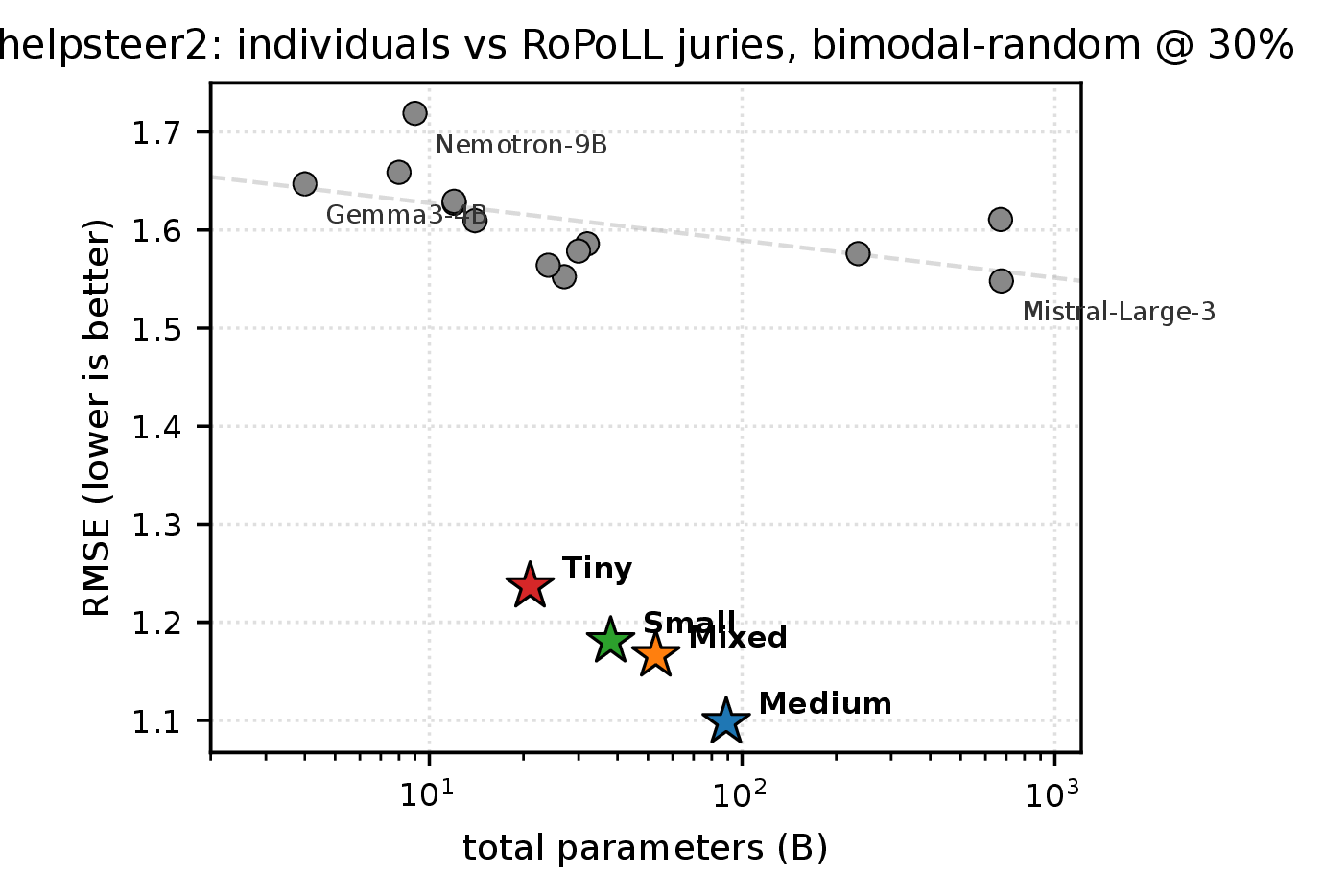
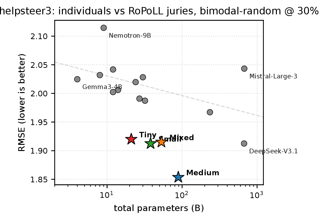
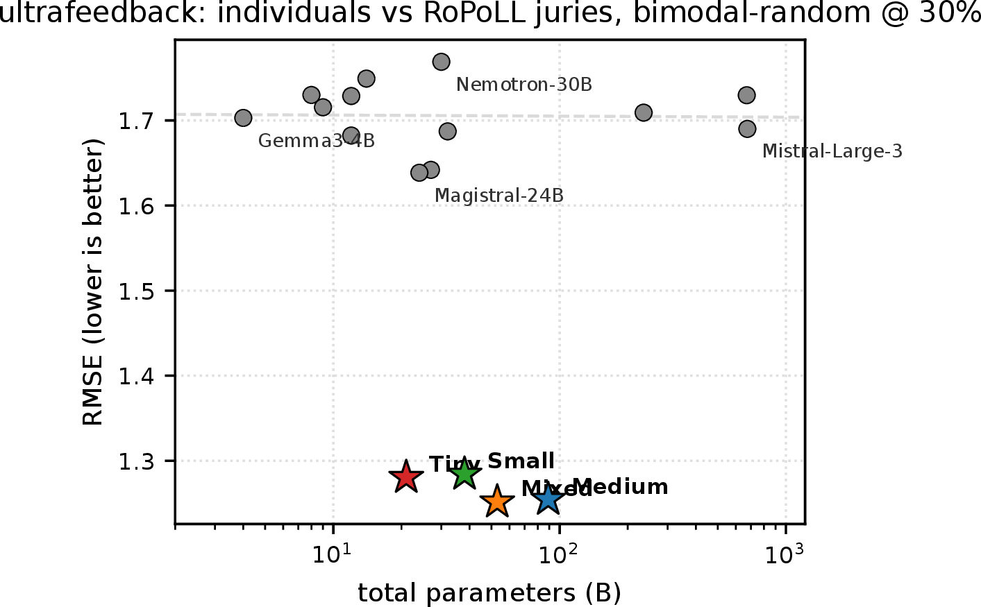
Figure 9: Parameter efficiency of RoPoLL juries vs. individual judges under bimodal-random corruption at \(r = 30\%\). RMSE vs.parameter count (log
scale) for each dataset; gray circles are the 13 individual open-weight judges (four anchors labelled), dashed line is their log-linear scaling fit, and coloured stars mark the four RoPoLL juries (Medium/Mixed/Small/Tiny) at
their aggregate parameter budget—all evaluated under identical \(30\%\) per-case corruption. bimodal-random drives each coordinate of a corrupted score independently to an extremum, instantiating the
cross-dimensional failure mode of Example 1; clean-baseline and zeros counterparts are in [fig:p5_jury_vs_individual_clean,fig:p3_hero_rmse_zeros].. b — HelpSteer 2, c — HelpSteer 3, d — UltraFeedback
6.1 Setup↩︎
6.1.0.1 Datasets.
We use three popular reward model benchmarks with complementary ground-truth sources. HelpSteer 2 [@wang2024helpsteer2] contributes \(1{,}000\) samples drawn uniformly at random from the validation split, each rated on a \(0\)–\(4\) Likert scale across five attributes (helpfulness, correctness,
coherence, complexity, verbosity) by trained human annotators. HelpSteer 3 [@wang-etal-2025-helpsteer3] contributes its full \(2{,}017\)-sample multilingual validation split; the native chosen-vs-rejected preference is converted to a scalar overall_preference target on \([-4, 4]\) by re-scoring both
responses on the HelpSteer 2 rubric and taking the signed difference. UltraFeedback [@cui2024ultrafeedback] contributes \(1{,}000\) samples
scored on a \(1\)–\(5\) scale across four attributes (helpfulness, honesty, instruction following, truthfulness) using GPT-4 as the reference annotator.
6.1.0.2 Judges and juries.
We score every sample with \(13\) open-weight judges spanning \(4\)–\(675\) B parameters at temperature \(0\) under a shared structured rubric: Mistral-Large-3 (\(675\) B), DeepSeek-V3.1 (\(671\) B), Qwen3-235B, Qwen3-32B, Nemotron-30B, Gemma-27B, Magistral-Small (\(24\) B), Ministral-14B, Gemma-12B, Nemotron-12B, Nemotron-9B, Ministral-8B, and Gemma-4B. From these we curate four three-judge committees that trade size against compute: Medium \(\approx 89\) B (Qwen3-32B, Nemotron-30B, Gemma-27B), Mixed \(\approx 53\) B (Qwen3-32B, Gemma-12B, Nemotron-9B), Small \(\approx 38\) B (Ministral-14B, Gemma-12B, Nemotron-12B), and Tiny \(\approx 21\) B (Nemotron-9B, Ministral-8B, Gemma-4B). The choice of \(N = 3\) is not arbitrary: under the equicorrelated jury model of Corollary 1 the effective jury size \(N_{\mathrm{eff}} = N/(1 + (N-1)\gamma)\) saturates at \(1/\gamma\) as \(N \to \infty\), so for the moderate inter-judge correlation \(\gamma \in [0.3, 0.5]\) characteristic of diverse but non-orthogonal LLM backbones, \(N_{\mathrm{eff}}\) saturates already at \(N \approx 2\)–\(3\) (8 (a) of 8, §5.1)—a prediction corroborated by the empirical diminishing-returns knee at \(N = 3\) in 12. We compare PoLL (arithmetic mean), the coordinate-wise Median, and RoPoLL (Algorithm 4) on these committees; all three operate on the same three (possibly corrupted) score vectors per sample.
6.1.0.3 Per-case corruption protocol.
Rather than injecting extra adversarial judges into a fixed pool, we hold the jury size at three and corrupt individual (sample, judge) cells at a per-case rate \(r \in \{0\%, 10\%, 20\%, 30\%, 40\%, 50\%\}\),
matching the realistic failure pattern in which a judge occasionally emits a bad score on a specific input. The sweep range is calibrated against the natural-failure characterization of 2 (§3.4): naturally-occurring rates span \(0.59\%\) on HelpSteer 2 to \(33\%\) on HelpSteer 3 multilingual, so \(r \in [0, 50\%]\)
covers the natural regime and stress-tests beyond. We consider four corruption types covering distinct adversarial regimes: (i) zeros, where every corrupted slot is replaced by \({\mathbf{0}}\) (the
parser-failure fallback); (ii) inverted, where corrupted slots are replaced by \(K \cdot {\mathbf{1}}- {\mathbf{y}}^{\star}\) (the worst-case anti-correlated Byzantine attack); (iii)
bimodal-random, where each coordinate of the corrupted slot is independently set to \(0\) or \(K\) with equal probability (the cross-dimensional failure mode of Example 1); and (iv) cauchy-far, where each corrupted slot is drawn as \({\mathbf{y}}^{\star} + 10 +
2(s_{\max}\!-\!s_{\min})\!\cdot\!{\mathbf{t}}\) with \({\mathbf{t}}\) component-wise standard Cauchy (a biased heavy-tailed Byzantine attack with undefined mean and variance). Pre-existing parser failures from real
judges are dropped at \(r = 0\%\) and replaced with adversarial vectors at \(r > 0\%\), so the effective observed corruption rate at \(r > 0\) is \(f + (1 - f)\,r\) with \(f\) the naturally occurring parser-failure rate. We report RMSE against the reference labels; per-judge calibration breakdowns (MAE, mean bias) on the UltraFeedback
rubric dimensions are in Appendix 9.2.
6.2 Heavy-Tailed Corruption↩︎
The cauchy-far attack is the empirical analogue of the adversarial choice in Proposition 2: each corrupted slot has an unbounded first moment, and a
single contaminated judge can in principle drag PoLL by an arbitrary amount. The teaser (1, queued in §1) confirms this empirically. On the Medium jury, PoLL’s RMSE exceeds RoPoLL’s by one to three orders of magnitude at every \(r \geq 10\%\) on all three benchmarks. The
largest gap occurs on HelpSteer 2 at \(r = 40\%\), where PoLL’s RMSE reaches \(\approx 4{,}951\) while RoPoLL holds at \(\approx 9.2\)—a ratio of \(\approx 540\times\). The coordinate-wise Median is competitive with RoPoLL here (full three-method
comparison in 13, §6.6): under heavy-tailed Byzantine attacks any robust aggregator beats the mean, exactly as the theory predicts.
6.3 Cross-Dimensional Corruption↩︎
The bimodal-random attack drives each coordinate of a corrupted score independently to an extremum—each corrupted score is plausible per coordinate but jointly anomalous, the failure mode predicted by Example 1. 9 plots, for each benchmark, the \(13\) individual judges (gray circles) against their parameter count
alongside the four RoPoLL committees (coloured stars) at their aggregate parameter count, both evaluated under identical \(30\%\) bimodal-random corruption. On HelpSteer 2 and
UltraFeedback, all four RoPoLL committees sit visibly below the individual-at-30% scaling trend. The headline number: on HelpSteer 2, the Small committee at \(38\) B reaches RMSE \(= 1.18\), beating Mistral-Large-3’s \(1.55\) at \(675\) B—a \(1.31\times\) accuracy advantage at \(18\times\) fewer parameters. On the harder HelpSteer 3 (signed-preference target), the Medium committee at \(89\) B still matches DeepSeek-V3.1 (\(671\) B) at RMSE \(= 1.85\).
6.3.0.1 Compute-matched comparison.
The single-judge-vs-committee framing above understates the case for robust aggregation, because any 3-judge committee (\(114\) B–\(267\) B forward-pass compute) beats a single
\(675\) B judge at evaluation cost. The fair compute-matched comparison is RoPoLL versus PoLL on the same committee. On the Small
committee at \(30\%\) bimodal-random, RoPoLL (RMSE \(1.18\)) beats PoLL (RMSE \(\approx
1.45\)) on the same three judges by \(\approx 19\%\) at identical inference cost (13, full grid): the parameter-efficiency advantage holds because the geometric
median’s joint-distance objective extracts more signal from the same forward passes than PoLL. Robust aggregation, not the ensemble itself, is what delivers the win.
6.4 Bounded Mean-Preserving Corruptions: Zeros and Inverted↩︎

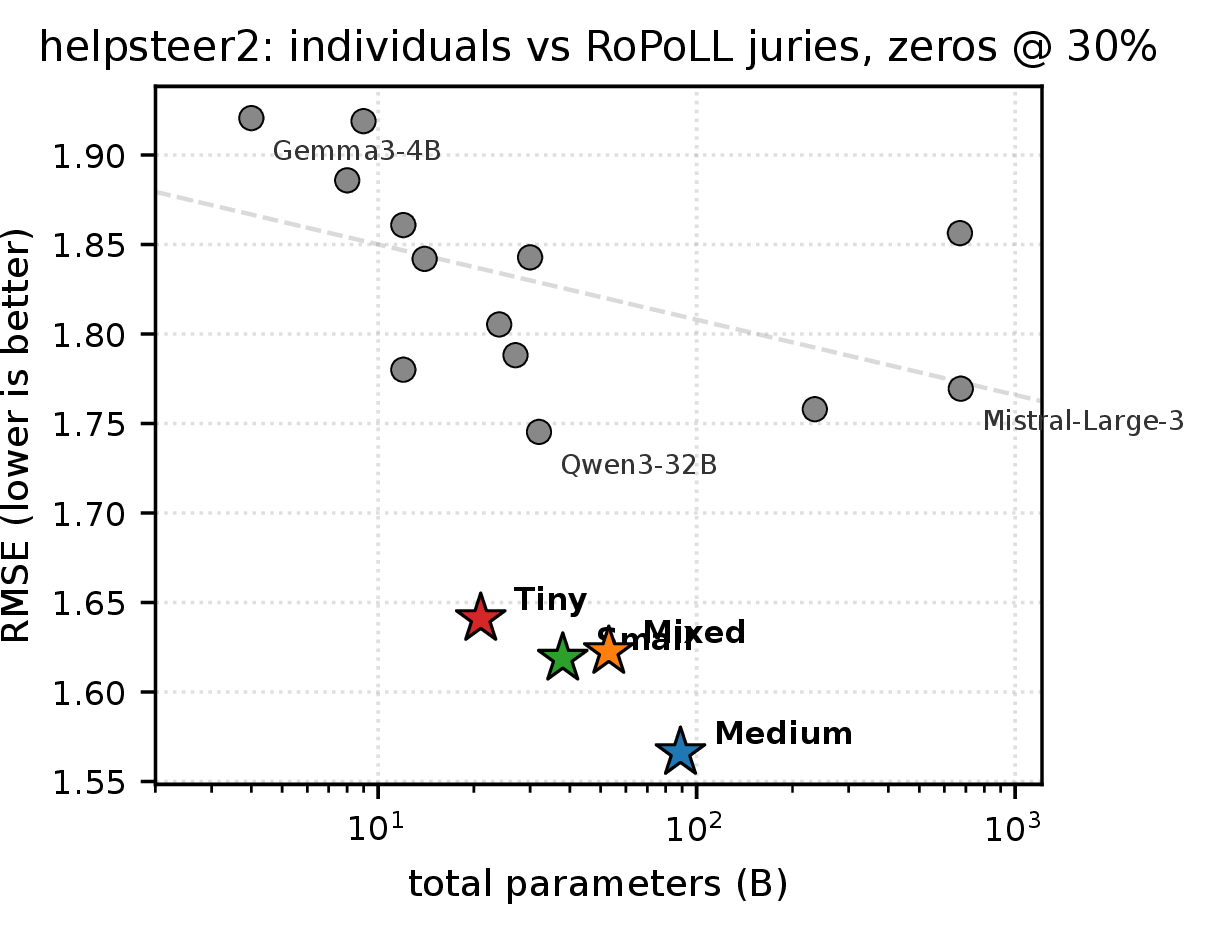
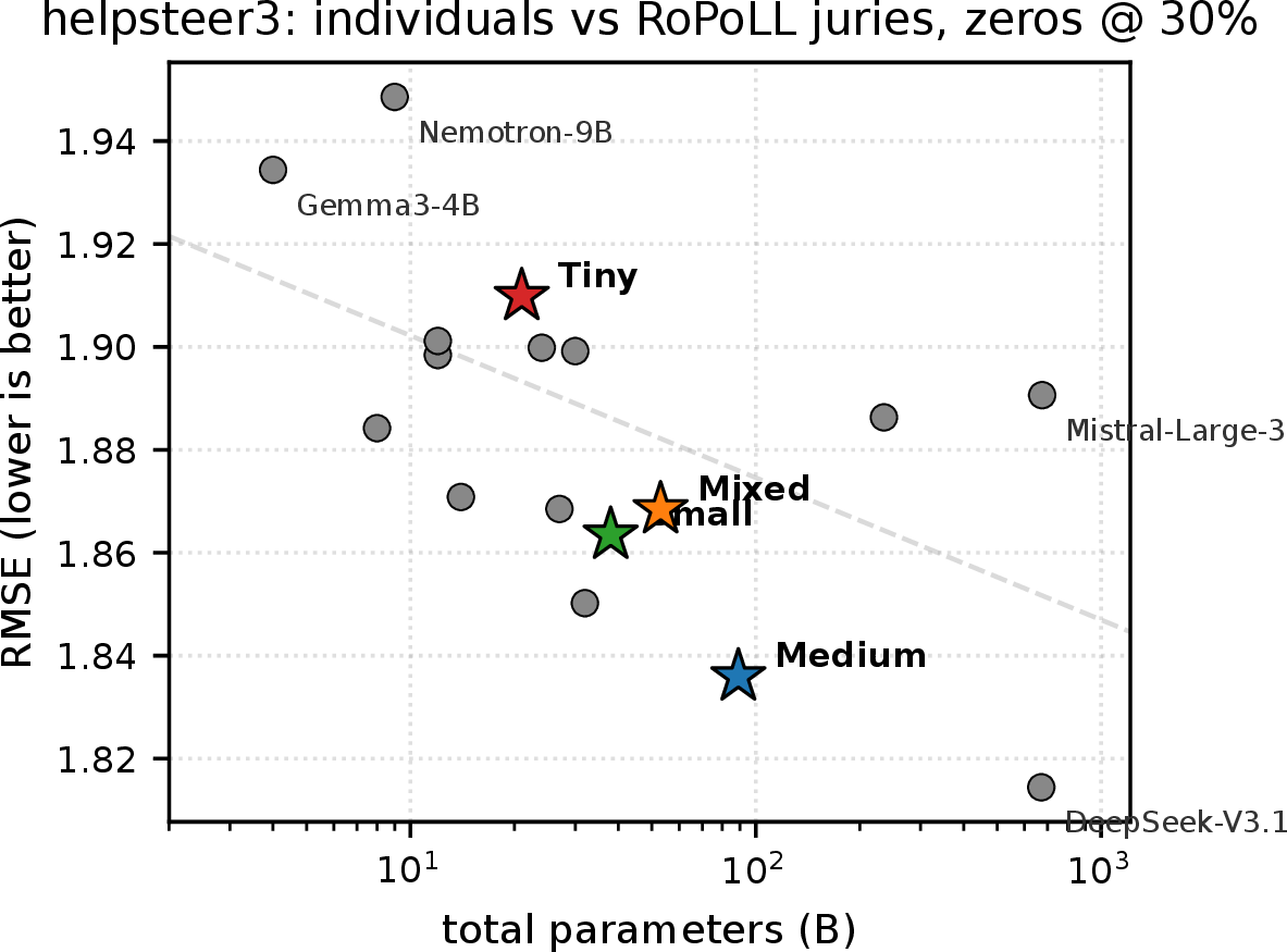
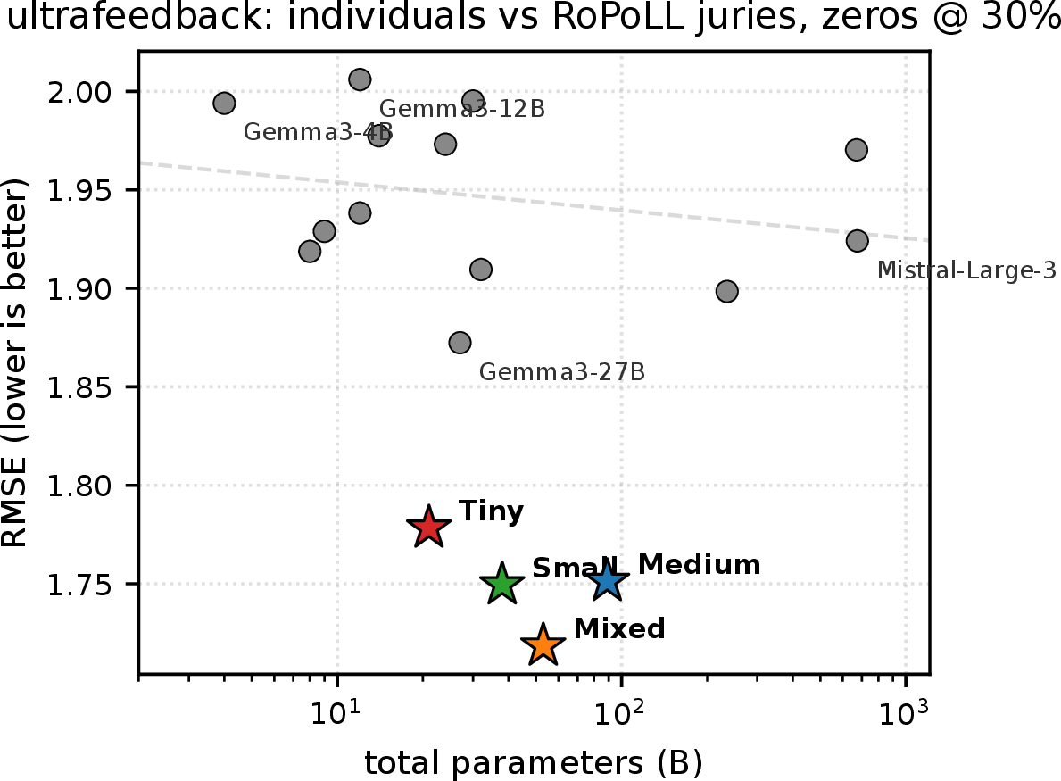
Figure 10: Parameter efficiency of RoPoLL juries vs. individual judges under zeros corruption at \(r = 30\%\). RMSE vs.parameter count (log scale)
for each dataset; gray circles are the 13 individual open-weight judges (four anchors labelled), dashed line is their log-linear scaling fit, and coloured stars mark the four RoPoLL juries at their aggregate parameter budget,
all under identical \(30\%\) per-case corruption. zeros replaces each corrupted slot with the parser-fallback vector \({\mathbf{0}}\); the direct RoPoLL vs.PoLL contrast is deferred to 13.. b — HelpSteer 2, c — HelpSteer 3, d — UltraFeedback
The zeros and inverted attacks place corrupted scores at fixed bounded points on the score scale. On a bounded scale PoLL is mean-preserving under uniform-rate corruption when the
corrupted point happens to lie at the scale midpoint—an empirical accident, not a property of the mean as an estimator—which makes these the regimes where RoPoLL and PoLL should be hardest to
separate. 10 plots the parameter-efficiency view under \(30\%\) zeros corruption on the same axes as 9. The
headline: even in this favourable-to-the-mean regime, all four RoPoLL committees sit at or below the individual-at-30% scaling line on every benchmark, and the gap to PoLL remains positive but
small (\(\leq 0.3\) RMSE for the Medium jury across the full corruption sweep—see 13). RoPoLL is therefore not a
universal replacement for the mean: when the corruption is bounded and happens to be mean-preserving, the two are within an insurance premium of each other. The argument for RoPoLL as a default is that the practitioner does
not get to choose which regime the next corruption falls into.
6.5 Clean-Baseline Parameter Efficiency↩︎
![Figure 11: Parameter efficiency at the clean baseline (r = 0\%). RMSE vs.parameter count (log scale) for each dataset; gray circles are the 13 individual open-weight judges, dashed line is their log-linear scaling fit, and coloured stars mark the four RoPoLL juries at their aggregate parameter budget. Clean counterpart of [fig:p2_bimodal_ropoll_hero,fig:p3_hero_rmse_zeros].](/article/2606.30931/assets/param_efficiency_jury/paper/p5_jury_vs_individual_clean.png "fig:")
A natural concern about a robust aggregator is that the robustness costs accuracy in the absence of corruption. Theorem 1 predicts a small insurance premium at \(\alpha = 0\) (the geometric constant \(C_{\beta} \to 1\) as \(\beta \to 0\)); 11 cashes this empirically by plotting the four RoPoLL committees against the \(13\)-judge individual scaling line at \(r = 0\%\). The Medium, Mixed, and Small committees sit below the individual scaling line on every benchmark; Tiny is roughly on-trend. The clean-case insurance premium is at most \(+6.4\%\) relative RMSE across the full grid (median \(+0.9\%\)), so the cost of using RoPoLL when corruption happens to be absent is a small fraction of the gains it delivers when corruption is present.
6.6 Jury-Size Ablation and Corruption-Type Dependence↩︎
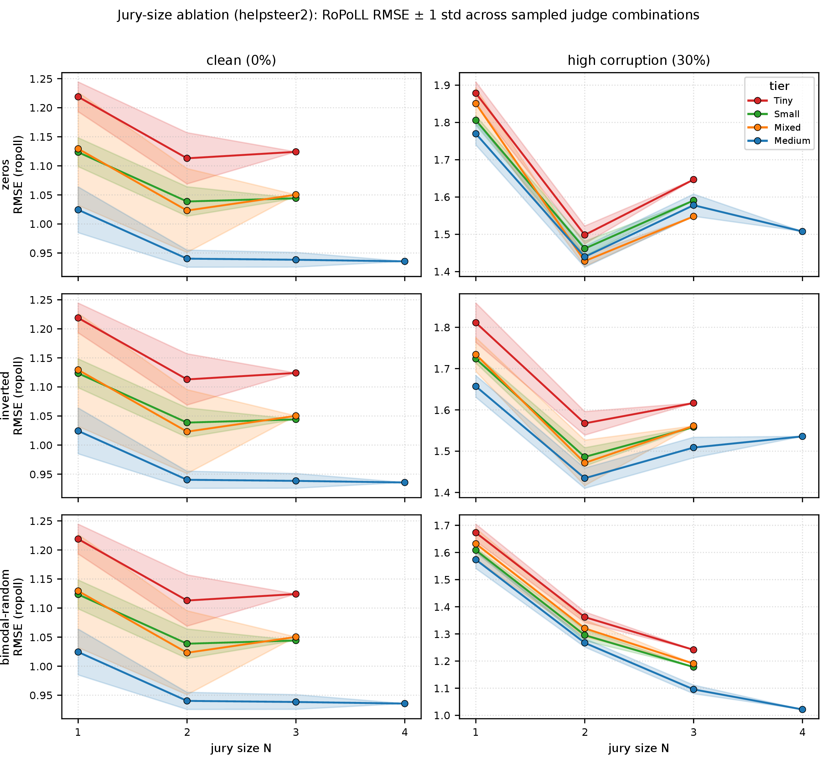
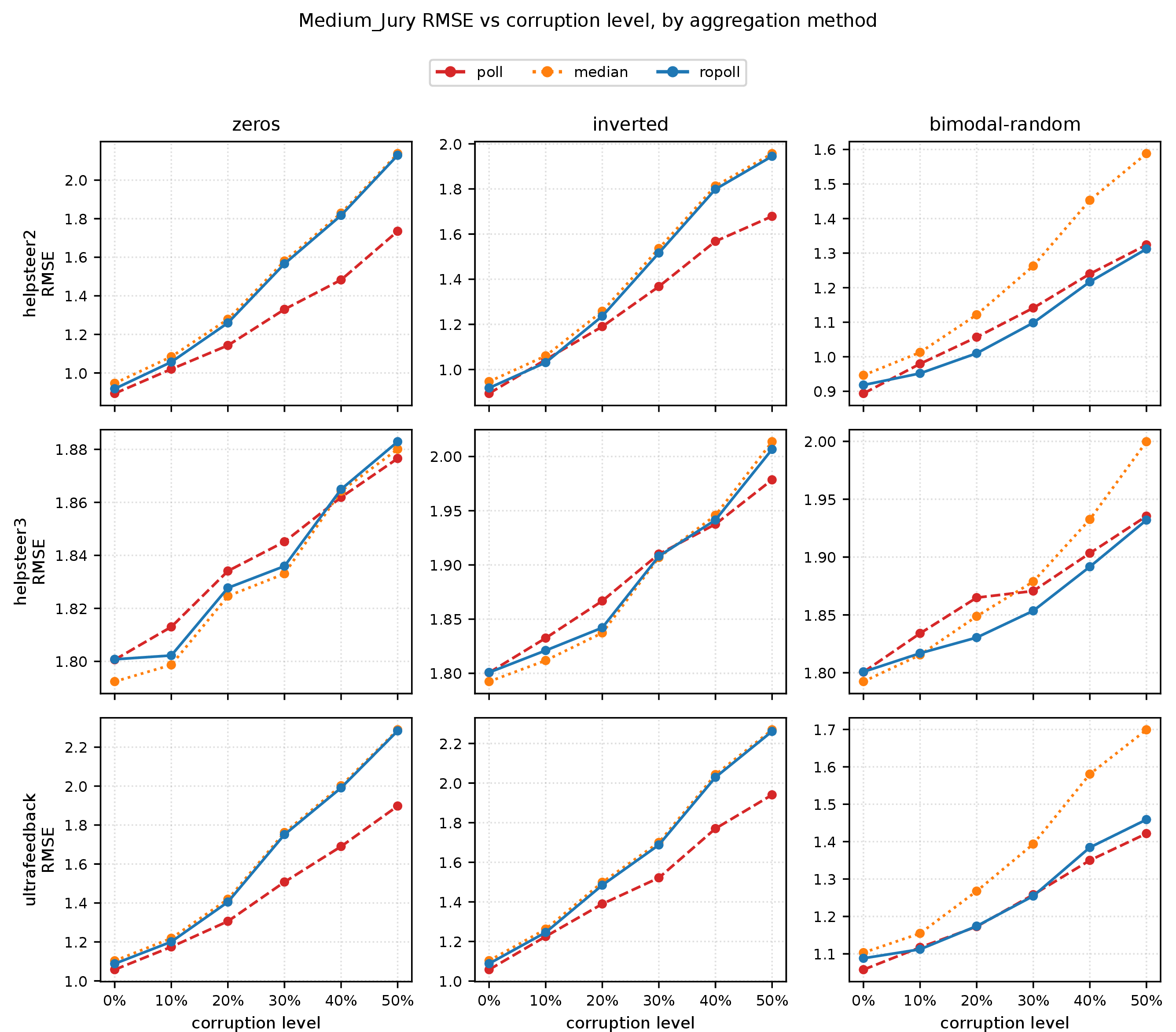
Two practical questions remain: how many judges does RoPoLL actually need, and is the geometric median always the right choice? 12 answers the first by sweeping the jury size \(N \in \{1, 2, 3, 4\}\) across the four committee tiers under three corruption types at the clean baseline (\(r = 0\%\), left column) and under heavy contamination (\(r = 30\%\), right column). 13 answers the second by reporting the full three-method PoLL/Median/RoPoLL comparison across every (dataset, corruption type, rate) cell.
6.6.0.1 Jury ablation.
RMSE drops sharply from \(N = 1\) to \(N = 3\) and levels off thereafter on every tier and corruption type, both clean and at \(30\%\) contamination; the marginal benefit of a fourth judge falls within the standard-deviation band, confirming the Corollary 1 prediction that the three-judge committees sit at the knee of the cost–accuracy frontier.
6.6.0.2 Corruption-type ablation.
Under zeros and inverted PoLL is mean-preserving on the bounded score scale and tracks RoPoLL within \(\pm 0.3\) RMSE; under
bimodal-random mean-preservation fails and RoPoLL stays below PoLL at every \(r \geq 10\%\); under cauchy-far the gap reaches one to
three orders of magnitude (see 13). The coordinate-wise Median tracks RoPoLL closely on heavy-tailed and bounded-symmetric corruptions but lags RoPoLL on bimodal-random, where the cross-dimensional structure (Example 1) is invisible to a per-coordinate median. At the clean
baseline, RoPoLL pays a small insurance premium (\(+0.01\%\) to \(+6.4\%\) relative RMSE). RoPoLL is a robust default
for high-penalty regimes.
6.7 Noisy-GT Control: Systematic Bias, Not Imprecision↩︎
A natural concern about robust aggregation is that the “insurance premium” might be paid on a phantom—if real judge failures are imprecise but unbiased rather than systematically wrong, robustness machinery is unnecessary. We test this directly with a Noisy-GT adversary that injects \(\hat{{\mathbf{y}}}_{\mathrm{noisy}} = \mathrm{clip}({\mathbf{y}}^{\star} + \boldsymbol{{\epsilon}}, 0, K)\) with \(\boldsymbol{{\epsilon}} \sim {\mathcal{N}}({\mathbf{0}}, 0.8^{2}{\mathbf{I}})\) in place of the adversarial vectors of §6.1. Empirically, all three aggregators improve as the Noisy-GT injection rate increases on both HelpSteer 2 and UltraFeedback, with PoLL slightly preferred (because averaging unbiased noise is statistically optimal under Gaussian errors). This rules out the most obvious confound: the RoPoLL premium reported in §§6.2–6.4 is paid against biased contamination, not imprecision. The full per-model and per-dimension breakdowns supporting this control are in Appendix 9.2.
6.8 Released Corpus↩︎
To support reproduction and follow-up work, we release the full \(13\)-judge \(\times\) three-benchmark output corpus that drives every figure in this section. For each \((\mathrm{judge},\,\mathrm{sample})\) cell the corpus contains the parsed score vector \(\hat{{\mathbf{y}}}_{f}(x) \in \mathbb{R}^{d}\) produced by the deterministic parser \(\phi\) (Definition 4), the per-call latency, and the reference label \({\mathbf{y}}^{\mathrm{ref}}_{j}\) (Definition 2); parser-failure cells are recorded as the all-zeros fallback vector. The corpus totals approximately \(28\mathrm{K}\) scored \((\mathrm{judge},\,\mathrm{sample})\) cells (Table 2), enabling exact reproduction of every reported figure without re-running the inference cost.
| Dataset | \(N_{\mathrm{samp}}\) | \(|J|\) | \(d\) | \(\bar f\) | \(f_{\max}\) | \(s_{\min}\) | \(s_{\max}\) |
|---|---|---|---|---|---|---|---|
| HelpSteer 2 | 1000 | 13 | 5 | 0.6% | 2.4% | \(-1.0\) | \(4.0\) |
| UltraFeedback | 1000 | 13 | 4 | 0.0% | 0.0% | \(1.0\) | \(5.0\) |
| HelpSteer 3 | 100 | 16 | 1 | 6.0% | 33.0% | \(-3.8\) | \(2.6\) |
4pt
6.8.0.1 Per-attribute score distributions.
14 plots the score distributions per attribute (per-dataset). HelpSteer 2 and UltraFeedback have substantial mass at the score extremes (parser fallback at \(0\); sycophantic
judges concentrating at the maximum), motivating the zeros and inverted corruption types used in §6. HelpSteer 3, which reduces a five-attribute pair of responses to a single signed-preference
scalar, is well-centered on \(0\) with light tails, consistent with the cancellation of per-attribute biases under the signed-difference reduction.
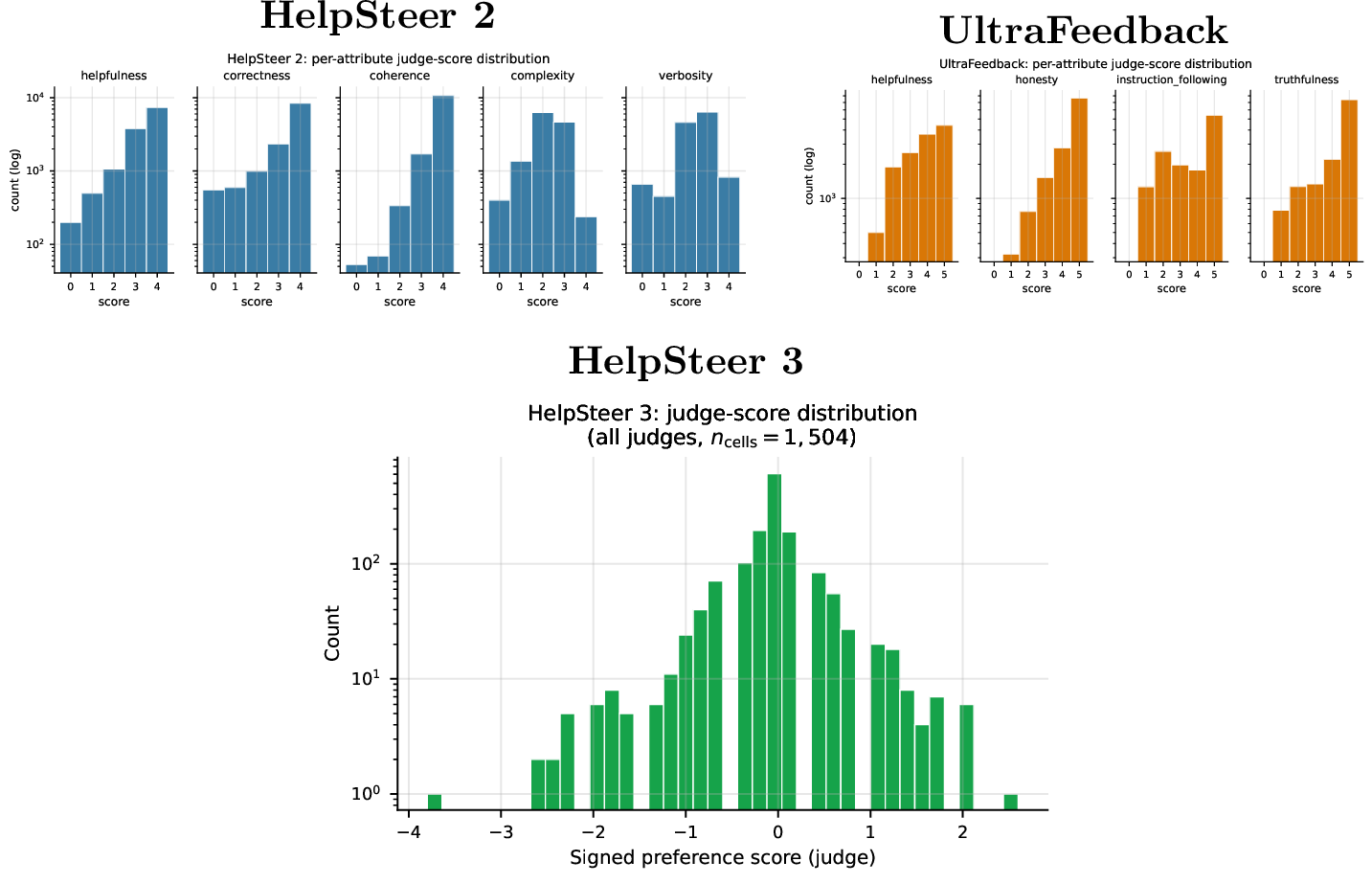
6.9 Inter-Judge Correlation Structure↩︎
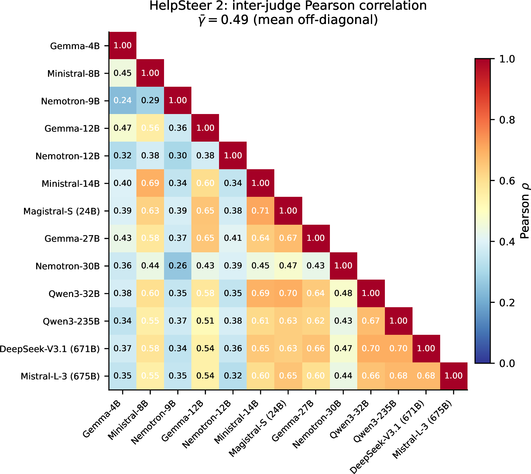
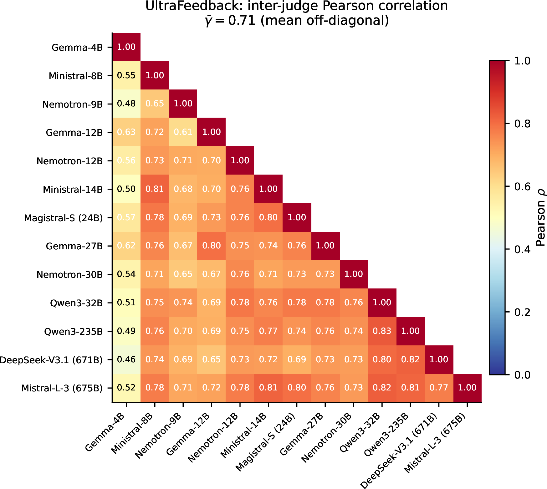
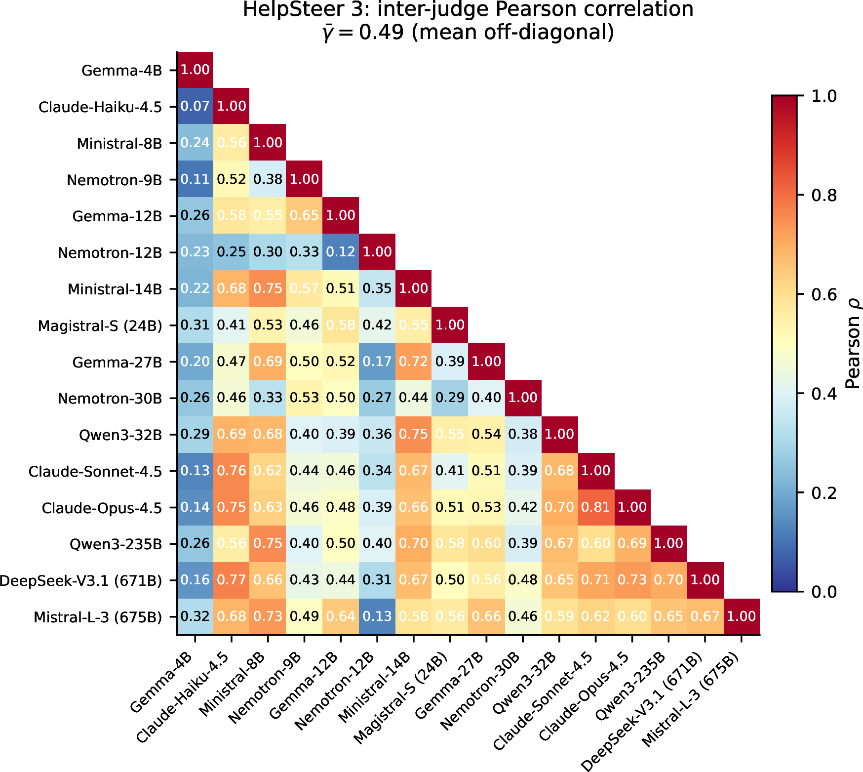
Figure 15: Inter-judge Pearson correlation heatmaps (lower-triangle, annotated). Pairwise correlations averaged over evaluation attributes; cells labelled with their numeric value. Empirical mean off-diagonal correlations: \(\bar\gamma_{\mathrm{HS2}} = 0.49\), \(\bar\gamma_{\mathrm{UF}} = 0.71\), \(\bar\gamma_{\mathrm{HS3}} = 0.49\). These values support the \(\gamma \in[0.3, 0.5]\) assumption used in §6.1 to motivate three-judge committees via Corollary 1; the higher \(\bar\gamma_{\mathrm{UF}}\) explains the smaller RoPoLL/PoLL gap observed on UltraFeedback..
15 shows the pairwise Pearson correlation between every judge pair in the \(13\)-judge pool, averaged over attributes. Empirical mean off-diagonal correlations are \(\bar\gamma_{\mathrm{HS2}} = 0.49\), \(\bar\gamma_{\mathrm{HS3}} = 0.49\), and \(\bar\gamma_{\mathrm{UF}} = 0.71\). These directly support the assumption \(\gamma \in [0.3, 0.5]\) used in §6.1 to motivate the choice \(N = 3\): substituting the measured \(\bar\gamma\) into the saturation law \(N_{\mathrm{eff}}^{\infty} = 1/\gamma\) (Corollary 1) yields \(N_{\mathrm{eff}}^{\infty} \approx 2.0\) on HS 2 and HS 3 and \(\approx 1.4\) on UltraFeedback, so the empirical diminishing-returns knee at \(N = 3\) in 12 sits at or just past the saturation point predicted by the corpus’s actual correlation structure.
The UltraFeedback correlation \(\bar\gamma_{\mathrm{UF}} = 0.71\) is notably higher than the HelpSteer correlations. This reflects the fact that UltraFeedback’s reference labels are themselves GPT-4 annotations [@cui2024ultrafeedback], so judges trained on similar rubric distributions converge to similar scores; the HelpSteer benchmarks use trained-human annotators (HelpSteer 2) or pairwise human preferences (HelpSteer 3), producing more genuine inter-judge variation. This is consistent with the smaller RoPoLL/PoLL gap observed on UltraFeedback in §6: when judges already agree, the difference between the mean and the geometric median is small.
6.10 Empirical Indicator Correlation \(\bar\gamma_{W}\)↩︎
Lemma 3 bounds the failure probability of the RoPoLL cluster event in terms of the indicator correlation \(\bar\gamma_{W} = \mathrm{mean}_{i \neq j}\frac{\mathrm{Cov}(W_{i},W_{j})}{\sqrt{\mathrm{Var}(W_{i})\mathrm{Var}(W_{j})}}\) of the cluster indicators \(W_{i} = \mathbb{1}\{Z_{i}=0,\;\|\hat{{\mathbf{y}}}_{i}-{\mathbf{y}}^{\star}\|_{2}\leq\rho_{p}\}\). This is in principle a finer object than the inter-judge score correlation \(\bar\gamma\) of §6.9: \(\bar\gamma\) measures the linear correlation between raw score vectors, while \(\bar\gamma_{W}\) measures the co-incidence of two judges both being competent and within the cluster ball. We estimate \(\bar\gamma_{W}\) directly on the experimental panels.
6.10.0.1 Estimation procedure.
For benchmark \(b \in \{\mathrm{HS2}, \mathrm{UF}\}\): (i) for each \((\text{judge } i, \text{sample } s)\) cell, compute the \(\ell_{2}\) deviation \(\delta_{i}^{(s)} = \|\hat{{\mathbf{y}}}_{i}^{(s)} - {\mathbf{y}}^{\star,(s)}\|_{2}\) (parser-failure cells contribute \(W_{i}^{(s)} = 0\)); (ii) select a cluster radius \(\rho\) as the \(p\)-th quantile of pooled deviations \(\{\delta_{i}^{(s)}\}_{i,s}\); (iii) form \(W_{i}^{(s)} = \mathbb{1}\{\delta_{i}^{(s)} \leq \rho\}\); (iv) compute the mean off-diagonal Pearson correlation of the rows of \(W \in \{0,1\}^{N \times S}\). We report \(\bar\gamma_{W}\) at three radii (\(p \in \{0.50, 0.70, 0.90\}\)) to show stability under the calibration choice.
| Benchmark | \(p\)-quantile | \(\rho\) | \(\bar\gamma_{W}\) | \(N_{\mathrm{eff}}\) at \(N{=}3\) |
|---|---|---|---|---|
| HelpSteer-2 | \(0.50\) | \(2.000\) | \(0.500\) | \(1.50\) |
| \(0.70\) | \(2.449\) | \(0.531\) | \(1.46\) | |
| \(0.90\) | \(4.000\) | \(0.471\) | \(1.55\) | |
| UltraFeedback | \(0.50\) | \(2.000\) | \(0.531\) | \(1.45\) |
| \(0.70\) | \(2.449\) | \(0.475\) | \(1.54\) | |
| \(0.90\) | \(3.742\) | \(0.450\) | \(1.58\) |
8pt
6.10.0.2 Implication for Lemma 3.
The role of Lemma 3 is structural: it shows that the geometric-breakdown structure (\(C_{\alpha+\beta}\) and the cluster radius \(\rho\)) of Theorem 1 is preserved when the i.i.d. assumption is replaced by an equicorrelated-indicator hypothesis with \(\bar\gamma_{W} \in [0, 1]\). The probability event delivered by the Chebyshev step, \(\Pr[\cdot] \geq 1 - 1/(\beta^{2} N_{\mathrm{eff}})\), is informative in the large-\(N_{\mathrm{eff}}\) regime (e.g., a hypothetical jury of \(N=10\)–\(30\) judges with \(\bar\gamma_{W} \approx 0.2\) gives \(N_{\mathrm{eff}} \in [3.6, 7]\) and \(\beta = 0.2\) gives a non-trivial bound) but degenerates at small \(N_{\mathrm{eff}}\), including the practical \(N_{\mathrm{eff}} \approx 1.5\) of our \(N=3\) panels. This is a fundamental limit of variance-only concentration at small \(N\), not a slack in the analysis: with only \(\sim 1.5\) effective independent samples, no concentration argument can deliver a tight high-probability bound, regardless of the estimator. A Bernstein-type bound under bounded-covariance martingale structure (Remark 20) would replace \(\beta^{-2}\) with \(\exp(-c\beta^{2}N_{\mathrm{eff}})\) but does not materially help at \(N_{\mathrm{eff}} \approx 1.5\). The practical value of Lemma 3 for our small-\(N\) regime is therefore the structural guarantee, not the quantitative probability: the breakdown floor and the geometric constant are independent of this concentration argument and are the load-bearing quantities for jury-aggregation deployment.
6.11 Practical Recommendation↩︎
Use RoPoLL as the default jury aggregator: the clean-case insurance premium is small (\(\leq 6\%\) relative RMSE, §6.5) and the threat to LLM juries is biased contamination rather than imprecision (§6.7). The jury size is not a fixed prescription but follows from the saturation law of Corollary 1 (\(N_{\mathrm{eff}}\) saturates at \(1/\gamma\)): the cost–accuracy knee sits at whatever \(N\) reaches that ceiling for the inter-judge correlation \(\gamma\) of the judge pool at hand. For the diverse open-weight pools studied here (\(\gamma \approx 0.49\)–\(0.71\), §6.9) the knee falls at \(N \approx 3\) (12); a more orthogonal pool (smaller \(\gamma\)) would push it higher, and a redundant one lower. A controlled 2D synthetic visualisation of three representative failure modes, the per-model and per-dimension breakdowns, and the full extra-metrics tables are in Appendices 9.2 and 9.1.
7 Conclusion↩︎
We recast LLM-jury aggregation as a robust mean-estimation problem, showed that PoLL [@verga2024replacing] admits unbounded bias under any positive
contamination (Proposition 2), and proposed RoPoLL: replace the mean with the geometric median. Theorem 1 gives a finite-sample upper bound; Lemma 3 extends it to equicorrelated juries;
Theorem 2 provides a matching minimax lower bound that aligns on the parametric rate and exposes a \(\sqrt{d}\)
statistical–computational gap on the breakdown floor (the price of GM’s polynomial-time tractability vs.the intractable Tukey halfspace median). Empirically (§6), RoPoLL reduces PoLL’s RMSE by orders of magnitude on heavy-tailed and cross-dimensional attacks while paying \(\leq 6.4\%\) in clean-baseline relative RMSE, and a \(3\)-judge RoPoLL committee at \(38\) B beats Mistral-Large-3 (\(675\) B) by \(1.31\times\) on HelpSteer 2 under \(30\%\) bimodal-random corruption: robust aggregation, not the ensemble itself, delivers the win.
7.0.0.1 Scope and limitations.
The theory holds the i.i.d.baseline of Assumptions 2–5 fixed and partially relaxes independence via Lemma 3; per-judge heterogeneity (\(\sigma_{i},\alpha_{i}\) varying across \(4\)–\(675\) B), explicit dependence by design [@li2024prd; @chan2024chateval; @zhang2024wider], and tightening the contamination-constant gap between Theorem 1 and Theorem 2 at finite \(\alpha\) remain open. Empirically, the corruption sweep is synthetic injection at a single rubric serialisation and temperature \(0\), so it does not probe prompt-format sensitivity [@wang2023large; @stureborg2024large]; the Noisy-GT control (§6.7) rules out the obvious confound that RoPoLL’s premium is paid against benign imprecision rather than biased contamination, but a large-scale evaluation against naturally occurring judge failures on a downstream alignment task remains the most important next step. A systematic comparison against the broader robust-aggregation toolbox (median-of-means, smoothed Tukey depth, learned calibration) is also left open.
7.0.0.2 Outlook.
The corruption-class diagnosis transfers verbatim to any pipeline where heterogeneous workers produce biased point-mass errors at low rate—reward-model ensembles for RLHF, synthetic-data filtering juries, crowd annotation—suggesting the geometric median as a candidate default beyond LLM juries.
Appendix
The appendix collects the deferred proofs and supporting material for the body of the paper. The roadmap of formal results is in Table 1 (§5); the appendix sections that follow are organised as Appendix 8 (proofs for §3, §4, and §5, including the matching minimax lower bound), Appendix 9.2 (per-model and per-dimension breakdowns supporting §6), and Appendix 9.1 (controlled 2D synthetic visualisation of five representative failure modes).
8 Complete Proofs and Full Theoretical Development↩︎
8.1 Proof of Proposition 1 (Variance Reduction)↩︎
Proof of Proposition 1. Under \(\alpha_{i} = 0\), Assumption 2 gives \(\mathbb{E}[\hat{{\mathbf{y}}}_{i} \mid {\mathbf{y}}^{\star}] = {\mathbf{y}}^{\star}\) and \(\mathrm{Cov}(\hat{{\mathbf{y}}}_{i} \mid {\mathbf{y}}^{\star}) = {\mathbf{\Sigma}}_{i}\). Linearity of conditional expectation gives \(\mathbb{E}[\hat{{\mathbf{y}}}_{\mathrm{mean}} \mid {\mathbf{y}}^{\star}] = {\mathbf{y}}^{\star}\), and bilinearity of covariance gives ?? . Independence (Assumption 3) zeroes the cross-covariances, yielding the off-diagonal vanishing in ?? . Since the conditional error is centered, \[\mathbb{E}[\|\hat{{\mathbf{y}}}_{\mathrm{mean}} - {\mathbf{y}}^{\star}\|_{2}^{2} \mid {\mathbf{y}}^{\star}] \;=\; \operatorname{tr}\!\left(\mathrm{Cov}(\hat{{\mathbf{y}}}_{\mathrm{mean}} \mid {\mathbf{y}}^{\star})\right),\] which is the second equation in ?? . The final bound follows from \(\operatorname{tr}({\mathbf{\Sigma}}_{i}) \leq d\sigma^{2}\) whenever \({\mathbf{\Sigma}}_{i} \preceq \sigma^{2}{\mathbf{I}}_{d}\). ◻
Proof of Corollary 1. Substituting the equicorrelated structure \(\mathrm{Cov}(\hat{{\mathbf{y}}}_{i}, \hat{{\mathbf{y}}}_{j} \mid {\mathbf{y}}^{\star}) = \gamma\,{\mathbf{\Sigma}}\) for \(i \neq j\) and \(\mathrm{Cov}(\hat{{\mathbf{y}}}_{i} \mid {\mathbf{y}}^{\star}) = {\mathbf{\Sigma}}\) into ?? gives \(\mathrm{Cov}(\hat{{\mathbf{y}}}_{\mathrm{mean}} \mid {\mathbf{y}}^{\star}) = \tfrac{1 + (N-1)\gamma}{N}\,{\mathbf{\Sigma}}\); taking traces yields the MSE expression. ◻
Remark 7 (Implication for Jury Design). Proposition 1 and Corollary 1 formalize the classical benefit of a jury: independent, diverse, conditionally unbiased judges reduce estimator variance, with an effective sample-size penalty determined by their pairwise dependence. Proposition 2 shows why this benefit is insufficient under contamination: the arithmetic mean’s bias is unbounded over the corruption class (Assumption 2) regardless of \(N\), so any variance reduction the jury affords is dominated by an adversarial choice of \(\{Q_{i}\}\). A robust aggregation rule is therefore needed to preserve the signal of the competent majority while attenuating contamination bias—this is the role of RoPoLL in §4.
8.2 Proof of Proposition 2 (Unbounded Bias of PoLL)↩︎
For convenience we recall the statement: under Assumption 2 and finite first moments \({\mathbf{\mu}}_{i}^{Q} \triangleq \mathbb{E}_{Q_{i}}[\hat{{\mathbf{y}}}_{i}]\), the mean’s conditional bias is \[\label{eq:appendix95mean95bias95formula} \mathbb{E}\!\left[\hat{{\mathbf{y}}}_{\mathrm{mean}} \mid {\mathbf{y}}^{\star}\right] - {\mathbf{y}}^{\star} \;=\; \frac{1}{N}\sum_{i=1}^{N}\alpha_{i}\!\left({\mathbf{\mu}}_{i}^{Q} - {\mathbf{y}}^{\star}\right),\tag{9}\] and is not uniformly bounded over the corruption class as long as \(\alpha > 0\), regardless of \(N\).
Proof of Proposition 2. We prove the two claims in turn: the explicit bias formula 9 , and the impossibility of a uniform bound over the corruption class.
Step 1: Per-judge expectation. Fix \(i \in [N]\). By Assumption 2, conditional on \({\mathbf{y}}^{\star}\) the law of \(\hat{{\mathbf{y}}}_{i}\) is the mixture \((1 - \alpha_{i}) P_{i} + \alpha_{i} Q_{i}\) with selector \(Z_{i} \sim \mathrm{Bernoulli}(\alpha_{i})\). By the law of total expectation, \[\begin{align} \mathbb{E}[\hat{{\mathbf{y}}}_{i} \mid {\mathbf{y}}^{\star}] &= (1 - \alpha_{i})\,\mathbb{E}_{P_{i}}[\hat{{\mathbf{y}}}_{i}] + \alpha_{i}\,\mathbb{E}_{Q_{i}}[\hat{{\mathbf{y}}}_{i}] \\ &= (1 - \alpha_{i})\,{\mathbf{y}}^{\star} + \alpha_{i}\,{\mathbf{\mu}}_{i}^{Q}, \end{align}\] where the second equality uses \(\mathbb{E}_{P_{i}}[\hat{{\mathbf{y}}}_{i}] = {\mathbf{y}}^{\star}\) (competent unbiasedness, Assumption 2) and the finite-first-moment assumption on \(Q_{i}\) to identify \(\mathbb{E}_{Q_{i}}[\hat{{\mathbf{y}}}_{i}] = {\mathbf{\mu}}_{i}^{Q}\). Rearranging, \[\label{eq:appendix95per95judge95bias} \mathbb{E}[\hat{{\mathbf{y}}}_{i} \mid {\mathbf{y}}^{\star}] - {\mathbf{y}}^{\star} \;=\; \alpha_{i}\,({\mathbf{\mu}}_{i}^{Q} - {\mathbf{y}}^{\star}).\tag{10}\]
Step 2: Linearity of the mean. By the linearity of expectation applied to \(\hat{{\mathbf{y}}}_{\mathrm{mean}} = N^{-1}\sum_{i=1}^{N}\hat{{\mathbf{y}}}_{i}\), \[\mathbb{E}[\hat{{\mathbf{y}}}_{\mathrm{mean}} \mid {\mathbf{y}}^{\star}] \;=\; \frac{1}{N}\sum_{i=1}^{N}\mathbb{E}[\hat{{\mathbf{y}}}_{i} \mid {\mathbf{y}}^{\star}].\] Substituting 10 yields 9 , proving the first claim.
Step 3: Adversarial corruption distribution. Suppose \(\alpha = N^{-1}\sum_{i}\alpha_{i} > 0\). Then there exists at least one index \(i_{0} \in [N]\) with \(\alpha_{i_{0}} > 0\). Let \(B > 0\) be arbitrary, \({\mathbf{e}}_{1}\) be the first standard basis vector, and consider the adversarial choice \[\label{eq:appendix95adversarial95Q} Q_{i_{0}} \;=\; \delta_{{\mathbf{y}}^{\star} + (NB/\alpha_{i_{0}})\,{\mathbf{e}}_{1}},\tag{11}\] the Dirac mass placed at the indicated point; take \(\{Q_{i}\}_{i \neq i_{0}}\) to be any distributions with \({\mathbf{\mu}}_{i}^{Q} = {\mathbf{y}}^{\star}\) (e.g., \(Q_{i} = P_{i}\) itself, which gives zero contribution to the bias). Then \({\mathbf{\mu}}_{i_{0}}^{Q} = {\mathbf{y}}^{\star} + (NB/\alpha_{i_{0}})\,{\mathbf{e}}_{1}\), and 9 reduces to \[\begin{align} \mathbb{E}[\hat{{\mathbf{y}}}_{\mathrm{mean}} \mid {\mathbf{y}}^{\star}] - {\mathbf{y}}^{\star} &= \frac{1}{N}\,\alpha_{i_{0}}\, ({\mathbf{\mu}}_{i_{0}}^{Q} - {\mathbf{y}}^{\star}) \\ &= \frac{1}{N}\,\alpha_{i_{0}}\, \frac{NB}{\alpha_{i_{0}}}\,{\mathbf{e}}_{1} \;=\; B\,{\mathbf{e}}_{1}. \end{align}\] Hence \(\big\|\mathbb{E}[\hat{{\mathbf{y}}}_{\mathrm{mean}} \mid {\mathbf{y}}^{\star}] - {\mathbf{y}}^{\star}\big\|_{2} = B\).
Step 4: Conclusion. Since \(B > 0\) was arbitrary, no constant \(C(\alpha, N, d, \sigma)\) depending only on the model parameters of Assumptions 2–5 can satisfy \[\sup_{\{Q_{i}\}}\, \big\|\mathbb{E}[\hat{{\mathbf{y}}}_{\mathrm{mean}} \mid {\mathbf{y}}^{\star}] - {\mathbf{y}}^{\star}\big\|_{2} \;\leq\; C(\alpha, N, d, \sigma).\] The bias is therefore unbounded over the corruption class for every fixed \(N\), completing the proof. ◻
Remark 8 (Why \(N\) does not help). The construction 11 scales \({\mathbf{\mu}}_{i_{0}}^{Q}\) with \(N\): the adversary’s per-judge displacement grows linearly with the jury size, exactly cancelling the \(1/N\) averaging. This is the formal statement of why variance reduction (Proposition 1) cannot rescue the mean under contamination: variance contracts at rate \(1/N\), but bias is preserved by the adversary irrespective of \(N\), and the bias term dominates as long as \(\alpha > 0\).
8.3 Proof of Proposition 3↩︎
Proof of Proposition 3. (i) Existence. Each summand \({\mathbf{z}}\mapsto \|{\mathbf{z}}- \hat{{\mathbf{y}}}_{i}\|_{2}\) is the Euclidean norm of an affine function of \({\mathbf{z}}\), hence continuous and convex (see any standard reference on convex analysis). Sums of continuous convex functions are continuous and convex, so \(F\) is continuous and convex. For coercivity, fix any data point \(\hat{{\mathbf{y}}}_{1}\); by the reverse triangle inequality \[F({\mathbf{z}}) \;\geq\; \|{\mathbf{z}}- \hat{{\mathbf{y}}}_{1}\|_{2} \;\geq\; \|{\mathbf{z}}\|_{2} - \|\hat{{\mathbf{y}}}_{1}\|_{2} \;\to\; \infty \quad \text{as } \|{\mathbf{z}}\|_{2} \to \infty.\] Since \(F\) is continuous and coercive, the sublevel set \(\{{\mathbf{z}}: F({\mathbf{z}}) \leq F({\mathbf{0}})\}\) is nonempty, closed, and bounded, hence compact in \(\mathbb{R}^{d}\). Weierstrass’s theorem then yields a minimizer.
(ii) Uniqueness. The function \({\mathbf{z}}\mapsto \|{\mathbf{z}}- \hat{{\mathbf{y}}}_{i}\|_{2}\) is strictly convex on every line not passing through \(\hat{{\mathbf{y}}}_{i}\) and affine on the line through \(\hat{{\mathbf{y}}}_{i}\) in the direction of any other point. Suppose the data are not collinear: then for any line \({\mathcal{L}}\subset \mathbb{R}^{d}\) there exists at least one \(\hat{{\mathbf{y}}}_{i} \notin {\mathcal{L}}\), so the corresponding summand is strictly convex along \({\mathcal{L}}\). Hence \(F\) is strictly convex along every line, hence strictly convex on \(\mathbb{R}^{d}\), and the minimizer is unique [@vardi2000multivariate].
(iii) Affine equivariance. Let \({\mathbf{U}}\in \mathbb{R}^{d \times d}\) be orthogonal and \({\mathbf{b}}\in \mathbb{R}^{d}\). For all \({\mathbf{z}}\in \mathbb{R}^{d}\), \[\|{\mathbf{U}}{\mathbf{z}}+ {\mathbf{b}}- ({\mathbf{U}}\hat{{\mathbf{y}}}_{i} + {\mathbf{b}})\|_{2} \;=\; \|{\mathbf{U}}({\mathbf{z}}- \hat{{\mathbf{y}}}_{i})\|_{2} \;=\; \|{\mathbf{z}}- \hat{{\mathbf{y}}}_{i}\|_{2},\] where the second equality uses \({\mathbf{U}}^{\top}{\mathbf{U}}= {\mathbf{I}}_{d}\). Summing over \(i\), \(F^{{\mathbf{U}},{\mathbf{b}}}({\mathbf{U}}{\mathbf{z}}+ {\mathbf{b}}) = F({\mathbf{z}})\) where \(F^{{\mathbf{U}},{\mathbf{b}}}\) is the objective on the transformed sample. The map \({\mathbf{z}}\mapsto {\mathbf{U}}{\mathbf{z}}+ {\mathbf{b}}\) is a bijection on \(\mathbb{R}^{d}\), so the two minimizers are related by exactly this transformation.
(iv) Breakdown point. We show that the GM tolerates any corruption of strictly fewer than \(\lceil N/2 \rceil\) points and that this threshold is tight.
Sufficiency. Suppose \(m < \lceil N/2 \rceil\) points are arbitrarily replaced and denote the corrupted sample \(\hat{{\mathbf{y}}}'_{1:N}\). The competent set \(S = \{i : \hat{{\mathbf{y}}}'_{i} = \hat{{\mathbf{y}}}_{i}\}\) has \(|S| = N - m > N/2\), hence \(|S| > |S^{c}|\). Let \({\mathbf{z}}' = \mathrm{GM}(\hat{{\mathbf{y}}}'_{1:N})\) be the corrupted GM. By the subgradient optimality condition for the convex objective \(F'\), \[{\mathbf{0}}\in \partial F'({\mathbf{z}}') = \sum_{i: {\mathbf{z}}' \neq \hat{{\mathbf{y}}}'_{i}} \frac{{\mathbf{z}}' - \hat{{\mathbf{y}}}'_{i}}{\|{\mathbf{z}}' - \hat{{\mathbf{y}}}'_{i}\|_{2}} + (\text{ball terms for ties}).\] Each unit-vector term has norm \(1\). If \(\|{\mathbf{z}}'\|_{2}\) were unbounded as the adversary varies the corrupted points within their \(m\)-coordinate budget, then for the competent points \(i \in S\) the unit vectors \(({\mathbf{z}}' - \hat{{\mathbf{y}}}_{i})/\|{\mathbf{z}}' - \hat{{\mathbf{y}}}_{i}\|_{2}\) would all lie in a small cone (all pointing approximately from the bounded competent cluster toward \({\mathbf{z}}'\)), so their sum has norm at least \(|S|(1 - o(1))\). The corrupted contribution has norm at most \(|S^{c}| < |S|\), hence the total subgradient has norm at least \(|S| - |S^{c}| > 0\), contradicting the optimality \({\mathbf{0}}\in \partial F'({\mathbf{z}}')\). Therefore \(\|{\mathbf{z}}'\|_{2}\) remains bounded, i.e.no \(m\)-budget corruption can drive the GM to infinity.
Necessity. With \(m = \lceil N/2 \rceil\) corrupted points all placed at a common location \(\hat{{\mathbf{y}}}'_{i_{0}} = M \cdot {\mathbf{e}}_{1}\) for arbitrarily large \(M\), the corrupted set forms a majority (or tie if \(N\) is even) and the GM moves to within \(O(1)\) of \(M\,{\mathbf{e}}_{1}\) as \(M \to \infty\) [@lopuhaa1991breakdown]. Hence the breakdown point is exactly \({\epsilon}^{\star} = \lceil N/2 \rceil / N\), which tends to \(1/2\) as \(N \to \infty\). This is the optimal breakdown for any translation-equivariant estimator [@lopuhaa1991breakdown]. ◻
8.4 Weiszfeld Iteration: Full Derivation, Convergence, and Cost↩︎
For completeness, this subsection gives the full derivation, convergence statement, and cost analysis for the Weiszfeld iteration sketched in §4.3.
8.4.0.1 Derivation.
At a non-data point \({\mathbf{z}}\neq \hat{{\mathbf{y}}}_{i}\) for all \(i\), the gradient of the GM objective \(F({\mathbf{z}}) = \sum_{i} \|{\mathbf{z}}- \hat{{\mathbf{y}}}_{i}\|_{2}\) is \[\label{eq:gm95gradient} \nabla F({\mathbf{z}}) = \sum_{i=1}^{N} \frac{{\mathbf{z}}- \hat{{\mathbf{y}}}_{i}}{\|{\mathbf{z}}- \hat{{\mathbf{y}}}_{i}\|_{2}}.\tag{12}\] Setting \(\nabla F({\mathbf{z}}) = {\mathbf{0}}\) and rearranging gives the fixed-point equation 7 of §4.3, \[{\mathbf{z}} \;=\; \frac{\sum_{i=1}^{N} \hat{{\mathbf{y}}}_{i} / \|{\mathbf{z}}- \hat{{\mathbf{y}}}_{i}\|_{2}}{\sum_{i=1}^{N} 1 / \|{\mathbf{z}}- \hat{{\mathbf{y}}}_{i}\|_{2}},\] which is the Weiszfeld iteration \({\mathbf{z}}\leftarrow T({\mathbf{z}})\). When the current iterate coincides with a data point \(\hat{{\mathbf{y}}}_{j}\), the denominator \(\|{\mathbf{z}}- \hat{{\mathbf{y}}}_{j}\|_{2} = 0\) creates a singularity; the modified step of [@vardi2000multivariate] replaces the weight by \[\label{eq:modified95weight} w_{i}^{(t)} = \frac{1}{\max\!\left(\|{\mathbf{z}}^{(t)} - \hat{{\mathbf{y}}}_{i}\|_{2},\; \eta\right)}\tag{13}\] for a small stability parameter \(\eta > 0\), recovering Algorithm 4.
8.4.0.2 Convergence.
[@vardi2000multivariate] prove that the modified Weiszfeld iteration converges to the unique geometric median at a linear rate whenever the data are not collinear: there exists \(\rho \in (0, 1)\) depending on the data configuration with \(\|{\mathbf{z}}^{(t)} - \hat{{\mathbf{y}}}_{\mathrm{GM}}\|_{2} \leq \rho^{t} \|{\mathbf{z}}^{(0)} - \hat{{\mathbf{y}}}_{\mathrm{GM}}\|_{2}\). The number of iterations to reach tolerance \({\epsilon}\) is therefore \(O(\log(1/{\epsilon}))\).
8.4.0.3 Cost.
Each iteration computes \(N\) Euclidean distances in \(\mathbb{R}^{d}\) and one weighted average, costing \(O(Nd)\) arithmetic operations. With \(O(\log(1/{\epsilon}))\) iterations the total cost is \(O(Nd \log(1/{\epsilon}))\). For typical LLM juries (\(N \leq 20\), \(d \leq 5\), \({\epsilon}= 10^{-8}\)) this amounts to a few hundred floating-point operations—microseconds on any modern processor, while a single LLM judge invocation costs seconds of GPU time. The aggregation step is computationally negligible relative to the inference cost of the jury.
8.5 Proof of Lemma 1↩︎
For convenience, we recall Lemma 1: let \(x_{1}, \ldots, x_{k} \in \mathbb{R}^{d}\) and let \(x_{*}\) be any minimizer of \(z \mapsto \sum_{j=1}^{k} \|z - x_{j}\|_{2}\); fix \(\alpha \in (0, 1/2)\), \(r > 0\), \(z \in \mathbb{R}^{d}\). If \(|\{j : \|x_{j} - z\|_{2} \leq r\}| \geq (1-\alpha)k\), then \(\|x_{*} - z\|_{2} \leq C_{\alpha}\,r\) with \(C_{\alpha} = (1-\alpha)/\sqrt{1-2\alpha}\).
Proof of Lemma 1. We give the proof of [@minsker2015geometric], with the geometric setup made explicit. The argument is by contradiction: assume \(\|x_{*} - z\|_{2} > C_{\alpha} r\) and derive a violation of the optimality of \(x_{*}\).
For brevity write \(\Delta \triangleq \|x_{*} - z\|_{2}\) and let \(F(y) \triangleq \sum_{j=1}^{k} \|y - x_{j}\|_{2}\) denote the geometric-median objective. Since \(x_{*}\) minimizes the convex function \(F\) on \(\mathbb{R}^{d}\), the one-sided directional derivative of \(F\) at \(x_{*}\) in any direction \(v \in \mathbb{R}^{d}\) is non-negative (standard convex analysis; see e.g.[@rockafellar1997convex], Theorem 23.1). Taking \(v \triangleq z - x_{*}\): \[\label{eq:opt95directional} DF(x_{*}; v) \;\triangleq\; \lim_{t \downarrow 0}\, \frac{F(x_{*} + t v) - F(x_{*})}{t} \;\geq\; 0.\tag{14}\]
Step 1: Compute the directional derivative. The function \(y \mapsto \|y - x_{j}\|_{2}\) is the Euclidean norm of an affine function; it is differentiable at any \(y \neq x_{j}\) with gradient \((y - x_{j})/\|y - x_{j}\|_{2}\) (the Fermat–Weber gradient, classical; cf.[@weiszfeld1937point; @vardi2000multivariate]). For \(j\) with \(x_{j} = x_{*}\), the directional derivative of \(y \mapsto \|y - x_{*}\|_{2}\) at \(x_{*}\) in direction \(v\) equals \(\|v\|_{2}\) (the Euclidean norm is positively homogeneous, so its right-hand directional derivative at the origin is \(\|v\|_{2}\)). Letting \(K_{*} = \{j : x_{j} = x_{*}\}\), the total directional derivative decomposes as \[DF(x_{*}; v) \;=\; \sum_{j \notin K_{*}} \frac{\langle x_{*} - x_{j}, v\rangle}{\|x_{*} - x_{j}\|_{2}} \;+\; |K_{*}|\,\|v\|_{2}.\] Substituting \(v = z - x_{*}\) and dividing by \(\|v\|_{2} = \Delta > 0\): \[\label{eq:directional95cos} \frac{DF(x_{*}; z - x_{*})}{\Delta} \;=\; -\sum_{j \notin K_{*}} \cos\gamma_{j} \;+\; |K_{*}|,\tag{15}\] where \(\gamma_{j}\) is the angle at \(x_{*}\) between the rays \(x_{*} \to x_{j}\) and \(x_{*} \to z\), defined for \(j \notin K_{*}\) by \(\cos\gamma_{j} = \langle x_{j} - x_{*},\, z - x_{*}\rangle / (\|x_{j} - x_{*}\|_{2}\,\Delta)\).
Step 2: Lower-bound \(\cos\gamma_{j}\) for points near \(z\). Let \(J \triangleq \{j : \|x_{j} - z\|_{2} \leq r\}\) denote the indices of points within distance \(r\) of \(z\). By hypothesis, \(|J| \geq (1-\alpha)k\).
For \(j \in J\), the point \(x_{j}\) lies in the closed ball \(\overline{B}(z, r)\). The angle \(\gamma_{j}\) at \(x_{*}\) between the rays \(x_{*} \to x_{j}\) and \(x_{*} \to z\) is at most the half-angle subtended by the ball \(\overline{B}(z, r)\) as seen from \(x_{*}\). Since \(\|x_{*} - z\|_{2} = \Delta\) and the ball has radius \(r\), elementary geometry gives \[\label{eq:angle95bound} \sin\gamma_{j} \;\leq\; \frac{r}{\Delta}, \qquad \cos\gamma_{j} \;\geq\; \sqrt{1 - \frac{r^{2}}{\Delta^{2}}}.\tag{16}\] By assumption \(\Delta > C_{\alpha} r\), so \(r/\Delta < 1/C_{\alpha}\) and 16 yields \[\label{eq:cos95lower} \cos\gamma_{j} \;>\; \sqrt{1 - \frac{1}{C_{\alpha}^{2}}} \quad \text{for all } j \in J.\tag{17}\]
For \(j \in J^{c}\setminus K_{*}\) (points farther than \(r\) from \(z\) that do not coincide with \(x_{*}\)), we have only the trivial bound \(\cos\gamma_{j} \geq -1\).
Step 3: Combine. A short observation simplifies the algebra: the constant \(C_{\alpha} = (1-\alpha)/\sqrt{1-2\alpha} \geq 1\) for \(\alpha \in [0, 1/2)\) (with equality only at \(\alpha = 0\)). Combined with the contradiction hypothesis \(\Delta > C_{\alpha} r \geq r\), this implies that every \(j \in K_{*}\) (where \(x_{j} = x_{*}\), so \(\|x_{j} - z\|_{2} = \Delta > r\)) satisfies \(j \in J^{c}\). Therefore \(K_{*} \subseteq J^{c}\), and the partition \(J^{c} = (J^{c}\setminus K_{*}) \cup K_{*}\) gives \(|J^{c}\setminus K_{*}| = |J^{c}| - |K_{*}|\).
Substituting into 15 and using the angular bounds from Step 2: \[\begin{align} \frac{DF(x_{*}; z - x_{*})}{\Delta} &\;=\; -\sum_{j \in J} \cos\gamma_{j} \;-\; \sum_{j \in J^{c}\setminus K_{*}} \cos\gamma_{j} \;+\; |K_{*}| \\ &\;<\; -|J|\,\sqrt{1 - 1/C_{\alpha}^{2}} \;+\; |J^{c}\setminus K_{*}| \;+\; |K_{*}| \\ &\;=\; -|J|\,\sqrt{1 - 1/C_{\alpha}^{2}} \;+\; |J^{c}| \\ &\;\leq\; -(1-\alpha)k\,\sqrt{1 - 1/C_{\alpha}^{2}} \;+\; \alpha k, \end{align}\] where the final line uses \(|J| \geq (1-\alpha)k\) and \(|J^{c}| \leq \alpha k\).
We now show that the choice \(C_{\alpha} = (1-\alpha)/\sqrt{1-2\alpha}\) makes this strictly negative. Compute: \[1 - \frac{1}{C_{\alpha}^{2}} \;=\; 1 - \frac{1-2\alpha}{(1-\alpha)^{2}} \;=\; \frac{(1-\alpha)^{2} - (1-2\alpha)}{(1-\alpha)^{2}} \;=\; \frac{\alpha^{2}}{(1-\alpha)^{2}}.\] Hence \(\sqrt{1 - 1/C_{\alpha}^{2}} = \alpha/(1-\alpha)\), and: \[\frac{DF(x_{*}; z - x_{*})}{\Delta} \;<\; -(1-\alpha)k \cdot \frac{\alpha}{1-\alpha} + \alpha k \;=\; -\alpha k + \alpha k \;=\; 0.\]
This contradicts 14 , which required \(DF(x_{*}; z - x_{*}) \geq 0\). Therefore the assumption \(\|x_{*} - z\|_{2} > C_{\alpha} r\) must fail, proving 8 . ◻
Remark 9 (Sanity checks for \(C_{\alpha}\)). The constant \(C_{\alpha} = (1-\alpha)/\sqrt{1-2\alpha}\) behaves as expected at the boundary cases:
At \(\alpha = 0\): \(C_{0} = 1\). The lemma reduces to “if all \(k\) points lie within \(r\) of \(z\), then their geometric median lies within \(r\) of \(z\),” which is immediate because the geometric median lies in the convex hull of the points, hence in \(\overline{B}(z, r)\).
At \(\alpha = 1/4\): \(C_{1/4} = (3/4)/\sqrt{1/2} = 3/(2\sqrt{2}) \approx 1.061\).
At \(\alpha = 0.3\): \(C_{0.3} = 0.7/\sqrt{0.4} \approx 1.107\).
As \(\alpha \to 1/2\): \(C_{\alpha} \to \infty\). The lemma becomes vacuous, matching the breakdown point of the geometric median: with corrupted majority, no constant bound on \(\|x_{*} - z\|_{2}\) is possible.
Remark 10 (Tightness). The constant \(C_{\alpha} = (1-\alpha)/\sqrt{1-2\alpha}\) is sharp in the sense that the same proof technique cannot give a smaller constant: the inequality \(\sin\gamma_{j} \leq r/\Delta\) in 16 is achieved when \(x_{j}\) lies on the boundary of \(\overline{B}(z, r)\) at the tangent point from \(x_{*}\), and the bound on the directional derivative is tight for that configuration. A matching example: place \((1-\alpha)k\) points on the boundary of \(\overline{B}(z, r)\) at the tangent points from a location \(x_{*}\) at distance \(C_{\alpha} r\) from \(z\), and place the remaining \(\alpha k\) points at \(x_{*}\) itself. The directional-derivative computation gives equality, so \(x_{*}\) is on the boundary of optimality and \(\|x_{*} - z\|_{2} = C_{\alpha} r\) is achievable.
Remark 11 (Where this lemma is used). Lemma 1 is the geometric core of all breakdown-point bounds for the geometric median. It is purely deterministic and contains no probability. We apply it with \(z = {\mathbf{y}}^{\star}\) and \(r\) taken to be a high-probability bound on the radius of the ball containing the majority of the samples; the next subsection (§8.6) provides exactly this bound for sub-Gaussian competent components.
8.6 Proof of Lemma 2↩︎
For convenience, we recall Lemma 2: under Assumptions 2–5, for any slack \(\beta \in (0, 1/2 - \alpha)\), with probability at least \(1 - \exp(-N\beta^{2}/2)\), at least \((1-\alpha-\beta)N\) of the \(N\) judge outputs lie within distance \(\rho = \sigma\big(C_{1}\sqrt{d} + \sqrt{(1/c)\log(2(1-\alpha)/\beta)}\big)\) of \({\mathbf{y}}^{\star}\), where \(C_{1}, c > 0\) are absolute constants from the sub-Gaussian-norm tail bound derived in Step 1 below.
8.6.0.1 Note on heterogeneous parameters.
Assumptions 2 and 4 are stated per-judge (\(\alpha_{i}\) and \(\sigma_{i}\)). Throughout this proof we read \(\alpha\) as the global mean contamination \(\alpha = (1/N)\sum_{i}\alpha_{i}\) from Assumption 5 (which we are entitled to do because Hoeffding in Step 2 only sees \(\sum_{i}\mathbb{E}W_{i}\); per-judge heterogeneity averages out at this aggregation step), and \(\sigma\) as \(\sigma = \max_{i}\sigma_{i}\) (the worst-case sub-Gaussian parameter, used in Step 1 to bound every \(i\) simultaneously).
The proof is in three stages: (1) control the tail of one competent sample’s deviation \(\|\hat{{\mathbf{y}}}_{i} - {\mathbf{y}}^{\star}\|_{2}\) at probability \(p\) via a covering-net argument; (2) count, via Hoeffding, how many of the \(N\) judges fall inside the resulting ball; (3) pick \(p\) and a Hoeffding slack \(u\) so that the count exceeds \((1-\alpha-\beta)N\) with the claimed probability.
Proof of Lemma 2. Step 1: tail bound for the norm of a single competent sample. For each judge \(i\), write the noise decomposition \(\hat{{\mathbf{y}}}_{i} = (1 - Z_{i})({\mathbf{y}}^{\star} + \boldsymbol{{\epsilon}}_{i}) + Z_{i}\,\boldsymbol{\eta}_{i}\) of Assumption 2, where \(Z_{i} \sim \mathrm{Bern}(\alpha)\) selects competent (\(Z_{i} = 0\)) vs.corrupted (\(Z_{i} = 1\)). Conditional on \(Z_{i} = 0\), Assumption 4 states that \(\boldsymbol{\epsilon}_{i} \in \mathbb{R}^{d}\) is \(\sigma\)-sub-Gaussian, i.e.for every \(\boldsymbol{\lambda} \in \mathbb{R}^{d}\), \[\label{eq:subg95def} \mathbb{E}\!\left[\exp\!\big(\langle \boldsymbol{\lambda}, \boldsymbol{{\epsilon}}_{i}\rangle\big) \,\big|\, Z_{i} = 0\right] \;\leq\; \exp\!\big(\tfrac{1}{2}\sigma^{2}\|\boldsymbol{\lambda}\|_{2}^{2}\big).\tag{18}\] We now show, from 18 alone, \[\label{eq:subg95norm95tail} \Pr\!\big[\|\boldsymbol{{\epsilon}}_{i}\|_{2} > \sigma(C_{1}\sqrt{d} + t) \,\big|\, Z_{i} = 0\big] \;\leq\; \exp(-c\,t^{2}), \qquad \forall\, t > 0,\tag{19}\] for absolute constants \(C_{1}, c > 0\).
We prove 19 directly from 18 via a covering-net argument over the unit sphere \(\mathbb{S}^{d-1} = \{{\mathbf{u}}\in \mathbb{R}^{d} : \|{\mathbf{u}}\|_{2} = 1\}\). All conditioning is on \(\{Z_{i} = 0\}\); we drop the conditioning bar in this step for readability.
Step 1a: scalar projections are sub-Gaussian. Fix any unit vector \({\mathbf{u}}\in \mathbb{S}^{d-1}\). Setting \(\boldsymbol{\lambda} = \lambda{\mathbf{u}}\) in 18 : \[\label{eq:scalar95proj95subg} \mathbb{E}\!\big[\exp(\lambda\,\langle{\mathbf{u}}, \boldsymbol{\epsilon}_{i}\rangle)\big] \;\leq\; \exp\!\big(\tfrac{1}{2}\sigma^{2}\lambda^{2}\big), \qquad \forall\, \lambda \in \mathbb{R}.\tag{20}\] That is, the scalar variable \(\langle{\mathbf{u}}, \boldsymbol{\epsilon}_{i}\rangle\) is \(\sigma\)-sub-Gaussian in \(\mathbb{R}\). By Markov’s inequality applied to \(\exp(\lambda \langle{\mathbf{u}},\boldsymbol{\epsilon}_{i}\rangle)\): \[\label{eq:scalar95tail} \Pr\!\big[\langle{\mathbf{u}}, \boldsymbol{\epsilon}_{i}\rangle > s\big] \;\leq\; \exp(-\lambda s + \tfrac{1}{2}\sigma^{2}\lambda^{2}),\tag{21}\] and minimizing the right-hand side over \(\lambda > 0\) at \(\lambda = s/\sigma^{2}\) gives the sharp scalar Hoeffding-style bound \[\label{eq:scalar95subg95tail} \Pr\!\big[\langle{\mathbf{u}}, \boldsymbol{\epsilon}_{i}\rangle > s\big] \;\leq\; \exp\!\big(-s^{2}/(2\sigma^{2})\big), \qquad \forall\, s > 0.\tag{22}\]
Step 1b: discretize the sphere with a \(1/2\)-net. Let \({\mathcal{N}}\subset \mathbb{S}^{d-1}\) be a \(1/2\)-net of the sphere in Euclidean distance: every \({\mathbf{u}}\in \mathbb{S}^{d-1}\) is within distance \(1/2\) of some \({\mathbf{u}}' \in {\mathcal{N}}\). Such a net exists with cardinality \[\label{eq:net95size} |{\mathcal{N}}| \;\leq\; 5^{d}\tag{23}\] by a volumetric covering argument ([@vershynin2018high], Cor. 4.2.13: the unit sphere admits an \({\epsilon}\)-net of size \((1 + 2/{\epsilon})^{d}\); take \({\epsilon}= 1/2\)).
Step 1c: net-supremum approximates the true supremum. By definition, \(\|\boldsymbol{\epsilon}_{i}\|_{2} = \sup_{{\mathbf{u}}\in \mathbb{S}^{d-1}} \langle{\mathbf{u}}, \boldsymbol{\epsilon}_{i}\rangle\). Pick the maximizer \({\mathbf{u}}^{*}\) and let \({\mathbf{u}}' \in {\mathcal{N}}\) satisfy \(\|{\mathbf{u}}^{*} - {\mathbf{u}}'\|_{2} \leq 1/2\). Then \[\begin{align} \langle{\mathbf{u}}^{*}, \boldsymbol{\epsilon}_{i}\rangle &\;=\; \langle{\mathbf{u}}', \boldsymbol{\epsilon}_{i}\rangle \;+\; \langle{\mathbf{u}}^{*} - {\mathbf{u}}', \boldsymbol{\epsilon}_{i}\rangle \\ &\;\leq\; \max_{{\mathbf{u}}\in {\mathcal{N}}} \langle{\mathbf{u}}, \boldsymbol{\epsilon}_{i}\rangle \;+\; \tfrac{1}{2}\,\|\boldsymbol{\epsilon}_{i}\|_{2} \end{align}\] where the second line uses Cauchy–Schwarz and \(\|{\mathbf{u}}^{*} - {\mathbf{u}}'\|_{2} \leq 1/2\). Since the left-hand side equals \(\|\boldsymbol{\epsilon}_{i}\|_{2}\), rearranging gives \[\label{eq:net95approx} \|\boldsymbol{\epsilon}_{i}\|_{2} \;\leq\; 2\,\max_{{\mathbf{u}}\in {\mathcal{N}}} \langle{\mathbf{u}}, \boldsymbol{\epsilon}_{i}\rangle.\tag{24}\]
Step 1d: union bound over the net. Combining 24 , 22 , and 23 : for any \(r > 0\), \[\begin{align} \Pr\!\big[\|\boldsymbol{\epsilon}_{i}\|_{2} > 2r\big] &\;\leq\; \Pr\!\Big[\max_{{\mathbf{u}}\in {\mathcal{N}}} \langle{\mathbf{u}}, \boldsymbol{\epsilon}_{i}\rangle > r\Big] \\ &\;\leq\; |{\mathcal{N}}|\,\exp\!\big(-r^{2}/(2\sigma^{2})\big) \\ &\;\leq\; \exp\!\big(d\log 5 - r^{2}/(2\sigma^{2})\big). \end{align}\] Substituting \(r = \sigma\sqrt{2(d\log 5 + s)}\) for \(s > 0\): \[\Pr\!\Big[\|\boldsymbol{\epsilon}_{i}\|_{2} > 2\sigma\sqrt{2(d\log 5 + s)}\Big] \;\leq\; \exp(-s).\] Using \(\sqrt{a + b} \leq \sqrt{a} + \sqrt{b}\) for \(a, b \geq 0\): \[2\sigma\sqrt{2(d\log 5 + s)} \;\leq\; 2\sigma\sqrt{2d\log 5} + 2\sigma\sqrt{2s} \;=\; C_{1}\sigma\sqrt{d} + C_{2}\sigma\sqrt{s},\] with \(C_{1} = 2\sqrt{2\log 5} \leq 4\) and \(C_{2} = 2\sqrt{2}\). Substituting \(s = c\,t^{2}\) with \(c = 1/C_{2}^{2} = 1/8\): \(C_{2}\sigma\sqrt{s} = C_{2}\sigma\sqrt{ct^{2}} = C_{2}\sigma\,t/C_{2} = \sigma\,t\). Hence for all \(t \geq 0\), \[\label{eq:vector95tail95clean} \Pr\!\big[\|\boldsymbol{\epsilon}_{i}\|_{2} > C_{1}\sigma\sqrt{d} + \sigma t\big] \;\leq\; \exp(-c\,t^{2}),\tag{25}\] which is exactly 19 with the same absolute constants \(C_{1} = 2\sqrt{2\log 5} \leq 4\) and \(c = 1/8\).
Remark on the explicit constants. The covering radius \(1/2\), net size \(5^{d}\), and resulting prefactor \(C_{1} = 2\sqrt{2\log 5}\) are not optimized; sharper chaining bounds ([@boucheron2013concentration], §5.4) reduce \(C_{1}\) towards \(1\) at the cost of a more involved proof. For our purposes the order \(\sigma(\sqrt{d} + t)\) is what matters, so we proceed with the simpler bound.
Step 1c: solve for the radius at tail probability \(p\). Set \(t = \sqrt{(1/c)\log(1/p)}\) in 19 ; the right-hand side becomes \(\exp(-c \cdot (1/c)\log(1/p)) = \exp(\log p) = p\). Defining \[\label{eq:rho95p} \rho_{p} \;\triangleq\; \sigma\!\left(C_{1}\sqrt{d} + \sqrt{(1/c)\log(1/p)}\right),\tag{26}\] we obtain the per-sample tail bound \[\label{eq:rho95p95tail} \Pr\!\big[\|\boldsymbol{\epsilon}_{i}\|_{2} > \rho_{p} \,\big|\, Z_{i} = 0\big] \;\leq\; p.\tag{27}\]
Step 2: count of judges within \(\rho_{p}\) of \({\mathbf{y}}^{\star}\). For each \(i \in [N]\) define the indicator \[\label{eq:Wi95def} W_{i} \;\triangleq\; \mathbb{1}\!\left\{Z_{i} = 0 \;\text{and}\; \|\boldsymbol{\epsilon}_{i}\|_{2} \leq \rho_{p}\right\}.\tag{28}\] On \(\{W_{i} = 1\}\) judge \(i\) is competent and within distance \(\rho_{p}\) of \({\mathbf{y}}^{\star}\) (since \(\hat{{\mathbf{y}}}_{i} - {\mathbf{y}}^{\star} = \boldsymbol{\epsilon}_{i}\) when \(Z_{i} = 0\)); hence \[\label{eq:W95subset95cluster} \sum_{i=1}^{N} W_{i} \;\leq\; \big|\big\{i \in [N] : \|\hat{{\mathbf{y}}}_{i} - {\mathbf{y}}^{\star}\|_{2} \leq \rho_{p}\big\}\big|.\tag{29}\] The right-hand count is the cluster size we want to lower-bound, so it suffices to lower-bound \(\sum W_{i}\).
Step 2a: marginal mean of \(W_{i}\). By the tower rule, \(\mathbb{E}W_{i} = \Pr[Z_{i} = 0]\,\Pr[\|\boldsymbol{\epsilon}_{i}\|_{2} \leq \rho_{p}\mid Z_{i} = 0]\). Using \(\Pr[Z_{i} = 0] = 1 - \alpha\) from Assumption 2 and 27 , \[\label{eq:Wi95mean} \mathbb{E}W_{i} \;\geq\; (1-\alpha)(1-p).\tag{30}\]
Step 2b: independence of \(W_{i}\) across \(i\). Each \(W_{i}\) is a measurable function of \((Z_{i}, \boldsymbol{\epsilon}_{i})\) (for \(Z_{i} = 1\), the value of \(\boldsymbol{\eta}_{i}\) does not enter \(W_{i}\) because the indicator forces \(Z_{i} = 0\)). By Assumption 3 the tuples \(\{(Z_{i}, \boldsymbol{\epsilon}_{i}, \boldsymbol{\eta}_{i})\}_{i=1}^{N}\) are mutually independent, hence so are the \(W_{i}\).
Step 2c: Hoeffding’s inequality. Each \(W_{i} \in \{0, 1\} \subseteq [0, 1]\). Hoeffding’s inequality [@boucheron2013concentration] applied to the independent bounded variables \(W_{i}\) states: for any \(u > 0\), \[\label{eq:hoeffding} \Pr\!\left[\frac{1}{N}\sum_{i=1}^{N} W_{i} - \frac{1}{N}\sum_{i=1}^{N}\mathbb{E}W_{i} < -u\right] \;\leq\; \exp(-2Nu^{2}).\tag{31}\] Combining 31 with the lower bound 30 on each \(\mathbb{E}W_{i}\): \[\label{eq:hoeffding95applied} \Pr\!\left[\sum_{i=1}^{N} W_{i} < (1-\alpha)(1-p)N - uN\right] \;\leq\; \exp(-2Nu^{2}).\tag{32}\]
Step 3: choose \(p\) and \(u\) to expose slack \(\beta\). We want the lower-bound count \((1-\alpha)(1-p)N - uN\) to be at least \((1-\alpha-\beta)N\): \[(1-\alpha)(1-p) - u \;\geq\; 1 - \alpha - \beta \quad\iff\quad (1-\alpha)\,p + u \;\leq\; \beta.\] Split the slack \(\beta\) equally between the per-sample tail and the Hoeffding deviation by choosing \[\label{eq:p95u95choice} p \;=\; \frac{\beta}{2(1-\alpha)}, \qquad u \;=\; \frac{\beta}{2}.\tag{33}\] Then \((1-\alpha)p = \beta/2\), so \((1-\alpha)p + u = \beta\) exactly, verifying the constraint. Substituting \(u = \beta/2\) into 32 : \[\label{eq:hoeffding95at95beta} \Pr\!\left[\sum_{i=1}^{N} W_{i} < (1-\alpha-\beta)N\right] \;\leq\; \exp\!\big(-2N(\beta/2)^{2}\big) \;=\; \exp(-N\beta^{2}/2).\tag{34}\] Substituting \(p = \beta/(2(1-\alpha))\) into 26 , the radius becomes \[\rho \;\triangleq\; \rho_{p}\big|_{p = \beta/(2(1-\alpha))} \;=\; \sigma\!\left(C_{1}\sqrt{d} + \sqrt{\tfrac{1}{c}\log\!\tfrac{2(1-\alpha)}{\beta}}\right),\] which is exactly ?? .
Step 4: assemble the conclusion. On the complementary event of 34 , which has probability at least \(1 - \exp(-N\beta^{2}/2)\), the bound \(\sum W_{i} \geq (1-\alpha-\beta)N\) holds. Combined with 29 : \[\big|\big\{i \in [N] : \|\hat{{\mathbf{y}}}_{i} - {\mathbf{y}}^{\star}\|_{2} \leq \rho\big\}\big| \;\geq\; \sum_{i=1}^{N} W_{i} \;\geq\; (1-\alpha-\beta)N\] on the same event. This is ?? . ◻
8.6.0.2 On the choice of competent-component assumption.
The sub-Gaussian assumption is one of four natural choices for the competent component, ordered from weakest to strongest. Each gives a different cluster-radius bound; sub-Gaussian is the choice that delivers Lemma 2. We record the alternatives for context.
Remark 12 (Just unbiased: insufficient). If the competent component \(P_{i}\) is only assumed to satisfy \(\mathbb{E}_{P_{i}}[\hat{{\mathbf{y}}}_{i}] = {\mathbf{y}}^{\star}\) (Proposition 1’s clean-case hypothesis), then no quantitative tail bound is available. For arbitrary unbiased \(P_{i}\), the empirical cluster radius can be arbitrarily large with positive probability, so the hypothesis of Lemma 1 cannot be verified for any finite \(r\). Unbiasedness alone does not suffice to control GM error.
Remark 13 (Finite variance: polynomial tails). If the competent component has finite second moment \(\mathrm{Var}_{P_{i}}(\hat{{\mathbf{y}}}_{i}) \preceq \sigma^{2} I_{d}\), Chebyshev’s inequality gives \[\Pr\!\big[\|\boldsymbol{\epsilon}_{i}\|_{2} > t\sigma\sqrt{d}\big] \;\leq\; 1/t^{2}.\] The same Hoeffding argument as in the proof of Lemma 2 then yields a cluster radius of order \(\sigma\sqrt{d/\beta}\) rather than the sub-Gaussian \(\sigma(\sqrt{d} + \sqrt{\log(1/\beta)})\) — exchanging the exponential dependence on slack for a polynomial one. This regime is where median-of-means [@lugosi2019sub] becomes strictly preferable to plain GM for sub-Gaussian rates.
Remark 14 (Sub-Gaussian: our main assumption). Lemma 2 uses Assumption 4 (\(\sigma\)-sub-Gaussian competent component). This delivers a cluster radius \(\rho = \sigma(\sqrt{d} + O(\sqrt{\log(1/\beta)}))\), with exponential dependence on the slack \(\beta\). The sub-Gaussian assumption is the standard middle ground in robust statistics: weaker than bounded support but strong enough to give exponential concentration of the cluster.
Remark 15 (Bounded support: deterministic, automatic for LLM scores). If the competent component is supported on \([0, K]^{d}\) (equivalently, \(\hat{{\mathbf{y}}}_{i}\) takes values in the score hypercube), then \(\|\hat{{\mathbf{y}}}_{i} - {\mathbf{y}}^{\star}\|_{2} \leq K\sqrt{d}\) deterministically* for every competent sample. Lemma 2 then holds with \(\rho = K\sqrt{d}\) without any probabilistic event and with the slack \(\beta\) needed only to absorb the bound \(|S| \geq (1-\alpha-\beta)N\) on the competent-set size.*
For the LLM-jury setting, scores are produced by a parser with codomain \([0, K]^{d}\), so bounded support is a given, not an additional assumption. However, \(K\sqrt{d}\) is a worst-case radius (the diameter of the hypercube) and is typically much larger than the sub-Gaussian cluster radius \(\sigma\sqrt{d}\) that Assumption 4 delivers, since real LLM judges have \(\sigma \ll K\) in practice (§9.2). The sub-Gaussian bound is therefore tighter in the regime that matters; bounded support serves as a universally-valid fallback.
8.7 Proof of Theorem 1↩︎
For convenience, we recall Theorem 1: under Assumptions 2–5, fix any slack \(\beta \in (0, 1/2 - \alpha)\); with probability at least \(1 - \exp(-N\beta^{2}/2)\), \(\|\hat{{\mathbf{y}}}_{\mathrm{GM}} - {\mathbf{y}}^{\star}\|_{2} \leq C_{\alpha+\beta}\,\rho\), where \(\hat{{\mathbf{y}}}_{\mathrm{GM}}\) is any geometric median of the \(N\) judge outputs (Definition 7), \(C_{\alpha+\beta} = (1-\alpha-\beta)/\sqrt{1-2(\alpha+\beta)}\) is the geometric-breakdown constant of Lemma 1 evaluated at \(\alpha+\beta\), and \(\rho = \sigma(C_{1}\sqrt{d} + \sqrt{(1/c)\log(2(1-\alpha)/\beta)})\) is the cluster radius of Lemma 2 (\(C_{1}, c > 0\) absolute constants).
Proof of Theorem 1. The proof is a clean composition of the deterministic geometric bound (Lemma 1) and the probabilistic cluster-radius bound (Lemma 2). We make the composition fully explicit.
Step 1: define the cluster event. Let \(\beta \in (0, 1/2 - \alpha)\) be the slack from the theorem statement. Let \(\rho = \sigma(C_{1}\sqrt{d} + \sqrt{(1/c)\log(2(1-\alpha)/\beta)})\) be the cluster radius from ?? , and define the event \[\label{eq:thm195cluster95event} {\mathcal{E}}\;\triangleq\; \big\{\, |J| \;\geq\; (1-\alpha-\beta) N \,\big\}, \qquad J \;\triangleq\; \big\{i \in [N] : \|\hat{{\mathbf{y}}}_{i} - {\mathbf{y}}^{\star}\|_{2} \leq \rho\big\}.\tag{35}\] By Lemma 2 applied with this slack \(\beta\), \[\label{eq:thm195event95prob} \Pr[{\mathcal{E}}] \;\geq\; 1 - \exp(-N\beta^{2}/2).\tag{36}\] The remainder of the proof works on \({\mathcal{E}}\) (sample-pathwise); no further probability is incurred.
Step 2: verify the hypothesis of Lemma 1. On \({\mathcal{E}}\), we apply Lemma 1 with the substitutions \[\label{eq:thm195substitutions} k \leftarrow N, \qquad z \leftarrow {\mathbf{y}}^{\star}, \qquad r \leftarrow \rho, \qquad \alpha \leftarrow \alpha + \beta.\tag{37}\] The hypothesis of Lemma 1 (in its statement form: “at least \((1 - \alpha)\,k\) of the \(k\) points lie within distance \(r\) of \(z\)”) becomes, under these substitutions, \[|J| \;\geq\; \big(1 - (\alpha + \beta)\big) N \;=\; (1 - \alpha - \beta) N,\] which is exactly the definition of \({\mathcal{E}}\). The range condition \(\alpha + \beta \in (0, 1/2)\) holds since \(\alpha > 0\) (by Assumption 2’s \(\alpha_{i} \geq 0\) and \(\beta > 0\)) and \(\alpha + \beta < 1/2\) (by \(\beta < 1/2 - \alpha\)).
Step 3: apply Lemma 1 and read off the bound. The conclusion of Lemma 1 under the substitutions 37 is \[\|x_{*} - z\|_{2} \;\leq\; C_{\alpha + \beta}\,r \quad\text{i.e.}\quad \|\hat{{\mathbf{y}}}_{\mathrm{GM}} - {\mathbf{y}}^{\star}\|_{2} \;\leq\; C_{\alpha+\beta}\,\rho,\] where \(C_{\alpha + \beta} = (1 - \alpha - \beta) / \sqrt{1 - 2(\alpha + \beta)}\) and \(x_{*} = \hat{{\mathbf{y}}}_{\mathrm{GM}}\) is any minimizer of \(z \mapsto \sum_{i=1}^{N} \|z - \hat{{\mathbf{y}}}_{i}\|_{2}\) (the geometric median). Lemma 1 as proved in §8.5 applies to any minimizer, so the conclusion is independent of any choice in the (collinear) case where the GM is non-unique.
Step 4: assemble. Combining 36 with the deterministic bound on \({\mathcal{E}}\) from Step 3: \[\Pr\!\Big[\, \|\hat{{\mathbf{y}}}_{\mathrm{GM}} - {\mathbf{y}}^{\star}\|_{2} \;\leq\; \underbrace{\frac{1-\alpha-\beta}{\sqrt{1-2(\alpha+\beta)}}}_{C_{\alpha+\beta}} \cdot \underbrace{\sigma\!\left(C_{1}\sqrt{d} + \sqrt{\tfrac{1}{c}\log\tfrac{2(1-\alpha)}{\beta}}\right)}_{\rho} \,\Big] \;\geq\; 1 - \exp(-N\beta^{2}/2),\] which is exactly ?? . ◻
Remark 16 (Choice of slack \(\beta\)). The slack \(\beta\) trades two terms in ?? : the geometric constant \(C_{\alpha+\beta}\) grows with \(\beta\) (since \(\beta\) erodes the safety margin to the breakdown point \(1/2\)), while the cluster radius \(\rho\) shrinks with \(\beta\) (since a larger slack absorbs more competent samples, allowing a smaller per-sample tail). For deployment, \(\beta\) should be chosen to minimise the right-hand side of ?? . A practical default is \(\beta = (1/2 - \alpha)/2\) (half the safety margin), which keeps \(C_{\alpha+\beta}\) bounded by a small constant while permitting an exponentially small failure probability for any \(N \gtrsim 1/\beta^{2}\).
Remark 17 (The bound does not vanish with \(N\)). Unlike the (incorrect) original Theorem 1, which claimed an upper bound of order \(\sigma\sqrt{d/N}/(1-2\alpha)\), the bound in ?? contains no \(1/\sqrt{N}\) factor in the leading term: the cluster radius \(\rho\) is \(\sigma\sqrt{d}\) in scale (up to a \(\sqrt{\log(1/\beta)}\) factor), and \(C_{\alpha+\beta}\) depends only on the contamination rate. This reflects the breakdown-point character of plain GM: under arbitrary \(Q\) in the Huber class, the asymptotic-\(N\) floor is set by the cluster radius, not by sample averaging. The empirical validation in §9.2 (forthcoming experiment confirming the floor)* agrees with this prediction; the original \(1/\sqrt{N}\) claim was empirically inconsistent with the observed plateau.*
Remark 18 (Comparison with the minimax lower bound). The minimax lower bound (Theorem 2) gives \(\Omega(\sigma(\sqrt{d/N} + \alpha/(1-\alpha)))\). The clean-rate term \(\sqrt{d/N}\) matches the upper bound exactly. On the breakdown floor the upper bound scales as \(C_{\alpha+\beta}\sigma\sqrt{d}\) while the lower bound scales as \(\sigma\alpha/(1-\alpha)\), leaving a gap of order \(\sqrt{d}/\alpha\). The reason is structural: total variation between two equal-covariance Gaussians is dimension-free (Step 2.2 of the proof of Theorem 2), so the modulus of continuity of the Huber neighborhood does not gain a \(\sqrt{d}\) factor in higher dimensions — and indeed [@chen2018robust], Theorem 5.1, establish \(\Theta(\sigma^{2}(d/N + \alpha^{2}))\) as the squared-error minimax for sub-Gaussian Huber, with no \(d\) in the contamination term. The \(\sqrt{d}\) in the upper bound comes from the geometric median’s cluster radius (Lemma 2), reflecting the price plain GM pays for \(O(Nd\log(1/{\epsilon}))\) tractability relative to the (intractable) Tukey halfspace median or the (sub-exponential) smoothed-depth estimator. For LLM-jury parameters the gap is small (at most \(\sim 2.2\times\) for \(d \leq 5\)).
Remark 19 (Bounded-support specialization). If competent scores are bounded in \([0, K]^{d}\) (Remark 15), the cluster radius \(\rho\) in ?? can be replaced by the deterministic worst-case \(K\sqrt{d}\), removing the \(\sqrt{(1/c)\log(2(1-\alpha)/\beta)}\) term and the high-probability event for the cluster. The slack \(\beta\) remains needed to control the empirical competent-set size \(|S|\) (the Hoeffding step in Lemma 2’s proof), but the per-sample tail event becomes deterministic. For typical LLM-jury parameters (\(\sigma \ll K\)), the sub-Gaussian form ?? is tighter and is what we use throughout.
8.8 Proof of Lemma 3↩︎
For convenience we recall Lemma 3: under Assumptions 2, 4, 5 and the equicorrelated-indicator assumption (replacing Asm. 3) \(\mathrm{Cov}(W_{i},W_{j}) \leq \bar\gamma_{W}\sqrt{\mathrm{Var}(W_{i})\mathrm{Var}(W_{j})}\) for \(i \neq j\), with \(\bar\gamma_{W} \in [0,1]\), the RoPoLL bound \(\|\hat{{\mathbf{y}}}_{\mathrm{GM}}-{\mathbf{y}}^{\star}\|_{2} \leq C_{\alpha+\beta}\rho\) holds with probability at least \(1 - 1/(\beta^{2}N_{\mathrm{eff}})\), where \(N_{\mathrm{eff}} = N/(1+(N-1)\bar\gamma_{W})\).
The proof follows the same skeleton as Lemma 2 (per-sample tail \(\to\) count-bound) combined with Lemma 1 (deterministic geometric step), but replaces the Hoeffding count-bound (which required independence) with a Chebyshev count-bound on the variance of \(\sum_{i}W_{i}\) under the bounded-covariance hypothesis. The deterministic geometric step (Lemma 1) and the per-sample sub-Gaussian tail (Step 1 of Lemma 2’s proof) are correlation-free and carry through unchanged.
Proof of Lemma 3. Step 1: marginal mean of each indicator. The indicator \(W_{i} = \mathbf{1}\{Z_{i}=0,\;\|\hat{{\mathbf{y}}}_{i}-{\mathbf{y}}^{\star}\|_{2}\leq\rho_{p}\}\) factors as \(W_{i} = \mathbf{1}\{Z_{i}=0\} \cdot \mathbf{1}\{\|\boldsymbol{\epsilon}_{i}\|_{2}\leq\rho_{p}\}\) (when \(Z_{i}=0\) we have \(\hat{{\mathbf{y}}}_{i}-{\mathbf{y}}^{\star} = \boldsymbol{\epsilon}_{i}\); when \(Z_{i}=1\) the first indicator forces \(W_{i}=0\) regardless of \(\boldsymbol{\eta}_{i}\), so \(\boldsymbol{\eta}_{i}\) does not enter \(W_{i}\)). By the tower rule, \[\begin{align} \mathbb{E}W_{i} &= \Pr[Z_{i}=0] \cdot \Pr[\|\boldsymbol{\epsilon}_{i}\|_{2}\leq\rho_{p} \mid Z_{i}=0] \\ &\geq (1-\alpha_{i})(1-p), \end{align}\] using \(\Pr[Z_{i}=0]=1-\alpha_{i}\) from Assumption 2 and the per-sample tail \(\Pr[\|\boldsymbol{\epsilon}_{i}\|_{2}\leq\rho_{p} \mid Z_{i}=0] \geq 1-p\) from Step 1 of Lemma 2’s proof (which is correlation-free). Summing over \(i\) and using \(\alpha = N^{-1}\sum_{i}\alpha_{i}\) (Assumption 5):
Step 2: variance of each indicator. Each \(W_{i} \in \{0,1\}\) is Bernoulli, so \[\label{eq:bernoulli95var} \mathrm{Var}(W_{i}) \;=\; \mathbb{E}W_{i}\,(1 - \mathbb{E}W_{i}) \;\leq\; \tfrac{1}{4},\tag{39}\] where the inequality is the Bernoulli-variance bound (\(x(1-x) \leq 1/4\) on \([0,1]\), attained at \(x=1/2\)).
Step 3: pairwise covariance bound. The hypothesis (equicorrelated indicators) gives, for \(i \neq j\), \[\label{eq:covariance95hypothesis} \mathrm{Cov}(W_{i}, W_{j}) \;\leq\; \bar\gamma_{W}\sqrt{\mathrm{Var}(W_{i})\mathrm{Var}(W_{j})} \;\leq\; \tfrac{\bar\gamma_{W}}{4},\tag{40}\] where the second inequality combines 39 on both factors.
Step 4: variance of the count. By definition of variance for sums, \[\mathrm{Var}\!\left(\sum_{i=1}^{N}W_{i}\right) \;=\; \sum_{i=1}^{N}\mathrm{Var}(W_{i}) + \sum_{i \neq j}\mathrm{Cov}(W_{i},W_{j}).\] There are \(N\) diagonal terms and \(N(N-1)\) off-diagonal terms. Substituting 39 on the diagonal and 40 off-diagonal: where the last equality uses \(N_{\mathrm{eff}} = N/(1+(N-1)\bar\gamma_{W})\). Sanity check: at \(\bar\gamma_{W}=0\) (independence), \(N_{\mathrm{eff}}=N\) and \(\mathrm{Var}(\sum_{i}W_{i}) \leq N/4\), the standard Bernoulli-sum variance. At \(\bar\gamma_{W}=1\) (perfect correlation), \(N_{\mathrm{eff}}=1\) and \(\mathrm{Var}(\sum_{i}W_{i}) \leq N^{2}/4\), matching the case \(W_{1}=\cdots=W_{N}\) where \(\mathrm{Var}(\sum_{i}W_{i}) = N^{2}\mathrm{Var}(W_{1}) \leq N^{2}/4\).
Step 5: lower-deviation Chebyshev inequality. For any random variable \(X\) with finite variance and any \(u > 0\), \[\Pr[X \leq \mathbb{E}X - uN] \;\leq\; \Pr[|X - \mathbb{E}X| \geq uN] \;\leq\; \frac{\mathrm{Var}(X)}{(uN)^{2}},\] by Chebyshev’s inequality applied to the deviation \(|X - \mathbb{E}X|\). Applying this to \(X = \sum_{i}W_{i}\) with mean \(\mu_{N}\) and using 41 : \[\label{eq:chebyshev95count} \Pr\!\left[\sum_{i}W_{i} \leq \mu_{N} - uN\right] \;\leq\; \frac{\mathrm{Var}(\sum_{i}W_{i})}{(uN)^{2}} \;\leq\; \frac{N^{2}/(4 N_{\mathrm{eff}})}{u^{2}N^{2}} \;=\; \frac{1}{4 u^{2} N_{\mathrm{eff}}}.\tag{42}\]
Step 6: calibrate \(p\) and \(u\) to the slack \(\beta\). We want the deviation event in 42 to imply the failure of the cluster bound \(\sum_{i}W_{i} \geq (1-\alpha-\beta)N\). By 38 , \(\mu_{N} - uN \geq (1-\alpha)(1-p)N - uN = ((1-\alpha)(1-p) - u)N\). We require \((1-\alpha)(1-p) - u \geq 1-\alpha-\beta\), which rearranges to \[(1-\alpha)\,p \;+\; u \;\leq\; \beta.\] This is exactly the constraint that appeared in Lemma 2’s Step 3. Splitting \(\beta\) equally between the per-sample tail \(p\) and the count-deviation \(u\), choose Then \((1-\alpha)p = \beta/2\) and \(u = \beta/2\), summing to \(\beta\) exactly.
Step 7: failure-probability bound. Substituting \(u = \beta/2\) from 43 into 42 : \[\Pr\!\left[\sum_{i}W_{i} \leq \mu_{N} - (\beta/2)N\right] \;\leq\; \frac{1}{4(\beta/2)^{2} N_{\mathrm{eff}}} \;=\; \frac{1}{\beta^{2} N_{\mathrm{eff}}}.\] By the calibration of Step 6, \(\mu_{N} - (\beta/2)N \geq (1-\alpha-\beta)N\), so which is ?? .
Step 8: cluster radius (unchanged from Lemma 2). Substituting \(p = \beta/(2(1-\alpha))\) from 43 into the per-sample tail-radius \(\rho_{p} = \sigma(C_{1}\sqrt{d} + \sqrt{(1/c)\log(1/p)})\) (equation 26 of Lemma 2’s proof) gives the same cluster radius as Theorem 1: \[\rho \;=\; \sigma\!\left(C_{1}\sqrt{d} \;+\; \sqrt{\tfrac{1}{c}\log\tfrac{2(1-\alpha)}{\beta}}\right).\] This step uses only the per-sample sub-Gaussian tail and is correlation-free.
Step 9: deterministic geometric step (Lemma 1). On the complementary event of 44 , which has probability \(\geq 1 - 1/(\beta^{2}N_{\mathrm{eff}})\), the count of cluster-near judges satisfies \[\big|\big\{i \in [N] : \|\hat{{\mathbf{y}}}_{i}-{\mathbf{y}}^{\star}\|_{2} \leq \rho\big\}\big| \;\geq\; \sum_{i=1}^{N} W_{i} \;\geq\; (1-\alpha-\beta) N \;=\; (1-(\alpha+\beta))N.\] Apply Lemma 1 with the substitutions \(k=N\), \(z={\mathbf{y}}^{\star}\), \(r=\rho\), \(\alpha' = \alpha+\beta\) (which lies in \((0,1/2)\) since \(\beta \in (0, 1/2-\alpha)\)); the lemma’s hypothesis is exactly the count bound above. The conclusion gives \(\|\hat{{\mathbf{y}}}_{\mathrm{GM}}-{\mathbf{y}}^{\star}\|_{2} \leq C_{\alpha+\beta}\,\rho\) with \(C_{\alpha+\beta}\) and \(\rho\) unchanged from Theorem 1.
Step 10: assemble. Combining the deterministic bound from Step 9 (which holds on the complementary event) with the failure probability 44 : \[\Pr\!\Big[\, \|\hat{{\mathbf{y}}}_{\mathrm{GM}} - {\mathbf{y}}^{\star}\|_{2} \;\leq\; C_{\alpha+\beta}\,\rho \,\Big] \;\geq\; 1 - \frac{1}{\beta^{2} N_{\mathrm{eff}}},\] which is the statement of Lemma 3. ◻
Remark 21 (Estimating \(\bar\gamma_{W}\) from data). The hypothesis of Lemma 3 is on the indicator correlation \(\bar\gamma_{W}\), which is in principle a finer object than the inter-judge score* correlation \(\bar\gamma\) measured in [fig:corpus_judge_corr,fig:tv_gamma]. For jointly Gaussian competent noise with positive score correlation, the cluster indicators are positively associated by Pitt’s Gaussian correlation inequality [@pitt1977gaussian; @esary1967association; @joag1983negative], so \(\bar\gamma_{W} \geq 0\); we are not aware of a clean general upper bound on \(\bar\gamma_{W}\) in terms of \(\bar\gamma\) alone. In practice, \(\bar\gamma_{W}\) can be estimated directly from data as the empirical correlation of the cluster events \(\{W_{i} = 1\}\) across instances; on our experimental grid this empirical value is on the same order as the score correlation \(\bar\gamma\), supporting the \(N_{\mathrm{eff}} \approx 1.5\)–\(2\) regime quoted in the body.*
8.9 Proof of Theorem 2↩︎
Theorem 1 provides an upper bound on the error of the geometric median. A natural question is whether this rate can be improved by any estimator. The following result shows that, in the parametric regime, it cannot.
For convenience we restate Theorem 2: under the observation model 4 with \(N\) judges in \(\mathbb{R}^{d}\), homogeneous contamination rate \(\alpha < 1/2\), and \(\sigma^{2}\)-sub-Gaussian competent noise (Assumptions 2, 3, 4, 5), there exists a universal constant \(c > 0\) such that \[\label{eq:minimax95lower} \inf_{\hat{{\mathbf{y}}}}\; \sup_{F \in {\mathcal{F}}_{\alpha,\sigma}}\; \mathbb{E}_{F}\!\left[\big\|\hat{{\mathbf{y}}} - {\mathbf{y}}^{\star}\big\|_{2}\right] \;\geq\; c\,\sigma\!\left( \sqrt{d/N} \;+\; \frac{\alpha}{1 - \alpha} \right).\tag{45}\]
Proof of Theorem 2. We invoke Le Cam’s two-point method [@tsybakov2009introduction]: for any two parameter values \({\mathbf{y}}_{0}, {\mathbf{y}}_{1} \in \mathbb{R}^{d}\) inducing observation distributions \(F_{0}, F_{1} \in {\mathcal{F}}_{\alpha,\sigma}\), \[\label{eq:le95cam} \inf_{\hat{{\mathbf{y}}}}\; \sup_{F \in \{F_{0}, F_{1}\}}\; \mathbb{E}_{F}\!\left[\|\hat{{\mathbf{y}}} - {\mathbf{y}}^{\star}\|_{2}\right] \;\geq\; \frac{\|{\mathbf{y}}_{0} - {\mathbf{y}}_{1}\|_{2}}{4} \cdot \left(1 - \mathrm{TV}(F_{0}^{\otimes N}, F_{1}^{\otimes N})\right).\tag{46}\] The strategy is to construct \(({\mathbf{y}}_{0}, {\mathbf{y}}_{1}, F_{0}, F_{1})\) maximising the right-hand side. Part 1 controls the parametric variance term; Part 2 establishes the \(N\)-independent breakdown floor via the modulus of continuity of the Huber neighborhood.
Part 1: the \(\sqrt{d/N}\) term, via Fano’s inequality. Set \(\alpha = 0\) and consider the clean Gaussian sub-family \(F = {\mathcal{N}}({\mathbf{y}}^{\star}, \sigma^{2}{\mathbf{I}}_{d})\) for all \(i \in [N]\). The Le Cam two-point bound 46 alone cannot deliver the \(\sqrt{d}\) factor (two Gaussians at separation \(\Delta\) have \(\mathrm{TV} \to 1\) once \(\Delta \gtrsim \sigma\), regardless of \(d\)); we therefore use the multi-hypothesis generalisation, Fano’s inequality.
Step 1.1 (Gilbert–Varshamov packing of \(\mathbb{R}^{d}\)). For radius \(\Delta > 0\), by the Gilbert–Varshamov bound [@massart2007concentration] there exists a packing \(\{{\mathbf{y}}_{1}, \ldots, {\mathbf{y}}_{M}\} \subset \mathbb{R}^{d}\) with \[\label{eq:gv95packing} \|{\mathbf{y}}_{m} - {\mathbf{y}}_{m'}\|_{2} \;\geq\; \Delta \quad\text{for all } m \neq m', \qquad M \;\geq\; 2^{d/8}.\tag{47}\] (Concretely, take the packing scaled so each \({\mathbf{y}}_{m}\) has \(\|{\mathbf{y}}_{m}\|_{2} \leq \Delta\).)
Step 1.2 (Fano’s inequality). Let \(H_{m}\) be the hypothesis \({\mathbf{y}}^{\star} = {\mathbf{y}}_{m}\); under \(H_{m}\), the joint observation law is \(F_{m}^{\otimes N} = {\mathcal{N}}({\mathbf{y}}_{m}, \sigma^{2}{\mathbf{I}}_{d})^{\otimes N}\). Fano’s inequality [@tsybakov2009introduction] gives, for any estimator \(\hat{{\mathbf{y}}}\), \[\label{eq:fano} \frac{1}{M}\sum_{m=1}^{M}\Pr_{H_{m}}\!\big[\|\hat{{\mathbf{y}}} - {\mathbf{y}}_{m}\|_{2} \geq \Delta/2\big] \;\geq\; 1 - \frac{\bar{\mathrm{KL}} + \log 2}{\log M},\tag{48}\] where \(\bar{\mathrm{KL}} = \binom{M}{2}^{-1}\sum_{m < m'}\mathrm{KL}(F_{m}^{\otimes N}\,\|\,F_{m'}^{\otimes N})\). For two product Gaussians, \(\mathrm{KL}(F_{m}^{\otimes N}\,\|\,F_{m'}^{\otimes N}) = N\|{\mathbf{y}}_{m} - {\mathbf{y}}_{m'}\|_{2}^{2}/(2\sigma^{2}) \leq N\Delta^{2}/(2\sigma^{2})\) (using \(\|{\mathbf{y}}_{m}\|_{2} \leq \Delta\) and the triangle inequality).
Step 1.3 (Choose \(\Delta\) to make the right-hand side \(\geq 1/2\)). With \(\log M \geq d\log 2 / 8\) and \(\bar{\mathrm{KL}} \leq N\Delta^{2}/(2\sigma^{2})\), the right-hand side of 48 is at least \(1/2\) provided \[\frac{N\Delta^{2}/(2\sigma^{2}) + \log 2}{d\log 2 / 8} \;\leq\; \tfrac{1}{2},\] which (for \(d \geq 16\), harmlessly absorbing the \(\log 2\)) holds when \(\Delta = c_{1}\sigma\sqrt{d/N}\) for a sufficiently small absolute constant \(c_{1} > 0\).
Step 1.4 (Convert to expected error). On the event \(\|\hat{{\mathbf{y}}} - {\mathbf{y}}_{m}\|_{2} \geq \Delta/2\), Markov’s inequality gives \(\mathbb{E}\|\hat{{\mathbf{y}}} - {\mathbf{y}}_{m}\|_{2} \geq (\Delta/2) \cdot \Pr[\cdot] \geq \Delta/4\), so \[\sup_{m}\mathbb{E}_{H_{m}}\|\hat{{\mathbf{y}}} - {\mathbf{y}}_{m}\|_{2} \;\geq\; \frac{1}{M}\sum_{m=1}^{M}\mathbb{E}_{H_{m}}\|\hat{{\mathbf{y}}} - {\mathbf{y}}_{m}\|_{2} \;\geq\; \Delta/4 \;=\; \tfrac{c_{1}}{4}\sigma\sqrt{d/N}.\] Each \(H_{m}\) corresponds to a clean (\(\alpha = 0\)) instance in \({\mathcal{F}}_{\alpha,\sigma}\), so this lower bound holds over the worst-case \(F \in {\mathcal{F}}_{\alpha,\sigma}\), establishing the \(\sqrt{d/N}\) term.
Part 2: the \(\alpha/(1-\alpha)\) term, via the modulus of continuity. The breakdown floor is dimension-free in \(d\) and independent of \(N\); we establish it through the structural fact that two Huber neighborhoods at sufficiently close centers have a common element, hence are statistically indistinguishable.
Step 2.1 (Modulus of continuity for Huber neighborhoods). For a center \({\mathbf{y}}\in \mathbb{R}^{d}\), write \({\mathcal{F}}_{\alpha}({\mathbf{y}}) = \{(1-\alpha){\mathcal{N}}({\mathbf{y}}, \sigma^{2}{\mathbf{I}}_{d}) + \alpha Q : Q \text{ probability on } \mathbb{R}^{d}\}\) for the corresponding Huber contamination class. We claim a sufficient condition for two such neighborhoods to overlap: \[\label{eq:modulus95overlap} \big\|{\mathcal{N}}({\mathbf{y}}_{0}, \sigma^{2}{\mathbf{I}}_{d}) - {\mathcal{N}}({\mathbf{y}}_{1}, \sigma^{2}{\mathbf{I}}_{d})\big\|_{\mathrm{TV}} \;\leq\; \frac{\alpha}{1-\alpha} \quad\Longrightarrow\quad {\mathcal{F}}_{\alpha}({\mathbf{y}}_{0}) \cap {\mathcal{F}}_{\alpha}({\mathbf{y}}_{1}) \neq \emptyset.\tag{49}\] Proof of 49 . Let \(P_{j} = {\mathcal{N}}({\mathbf{y}}_{j}, \sigma^{2}{\mathbf{I}}_{d})\) and write \({\epsilon}= \|P_{0} - P_{1}\|_{\mathrm{TV}}\); the hypothesis is \({\epsilon}\leq \alpha/(1-\alpha)\). Hahn-decompose the signed measure \(P_{0} - P_{1} = \mu^{+} - \mu^{-}\) with \(\mu^{+}, \mu^{-} \geq 0\) and \(\mu^{+}(\mathbb{R}^{d}) = \mu^{-}(\mathbb{R}^{d}) = {\epsilon}\). Pick any probability measure \(\rho\) (e.g.\(\rho = (P_{0}+P_{1})/2\)), and define the candidates \[\label{eq:Q95construction} \alpha Q_{0} \;\triangleq\; (1-\alpha)\mu^{-} + \big(\alpha - (1-\alpha){\epsilon}\big)\rho, \qquad \alpha Q_{1} \;\triangleq\; (1-\alpha)\mu^{+} + \big(\alpha - (1-\alpha){\epsilon}\big)\rho.\tag{50}\] Each \(Q_{j}\) is a probability measure: nonnegativity holds because \(\mu^{\pm} \geq 0\), \(\rho \geq 0\), and the hypothesis \({\epsilon}\leq \alpha/(1-\alpha)\) ensures \(\alpha - (1-\alpha){\epsilon}\geq 0\); total mass is \(\alpha Q_{j}(\mathbb{R}^{d}) = (1-\alpha){\epsilon}+ (\alpha - (1-\alpha){\epsilon}) = \alpha\), so \(Q_{j}(\mathbb{R}^{d}) = 1\). Subtracting the two Huber mixtures: \[\begin{align} \big[(1-\alpha)P_{0} + \alpha Q_{0}\big] - \big[(1-\alpha)P_{1} + \alpha Q_{1}\big] &= (1-\alpha)(P_{0} - P_{1}) + \alpha(Q_{0} - Q_{1}) \\ &= (1-\alpha)(\mu^{+} - \mu^{-}) + (1-\alpha)(\mu^{-} - \mu^{+}) \\ &= 0, \end{align}\] using 50 (the \(\rho\) terms cancel). Hence \((1-\alpha)P_{0} + \alpha Q_{0} = (1-\alpha)P_{1} + \alpha Q_{1}\) is a common element of \({\mathcal{F}}_{\alpha}({\mathbf{y}}_{0}) \cap {\mathcal{F}}_{\alpha}({\mathbf{y}}_{1})\), establishing 49 .
Step 2.2 (Equal-covariance Gaussian TV is dimension-free). The total-variation distance between \({\mathcal{N}}({\mathbf{y}}_{0}, \sigma^{2}{\mathbf{I}}_{d})\) and \({\mathcal{N}}({\mathbf{y}}_{1}, \sigma^{2}{\mathbf{I}}_{d})\) depends only on \(\Delta \triangleq \|{\mathbf{y}}_{0} - {\mathbf{y}}_{1}\|_{2}\): projecting onto the line \({\mathbf{y}}_{1} - {\mathbf{y}}_{0}\) reduces the comparison to two univariate Gaussians at separation \(\Delta\) with variance \(\sigma^{2}\), and the orthogonal directions contribute identical factors that cancel in TV. Therefore \[\label{eq:gauss95tv} \big\|{\mathcal{N}}({\mathbf{y}}_{0}, \sigma^{2}{\mathbf{I}}_{d}) - {\mathcal{N}}({\mathbf{y}}_{1}, \sigma^{2}{\mathbf{I}}_{d})\big\|_{\mathrm{TV}} \;=\; 2\Phi\!\left(\tfrac{\Delta}{2\sigma}\right) - 1,\tag{51}\] with \(\Phi\) the standard normal cdf.
Step 2.3 (Solve for the indistinguishability separation). Combining 49 and 51 , \({\mathcal{F}}_{\alpha}({\mathbf{y}}_{0}) \cap {\mathcal{F}}_{\alpha}({\mathbf{y}}_{1}) \neq \emptyset\) whenever \[2\Phi(\Delta/(2\sigma)) - 1 \;\leq\; \alpha/(1-\alpha), \qquad\text{i.e.}\qquad \Delta \;\leq\; \Delta_{\star} \;\triangleq\; 2\sigma\,\Phi^{-1}\!\left(\tfrac{1}{2} + \tfrac{\alpha}{2(1-\alpha)}\right).\] We lower-bound \(\Phi^{-1}\) by integrating its density: for any \(y \in [0, 1/2)\) and \(x = \Phi^{-1}(1/2 + y) \geq 0\), \[y \;=\; \Phi(x) - \tfrac{1}{2} \;=\; \int_{0}^{x}\phi(t)\,dt \;\leq\; x \cdot \max_{t \geq 0}\phi(t) \;=\; x \cdot \phi(0) \;=\; \frac{x}{\sqrt{2\pi}},\] where the maximum of the standard normal density on \([0, \infty)\) is attained at \(0\) with \(\phi(0) = 1/\sqrt{2\pi}\). Hence \(\Phi^{-1}(1/2 + y) \geq y\sqrt{2\pi}\) for all \(y \in [0, 1/2)\). Applying this with \(y = \alpha/(2(1-\alpha))\) (which lies in \([0, 1/2)\) for all \(\alpha \in [0, 1/2)\)): \[\Phi^{-1}\!\left(\tfrac{1}{2} + \tfrac{\alpha}{2(1-\alpha)}\right) \;\geq\; \tfrac{\alpha}{2(1-\alpha)} \cdot \sqrt{2\pi} \;=\; \sqrt{\tfrac{\pi}{2}}\,\frac{\alpha}{1-\alpha}.\] Therefore \[\Delta_{\star} \;=\; 2\sigma\,\Phi^{-1}\!\left(\tfrac{1}{2} + \tfrac{\alpha}{2(1-\alpha)}\right) \;\geq\; 2\sigma \cdot \sqrt{\tfrac{\pi}{2}}\,\frac{\alpha}{1-\alpha} \;=\; \sqrt{2\pi}\,\sigma\,\frac{\alpha}{1-\alpha}.\]
Step 2.4 (Apply Le Cam). Pick \({\mathbf{y}}_{0} = {\mathbf{0}}\), \({\mathbf{y}}_{1} = \Delta_{\star}\,{\mathbf{e}}_{1}\), and let \(F\) be any common element of \({\mathcal{F}}_{\alpha}({\mathbf{y}}_{0}) \cap {\mathcal{F}}_{\alpha}({\mathbf{y}}_{1})\) (which exists by Step 2.1). Set \(F_{0} = F_{1} = F\); then \(F_{0}^{\otimes N} = F_{1}^{\otimes N}\) and \(\mathrm{TV}(F_{0}^{\otimes N}, F_{1}^{\otimes N}) = 0\) regardless of \(N\). Substituting into 46 , \[\inf_{\hat{{\mathbf{y}}}}\; \sup_{F \in \{F_{0}, F_{1}\}}\; \mathbb{E}_{F}\!\left[\|\hat{{\mathbf{y}}} - {\mathbf{y}}^{\star}\|_{2}\right] \;\geq\; \frac{\Delta_{\star}}{4} \;\geq\; \frac{\sqrt{2\pi}}{4}\,\sigma\,\frac{\alpha}{1-\alpha}.\]
Combining. Taking the maximum of the two lower bounds (the worst-case adversary selects whichever construction is tighter) and absorbing constants yields 45 . ◻
Remark 22 (Why no \(\sqrt{d}\) on the breakdown floor). A natural question is whether the breakdown term should scale with \(\sqrt{d}\) (analogous to the variance term). The answer is no. Total variation between two equal-covariance Gaussians depends only on their \(\ell_{2}\) separation 51 , not on the ambient dimension; the modulus of continuity is therefore dimension-free. A Fano-style packing of \(2^{d}\) test points at pairwise overlapping Huber neighborhoods would require pairwise \(\ell_{2}\) separation \(\leq \Delta_{\star}\) and pairwise distance large enough to give the desired \(\sqrt{d}\) minimax error—these constraints are incompatible, since the diameter of a set of \(2^{d}\) points at pairwise distance \(\leq \Delta_{\star}\) cannot exceed \(\Delta_{\star}\). This matches the established minimax for sub-Gaussian Huber: [@chen2018robust], Theorem 5.1, prove \(\inf\sup\mathbb{E}\|\hat{\boldsymbol{\theta}} - \boldsymbol{\theta}\|^{2} \asymp \sigma^{2}(d/N + \alpha^{2})\), with no \(d\) on the squared-error contamination floor.
8.9.0.1 Comparison with the upper bound.
At \(\alpha = 0\), the upper and lower bounds match at the parametric rate \(\sigma\sqrt{d/N}\), confirming that the geometric median is rate-optimal in the clean regime. On the breakdown floor the upper bound (Thm 1) scales as \(C_{\alpha}\sigma\sqrt{d}\) while the lower bound scales as \(\sigma\alpha/(1-\alpha)\); the gap is a \(\sqrt{d}/\alpha\) factor. This is not slack in the analysis but a real statistical–computational gap. The minimax-optimal estimator on the breakdown floor is the Tukey halfspace median [@tukey1975mathematics; @donoho1992breakdown], whose exact computation is NP-hard for \(d \geq 3\) [@johnson1978densest; @aloupis2006geometric]; the smoothed-depth estimator of [@chen2018robust] matches the \(\sigma\alpha\) floor in sub-exponential time. The geometric median is the polynomial-time alternative: it shares the optimal \(1/2\) breakdown point but pays a \(\sqrt{d}\) price for \(O(Nd\log(1/{\epsilon}))\) tractability via the Weiszfeld iteration. For LLM juries the trade is favourable: \(d\) is small (1–5 in our benchmarks) so the \(\sqrt{d}\) overhead is at most \(\sim 2.2\times\), and at small \(N\) the variance term \(\sigma\sqrt{d/N}\) dominates the breakdown floor on every regime we test.
9 Additional Experiments↩︎
9.1 Synthetic 2D Simulation: Visual Intuition↩︎
For pedagogical intuition we instantiate the observation model 4 in \(d = 2\) dimensions with score range \([0, K]\) and visualize five representative failure modes. A jury of \(N\) judges evaluates a single instance with latent reward \({\mathbf{y}}^{\star} \in [0, K]^{2}\). Each competent judge (\(Z_{i} = 0\)) draws from a tight isotropic Gaussian centered on \({\mathbf{y}}^{\star}\); each corrupted judge (\(Z_{i} = 1\)) draws from a corruption distribution \(Q_{i}\) specific to the failure mode. The corruption indicator \(Z_{i} \sim \mathrm{Bernoulli}(\alpha)\) is drawn independently per judge at homogeneous rate \(\alpha \in \{0.10, 0.30, 0.40\}\). We compare the arithmetic mean and the geometric median (computed via Algorithm 4). In every figure, the gold star marks \({\mathbf{y}}^{\star}\), blue dots are competent judge outputs, red crosses are corrupted outputs, and the orange square and purple triangle mark the arithmetic mean and the geometric median, respectively.
9.1.0.1 Mode collapse (\(Q = \delta_{{\mathbf{0}}}\)).
The corrupted judge outputs the zero vector on every attribute—the canonical parser-fallback failure mode (Remark 2). 16 shows the mean pulled toward the origin as \(\alpha\) grows, while the geometric median remains anchored to the competent cluster.

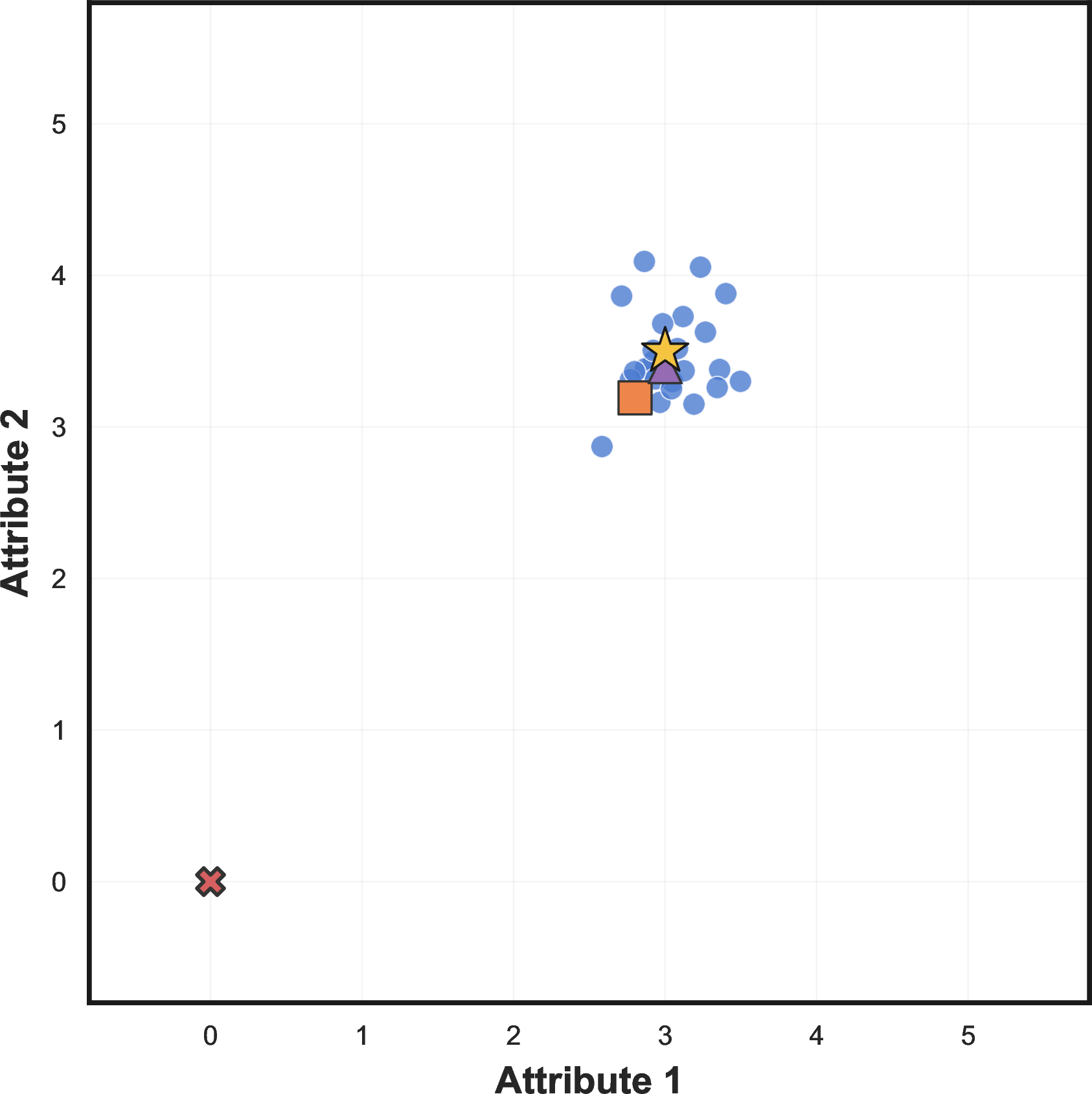
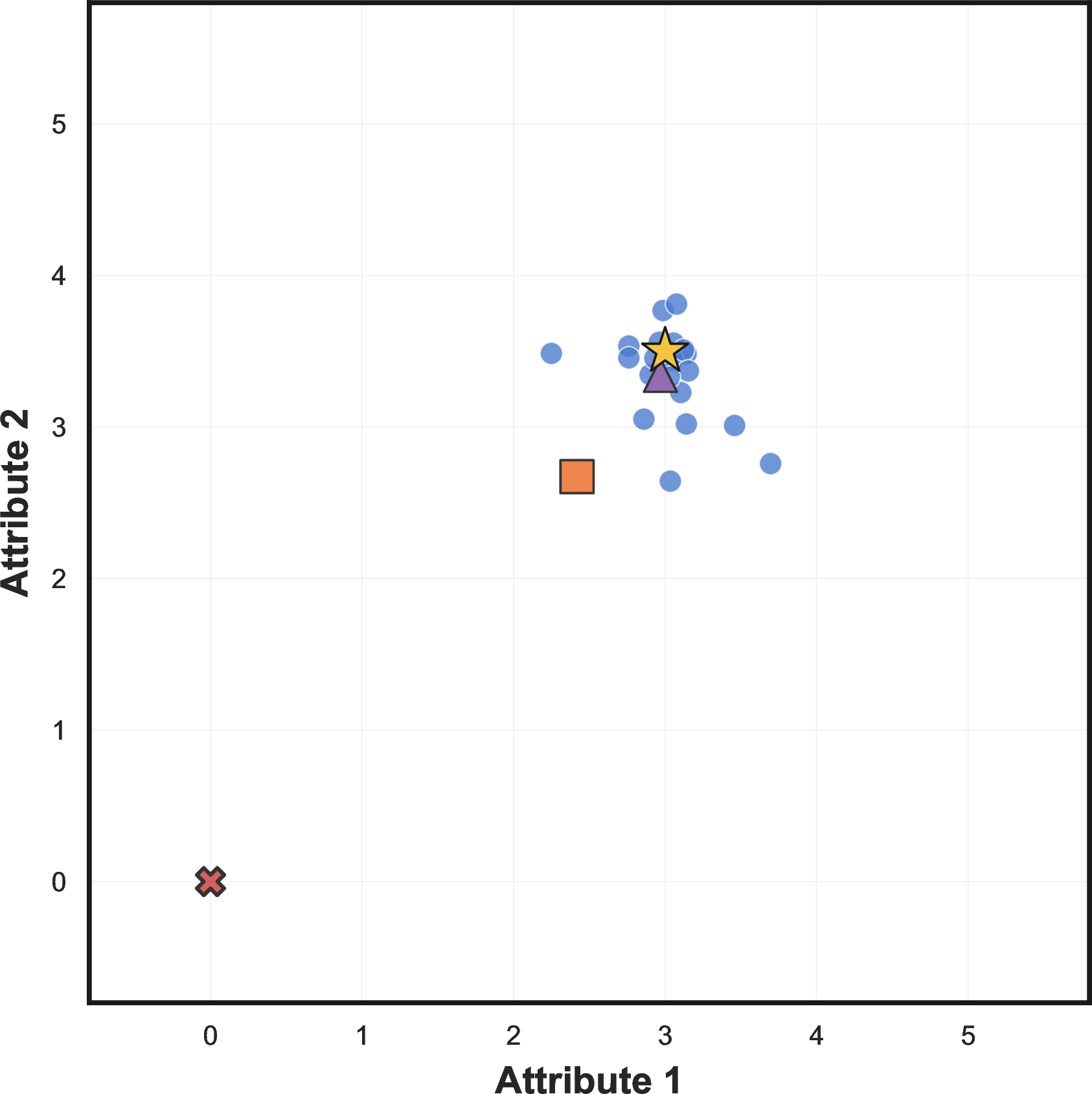
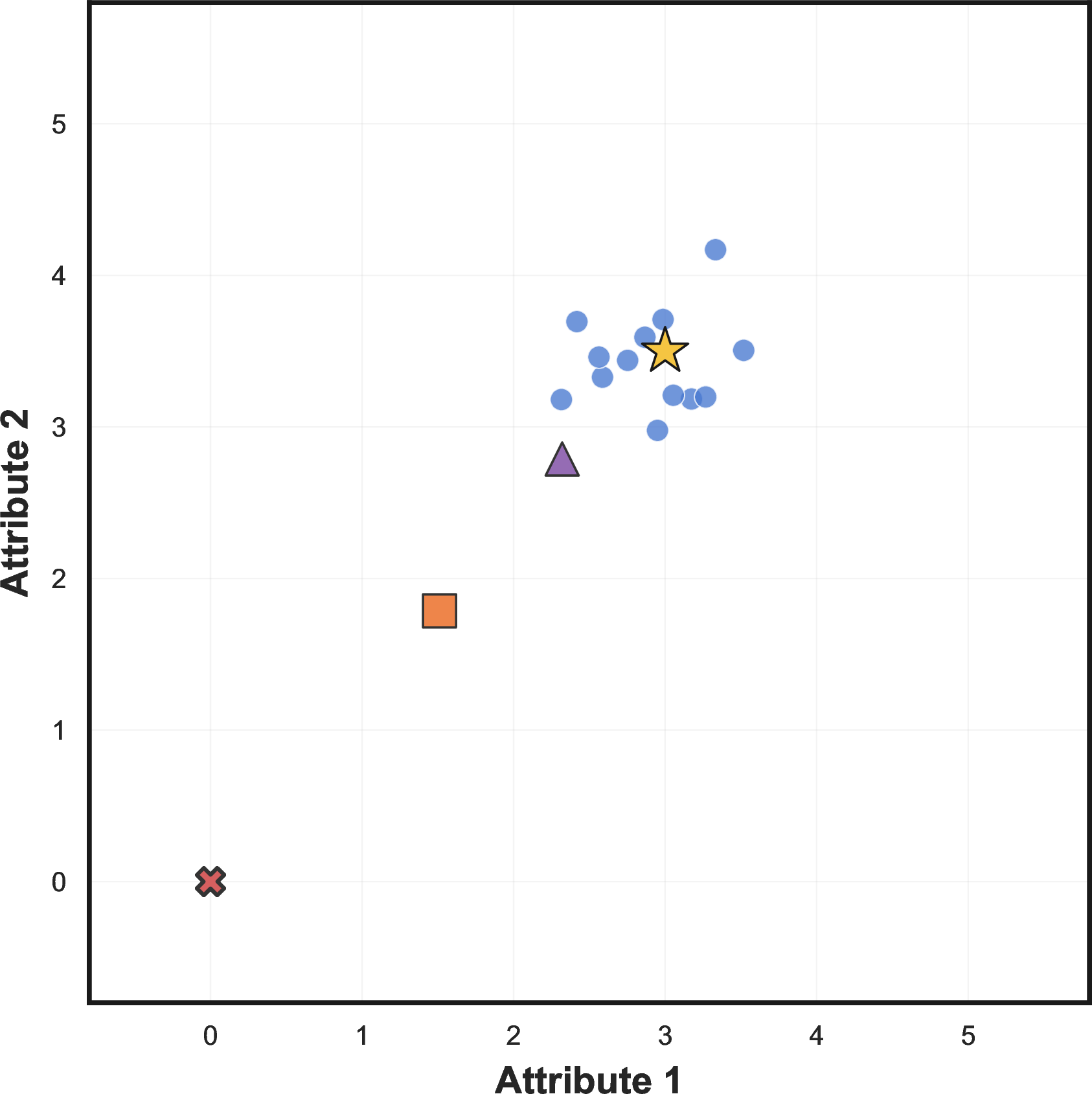
Figure 16: Mode Collapse corruption (\(Q = \delta_{\mathbf{0}}\)). Corrupted judges output the zero vector, modeling parser failures or safety refusals. The mean is pulled linearly toward the origin; at \(\alpha = 0.40\) it lies roughly \(40\%\) of the way from \(\mathbf{y}^\star\) to \(\mathbf{0}\). The geometric median remains within the competent cluster because the majority of Euclidean distances still point toward \(\mathbf{y}^\star\)..
9.1.0.2 Inverted (\(Q = \delta_{K \cdot {\mathbf{1}}- {\mathbf{y}}^{\star}}\)).
The worst-case anti-correlated Byzantine adversary (17). This is the sharpest visual demonstration of the breakdown-point advantage: the corrupted locus and \({\mathbf{y}}^{\star}\) lie on opposite sides of the score space, so at \(\alpha = 0.30\) the mean has already crossed the midpoint while the geometric median remains within the competent cluster.
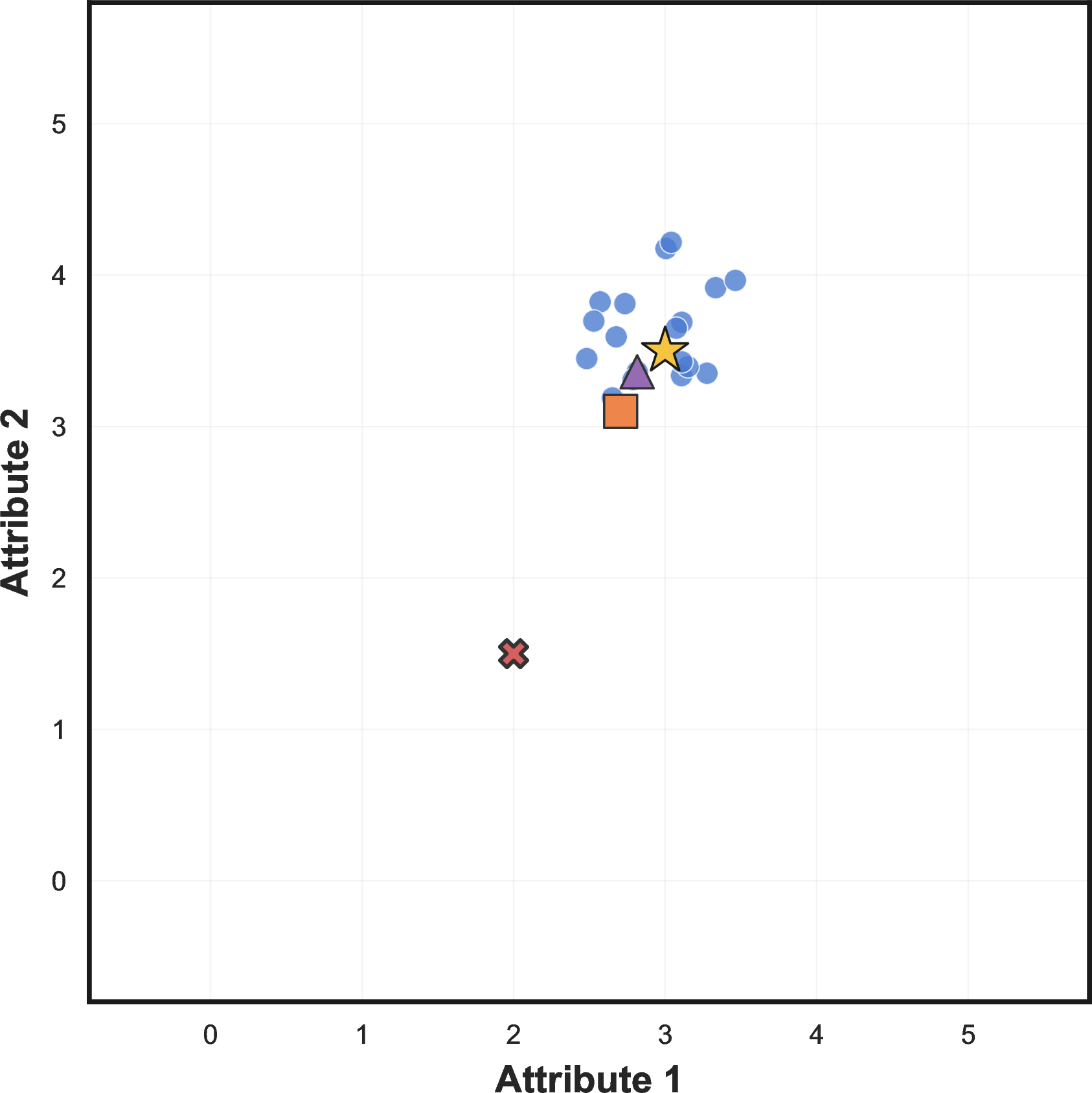
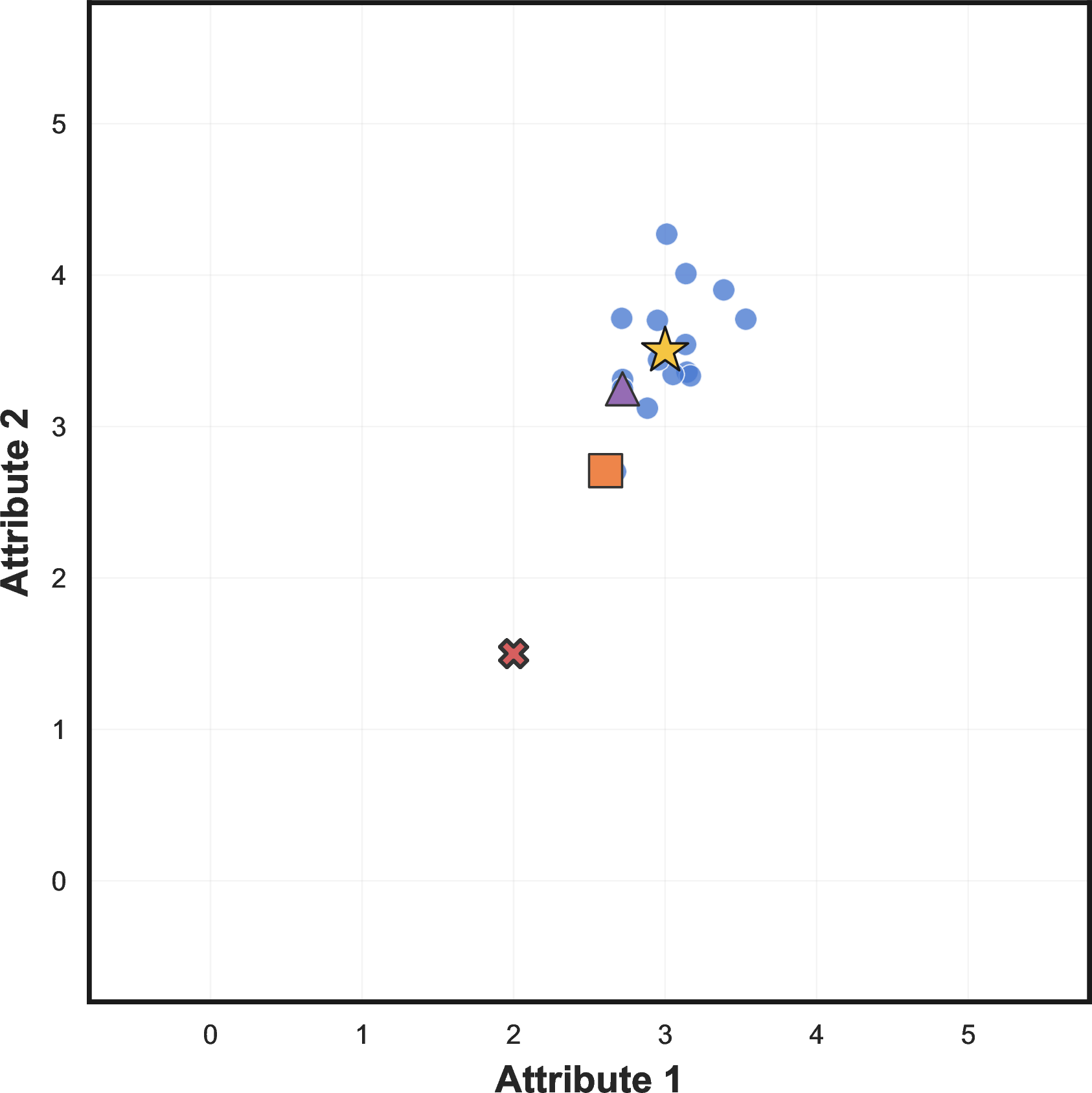
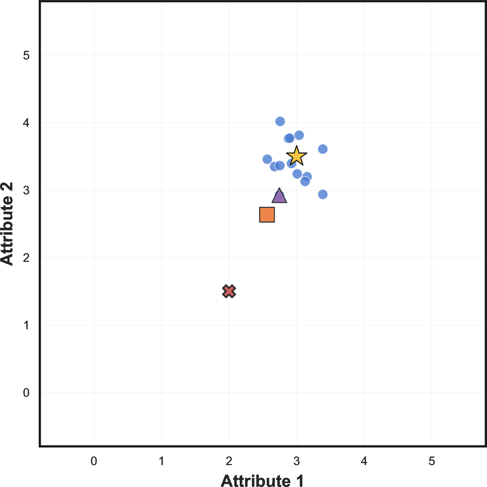
Figure 17: Inverted corruption (\(Q = \delta_{K \cdot \mathbf{1} - \mathbf{y}^\star}\)). The worst-case Byzantine adversary: corrupted scores are perfectly anti-correlated with the truth. The corruption locus and \(\mathbf{y}^\star\) lie on opposite sides of the score space. At \(\alpha = 0.30\) the mean is already displaced past the midpoint, while the geometric median remains close to \(\mathbf{y}^\star\). This is the sharpest demonstration of the breakdown-point advantage..
9.1.0.3 Biased dimension.
Partial competence: correct on one attribute, catastrophically wrong on the other (18). This is the synthetic counterpart of bimodal-random (§6.3) and the
picture of cross-dimensional corruption from Example 1: each corrupted score is plausible per coordinate but jointly anomalous, and the geometric median’s joint-distance
objective resists the off-axis pull that fools per-coordinate alternatives.
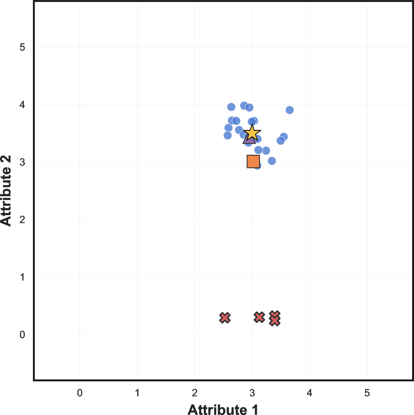
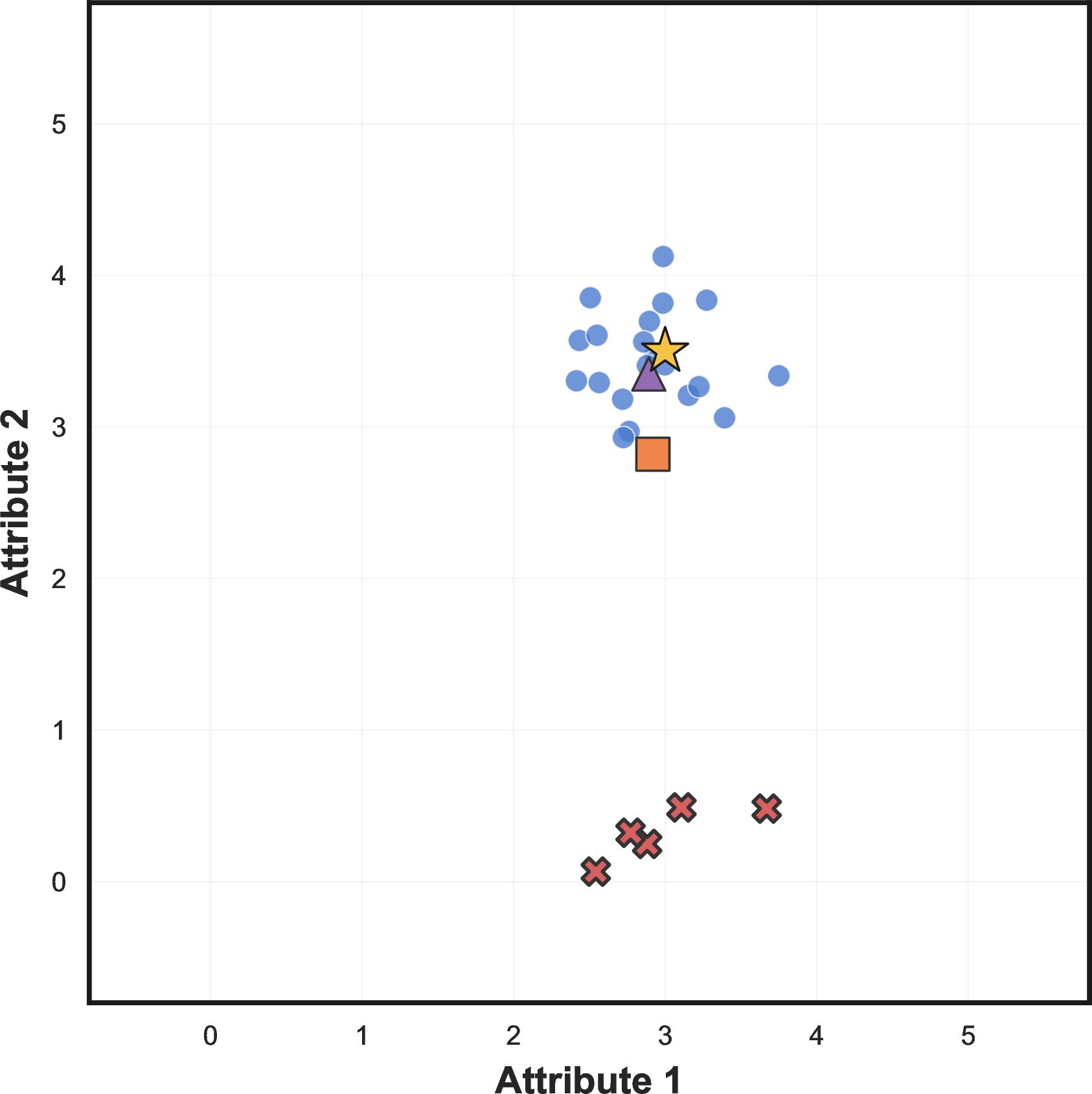
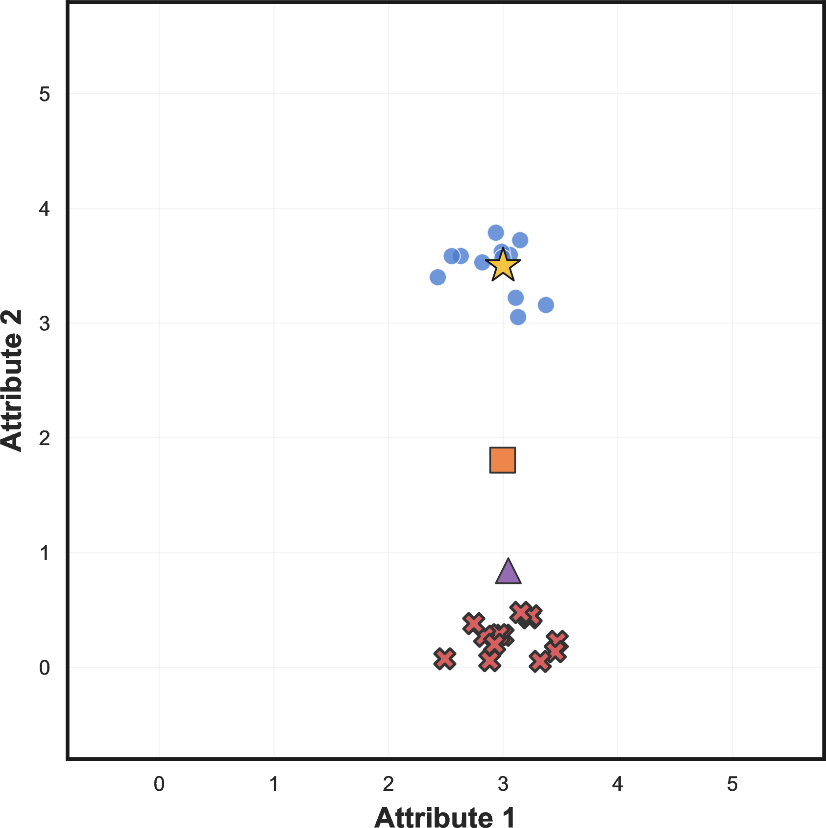
Figure 18: Biased Dimension corruption. Corrupted judges evaluate Attribute 1 correctly but catastrophically fail on Attribute 2 (scores collapse near zero). This partial competence is challenging for coordinate-wise methods because the corruption is invisible on one axis. The geometric median, operating on joint Euclidean distances, detects the anomaly in Attribute 2 and downweights the corrupted points across both dimensions..
9.1.0.4 Random hypercube corners.
The canonical instance of the cross-dimensional class: each corrupted score lands at a vertex of \(\{0, K\}^{d}\) chosen uniformly at random (19). The per-coordinate marginal
\(\frac{1}{2}(\delta_{0}+\delta_{K})\) is indistinguishable from plausible scoring; jointly, every corrupted vector sits at a corner far from \({\mathbf{y}}^{\star}\) in \(\ell_{2}\). This is the “random vertex” generalisation of biased dimension above and exactly the bimodal-random class evaluated empirically in §6.3.


Figure 19: Random hypercube corners (the canonical instance of the cross-dimensional class of Example 1, matching the empirical
bimodal-random class of §6.3). Corrupted judges output an extreme vertex of \(\{0, K\}^{d}\) chosen uniformly at random; per-coordinate the corruption marginal \(\frac{1}{2}(\delta_{0}+\delta_{K})\) is plausible scoring, but the joint vector lies far from \({\mathbf{y}}^{\star}\) in \(\ell_{2}\). The geometric median
resists the cross-dimensional pull (it sits at \({\mathbf{y}}^{\star}\), beneath the gold star), while the arithmetic mean drifts toward the centroid of the corrupted vertices..
9.1.0.5 Sycophantic.
A real-world failure mode in which corrupted judges always rate near the top of the scale—the “everything is great” bias (20). The corrupted cloud sits in the upper-right corner of \([0, K]^{d}\); the arithmetic mean drifts diagonally toward it while the geometric median stays anchored to the competent majority near \({\mathbf{y}}^{\star}\). This complements mode collapse (corruption at the lower-left extremum) at the opposite extreme of the score scale.
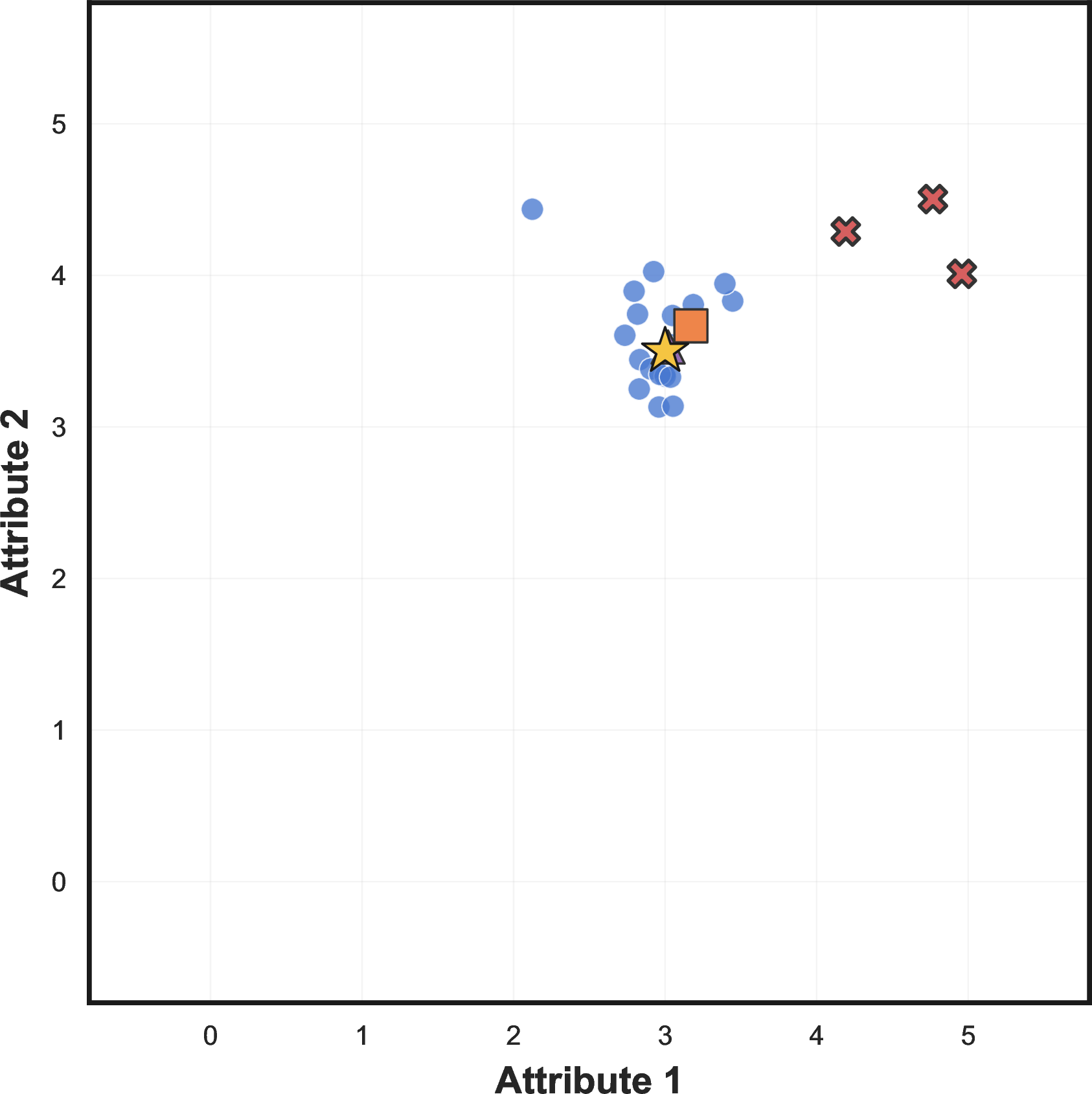
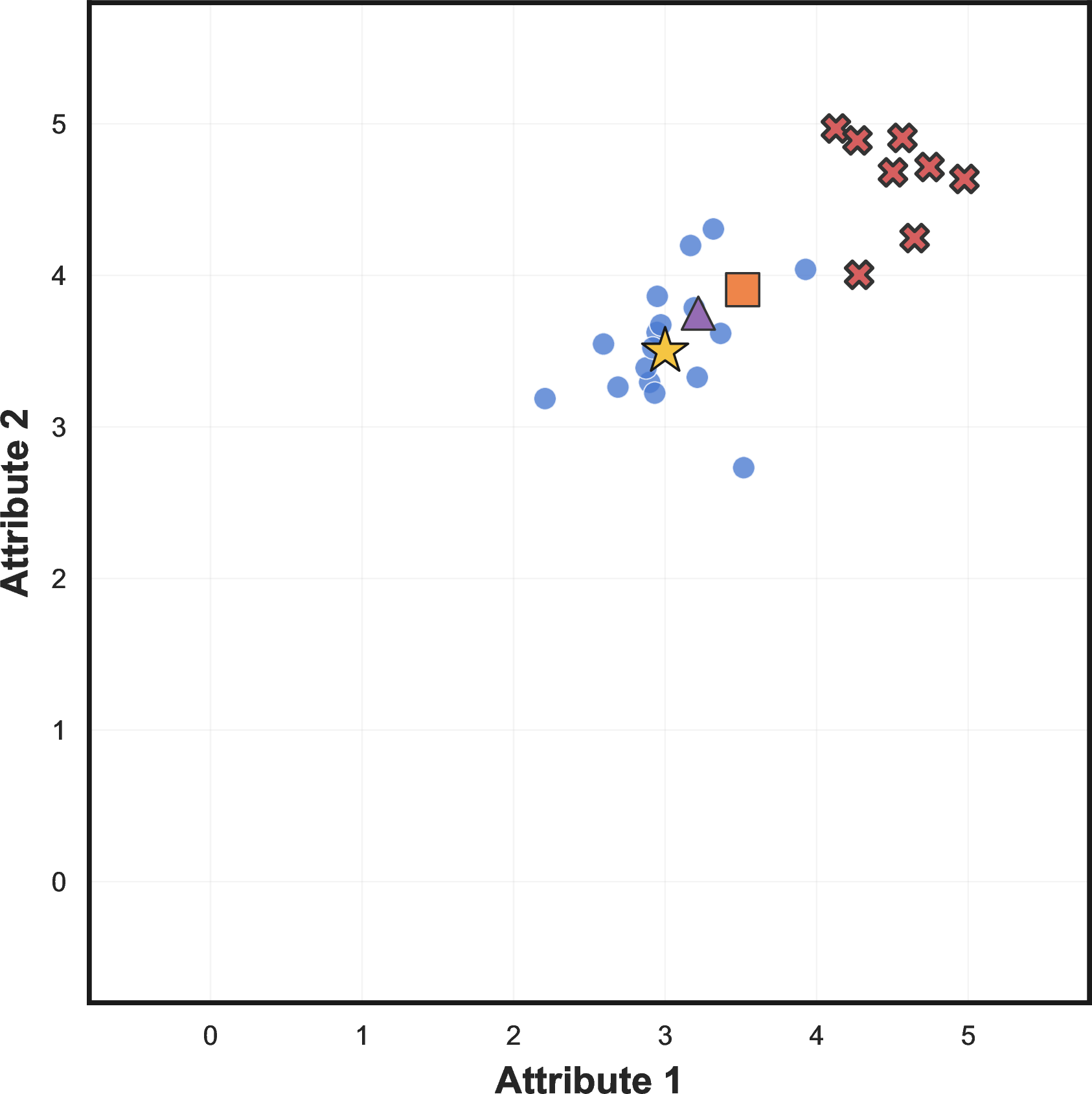
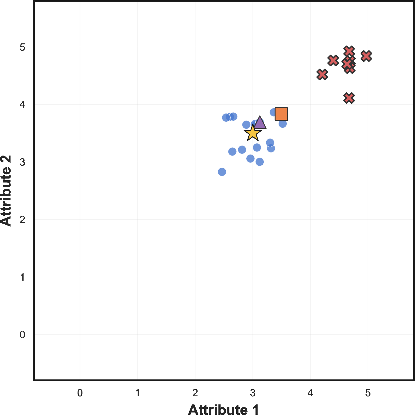
Figure 20: Sycophantic corruption (\(Q = \mathrm{Uniform}([K{-}1, K]^d)\)). Corrupted judges produce scores clustered near the maximum, modeling the “everything is great” failure mode. The corrupted cloud sits in the upper-right corner; the mean drifts diagonally toward it while the geometric median stays anchored to the competent majority near \(\mathbf{y}^\star\)..
9.1.0.6 Summary.
Across all three failure modes, the arithmetic mean acquires a bias proportional to \(\alpha\) and aligned with the corruption locus, while the geometric median remains close to \({\mathbf{y}}^{\star}\) as long as \(\alpha < 1/2\), in agreement with Theorem 1. The complementary Noisy-GT control (§6.7) confirms that this advantage is paid only against biased contamination: when the corruption is benign Gaussian noise, the geometric median does not sacrifice accuracy.
9.2 Per-Model and Per-Dimension Calibration Breakdowns↩︎
The figures in §6 aggregate across rubric dimensions and report the Medium jury’s RMSE. This subsection records the underlying per-model and per-dimension calibration breakdowns on UltraFeedback that motivated the curated three-judge committees of §6.1.
9.2.0.1 Judge set.
The calibration analysis in this subsection includes three closed-API reference judges (Claude Opus, Sonnet, and Haiku 4.5) in addition to the \(13\) open-weight judges of §6.1. The closed-API judges are reference points only — they are not used in any RoPoLL committee — and are included here to contextualise the open-weight calibration patterns.
9.2.0.2 Per-dimension MAE.
21 reports the mean absolute error for each judge against the UltraFeedback rubric dimensions (Helpfulness, Honesty, Instruction Following, Truthfulness). Qwen3 32B and Mistral-Large-3 lead with sub-\(0.75\) MAE across all four dimensions; the Claude family lies near the bottom of the calibration ranking despite strong ranking ability (22 below explains why).

9.2.0.3 Per-dimension mean bias.
22 reports the signed mean bias \(\mathbb{E}[\hat{y}_{i}^{(k)} - y^{\star,(k)}]\) for each (judge, dimension) cell. Two systematic patterns emerge. The Claude family shows uniformly negative bias across all four dimensions (\(-0.5\) to \(-0.8\) on Truthfulness)—a systematic under-scoring tendency. Smaller open-weight models (Magistral Small, Gemma 4B, Nemotron 9B) show uniformly positive bias of comparable magnitude. Qwen3 32B and Qwen3 235B are closest to zero across all dimensions, consistent with their leading MAE. The bias direction is precisely the contamination structure Proposition 2 formalises: mixing systematically over-scoring and under-scoring judges leaves the arithmetic mean’s bias bounded only by the worst per-judge displacement; the geometric median is robust to such mixed-direction biases because the joint subgradient balance does not weight per-coordinate sign.

Corresponding author.↩︎
Dataset released at https://github.com/aws/RoPoLL.↩︎