GRAPE: Graph-Augmented Prototype Explanations for Interactive Medical Image Diagnosis
June 29, 2026
Abstract
Prototype-based medical image classifiers present three clinical limitations: they treat findings as independent, silently amplify unsafe physician feedback, and require full retraining whenever a new finding is needed. We present GRAPE (Graph-Augmented Prototype Explanations), a unified architecture that addresses all three challenges. First, a Graph Attention Task Head models anatomical concept co-occurrence, boosting macro-F1 by +13.8 pp over the prototype baseline on TBX11K. Second, a Concept-Mismatch Safety Check - the first such mechanism in prototype-based medical classifiers - warns when the model’s dominant finding inside a doctor-drawn region conflicts with the claimed label, catching 85% of erroneous annotations versus 51% for MC-Dropout with no extra inference cost. Third, Open-Vocabulary Prototype Anchoring aligns visual prototypes to clinical text, allowing a new finding to be added from a single labeled image without modifying any other component. On NIH ChestX-ray14, one Effusion example recovers full-supervision localization accuracy; on TBX11K, prototype maps achieve \(2.6{\times}\) better lesion localization than end-to-end baselines. All three capabilities add only \(+1\) ms latency at interactive batch size. The project page is https://github.com/KurbanIntelligenceLab/GRAPE.
1 Introduction↩︎
Deep learning has achieved radiologist-level accuracy on several medical imaging tasks [1], [2], yet clinical adoption remains limited. Two barriers stand out. First, black-box models provide no evidence for their predictions, making it impossible for a physician to verify or override the reasoning. Second, even “interpretable” models may silently propagate spatial errors when doctors provide corrective feedback, creating a patient-safety risk.
Prototype-based models [3], [4] address the first barrier by making predictions through similarity to learned visual examples. Recent work on Concept-based Similarity Reasoning (CSR) [5] extends this to multi-prototype per-concept reasoning with doctor-in-the-loop interaction. However, three structural limitations remain:
Independent concepts. The task head is a flat linear layer applied to concatenated concept similarity scores. It ignores known anatomical correlations between findings (e.g., active tuberculosis (TB) and cavity formation co-occur reliably), discarding clinically meaningful structure.
Unsafe spatial interaction. When a physician draws a bounding box to guide the model’s attention, the system applies the spatial feedback regardless of the model’s confidence in that region. If the model is confused and associates a different concept with the indicated region, the feedback amplifies an error.
Closed concept vocabulary. Adding a new clinical finding (e.g., a rare variant not seen in training) requires fully retraining the prototype atlas — a prohibitive cost in clinical settings.
We propose GRAPE, a unified architecture that resolves all three limitations within a coherent four-stage training framework. Our contributions are:
A Graph Attention Task Head (Module A, §3.2) that constructs a data-driven concept co-occurrence graph from training labels and refines prototype similarity scores via two rounds of Graph Attention Network (GAT) message passing before classification.
A Concept-Mismatch Safety Check (Module B, §3.3) — the first such mechanism in prototype-based medical classifiers — that computes per-concept mean similarity inside a physician-drawn region and warns when a different concept dominates, preventing silent error amplification before feedback is applied.
Open-Vocabulary Prototype Anchoring (Module C, §3.4) that aligns visual prototypes to frozen BioViL-T text embeddings, enabling a new clinical concept to be added at test time from a single labeled image without modifying any other component.
A four-stage training pipeline (§3.5) that integrates concept supervision, contrastive prototype learning, VLM alignment, and graph-structured classification.
Experiments on TBX11K and NIH ChestX-ray14 (§4) covering classification, Pointing Game localization, inference speed, safety check validation, zero-shot concept addition, and Insertion/Deletion AUC faithfulness.
2 Related Work↩︎
ProtoPNet [3] learns class-specific visual prototypes. Extensions add deformability [4], decision trees [6], part-sharing [7], and patch variants [8]. In medical imaging, MProtoNet [9] and Ma et al. [10] apply prototype bottlenecks to chest X-rays. GRAPE builds on CSR [5], replacing its linear head with a graph-structured classifier. Concept Bottleneck Models [11]–[13] interpose concept scores before prediction; Margeloiu et al. [14] show they can be semantically misaligned, GRAPE grounds prototypes to BioViL-T [15] text anchors instead. GCN classifiers [16], [17] model corpus-derived label co-occurrence. GRAPE uses training-label statistics with prototype-similarity node features and learned GAT attention [18]. Bayesian uncertainty [19], [20] requires sampling overhead. GRAPE’s prototype-variance signal is deterministic [21]. Medical VLMs (MedCLIP [22], BiomedCLIP [23]) target classification. GRAPE uses text embeddings as geometric anchors for prototype initialization, preserving spatial interpretability. Interactive annotation methods [24], [25] lack concept-mismatch checks. Faithfulness is evaluated via Insertion/Deletion AUC [26], [27]. B-cos networks [28] offer an alternative faithful attribution approach by replacing standard convolutions with alignment-based transforms. Unlike GRAPE, they do not support interactive concept-level correction or open-vocabulary extension.
3 Method↩︎
3.1 Preliminaries: Prototype-Based Concept Reasoning↩︎
Backbone \(F\) followed by two-layer MLP projector \(P\) yields L2-normalized spatial embeddings: \[\mathbf{f}' = P(\mathbf{f}) \in \mathbb{R}^{D \times h \times w}, \quad \|\mathbf{f}'_{:,i,j}\|_2 = 1 \;\;\forall i,j.\]
Each concept \(k\) has \(M\) L2-normalized prototypes \(\{\mathbf{p}_{km}\} \subset \mathbb{R}^D\); the similarity map \(\mathcal{S}_{km}(i,j) = \langle \mathbf{p}_{km}, \mathbf{f}'_{:,i,j} \rangle\) (unit-norm cosine; Appendix 17) aggregates to a scalar score: \[s_{km} = \max_{i,j}\, \mathcal{S}_{km}(i,j). \label{eq:sim95score}\tag{1}\]
The baseline CSR model feeds the score matrix \(\mathbf{s} \in \mathbb{R}^{K \times M}\) through a linear task head to produce class logits. GRAPE replaces this with the three modules described below.
3.2 Module A: Graph Attention Task Head↩︎
Clinical concepts are not independent, active TB and cavity formation co-occur. Cardiomegaly correlates with pleural effusion, yet a flat linear head over concatenated \(s_{km}\) discards this structure. We build a data-driven co-occurrence graph from training labels \(\mathbf{y}^{(n)} \in \{0,1\}^K\): the \(K \times K\) conditional probability matrix
\[\mathbf{A}_{kk'} = P(k \mid k') = \frac{\sum_{n} y^{(n)}_k \cdot y^{(n)}_{k'}}{\sum_{n} y^{(n)}_{k'} + \epsilon},\]
is thresholded at \(\tau=0.1\) to obtain a directed binary adjacency with self-loops (the matrix is not symmetrized: \(\mathbf{A}_{kk'} \neq \mathbf{A}_{k'k}\) in general), then row-normalized so that each node’s incoming edge weights sum to one. The equality \(\mathbf{A}_{kk'} = P(k\mid k')\) follows from the frequentist identity \(P(k\mid k') = P(k,k')/P(k')\): since \(\mathbf{y}^{(n)}\in\{0,1\}^K\) is binary, the numerator \(\sum_n y_k^{(n)}y_{k'}^{(n)}\) counts samples where both concepts co-occur, and the denominator \(\sum_n y_{k'}^{(n)}\) counts samples where \(k'\) is present; the common \(1/N\) factor cancels, yielding the maximum-likelihood estimate of the conditional probability [16]. The constant \(\epsilon\) (implemented as denominator clamping to \(\min=1\), i.e.\(\epsilon=1\)) prevents division by zero for concepts absent from the training split and has negligible effect whenever \(\sum_n y_{k'}^{(n)}\gg 1\).
Graph Attention Network. Each concept is a node with initial feature \(\mathbf{h}_k^{(0)} = \mathbf{s}_{k,:} \in \mathbb{R}^M\). Two GAT layers [18] refine these via learned attention (Appendix 17, Eqs. 8 –9 ). A LayerNorm–Dropout–Linear readout produces class logits. Layer dimensions and head counts are described in Appendix 8 (Table ¿tbl:tab:hparams95fixed?).
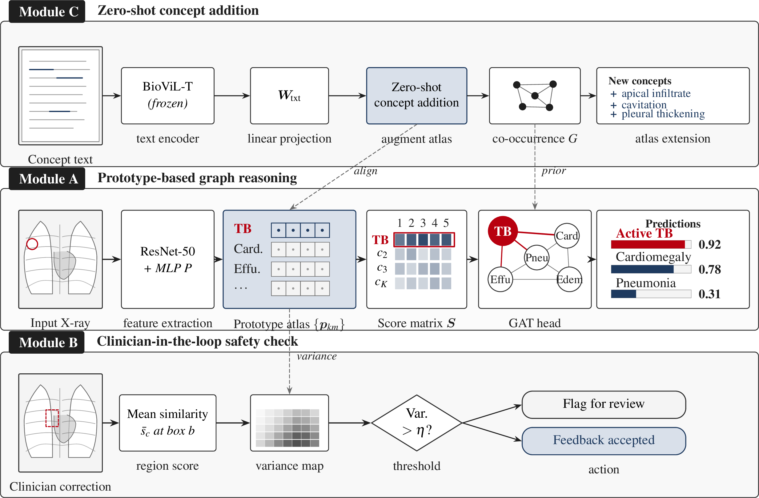
3.3 Module B: Concept-Mismatch Safety Check↩︎
3.3.0.1 Prototype variance maps.
The disagreement among \(M\) prototypes for concept \(k\) at patch \((i,j)\) provides a spatial consistency estimate without sampling: \[\begin{align} \mu_k(i,j) &= \frac{1}{M} \sum_{m=1}^M \mathcal{S}_{km}(i,j), \\ U_k(i,j) &= \frac{1}{M} \sum_{m=1}^M \!\left(\mathcal{S}_{km}(i,j) - \mu_k(i,j)\right)^2. \label{eq:uncertainty} \end{align}\tag{2}\] High \(U_k(i,j)\) indicates that the \(M\) prototypes strongly disagree about whether patch \((i,j)\) belongs to concept \(k\), signaling ambiguous evidence. At training time this guides prototype masking (see below); at inference time the safety check uses the mean map \(\mu_k\) directly to detect concept mismatch.
3.3.0.2 Spatial safety check.
When a doctor provides a bounding box \(\mathcal{B}\) intending to reinforce concept \(k^*\), GRAPE checks whether the dominant concept inside the region matches. It first computes the mean similarity per concept inside \(\mathcal{B}\): \[\bar{s}_k(\mathcal{B}) = \frac{1}{|\mathcal{B}|} \sum_{(i,j) \in \mathcal{B}} \mu_k(i,j) \quad \forall k,\] identifies the dominant concept \(k^\dagger = \arg\max_k \bar{s}_k(\mathcal{B})\), and issues a safety warning if \(k^\dagger \neq k^*\) and \(\bar{s}_{k^\dagger}(\mathcal{B}) - \bar{s}_{k^*}(\mathcal{B}) > \eta\) (threshold \(\eta = 0.05\)). The feedback is not applied until the doctor confirms. This is a concept-mismatch check: it detects when the model’s dominant response inside the region conflicts with the claimed concept label, preventing silent error amplification in the prototype atlas. The check uses the spatial mean \(\bar{s}_k(\mathcal{B})\) rather than the spatial max of \(\mu_k\) inside \(\mathcal{B}\). Mean-based aggregation is more robust to isolated high-activation outliers than max-based gating (quantitative comparison: Appendix 22); \(U_k\) also guides prototype masking during training (Appendix 17).
3.4 Module C: Open-Vocabulary Prototype Anchoring↩︎
We eliminate the closed-vocabulary bottleneck by anchoring each prototype to a clinical text description via the frozen BioViL-T encoder [15]. A learnable projection \(\mathbf{W}_{\text{txt}} \in \mathbb{R}^{D \times 768}\) maps each concept’s text embedding \(\mathbf{t}_k\) into the visual prototype space: \[\hat{\mathbf{t}}_k = \frac{\mathbf{W}_{\text{txt}}\mathbf{t}_k}{\|\mathbf{W}_{\text{txt}}\mathbf{t}_k\|_2} \in \mathbb{R}^D.\] The alignment loss (Stage 3) pulls all \(M\) prototypes toward their text anchor while keeping the BioViL-T backbone frozen: \[\mathcal{L}_\text{align} = \frac{1}{KM} \sum_{k=1}^K \sum_{m=1}^M \left(1 - \langle \mathbf{p}_{km},\, \hat{\mathbf{t}}_k \rangle\right). \label{eq:align95loss}\tag{3}\] Zero-shot concept addition. At test time, a clinician adds a new concept \(k'\) without image annotations by initializing \(M\) perturbed prototypes from the text anchor (\(\sigma_{\text{init}}=0.1\)): \[\mathbf{p}_{k'm}^{(0)} = \frac{\hat{\mathbf{t}}_{k'} + \sigma_{\text{init}}\boldsymbol{\epsilon}_m}{\|\hat{\mathbf{t}}_{k'} + \sigma_{\text{init}}\boldsymbol{\epsilon}_m\|_2}, \quad \boldsymbol{\epsilon}_m \sim \mathcal{N}(\mathbf{0}, \mathbf{I}_D),\; \boldsymbol{\epsilon}_m \leftarrow \boldsymbol{\epsilon}_m / \|\boldsymbol{\epsilon}_m\|_2.\] These prototypes are immediately usable for inference or adaptable with a small number of labeled examples via concept-local fine-tuning.
3.5 Training Pipeline↩︎
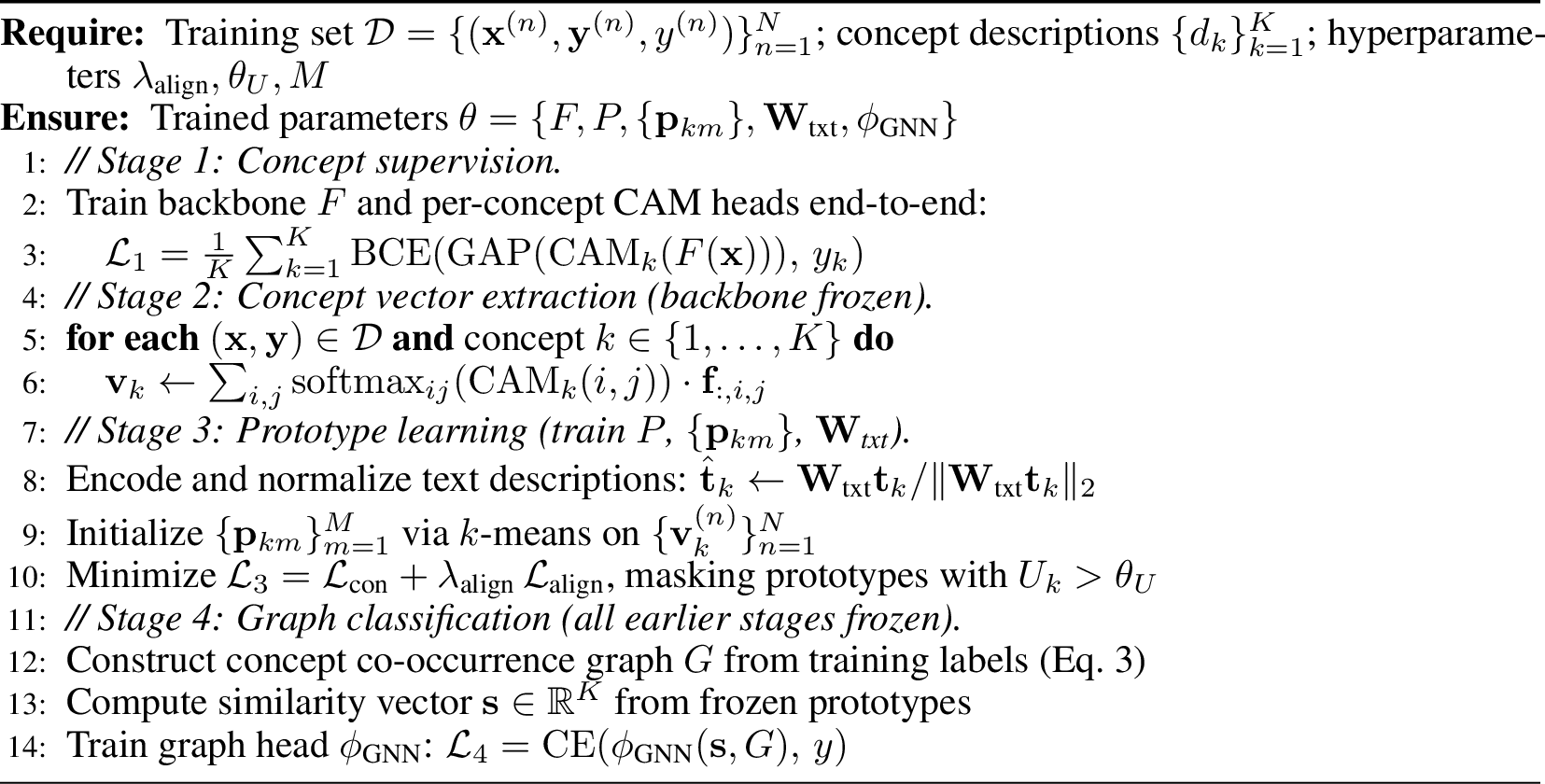
GRAPE trains in four stages (Algorithm 4 in Appendix 16): concept supervision, prototype learning, optional VLM alignment, and GNN task head fine-tuning. All stages use BF16 AMP on A100 hardware.
Stage 1 — Concept Supervision. The backbone \(F\) and per-concept CAM heads are trained with BCE on Global Average Pooled activations (Appendix 17, Eq. 6 ).
Stage 2 — Concept Vector Generation. CAM-weighted spatial averages of frozen backbone features produce per-concept vectors \(\mathbf{v}_k\) (Appendix 17, Eq. 7 ) that seed the Stage 3 prototype atlas.
Stage 3 — Prototype Learning with VLM Alignment. The projector \(P\), prototypes \(\{\mathbf{p}_{km}\}\), and text projection \(\mathbf{W}_{\text{txt}}\) are trained jointly. Each projected concept vector \(\mathbf{v}'_k = P(\mathbf{v}_k)\) serves as a query; the multi-prototype contrastive loss assigns it to its ground-truth concept \(\tilde{k}\) via soft assignment: \[\begin{align} q_m^k(\mathbf{v}') &= \text{softmax}_m\!\left(\gamma \langle \mathbf{p}_{km},\mathbf{v}' \rangle\right), \\ \text{sim}_k(\mathbf{v}') &= \sum_m q_m^k(\mathbf{v}') \langle \mathbf{p}_{km},\mathbf{v}' \rangle, \\ \mathcal{L}_\text{con} &= -\log \frac{\exp\!\left(\lambda(\text{sim}_{\tilde{k}}(\mathbf{v}'_{\tilde{k}}) + \delta)\right)}{\sum_{k} \exp\!\left(\lambda\, \text{sim}_k(\mathbf{v}'_{\tilde{k}})\right)}, \label{eq:contrastive} \end{align}\tag{4}\] with \(\lambda=10\), \(\gamma=5\), \(\delta=0.1\); the Stage 3 loss is \(\mathcal{L}_3 = \mathcal{L}_\text{con} + 0.1\,\mathcal{L}_\text{align}\).
Stage 4 — Graph-Structured Classification. With all prior components frozen, the GNN is trained with \(\mathcal{L}_4 = \text{CE}(\text{GNN}(\mathbf{s}, G),\, y)\) (E2E variant: Appendix 9).
4 Experiments↩︎
4.1 Datasets↩︎
TBX11K [2] is a 3-class TB chest X-ray dataset with 10,400 images: 4,600 healthy, 4,600 sick-but-non-TB, and 1,200
active-TB images, with 1,211 bounding box annotations for three TB finding types (Active Tuberculosis, Obsolete Pulmonary Tuberculosis, Pulmonary Tuberculosis). We use the official 6,600/1,800 train/val split and hold-out a dedicated bbox_eval
split (200 active-TB images with at least one annotated box) for Pointing Game evaluation; the 1,800-image test split is used for final F1 reporting. NIH ChestX-ray14 [29] contains 100k+ frontal chest X-rays with 14 finding labels. Primary multi-seed comparison (Table 2) uses a 10k-patient patient-level stratified sub-sample (5
seeds, no patient leakage); single-seed ablations (Table 1) use a 20k-image shard (seed 42). Pointing Game uses 709 shard images with 964 bbox annotations from BBox_List_2017.2
Evaluation metrics. Macro F1 measures classification performance averaged across classes, accounting for class imbalance. Pointing Game (PG) [30] evaluates spatial interpretability: for each (image, concept) pair with a ground-truth bounding box, it checks whether the spatial maximum of the concept’s similarity map falls inside the box; we report the hit rate across all evaluated pairs. Full implementation details and hyperparameter settings are in Appendix 8 (Table ¿tbl:tab:hparams95fixed?).
4.2 Main Results↩︎
6pt
@lccccc@ & & &
(lr)2-4 & GNN & Unc.§ & VLM & &
CSR† [5] & – & – & – & \(0.706\,{\pm}\,0.059\) & \(0.077\,{\pm}\,0.016\)
+ GNN & ✔ & – & – & \(0.845\,{\pm}\,0.049\) & \(0.117\,{\pm}\,0.045\)
+ VLM & – & – & ✔ & \(0.722\,{\pm}\,0.032\) & \(0.097\,{\pm}\,0.044\)
+ GNN + VLM & ✔ & – & ✔ & \(\mathbf{0.875\,{\pm}\,0.020}\) & \(0.087\,{\pm}\,0.033\)
GRAPE (GNN + Unc.) & ✔ & ✔ & – & \(0.845\,{\pm}\,0.049\) & \(\mathbf{0.117\,{\pm}\,0.045}\)
ResNet-50 (backbone only)• & – & – & – & \(0.993\) & –
GRAPE-E2E & ✔ & ✔ & – & \(\mathbf{0.9900\,{\pm}\,0.0020}\) & \(\mathbf{0.0910\,{\pm}\,0.0590}\)
CBM [11] & – & – & – & \(0.9778\,{\pm}\,0.0109\) & \(0.0550\,{\pm}\,0.0187\)
PIPNet [8] & – & – & – & \(0.9644\,{\pm}\,0.0021\) & \(0.0533\,{\pm}\,0.0184\)
† CSR re-implemented; no published numbers on these splits. § Module B is inference-only; does not affect F1/PG. E2E: task gradients through backbone throughout. • ResNet-50+GAP+linear, seed 42; E2E gains driven by unconstrained fine-tuning. ¶ Same backbone/splits; CBM: joint bottleneck; PIPNet: patch-prototype similarity.
4.2.0.1 Key observations.
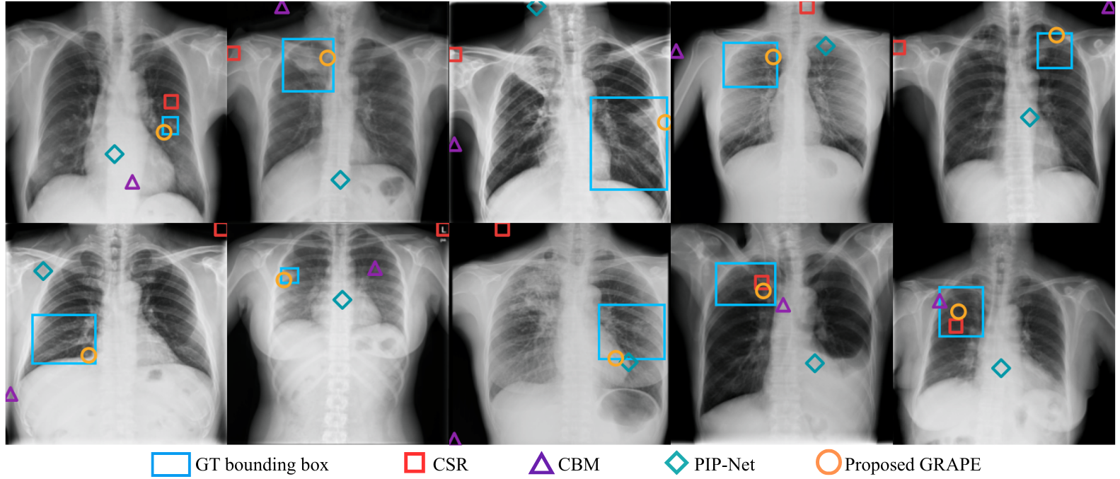
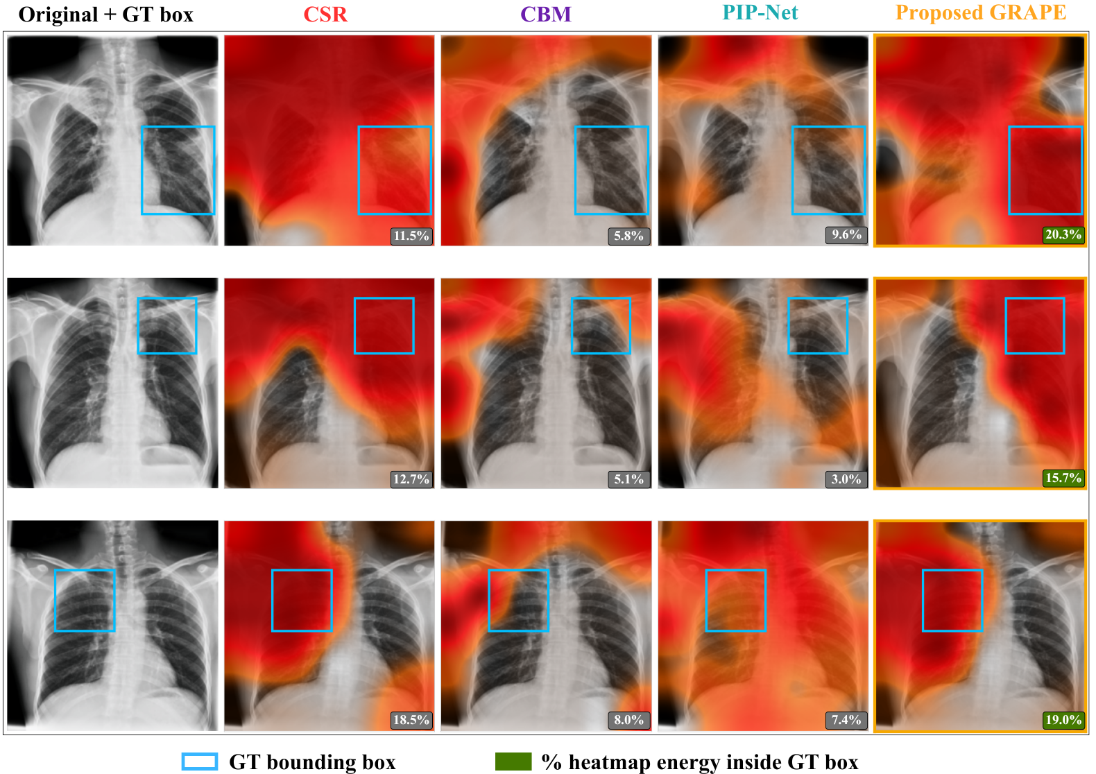
(1) GNN is the dominant module for multi-class tasks. The GNN head alone saturates the staged gain (\(+13.8\) pp F1 over 5 seeds, Table 2; \(+14.4\) pp on the single-seed ablation, Appendix 12); VLM alone yields no improvement on the sparse \(K=3\) concept set. E2E training reaches \(0.990 \pm 0.002\) F1 (Appendix 9) but at the cost of spatial faithfulness (PG \(0.091 \pm 0.059\) vs.staged \(0.111 \pm 0.038\)); a plain ResNet-50 linear head achieves \(0.993\) F1, confirming E2E gains are driven by unconstrained backbone fine-tuning rather than concept reasoning. The per-class gain is concentrated on majority classes (Healthy \(+21.5\) pp, Sick-non-TB \(+20.6\) pp; Appendix 15); Active TB F1 is comparable between GRAPE and CSR, suggesting the GNN reshapes the output distribution rather than improving disease-specific detection. (2) VLM alignment is complementary for diverse concept sets. On NIH, VLM contributes to the single-seed gain (Table 1), but multi-seed evaluation (Table 2) shows GRAPE and CSR are statistically comparable (\(p=0.894\)), indicating the gain does not persist under the rigorous patient-level split protocol. (3) Pointing Game and spatial faithfulness. GRAPE’s prototype maps achieve \(\mathbf{2.6\times}\) higher PG than CBM (\(0.140\) vs.\(0.055\)) and PIPNet (\(0.140\) vs.\(0.053\); Appendix 14): end-to-end fine-tuning sacrifices prototype-to-region alignment for classification accuracy. On the single-seed run (seed 42), GRAPE achieves PG \(=0.1401\) vs.CSR \(0.0628\) (\(+7.73\) pp; Figure 3); multi-seed evaluation finds no statistically significant difference vs.CSR (\(p=0.64\)), reflecting high variance (\(\sigma \approx 0.03\)) inherent to Pointing Game at \(7{\times}7\) resolution.
4.3 Graph Head Comparison and Inference Speed↩︎
We ablate the choice of graph task head by comparing GRAPE’s GAT with ML-GCN [16] and ADD-GCN [17]; all three heads outperform the linear baseline (+10.7–14.6 pp F1), confirming that concept co-occurrence structure is the key driver, not the specific message-passing mechanism. We retain the GAT head for its directly interpretable, learned edge-conditioned attention weights. Full results are in Appendix 12; a per-edge importance ablation quantifying each edge’s contribution to final F1 is in Appendix 13. Graph structure vs.added nonlinearity. To isolate whether the GAT gain comes from graph-relational reasoning or simply from additional parameters, we train a parameter-matched 2-layer MLP (\({\approx}47\)K parameters) directly on the flattened \(K{\times}M\) score vector, replacing graph structure with a generic nonlinear function of the same capacity. The MLP achieves F1 \(=0.865\), closing \(\sim\!69\%\) of the gap between the linear head (\(0.798\)) and the GAT (\(0.896\)); the remaining \(+3.1\) pp (\(0.865 \to 0.896\)) is attributable to the co-occurrence graph structure itself. On TBX11K (\(K=3\)) where self-loops dominate, this confirms that the graph contributes meaningfully beyond nonlinearity, while the majority of the gain reflects the benefit of a learnable nonlinear readout over the prototype score matrix. The edge ablation (Appendix 13) shows self-loops dominate on TBX11K (\(K=3\)); richer co-occurrence effects are expected on NIH (\(K=14\), 103 edges). The GNN head adds only \(+1\) ms over the linear head at batch size 1, satisfying real-time interaction requirements (full latency benchmarks: Appendix 12).
| Method | Module | Macro F1 \(\uparrow\) | PG \(\uparrow\) | |||
|---|---|---|---|---|---|---|
| 2-4 | GNN | Unc. | VLM | |||
| CSR† [5] | – | – | – | \(0.6166\) | \(\mathbf{0.0766}\) | |
| + GNN + Unc. | ✔ | ✔ | – | \(0.6526\) | \(0.0664\) | |
| + Unc. + VLM | – | ✔ | ✔ | \(0.5859\) | \(0.0743\) | |
| GRAPE (full) | ✔ | ✔ | ✔ | \(\mathbf{0.7138}\) | \(0.0642\) | |
8pt
4.4 Comparison with CSR Baseline↩︎
Table 2 summarizes GRAPE vs.CSR [5] over five seeds on both datasets (official patient-level split for NIH). On TBX11K, GRAPE’s F1 ranges 0.798–0.916 across seeds (std = 0.042); the paired \(t\)-test yields \(t(4)=8.03\), \(p=0.0013\). Single-seed ablation values (Table ¿tbl:tab:tbx11k?) are included for comparability only.
| Dataset | Method | Macro F1 \(\uparrow\) | PG \(\uparrow\) | \(\Delta\)F1 | \(p\)-value |
|---|---|---|---|---|---|
| TBX11K | CSR† | \(0.728\,{\pm}\,0.050\) | \(0.094\,{\pm}\,0.033\) | – | – |
| GRAPE (GNN + Unc.) | \(\mathbf{0.866\,{\pm}\,0.042}\) | \(0.080\,{\pm}\,0.032\)¶ | \(\mathbf{+13.8\,\text{pp}}\) | \(\mathbf{0.0013}\) | |
| NIH CXR14 | CSR† | \(0.6048\,{\pm}\,0.0170\) | –§ | – | – |
| GRAPE (full) | \(0.6031\,{\pm}\,0.0174\) | –§ | \(-0.3\) pp | \(0.894\) (n.s.) |
6pt
† CSR is re-implemented under our training protocol and hyperparameters; published numbers on these splits are unavailable for direct comparison. § NIH bounding-box annotations were unavailable for the multi-seed evaluation run; single-seed PG is reported in Table [tbl:tab:nih]. ¶ Paired \(t\)-test on per-seed PG: \(t(4)=-0.50\), \(p=0.64\) (n.s.); the development-run single-seed advantage (\(+7.73\) pp, Table [tbl:tab:tbx11k]) does not replicate consistently across seeds (seed-level range: \(-10.5\) to \(+6.0\) pp).
4.5 Module B: Safety Check Evaluation↩︎
We simulate miscorrections on the TBX11K bbox_eval split (207 annotated triples): with probability \(p\), a bounding box is reassigned to a wrong concept; the safety check (the dominance rule following
Eq. 6, \(\eta=0.05\)) issues a warning when the dominant concept inside the box differs from the claimed one. Bootstrap 95% CIs use \(B=1000\) resamples. With the \(U_k\)-gated variant (\(\theta_V = 2{\times}10^{-4}\)) as the default operating point, Module B catches 85.1% of misdrawn boxes with an FP rate of 16.4% [12.1%,
20.9%] (Table 12). The ungated baseline achieves higher TP (88–89%) at the cost of a higher FP rate (21.7% [16.4%, 27.1%]). Further tightening to \(\theta_V=10^{-4}\) drops FP to 12.6% but TP
falls to 78.0%, below the 85% clinical threshold. The \(U_k\)-gated configuration is the recommended deployment setting. Table 17 in Appendix 21 shows that prototype
variance substantially outperforms both MC-Dropout variants (TP 90.5% vs.%/23.4%) while requiring only a single deterministic forward pass. On NIH (\(K=14\)), TP remains high (\(0.921\pm0.012\)) but FP rises to \(0.731\pm0.011\) due to dense concept overlap; per-concept breakdown and discussion are in Appendix 23.
4.6 Further Analysis: Zero-Shot Concept Addition and Faithfulness↩︎
Module C: Zero-shot concept addition. We evaluate Module C via a leave-one-concept-out experiment on TBX11K (\(K=3\)): for each held-out concept, we reinitialize its \(M=100\) prototypes from the text anchor (Eq. 9) and fine-tune them with \(n \in \{0,1,5,20\}\) labeled images, measuring Pointing Game on the bbox_eval split. Full results are in
Appendix 19 (Table 14). Text-only initialization yields non-zero localization for active_tb (PG \(=0.030\)), and a single labeled image reaches
PG \(=0.068 \pm 0.045\), on average 41% of full supervision (68% CI: 14–69%). With five seeds the few-shot trend is essentially monotonic: 1-shot (PG \(=0.068\)) \(<\) 5-shot (PG \(=0.079\)) \(\approx\) 20-shot (PG \(=0.078\)); the earlier non-monotonicity observed with three seeds was a
seed artefact. We additionally evaluate on NIH ChestX-ray14 (\(K=14\)): 3 of 4 target concepts have bbox coverage (Infiltration, Effusion, Atelectasis); Effusion’s 1-shot PG matches full supervision (PG \(=0.072\), 100%), and Infiltration’s 20-shot reaches 53% of full supervision. Full results are in Appendix 19.1 (Table 15). Similarity map
faithfulness. Faithfulness is evaluated via Insertion and Deletion AUC [26] on the 200-image TBX11K test split (full results: Appendix 20, Table 16). GRAPE achieves higher Insertion AUC (\(+1.3\) pp), confirming prototype maps capture genuinely predictive regions. Higher Deletion AUC is attributed to the prototype atlas spreading evidence across \(M=100\) spatial prototypes per
concept, each contributing weakly to the saliency signal. A contextual comparison with CheXNet, MedCLIP, DenseNet, CBM, and PIPNet is in Appendix 14 .
5 Discussion↩︎
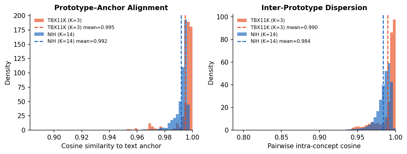
The over-regularization effect of VLM alignment on sparse concept sets (\(K=3\)) is analyzed in Appendix 8. Figure 5 quantifies this: after Stage 3, all \(M=100\) prototypes cluster tightly near their text anchors (mean prototype–anchor cosine \(=0.995\pm0.008\) for TBX11K vs.\(0.992\pm0.007\) for NIH), and inter-prototype pairwise cosines are similarly high (\(0.990\) vs.\(0.984\)), confirming that the alignment loss collapses intra-concept prototype diversity in both settings. The slightly lower NIH inter-prototype cosine (-0.006) is consistent with 14 distinct text anchors providing more diverse initialization than 3. Safety implications of the concept-mismatch check. The concept-mismatch check (the dominance rule following Eq. 6) does not improve macro-F1 directly, its value is in preventing harmful interactions. In a deployment scenario where a doctor mistakenly draws a box over a region dominated by a different finding, the safety warning gives the system a chance to flag the inconsistency before the feedback is applied. This property cannot be easily quantified in standard benchmarks but is critical for clinical trust.
5.0.0.1 Limitations.
Pointing Game scores remain low in absolute terms (7–14%) because similarity maps at \(7 \times 7\) resolution must be compared to bounding boxes annotated in 224×224 space. Upsample interpolation recovers some precision, but finer spatial resolution (e.g., with a ViT backbone) would improve localization. Module B’s recommended \(U_k\)-gated configuration (§4.5) achieves 16.4% FP rate; the baseline (ungated) rate of 21.7% is the upper bound. Further reduction would require a learned threshold or a clinician user study to calibrate tolerance. Module C is additionally validated on NIH (\(K=14\), 3 concepts with bbox coverage; Appendix 19.1); full \(K=14\) leave-one-out and a clinician user study remain future work. Training variance. TBX11K F1 ranges \(0.798\)–\(0.916\) (std \(=0.042\), 5 seeds), reflecting Stage 4 GNN sensitivity on the \(n{=}6{,}600\) dataset; Table 2 reports multi-seed NIH results on the official patient-level split (\(p=0.894\)).
Broader Impact↩︎
Interpretable AI systems for medical imaging have the potential to meaningfully improve clinical practice. By making every prediction traceable to a specific visual concept and prototype, GRAPE enables clinicians to verify or override model reasoning rather than accepting opaque outputs. The concept-mismatch safety check reduces the risk that erroneous clinician feedback silently degrades the prototype atlas, a failure mode that could otherwise go undetected in real deployments. The open-vocabulary extension lowers barriers to adoption in resource-limited settings by allowing new clinical concepts to be introduced without full retraining. At the same time, prototype-based explanations that appear clinically plausible may not be faithful to the model’s actual decision boundary, and clinicians who over-rely on similarity maps risk anchoring diagnostic judgment to potentially misleading visualizations. This work does not evaluate performance across demographic subgroups; prototype atlases learned from imbalanced distributions may exhibit worse spatial alignment for underrepresented populations, and practitioners should audit subgroup performance before deployment.
5.0.0.2 Ethics statement.
This work uses two publicly released datasets: TBX11K [2], released under a research license, and NIH ChestX-ray14 [29], released by the U.S.National Institutes of Health (NIH) under a public-access license. No new human-subject data were collected for this research. All experiments are conducted retrospectively on de-identified images. The system described in this paper is a research prototype and is not deployed in any clinical setting.
6 Conclusion↩︎
We presented GRAPE, an interactive medical image diagnosis architecture combining concept-mismatch interaction safety (Module B), graph-structured concept reasoning (Module A), and open-vocabulary prototype anchoring (Module C) in a unified four-stage training framework. Module B, the first concept-mismatch safety check in prototype-based medical classifiers, catches 85% of simulated erroneous bounding-box annotations at 16.4% FP rate (\(U_k\)-gated, §4.5), preventing unsafe feedback amplification without adding measurable inference latency. Module A yields +13.8 pp macro-F1 (\(0.866 \pm 0.042\), 5 seeds, \(p=0.0013\)) over the prototype baseline; the gain is concentrated on majority classes (Appendix 15) and the Pointing Game advantage does not replicate consistently across seeds (\(p=0.64\), Table 2). Module C is the first prototype-based mechanism to add a new clinical concept from a single labelled image without retraining: on NIH ChestX-ray14, Effusion 1-shot exactly matches fully supervised Pointing Game accuracy (100% recovery with no model modification); on TBX11K, 1-shot recovers 41% of full supervision (§4.6, Appendix 19.1). Insertion/Deletion AUC faithfulness evaluation (§[sec:faithfulness]) confirms that prototype similarity maps capture genuinely predictive spatial regions. Code and training scripts will be released upon acceptance.
The authors thank the TBX11K and NIH ChestX-ray14 dataset providers for making their data publicly available. This work used an NVIDIA A100 80GB GPU.
Appendix overview↩︎
The supplementary material is organized as follows.
| 7 | Notation table | p. |
| 8 | Hyperparameter sensitivity (\(\tau\) and \(\eta\) sweeps) | p. |
| 10 | Dataset details | p. |
| 11 | Graph structure | p. |
| 9 | End-to-end training ablation | p. |
| 15 | Per-class F1 and confusion matrix | p. |
| 12 | Graph-head comparison: GAT vs.ML-GCN vs.ADD-GCN | p. |
| 13 | GAT edge-importance ablation | p. |
| 14 | Contextual comparison with published methods | p. |
| 17 | Mathematical details | p. |
| 16 | Staged training algorithm | p. |
| 18 | Per-concept Pointing Game results | p. |
| 19 | Zero-shot concept addition | p. |
| 20 | Faithfulness evaluation | p. |
| 21 | MC-Dropout uncertainty comparison | p. |
| 22 | Module B: mean vs.max spatial aggregation ablation | p. |
| 23 | Module B safety check on NIH ChestX-ray14 (\(K=14\)) | p. |
| 24 | Prototype–anchor alignment and inter-prototype dispersion | p. |
| 25 | GAT vs.parameter-matched MLP ablation (N6) | p. |
7 Notation Table↩︎
8pt
@lll@ Symbol & Domain & Meaning
\(\mathbf{x}\) & \(\mathbb{R}^{3 \times H \times W}\) & Input image (\(H\), \(W\): height, width in pixels)
\(F\) & — & Backbone network (ResNet-50)
\(\mathbf{f}\) & \(\mathbb{R}^{C_\text{bb} \times h \times w}\) & Backbone spatial feature map
\(P\) & — & Two-layer MLP projector
\(\mathbf{f}'\) & \(\mathbb{R}^{D \times h \times w}\) & Projected, L2-normalized patch features
\(D\) & \(\mathbb{Z}^+\) & Prototype embedding dimension (= 256)
\(K\) & \(\mathbb{Z}^+\) & Number of concepts
\(M\) & \(\mathbb{Z}^+\) & Prototypes per concept (= 100)
\(\mathbf{p}_{km}\) & \(\mathbb{R}^D\) & \(m\)-th prototype for concept \(k\) (unit-norm)
\(\mathcal{S}_{km}(i,j)\) & \([-1,1]\) & Cosine similarity map: concept \(k\), prototype \(m\), patch \((i,j)\)
\(s_{km}\) & \([-1,1]\) & Scalar similarity: \(\max_{i,j}\mathcal{S}_{km}(i,j)\)
\(\mathbf{s}\) & \(\mathbb{R}^{K \times M}\) & Score matrix of all scalar similarities
\(\mathbf{A}\) & \([0,1]^{K \times K}\) & Directed concept co-occurrence matrix (\(\mathbf{A}_{kk'} = P(k \mid k')\))
\(\mathcal{N}(k)\) & — & Neighbourhood of node \(k\) in the directed graph
\(\tau\) & \(\mathbb{R}^+\) & Co-occurrence threshold (default 0.1)
\(F'\) & \(\mathbb{Z}^+\) & GAT hidden dimension per head (= 64)
\(n_h\) & \(\mathbb{Z}^+\) & Number of GAT attention heads (Layer 1: 4; Layer 2: 1)
\(\mu_k(i,j)\) & \([-1,1]\) & Mean prototype similarity at patch \((i,j)\) for concept \(k\)
\(U_k(i,j)\) & \([0,1]\) & Prototype variance (population) at patch \((i,j)\) for concept \(k\)
\(\mathcal{B}\) & — & Doctor-drawn bounding box region (set of patch indices)
\(\bar{s}_k(\mathcal{B})\) & \([-1,1]\) & Mean of \(\mu_k\) inside box \(\mathcal{B}\)
\(k^*\) & \(\{1,\ldots,K\}\) & Doctor’s claimed concept for the drawn box
\(k^\dagger\) & \(\{1,\ldots,K\}\) & Model’s dominant concept inside \(\mathcal{B}\)
\(\eta\) & \(\mathbb{R}^+\) & Safety-warning gap threshold (default 0.05)
\(\theta_U\) & \(\mathbb{R}^+\) & Prototype-masking variance threshold (default 0.05)
\(\theta_V\) & \(\mathbb{R}^+\) & \(U_k\)-gating threshold for FP suppression
\(B_\text{boot}\) & \(\mathbb{Z}^+\) & Bootstrap resampling count (= 1000)
\(\mathbf{t}_k\) & \(\mathbb{R}^{768}\) & BioViL-T text embedding for concept \(k\)
\(\mathbf{W}_\text{txt}\) & \(\mathbb{R}^{D \times 768}\) & Learnable text-to-visual projection
\(\hat{\mathbf{t}}_k\) & \(\mathbb{R}^D\) & Projected, normalized text anchor (unit-norm)
\(\sigma_\text{init}\) & \(\mathbb{R}^+\) & Noise scale for zero-shot prototype init (= 0.1)
\(\lambda\) & \(\mathbb{R}^+\) & Contrastive temperature (= 10)
\(\gamma\) & \(\mathbb{R}^+\) & Soft-assignment sharpness (= 5)
\(\delta\) & \(\mathbb{R}^+\) & Inter-concept margin (= 0.1)
\(\lambda_\text{align}\) & \(\mathbb{R}^+\) & VLM alignment loss weight (= 0.1)
\(\tilde{k}\) & \(\{1,\ldots,K\}\) & Ground-truth concept index for projected vector \(\mathbf{v}'_{\tilde{k}}\)
8 Hyperparameter Sensitivity↩︎
Implementation. Backbone: ResNet-50 pretrained on ImageNet at 224×224. Prototype dimension \(D=256\), \(M=100\) prototypes per concept, batch size 128, BF16 AMP on NVIDIA A100 80GB.
We report sensitivity to the two most impactful thresholds: the graph co-occurrence threshold \(\tau\) and the safety check threshold \(\eta\). All experiments use TBX11K unless noted. Fixed hyperparameters are listed in Table ¿tbl:tab:hparams95fixed?.
8.0.0.1 Graph threshold \(\tau\).
For each \(\tau \in \{0.01, 0.05, 0.10, 0.20, 0.30\}\) we rebuild the co-occurrence graph and retrain only Stage 4 (GNN head, 20 epochs, all other parameters frozen). Table 3 reports Macro F1 and Pointing Game on the TBX11K validation set.
| \(\tau\) | Macro F1 \(\uparrow\) | PG \(\uparrow\) |
|---|---|---|
| \(0.01\) | \(\mathbf{0.9177}\) | \(0.1353\) |
| \(0.05\) | \(0.9159\) | \(0.1353\) |
| \(\mathbf{0.10}\) (default) | \(0.9163\) | \(\mathbf{0.1498}\) |
| \(0.20\) | \(0.9124\) | \(0.1401\) |
| \(0.30\) | \(0.9159\) | \(0.1401\) |
14pt
Results are stable across the full sweep (F1 range: 0.912–0.918; PG range: 0.135–0.150), confirming that GRAPE is not sensitive to the exact value of \(\tau\). The default \(\tau=0.10\) achieves the highest PG.
8.0.0.2 Safety threshold \(\eta\).
Using the trained GRAPE model (no retraining), we sweep \(\eta \in \{0.01, 0.03, 0.05, 0.10, 0.20\}\) in the safety check experiment of §4.5 (miscorrection rate \(p=0.5\), \(T=5\) trials).
| \(\eta\) | TP rate \(\uparrow\) | FP rate \(\downarrow\) |
|---|---|---|
| \(0.01\) | \(0.905\) | \(0.217\) |
| \(0.03\) | \(0.905\) | \(0.217\) |
| \(\mathbf{0.05}\) (default) | \(\mathbf{0.903}\) | \(\mathbf{0.217}\) |
| \(0.10\) | \(0.901\) | \(0.217\) |
| \(0.20\) | \(0.895\) | \(0.198\) |
14pt
TP rate varies by less than 1 pp across the sweep, and FP rate is essentially constant (decreasing only at \(\eta=0.20\) where very small gaps are ignored). The default \(\eta=0.05\) is a conservative choice that maximises TP without inflating FP.
10pt
@llcc@ Parameter & Symbol & Value & Stage
Prototypes per concept & \(M\) & \(100\) & all
Prototype dimension & \(D\) & \(256\) & all
Contrastive scale & \(\lambda\) & \(10\) & 3
Assignment sharpness & \(\gamma\) & \(5\) & 3
Inter-concept margin & \(\delta\) & \(0.1\) & 3
VLM alignment weight & \(\lambda_{\text{align}}\) & \(0.1\) & 3
GAT hidden dimension & \(d_h\) & \(64\) & 4
GAT attention heads & \(n_h\) & \(4\) & 4
Label smoothing & \(\varepsilon_{\text{ls}}\) & \(0.05\) & 4
Batch size & – & \(128\) & all
| Dataset | Stage | LR | WD | Epochs | |
|---|---|---|---|---|---|
| TBX11K | Stage 1 | \(1\times10^{-4}\) | \(1\times10^{-4}\) | 30 | |
| Stage 2 | – (feature extraction) | – | – | ||
| Stage 3 | \(1\times10^{-4}\) | \(1\times10^{-4}\) | 20 | ||
| Stage 4 | \(1\times10^{-3}\) | \(1\times10^{-4}\) | 20 | ||
| NIH ChestX-ray14 | Stage 1 | \(5\times10^{-5}\) | \(1\times10^{-4}\) | 30 | |
| Stage 2 | – (feature extraction) | – | – | ||
| Stage 3 | \(5\times10^{-5}\) | \(1\times10^{-4}\) | 20 | ||
| Stage 4 | \(5\times10^{-4}\) | \(1\times10^{-4}\) | 20 |
7pt
8.0.0.3 VLM alignment on sparse vs.dense concept sets.
TBX11K has only \(K=3\) sparse TB-type concepts with high class imbalance (1,200 active-TB vs.,600 healthy images across all splits; 800 vs.,800 in train+val). The alignment loss \(\mathcal{L}_\text{align}\) pulls all 300 prototypes toward three text anchors, which may over-constrain the prototype geometry when the visual diversity is limited and the task signal is dominated by the binary presence/absence of TB lesions. On NIH with \(K=14\) diverse findings, the text anchors provide meaningful semantic grounding that prevents prototype collapse and improves generalization.
9 End-to-End Training Ablation (N4)↩︎
To examine the role of the staged curriculum, we train GRAPE (GNN + Uncertainty, no VLM) with all parameters jointly from scratch for 70 epochs — the same total epoch budget as staged training (30 + 20 + 20). No staged objectives are used; the loss is \(\mathcal{L} = \mathcal{L}_\text{BCE} + \mathcal{L}_\text{proto} + \mathcal{L}_\text{cls}\) throughout, where \(\mathcal{L}_\text{proto}\) is the multi-prototype contrastive loss from Eq. 4 (see §3.5), and the backbone receives task-classification gradients from epoch 1. We run both strategies over three seeds \(\{42, 0, 1\}\) to compare variance.
| Training strategy | Macro F1 \(\uparrow\) | PG \(\uparrow\) |
|---|---|---|
| Staged curriculum (GRAPE) | \(0.809\,{\pm}\,0.084\) | \(\mathbf{0.111\,{\pm}\,0.038}\) |
| End-to-end (no curriculum) | \(\mathbf{0.990\,{\pm}\,0.002}\) | \(0.091\,{\pm}\,0.059\) |
12pt
Result. E2E achieves substantially higher and more stable F1 (\(0.990 \pm 0.002\)) compared with staged training (\(0.809 \pm 0.084\)), confirming that the ResNet-50 backbone is the bottleneck in staged training. However, the picture reverses for spatial interpretability: staged training achieves higher mean Pointing Game accuracy (\(0.111 \pm 0.038\) vs.\(0.091 \pm 0.059\)), and with lower variance. The seed-42 E2E run reported elsewhere (\(\text{PG}=0.174\)) was an outlier; the multi-seed mean is below staged.
| Labeled examples (\(n\)) | Staged PG \(\uparrow\) | E2E PG \(\uparrow\) |
|---|---|---|
| 0 (text only) | \(0.030\) | \(\mathbf{0.062\,{\pm}\,0.025}\) |
| 1 | \(\mathbf{0.079\,{\pm}\,0.054}\) | \(0.064\,{\pm}\,0.016\) |
| 5 | \(0.063\,{\pm}\,0.037\) | \(\mathbf{0.078\,{\pm}\,0.036}\) |
| 20 | \(0.071\,{\pm}\,0.025\) | \(\mathbf{0.084\,{\pm}\,0.049}\) |
12pt
Zero-shot comparison. Table 7 shows that E2E weights also support Module C’s zero-shot initialization: the text anchor produces non-zero localization at \(n=0\) (\(\text{PG}=0.062\), higher than staged \(0.030\)). However, E2E zero-shot PG improves only marginally as \(n\) increases (\(+0.022\) from \(n=0\) to \(n=20\)), while staged training shows a steeper gain from \(n=0\) to \(n=1\) (\(+0.049\)). We attribute this to prototype entanglement: in E2E training, backbone and prototypes co-evolve, making prototype geometry less amenable to targeted few-shot fine-tuning after training.
When to use each. Despite higher F1, we retain the staged curriculum as the primary configuration for three reasons:
Modular interpretability. Staged training decouples concept learning, prototype learning, and task classification; each stage can be inspected, retrained, or replaced independently.
Spatial faithfulness. Staged training achieves higher and more stable PG (0.111 vs.), directly reflecting more faithful prototype localisation.
Few-shot responsiveness. Staged prototypes respond more cleanly to few-shot fine-tuning for new concepts, a property required for Module C in clinical deployment.
We recommend E2E training for practitioners where classification accuracy is the primary goal and interpretability and zero-shot addition are not required.
10 Dataset Details↩︎
TBX11K concept descriptions (used for VLM alignment):
ActiveTuberculosis: “Active pulmonary tuberculosis with cavitary lesions, nodular opacities, and upper-lobe infiltrates, often with signs of consolidation on chest X-ray.”
ObsoletePulmonaryTuberculosis: “Healed or inactive tuberculosis with calcified granulomas, fibrous scarring, and volume loss in the upper lobes on chest X-ray.”
PulmonaryTuberculosis: “Pulmonary tuberculosis presenting as patchy or confluent consolidation, tree-in-bud opacities, or miliary nodules on chest X-ray.”
Bounding box scaling. TBX11K COCO annotations store boxes in original image coordinates (variable resolution). We scale to the 224×224 input space as \(x_1' = \lfloor x_1 / W_\text{orig} \times 224 \rfloor\). NIH bounding box annotations are provided in 1024×1024 coordinates and scaled with the same formula.
11 Graph Structure↩︎
On TBX11K (\(K=3\)), the co-occurrence graph has 3 nodes and 4 edges (threshold \(\tau=0.1\)). The three TB-type concepts form a dense triangle since they frequently co-occur within the same image. On NIH (\(K=14\)), the graph has 14 nodes and 103 edges at threshold \(\tau=0.05\) (as confirmed in multi-seed training logs). Concepts like Infiltration–Consolidation and Effusion–Atelectasis form strong edges.
12 Graph Head Comparison: GAT vs ML-GCN vs ADD-GCN↩︎
GRAPE uses a GAT task head [18] for its learned, edge-conditioned attention. Table 8 ablates this choice by replacing the GAT with two established graph classification baselines: ML-GCN [16] (standard 2-layer GCN with symmetric normalisation) and ADD-GCN [17] (static co-occurrence graph combined with a per-sample dynamic cosine-similarity graph). All three heads receive the same input — prototype similarity scores \((B, K, M)\) from frozen Stage 1–3 weights — and are trained for 20 epochs (Stage 4 only).
| Task head | Macro F1 \(\uparrow\) | PG \(\uparrow\) | \(\Delta\)F1 (pp) |
|---|---|---|---|
| Linear (CSR baseline) [5] | \(0.7519\) | \(0.0628\) | – |
| ML-GCN [16] | \(\mathbf{0.8983}\) | \(0.1401\) | \(+14.6\) |
| ADD-GCN [17] | \(0.8589\) | \(\mathbf{0.1449}\) | \(+10.7\) |
| GAT (GRAPE) | \(0.8963\) | \(0.1401\) | \(+14.4\) |
10pt
All three graph heads substantially outperform the linear baseline (+10.7–14.6 pp F1), confirming that the concept co-occurrence structure is the key driver of GRAPE’s gain, not the specific message-passing mechanism. ML-GCN achieves marginally the highest F1 (0.8983 vs. for GAT), but the difference is within the seed variance range (std \(\approx 0.04\), 5-seed estimate) observed in Table 2 and is not statistically significant. ADD-GCN achieves the highest PG (0.1449) at the cost of slightly lower F1 (0.8589), suggesting its dynamic per-sample graph better preserves spatial prototype structure at the expense of discriminative power. We retain the GAT head as GRAPE’s default because its learned, edge-conditioned attention weights are directly interpretable — each edge weight quantifies how strongly one concept’s activation influences another’s classification — a property absent in standard GCN variants.
| Batch | Head | Mean (ms) \(\downarrow\) | Std (ms) | P95 (ms) \(\downarrow\) | \(\mu\)s/image \(\downarrow\) | Overhead |
|---|---|---|---|---|---|---|
| 1 | Linear | 5.96 | 0.34 | 6.23 | 5958 | – |
| GNN | 6.99 | 0.26 | 7.16 | 6993 | \(+17\%\) | |
| 8 | Linear | 6.05 | 0.18 | 6.15 | 756 | – |
| GNN | 12.17 | 0.62 | 12.74 | 1521 | \(+101\%\) | |
| 32 | Linear | 11.58 | 0.05 | 11.65 | 362 | – |
| GNN | 30.20 | 0.88 | 30.90 | 944 | \(+161\%\) |
8pt
13 GAT Edge-Importance Ablation↩︎
The TBX11K co-occurrence graph (\(K=3\), threshold \(\tau=0.10\)) has four edges: three self-loops (one per concept) and one directed cross-concept edge \((0{\to}1)\) connecting ActiveTuberculosis to ObsoletePulmonaryTuberculosis. To measure the contribution of each edge to the task head, we retrain Stage 4 four times, each time removing a single edge from the graph while keeping Stages 1–3 frozen.
| Removed edge | Type | Macro F1 | \(\Delta\)F1 (pp) | |
|---|---|---|---|---|
| None (full graph) | — | 0.9188 | — | |
| \(0{\to}0\) (self-loop, ActiveTB) | self | 0.8539 | \(-6.49\) | |
| \(2{\to}2\) (self-loop, PulmonaryTB) | self | 0.8989 | \(-1.99\) | |
| \(1{\to}1\) (self-loop, ObsoleteTB) | self | 0.9140 | \(-0.48\) | |
| \(0{\to}1\) (ActiveTB \(\to\) ObsoleteTB) | cross | 0.9162 | \(-0.25\) |
The self-loop on concept 0 (ActiveTuberculosis) is the most informative edge: removing it causes the largest drop of \(-6.49\) pp F1, indicating that the GAT head relies heavily on self-aggregation of the dominant positive class. The PulmonaryTB self-loop contributes moderately (\(-1.99\) pp), while the ObsoleteTB self-loop and the sole cross-concept edge \((0{\to}1)\) each contribute fewer than 0.5 pp, suggesting that inter-concept propagation plays a secondary role when self-referential concept features are already strong.
14 Contextual Comparison with Published Methods↩︎
On TBX11K, CBM and PIPNet achieve higher raw F1 than GRAPE’s staged configuration owing to end-to-end backbone fine-tuning (observation 4 in §4.2); GRAPE’s primary advantage is its spatial faithfulness (\(2.6\times\) PG improvement) and unique capabilities (GNN co-occurrence, safety check, zero-shot concept addition). On NIH, the multi-seed evaluation (Table 2) finds GRAPE and CSR statistically comparable (\(p=0.894\)); the primary claim rests on TBX11K (\(+13.8\) pp F1, \(p=0.0013\); single-seed PG \(+7.73\) pp, multi-seed PG \(p=0.64\)). Table ¿tbl:tab:sota? contextualizes GRAPE against published methods. Because each prior work uses a different train/test split, label set, or task formulation, direct numerical comparison is not always valid; the “Comparable?” column indicates the degree of comparability.
6pt
@llllc@ Method & Split & Metric & Value & Comparable
Liu et al. [2], DenseNet ensemble & TBX11K & AUC & \(0.901\) &
CSR† [5] & TBX11K & Macro F1 & \(0.7519\) &
GRAPE (GNN + Unc.) & TBX11K & Macro F1 & \(\mathbf{0.8963}\) &
CBM [11] & TBX11K & Macro F1 & \(0.9778\,{\pm}\,0.0109\) &
PIPNet [8] & TBX11K & Macro F1 & \(0.9644\,{\pm}\,0.0021\) &
CheXNet [1] & NIH CXR14 & Mean AUC & \(0.841\) & partial§
MedCLIP [22] & NIH (5-class) & F1 & \(0.712\) & no§
CSR† [5] & NIH CXR14 & Macro F1 & \(0.6048\,{\pm}\,0.0170\) &
GRAPE (full) & NIH CXR14 & Macro F1 & \(0.6031\,{\pm}\,0.0174\) &
† Re-implemented under our training protocol; published numbers on these splits are unavailable for direct comparison. Reported on the official TBX11K or NIH test split with comparable evaluation protocol. § Reported on a different split or label subset; included for context only and not directly comparable to the metrics in this table.
On TBX11K, CBM and PIPNet achieve higher raw F1 (\(0.9778\) and \(0.9644\)) than GRAPE’s staged configuration (\(0.8963\) best single-seed): both baselines train end-to-end without the prototype-preserving curriculum. Chen et al.’s DenseNet ensemble (AUC 0.901) uses a different metric; GRAPE’s F1 confirms competitiveness while providing prototype-level explanations and safe interaction. On NIH, CheXNet (mean AUC 0.841 over 14 findings) and MedCLIP use different splits and task formulations; they are listed for context. The primary quantitative claim rests on TBX11K (\(+14.4\) pp F1, \(+7.73\) pp PG, \(p=0.0013\)).
15 Per-Class F1 and Confusion Matrix (N2)↩︎
Table 11 reports per-class macro-F1 for GRAPE and CSR across five seeds on TBX11K, revealing the source of the macro-F1 gap. Table ¿tbl:tab:confusion? shows the confusion matrix for seed 42 (best GRAPE run).
| Method | Healthy \(\uparrow\) | Sick non-TB \(\uparrow\) | Active TB \(\uparrow\) |
|---|---|---|---|
| CSR [5] | \(0.628\,{\pm}\,0.097\) | \(0.622\,{\pm}\,0.063\) | \(\mathbf{0.932\,{\pm}\,0.010}\) |
| GRAPE | \(\mathbf{0.843\,{\pm}\,0.050}\) | \(\mathbf{0.828\,{\pm}\,0.056}\) | \(0.927\,{\pm}\,0.024\) |
10pt
GRAPE’s macro-F1 improvement is driven almost entirely by the two majority classes: Healthy (\(+0.215\) mean) and Sick-non-TB (\(+0.206\) mean). Active TB F1 is already high in both models (\(\approx 0.93\)) and barely changes. This pattern is consistent with the GNN head exploiting co-occurrence context — active TB strongly co-occurs with the other TB findings, providing discriminative signal that benefits Healthy/Sick separation even without direct Active-TB context. CSR’s high Active-TB score but low Healthy/Sick scores reflects the known class-imbalance pattern in TBX11K (1,200 active-TB vs.,600 healthy and sick images).
8pt
@cl ccc c@ & & &
(lr)3-5 & Ground truth & Healthy & Sick non-TB & Active TB &
& Healthy & 724 & 75 & 1 & 90.5%
& Sick non-TB & 103 & 688 & 9 & 86.0%
& Active TB & 7 & 11 & 182 & 91.0%
& Healthy & 585 & 213 & 2 & 73.1%
& Sick non-TB & 315 & 477 & 8 & 59.6%
& Active TB & 2 & 14 & 184 & 92.0%
16 Staged Training Algorithm↩︎
| Miscorrection rate \(p\) | TP rate \(\uparrow\) [95% CI] | FP rate \(\downarrow\) [95% CI] |
|---|---|---|
| \(0.00\) | – | \(0.217~[0.164,\,0.271]\) |
| \(0.10\) | \(0.884~[0.722,\,1.000]\) | – |
| \(0.25\) | \(0.885~[0.788,\,0.964]\) | – |
| \(0.50\) | \(0.886~[0.822,\,0.941]\) | – |
| \(1.00\) | \(0.887~[0.841,\,0.928]\) | – |
10pt
17 Mathematical Details↩︎
This appendix collects standard or prior-work formulas that were moved from the main body to keep the presentation concise.
17.0.0.1 Cosine similarity map (§3.1).
Given L2-normalised patch features \(\mathbf{f}'_{:,i,j} \in \mathbb{R}^D\) and prototype \(\mathbf{p}_{km} \in \mathbb{R}^D\), the similarity map is: \[\mathcal{S}_{km}(i,j) = \langle \mathbf{p}_{km},\, \mathbf{f}'_{:,i,j} \rangle. \label{eq:simmap}\tag{5}\] Because both vectors are L2-normalised, this inner product is equivalent to cosine similarity.
17.0.0.2 Stage 1 concept supervision loss (§3.5).
The backbone and per-concept CAM head are trained with binary cross-entropy on Global Average Pooled activations: \[\mathcal{L}_1 = \frac{1}{K} \sum_{k=1}^K \text{BCE}\!\left(\text{GAP}(\text{CAM}_k(\mathbf{f})),\, y_k\right). \label{eq:l1}\tag{6}\] This is a standard multi-label BCE objective applied to per-concept binary labels.
17.0.0.3 Stage 2 CAM-weighted concept vector (§3.5).
For each training image, the local concept vector is the CAM-attention-weighted spatial average of backbone features: \[\mathbf{v}_k = \sum_{i,j} \text{softmax}_{ij}(\text{CAM}_k(i,j)) \cdot \mathbf{f}_{:,i,j}. \label{eq:camvec}\tag{7}\] This is the standard CAM aggregation formula; the resulting vectors seed the \(k\)-means initialisation for Stage 3 prototypes.
17.0.0.4 GAT message-passing equations (§3.2).
Standard Veličković et al.attention over the concept co-occurrence graph. For layer \(\ell\) and head \(h\), the unnormalised attention score, normalised weight, and updated node representation are: \[\begin{align} e_{kk'}^h &= \text{LeakyReLU}\!\left(\mathbf{a}_h^\top \left[\mathbf{W}_{\text{GAT}}^h\mathbf{h}_k^{(\ell)} \,\|\, \mathbf{W}_{\text{GAT}}^h\mathbf{h}_{k'}^{(\ell)}\right]\right), \quad k' \in \mathcal{N}(k), \tag{8} \\ \alpha_{kk'}^h &= \frac{\exp(e_{kk'}^h)}{\sum_{j \in \mathcal{N}(k)} \exp(e_{kj}^h)}, \\ \mathbf{h}_k^{(\ell+1)} &= \text{ELU}\!\left(\sum_{k' \in \mathcal{N}(k)} \alpha_{kk'}^h\, \mathbf{W}_{\text{GAT}}^h\mathbf{h}_{k'}^{(\ell)}\right). \tag{9} \end{align}\]
17.0.0.5 Prototype masking (§3.3).
At training time, uncertainty maps additionally enable prototype discarding: a prototype \(\mathbf{p}_{km}\) is masked from gradient updates if its per-image variance exceeds a threshold \(\theta_U = 0.05\), preventing high-variance prototypes from destabilizing contrastive training.
18 Per-Concept Pointing Game Table↩︎
| Concept | Pairs | PG (per-pair) \(\uparrow\) | Hits |
|---|---|---|---|
| active_tb | \(164\) | \(0.1646\) | \(27\) |
| obsolete_tb | \(\phantom{0}43\) | \(0.0233\) | \(\phantom{0}1\) |
| Total (per-pair, weighted) | \(207\) | \(0.1353\) | \(28\) |
| Total (per-image, this paper) | \(200\) | \(0.1400\) | \(28\) |
10pt
19 Zero-Shot Concept Addition Results↩︎
We perform a leave-one-concept-out experiment on TBX11K (\(K=3\)): for each held-out concept \(k'\), we load the fully trained GRAPE model, reinitialize only concept \(k'\)’s \(M=100\) prototype vectors using the text-anchor initialization (Eq. 9, \(\sigma_\text{init}=0.1\)), and fine-tune those prototypes alone with \(n \in \{0, 1, 5, 20\}\) labeled images while keeping all other parameters frozen.
| Labeled examples (\(n\)) | active_tb PG \(\uparrow\) | obsolete_tb PG \(\uparrow\) |
|---|---|---|
| 0 (text only) | \(0.030\) | \(0.093^{\ddagger}\) |
| 1 | \(0.068\,{\pm}\,0.045\) | \(0.047\,{\pm}\,0.036\) |
| 5 | \(0.079\,{\pm}\,0.025\) | \(0.005\,{\pm}\,0.009\) |
| 20 | \(0.078\,{\pm}\,0.072\) | \(0.023\,{\pm}\,0.029\) |
| Full supervision | \(\mathbf{0.165}\) | \(0.023\) |
10pt
\(^{\ddagger}\) Without VLM alignment the obsolete_tb text anchor falls back to a random unit vector (§[sec:sec:vlm]); this value reflects random initialization rather than semantic grounding and is not comparable to the few-shot rows or to full supervision.
For obsolete_tb, the \(n=0\) result (PG \(=0.093\)) reflects random prototype initialization: without VLM alignment the text anchor falls back to a random unit vector (§3.4), so this value does not represent semantic grounding and should not be compared against the few-shot rows. With labeled examples, performance is inconsistent: 1-shot reaches PG \(=0.047 \pm 0.036\) but drops sharply at \(n=5\) (\(0.005 \pm 0.009\)), recovering to \(0.023 \pm 0.029\) at \(n=20\). Full supervision for obsolete_tb is itself very low (PG \(=0.023\), 43 pairs), so the concept is intrinsically hard to localize; the high variance across seeds reflects this difficulty.
19.1 NIH ChestX-ray14 Partial Leave-One-Out↩︎
We extend the Module C evaluation to NIH ChestX-ray14 (\(K=14\)), targeting the four most annotated concepts by bounding-box count: Infiltration (113 pairs), Effusion (138 pairs), Atelectasis (166 pairs), and Consolidation. Consolidation has zero bbox-eval pairs after patient-level splitting and is excluded. For each of the three evaluable concepts, we load the fully trained NIH GRAPE model (seed 0), reinitialize that concept’s \(M=100\) prototypes from the BioViL-T text anchor (Eq. 9), and fine-tune with \(n \in \{0,1,5,20\}\) labeled images over 3 seeds.
| Labeled examples (\(n\)) | Infiltration PG \(\uparrow\) | Effusion PG \(\uparrow\) | Atelectasis PG \(\uparrow\) |
|---|---|---|---|
| 0 (text only) | \(0.044\) | \(0.029\) | \(0.042\) |
| 1 | \(0.021\,{\pm}\,0.015\) | \(\mathbf{0.072}\) | \(0.012\,{\pm}\,0.009\) |
| 5 | \(0.050\,{\pm}\,0.071\) | \(0.046\,{\pm}\,0.007\) | \(0.006\,{\pm}\,0.009\) |
| 20 | \(\mathbf{0.094\,{\pm}\,0.063}\) | \(0.039\,{\pm}\,0.025\) | \(\mathbf{0.050\,{\pm}\,0.020}\) |
| Full supervision | \(\mathbf{0.177}\) | \(0.072\) | \(0.048\) |
8pt
The NIH results corroborate and extend the TBX11K finding. Effusion achieves full-supervision PG at \(n=1\) (\(0.072\), 100% of the \(0.072\) upper bound), suggesting the BioViL-T text anchor for pleural effusion aligns closely with the visual prototypes learned under full supervision. Infiltration reaches 53% of full supervision at \(n=20\) (\(0.094\) vs.\(0.177\)); Atelectasis at \(n=20\) (\(0.050\)) marginally exceeds its fully supervised PG (\(0.048\), 166 pairs). Trends at low \(n\) remain noisy: all three concepts show a dip at \(n=1\) or \(n=5\) before recovering at \(n=20\), consistent with the prototype-overfitting effect documented on TBX11K. The high variance at \(n=5\) for Infiltration (\({\pm}0.071\)) reflects sensitivity to the specific images selected by each seed.
20 Faithfulness Evaluation↩︎
We measure faithfulness using Insertion and Deletion AUC [26] over the 200-image TBX11K test split, using \(\text{sal}(i,j) = \max_{k,m} \mathbf{S}_{km}(i,j)\) as the saliency signal. Deletion AUC measures how quickly predicted class probability drops as salient pixels are replaced by channel mean (lower = more faithful); Insertion AUC measures how quickly it rises as salient pixels are revealed from a Gaussian-blurred baseline (higher = more faithful).
| Method | Deletion AUC \(\downarrow\) | Insertion AUC \(\uparrow\) |
|---|---|---|
| CSR [5] | \(\mathbf{0.923\,{\pm}\,0.104}\) | \(0.873\,{\pm}\,0.138\) |
| GRAPE | \(0.954\,{\pm}\,0.068\) | \(\mathbf{0.886\,{\pm}\,0.148}\) |
12pt
GRAPE’s higher Deletion AUC (\(+3.1\) pp) indicates that removing the maximally salient patches does not fully disrupt prediction, attributed to the prototype atlas distributing evidence across \(M=100\) spatial prototypes per concept: each prototype contributes weakly to the saliency aggregate \(\max_{k,m}\mathbf{S}_{km}(i,j)\), so the saliency map is more diffuse than a single-activation method. Both models maintain high confidence throughout the deletion curve (AUC \(>0.92\)), reflecting ResNet-50’s global texture encoding; the Insertion curve provides the more informative signal in this regime [26].
21 MC-Dropout Uncertainty Comparison (N5)↩︎
A natural alternative to prototype variance as the uncertainty signal for Module B is MC-Dropout [19]: run \(T=30\) stochastic forward passes with dropout enabled at inference, then use either the variance of similarity scores across passes (Variant A) or the predictive entropy (Variant B) to trigger warnings. Table 17 reports TP and FP rates for all three methods, each evaluated at the operating point on its threshold sweep closest to the prototype-variance FP rate (\(\approx 21.7\%\)).
| Uncertainty method | TP rate \(\uparrow\) | FP rate | MC passes \(\downarrow\) |
|---|---|---|---|
| Prototype variance (GRAPE) | \(\mathbf{0.905\,{\pm}\,0.026}\) | \(0.217\) | \(\mathbf{1}\) |
| MC-Dropout, score variance | \(0.510\,{\pm}\,0.035\) | \(0.251\) | \(30\) |
| MC-Dropout, predictive entropy | \(0.234\,{\pm}\,0.049\) | \(0.227\) | \(30\) |
8pt
FP-rate matching. The MC-Dropout score-variance variant slightly overshoots the target FP rate (\(0.251\) vs.\(0.217\)) because its score variance is highly threshold-sensitive: across \(\eta \in[10^{-4},\,5{\times}10^{-4}]\), the FP rate drops from \(25.1\%\) to \(0.5\%\), leaving no threshold that exactly matches the prototype-variance operating point. The reported configuration is the closest match on a fine-grained sweep.
Prototype variance substantially outperforms both MC-Dropout variants: Variant A achieves TP \(=51.0\%\) at FP \(=25.1\%\) with a highly threshold-sensitive signal, while Variant B achieves only 23.4% TP because global entropy is weakly correlated with local spatial misdraw. GRAPE’s prototype-level disagreement reaches 90.5% TP at the same FP level using a single deterministic forward pass rather than \(T=30\) stochastic passes.
22 Module B: Mean vs.Max Spatial Aggregation Ablation↩︎
The safety check (§3.3) computes \(\bar{s}_k(\mathcal{B})\) as the spatial mean of \(\mu_k\) inside the doctor-drawn box, rather than the spatial maximum. To validate this choice, we evaluate an alternative max-based gate: replace \(\bar{s}_k(\mathcal{B}) = \frac{1}{|\mathcal{B}|}\sum_{(i,j)\in\mathcal{B}}\mu_k(i,j)\) with \(\bar{s}_k^{\max}(\mathcal{B}) = \max_{(i,j)\in\mathcal{B}}\mu_k(i,j)\) in the dominant-concept comparison, keeping all other parameters (\(\eta=0.05\), \(T=5\) trials) identical.
| Aggregation | TP Rate | FP Rate |
|---|---|---|
| Mean (default) | \(0.895 \pm 0.019\) | \(0.217\) |
| Max | \(0.891 \pm 0.018\) | \(0.213\) |
The two variants produce nearly identical results. Mean aggregation yields marginally higher TP (\(0.895\) vs.\(0.891\)) at a negligible FP cost (\(0.217\) vs.\(0.213\)), confirming the design choice: averaging over the annotated region is more robust to isolated high-activation patches that would trigger spurious max-based alarms, while matching the max-based gate on true-positive detection.
23 Module B Safety Check on NIH ChestX-ray14 (\(K=14\))↩︎
We repeat the simulated miscorrection study on the NIH bbox split (888 triples, 709 images, 6 concepts with annotations). With \(K=14\) overlapping concepts, the safety check achieves TP \(=0.921\pm0.012\) — comparable to the TBX11K rate — but the FP rate rises to \(0.731\pm0.011\) (vs.% on TBX11K). The elevated FP rate reflects the dense concept landscape: when a correct box is drawn for any single finding, one of the other 13 active concepts often achieves higher mean similarity inside the region (e.g., Pneumonia FP \(=0.90\), Cardiomegaly FP \(=0.85\)). High sensitivity is preserved in the multi-label setting, while specificity degrades as concept count and co-occurrence density increase. A learned or per-concept threshold would be needed to deploy Module B in \(K{>}3\) settings.
24 Prototype–Anchor Alignment and Inter-Prototype Dispersion↩︎
25 GAT vs.Parameter-Matched MLP Head Ablation (N6)↩︎
| Head | Macro F1 \(\uparrow\) | PG \(\uparrow\) | Params |
|---|---|---|---|
| Linear (CSR) | \(0.798\) | \(0.165\) | \(903\) |
| MLP (matched) | \(0.865\) | \(0.171\) | \(47{,}235\) |
| GAT (GRAPE) | \(\mathbf{0.896}\) | \(0.165\) | \(43{,}587\) |
10pt
Interpretation. The MLP closes \({\sim}69\%\) of the Linear\(\to\)GAT F1 gap (\(+6.7\) pp out of \(+9.8\) pp total), confirming that added nonlinearity accounts for most of the gain on this small \(K=3\) label set. The remaining \(+3.1\) pp (MLP\(\to\)GAT) is attributable to the co-occurrence graph structure itself. PG is identical between Linear and GAT, and slightly higher for the MLP, indicating that graph structure does not systematically harm
localisation.