The Label Imitation Game: Turing Test Network for Zero-Shot Pseudo-Label Pruning
January 01, 1970
Abstract
Foundation model pseudo-labeling—labeling data strictly via zero-shot inference—enables massive scale, but performance is undermined by hallucinations that evade standard thresholds. To eliminate these errors, we introduce the Turing-inspired Label Imitation Game (LIG), a framework that formalizes pseudo-label pruning as an adversarial interrogation. Rather than filtering labels via isolated thresholds, we use the LIG to train a Turing Test Network (TTN), a task-agnostic “judge” that evaluates candidate pseudo-labels within a dataset-wide context. Experiments across four diverse datasets demonstrate the TTN’s robustness, consistently enhancing label accuracy for three state-of-the-art vision-language models without costly supervision or retraining. Crucially, we demonstrate that learned semantic-contextual logic is a robust alternative to spatial-geometric verification, enabling a unique zero-shot task transfer capability—a TTN trained strictly on image classification datasets can effectively prune complex object detection pseudo-labels. This pruning yields \(F_1\)-score gains of 28% for the worst-performing baseline categories and 44% with task-specific fine-tuning. Significantly, we also observe Category Revival, where the TTN pruning “detoxifies” the training signal for downstream models and enables them to recover from zero recall on transfer-vulnerable classes. The pre-trained TTN models and code are available at https://github.com/voxel51/ttn.
1 Introduction↩︎
![Figure 1: Zero-Shot Pseudo-Label Pruning. A single Turing Test Network (TTN) trained strictly on image-classification (bottom) finds and rejects systemic VLM hallucinations across diverse detection datasets and pseudo-label architectures (top) while accepting accurate labels (middle). TTN rejects labels for spatial inaccuracy (A), semantic inconsistency (B), or both (C). Visualizations generated using FiftyOne [1].](/article/2606.30875/_pdflatex/mjxpbcno.png "fig:")
Can machines annotate data? Foundation vision-language models (VLMs), while powerful for tasks like object detection [2]–[4], often suffer systemic hallucinations when applied to open-world problems [5]–[7]. For pseudo-labeling [8], these hallucinations add training noise that degrades downstream model performance relative to expensive (but accurate) human labeling [9], [10]. Accordingly, traditional strategies use fixed thresholds to mitigate noise [11]–[13]. However, our experiments find this often discards authentic, low-confidence labels while retaining structured errors that are “confidently wrong.” To address this, there is a critical need for a lightweight, post-hoc “interrogator” that differentiates accurate labels from hallucinations, ideally without any costly human supervision or changes to the underlying VLM architecture and downstream training pipeline.
Inspired by Alan Turing’s “Imitation Game” [14], we propose the Label Imitation Game (LIG), which formalizes pseudo-label pruning as an adversarial interrogation where a judge must distinguish between accurate labels and hallucinations. To operationalize this judge, we introduce the Turing Test Network (TTN)—a transformer-based module that rejects erroneous labels by evaluating their contextual plausibility against a dataset-wide reference set (see 1).
Our primary contributions are: (i) The Label Imitation Game (LIG): a novel framework that formalizes label pruning as an adversarial interrogation between a judge and candidate labels (4); (ii) The Turing Test Network (TTN): a lightweight, transformer-based architecture that automates the role of the LIG judge by utilizing non-masked self-attention to evaluate semantic and spatial consistency without class labels (5); and (iii) Zero-Shot Task Transfer: a cross-task evaluation demonstrating that a TTN trained strictly on image classification can prune object detection pseudo-labels without any human input, yielding \(F_1\)-score gains of 28% and Category Revival—enabling downstream detectors to recover from zero recall on up to 27 classes (6).
2 Related Work↩︎
Foundation Model Pseudo Labeling is a scalable alternative to costly manual annotation [9]–[11]. After earlier work established the benefits of unified Vision-Language Models (VLMs) [15], grounded language-image pre-training [16] reformulated object detection as a phrase grounding task—aligning text phrases to image regions. This VLM innovation enables massive zero-shot transfer by treating arbitrary detection categories as contextualized text prompts, which is enhanced in open-vocabulary detectors like Grounding DINO [17] and YOLO-World [18]. These VLMs are powerful tools for “data engines” [19], [20], with innovative processes like using high-confidence predictions in weakly-augmented views to generate pseudo-labels for strongly-augmented ones [21]. Nonetheless, VLMs are fallible and generally limited by a precision-recall trade-off [11].
Hallucinations and Label Noise—predicting entities that are visually absent or contextually inconsistent [5]–[7]—are the Achilles heel of VLMs, even occurring at high confidence thresholds [22] (2). Thankfully, VLM hallucinations can be treated as a specialized label noise problem [23]. While noise-robust methods commonly use fixed loss thresholds [12], [13], self-adaptive and class-balanced approaches can explicitly identify noisy data [24]. For pseudo-label pruning, specifically, other techniques maximize re-labeling accuracy by selecting subsets that maintain neighborhood prediction confidence [25] or iteratively refining boxes to improve localization [26]. Other spatial-geometric verification methods use embeddings to prune redundant detections [27], but rely on local feature similarity. To expand beyond local heuristics, we leverage a dataset-wide semantic context to selectively prune inaccurate pseudo-labels, addressing global inconsistencies that traditional methods overlook.
Adversarial Interrogation provides a novel framework for pruning. The concept of a Visual Turing Test was first proposed to evaluate scene interpretation through binary interrogation [28], while later adversarial variants for dialogue use a “Judge” to discriminate between human and machine responses [29]. This draws a direct analogy to generative adversarial networks [30], which popularized the minimax game between a generator and discriminator. This emerging “LLM-as-a-Judge” paradigm provides a scalable alternative to human evaluation by using foundation model reasoning to assess output quality across diverse tasks [31], [32]. As an alternative to high-cost LLMs, adversarial filters use an iterative greedy algorithm to remove classification data biases [33], but this approach precludes reasoning for complex spatial-semantic interrogation. We address this with the Label Imitation Game (LIG), a general framework that formalizes label pruning as an adversarial interrogation independent of source models. By decoupling evaluation from specific task heads, the LIG enables our lightweight Turing Test Network to act as a task-agnostic judge that interrogates the semantic plausibility of candidate pseudo-labels within a global reference context.
3 Problem Formulation: The Label Noise Challenge↩︎
Assume a model generates pseudo-labels \(\hat{{\mathbb{Y}}}\) on an unlabeled dataset \({\mathbb{D}}_\text{\tiny U}=\{{\mathbf{x}}_i\}^M_{i=1}\). Here, data examples \({\mathbf{x}}_i\) are drawn i.i.d. from an underlying distribution \(P\), and \(\hat{{\mathbb{Y}}} = \{ \hat{{\boldsymbol{y}}}_i\}^M_{i=1}\) comprises variable-length label sets (\(|\hat{{\boldsymbol{y}}}_i| \geq 0\)) for each \({\mathbf{x}}_i\).
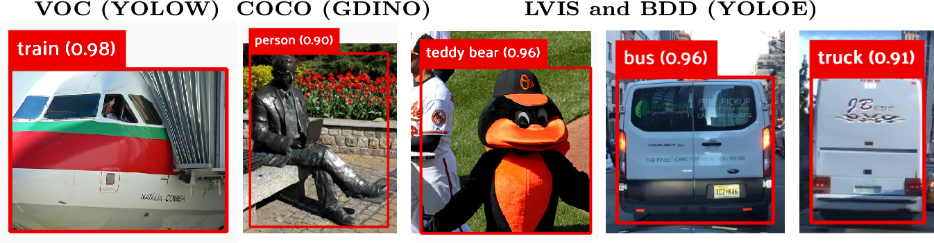
In practice, pseudo-label accuracy is highly variable and, even with high-confidence thresholds, models often produce hallucinations (see 2). Our goal is to (i) selectively prune these inaccurate labels to increase precision, while (ii) preserving accurate labels to maintain recall. Accordingly, we evaluate and prune \(\hat{{\mathbb{Y}}}\) to select label subset \(\tilde{{\mathbb{Y}}} = \{ \tilde{{\boldsymbol{y}}}_i \}^M_{i=1}\) and formulate the pseudo-label pruning problem as \[\begin{align} \mathop{\mathrm{arg\,max}}_{ \tilde{{\mathbb{Y}}} \subseteq \hat{{\mathbb{Y}}}} \mathbb{E}_{{\mathbf{x}}, {\boldsymbol{y}}\sim P} [ F_1 ({\boldsymbol{y}}; \tilde{{\boldsymbol{y}}} )], \\ \end{align} \label{eq:f1}\tag{1}\] where \({\boldsymbol{y}}\) is the ground truth and the \(F_1\) score is the harmonic mean of precision and recall. Specifically, \(F_1 = {\textstyle 2\frac{\text{precision}\cdot\text{recall}}{\text{precision + recall}}} \in [0,1]\), precision \(=\frac{\text{TP}}{\text{TP+FP}}~\in~[0,1]\), recall \(=\frac{\text{TP}}{\text{TP+FN}} \in [0,1]\), true positives (TP) is the number of accurate pseudo-labels, and false negatives (FN) is the number of \({\boldsymbol{y}}\) labels without a corresponding TP. In plain words, precision is the frequency of pseudo-labels being correct, recall is the frequency of ground-truth instances being correctly pseudo-labeled, and the goal of 1 is maximizing the \(F_1\) score, which emphasizes label performance across both metrics (\(F_1=1\) for perfect precision and recall).
Pseudo-labeled datasets are commonly used for downstream model training. However, if left unpruned, pseudo-labels corresponding to hallucinations will induce inductive interference that misleads downstream model convergence. Thus, we combine pruned pseudo-labels \(\tilde{{\mathbb{Y}}}\) with \({\mathbb{D}}_\text{\tiny U}\) to generate the “detoxified” dataset \(\tilde{{\mathbb{D}}} = \{ ({\mathbf{x}}_i, \tilde{{\boldsymbol{y}}}_i) \}^M_{i=1}\). We evaluate \(\tilde{{\mathbb{D}}}\) by reformulating pruning from 1 explicitly for downstream model training as \[\begin{align} \mathop{\mathrm{arg\,min}}_{\tilde{{\mathbb{Y}}} \subseteq \hat{{\mathbb{Y}}} } \mathbb{E}_{{\mathbf{x}}, {\boldsymbol{y}}\sim P} [ \ell ({\mathbf{x}}, {\boldsymbol{y}}; f_{( \tilde{{\mathbb{D}}} )} ) ], \label{eq:downstream} \end{align}\tag{2}\] where \(\ell\) is the task-specific loss function and \(f_{( \tilde{{\mathbb{D}}} )}\) is a model trained on \(\tilde{{\mathbb{D}}}\). In plain words, the goal of 2 is to prune pseudo-labels (\(\tilde{{\mathbb{Y}}}\subseteq \hat{{\mathbb{Y}}}\)) to train a downstream model (\(f\)) that most accurately predicts ground-truth labels (\({\boldsymbol{y}}\)) for unseen images (\({\mathbf{x}}\)) drawn from the underlying data distribution (\(P\)).
4 Adversarial Interrogation via the Label Imitation Game↩︎
The Turing test evaluates a machine’s ability to exhibit intelligent behavior indistinguishable from that of a human [14]. Likewise, our goal is to evaluate which pseudo-labels are indistinguishable from those of a human annotator, implicitly denoting high accuracy. We formalize this as the Label Imitation Game (LIG).
We formulate label tests in the context of a game involving a set of Ideal and Candidate labels and a Judge. The Judge is given all labels and must determine which belong to each set. We use LIG to train the Turing Test Network, which later serves as the Judge at inference to reject and prune pseudo-labels, solving \(\tilde{{\mathbb{Y}}} \subseteq \hat{{\mathbb{Y}}}\) in Eqs. (1 ) & (2 ). We use a tokenized representation (4.1) for the LIG (4.2), but these games are general to the original labels and data.
4.1 Tokenizing Labels & Data↩︎
The transformer architecture (the de facto standard for NLP [34]) operates on a tokenized representation of data to iteratively compare context across all inputs before determining final outputs. To utilize this iterative comparison capability for the LIG, we fuse labels \({\boldsymbol{y}}\) and data \({\mathbf{x}}\) into tokens, specifically \[\begin{align} g ({\mathbf{x}}, {\boldsymbol{y}}) = \{ {\boldsymbol{g}}_1, {\boldsymbol{g}}_2, \dots, {\boldsymbol{g}}_n \}, \\ \end{align} \label{eq:g}\tag{3}\] where \(g\) is a function operating on \({\mathbf{x}}\) and \({\boldsymbol{y}}\), \(n = |{\boldsymbol{y}}|=|g ({\mathbf{x}}, {\boldsymbol{y}})|\), and each output token \({\boldsymbol{g}}_i\) is a lower-dimension representation than \({\mathbf{x}}\) (we specify \(g\) in 5). Extending 3 , we can generate arbitrary tokens across \(m\) data examples as \[{\mathbb{G}}= \{ {\boldsymbol{g}}_1, {\boldsymbol{g}}_2, \dots, {\boldsymbol{g}}_N \} = \{ g ({\mathbf{x}}_i, {\boldsymbol{y}}_i) \}^m_{i=1}. \label{eq:setg}\tag{4}\]
Using 4 , we reformulate label pruning as token pruning, i.e., selecting \(\tilde{{\mathbb{G}}} \subseteq \hat{{\mathbb{G}}}\), where \(\hat{{\mathbb{G}}} = \{ \hat{{\boldsymbol{g}}}_i \}^{\hat{N}}_{i=1} = \{ g ({\mathbf{x}}_i, \hat{{\boldsymbol{y}}}_i) \}^M_{i=1}\) and \(\hat{N}= | \hat{{\mathbb{Y}}} |\). Furthermore, because there is a one-to-one correspondence between tokens and labels, tokens can map directly back to labels as \(g^{-1}: \tilde{{\mathbb{G}}} \rightarrow \tilde{{\mathbb{Y}}}\) in 1 for bijective equivalence.
4.2 Label Imitation Games↩︎
For Game 1, we use 4 to generate a set of tokens \({\mathbb{G}}^* = \{ {\boldsymbol{g}}^*_i \}^{N^*}_{i=1}\) from accurately labeled data \(\{{\mathbf{x}}_i, {\boldsymbol{y}}^*_i \}^{m^*}_{i=1}\) and \(\hat{{\mathbb{G}}} = \{ \hat{{\boldsymbol{g}}}_i \}^{\hat{N}}_{i=1}\) from pseudo-labeled data \(\{ {\mathbf{x}}_i, \hat{{\boldsymbol{y}}}_i \}^m_{i=1}\). The Judge’s objective is to predict which tokens in the combined set correspond to pseudo-labels. We formulate this Pseudo-Label Game as
Game 1 (PLG). Given \({\mathbb{G}}^* \cup \hat{{\mathbb{G}}}\), identify which tokens belong to \(\hat{{\mathbb{G}}}\).
The intuition of PLG is if a Candidate token \(\hat{{\boldsymbol{g}}}_i \in \hat{{\mathbb{G}}}\) is distinguishable from the Ideal set \({\mathbb{G}}^*\), its corresponding pseudo-label is likely inaccurate and should be rejected. Conversely, as \(\hat{{\boldsymbol{g}}}_i\) approaches \({\mathbb{G}}^*\) accuracy, it becomes effectively indistinguishable. In fact, experiments show that carefully chosen \(\hat{{\boldsymbol{g}}}_i\) can even serve as Ideal tokens \({\mathbb{G}}^*\) (we call this “Self-Referential Pruning” in 5.2).
For Game 2, assume each token is associated with a latent category \(c_i \in \mathcal{C}\) from its underlying label and data. Extending 4 , we denote \(c_i \;\forall \;{\boldsymbol{g}}_i\) as \[\label{eq:c} {\mathbb{G}}= \{ {\boldsymbol{g}}^{(c_1)}_1, {\boldsymbol{g}}^{(c_2)}_2, \dots, {\boldsymbol{g}}^{(c_N)}_N \}= \{ g ({\mathbf{x}}_i, {\boldsymbol{y}}_i) \}^m_{i=1}.\tag{5}\] In this game, by construction, the Ideal tokens \({\mathbb{G}}^{(c^*)}\) are homogeneous w.r.t. a target category \(c^*\), s.t. \(c_i = c^*, \forall \;{\boldsymbol{g}}_i^{(c_i)} \in {\mathbb{G}}^{(c^*)}\). Conversely, Candidate tokens \({\mathbb{G}}^{(\neg c^*)}\) are strictly disjoint from \(c^*\), s.t. \(c_i \neq c^*, \forall \;{\boldsymbol{g}}_i^{(c_i)} \in {\mathbb{G}}^{(\neg c^*)}\). The Judge’s objective is to predict which tokens in the combined set belong to disjoint categories \(c_i \neq c^*\). We formulate this Out-of-Category Game as
Game 2 (OCG). Given \({\mathbb{G}}^{(c^*)} \cup {\mathbb{G}}^{(\neg c^*)}\), identify which tokens belong to \({\mathbb{G}}^{(\neg c^*)}\).
Notably, the OCG Judge is not informed of the target category \(c^*\). To ensure the objective is not underdetermined, we implement OCG s.t. \(| {\mathbb{G}}^{(c^*)} | > | {\mathbb{G}}^{(\neg c^*)} |\). This constraint provides sufficient referential density for the Judge to infer target identity, resolve categorical ambiguity, and distinguish the Ideal tokens from Candidates. The intuition of OCG is if a token \({\boldsymbol{g}}_i \in {\mathbb{G}}^{(\neg c^*)}\) is distinguishable from the ideal set \({\mathbb{G}}^{(c^*)}\), its corresponding pseudo-label is semantically inconsistent or noisy and should be rejected. A substantial benefit of OCG is generating numerous training examples for the Turing Test Network (details in 5).
Finally, denoting PLG 1 and or OCG 2 as \(h\), we find \(\tilde{{\mathbb{Y}}} \subseteq \hat{{\mathbb{Y}}}\) in 1 as \[\tilde{{\mathbb{Y}}} = g^{-1}(\tilde{{\mathbb{G}}}) = g^{-1} \big( h ( {\mathbb{G}}^* \cup \hat{{\mathbb{G}}}) \cap \hat{{\mathbb{G}}} \big), \label{eq:h}\tag{6}\] where \(\tilde{{\mathbb{G}}}\) are Candidate pseudo-label tokens \(\hat{{\boldsymbol{g}}}_i \in \hat{{\mathbb{G}}}\) accepted by \(h\) when provided \({\mathbb{G}}^* \cup \hat{{\mathbb{G}}}\) and \(g^{-1}\) maps the tokens back to their original labels (4 ).
5 Learning to Judge: The Turing Test Network↩︎

We introduce the Turing Test Network (TTN) to automate the role of LIG Judge. Specifically, we employ a transformer-based discriminator trained on a LIG-based binary cross-entropy loss to identify label errors (5.1). We train the baseline TTN strictly on classification data but in a class-agnostic manner, withholding categorical labels across 1,303 classes from eight datasets to ensure the TTN learns latent semantic relationships rather than basic class mapping. After training, the TTN exhibits an emergent capacity to build and evaluate semantic (2) and spatial context (3) solely from input sequences, enabling zero-shot transfer to object detection without supervision (5.2). Finally, we introduce a task-specific variant (TTN\(_\text{\tiny D}\)) fine-tuned on detection data, pseudo-labels, and \(\leq 100\) human labels per class for enhanced performance (5.3).
Network Architecture: TTN’s architecture consists of (i) a frozen CLIP [35] feature extractor that encodes label-defined image patches as \({\boldsymbol{f}}_i \in {\mathbb{R}}^{\text{768}}\) and (ii) a custom-learned tokenizer \({\boldsymbol{g}}_i({\boldsymbol{f}}_i) \in {\mathbb{R}}^{\text{512}}\) that enables the (iii) transformer-based reasoning block to evaluate each token and output Accept/Reject logits \(z_i\) (4). For full details, please refer to 8 in the Supplementary Material.
5.1 Training via the Label Imitation Game↩︎
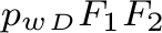
We train the TTN by minimizing a weighted binary cross-entropy (BCE) loss over LIG outcomes. For a sequence of \(n = | {\mathbb{G}}|\) tokens, the objective function is \[\mathcal{L}_\text{\tiny BCE}({\boldsymbol{w}}) := - \sum_{i=1}^{n} \Big[ p_w y_i \cdot \log \big( \sigma (z_i) \big) + (1-y_i) \cdot \log \big(1 - \sigma(z_i) \big) \Big], \label{eq:loss}\tag{7}\] where \({\boldsymbol{w}}\) are trainable parameters of the tokenizer and transformer, \(y_i \in \{0,1\}\) is the ground-truth indicator assigning \(y_i = 0\) to the Accept set and \(y_i=1\) to the Reject set, \(p_w\) is a positive weight applied to Reject training examples (conceptually, pruning aggression), \(z_i\) is the output logit per token \({\boldsymbol{g}}_i \in {\mathbb{G}}\), and \(\sigma(z_i) = \frac{1}{1 + e^{-z_i}}\) is the model’s estimated probability that \({\boldsymbol{g}}_i\) should be rejected.

To ensure the TTN generalizes across diverse failure modes, we construct training batches by sampling tokens \({\boldsymbol{g}}_i\) from a categorical training distribution \(P({\mathbb{S}})\) over the following four mutually exclusive states \({\mathbb{S}}\in \{1,2,3,4\}\):
\({\mathbb{S}}=\)a\(1\) (Ideal): High-fidelity human-label token with target category \(c^*\).
\({\mathbb{S}}=~\) \(2\) (OCG-Human): Human-label token with disjoint category \(c_i \neq c^*\).
\({\mathbb{S}}=~\) \(3\) (OCG-Pseudo): Pseudo-label token with disjoint category \(c_i \neq c^*\).
\({\mathbb{S}}=~\) \(4\) (PLG): Pseudo-label token of any fidelity and target category \(c^*\).
By construction, \(y_i=1\) if \({\mathbb{S}}=1\) and \(y_i=0\) otherwise in 7 . We denote the sampling probability for each state as \(\pi_k = P({\mathbb{S}}=k)\), where \(\sum \pi_k =1\). This formulation enables control of LIG difficulty by adjusting the training failure distribution. For OCG (\({\mathbb{S}}= \{2,3\}\)), all disjoint categories \(c_i \neq c^*\) have an equal chance of being selected, but we only use one disjoint category per game.
Training Protocol: Each training sequence includes references for context prior to candidates. Specifically, we assign the first 10 positions sampled exclusively from the Ideal state (\({\mathbb{S}}=1\)) to the Reference Set. To ensure a robust reference context, we limit Reference Sets to only include categories with \(N > 10\) instances. The final position is reserved for the Candidate Slot, which is sampled from the full distribution \(P({\mathbb{S}})\). This forces the TTN to utilize the Reference Set’s context to interrogate the Candidate’s fidelity. While experiments indicate the TTN can handle an arbitrary number of Reference and Candidate Slots, we utilize this 10:1 ratio for all training results. Notably, a disjoint category may still serve as a Reject Candidate (\({\mathbb{S}}\neq 1\)) even if it fails to meet the Reference Set threshold (i.e., \(N \leq 10\) instances), provided it contains at least one representative label.
Optimization: We optimize the baseline TTN using \(p_w=1\) in 7 , a batch size of 256, and an SGD optimizer (\(5 \times 10^{-4}\) weight decay, \(5 \times 10^{-3}\) learning rate, implemented via PyTorch [36]). Each distinct dataset contributes 1,000 training sequences per epoch, with a 20% held-out validation set for model selection. To ensure the TTN is a balanced and domain-agnostic judge, we select the final parameters \({\boldsymbol{w}}\) from the checkpoint achieving the highest validation accuracy. Specifically, we evenly weight the Accept (\({\mathbb{S}}= 1\)) and Reject (\({\mathbb{S}}\neq 1\)) accuracies per dataset, then average across all datasets in ¿tbl:tab:icdataset?. This dual-averaging strategy prevents the TTN from over-fitting to specific image domains or majority-class distributions. Notably, rotating disjoint categories \(c_i \neq c^*\) evenly within each dataset also reduces memorizing specific features for the 1,303 overall classes. The TTN trains for 100K epochs (hold-out selection at the 90K checkpoint) in 61.05 hours on a single NVIDIA L40S GPU. This modest computational requirement—relative to the foundation models it evaluates—highlights TTN efficiency as a general lightweight pruning module.
5.2 Zero-Shot Cross-Task Transfer↩︎
| c | r | r | c | r | r | c | & & &
Dataset & & & & & &
ImageNet [37] & 1,000 & 1,281,167 & Varied & 97.7% & 94.8% & 96.2%
Food-101 [38] & 101 & 101,000 & \(\leq\)512 & 97.7% & 95.3% & 96.5%
CIFAR100 [39] & 100 & 50,000 & 32\(\times\)32 & 77.6% & 85.4% & 81.5%
MIT Indoor Scenes [40] & 67 & 15,620 & \(\geq\)200 & 98.9% & 96.5% & 97.7%
Fashion-MNIST [41] & 10 & 60,000 & 28\(\times\)28 & 97.2% & 92.5% & 94.8%
CIFAR10 [39] & 10 & 50,000 & 32\(\times\)32 & 98.3% & 97.8% & 98.0%
EuroSAT [42] & 10 & 27,000 & 64\(\times\)64 & 98.6% & 97.6% & 98.1%
VTID2 [43] & 5 & 4,356 & Varied & 100.0% & 99.8% & 99.9%
TTN’s zero-shot cross-task transfer performance—pruning object detection labels with a model trained purely on image classification (1 2 3 4)—stems directly from our training protocol, which forces the TTN to identify robust semantic boundaries purely from diverse, high-fidelity input sequences (¿tbl:tab:icdataset?). Specifically, the TTN training sampling distribution \(P({\mathbb{S}})\) uses only human-verified sources, \(\pi_\text{\ref{s:1}}=\pi_\text{\ref{s:2}}=\frac{1}{2}\), with zero pseudo-label probabilities, \(\pi_\text{\ref{s:3}}=\pi_\text{\ref{s:4}}=0\). By excluding noisy pseudo-labels and detection-specific formats during this phase, we ensure the TTN internalizes a robust intrinsic semantic logic. This foundation generalizes to novel tasks and categories in a zero-shot manner, requiring no task-specific supervision. Furthermore, including low-resolution datasets (e.g., CIFAR, Fashion-MNIST) acts as an inherent curriculum for scale variation.
TTN LIG Evaluation: As detailed in ¿tbl:tab:icdataset?, the TTN achieves high validation accuracy (\(>94\%\) Overall on 7/8 datasets) across diverse classification domains. Notably, the model maintains robust performance even on low-resolution data (e.g., 98.0% on CIFAR10), which is representative of the visual degradations typical of tiny object pseudo-labels. By learning to judge pixelated and high-fidelity labels for numerous classes, the TTN develops a domain-agnostic semantic logic that facilitates effective zero-shot transfer from classification to detection.
Self-Referential Pruning: After foundation model pseudo-labeling, the TTN prunes detection labels without human supervision by constructing a dataset-spanning “Ideal” set from the 1,000 highest-confidence pseudo-labels per target category \(c^*\), \(|{\mathbb{G}}^{(c^*)}| \leq 1,000\). We then perform a Self-Referential LIG for each category, where the TTN evaluates every pseudo-label candidate \(\hat{{\boldsymbol{g}}}_i^{(c^*)} \in \hat{{\mathbb{G}}}^{(c^*)}\) (including “Ideal” selections) against 10 reference samples drawn from \({\mathbb{G}}^{(c^*)}\). We aggregate the Accept/Reject logits for each candidate (\(z_i\)) across multiple games to cover all available references and increase robustness; if a candidate’s aggregate score is \(>0\), it is pruned (6 ). This iterative process allows the TTN to identify and reject systemic hallucinations, even if they had high initial confidence (2). Categories lacking sufficient reference labels (\(|{\mathbb{G}}^{(c^*)}| < 10\)) are preserved with their original pseudo-labels to prevent uncontextualized pruning.
5.3 Task-Specific Fine-Tuning↩︎
| c | r | r | r | c | r | r | c | & & Objects &
Dataset & & & & per Image & & &
VOC [44] & 20 & 16,551 & 40,058 & 2.42 & 95.1% & 84.2% & 89.7%
COCO [45] & 80 & 118,287 & 849,945 & 7.19 & 96.8% & 59.2% & 78.0%
LVIS [46] & 1,203 & 100,170 & 1,270,141 & 12.68 & 95.8% & 50.6% & 73.2%
BDD [47] & 10 & 70,000 & 1,286,871 & 18.38 & 93.0% & 63.0% & 78.0%
To maximize detection pruning performance, we test task-specific fine-tuning (TTN\(_\text{\tiny D}\)) with the full LIG training sampling distribution \(P({\mathbb{S}})\). From TTN weights, we fine-tune a single TTN\(_\text{\tiny D}\) model on all detection datasets in ¿tbl:tab:detectdataset? simultaneously, spanning web images to autonomous driving. This multi-domain approach ensures \(\text{TTN}_{\text{\tiny D}}\) is a robust generalist across diverse visual contexts while mastering the specific spatial and semantic nuances of the object detection task.
For the Ideal set (\({\mathbb{S}}= \;\)[s:1]), TTN\(_\text{\tiny D}\) uses up to 100 human-verified detection labels for each target category (subject to availability), which are split 80/20 for the train/validation protocol. For label efficiency, the 80 training labels are reused as the Ideal set for pseudo-label pruning at inference (\(|{\mathbb{G}}^{(c^*)}| \leq 80\)).
To generate the remaining training distributions (\({\mathbb{S}}=\{2,3,4\}\)), TTN\(_\text{\tiny D}\) uses three Vision-Language Models (VLMs): YOLO-World (YOLOW) [18], YOLOE [48], and Grounding DINO-Tiny (GDINO) [17], each sampled at a confidence threshold of \(\tau=0.1\). To maximize the hallucination signal relative to the Ideal set, we limit training examples from each VLM to the lowest-confidence quartile of pseudo-labels per class. Each VLM-dataset combination contributes 1,000 training sequences per epoch, exposing TTN\(_\text{\tiny D}\) to the diverse error characteristics and spatial inaccuracies of multiple VLM architectures.
TTN\(_\text{\tiny D}\) adopts the baseline TTN training configuration with three modifications: (i) a non-uniform sampling distribution of \(\pi_\text{\ref{s:1}}=\frac{1}{2}\), \(\pi_\text{\ref{s:2}}=\frac{1}{4}\), \(\pi_\text{\ref{s:3}}=\pi_\text{\ref{s:4}}=\frac{1}{8}\); (ii) a reduced pruning aggression (\(p_w=0.2\) in 7 ) to instill a conservative bias that minimizes false rejections, ensuring the TTN\(_\text{\tiny D}\) only prunes when there is strong evidence of a hallucination; and (iii) a 0.02 learning rate for 4K epochs (with selection at the 2K checkpoint), requiring only 4.28 hours of fine-tuning.
After fine-tuning, \(\text{TTN}_{\text{\tiny D}}\) achieves high validation accuracies (73–90%, ¿tbl:tab:detectdataset?). Accept accuracy (Candidate \({\mathbb{S}}=1\)) consistently exceeds 93% across all domains. Reject accuracy (\({\mathbb{S}}=\{2,3,4\}\)) naturally reflects the varying instance density and class complexity of the target datasets, which we explore further in 6.
6 Experimental Evaluation of the LIG and TTN↩︎
6.1 Experimental Setup↩︎
Our experimental setup is motivated by the comprehensive Auto-Labeling (AL) benchmark [11]. This foundation model pseudo-labeling benchmark uses GDINO, YOLOE, and YOLOW VLMs across various confidence thresholds \(\tau\) and four diverse detection datasets: VOC, COCO, LVIS, and BDD. We use \(\tau \in [0.05, 0.5]\) to improve peak AL \(F_1\)-score performance via TTN pruning (\(\tilde{{\mathbb{Y}}} \subseteq \hat{{\mathbb{Y}}}\) in 1 ). The AL benchmark includes training downstream detectors strictly on pseudo-labels, which provides another evaluation for TTN performance gains (\(\tilde{{\mathbb{D}}}\) in 2 ). In addition to TTN, we include LIG\(^*\) as an Oracle judge that prunes all candidate pseudo-labels with \(\text{IoU}<0.5\). This represents an IoU-specific upper bound for LIG-based pruning, though it preserves spatial label redundancies. See Supplementary Material for method comparisons, ablations, runtime, extended benchmark results, and full experiment details ([sec:ablate] [sec:compare] [sec:compute] [sec:supexp] [sec:supsetup]).
6.2 Interrogating the Signal: Pseudo-Label Evaluation↩︎

We first evaluate the effectiveness of the TTN as a standalone pseudo-label filter. As shown on VOC in 5, TTN consistently improves precision across all VLM models and confidence thresholds. While pruning naturally results in an incidental decrease in recall, the more substantial precision increases lead to overall \(F_1\)-score improvements across all datasets (¿tbl:tab:metricmap?). Specifically, TTN and TTN\(_\text{\tiny D}\) improve Overall \(F_1\) by 4% and 7%, respectively, advancing toward the 45% gain set by the LIG\(^*\) Oracle. Notably, LIG\(^*\) exhibits an epsilon improvement in recall due to matching disambiguation. Essentially, by rejecting high-entropy labels, we reduce Hungarian matching interference and enable higher-fidelity pairings between the accepted pseudo-labels and ground truth during evaluation.
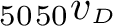
We also evaluate the \(F_2\) score, which favors recall (\(\frac{\text{5TP}}{\text{5TP+4FN+FP}}\)\(\in[0,1]\)), to measure the trade-off between pruning and signal preservation. TTN\(_\text{\tiny D}\) improves Overall \(F_2\) by 3%, demonstrating that its task-specific logic “detoxifies” the label set while preserving high-recall candidates for downstream training.
| c| l | r |c | c | c | c| c| c| & &
Dataset & & & & & & & &
& LIG\(^*\) & 39,008 & 0.816 & 0.914 & 0.845 & 0.825 & 0.707 & 0.500
& TTN\(_{\text{\tiny D}}\) & 61,337 & 0.788 & 0.677 & 0.695 &0.734 & 0.685 & 0.486
VOC & TTN & 78,403 & 0.794 & 0.628 & 0.662 & 0.716 & 0.675 & 0.478
& AL [11] & 134,899 & 0.815 & 0.562 & 0.615 & 0.690 & 0.656 & 0.466
& LIG\(^*\) & 627,792 & 0.594 & 0.908 & 0.689 & 0.626 & 0.454 & 0.315
& TTN\(_{\text{\tiny D}}\) & 1,565,002 & 0.582 & 0.537 & 0.511 & 0.534 & 0.436 & 0.302
COCO & TTN & 1,192,383 & 0.538 & 0.571 & 0.513 & 0.515 & 0.434 &0.303
& AL & 1,834,962 & 0.593 & 0.514 & 0.499 & 0.531 & 0.432 & 0.299
& LIG\(^*\) & 290,613 & 0.137 & 0.600 & 0.191 & 0.154 & 0.059 & 0.041
& TTN\(_{\text{\tiny D}}\) & 1,659,673 & 0.136 & 0.116 & 0.079 & 0.087 & 0.060 & 0.042
LVIS & TTN & 1,508,817 & 0.131 &0.116 &0.079 & 0.086 & 0.059 & 0.042
& AL & 1,777,051 & 0.137 & 0.112 & 0.078 & 0.087 & 0.059 & 0.042
& LIG\(^*\) & 426,726 & 0.267 & 0.837 & 0.376 & 0.301 & 0.306 & 0.178
& TTN\(_{\text{\tiny D}}\) & 773,755 & 0.243 & 0.459 & 0.262 & 0.235 & 0.269 & 0.156
BDD & TTN & 854,393 & 0.242 & 0.428 & 0.249 & 0.227 & 0.252 & 0.148
& AL & 1,084,056 & 0.267 & 0.411 & 0.256 & 0.241 & 0.253 & 0.147
& LIG\(^*\) & 346,035 & 0.454 & 0.815 & 0.525 & 0.476 & 0.382 & 0.259
& TTN\(_{\text{\tiny D}}\) & 1,014,942 & 0.437 & 0.447 & 0.387 & 0.398 & 0.362 & 0.247
Overall & TTN & 908,499 & 0.426 & 0.436 & 0.376 & 0.386 & 0.355 & 0.243
& AL & 1,207,742 & 0.453 & 0.400 & 0.362 & 0.387 & 0.350 & 0.238
6.3 Detector Training and Evaluation on Detoxified Labels↩︎
We further evaluate the utility of our pruning framework by training downstream object detectors on the detoxified pseudo-labeled datasets. Specifically, for each dataset, we train a YOLO11n detector [49] on unlabeled training images paired with TTN-pruned pseudo-labels (\(\tilde{{\mathbb{D}}}\) in 2 ). After training, these detectors are then evaluated on their respective human-labeled validation sets. Critically, these validation sets (both images and labels) are entirely disjoint and unseen by both the TTN and the downstream detectors, ensuring a robust measure of how TTN pruning improves generalization from VLM supervision.
As shown in ¿tbl:tab:metricmap?, training on TTN-pruned datasets results in consistent mAP\(_{50}\) and mAP\(_{50:95}\) improvements across all VLM architectures and datasets. Remarkably, although TTN\(_\text{\tiny D}\) does not reject nearly as many pseudo-labels as the LIG\(^*\) Oracle (see Labels in ¿tbl:tab:metricmap?), TTN\(_\text{\tiny D}\) closes 38% of the mAP\(_{50}\) and 43% of the mAP\(_{50:95}\) gap between AL and LIG\(^*\) performance. This indicates that TTN\(_\text{\tiny D}\) successfully rejects many of the VLM hallucinations that are particularly disruptive for downstream training. As illustrated in 6, mAP\(_{50}\) gains are particularly pronounced at lower confidence thresholds (\(\tau\)). By detoxifying the low-\(\tau\), high-recall regime, the TTN effectively expands the usable training distribution, allowing the downstream detector to learn from a larger, yet cleaner, set of examples. With TTN’s generalization across categories established, we focus on the most challenging, transfer-vulnerable classes in 6.4.
6.4 Category Revival: Rescuing Vulnerable Classes↩︎
To understand TTN performance on challenge categories, we perform a targeted evaluation for AL’s [11] maximum and non-zero minimum \(F_1\)-score classes in 1. While TTN \(F_1\) gains are consistent across VLM models and datasets for the Max. \(F_1\) classes, gains for the challenge classes are particularly significant (e.g., \(>300\%\) for GDINO Chair). For the Min. \(F_1\) class mean, specifically, zero-shot TTN increases \(F_1\) by 28% and TTN\(_\text{\tiny D}\) increases \(F_1\) by 44%, effectively “raising the floor” for VLM-driven labeling. Remarkably, LIG\(^*\) Oracle pruning increases Min. \(F_1\) by 432%, indicating systemic VLM hallucinations that would have induced severe inductive interference in downstream models.
| VOC \(F_1\) | COCO \(F_1\) | BDD \(F_1\) | ||||||||
| GDINO | YOLOE | YOLOW | GDINO | YOLOE | YOLOW | GDINO | YOLOE | YOLOW | Mean | |
| Cat | Cat | Cat | Cat | Bear | Giraffe | Car | Car | Person | ||
| LIG\(^*\) | 0.747 | 0.940 | 0.948 | 0.675 | 0.892 | 0.935 | 0.693 | 0.577 | 0.656 | 0.785 |
| TTN\(_{\text{\tiny D}}\) | 0.687 | 0.907 | 0.915 | 0.602 | 0.819 | 0.873 | 0.478 | 0.519 | 0.545 | 0.705 |
| TTN | 0.649 | 0.893 | 0.903 | 0.579 | 0.848 | 0.878 | 0.443 | 0.479 | 0.518 | 0.688 |
| AL [11] | 0.585 | 0.822 | 0.851 | 0.528 | 0.784 | 0.861 | 0.438 | 0.535 | 0.543 | 0.661 |
| Chair | Chair | Sofa | Handbag | Toaster | Toaster | Train | Motor | Train | ||
| LIG\(^*\) | 0.641 | 0.892 | 0.940 | 0.516 | 0.840 | 0.686 | 0.323 | 0.018 | 0.319 | 0.575 |
| TTN\(_{\text{\tiny D}}\) | 0.204 | 0.520 | 0.436 | 0.047 | 0.194 | 0.186 | 0.005 | 0.016 | 0.116 | 0.192 |
| TTN | 0.172 | 0.489 | 0.391 | 0.051 | 0.180 | 0.175 | 0.002 | 0.014 | 0.058 | 0.170 |
| AL | 0.054 | 0.364 | 0.319 | 0.045 | 0.174 | 0.166 | 0.002 | 0.016 | 0.058 | 0.133 |
| c| l | r |c | c | c | c| c| c| & &
Dataset & & & & & & & &
& LIG\(^*\) & 7,340 & 0.716 & 0.898 & 0.760 & 0.729 & 0.522 & 0.328
& TTN\(_{\text{\tiny D}}\) & 19,265 & 0.682 & 0.513 & 0.512 & 0.576 & 0.485 & 0.308
VOC\(_v\) & TTN & 22,084 & 0.686 & 0.483 & 0.490 & 0.562 & 0.470 & 0.300
& AL [11] & 47,139 & 0.715 & 0.425 & 0.442 & 0.528 & 0.438 & 0.281
& LIG\(^*\) & 89,503 & 0.422 & 0.898 & 0.545 & 0.461 & 0.204 & 0.124
& TTN\(_{\text{\tiny D}}\) & 446,132 & 0.413 & 0.392 & 0.338 & 0.355 & 0.184 & 0.112
COCO\(_v\) & TTN & 319,843 & 0.380 & 0.410 & 0.340 & 0.345 & 0.185 & 0.113
& AL & 544,203 & 0.421 & 0.381 & 0.333 & 0.353 & 0.175 & 0.106
& LIG\(^*\) & 266 & 0.027 & 0.269 & 0.045 & 0.032 & 0.0004 & 0.0003
& TTN\(_{\text{\tiny D}}\) & 27,025 & 0.027 & 0.034 & 0.013 & 0.014 & 0.0007 & 0.0006
LVIS\(_v\) & TTN & 29,297 & 0.026 & 0.032 & 0.013 & 0.013 & 0.0009 & 0.0007
& AL & 31,402 & 0.027 & 0.032 & 0.012 & 0.014 & 0.0007 & 0.0006
& LIG\(^*\) & 453 & 0.077 & 0.576 & 0.123 & 0.091 & 0.036 & 0.016
& TTN\(_{\text{\tiny D}}\) & 18,535 & 0.075 & 0.074 & 0.035 & 0.042 & 0.013 & 0.006
BDD\(_v\) & TTN & 32,899 & 0.076 & 0.035 & 0.022 & 0.031 & 0.006 & 0.003
& AL & 34,888 & 0.077 & 0.036 & 0.022 & 0.032 & 0.007 & 0.003
& LIG\(^*\) & 24,390 & 0.311 & 0.660 & 0.368 & 0.328 & 0.191 & 0.117
& TTN\(_{\text{\tiny D}}\) & 127,739 & 0.299 & 0.253 &0.225 &0.247 &0.171 &0.107
Overall\(_v\) & TTN & 101,031 & 0.292 & 0.240 & 0.216 & 0.238 & 0.166 & 0.104
& AL & 164,408 & 0.310 & 0.218 & 0.202 & 0.231 & 0.155 & 0.098
Motivated by this finding, we perform a broader analysis of these challenge categories in downstream model training. Specifically, we evaluate transfer-vulnerable classes (\(v\)), defined per-VLM as the bottom quartile of classes ranked by AL’s [11] downstream mAP\(_{50}\) at \(\tau=0.1\). As shown in 6, TTN pruning consistently improves mAP\(_{50}\) across confidence thresholds and datasets on these failing categories. Remarkably, TTN\(_\text{\tiny D}\) approximately doubles precision, \(F_1\), mAP\(_{50}\), and mAP\(_{50:95}\) on BDD\(_v\) with only a 3% reduction in recall after pruning 53% of the labels, as shown in ¿tbl:tab:metricmapv?. Across all datasets, zero-shot TTN and TTN\(_\text{\tiny D}\) improve Overall mAP\(_{50:95}\) by 6% and 9%, respectively.
By selectively pruning disruptive candidates, both TTNs facilitate a particularly striking Category Revival, where the downstream model achieves non-trivial mAP on classes that previously exhibited zero recall. For example, at a \(\tau=0.1\) threshold on LVIS, the AL baseline exhibits 0 recall for the 259 vulnerable classes regardless of VLM. The zero-shot TTN recovers recall for 37 of these categories (27, 10 for YOLOE, YOLOW), while \(\text{TTN}_{\text{\tiny D}}\) recovers 28 (17, 11 for YOLOE, YOLOW). This disproportionate improvement suggests that many transfer-vulnerable classes do not suffer from a lack of data, but rather from an exceptionally high noise-to-signal ratio. This recovery of the most challenging classes shows that the TTN’s semantic pruning is a critical component for achieving robust generalization in fully autonomous pseudo-labeling pipelines.

7 Conclusion and the Post-Engine Interrogation Frontier↩︎
In this paper, we introduced the Label Imitation Game (LIG), a Turing-inspired framework that formalizes pseudo-label pruning as a dataset-wide adversarial interrogation. By developing the Turing Test Network (TTN), we demonstrate that a model trained strictly on image classification can effectively judge and “detoxify” complex object detection pseudo-labels. Our experiments across four diverse datasets show that the TTN successfully suppresses systemic foundation model hallucinations, yielding zero-shot \(F_1\)-score gains of 28% for the most challenging categories—rising to 44% with task-specific fine-tuning (\(\text{TTN}_{\text{\tiny D}}\)). Crucially, both models facilitate Category Revival, enabling downstream detectors to recover from zero recall on dozens of transfer-vulnerable classes. Our results establish that global semantic-contextual logic is a robust alternative to local spatial-geometric verification. By releasing our LIG framework and pre-trained TTN weights, we provide the vision community with a lightweight, task-agnostic module that enhances pseudo-labeling rigor at scale.
Looking forward, a significant Post-Engine Interrogation Frontier remains for future work. As shown in 7, the optimal pruning regime includes low-confidence labels, where the most authentic signal is often discarded by traditional filtering. \(\text{TTN}_{\text{\tiny D}}\) substantially narrows this performance gap, but additional gains must be won from increasingly subtle and difficult-to-identify hallucinations. We postulate that integrating multi-model consensus and LIG-aware spatial redundancy reduction will close this gap. To broaden applicability, expanding the TTN’s interrogative capacity to video [50] and 3D modalities [51] provides new frontiers for fully autonomous, noise-robust machine learning.
Supplementary Material
The Label Imitation Game: Turing Test Network for Zero-Shot Pseudo-Label Pruning
Brent A. Griffin and Jason J. Corso
Contents of the Supplementary Material↩︎
Section 8: Network Architecture Specifications
Section 9: Extended Method Comparisons
Section 10: Methodological Validation and Sensitivity Analysis
Section 11: Computational Efficiency & Scalability
Section 12: Extended Performance Benchmarks
Section 13: Experimental Protocol
8 Network Architecture Specifications↩︎
To elaborate on 5, we provide the full architectural details of the Turing Test Network (TTN), which consists of three stages: a frozen feature extractor, a custom-learned tokenizer, and a transformer-based reasoning block. These architectural designs enable the TTN to build and evaluate semantic and spatial context without class labels, thus facilitating zero-shot transfer (8).

8.1 Stage 1: Frozen Feature Extractor↩︎
TTN uses a pre-trained vision-language model to establish a high-level semantic representation of labels. Specifically, we use the CLIP ViT-L/14 model [35] to encode the underlying image patches defined by each label. We keep the encoder frozen for a robust, general-purpose initial feature space \({\boldsymbol{f}}_i \in {\mathbb{R}}^{\text{768}}\).
8.2 Stage 2: Custom-Learned TTN Tokenizer↩︎
To bridge the gap between static CLIP embeddings and the transformer reasoning space, a lightweight multi-layer perceptron (MLP) transforms the initial features into “TTN Tokens.” The MLP sequentially processes \({\boldsymbol{f}}_i\) through a fully-connected 1,024-D layer, a ReLU activation, a fully-connected 512-D layer, and, finally, a Dropout layer (\(p=0.2\)). The output tokens \({\boldsymbol{g}}_i({\boldsymbol{f}}_i) \in {\mathbb{R}}^{\text{512}}\) (3 ) are the condensed visual and semantic information TTN evaluates during the Label Imitation Game (LIG).
8.3 Stage 3: Non-Masked Transformer-based Reasoning Block↩︎
The core of TTN is an eight-layer transformer that evaluates each token \({\boldsymbol{g}}_i \in {\mathbb{G}}\). Unlike standard classifiers that process examples in isolation, this block utilizes non-masked Multi-Head Self-Attention (MHSA) to evaluate many tokenized labels across an arbitrary number of data examples simultaneously (4 ). To preserve relational and sequential context across tokens, we add learned positional encodings via an embedding table to the transformer input. The MHSA block splits the input tokens into eight heads, while the subsequent feed-forward block reuses the tokenizer’s MLP design with new weights. To ensure stable gradient flow, each transformer layer has residual connections where the input is normalized only for sub-layer operations and added to each sub-layer output. The final output state of each token is passed through a final layer normalization and linear projection layer to produce the Accept/Reject logits (\(z_i\) in 7 ).
9 Extended Method Comparisons↩︎
We provide additional method comparisons to supplement the related work (2) and experimental evaluation (6) of the main paper. To provide more context for related work, we compare the methodological setup and procedural requirements for several representative methods in [tbl:tab:method]. Importantly, only TTN and the AL baseline are zero-shot compatible with existing object detection frameworks. All other methods require ground-truth detection labels or, more commonly, invasive changes to the underlying model architecture, training pipeline, or even the core methodology itself for detection compatibility.
4.4pt
| l | c | c | c | & Developed &
& for Object & & Detection
& Detection & &
AL [11], TTN & Yes & Yes & Yes
CLIP kNN Prune, TTN\(_{\text{\tiny D}}\) & Yes & Yes & No
SoftTeacher [52] & Yes & No & No
Co-teaching [13], FixMatch [21], & & &
kNN-CLIP [53], MentorNet [12] & No & No & No
To expand the method evaluation in 6, following kNN-CLIP [53], we implement kNN baselines that prune or relabel pseudo-labels based on the majority-vote consistency among the 16 nearest ground-truth CLIP embeddings (using \(\leq\) 100 ground-truth labels per class). We also implement kNN baselines with TTN Token embeddings (\({\boldsymbol{g}}_i({\boldsymbol{f}}_i) \in {\mathbb{R}}^{\text{512}}\) in 8.2) to compare their label pruning efficacy directly against the frozen CLIP embeddings (\({\boldsymbol{f}}_i \in {\mathbb{R}}^{\text{768}}\) in 8.1). As shown in ¿tbl:tab:compare?, both TTN and TTN\(_\text{\tiny D}\) Token-based kNN outperform CLIP, which supports the decision to include the TTN Tokenizer in the full TTN architecture (see 8). Furthermore, while TTN Token and CLIP kNN pruning outperform the AL baseline, zero-shot pruning with the full TTN architecture and corresponding semantic logic surpasses all kNN baselines despite their use of ground-truth labels. Notably, CLIP kNN relabeling decreases AL performance, which further motivates our focus on pruning-based approaches.
5.4 pt
| l | c | c | c | c | c | c | & & GT &
& Label & Labels &
Method & Operation & per Class & & & &
& Prune & \(\leq\) 100 & 0.437 & 0.447 & 0.387 & 0.398
& Prune & zero-shot & 0.426 & 0.436 & 0.376 & 0.386
TTN\(_{\text{\tiny D}}\) Token kNN & Prune & \(\leq\) 100 & 0.367 & 0.508 & 0.373 & 0.360
TTN Token kNN & Prune & \(\leq\) 100 & 0.357 & 0.512 & 0.367 & 0.352
CLIP kNN & Prune & \(\leq\) 100 & 0.347 & 0.523 & 0.366 & 0.346
AL& – & zero-shot & 0.453 & 0.400 & 0.362 & 0.387
CLIP kNN & Relabel & \(\leq\) 100 & 0.402 & 0.285 & 0.275 & 0.312
10 Methodological Validation and Sensitivity Analysis↩︎
To quantitatively validate design decisions from the main paper, we include supplementary results for methodological ablations and sensitivity analyses in 9 and ¿tbl:tab:ablate?. While TTN is robust to many variations, ablations show TTN’s chosen pruning aggression (\(p_w=1\)), sample distribution (\(\pi_\text{1,2}=\frac{1}{2}\)), token design (\({\boldsymbol{g}}_i \in {\mathbb{R}}^{512}\)), and number of input tokens (10 Reference, 1 Candidate) enable TTN to train from scratch on classification data then perform zero-shot pruning on detection labels with high \(F_1\) and \(F_2\) scores. Notably, training TTN from scratch with the lowest pruning aggression (\(p_w=0.1\)) causes TTN to simply accept all labels, which results in identical performance to the AL baseline.
| l | l | c | c | c | c | & &
& &
Method & & & & &
& \(\pi_\text{1}=\frac{1}{2}\), \(\pi_\text{2}=\frac{1}{4}\), \(\pi_\text{3,4}=\frac{1}{8}\) & 0.437 & 0.447 & 0.387
& 0.398
TTN\(_{\text{\tiny D}}\) & OCG-Pseudo \(\pi_\text{1,3}=\frac{1}{2}\), \(\pi_\text{2,4}=0\) & 0.431 & 0.451 & 0.385
& 0.394
TTN\(_{\text{\tiny D}}\) & Uniform \(\pi_\text{1,2,3,4}=\frac{1}{4}\) & 0.439 & 0.442 & 0.384 & 0.396
TTN\(_{\text{\tiny D}}\) & OCG-Human \(\pi_\text{1,2}=\frac{1}{2}\), \(\pi_\text{3,4}=0\) & 0.434 & 0.441 & 0.380
& 0.393
TTN\(_{\text{\tiny D}}\) & PLG \(\pi_\text{1,4}=\frac{1}{2}\), \(\pi_\text{2,3}=0\) & 0.408 & 0.459 & 0.372
& 0.376
& \(\pi_\text{1,2}=\frac{1}{2}\), \(\pi_\text{3,4}=0\) & 0.426 & 0.436 & 0.376 & 0.386
TTN & \(\pi_\text{1}=\frac{1}{4}\), \(\pi_\text{2}=\frac{3}{4}\), \(\pi_\text{3,4}=0\) & 0.415 & 0.442 & 0.374 & 0.381
TTN & \(\pi_\text{1}=\frac{3}{4}\), \(\pi_\text{2}=\frac{1}{4}\), \(\pi_\text{3,4}=0\) & 0.385 & 0.467 & 0.373 &
0.366
& \(n=\) 512 & 0.426 & 0.436 & 0.376 & 0.386
TTN & \(n=\) 256 & 0.424 & 0.438 & 0.376 & 0.385
TTN & \(n=\) 1,024 & 0.387 & 0.447 & 0.365 & 0.363
TTN & 10 Reference, 2 Candidate & 0.406 & 0.455 & 0.377 & 0.378
& 10 Reference, 1 Candidate & 0.426 & 0.436 & 0.376 & 0.386
TTN & 20 Reference, 1 Candidate & 0.399 & 0.454 & 0.373 & 0.373
TTN & 5 Reference, 1 Candidate & 0.404 & 0.437 & 0.367 & 0.372
TTN & 10 Reference, 5 Candidate & 0.382 & 0.441 & 0.357 & 0.357
TTN & \(\leq\) 80 GT Reference (100%) & 0.442 & 0.427 & 0.379 & 0.395
& \(\leq\) 1,000 Self-Referential (63.6%) & 0.426 & 0.436 & 0.376 & 0.386
TTN & \(\leq\) 100 Self-Referential (70.9%)& 0.414 & 0.448 & 0.376 & 0.381
Subsequent to TTN training, the pruning reference set ablations in ¿tbl:tab:ablate? reveal a trade-off. Reducing the self-referential pruning set size from \(\le\) 1,000 to \(\le\) 100 highest-confidence samples improves the reference set’s accuracy (\(63.6\% \rightarrow 70.9\%\)) but degrades final pruning performance (\(0.386 \rightarrow 0.381~F_2\) score) due to a reduction in contextual breadth. However, if available, using \(\le\) 80 higher-quality ground-truth labels bridges this contextual gap, enabling TTN to approach the pruning performance of fine-tuned TTN\(_\text{\tiny D}\) (3.95 and 3.98 \(F_2\) scores respectively).
For fine-tuned TTN\(_\text{\tiny D}\), increasing \(p_w\) increases precision but also decreases recall, with the chosen \(p_w=0.2\) achieving the highest \(F_2\) score in 9. TTN\(_\text{\tiny D}\) train distribution ablations reveal that OCG-Pseudo (\(\pi_3\)) is the best individual game—followed by OCG-Human and PLG—yet the nominal TTN\(_{\text{\tiny D}}\) performs best in ¿tbl:tab:ablate?, validating that using all games is optimal.
11 Computational Efficiency & Scalability↩︎
To establish the computational efficiency and scalability of TTN pruning, we provide a runtime comparison for several TTN configurations in ¿tbl:tab:runtime?. While runtime depends on the number of pseudo-labels, generating the underlying CLIP embeddings remains the primary computational bottleneck, requiring more time than TTN pruning in all cases. Standard TTN pruning averages 31 minutes per dataset, which scales down to less than one minute via class-wise parallelization.
| l | r | r | r | & & &
TTN\(^{*}_{\tiny ~~}\) Pruning \(|\sG^{(c^*)}| \leq\) 1,000 Reference & 0.8 s & 0.33 h & 54.5 s
TTN\(_{\text{\tiny D}}\) Pruning \(|\sG^{(c^*)}| \leq\) 80 Reference & 6.1 s & 0.35 h &
167.7 s
TTN Pruning \(|\sG^{(c^*)}| \leq\) 100 Reference & 8.1 s & 0.42 h & 205.8 s
TTN Pruning \(|\sG^{(c^*)}| \leq\) 1,000 Reference & 63.4 s & 4.31 h & 0.52 h
Generate CLIP Embeddings & 354.6 s & 12.95 h & 1.90 h
Number of Pseudo-Labels & 37,800 & 10,078,051 & 1,182,061
12 Extended Performance Benchmarks↩︎

We provide an extended suite of quantitative results supporting the efficacy of the Label Imitation Game (LIG) and corresponding TTN model. Relative to the experimental evaluation in 6, the following figures offer a more granular breakdown of performance across all four AL benchmark [11] datasets (VOC, COCO, LVIS, and BDD). For pseudo-label evaluation, we plot the number of labels, recall, precision, \(F_1\) score, and \(F_2\) score across all datasets in 10. For downstream model evaluation, we plot the mAP\(_{50}\) results corresponding to each individual VLM on VOC in 11. For breadth, we plot the mAP\(_{50}\) and mAP\(_{50:95}\) results across all datasets in 12. Finally, we plot the mAP\(_{50}\) and mAP\(_{50:95}\) results for the transfer-vulnerable classes identified in 6.4 of the main paper across all datasets in 13.



13 Experimental Protocol↩︎
Our experimental protocol is motivated by the comprehensive Auto-Labeling (AL) benchmark [11]. To supplement the initial experiment setup in 6.1, we provide detailed descriptions of our experimental protocol for reproducability.
13.1 Vision-Language Model Details↩︎
We use three state-of-the-art vision-language models (VLMs) for our pseudo-labeling experiments. YOLO-World (YOLOW) [18] and YOLOE [48] are both pre-trained on Objects365 [54], GQA [55], and Flickr30k [56] and implemented via Ultralytics [57]. Grounding DINO-Tiny (GDINO) [17] is pre-trained on Objects365, GoldG [58], and Cap4M [16] and implemented via Hugging Face [59]. Notably, there is no direct data leakage between these VLM pre-training data and the object detection datasets in 13.2.
13.2 Object Detection Dataset Details↩︎
For experiments and evaluation, we use the object detection datasets listed in ¿tbl:tab:detectdatasetcost?, which vary in terms of application complexity and domain. All four datasets were originally labeled by human annotators, which enables us to directly evaluate pseudo-labels (13.3) and—after training lightweight detectors only on those pseudo-labels—downstream model performance on the unseen validation sets (13.4).
For the PASCAL Visual Object Classes Dataset (VOC) [44], we combine the original train and validation splits from the 2007 and 2012 challenges as a single train set for pseudo-labeling (16,551 images); after training models on pseudo-labels, we then use the original 2007 test split (4,952 images) for validation. For the Microsoft Common Objects in COntext (COCO) [45], Large Vocabulary Instance Segmentation (LVIS) [46], and Berkeley DeepDrive (BDD) datasets [47], we use the standard train splits for pseudo-labeling and downstream model training then the standard validation splits for subsequent model evaluation. For our detection-based evaluation, we do not use COCO crowd instances and all segmentation labels are converted to bounding boxes.
. Two properties unique to LVIS require accommodation. First, while the training split comprises 1,203 classes, only 1,035 are represented in the validation split. Thus, we pseudo-label all 1,203 classes for pseudo-label evaluation and downstream model training, but the downstream model evaluation for mAP includes only the 1,035 classes available for validation.
Second, LVIS uses verbose descriptions to differentiate its numerous classes. For example, class 242 is “chili/chili vegetable/chili pepper/chili pepper vegetable/chilli/chilli vegetable/chilly/chilly vegetable/chile/chile vegetable.” Unfortunately, when prompted by LVIS’s 1,203 verbose class descriptions, GDINO runs out of memory due to architectural constraints (additional details in the AL benchmark paper [11]). For this reason, we omit GDINO from LVIS experiments.
| c | r | r |r | l | & & &
& & & &
VOC [44] & 20 & 40,058 & $1,442 & Basic object categories for web images
COCO [45] & 80 & 849,945 & $30,598 & Common objects, moderate complexity
LVIS [46] & 1,203 & 1,270,141 & $45,725 & Large vocabulary, high complexity
BDD [47] & 10 & 1,286,871 & $46,327 & Autonomous driving views & objects
13.3 Pseudo-Label Evaluation Details↩︎
We directly evaluate pseudo-labels relative to ground truth on all four of the object detection datasets. Specifically, we use \[\begin{align} \text{Recall} &= \frac{\text{TP}}{\text{TP+FN}}~\in~[0,1], \\ \text{Precision} &= \frac{\text{TP}}{\text{TP+FP}}~\in~[0,1], \label{eq:precision} \\ F_1~\text{Score} &= 2\frac{\text{Precision}\cdot\text{Recall}}{\text{Precision + Recall}} = \frac{\text{2TP}}{\text{2TP + FN + FP}} \in [0,1], \\ F_2~\text{Score} &= \frac{5\cdot\text{Precision}\cdot\text{Recall}}{4\cdot\text{Precision + Recall}} = \frac{\text{5TP}}{\text{5TP + 4FN + FP}} \in [0,1], \end{align}\tag{8}\] where true positives (TP) is the number of pseudo-labels with correct class label and Intersection over Union (IoU) \(>0.5\), false positives (FP) is the number of pseudo-labels failing the TP criteria, and false negatives (FN) is the number of ground-truth labels without a corresponding TP. Notably, if \(\text{ TP, FP}=0\) in 8 , \(\text{ Precision}=1\) if \(\text{ FN}=0\) and \(\text{ Precision}=0\) if \(\text{ FN}>0\). All pseudo-label evaluation metrics are calculated on a per-class basis then averaged together.
13.4 Downstream Model Evaluation Details↩︎
For each dataset, we train a YOLO11n detector on the unlabeled training images paired with pseudo-labels for 100 epochs using the Ultralytics framework [49]. Using the final training weights, we evaluate these detectors on their respective human-labeled validation sets via the mean average precision, defined as \[\text{mAP}_{50} = \frac{1}{| \mathcal{C} |} \sum_{c_i \in \mathcal{C}} \text{AP}_{50}^{(c_i)}, \label{eq:map}\tag{9}\] where the average precision AP\(_{50}^{(c_i)}\) is taken over a discretized precision–recall curve with \(\text{IoU}>0.5\) for each object class \(c_i\) [44]. Similarly, the mean average precision over the COCO [45] primary metric range is defined as \[\text{mAP}_{50:95} = \frac{1}{10} \sum_{k=0}^{9} \text{mAP}_{\text{IoU} \, = \, 0.5 + 0.05k},\] where each constituent \(\text{mAP}_{\text{IoU}}\) is calculated according to 9 using the corresponding intersection-over-union threshold.