bucket-graph-spprc: an extensible C++ library for the
shortest path problem with resource constraints
January 01, 1970
Abstract
We present bucket-graph-spprc (bgspprc for short), an open-source, header-only C++23 library for the shortest path problem with resource constraints (SPPRC), the pricing subproblem at the heart of branch-cut-and-price for
vehicle routing and related problems. The library implements the bucket-graph labelling algorithm of Sadykov, Uchoa and Pessoa [1], with
bidirectional labelling, across-arc concatenation, bucket fixing and arc elimination, and a structure-of-arrays label store with SIMD-accelerated dominance. Its central design feature is a compile-time resource concept: a new SPPRC variant is
added by implementing a fixed seven-function interface, and resources compose into a label state with no runtime dispatch, the state layout fixed at compile time. Five resources ship built in: time/capacity, ng-path elementarity relaxation, rank-1 cuts,
cumulative cost, and pickup-and-delivery. In a reproducible, head-to-head comparison on shared public instances at an identical bound, bgspprc outperforms PathWyse [2], the main open-source comparator, by \(1.3\times\)–\(2.35\times\) in shifted geometric mean (and by \(1.3\times\)–\(2.3\times\) even when itself run single-threaded), and runs within \(1.9\times\)–\(2.4\times\) of parallel pull
labelling [3], a different labelling technique for the same problem. The library, benchmark scripts, and pinned instances
are publicly available.
1 Introduction↩︎
The shortest path problem with resource constraints (SPPRC) is the workhorse pricing subproblem in column-generation and branch-cut-and-price approaches to vehicle routing and related problems [4]. Given a directed graph with arc costs and one or more resources that accumulate along a path subject to per-vertex windows, the SPPRC asks for a minimum-cost source–sink path that respects every resource constraint. In a column-generation context the arc costs are reduced costs, so the subproblem must be solved to optimality, many times, and is typically the computational bottleneck of the overall method. Decades of work on labelling algorithms (dominance-based dynamic programming [5], [6], elementarity relaxations [7], [8], bidirectional search [9], and acceleration by completion bounds [1]) have made the SPPRC tractable at the scales modern routing solvers require.
The most effective recent development is the bucket-graph labelling algorithm of Sadykov, Uchoa and Pessoa [1], which partitions labels into buckets along the main resources and uses completion bounds to fix buckets and eliminate arcs, drastically pruning the search. It is a core ingredient of the state-of-the-art VRPSolver [4]. A subsequent line of work [10] casts the family of SPPRC variants encountered in routing (elementarity, rank-1 cuts, cumulative cost, pickup-and-delivery) behind a small resource interface, so that one labelling engine serves many problems.
Despite the maturity of these methods, the open-source landscape is thin. VRPSolver is academic and closed. PathWyse [2] is an open (GPLv3) and well-engineered library, but it implements standard labelling with decremental state-space relaxation (DSSR) [11], not the bucket-graph algorithm, and resources are added at runtime by subclassing a resource class. cspy [12] is a Python package aimed at flexibility rather than performance. Open implementations of bucket-graph labelling do exist inside full vehicle-routing solvers; for example BALDES [13], a branch-cut-and-price solver for vehicle routing, embeds the labelling in the solver, where it is not readily extractable or reusable as a standalone, extensible SPPRC library. To our knowledge no open, high-performance, and extensible bucket-graph SPPRC library is available to the community. This paper fills that gap. We stress at the outset that the algorithms we implement are published; our contribution is a faithful, performant, and extensible library, together with a reproducible benchmark, not a new algorithm.
The contributions of this paper are:
An open, extensible, header-only library. We organize the implementation around a compile-time resource concept: a new SPPRC variant is added by implementing a fixed seven-function interface, and resources compose into a single label state via template metaprogramming, with no runtime dispatch and a state layout fixed at compile time (3). The resource interface itself, across-arc concatenation, and the ng-path destination-marking rule are due to the Meta-Solver work [10]; our increment is to realize them as a compile-time C++ concept, so that these mechanisms compose for an arbitrary, user-defined set of resources, not only the built-in ones.
A faithful, performant bucket-graph implementation. We implement the bucket-graph algorithm [1] with bidirectional labelling and across-arc concatenation, bucket fixing and arc elimination from completion bounds, a structure-of-arrays label store with SIMD-accelerated dominance, and a pluggable parallel executor (2, 3).
A reproducible benchmark study. We compare
bgspprchead-to-head against PathWyse on shared public instances, with open data and scripts and a parity construction that makes the linear-programming bound identical on both sides. At that equal boundbgspprcis \(1.3\times\)–\(2.35\times\) faster than PathWyse (and \(1.3\times\)–\(2.3\times\) faster even when run single-threaded) and runs within \(1.9\times\)–\(2.4\times\) of parallel pull labelling [3], a different labelling technique for the same problem (4).
The remainder of the paper is organized as follows. 2 recalls the SPPRC, the ng-path relaxation, and the bucket-graph labelling algorithm. 3 presents the library design, centred on the resource concept and its composition. 4 reports the computational study: the head-to-head comparison with PathWyse, a mode and SIMD ablation, and a comparison with parallel pull labelling for context. 5 concludes.
2 Background↩︎
This section fixes notation and recalls the SPPRC and the bucket-graph labelling algorithm at the level needed to follow the library design. The algorithm and its analysis are due to Sadykov, Uchoa and Pessoa [1], and the resource interface it can be cast behind is due to [10]; we summarize rather than reproduce them, and refer the reader to those papers for the details. Our aim is only to surface the few resource-dependent operations the library factors out.
Labelling algorithms solve the SPPRC by propagating partial paths as states (labels) and discarding any label dominated by another at the same vertex; we refer to the survey of Irnich and Desaulniers [6] for a comprehensive treatment. The dynamic-programming formulation with resource extension functions and dominance traces to the column-generation pricing of Desrochers, Desrosiers and Solomon [5]. Because the elementary variant is strongly NP-hard, early exact methods enforced elementarity directly through node-resource labelling [7], but this proved too costly at scale. Two ideas made the relaxation practical: decremental state-space relaxation recovers elementarity incrementally [11], and the ng-path relaxation of Baldacci, Mingozzi and Roberti [8] forbids only cycles local to a per-vertex neighbourhood, trading a small bound loss for a far cheaper subproblem; bounded bidirectional labelling, introduced by Righini and Salani [9], halves the effective path length by extending forward and backward labels to a midpoint and joining them. The bucket-graph algorithm of Sadykov, Uchoa and Pessoa [1] builds on this bidirectional, ng-relaxed labelling and accelerates it by partitioning labels into buckets along the main resources, using completion bounds to fix buckets and eliminate arcs between column-generation iterations; for a broad account of this algorithmic family we refer to the survey of Costa, Contardo and Desaulniers [14].
We work on a directed graph \(G=(V,A)\) with source \(o\) and sink \(d\). Each arc \(a=(i,j)\) has cost \(c_a\) and, for each resource \(r\), a consumption \(d_a^r\); each vertex \(v\) carries a window \([\ell_v^r,u_v^r]\). A path is resource-feasible if every resource’s accumulated consumption stays within the window at each visited vertex, and the SPPRC seeks a minimum-cost resource-feasible \(o\)–\(d\) path. In column generation the \(c_a\) are arc reduced costs and we seek negative-cost paths; the structure is unchanged.
2.1 The SPPRC and the ng-path relaxation↩︎
A resource is advanced along a path by a resource extension function (REF). For a disposable resource (time, capacity) with accumulated value \(q\), forward extension along \(a=(i,j)\) is \[\begin{align} q' = \max\{\,q + d_a^r,\;\ell_j^r\,\}, \qquad \text{infeasible if } q' > u_j^r, \label{eq:ref-fw} \end{align}\tag{1}\] where the \(\max\) models waiting to the lower window; backward extension mirrors this with a \(\min\). One or two resources are designated main resources and index the buckets introduced below.
Because requiring elementary paths makes the SPPRC strongly NP-hard, labelling algorithms solve the ng-path relaxation of Baldacci, Mingozzi and Roberti [8], which forbids only cycles local to a per-vertex neighbourhood of size \(n_g\). The relaxation’s memory is carried as a bit mask in the label state, in a compact local encoding; larger \(n_g\) tightens the bound at the cost of a larger state. We report \(n_g\in\{8,16,24\}\).
2.2 Labelling and the bucket graph↩︎
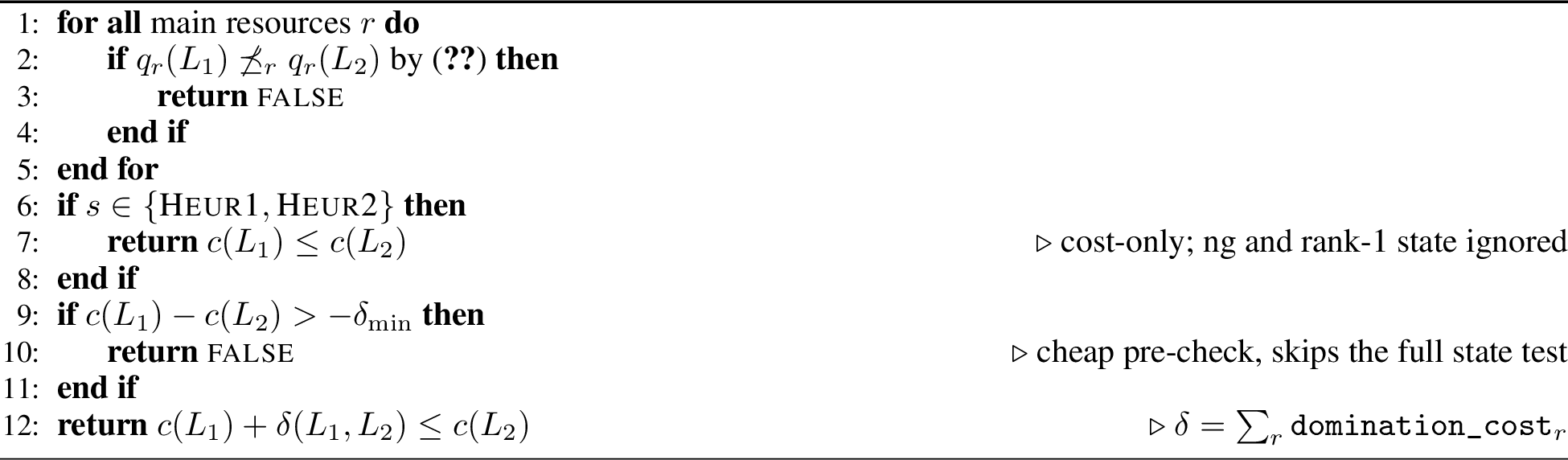
The algorithm builds partial paths as labels. A label \[\begin{align} L = \big(v(L),\; c(L),\; q(L),\; \pi(L)\big) \label{eq:label} \end{align}\tag{2}\] records its endpoint \(v(L)\), accumulated reduced cost \(c(L)\), the vector \(q(L)\in\mathbb{R}^{m}\) of the \(m\le 2\) main-resource values, and a tuple \(\pi(L)\) of the remaining per-resource states (the ng memory and rank-1 bits). A label is extended first along an arc and then on arrival at the new vertex by the REF 1 , the extensions of the individual resources composing into that of \(L\). The algorithm discards a label \(L_2\) when another label \(L_1\) at the same vertex dominates it: \(L_1\) is no worse on every main resource, \[\begin{align} q_r(L_1) \preceq_r q_r(L_2)\;\text{ for all } r,\qquad {\preceq_r} = \begin{cases} \le & r \text{ disposable, forward,}\\ \ge & r \text{ disposable, backward,}\\ = & r \text{ non-disposable,} \end{cases} \label{eq:order} \end{align}\tag{3}\] and cheap enough after a resource-dependent penalty, \[\begin{align} c(L_1) + \delta(L_1,L_2) \le c(L_2), \label{eq:dominance} \end{align}\tag{4}\] where \(\delta\) is a resource-dependent penalty charged when \(L_1\) is worse than \(L_2\) on some dimension. Each resource also exposes a constant \(\delta_{\min}\) (\(0\) for every resource shipped here) that drives a cheap pre-check: if \(c(L_1)-c(L_2) > -\delta_{\min}\) the full dominance test is skipped, which only ever retains a label and so is always safe. For an ordinary disposable resource \(\delta\in\{0,+\infty\}\); the rank-1 cut resource instead makes \(\delta\) finite, so a cheaper label can fail to dominate a dearer one; we return to this case in 3.5.
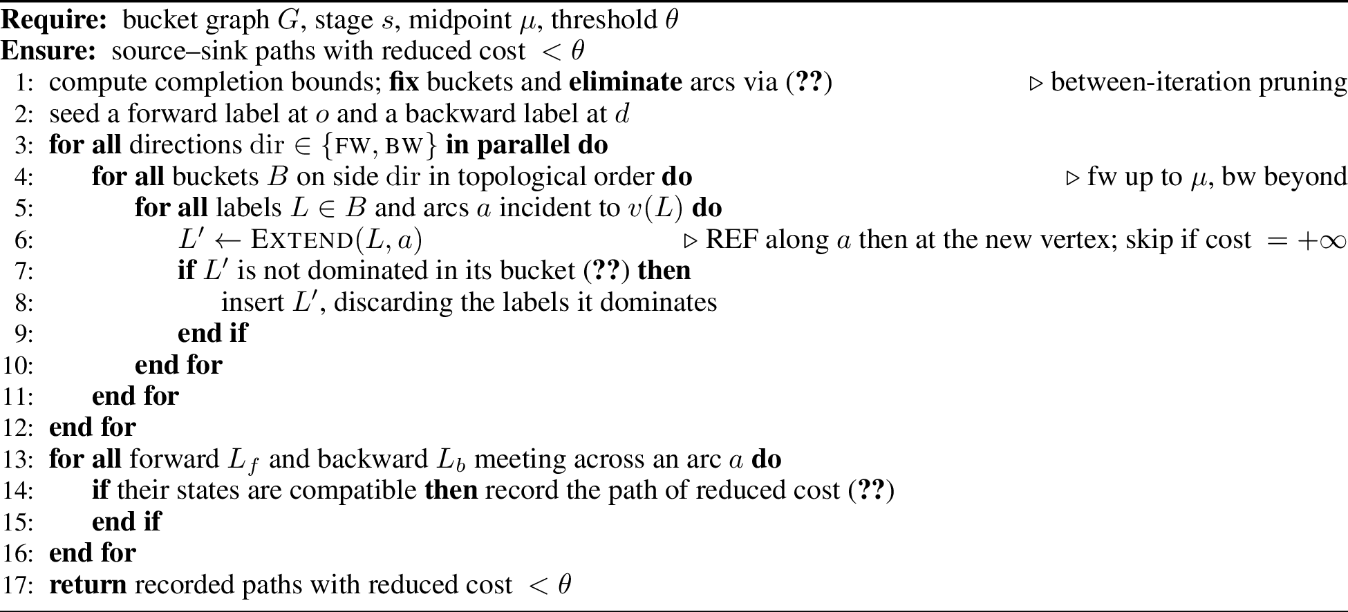
The bucket-graph algorithm [1] accelerates the search by partitioning the labels at each vertex into buckets indexed by their main-resource values (a one- or two-dimensional grid) and processing buckets in a topological order. A completion bound \(\underline{c}(B)\) (a lower bound on the cost-to-go from bucket \(B\) to the terminal) lets the algorithm prune: once a pricing threshold \(\theta\) is known, a bucket \(B\) with best-label cost \(c^\star(B)\) is fixed when \[\begin{align} c^\star(B) + \underline{c}(B) \ge \theta, \label{eq:fixing} \end{align}\tag{5}\] since none of its labels can then extend to an improving (\(<\theta\)) path, and arcs that likewise cannot lie on any improving path are eliminated, shrinking the graph between column-generation iterations. The search runs bidirectionally [9], extending forward labels to a midpoint \(\mu\) on the first main resource and backward labels beyond it, and recovers full paths by joining a forward label \(L_f\) and a backward label \(L_b\) across an arc [10] \(a=(i,j)\); the join is feasible when their states are compatible and yields reduced cost \[\begin{align} c(L_f) + c_a + c(L_b) + \gamma(L_f,L_b), \label{eq:concat} \end{align}\tag{6}\] with \(\gamma\) a resource-dependent concatenation term. 1 states the per-call labelling loop as the library implements it, and 2 the resource-generic dominance test it calls. What matters for the library is that the resource-dependent quantities they invoke (the REF 1 , the dominance penalty \(\delta\) and its lower bound \(\delta_{\min}\), and the concatenation term \(\gamma\)) are exactly the operations factored behind its resource interface (3).
3 Library design↩︎
The engine of 2 is generic over the resources a problem carries. Rather than fix a set of resources or dispatch on a runtime type, bgspprc expresses “a resource” as a C++23 concept and composes
resources at compile time. This section presents that interface (3.1), how resources compose (3.2) and how a problem is solved (3.3), the built-in resources
(3.4) including the rank-1 cut resource whose dual prices bend the usual dominance rule (3.5), the multi-stage solve (3.6), and the engineering choices
that set the library apart from PathWyse (3.7).
3.1 The resource concept↩︎
A resource is any type that supplies a state and the seven operations the labelling engine needs. The concept makes this requirement explicit and checkable at compile time ([lst:concept]). Each extension returns a pair (new_state, extra_cost); an extra_cost of \(+\infty\) signals infeasibility, so feasibility and cost flow through one
return value.
Listing lst:concept: The \texttt{Resource} concept (\texttt{include/bgspprc/resource.h}).
template <typename R>
concept Resource = requires(const R& r, Direction dir, Symmetry sym,
                            typename R::State s, typename R::State s2,
                            int arc_id, int vertex) {
  typename R::State;                                          // per-label state
  { r.symmetric() }            -> std::same_as<bool>;         // symmetric labeling?
  { r.init_state(dir) }        -> std::same_as<typename R::State>;
  { r.extend_along_arc(dir, s, arc_id) }                      // REF along an arc
                               -> std::same_as<std::pair<typename R::State, double>>;
  { r.extend_to_vertex(dir, s, vertex) }                      // REF at a vertex
                               -> std::same_as<std::pair<typename R::State, double>>;
  { r.domination_cost(dir, vertex, s, s2) } -> std::same_as<double>;   // delta in (2)
  { r.concatenation_cost(sym, vertex, s, s2) } -> std::same_as<double>;// fw/bw join
  { r.min_domination_cost() } -> std::same_as<double>;        // delta_min pre-check
};
The split between extend_along_arc and extend_to_vertex is deliberate: it separates the change a resource undergoes while traversing an arc from the change it undergoes on arriving at a vertex. For the ng-path resource
this is what keeps across-arc concatenation correct: the remembered set is remapped along the arc, but the arrival vertex is marked only at extend_to_vertex, so a label joined mid-arc is not charged twice for its endpoint. The
domination_cost function supplies the penalty \(\delta\) of 4 , concatenation_cost the join term of 2.2, and
min_domination_cost the constant \(\delta_{\min}\) used for the dominance pre-check.
3.2 Composing resources↩︎
A problem’s resources are bundled into a ResourcePack<Rs...>, a variadic template that holds the resource objects and presents the same seven operations to the engine. Every operation fans out over the pack with a fold expression over
std::index_sequence: extensions accumulate the cost and short-circuit to \(+\infty\) if any resource is infeasible, while the domination and pre-check costs are summed. Because the pack is a compile-time tuple,
the label state is std::tuple<typename Rs::State...>, its size is known at compile time, and no virtual dispatch occurs on the hot path. The empty pack ResourcePack<> is the no-extra-resource case (a plain
resource-constrained shortest path on the main resources alone).
Adding a new SPPRC variant therefore means writing one type that satisfies [lst:concept] and naming it in a pack. [lst:custom] shows a complete capacity resource that tracks accumulated arc demand: forward labels accumulate demand and become infeasible once it exceeds the vehicle capacity \(Q\), while
backward labels carry the remaining capacity and fail if it drops below zero, the two directions the bidirectional search of 2.2 requires. Because the resource is not symmetric (symmetric() returns
false), forward and backward states have different meanings, and the extension, dominance, and concatenation functions each branch on the direction.
Listing lst:custom: A complete user-defined resource (\texttt{examples/custom\_resource.cpp}, abridged).
struct CapacityResource {
  using State = double;                       // fw: demand used; bw: capacity left
  const double* demand;                       // per-arc demand
  double capacity;                            // Q
  bool symmetric() const { return false; }
  State init_state(Direction dir) const {
    return dir == Direction::Forward ? 0.0 : capacity;
  }
  std::pair<State,double> extend_along_arc(Direction dir, State s, int a) const {
    return {dir == Direction::Forward ? s + demand[a] : s - demand[a], 0.0};
  }
  std::pair<State,double> extend_to_vertex(Direction dir, State s, int) const {
    bool bad = dir == Direction::Forward ? s > capacity + EPS : s < -EPS;
    return {s, bad ? INF : 0.0};              // INF == infeasible
  }
  double domination_cost(Direction dir, int, State s1, State s2) const {
    bool worse = dir == Direction::Forward ? s1 > s2 + EPS : s1 < s2 - EPS;
    return worse ? INF : 0.0;                 // a worse state cannot dominate
  }
  double concatenation_cost(Symmetry, int, State s_fw, State s_bw) const {
    return s_fw + (capacity - s_bw) > capacity + EPS ? INF : 0.0;
  }
  double min_domination_cost() const { return 0.0; }
};
static_assert(bgspprc::Resource<CapacityResource>);          // checked at compile time
using Pack = bgspprc::ResourcePack<CapacityResource>;
3.3 Solving a problem↩︎
The graph is passed to the solver as a non-owning ProblemView: arrays of arc endpoints, costs, per-resource consumptions, and per-vertex windows that the caller continues to own. A solver is then instantiated on a pack and queried for
negative-cost paths. [lst:usage] shows the whole flow for a plain resource-constrained shortest path (the empty pack); swapping EmptyPack for the Pack
of [lst:custom] adds the capacity constraint with no other change. The pricing threshold \(\theta\) selects which paths are returned: a small
negative value keeps only improving columns for column generation, while a large value enumerates all feasible paths.
Listing lst:usage: Solving an SPPRC instance (adapted from \texttt{examples/basic\_spprc.cpp}).
using namespace bgspprc;
ProblemView pv;                                  // non-owning view of caller data
pv.n_vertices = n;  pv.source = 0;  pv.sink = n - 1;
pv.n_arcs = m;      pv.arc_from = from;  pv.arc_to = to;  pv.arc_base_cost = cost;
pv.n_resources = 1; pv.arc_resource = arc_res;             // one resource: time
pv.vertex_lb = v_lb; pv.vertex_ub = v_ub;  pv.n_main_resources = 1;

Solver<EmptyPack> solver(pv, EmptyPack{},
                         {.bucket_steps = {5.0, 1.0}, .theta = -1e-6});  // pricing
solver.set_stage(Stage::Exact);
solver.build();
for (const auto& p : solver.solve())             // paths with reduced cost < theta
  std::printf("cost=
3.4 Built-in resources↩︎
Five resources ship with the library, covering the variants of [10] (1). The
standard resource models time windows and capacity; when it is a main resource the bucket grid handles its extension directly for speed, and it is otherwise a pack member. The ng-path resource implements the elementarity relaxation of 2.1 with a compact local bit representation and the destination-marking split described above. The rank-1 cut resource carries up to 64 limited-memory rank-1 cuts in a bitset; it is the most instructive of the five
because its dual prices give it a dominance rule unlike any ordinary resource, and we treat it separately in 3.5. The cumulative-cost and pickup-and-delivery resources cover the cumulative-cost VRP and
simultaneous pickup-and-delivery, the former exercising genuinely non-zero arc cost deltas through extend_along_arc.
| Resource | State | Variant / role |
|---|---|---|
| Standard | double | time windows, capacity |
| Ng-path | uint32_t | elementarity relaxation |
| Rank-1 cuts | uint64_t | limited-memory rank-1 cuts |
| Cumulative cost | two doubles | cumulative-cost VRP |
| Pickup-delivery | two doubles | simultaneous pickup-and-delivery |
3.5 Rank-1 cuts: a resource that bends dominance↩︎
Subset-row cuts, introduced by Jepsen et al. [15] and generalized to the limited-memory rank-1 cuts [16] now central to modern branch-cut-and-price for routing [4], are a stringent test of whether an interface is really general, because their dominance does not fit the usual mould. A rank-1 cut places a coefficient on routes according to how often they visit a base set \(C\subseteq V\); the separated cut has dual price \(\sigma\le 0\), so completing a unit of the cut’s coefficient adds a reduced-cost penalty \(\beta=-\sigma\ge 0\) to a route: a label that has accumulated more coefficient is, all else equal, worse. What is unusual is that under limited memory a partially accumulated coefficient may be forgotten before it completes (below), so a label that is ahead on a cut is not infeasible, only at risk of a future \(+\beta\). The dominance penalty is therefore finite and positive rather than \(\{0,+\infty\}\): a label worse on its cut state can still dominate if it is cheap enough, and a cheaper label can fail to dominate, neither of which arises for an ordinary disposable resource.
The library expresses each cut as a single bit of a uint64_t state (up to 64 active cuts), specialized to the original three-row, \(p=\tfrac12\) subset-row cut. The two extension functions carry the
limited-memory bookkeeping. extend_along_arc applies the memory: it ANDs the state with a per-arc keep mask, clearing the bits of any cut whose memory does not contain the arc, so a route that strays outside a cut’s memory forgets its
partial accumulation. extend_to_vertex toggles the bits of every cut whose base set contains the vertex; a bit flipping from set to clear is an overflow (a full coefficient completed) and is charged \(+\beta\ge
0\), i.e.a penalty ([lst:r1c]).
Listing lst:r1c: The rank-1 cut extension functions (\texttt{include/bgspprc/r1c.h}, abridged).
std::pair<State,double> extend_along_arc(Direction, State s, int arc) const {
  return {s & arc_keep_mask_[arc], 0.0};        // limited memory: forget outside AM
}
std::pair<State,double> extend_to_vertex(Direction, State s, int v) const {
  uint64_t toggle = vertex_toggle_mask_[v];
  uint64_t overflow = s & toggle;               // bits that flip 1 -> 0
  return {s ^ toggle, overflow ? compute_overflow_cost(overflow) : 0.0};  // penalty >= 0
}
This contribution flows through the interface without special-casing the engine. Holding a cut bit is a disadvantage: the label is one base-set visit from completing a pair and paying the \(+\beta\) penalty, so
dominance must account for a penalty the dominator will face but the dominated label will not. If \(L_1\) holds a cut bit that \(L_2\) lacks, then on some completion \(L_1\) incurs a \(+\beta\) penalty that \(L_2\) escapes, so \(L_1\) must be correspondingly cheaper to dominate: the penalty
\(\delta\) of 4 is \(\sum_{\ell:\,b_\ell(L_1)\wedge\neg b_\ell(L_2)}\beta_\ell\ge 0\), one \(\beta_\ell\) per such cut, which
domination_cost returns. Unlike an ordinary disposable resource, whose penalty is \(0\) or \(+\infty\), the rank-1 resource thus contributes a finite, strictly positive
\(\delta\): a cheaper label can fail to dominate, and a label worse on its cut state can still dominate if it is cheap enough. The penalty is never negative (it is zero when \(L_1\) carries
no pending cut bit that \(L_2\) lacks), so min_domination_cost returns \(0\) and the pre-check of 2.2 needs no change. Concatenation is
symmetric: when a forward and a backward label share a cut bit, joining them completes that coefficient, so the join is charged the same \(+\beta\) overflow penalty. Nothing in the bucket-graph engine knows about cuts; the
resource supplies seven functions and the rest follows.
3.6 Multi-stage solve↩︎
A full exact labelling is wasteful while many negative-cost columns are easy to find, so the solver escalates automatically through three stages of increasing strength. Heuristic 1 keeps only the single cheapest label per bucket (the most aggressive pruning) and ignores the ng and rank-1 state; Heuristic 2 applies full bucket dominance but still ignores ng and rank-1; Exact runs the complete dominance of 4 over every resource. (The main-resource comparison is always enforced; the stages differ in how much of the remaining state they consult.) The solver advances when the current stage finds no improving columns (or after a few iterations), so the cheap stages carry the early column-generation iterations and the exact engine is reserved for the tail. Because a heuristic stage only prunes more aggressively, it can miss improving columns but never wrongly certify that none exist; the exact stage of 4 is therefore always run before the solver concludes that no negative-reduced-cost column remains, so the column-generation loop retains its optimality guarantee. Any column a heuristic stage does return is a genuine negative-reduced-cost path and may enter the restricted master directly. A separate Enumerate mode, invoked explicitly rather than as a rung of this ladder, disables dominance and enumerates all paths within the optimality gap up to a label budget, as required by some rank-1 cut separation routines.
3.7 Engineering and contrast with PathWyse↩︎
The library is header-only and depends only on the C++ standard library; a problem is solved by instantiating Solver<Pack, Executor> on a non-owning view of the graph data. Three engineering choices matter for performance. First,
labels are stored structure-of-arrays: costs, main resources, and ng/rank-1 bitsets live in parallel per-bucket arrays, so a dominance scan reads contiguous memory with no gather. Second, dominance is SIMD-accelerated over those arrays
(the cost and main-resource pre-filter vectorizes over double, and the ng subset tests over 32-bit lanes), using the <experimental/simd> parallelism TS where available, with a scalar fallback (its benefit is
instance-dependent; see 4.2). Third, parallelism is delegated to a pluggable Executor concept: the default executor is sequential, while a thread-pool executor (supplied as the Executor
template argument) runs forward and backward labelling concurrently and chunks the across-arc join with per-chunk buffers to avoid false sharing.
These choices distinguish bgspprc from PathWyse [2], the closest open comparator. PathWyse implements standard
labelling with decremental state-space relaxation and adds resources at runtime by subclassing a resource class; bgspprc implements the bucket-graph algorithm with bidirectional across-arc concatenation, bucket fixing, and arc elimination, and
composes resources at compile time with no dispatch on the hot path. The next section quantifies what this buys.
4 Computational study↩︎
We evaluate bgspprc on three public instance families. spprclib (45 instances) and roberti (31 instances) are capacity-constrained shortest-path pricing subproblems that arise in VRP column generation, taken from the
cptp repository and used in the capacitated-profitable-tour study of Jepsen et al. [17]: spprclib comprises the elementary
shortest-path-with-capacity instances of Jepsen, Petersen and Spoorendonk [18], and roberti was generated for that study by R. Roberti using
his pricing code from Baldacci, Mingozzi and Roberti [8]. rcspp is a standalone resource-constrained shortest-path benchmark generated
as VRPTW column-generation pricing subproblems from the 56 Solomon instances [19] and distributed as the rcspp_dataset collection [20]. Each instance is solved at ng-neighbourhood sizes \(n_g\in\{8,16,24\}\) with a 120 s timeout.
Instances are fetched from pinned public sources and the reference optima are committed; the bgspprc and PathWyse results are reproducible end to end (rebuild and re-run), and every table and figure regenerates from the committed result files
by a single command.
We report the shifted geometric mean (SGM) of runtimes, \(\exp\!\big(\overline{\log(t+s)}\big)-s\) with shift \(s=1\) s, alongside the arithmetic mean and the number of instances
solved within the timeout; timeouts are substituted at 120 s in both means rather than dropped, a conservative choice that never rewards a solver for failing. The 1 s shift keeps resolution in the sub-second regime where many instances sit. All runs were
performed on a single workstation with an AMD Ryzen 9 3950X processor (16 cores, 32 threads) and 128 GB of RAM, running Ubuntu 24.04 (Linux kernel 6.17). The library was built with GCC 14 and -march=native and run in its default SIMD-enabled
para_bidir mode at the hardware-default thread count (32 threads); PathWyse was built from a pinned upstream commit with the parity patches of 4.1 applied automatically. We do not profile memory or
per-component time; the focus is end-to-end pricing runtime. Every table and figure below is regenerated by a single command from the committed result files.
4.1 Comparison with PathWyse↩︎
PathWyse and bgspprc solve the same relaxation but tighten it differently by default, so a like-for-like runtime comparison requires that both compute the same bound. We therefore run both in pure-ng mode: two small
patches to PathWyse (both committed with the benchmark) align its ng-set construction with ours and remove its hard-coded two-cycle elimination, which is an extra tightening the pure ng-relaxation does not include. With these, every instance on which both
solvers finish agrees on the optimal reduced cost up to cost-scale rounding, so 2 compares runtime at a fixed bound.
| Set | \(n_g\) | bgspprc | PathWyse | Speedup | ||||||
|---|---|---|---|---|---|---|---|---|---|---|
| sgm | mean | solved | \(\text{sgm}_1\) | sgm | mean | solved | 32-thr | 1-thr | ||
| spprclib | 8 | 0.917 | 7.238 | 44/45 | 0.922 | 1.522 | 12.133 | 42/45 | 1.32\(\times\) | 1.31\(\times\) |
| spprclib | 16 | 2.048 | 15.801 | 40/45 | 1.997 | 4.284 | 24.290 | 38/45 | 1.73\(\times\) | 1.76\(\times\) |
| spprclib | 24 | 5.838 | 26.725 | 38/45 | 5.286 | 10.590 | 42.512 | 31/45 | 1.69\(\times\) | 1.84\(\times\) |
| roberti | 8 | 0.551 | 0.911 | 31/31 | 0.636 | 2.330 | 9.999 | 30/31 | 2.15\(\times\) | 2.03\(\times\) |
| roberti | 16 | 3.176 | 15.003 | 28/31 | 3.239 | 8.796 | 28.152 | 28/31 | 2.35\(\times\) | 2.31\(\times\) |
| roberti | 24 | 14.813 | 44.346 | 23/31 | 14.247 | 26.824 | 62.019 | 19/31 | 1.76\(\times\) | 1.82\(\times\) |
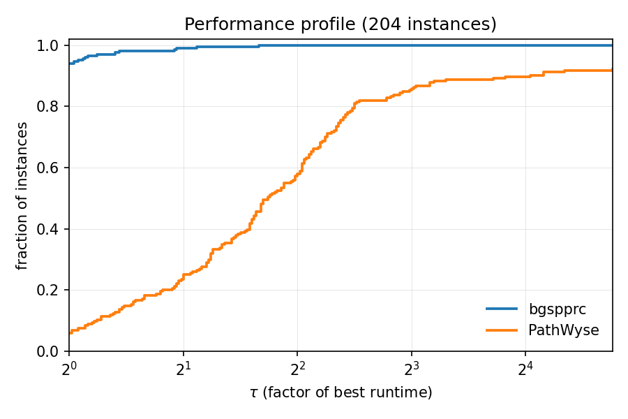
Across all six (set, \(n_g\)) cells, bgspprc is faster than PathWyse by shifted geometric mean, with per-cell speedups of \(1.3\times\)–\(2.35\times\) (2); it also solves at least as many instances within the timeout in every cell, and strictly more in five of the six (tying only on roberti at \(n_g=16\)). The advantage is largest on the roberti instances at \(n_g=8\) and \(n_g=16\) (\(2.15\times\) and \(2.35\times\)). The performance profile (3) shows the same conclusion instance by instance: bgspprc is the faster solver on the large majority of instances and its curve dominates
PathWyse’s throughout. Since both solvers compute the same bound, this is a runtime advantage at equal strength, which we attribute to the bucket-graph pruning and the structure-of-arrays label store of 3.7.
Two further observations support reading these numbers as a genuine result at equal bound. First, on correctness: of the 228 (instance, \(n_g\)) pairs, both solvers finish within the timeout on 188. On 152 of those the
optimal reduced cost is bit-identical and on 185 the two agree to within \(0.002\), a rounding artifact of PathWyse’s integer cost scaling. Of the three pairs that differ by more, bgspprc reports a strictly
better bound on two (by up to \(0.137\)) and a bound worse by only \(0.002\) (itself at the rounding tolerance) on the third; bgspprc’s optimum is thus never more than
\(0.002\) worse than PathWyse’s, confirming that the parity construction yields the same LP bound and that our implementation is correct against an independent reference. Second, on the head-to-head: among the 188 jointly
solved pairs bgspprc is strictly faster on 176 and slower on only 12, so the SGM advantage is not an artifact of a few large instances but holds broadly across the benchmark.
A note on compute. 2 reports each solver in its default configuration: bgspprc’s para_bidir mode runs forward and backward labelling concurrently (32 threads here), whereas PathWyse is
single-threaded by design. We compare the two libraries as each is intended to be run; exploiting parallelism is part of the implementation, not a thumb on the scale. That the advantage is nonetheless algorithmic rather than a parallelism artifact
is shown by the \(\text{sgm}_1\) and 1-thr columns of 2, which repeat the comparison with bgspprc restricted to a single thread (its sequential bidir_base build):
even then it is \(1.3\times\)–\(2.3\times\) faster than PathWyse at the identical bound in every cell and solves at least as many instances. At the largest neighbourhoods (\(n_g=24\)) the single-threaded build is in fact faster than the parallel one, whose thread-pool overhead does not pay off there. We therefore attribute the advantage primarily to the bucket-graph pruning and the
structure-of-arrays label store of 3.7, with thread-level parallelism adding a further margin on top.
The gap between the SGM and the arithmetic mean in 2 (the arithmetic mean is several times larger for both solvers) reflects a heavy tail of hard instances near the timeout that both solvers share.
4.2 Mode and SIMD ablation↩︎
To see where the runtime goes, 3 ablates the two execution axes on the rcspp set: monodirectional versus bidirectional versus parallel-bidirectional search, each with SIMD on or off. Two patterns stand out.
Monodirectional search is fastest at \(n_g=8\), where the search trees are shallow and the bookkeeping of splitting into forward and backward halves does not pay off; from \(n_g=16\) upward
the parallel-bidirectional mode catches up and stays within a sub-second SGM of the leader. The one outlier is para_bidir_base at \(n_g=8\) (SGM 8.80 s, 37/56 solved), a real cliff for the scalar
parallel-bidirectional mode on the shallowest setting that the SIMD default (para_bidir_vec, 1.88 s, 56/56) avoids.
The SIMD axis deserves comment, because vectorizing the dominance check does not help here: for the mono and bidir modes _vec and _base differ by under 5% on rcspp (the para_bidir_base cliff at \(n_g=8\) aside), and on the larger spprclib and roberti instances (6) the vectorized build is frequently slower, by up to about \(40\%\). This
follows from how the two scan a bucket. The scalar check exploits the cost-sorted label store: it begins at the first label that could be dominated and stops at the first dominator, so it usually settles a label after a handful of comparisons. By contrast,
the vectorized check evaluates a fixed-width batch of candidates against each stored label before it can stop. The batch only amortizes its overhead when many labels per bucket survive the cost and main-resource pre-filter and must be compared in full; on
these pure-ng instances, with one or two main resources and cost-sorted buckets, that surviving set is small and the scalar early-exit wins. We therefore conjecture that SIMD dominance pays off precisely when this early termination is defeated:
when the non-dominated frontier per bucket is wide and the cost pre-filter is weak. The clearest such regime is pricing with active limited-memory rank-1 cuts (3.5): there a cut’s dominance penalty \(\delta\) is finite and positive rather than \(\{0,+\infty\}\), so a cheaper label can fail to dominate while a label worse on its cut state can still dominate. Both effects defeat the
cost-sorted early-exit and enlarge the set of mutually non-dominated labels, exactly the conditions the vectorized scan is built for. Our benchmark runs pure ng with no cuts, the regime in which SIMD has least to do; evaluating it under rank-1-cut and
higher-dimensional resource pricing is left as future work. One consequence is that the headline comparison is conservative: it reports the SIMD default (para_bidir_vec) throughout, even though the scalar configurations are often
faster still.
4 distils the six modes into one SGM speedup ratio per execution axis, each isolated on the scalar, single-thread, bidirectional baseline, and confirms three patterns. Direction is the dominant axis and
changes sign with search depth: monodirectional search is faster on the shallow rcspp instances and on spprclib at \(n_g=8\) (\(0.4\)–\(0.6\times\)), while
bidirectional search is up to \(3.1\times\) faster once the search deepens (spprclib \(n_g\ge16\), roberti throughout). Threads add a smaller, near-constant \(1.02\)–\(1.27\times\) on top of bidirectional search everywhere except the scalar rcspp \(n_g=8\) cliff. SIMD never helps on these pure-ng instances
(\(0.74\)–\(0.99\times\)); its only role is to rescue that cliff. The fastest build in all but one cell is therefore a scalar one (monodirectional when the search is shallow, scalar
parallel-bidirectional when it is deep; the lone exception is rcspp \(n_g=8\), where vectorized monodirectional labelling wins by a negligible margin), yet each of those has a regime in which it collapses:
para_bidir_base times out on 19 of the 56 easiest rcspp \(n_g=8\) instances, and mono is roughly \(3\times\) slower and solves fewer of the deep roberti instances.
The shipped default para_bidir_vec is never the per-cell fastest, but it is the only build with no catastrophic regime, robust rather than universally optimal. A search-depth-adaptive policy that selects monodirectional labelling for the
smallest subproblems and parallel-bidirectional labelling otherwise would capture the per-cell best of both; we leave it to future work.
| \(n_g\) | mode | sgm (s) | mean (s) | solved |
|---|---|---|---|---|
| 8 | mono_base | 1.296 | 2.885 | 56/56 |
| mono_vec | 1.288 | 2.850 | 56/56 | |
| bidir_base | 2.389 | 7.870 | 56/56 | |
| bidir_vec | 2.442 | 7.995 | 56/56 | |
| para_bidir_base | 8.798 | 44.624 | 37/56 | |
| para_bidir_vec | 1.884 | 5.640 | 56/56 | |
| 16 | mono_base | 1.578 | 4.979 | 56/56 |
| mono_vec | 1.598 | 5.134 | 56/56 | |
| bidir_base | 2.824 | 12.800 | 55/56 | |
| bidir_vec | 2.855 | 12.952 | 55/56 | |
| para_bidir_base | 2.222 | 8.913 | 56/56 | |
| para_bidir_vec | 2.200 | 8.783 | 56/56 | |
| 24 | mono_base | 1.940 | 11.005 | 54/56 |
| mono_vec | 1.974 | 11.567 | 54/56 | |
| bidir_base | 3.156 | 17.821 | 51/56 | |
| bidir_vec | 3.222 | 18.443 | 51/56 | |
| para_bidir_base | 2.532 | 14.792 | 52/56 | |
| para_bidir_vec | 2.588 | 15.433 | 52/56 |
| set | \(n_g\) | Direction | Threads | SIMD | fastest |
|---|---|---|---|---|---|
| mono\(\to\)bidir | bidir\(\to\)para | base\(\to\)vec | mode | ||
| rcspp | 8 | 0.54\(\times\) | 0.27\(\times\) | 0.98\(\times\) | mono_vec |
| 16 | 0.56\(\times\) | 1.27\(\times\) | 0.99\(\times\) | mono_base | |
| 24 | 0.61\(\times\) | 1.25\(\times\) | 0.98\(\times\) | mono_base | |
| spprclib | 8 | 0.42\(\times\) | 1.02\(\times\) | 0.98\(\times\) | mono_base |
| 16 | 1.18\(\times\) | 1.06\(\times\) | 0.90\(\times\) | para_bidir_base | |
| 24 | 3.09\(\times\) | 1.09\(\times\) | 0.81\(\times\) | para_bidir_base | |
| roberti | 8 | 1.38\(\times\) | 1.25\(\times\) | 0.91\(\times\) | para_bidir_base |
| 16 | 2.39\(\times\) | 1.22\(\times\) | 0.81\(\times\) | para_bidir_base | |
| 24 | 3.08\(\times\) | 1.26\(\times\) | 0.74\(\times\) | para_bidir_base |
4.3 Context: comparison with parallel pull labelling↩︎
Finally, we place bgspprc against the parallel pull-labelling algorithm of Petersen and Spoorendonk [3],
as implemented in the Flowty solver [21], on the rcspp set (5). The pull-labelling runtimes are those reported in that paper on
the same instances (committed as pull_algo_runtimes.csv). Pull labelling is a different, independently developed labelling technique for the same problem (in principle equally general) rather than a specialized single-purpose solver; the two
are distinct points in the algorithmic design space. bgspprc runs within \(1.9\times\)–\(2.4\times\) of it in SGM on the same instances (\(n_g\in\{8,16\}\); one fewer at \(n_g=24\), 52 versus 53 of 56), and the gap narrows monotonically as \(n_g\) grows (\(2.40\times \to
2.10\times \to 1.92\times\)), suggesting a fixed per-instance overhead rather than one that scales with the search. The comparison is best read as locating bgspprc against a strong, independent alternative on shared instances rather
than as a generality-versus-specialization trade-off; that bgspprc stays within a small constant factor while adding compile-time extensibility and built-in cut support is the takeaway. We do not measure how the two methods compare across
graph densities (a pull step that gathers each label from its predecessors has less to amortize on the sparse pricing graphs used here than on dense ones), but this is conjecture, and a characterization across densities is left to future work.
| \(n_g\) | bgspprc | pull-labelling | Slowdown | ||||
|---|---|---|---|---|---|---|---|
| sgm | mean | solved | sgm | mean | solved | ||
| 8 | 1.884 | 5.640 | 56/56 | 0.203 | 0.406 | 56/56 | 2.40\(\times\) |
| 16 | 2.200 | 8.783 | 56/56 | 0.526 | 3.010 | 56/56 | 2.10\(\times\) |
| 24 | 2.588 | 15.433 | 52/56 | 0.873 | 9.123 | 53/56 | 1.92\(\times\) |
5 Conclusions↩︎
We have presented bucket-graph-spprc, an open-source, header-only C++23 library for the SPPRC. It implements the bucket-graph labelling algorithm with bidirectional across-arc concatenation, bucket fixing, and arc elimination, and is
organized around a compile-time resource concept that lets a new SPPRC variant be added by implementing a fixed seven-function interface, with resources composed into the label state with no runtime dispatch. On shared public instances, at an equal LP
bound, bgspprc is \(1.3\times\)–\(2.35\times\) faster than PathWyse, the main open-source comparator, and runs within \(1.9\times\)–\(2.4\times\) of parallel pull labelling, a different labelling technique for the same problem, while remaining general and extensible. The library, the benchmark scripts, and the pinned instances are publicly available under a
permissive licence, and every table and figure in this paper is reproduced by a single command.
The algorithms are not new; the contribution is an open, performant, and extensible implementation, together with a reproducible benchmark, of methods that were previously available only in academic or closed solvers. Several directions remain. The resource interface invites further built-in resources beyond the five shipped here; integrating the pricer into a full branch-cut-and-price loop would exercise it under repeated re-solves with cuts and branching; and the gap to parallel pull labelling, which our ablation suggests is a fixed per-instance overhead, is worth closing. The library is intended to lower the barrier to building on the bucket-graph algorithm.
Code and data availability↩︎
The bucket-graph-spprc library is open source under the MIT licence at https://github.com/spoorendonk/bucket-graph-spprc. Its benchmarks/ directory
contains the run and comparison scripts, the two PathWyse parity patches, the reference optima, and the committed result files from which every table and figure in this paper is regenerated by a single command. The instance sets are fetched from public
repositories: the spprclib and roberti pricing instances from https://github.com/spoorendonk/cptp and the Solomon RCSPP set from https://github.com/spoorendonk/rcspp_dataset. PathWyse is cloned from its upstream repository and built from a pinned commit with the two parity patches applied automatically. An archival snapshot of the library (v0.1.0) is deposited on
Zenodo [22]: the version DOI 10.5281/zenodo.20819209 pins the exact release this paper describes, while the concept DOI
10.5281/zenodo.20819208 always resolves to the latest version.
Disclosure statement↩︎
The author is affiliated with Flowty (https://flowty.ai), whose solver provides the parallel pull-labelling implementation [21] used as a comparator in 4.3. All benchmark scripts, instances, and reference results are public, so the comparison is independently reproducible.
6 Full mode and SIMD ablation↩︎
6 gives the mode and SIMD ablation of 4.2 across all three instance sets, complementing the rcspp slice in 3. The pattern is consistent with the
main text. On the smaller spprclib instances monodirectional search is fastest at \(n_g=8\), but the bidirectional modes overtake it from \(n_g=16\) onward as the search deepens. On roberti
the parallel-bidirectional mode is fastest at every \(n_g\), in its scalar form para_bidir_base throughout. Across both sets the _vec builds run slower than their _base counterparts,
by up to about \(40\%\) on the largest instances, so the fastest configuration is frequently a scalar one; 4.2 explains the mechanism and conjectures when vectorization would instead
pay off.
| set | \(n_g\) | mode | sgm (s) | mean (s) | solved |
|---|---|---|---|---|---|
| spprclib | 8 | mono_base | 0.390 | 3.026 | 44/45 |
| mono_vec | 0.429 | 3.094 | 44/45 | ||
| bidir_base | 0.922 | 7.170 | 44/45 | ||
| bidir_vec | 0.941 | 7.309 | 44/45 | ||
| para_bidir_base | 0.905 | 7.169 | 44/45 | ||
| para_bidir_vec | 0.917 | 7.238 | 44/45 | ||
| spprclib | 16 | mono_base | 2.354 | 7.058 | 44/45 |
| mono_vec | 3.336 | 9.628 | 44/45 | ||
| bidir_base | 1.997 | 15.773 | 40/45 | ||
| bidir_vec | 2.224 | 16.100 | 40/45 | ||
| para_bidir_base | 1.875 | 15.586 | 40/45 | ||
| para_bidir_vec | 2.048 | 15.801 | 40/45 | ||
| spprclib | 24 | mono_base | 16.323 | 46.133 | 34/45 |
| mono_vec | 22.270 | 55.078 | 30/45 | ||
| bidir_base | 5.286 | 25.308 | 38/45 | ||
| bidir_vec | 6.533 | 27.552 | 38/45 | ||
| para_bidir_base | 4.869 | 24.788 | 38/45 | ||
| para_bidir_vec | 5.838 | 26.725 | 38/45 | ||
| roberti | 8 | mono_base | 0.880 | 1.470 | 31/31 |
| mono_vec | 1.022 | 1.774 | 31/31 | ||
| bidir_base | 0.636 | 1.133 | 31/31 | ||
| bidir_vec | 0.697 | 1.246 | 31/31 | ||
| para_bidir_base | 0.511 | 0.851 | 31/31 | ||
| para_bidir_vec | 0.551 | 0.911 | 31/31 | ||
| roberti | 16 | mono_base | 7.750 | 28.426 | 27/31 |
| mono_vec | 10.484 | 32.769 | 25/31 | ||
| bidir_base | 3.239 | 15.128 | 28/31 | ||
| bidir_vec | 3.981 | 16.270 | 28/31 | ||
| para_bidir_base | 2.649 | 14.165 | 28/31 | ||
| para_bidir_vec | 3.176 | 15.003 | 28/31 | ||
| roberti | 24 | mono_base | 43.841 | 70.594 | 17/31 |
| mono_vec | 57.345 | 79.861 | 15/31 | ||
| bidir_base | 14.247 | 42.547 | 24/31 | ||
| bidir_vec | 19.242 | 48.893 | 23/31 | ||
| para_bidir_base | 11.300 | 38.679 | 25/31 | ||
| para_bidir_vec | 14.813 | 44.346 | 23/31 | ||
| rcspp | 8 | mono_base | 1.296 | 2.885 | 56/56 |
| mono_vec | 1.288 | 2.850 | 56/56 | ||
| bidir_base | 2.389 | 7.870 | 56/56 | ||
| bidir_vec | 2.442 | 7.995 | 56/56 | ||
| para_bidir_base | 8.798 | 44.624 | 37/56 | ||
| para_bidir_vec | 1.884 | 5.640 | 56/56 | ||
| rcspp | 16 | mono_base | 1.578 | 4.979 | 56/56 |
| mono_vec | 1.598 | 5.134 | 56/56 | ||
| bidir_base | 2.824 | 12.800 | 55/56 | ||
| bidir_vec | 2.855 | 12.952 | 55/56 | ||
| para_bidir_base | 2.222 | 8.913 | 56/56 | ||
| para_bidir_vec | 2.200 | 8.783 | 56/56 | ||
| rcspp | 24 | mono_base | 1.940 | 11.005 | 54/56 |
| mono_vec | 1.974 | 11.567 | 54/56 | ||
| bidir_base | 3.156 | 17.821 | 51/56 | ||
| bidir_vec | 3.222 | 18.443 | 51/56 | ||
| para_bidir_base | 2.532 | 14.792 | 52/56 | ||
| para_bidir_vec | 2.588 | 15.433 | 52/56 |
7 Per-instance results↩︎
For completeness and to back the aggregated cells of 2 and 5, this appendix lists every instance’s wall-clock time. 1 covers the spprclib and roberti sets (bgspprc para_bidir versus patched PathWyse, both pure-ng); 2 covers the rcspp set (bgspprc versus parallel pull labelling). Times are in seconds at each \(n_g\in\{8,16,24\}\), with t/o marking a 120 s timeout; the
shifted geometric mean of each solver column reproduces the corresponding cell of the in-text tables. These tables are regenerated from the committed result files by the same single command as the rest of the paper.
| Instance | \(n_g=8\) | \(n_g=16\) | \(n_g=24\) | |||
| bg | pw | bg | pw | bg | pw | |
| (1 continued) | ||||||
| Instance | \(n_g=8\) | \(n_g=16\) | \(n_g=24\) | |||
| bg | pw | bg | pw | bg | pw | |
| continued on next page | ||||||
| A-n54-k7-149 | 0.051 | 0.153 | 0.311 | 0.674 | 2.372 | 2.726 |
| A-n60-k9-57 | 0.063 | 0.147 | 0.338 | 0.528 | 1.705 | 1.464 |
| A-n61-k9-80 | 0.067 | 0.155 | 0.270 | 0.869 | 2.220 | 4.204 |
| A-n62-k8-99 | 0.114 | 0.533 | 0.915 | 3.342 | 8.839 | 32.199 |
| A-n63-k10-44 | 0.049 | 0.131 | 0.237 | 0.538 | 1.192 | 1.546 |
| A-n63-k9-157 | 0.048 | 0.152 | 0.196 | 0.582 | 0.884 | 1.751 |
| A-n64-k9-45 | 0.098 | 0.423 | 0.349 | 1.810 | 1.630 | 8.344 |
| A-n65-k9-10 | 0.083 | 0.196 | 0.367 | 0.975 | 2.030 | 3.544 |
| A-n69-k9-42 | 0.073 | 0.227 | 0.387 | 0.897 | 1.716 | 2.506 |
| A-n80-k10-14 | 0.771 | 2.043 | 5.698 | 17.017 | 23.151 | t/o |
| B-n45-k6-54 | 0.062 | 0.253 | 0.082 | 0.558 | 0.325 | 6.576 |
| B-n50-k8-40 | 0.044 | 0.169 | 0.427 | 1.329 | 4.526 | 7.872 |
| B-n52-k7-15 | 0.154 | 0.226 | 5.355 | 22.080 | 39.616 | t/o |
| B-n57-k7-20 | 0.537 | 4.895 | 0.613 | 5.465 | 0.652 | 10.659 |
| B-n66-k9-50 | 0.136 | 1.329 | 5.625 | 39.999 | 38.130 | t/o |
| B-n67-k10-26 | 0.093 | 0.371 | 0.948 | 1.836 | 9.566 | 9.693 |
| B-n68-k9-65 | 0.158 | 0.501 | 1.112 | 6.245 | 31.232 | t/o |
| B-n78-k10-70 | 0.171 | 0.507 | 1.432 | 5.158 | 103.154 | t/o |
| E-n101-k14-158 | 0.129 | 0.418 | 0.695 | 1.377 | 4.428 | 4.435 |
| E-n101-k8-291 | 0.194 | 0.993 | 1.312 | 5.261 | 11.985 | 22.989 |
| E-n76-k10-72 | 0.129 | 0.503 | 0.880 | 3.786 | 7.413 | 33.895 |
| E-n76-k14-102 | 0.064 | 0.089 | 0.179 | 0.241 | 0.679 | 0.648 |
| E-n76-k15-40 | 0.036 | 0.080 | 0.177 | 0.212 | 0.538 | 0.492 |
| E-n76-k7-44 | 0.214 | 0.660 | 1.633 | 5.286 | 17.856 | 60.875 |
| G-n262-k25-316 | t/o | t/o | t/o | t/o | t/o | t/o |
| M-n101-k10-97 | 0.365 | 2.097 | 2.194 | 28.595 | 33.746 | t/o |
| M-n121-k7-260 | 43.552 | t/o | t/o | t/o | t/o | t/o |
| M-n151-k12-15 | 27.692 | 31.453 | t/o | t/o | t/o | t/o |
| M-n200-k16-143 | 5.308 | 94.768 | 6.481 | t/o | 7.926 | t/o |
| M-n200-k17-12 | 65.031 | t/o | t/o | t/o | t/o | t/o |
| P-n101-k4-174 | 1.988 | 8.695 | 15.499 | t/o | t/o | t/o |
| P-n50-k10-24 | 0.014 | 0.019 | 0.027 | 0.039 | 0.041 | 0.056 |
| P-n50-k7-92 | 0.018 | 0.053 | 0.039 | 0.179 | 0.065 | 0.361 |
| P-n50-k8-19 | 0.052 | 0.114 | 0.096 | 0.178 | 0.183 | 0.512 |
| P-n51-k10-30 | 0.018 | 0.023 | 0.060 | 0.054 | 0.170 | 0.090 |
| P-n55-k10-44 | 0.016 | 0.033 | 0.037 | 0.089 | 0.063 | 0.169 |
| P-n55-k15-88 | 0.018 | 0.020 | 0.030 | 0.023 | 0.060 | 0.028 |
| P-n55-k7-116 | 0.037 | 0.123 | 0.144 | 0.595 | 0.475 | 1.945 |
| P-n55-k8-260 | 0.031 | 0.078 | 0.129 | 0.324 | 0.496 | 0.780 |
| P-n60-k10-24 | 0.035 | 0.080 | 0.114 | 0.272 | 0.480 | 0.901 |
| P-n60-k15-8 | 0.014 | 0.017 | 0.024 | 0.028 | 0.034 | 0.036 |
| P-n65-k10-102 | 0.023 | 0.063 | 0.058 | 0.196 | 0.140 | 0.548 |
| P-n70-k10-12 | 0.188 | 0.396 | 0.654 | 2.159 | 2.887 | 11.198 |
| P-n76-k4-41 | 46.847 | 24.615 | t/o | t/o | t/o | t/o |
| P-n76-k5-16 | 10.934 | 8.169 | 55.936 | 94.270 | t/o | t/o |
| roberti | ||||||
| E-n101-k14_a | 0.148 | 0.441 | 0.773 | 1.532 | 5.413 | 5.288 |
| E-n101-k14_b | 0.121 | 0.365 | 0.659 | 1.290 | 4.616 | 4.297 |
| E-n101-k8_a | 0.361 | 1.648 | 2.410 | 11.429 | 38.492 | 117.529 |
| E-n101-k8_b | 0.154 | 0.752 | 0.944 | 3.008 | 7.878 | 10.266 |
| E-n76-k10_a | 0.088 | 0.256 | 0.519 | 1.281 | 2.913 | 4.350 |
| E-n76-k10_b | 0.054 | 0.194 | 0.256 | 0.819 | 1.025 | 2.402 |
| E-n76-k14_a | 0.039 | 0.092 | 0.153 | 0.265 | 0.617 | 0.688 |
| E-n76-k14_b | 0.040 | 0.092 | 0.159 | 0.247 | 0.651 | 0.714 |
| E-n76-k7_a | 0.140 | 0.640 | 1.308 | 4.596 | 13.841 | 32.507 |
| E-n76-k7_b | 0.117 | 0.478 | 0.622 | 3.497 | 3.637 | 17.070 |
| E-n76-k8_a | 0.099 | 0.416 | 0.629 | 2.517 | 4.124 | 12.644 |
| E-n76-k8_b | 0.054 | 0.211 | 0.158 | 0.899 | 0.546 | 2.871 |
| F-n135-k7_a | 3.620 | 64.392 | t/o | t/o | t/o | t/o |
| F-n45-k4_a | 0.125 | 0.317 | 0.415 | 2.829 | 3.646 | 51.195 |
| F-n72-k4_a | 9.742 | 3.115 | 15.717 | 74.461 | 49.041 | t/o |
| M-n121-k7_a | 2.903 | t/o | t/o | t/o | t/o | t/o |
| M-n121-k7_b | 1.937 | 52.127 | t/o | t/o | t/o | t/o |
| M-n151-k12_a | 0.674 | 4.964 | 5.929 | 32.903 | 102.890 | t/o |
| M-n151-k12_b | 0.591 | 4.140 | 5.489 | 25.701 | 86.183 | t/o |
| M-n200-k16_a | 1.612 | 14.223 | 16.548 | 83.345 | t/o | t/o |
| M-n200-k16_b | 1.454 | 11.413 | 15.165 | 61.544 | t/o | t/o |
| M-n200-k17_a | 1.332 | 10.727 | 11.460 | 58.021 | t/o | t/o |
| M-n200-k17_b | 1.332 | 9.988 | 12.033 | 51.121 | t/o | t/o |
| P-n101-k4_a | 0.561 | 4.468 | 6.561 | 53.694 | t/o | t/o |
| P-n101-k4_b | 0.266 | 1.317 | 1.473 | 7.599 | 18.415 | 58.645 |
| P-n70-k10_a | 0.038 | 0.115 | 0.136 | 0.379 | 0.359 | 1.236 |
| P-n70-k10_b | 0.053 | 0.103 | 0.091 | 0.335 | 0.285 | 1.172 |
| P-n76-k4_a | 0.225 | 1.202 | 2.555 | 14.021 | 38.199 | t/o |
| P-n76-k4_b | 0.103 | 0.463 | 0.678 | 3.576 | 6.346 | 27.046 |
| P-n76-k5_a | 0.161 | 0.902 | 1.724 | 9.157 | 21.948 | 117.527 |
| P-n76-k5_b | 0.097 | 0.422 | 0.527 | 2.655 | 3.675 | 15.134 |
| Instance | \(n_g=8\) | \(n_g=16\) | \(n_g=24\) | |||
| bg | pull | bg | pull | bg | pull | |
| (2 continued) | ||||||
| Instance | \(n_g=8\) | \(n_g=16\) | \(n_g=24\) | |||
| bg | pull | bg | pull | bg | pull | |
| continued on next page | ||||||
| C101 | 0.029 | 0.010 | 0.029 | 0.010 | 0.030 | 0.010 |
| C102 | 0.205 | 0.017 | 0.218 | 0.016 | 0.211 | 0.017 |
| C103 | 0.423 | 0.023 | 0.431 | 0.026 | 0.452 | 0.030 |
| C104 | 0.761 | 0.057 | 0.894 | 0.319 | 0.812 | 0.121 |
| C105 | 0.060 | 0.009 | 0.067 | 0.009 | 0.070 | 0.009 |
| C106 | 0.099 | 0.010 | 0.083 | 0.010 | 0.082 | 0.010 |
| C107 | 0.113 | 0.009 | 0.125 | 0.009 | 0.123 | 0.010 |
| C108 | 0.146 | 0.013 | 0.139 | 0.012 | 0.138 | 0.013 |
| C109 | 0.254 | 0.017 | 0.240 | 0.017 | 0.256 | 0.017 |
| C201 | 0.242 | 0.010 | 0.282 | 0.010 | 0.269 | 0.010 |
| C202 | 6.180 | 0.030 | 6.264 | 0.040 | 6.884 | 0.084 |
| C203 | 17.696 | 0.163 | 20.527 | 2.478 | 18.696 | 0.571 |
| C204 | 32.341 | 2.961 | 38.406 | 16.294 | 94.144 | t/o |
| C205 | 0.613 | 0.020 | 0.600 | 0.020 | 0.593 | 0.017 |
| C206 | 1.077 | 0.037 | 1.057 | 0.033 | 1.105 | 0.030 |
| C207 | 1.736 | 0.211 | 1.729 | 0.277 | 1.634 | 0.095 |
| C208 | 1.510 | 0.044 | 1.516 | 0.040 | 1.557 | 0.041 |
| R101 | 0.015 | 0.006 | 0.014 | 0.006 | 0.013 | 0.006 |
| R102 | 0.107 | 0.011 | 0.108 | 0.012 | 0.084 | 0.012 |
| R103 | 0.201 | 0.019 | 0.207 | 0.019 | 0.217 | 0.018 |
| R104 | 0.514 | 0.038 | 0.662 | 0.063 | 0.664 | 0.056 |
| R105 | 0.046 | 0.008 | 0.042 | 0.008 | 0.053 | 0.008 |
| R106 | 0.171 | 0.017 | 0.150 | 0.017 | 0.166 | 0.018 |
| R107 | 0.346 | 0.037 | 0.354 | 0.042 | 0.358 | 0.038 |
| R108 | 0.656 | 0.063 | 0.715 | 0.073 | 0.778 | 0.081 |
| R109 | 0.117 | 0.013 | 0.137 | 0.013 | 0.120 | 0.013 |
| R110 | 0.252 | 0.020 | 0.267 | 0.020 | 0.255 | 0.020 |
| R111 | 0.310 | 0.037 | 0.338 | 0.041 | 0.342 | 0.042 |
| R112 | 0.581 | 0.047 | 0.610 | 0.062 | 0.600 | 0.063 |
| R201 | 0.738 | 0.016 | 0.769 | 0.017 | 0.724 | 0.017 |
| R202 | 5.760 | 0.084 | 5.695 | 0.101 | 5.931 | 0.139 |
| R203 | 18.320 | 0.293 | 19.519 | 0.816 | 34.945 | 7.891 |
| R204 | 36.713 | 1.394 | 57.020 | 5.782 | t/o | t/o |
| R205 | 2.269 | 0.070 | 2.442 | 0.105 | 2.375 | 0.092 |
| R206 | 8.736 | 0.184 | 10.946 | 0.589 | 13.767 | 1.706 |
| R207 | 21.125 | 0.754 | 29.556 | 2.372 | 64.479 | 12.027 |
| R208 | 38.875 | 2.124 | 62.849 | 30.547 | t/o | t/o |
| R209 | 5.858 | 0.130 | 6.923 | 0.274 | 7.601 | 0.296 |
| R210 | 7.074 | 0.178 | 8.841 | 0.515 | 12.386 | 1.392 |
| R211 | 12.821 | 0.452 | 23.624 | 1.852 | 72.988 | 11.193 |
| RC101 | 0.035 | 0.008 | 0.032 | 0.008 | 0.027 | 0.008 |
| RC102 | 0.097 | 0.014 | 0.088 | 0.014 | 0.110 | 0.016 |
| RC103 | 0.240 | 0.024 | 0.260 | 0.026 | 0.253 | 0.025 |
| RC104 | 0.628 | 0.075 | 0.813 | 0.262 | 0.800 | 0.230 |
| RC105 | 0.067 | 0.012 | 0.069 | 0.014 | 0.071 | 0.014 |
| RC106 | 0.085 | 0.013 | 0.081 | 0.013 | 0.100 | 0.013 |
| RC107 | 0.248 | 0.022 | 0.243 | 0.023 | 0.238 | 0.022 |
| RC108 | 0.442 | 0.059 | 0.533 | 0.059 | 0.526 | 0.060 |
| RC201 | 0.657 | 0.018 | 0.672 | 0.019 | 0.652 | 0.018 |
| RC202 | 4.291 | 0.062 | 4.426 | 0.061 | 4.232 | 0.059 |
| RC203 | 16.025 | 0.744 | 18.433 | 0.924 | 18.716 | 1.158 |
| RC204 | 44.404 | 10.969 | 60.759 | 88.971 | t/o | 77.071 |
| RC205 | 1.934 | 0.038 | 2.067 | 0.047 | 2.096 | 0.038 |
| RC206 | 1.968 | 0.058 | 2.172 | 0.063 | 2.182 | 0.071 |
| RC207 | 4.864 | 0.162 | 6.617 | 0.515 | 8.367 | 0.784 |
| RC208 | 14.792 | 0.826 | 90.205 | 14.600 | t/o | 35.112 |