Cyclic Attractor Detection in Boolean Network Dynamics under Local Logical Constraints
June 29, 2026
Abstract
Boolean networks are finite discrete nonlinear systems whose long-term behaviour is organised by fixed-point and cyclic attractors. Detecting such recurrent states is important in applications ranging from gene regulation and neural computation to complex-network models, but the computational boundary between tractable and intractable attractor analysis is still not fully understood. We study that boundary from the perspective of local logical rules. We consider Boolean networks under parallel update whose coordinate functions are given by circuits over a fixed finite basis of a closed Boolean-function class, and ask whether the network has a cyclic attractor of prescribed exact period \(k\). For every fixed \(k\ge 2\), we obtain a complete complexity dichotomy over Post’s lattice. The problem is \(\mathrm{NP}\)-complete whenever the local rule class contains majority-like self-dual rules or one of the two mixed conjunctive-disjunctive monotone families. In all remaining Post classes it is polynomial-time solvable, with affine rules and pure conjunctive or pure disjunctive rules with constants providing the boundary tractable cases. The results show that exact attractor detection is governed not only by the network architecture but also by the logical mechanism of local update: affine and one-sided rules preserve algebraic or order structure, whereas majority-like and mixed monotone rules can encode global Boolean consistency constraints.
Keywords: Boolean networks; cyclic attractors; periodic orbits; discrete nonlinear dynamics; complex networks; local Boolean rules; computational complexity.
1 Introduction↩︎
Complex networks are often studied through the interplay between local interaction rules and emergent global dynamics. This viewpoint is central in nonlinear science, where network structure and local response functions may determine synchronisation, robustness, multistability, and recurrent behaviour [1], [2]. Broad surveys of complex networks emphasise the same link between architecture and dynamics [3], [4].
Boolean networks form a particularly transparent finite-state model in this family: each component has a binary state, and one step of the dynamics applies all local Boolean rules in parallel to produce the next global configuration. We keep this update convention fixed and ask how the choice of admissible local rules alone changes the difficulty of detecting cyclic recurrence. The first formal mathematical model of neural networks was proposed by McCulloch and Pitts [5]. Boolean models later became central in gene regulation and biochemical control [6]–[8]. They also appear in neural computation [9], in coding and network-coding problems [10]–[12], and in models of social dynamics [13].
The natural long-term objects in a finite Boolean network are attractors. Every trajectory eventually reaches either a fixed-point attractor or a non-stationary cyclic attractor, that is, a periodic orbit in the finite state-transition graph. Attractors represent stable or recurrent modes of the underlying system. In neural network models, they may represent memory states or transitions between metastable regimes [14]–[16]. In regulatory models, they are used to describe phenotypes and recurrent regimes [6]–[8]; circular gene-network models with negative feedback give concrete examples where limit cycles represent biological rhythms [17]. For this reason, attractor detection provides a finite-state description of the recurrent organisation of the state space.
A central line of Boolean-network theory relates recurrent behaviour to feedback structure. Positive feedback loops are linked to multistationarity and memory-like behaviour [18], [19], whereas negative circuits are associated with sustained oscillations and cyclic recurrence [20], [21]. Later graph-theoretic refinements relate positive and negative cycles, monotone networks, and local negative circuits to the possible number and structure of fixed points and cyclic attractors [22], [23]. For asynchronous Boolean dynamics, signed cycles also provide criteria for separating attractors [24]. This literature explains recurrent behaviour primarily through the interaction graph, its signs, and its feedback circuits.
Random Boolean networks and Kauffman-type ensembles provide a standard probabilistic setting for analysing how local update rules shape long-term behaviour. In these models, ordered, critical, and chaotic regimes are governed by connectivity, bias, and sensitivity of the coordinate functions. The annealed approximation of Derrida and Pomeau [25], subsequent results for random couplings [26], and reviews of random Boolean network dynamics [27] make this dependence explicit. Attractor counts and stability depend on the same local-rule statistics [28]–[30], while comparisons between continuous and Boolean attractor descriptions clarify what is preserved when a nonlinear system is reduced to a finite-state model [31]. Sensitivity can also be quantified through damage spreading and Lyapunov spectra in cellular automata and Boolean networks [32]. In the same probabilistic setting, varying the regulatory logic class itself can modulate the dynamical regime [33]. These results are primarily ensemble-level statements. They do not determine, for a fixed finite network and a prescribed period, which structural restrictions on the coordinate functions make cyclic attractor existence decidable efficiently.
Deterministic studies of discrete network dynamics point to the same separation between wiring, update semantics, and local mechanism. Synchronisation in Boolean neuronal networks changes with topology, delay, and temperature parameters [34]; strategic-node identification ranks influential vertices in network dynamics, and edge-addition methods modify architecture to improve resilience [35], [36]. Studies of cyclic symmetry in chaotic maps examine recurrent structure generated by the map itself [37], while topology-based analyses of genetic-control networks show how structural restrictions affect stability [38]. Here we isolate the local-rule component of this distinction. The interaction graph is unrestricted, while the admissible Boolean update functions are varied by logical property. The resulting boundary is algorithmic: some restricted rule families still lead to \(\mathrm{NP}\)-complete exact-period detection, whereas affine, pure conjunctive, and pure disjunctive families make the same problem polynomial-time solvable.
Exact attractor analysis is constrained by the \(2^n\)-state transition graph, so practical methods use small-attractor search, SAT encodings, symbolic algorithms, and a priori dynamical information instead of explicit traversal. Small-attractor search and SAT-based or symbolic methods provide one approach [39]–[41]. Answer Set Programming provides a related logical encoding for attractor computation under synchronous and asynchronous update, especially in gene-regulatory models [42]. Algorithmic surveys and methods using a priori information address periodic attractor detection more directly [43], [44]. Symbolic bifurcation analysis gives another way to study changes in attractor structure [45]. Software platforms such as BooN provide complementary implementation-oriented support for Boolean-network analysis [46]. Probabilistic transition rules, asynchronous attractors, and trap-space abstractions lead to related algorithmic and complexity questions [47]–[49]. Minimal-trap-space decision is already complete for \(\mathrm{coNP}\) or \(\Pi_2^{\mathrm{P}}\) in general representations [50]. Exact decision results are likewise sensitive to update semantics and structure. Limit-cycle existence is \(\mathrm{NP}\)-complete when the period is part of the input. Update digraphs constrain possible cycles, and conjunctive networks under block-sequential schedules can remain hard [51]–[53].
Fixed-point analysis gives the closest predecessor to our setting. For \(k=1\), exact-period detection is fixed-point existence, and complete dichotomies are known for Boolean dynamical systems whose local functions are restricted by Post classes and whose interaction graphs are restricted by minor-closed graph classes [54]. Counting versions have analogous dichotomy results [55]. Related work asks whether a prescribed signed interaction digraph can be realised by a Boolean network with a prescribed number of fixed points [56]. Recent SAT-based methods for counting singleton attractors show that this stationary case remains an active algorithmic target [57]. Thus the stationary case already has a complete function-class complexity dichotomy. What has been missing is the corresponding classification for non-stationary fixed periods \(k\ge 2\): with unrestricted wiring, how do local logical restrictions divide non-stationary cyclic-attractor detection into polynomial-time and \(\mathrm{NP}\)-complete regimes?
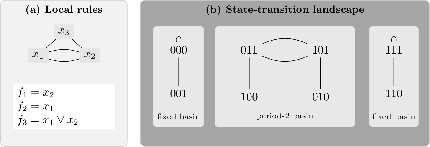
We study Boolean networks whose local functions are restricted to closed families of Boolean functions. These families classify local rules by their logical properties and provide a principled way to describe possible update mechanisms. The resulting problem is fixed-period and instance-level: given a network and a prescribed exact period \(k\), decide whether the attractor landscape contains a cyclic attractor of that period. Figure 1 illustrates these objects for a small network under parallel update; panel (b) is the full synchronous state-transition graph.
1.0.0.1 Contributions.
For every fixed \(k\ge 2\), we complete the Post-lattice classification of exact-period cyclic-attractor detection in this setting.
Every closed Boolean-function class gives either a polynomial-time problem or an \(\mathrm{NP}\)-complete problem.
The \(\mathrm{NP}\)-complete side begins as soon as the local rule class contains the majority-like monotone self-dual class or one of the two mixed conjunctive-disjunctive monotone classes.
All remaining Post classes fall into affine, purely conjunctive, or purely disjunctive regimes, where exact-period cyclic-attractor detection is decidable in polynomial time.
Together with the known fixed-point dichotomy for \(k=1\), this gives a complete Post-lattice classification of exact-period attractor detection at every fixed period.
Section 2 fixes the dynamical language of exact recurrence in Boolean networks. Section 3 turns the local-rule question into a Post-lattice dichotomy. Section 4 illustrates why cycles may occur on both sides of the boundary while being controlled by different mechanisms. Section 5 proves the boundary cases and lifts them to all Post classes. Section 6 discusses the dynamical meaning of the classification and its relation to complex-network attractor analysis. Section 7 concludes the article.
2 Boolean networks as finite nonlinear dynamical systems↩︎
To make the local-rule question precise, a Boolean network is treated throughout as a deterministic map on a finite state space. Its recurrent components are the attractors of the corresponding state-transition graph, and exact periods distinguish stationary recurrence from non-stationary cyclic behaviour.
For a positive integer \(n\), we write \[[n]=\{1,\ldots,n\}.\]
Let \(f_1,\ldots,f_n\) be Boolean functions \[f_i:\{0,1\}^n\to\{0,1\}, \qquad i\in[n].\]
Definition 1 (Boolean network and interaction digraph). A Boolean network on \(n\) components is a mapping \[f:\{0,1\}^n\to\{0,1\}^n, \qquad f=(f_1,\ldots,f_n),\] where each \(f_i\) is Boolean. The set \(\{0,1\}^n\) is the configuration space. Following [51], its interaction digraph is \(G_f=(V,E)\), where \(V=[n]\) and \(E\) is defined by \[(i,j)\in E \quad\Longleftrightarrow\quad f_j \text{ essentially depends on } x_i.\]
Let \(x\in\{0,1\}^n\) be a configuration and let \(I\subseteq[n]\). The partial update on \(I\) is the map \(f^{(I)}\) defined by \[f^{(I)}(x)_i= \begin{cases} f_i(x), & \text{if } i\in I,\\ x_i, & \text{if } i\notin I. \end{cases}\]
Definition 2 (Update schedule). Let \(W=(W_1,\ldots,W_t)\) be an ordered partition of \([n]\). The Boolean network with update schedule \(W\) is generated by \[f^{(W)}=f^{(W_t)}\circ\cdots\circ f^{(W_2)}\circ f^{(W_1)}.\] The case \(W=([n])\) gives \(f^{(W)}=f\) and is called the parallel, or synchronous, update scheme.
The update map \(f^{(W)}\) induces a directed state-transition graph whose vertices are the configurations in \(\{0,1\}^n\) and whose outgoing edge from \(x\) points to \(f^{(W)}(x)\). Since this graph is finite and deterministic, every trajectory eventually enters a directed cycle. These recurrent cycles are the attractors of the finite dynamical system.
Definition 3 (Attractors of exact period). A configuration \(x\in\{0,1\}^n\) has exact period \(k\) under \(f^{(W)}\) if \[\left(f^{(W)}\right)^k(x)=x\] and \[\left(f^{(W)}\right)^\ell(x)\neq x \qquad \text{for all } \ell\in\{1,\ldots,k-1\}.\] The corresponding orbit \[x,\;f^{(W)}(x),\;\ldots,\;\left(f^{(W)}\right)^{k-1}(x)\] is a cyclic attractor of exact period \(k\) when \(k\ge 2\). For \(k=1\), it is a fixed-point attractor. The set of configurations of exact period \(k\) is denoted by \[\Phi_k\left(f^{(W)}\right)= \left\{ x\in\{0,1\}^n \;\middle|\; \left(f^{(W)}\right)^k(x)=x \text{ and } \forall \ell\in\{1,\ldots,k-1\},\;\left(f^{(W)}\right)^\ell(x)\neq x \right\}.\] In the Boolean-network complexity literature, such cyclic attractors are often called limit cycles.
Local rule restrictions are expressed through closed classes of Boolean functions.
Definition 4 (Closure of a function class). Let \(\mathcal{F}\) be a set of Boolean functions. Its closure under superposition and introduction of fictitious variables is denoted by \([\mathcal{F}]\).
All complexity statements use a fixed finite basis, chosen before the input is given. Each coordinate function is represented by an acyclic circuit over this basis with inputs among \(x_1,\ldots,x_n\); repeated inputs are allowed, and constants are used when the class contains them. Since the basis is fixed and finite, gate fan-in is bounded by a constant. Circuit size counts gates and wires, including repeated input wires; if a constant belongs to the clone but not explicitly to the chosen basis, a fixed constant-size circuit for it is substituted. The instance size is \(n\) plus the total circuit size. For a closed Post class \(\mathcal{C}\), \(k\)-PLCE\((\mathcal{C})\) means this problem over any fixed finite basis of \(\mathcal{C}\). This is the standard circuit representation for finitely generated clones [58]. If two fixed finite bases generate the same clone, each gate of one basis has a constant-size circuit over the other. Replacing gates one by one therefore gives a linear-size translation between the corresponding circuit representations. Thus clone membership is a semantic condition on Boolean functions, while the reductions and algorithms below use only polynomial-time translations between these fixed representations.
With this notation, the decision problem is as follows. In each complexity statement, the period \(k\) is treated as a fixed parameter.
Problem 1 (\(k\)-PLCE\((\mathcal{F})\)). Fix an integer \(k\ge 1\) and a finite set \(\mathcal{F}\) of Boolean functions. The input is a Boolean network \(f=(f_1,\ldots,f_n)\) under the parallel update scheme, where each coordinate \(f_i\in[\mathcal{F}]\) is represented by a circuit over the fixed basis \(\mathcal{F}\). The question is whether \[\Phi_k(f)\neq\emptyset.\]
Dynamically, \(k\)-PLCE asks whether the attractor landscape contains a fixed point when \(k=1\), or a non-stationary recurrent pattern of prescribed exact period when \(k\ge 2\).
The hardness proofs use polynomial-time reductions from \(3\)-SAT, recalled here to keep the constructions self-contained.
Problem 2 (\(3\)-SAT). The input is a Boolean formula \(\psi\) in \(3\)-CNF on variables \(\{x_1,\ldots,x_n\}\). The question is whether there is an assignment \(a:\{x_1,\ldots,x_n\}\to\{0,1\}\) such that \(\psi(a)=1\).
Throughout the proofs, if \(z\in\{0,1\}^n\) is a configuration and \(v\in[n]\), then \(z_v\) denotes the value of coordinate \(v\) in \(z\). For a trajectory \(z^{(0)},z^{(1)},\ldots\) of the global update map, \(z_v^{(t)}\) denotes the value of coordinate \(v\) at time \(t\).
3 Local logical rule classes and main results↩︎
The local rule class is the modelling axis used in the classification. In complex-network language, this axis is distinct from topology or update schedule: two networks may have comparable interaction graphs, but their attractor landscapes can become easier or harder to analyse depending on whether the local rules are monotone, self-dual, linear, conjunctive, or disjunctive.
Following the notation of [59], the relevant closed classes of Boolean functions are as follows. The class \(D_2\) consists of monotone self-dual functions and is generated by the ternary majority function. More generally, for \(q\ge 0\) define the odd-arity majority function by \[\operatorname{maj}_{2q+1}(x_1,\ldots,x_{2q+1})=1 \quad\Longleftrightarrow\quad x_1+\cdots+x_{2q+1}\ge q+1.\] The sum is taken in \(\mathbb{Z}\). Thus \(\operatorname{maj}_3(x,y,z)=(x\wedge y)\vee(y\wedge z)\vee (x\wedge z)\). When the arity is clear from the list of arguments, we write \(\operatorname{maj}\); repeated arguments are allowed. The class \(F_6^\infty\), generated by \(x\wedge (y\vee z)\), consists of monotone functions that preserve both constants and are bounded above by one of their arguments; \(F_2^\infty\), generated by \(x\vee (y\wedge z)\), is the coordinatewise dual class. On the tractable side, \(L_1\) is the affine clone generated by \(\{1,x\oplus y\}\), while \(P_6=[\{x\wedge y,0,1\}]\) and \(S_6=[\{x\vee y,0,1\}]\) are the one-sided conjunctive and disjunctive clones with constants.
For the decision problem defined in Section 2, the classification is as follows.
Theorem 3 (Post-lattice dichotomy). Fix \(k\ge 2\). For every closed Boolean-function class \(\mathcal{C}\) in Post’s lattice, \(k\)-PLCE\((\mathcal{C})\) is either polynomial-time solvable or \(\mathrm{NP}\)-complete. More precisely, \(k\)-PLCE\((\mathcal{C})\) is \(\mathrm{NP}\)-complete if \(\mathcal{C}\) contains at least one of the classes \(D_2\), \(F_6^\infty\), or \(F_2^\infty\). In all remaining cases, \(\mathcal{C}\) is contained in \(L_1\), \(P_6\), or \(S_6\), and \(k\)-PLCE\((\mathcal{C})\) is decidable in polynomial time.
The relevant part of Post’s lattice explains why the six classes just listed exhaust all closed classes. Combined with the boundary lemmas in Section 5, this standard lattice separation turns the local results into a complete dichotomy. In the notation of [59], and as visualised in Figure 2, it can be stated as follows.
Lemma 1 (Post-lattice separation). Let \(\mathcal{C}\) be a closed class of Boolean functions. If \(\mathcal{C}\) contains none of \(D_2\), \(F_6^\infty\), and \(F_2^\infty\), then \[\mathcal{C}\subseteq L_1 \quad\mathrm{or}\quad \mathcal{C}\subseteq P_6 \quad\mathrm{or}\quad \mathcal{C}\subseteq S_6.\]
The stationary case \(k=1\) is exactly fixed-point existence, and Kosub’s fixed-point dichotomy for Post classes and minor-closed graph classes applies to the unrestricted interaction graph class [54]. Hence \(1\)-PLCE\((\mathcal{C})\) is \(\mathrm{NP}\)-complete precisely when \(\mathcal{C}\) contains the clone \(D_1\) of all self-dual functions, and is polynomial-time solvable otherwise.
The theorem shows that exact cyclic-attractor detection is not governed only by the size or topology of the network. The local logical mechanism matters: some highly restricted monotone rule families can still encode hard recurrent behaviour, whereas linearity and one-sided conjunctive/disjunctive structure provide enough algebraic order to make the same attractor question tractable.

4 Illustrative dynamical examples↩︎
The theorem separates mechanisms of recurrence, not the mere presence or absence of cycles. Non-stationary cyclic attractors occur on both sides of the dichotomy. The difference is that, in the tractable classes, the equations defining a prescribed period retain a rigid algebraic or order-theoretic form. In the hard classes, by contrast, a local rule can make the propagation of a periodic signal conditional on a Boolean consistency choice. The following small networks make this distinction visible at the level of trajectories.
4.0.0.1 Affine recurrence is algebraic.
Consider the \(L_1\)-network on two variables \[f(x_1,x_2)=\left(x_2,\;x_1\oplus x_2\right).\] For this network, \[f^2(x_1,x_2)=\left(x_1\oplus x_2,\;x_1\right), \qquad f^3(x_1,x_2)=\left(x_1,\;x_2\right).\] The configuration \(00\) is fixed, and the three non-zero configurations form the exact period-three attractor \[01\longmapsto 11\longmapsto 10\longmapsto 01.\] This example shows why the polynomial side of the dichotomy cannot be interpreted as a dynamical restriction to fixed points. Affine networks may have genuine non-stationary recurrence, but their recurrence equations remain linear: for an arbitrary affine network \(f(x)=Ax\oplus b\), the condition \(f^t(x)=x\) is a linear system over \(\mathbb{F}_2\) for every fixed \(t\). Exact period is obtained by removing solutions with smaller period, rather than by exploring the exponentially large state-transition graph.
4.0.0.2 One-sided recurrence is order-theoretic.
Now consider the \(P_6\)-network \[f(x_1,x_2,x_3)=\left(x_2,\;x_1,\;x_1\wedge x_2\right).\] It has the exact period-two orbit \[010\longmapsto 100\longmapsto 010,\] and the fixed points \(000\) and \(111\). In terms of zero sets \(Z(x)=\left\{i:x_i=0\right\}\), the two-cycle is \[\{1,3\}\longmapsto \{2,3\}\longmapsto \{1,3\}.\] The first two coordinates merely exchange their values, while the third coordinate remains zero because a conjunction is zero as soon as one of its inputs is zero. Thus the orbit is non-stationary, but it is governed by a closure rule for zero sets rather than by an arbitrary interaction among states. In a general conjunctive network, the condition \(f^t(x)=x\) can be read through how zeros propagate along the dependency graph over \(t\) steps. This is the order-theoretic reason why the \(P_6\) boundary leads to graph-reachability and strongly connected component conditions.
The disjunctive boundary is the same phenomenon under coordinatewise complementation. The dual \(S_6\)-network \[g(x_1,x_2,x_3)=\left(x_2,\;x_1,\;x_1\vee x_2\right)\] has the complementary exact period-two orbit \[101\longmapsto 011\longmapsto 101.\] In the dual view, sets of ones replace zero sets and satisfy the corresponding closure conditions. The two examples therefore represent the same tractable mechanism: cyclic behaviour is allowed, but the admissible cyclic patterns are controlled by monotone propagation in the dependency graph.
4.0.0.3 Hardness begins when signal transmission becomes conditional.
The hard side of the theorem relies on a different local mechanism. Let \[\operatorname{maj}(s,u,v)\] be the ternary majority function. It is monotone and self-dual, hence it belongs to the boundary class \(D_2\). With \(s\) viewed as a signal and \(u,v\) as auxiliary inputs, \[\operatorname{maj}(s,u,v)= \begin{cases} 0, & u=v=0,\\ s, & u\neq v,\\ 1, & u=v=1. \end{cases}\] The same local rule therefore has two distinct modes. If the auxiliary inputs are equal, the output is forced to a constant; if they are different, the signal passes through unchanged.
This distinction can already be seen in a two-coordinate cycle module with auxiliary coordinates that remain fixed along the trajectory. Set \[h_1(c_1,c_2)=\operatorname{maj}(c_2,u,v), \qquad h_2(c_1,c_2)=c_1.\] When \(u\neq v\), the map on \((c_1,c_2)\) is \((c_1,c_2)\mapsto(c_2,c_1)\), so \(10\) and \(01\) form an exact period-two attractor. When \(u=v=0\) or \(u=v=1\), one coordinate is forced, and the non-stationary cycle disappears. Thus the existence of a periodic orbit can depend on whether an auxiliary layer can realise the balanced condition.
On the hard side of the dichotomy, this phenomenon is amplified. The periodic layer can remain simple: it is a shift of a prescribed pattern. The nontrivial part is the auxiliary layer, whose local tests encode the consistency of a Boolean assignment. A cyclic attractor exists only when those tests place the pivotal gate in its transmitting mode. This explains the hard side of the main dichotomy without changing the nature of the desired attractor: the cycle remains a finite recurrent orbit, but its existence becomes tied to a global satisfiability constraint. The same mechanisms reappear in the boundary proofs: linear recurrence in Lemma 6, zero- or one-set closure in Lemmas 7 and 8, and conditional transmission in Lemma 3.
5 Proofs↩︎
The proof of Theorem 3 has four steps. First, Lemma 2 records that inclusion of local rule classes gives polynomial-time reductions. Second, Lemmas 3, 4, and 5 prove \(\mathrm{NP}\)-completeness for the three hard boundary classes \(D_2\), \(F_6^\infty\), and \(F_2^\infty\); by monotonicity, every closed class containing one of them is hard. Third, Lemmas 6, 7, and 8 give polynomial-time algorithms for the three tractable boundary classes \(L_1\), \(P_6\), and \(S_6\); hence all their subclasses are tractable. Finally, Lemma 1 shows that every closed class containing none of the hard boundaries is contained in one of these tractable boundaries.
Throughout this section \(k\ge 2\) is fixed. The first observation is monotonicity with respect to the local rule class. We write \(\le_{\mathrm{P}}\) for polynomial-time many-one reducibility [60].
Lemma 2. Let \(\mathcal{F}_1\) and \(\mathcal{F}_2\) be sets of Boolean functions such that \(\mathcal{F}_1 \subseteq \mathcal{F}_2\). Then \[\mathrm{k-PLCE}(\mathcal{F}_1) \le_{\mathrm{P}} \mathrm{k-PLCE}(\mathcal{F}_2).\]
Proof of Lemma 2. The inclusion \(\mathcal{F}_1\subseteq\mathcal{F}_2\) implies \([\mathcal{F}_1]\subseteq[\mathcal{F}_2]\), because both closures are formed by the same closure operations: superposition and introduction of fictitious variables. Thus every instance \(f=(f_1,\ldots,f_n)\) of \(k\)-PLCE\((\mathcal{F}_1)\) is already an instance of \(k\)-PLCE\((\mathcal{F}_2)\). The identity map on instances is computable in linear time and preserves the answer, since it asks about the same global Boolean network, yielding the required many-one reduction. ◻
The first hardness boundary is the monotone self-dual class \(D_2\).
Lemma 3. For every fixed integer \(k\ge 2\), \(\mathrm{k-PLCE}(D_2)\) is \(\mathrm{NP}\)-complete.
Proof of Lemma 3. Membership in \(\mathrm{NP}\) follows because \(k\) is fixed: a certificate is a configuration \(x\), and one verifies \(f^k(x)=x\) and \(f^\ell(x)\neq x\) for all \(\ell<k\) by computing the first \(k\) iterates. For \(\mathrm{NP}\)-hardness we reduce from \(3\)-SAT. Let \(\psi=C_1\wedge\cdots\wedge C_m\) be a \(3\)-CNF formula over variables \(y_1,\ldots,y_n\), with \(C_j=(\ell_{j1}\vee\ell_{j2}\vee\ell_{j3})\). By adding at most \(n\) copies of one clause, without changing satisfiability, we may assume that \(\gcd(n,m)=1\).
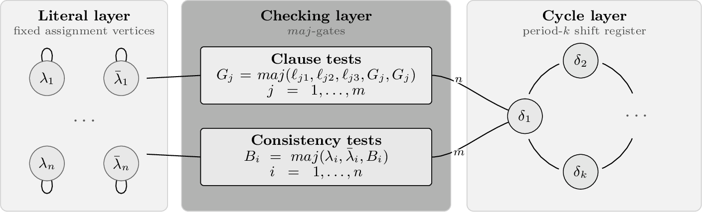
We build a network \(\mathcal{N}_\psi\) in three layers. The literal layer has two fixed vertices \(\lambda_i,\bar\lambda_i\) for each variable \(y_i\), with local functions \(f_{\lambda_i}(z)=z_{\lambda_i}\) and \(f_{\bar\lambda_i}(z)=z_{\bar\lambda_i}\). The checking layer has clause vertices \(G_j\) and consistency vertices \(B_i\). The vertex \(G_j\) receives the three literal inputs corresponding to \(C_j\) and two self-loops; the vertex \(B_i\) receives \(\lambda_i,\bar\lambda_i\) and one self-loop. Each of these vertices applies the appropriate odd-arity instance of \(\operatorname{maj}\), which is monotone and self-dual and hence belongs to \(D_2\).
The cycle layer consists of vertices \(\delta_1,\ldots,\delta_k\). For \(r=2,\ldots,k\), set \(f_{\delta_r}(z)=z_{\delta_{r-1}}\). The vertex \(\delta_1\) applies \(\operatorname{maj}\) to the value of \(\delta_k\), to \(n\) copies of each \(G_j\), and to \(m\) copies of each \(B_i\). Thus every local function of \(\mathcal{N}_\psi\) lies in \(D_2\), and the construction is polynomial-time.
Figure 3 summarizes the role of the three layers in the reduction.
Assume first that \(\psi\) is satisfied by an assignment \(a\). Put \(z_{\lambda_i}^{(0)}=a(y_i)\), \(z_{\bar\lambda_i}^{(0)}=1-a(y_i)\), \(z_{G_j}^{(0)}=1\), \(z_{B_i}^{(0)}=0\), and \(\left(z_{\delta_1}^{(0)},\ldots,z_{\delta_k}^{(0)}\right) =\left(1,0,\ldots,0\right)\). The literal values are fixed. Since each clause contains a true literal, every \(G_j\) sees at least one true literal and two loop inputs equal to \(1\), so it remains equal to \(1\). Each \(B_i\) sees exactly one of \(\lambda_i,\bar\lambda_i\) equal to \(1\) and its own value equal to \(0\), so it remains equal to \(0\). Hence the checking layer is fixed. At \(\delta_1\), the checking-layer inputs contribute \(mn\) ones and \(mn\) zeros, so the update at \(\delta_1\) is determined by the remaining input \(\delta_k\). Together with \(f_{\delta_r}=z_{\delta_{r-1}}\) for \(r\ge 2\), the cycle layer performs a cyclic shift of \(\left(1,0,\ldots,0\right)\). Therefore the constructed network has a cyclic attractor of exact period \(k\).
Conversely, suppose that \(z^{(0)}\in\Phi_k(f)\) for the constructed network. The literal vertices are constant. With literal inputs fixed, each \(G_j\) and \(B_i\) evolves by a monotone map \(T:\{0,1\}\to\{0,1\}\) of its own current value. On this two-point state space, any nonconstant periodic orbit would be a two-cycle; monotonicity excludes this, because \(T(0)=1\) and \(T(1)=0\) would be required. Hence these vertices are constant on the periodic trajectory. Let \(p=\#\left\{j:z_{G_j}=1\right\}\) and \(q=\#\left\{i:z_{B_i}=1\right\}\). If \(\delta_1\) were constant, then all \(\delta\)-vertices would be constant, contradicting exact period \(k\ge 2\). Thus the update at \(\delta_1\) must depend on the input from \(\delta_k\), which is possible only when the other inputs are balanced: \(pn+qm=mn\). Reducing modulo \(n\) gives \(qm\equiv 0\pmod n\), and reducing modulo \(m\) gives \(pn\equiv 0\pmod m\). Since \(\gcd(n,m)=1\), we have \(n\mid q\) and \(m\mid p\). Together with \(0\le q\le n\) and \(0\le p\le m\), this gives \(q\in\{0,n\}\), \(p\in\{0,m\}\), and hence either \((p,q)=(m,0)\) or \((p,q)=(0,n)\).
If \((p,q)=(m,0)\), define \(a(y_i)=z_{\lambda_i}\). For any clause \(C_j\), the vertex \(G_j\) has value \(1\), and its two loop inputs are equal to \(1\); therefore at least one literal input of \(G_j\) is \(1\). If that input is \(\lambda_i\), then \(y_i\) is true under \(a\). If it is \(\bar\lambda_i\), then \(z_{\lambda_i}\) cannot also be \(1\), since \(B_i=0\) and \(B_i\) computes \(\operatorname{maj}(\lambda_i,\bar\lambda_i,B_i)\). Hence \(z_{\lambda_i}=0\), and \(\neg y_i\) is true under \(a\).
If \((p,q)=(0,n)\), define \(a(y_i)=1-z_{\lambda_i}\). Now every \(G_j\) has value \(0\), with two loop inputs equal to \(0\), so at least one literal input of \(G_j\) is \(0\). If that input is \(\lambda_i\), then \(y_i\) is true under \(a\). If it is \(\bar\lambda_i\), then \(z_{\lambda_i}=1\); otherwise \(\operatorname{maj}(\lambda_i,\bar\lambda_i,B_i)\) would be \(0\), contradicting \(B_i=1\). Thus \(\neg y_i\) is true under \(a\). In both cases every clause of \(\psi\) is satisfied. The reduction is correct, so \(k\)-PLCE\((D_2)\) is \(\mathrm{NP}\)-hard; together with membership in \(\mathrm{NP}\), it is \(\mathrm{NP}\)-complete. ◻
Lemma 4. For every fixed integer \(k\ge 2\), \(\mathrm{k-PLCE}(F_{6}^{\infty})\) is \(\mathrm{NP}\)-complete.
Proof of Lemma 4. Membership in \(\mathrm{NP}\) follows because \(k\) is fixed and a candidate configuration can be verified by computing its first \(k\) iterates. For hardness we reduce from \(k\)-PLCE\((D_2)\). Given a \(D_2\)-network \(f=(f_1,\ldots,f_n)\), add a control coordinate \(y\) and define a network \(g=(g_0,g_1,\ldots,g_n)\) by \[g_0(y,x)=y,\qquad g_i(y,x)=y\wedge f_i(x),\quad i\in[n].\] We use the standard Post-lattice description of \(F_6^\infty\): a Boolean function belongs to this class exactly when it is monotone, preserves \(0\) and \(1\), and is bounded above by one of its variables [58], [59]. The function \(g_0\) has these properties. For \(i\ge 1\), the function \(f_i\in D_2\) is monotone and self-dual; hence monotonicity and self-duality force \(f_i(0,\ldots,0)=0\) and \(f_i(1,\ldots,1)=1\). Therefore \(g_i=y\wedge f_i\) is monotone, preserves both constants, and satisfies \(g_i(y,x)\le y\). Thus all coordinates of \(g\) lie in \(F_6^\infty\). The fixed-basis representation is handled by a local circuit substitution. For every arity-\(r\) gate \(b\) of the fixed \(D_2\)-basis, define \[\widehat b(y,u_1,\ldots,u_r)=y\wedge b(u_1,\ldots,u_r).\] Both \(\widehat b\) and \((y,u)\mapsto y\wedge u\) lie in \(F_6^\infty\): they are monotone, preserve \(0\) and \(1\), and are bounded above by \(y\). Hence they have constant-size circuits over the fixed \(F_6^\infty\)-basis, so the output is an ordinary circuit over that basis. Leave the input variables unchanged, replace every \(D_2\)-gate \(b\) by the circuit for \(\widehat b\) with the same input \(y\), and add one final \((y,u)\mapsto y\wedge u\) gate at the output. The transformed circuit then computes \(y\wedge f_i(x)\), with only linear growth in size.
If \(x^{(0)}\in\Phi_k(f)\), then \(z^{(0)}=\left(1,x^{(0)}\right)\) lies in \(\Phi_k(g)\): the control coordinate remains equal to \(1\), and the remaining coordinates follow exactly the trajectory of \(f\). Conversely, let \(z^{(0)}=\left(y^{(0)},x^{(0)}\right)\in\Phi_k(g)\). Since \(g_0(y,x)=y\), the control coordinate is constant. If \(y^{(0)}=0\), all original coordinates become \(0\) after one step, so no cycle of exact period \(k\ge 2\) is possible. Hence \(y^{(0)}=1\), and then the \(x\)-coordinates satisfy \(x^{(t+1)}=f\left(x^{(t)}\right)\). Exact period \(k\) for \(z^{(0)}\) therefore implies exact period \(k\) for \(x^{(0)}\) under \(f\).
The construction is polynomial-time and preserves positive instances in both directions. Since \(k\)-PLCE\((D_2)\) is \(\mathrm{NP}\)-complete by Lemma 3, \(k\)-PLCE\((F_6^\infty)\) is \(\mathrm{NP}\)-complete. ◻
The dual monotone boundary is obtained by coordinatewise complementation.
Lemma 5. For every fixed integer \(k\ge 2\), \(\mathrm{k-PLCE}(F_{2}^{\infty})\) is \(\mathrm{NP}\)-complete.
Proof of Lemma 5. Membership in \(\mathrm{NP}\) follows from the same fixed-period verification. The same Post-lattice description identifies \(F_{2}^{\infty}\) as the coordinatewise dual of \(F_{6}^{\infty}\): if \(h\in F_6^\infty\), then \(h^\ast(x)=\neg h(\neg x_1,\ldots,\neg x_n)\) belongs to \(F_2^\infty\), and conversely [59]. Given an \(F_6^\infty\)-network \(f\), define the coordinatewise dual network \[g_i(x)=\neg f_i(\neg x_1,\ldots,\neg x_n),\qquad i\in[n].\] Then \(g\) is an \(F_2^\infty\)-network and the complement map \(c(x)=\neg x\) satisfies \(g(c(x))=c(f(x))\). Hence \(x\in\Phi_k(f)\) if and only if \(c(x)\in\Phi_k(g)\). The polynomial-time transformation and Lemma 4 show that \(\mathrm{k-PLCE}(F_{2}^{\infty})\) is \(\mathrm{NP}\)-complete. ◻
For the affine boundary \(L_1\), exact-period existence is reducible to linear algebra. The resulting algorithm runs in time \(O\left(n^3k\right)\) by counting configurations whose periods divide \(k\).
Lemma 6. For every fixed integer \(k\ge 2\), \(\mathrm{k-PLCE}(L_1)\in \mathrm{P}\).
Proof of Lemma 6. Let \(f=(f_1,\ldots,f_n)\) be an \(L_1\)-network. Its global map is affine over \(\mathbb{F}_2\). From the input circuits, the affine representation of each coordinate is computed bottom-up: each gate contributes the xor of the coefficient vectors of its inputs, and the constant gate contributes the constant term. Thus in polynomial time we obtain \(f(x)=Ax\oplus b\), with \(A\in\mathbb{F}_2^{n\times n}\) and \(b\in\mathbb{F}_2^n\). For \(t\ge 1\), let \(S(t)=\left|\left\{x\in\mathbb{F}_2^n:f^t(x)=x\right\}\right|\), and let \(P(d)\) be the number of configurations of minimal period \(d\). Since a point is fixed by \(f^t\) exactly when its minimal period divides \(t\), \(S(t)=\sum_{d\mid t}P(d)\). Möbius inversion gives \(P(k)=\sum_{d\mid k}\mu\left(k/d\right)S(d)\), where \(\mu\) is the Möbius function. Thus the problem reduces to computing \(S(d)\) for all divisors \(d\mid k\) and testing whether \(P(k)>0\).
Introduce the standard affine lift \[M= \begin{pmatrix} A & b\\ 0 & 1 \end{pmatrix} \in \mathbb{F}_2^{(n+1)\times(n+1)}.\] By induction, \(M^t\) has the form \[M^t= \begin{pmatrix} A_t & b_t\\ 0 & 1 \end{pmatrix}, \qquad\text{with}\qquad f^t(x)=A_t x\oplus b_t.\] For each divisor \(d\mid k\), the equation \(f^d(x)=x\) is therefore the linear system \((A_d\oplus I)x=b_d\) over \(\mathbb{F}_2\). Gaussian elimination gives the number \(S(d)\) of its solutions in \(O\left(n^3\right)\) time. The matrices \(M,\ldots,M^k\) are obtained sequentially in \(O\left(n^3k\right)\) time, and there are at most \(k\) relevant divisors. Computing \(P(k)\) from the Möbius formula then adds only \(O\left(k\right)\) arithmetic operations. Hence existence of a cyclic attractor of exact period \(k\) is decidable in \(O\left(n^3k\right)\) time after the polynomial-time conversion to the \(n\)-dimensional affine representation. Since \(k\) is fixed in the decision problem, this is polynomial in the input size, and the problem belongs to \(\mathrm{P}\). ◻
For conjunctive local rules with constants, zero sets provide the relevant combinatorial representation under iterates of the network.
Lemma 7. For every fixed integer \(k\ge 2\), \(\mathrm{k-PLCE}(P_6)\in \mathrm{P}\).
Proof of Lemma 7. Recall that every \(P_6\)-function is either \(0\), \(1\), or a conjunction of variables. Since the basis is fixed, each coordinate circuit is normalised to this form in polynomial time by a bottom-up pass: each basis gate has a precomputed \(0\), \(1\), or conjunction-of-selected-arguments description, and applying it to already normalised inputs only propagates constants and takes unions of input sets. If the \(v\)-th coordinate is not identically \(0\), write \(\operatorname{In}(v)\) for its input set and \[f_v(x)=\bigwedge_{u\in \operatorname{In}(v)}x_u,\] with the empty conjunction interpreted as \(1\). We compute the same representation for \(f_v^t\), \(1\le t\le k\): either \(f_v^t\equiv0\), or \(f_v^t(x)=\bigwedge_{u\in \operatorname{In}_t(v)}x_u\). The induction step substitutes the already computed representations of the coordinates in \(\operatorname{In}(v)\). If one substituted coordinate is identically \(0\), then \(f_v^{t+1}\equiv0\); otherwise \[\operatorname{In}_{t+1}(v)= \bigcup_{w\in \operatorname{In}(v)}\operatorname{In}_t(w).\] Since \(k\) is fixed, this takes polynomial time. Let \(H_t=([n],E_t)\) be the dependency graph of \(f^t\), with \((u,v)\in E_t\) iff \(u\in \operatorname{In}_t(v)\); if \(f_v^t\equiv0\), no edge is put into \(v\).
For conjunctive maps, fixed-point conditions are naturally expressed through the zero set \(Z=\{v:x_v=0\}\). Let \(C_0^k=\{v:f_v^k\equiv0\}\) be the coordinates forced to zero by the \(k\)-th iterate. Then \(f^k(x)=x\) if and only if \[C_0^k\subseteq Z,\qquad Z \text{ is successor-closed in } H_k,\qquad \operatorname{In}_k(v)\cap Z\neq\emptyset \text{ for every }v\in Z\setminus C_0^k .\] Here successor-closed means that every out-neighbour in \(H_k\) of a vertex in \(Z\) also belongs to \(Z\). Indeed, a coordinate equal to \(1\) remains \(1\) exactly when none of its inputs in \(H_k\) is zero, while a nonconstant coordinate equal to \(0\) remains \(0\) exactly when at least one input is zero.
This criterion gives \(f^k(x)=x\); exact period \(k\) additionally requires a mismatch \(f^\ell(x)\neq x\) for every \(\ell<k\). We encode one such mismatch by a pair \((P,Q)\) of vertex sets: a zero set \(Z\) realises \((P,Q)\) if \(P\subseteq Z\) and \(Q\cap Z=\emptyset\). For a fixed \(\ell\), the list \(A_\ell\) consists of the following local witnesses, over all coordinates \(v\): \[(\emptyset,\{v\}) \quad\text{if } f_v^\ell\equiv0,\] \[(\{u\},\{v\}) \quad\text{for each }u\in \operatorname{In}_\ell(v) \quad\text{if } f_v^\ell\not\equiv0,\] and \[(\{v\},\operatorname{In}_\ell(v)) \quad\text{if } f_v^\ell\not\equiv0.\] These three types are exhaustive. An identically zero coordinate function can disagree with \(x_v\) only when \(x_v=1\). A conjunction disagrees either because \(x_v=1\) while some input \(u\) is zero, or because \(x_v=0\) while all its inputs are \(1\). Thus, for the configuration with zero set \(Z\), realising some witness in \(A_\ell\) is equivalent to \(f^\ell(x)\neq x\). For instance, when \(k=2\) and \(f_v=x_a\wedge x_b\), the witnesses attached to \(v\) are \((\{a\},\{v\})\), \((\{b\},\{v\})\), and \((\{v\},\{a,b\})\). Each coordinate contributes at most \(\left|\operatorname{In}_\ell(v)\right|+2\le n+2\) witnesses, so \(|A_\ell|=O(n^2)\).
We now combine the inequalities \(f^\ell(x)\neq x\), \(\ell<k\), with the fixed-point criterion for \(f^k\). The algorithm considers all choices of witnesses, one pair \((P_\ell,Q_\ell)\in A_\ell\) for each \(\ell=1,\ldots,k-1\). For such a choice, put \[P=C_0^k\cup\bigcup_{\ell=1}^{k-1}P_\ell, \qquad Q=\bigcup_{\ell=1}^{k-1}Q_\ell .\] Call this witness choice feasible if \(P\cap Q=\emptyset\) and there exists a zero set \(Z\) such that \(P\subseteq Z\), \(Z\cap Q=\emptyset\), and \(Z\) satisfies the fixed-point criterion. Thus a feasible choice is precisely one whose selected witnesses can be realised by a configuration satisfying \(f^k(x)=x\).
It remains to test feasibility under the assumption \(P\cap Q=\emptyset\). Define \[S=\left\{v\in[n]\;\middle|\; \text{no vertex of }Q\text{ is reachable from }v\text{ in }H_k\right\}.\] Reachability includes paths of length \(0\). Then \(S\) is the largest successor-closed set disjoint from \(Q\). Hence every zero set satisfying the feasibility conditions is contained in \(S\); if \(P\not\subseteq S\), no such zero set exists. Assume from now on that \(P\subseteq S\).
Write \(H_k[S]\) for the subgraph of \(H_k\) induced by \(S\). In \(H_k[S]\), call a strongly connected component cyclic if it has more than one vertex or has a loop. Let \(B\) be the union of \(C_0^k\) and all cyclic strongly connected components of \(H_k[S]\), and let \(C\) be the set of vertices reachable from \(B\) inside \(H_k[S]\). We claim that the witness choice is feasible if and only if \(P\subseteq C\).
For necessity, let \(Z\subseteq S\) satisfy the feasibility conditions. Vertices in \(Z\cap C_0^k\) already lie in \(B\subseteq C\). Now take \(v\in Z\setminus C_0^k\). By the predecessor condition in the fixed-point criterion, there is an edge \(u\to v\) in \(H_k\) with \(u\in Z\). Repeating this step inside the finite set \(Z\) either reaches \(C_0^k\) or repeats a vertex. In the first case, the resulting path runs forward from \(C_0^k\subseteq B\) to \(v\). In the second, the repeated segment is a directed cycle in \(H_k[S]\), hence lies in a cyclic component included in \(B\), and the remaining path again runs forward to \(v\). Thus every zero set satisfying the feasibility conditions is contained in \(C\), so \(P\subseteq C\) is necessary.
Conversely, if \(P\subseteq C\), then \(C\) itself satisfies the feasibility conditions. It is successor-closed because \(S\) is successor-closed and every successor of a vertex reachable from \(B\) is again reachable from \(B\). Moreover, every vertex of \(C\setminus C_0^k\) has a predecessor in \(C\): inside a cyclic component this predecessor lies in the component, and outside it is the previous vertex on a path from \(B\). Since \(C\subseteq S\), it is disjoint from \(Q\), and \(P\subseteq C\) holds by assumption. Thus \(C\) satisfies the fixed-point criterion and realises the selected witnesses.
If a feasible witness choice exists, the configuration whose zero set is the corresponding \(C\) satisfies \(f^k(x)=x\) and realises one witness for every \(\ell<k\); hence \(x\in\Phi_k(f)\). Conversely, any \(x\in\Phi_k(f)\) determines, for each \(\ell<k\), one of these witnesses from a coordinate where \(f^\ell(x)\neq x\). Its zero set satisfies the fixed-point criterion, so these selected witnesses form a feasible witness choice.
There are at most \(O(n^{2(k-1)})\) witness choices, and \(k\) is fixed. For each choice, reachability, strongly connected components, and set inclusions are computed in polynomial time. Therefore \(k\)-PLCE\((P_6)\in \mathrm{P}\). ◻
Boolean duality reduces the disjunctive case to the conjunctive one, with zeros and ones interchanged.
Lemma 8. For every fixed integer \(k\ge 2\), \(\mathrm{k-PLCE}(S_6)\in \mathrm{P}\).
Proof of Lemma 8. Recall that \(P_6=[\{x\wedge y,0,1\}]\) and \(S_6=[\{x\vee y,0,1\}]\). Given an \(S_6\)-network \(f=(f_1,\ldots,f_n)\), define the coordinatewise dual network \[g_i(x_1,\ldots,x_n) = \neg f_i(\neg x_1,\ldots,\neg x_n), \qquad i\in[n].\] By De Morgan’s law, disjunctions become conjunctions and the constants \(0\) and \(1\) are interchanged, so \(g\) is a \(P_6\)-network and is computable from \(f\) in polynomial time.
Let \(c(x_1,\ldots,x_n)=(\neg x_1,\ldots,\neg x_n)\). By construction, \(g(c(x))=c(f(x))\), so \(g\circ c=c\circ f\). Induction gives \(g^t(c(x))=c(f^t(x))\) for every \(t\ge1\). Hence \(x\in\Phi_k(f)\) if and only if \(c(x)\in\Phi_k(g)\), and therefore \(\Phi_k(f)\neq\emptyset\) iff \(\Phi_k(g)\neq\emptyset\). The reduction to \(k\)-PLCE\((P_6)\) is polynomial-time, and Lemma 7 completes the proof. ◻
Proof of Theorem 3. Let \(\mathcal{C}\) be a closed Boolean-function class in Post’s lattice. If \(\mathcal{C}\) contains \(D_2\), \(F_6^\infty\), or \(F_2^\infty\), then the corresponding boundary lemma and Lemma 2 give \(\mathrm{NP}\)-hardness. Membership in \(\mathrm{NP}\) follows because \(k\) is fixed and a candidate configuration can be verified by computing its first \(k\) iterates. Therefore \(k\)-PLCE\((\mathcal{C})\) is \(\mathrm{NP}\)-complete.
If \(\mathcal{C}\) contains none of \(D_2\), \(F_6^\infty\), and \(F_2^\infty\), then Lemma 1 places \(\mathcal{C}\) inside one of the tractable boundary classes \(L_1\), \(P_6\), or \(S_6\). The corresponding polynomial-time boundary algorithm applies to all instances over \(\mathcal{C}\). Thus \(k\)-PLCE\((\mathcal{C})\) is polynomial-time solvable. The dichotomy follows. ◻
6 Discussion↩︎
Within the fixed-period setting considered here, the dichotomy isolates a local source of complexity in finite nonlinear network dynamics. Studies of complex networks often vary topology, coupling, delays, or update protocols to understand global behaviour [1], [2]. In the present classification, the interaction graph is unrestricted, but the admissible Boolean operations at the nodes are varied. The local rule class can therefore determine whether exact cyclic-attractor existence for the prescribed period is decidable in polynomial time or encodes an \(\mathrm{NP}\)-complete search problem.
The classification also complements the probabilistic theory of Boolean networks. Random Boolean-network models relate order, criticality, sensitivity, and attractor statistics to connectivity, bias, and rule distributions [25], [27]. Damage-spreading analyses and studies of regulatory logic classes further show that these local choices affect dynamical regimes in Boolean and cellular-automaton models [32], [33]. The dichotomy addresses the instance-level counterpart. For a fixed finite network and a fixed prescribed period, it identifies which local rule classes make cyclic-attractor existence algorithmically accessible.
This worst-case boundary complements practical attractor-analysis methods rather than replacing them. Some recent tools use a priori information or symbolic bifurcation analysis [44], [45]; others exploit trap-space structure and network reduction to identify attractors in large biological models [61], [62]. Software tools such as BooN provide another implementation-oriented layer for Boolean-network analysis [46]. Answer Set Programming provides a complementary way to encode Boolean-network dynamics and enumerate stable or cyclic attractors in biological models [42]. These methods exploit additional structure present in concrete networks. The dichotomy identifies which local rule families can still contain worst-case hard instances even when the period is fixed, and which families impose enough algebraic or order structure to avoid that hardness.
The \(\mathrm{NP}\)-complete side shows that strong local restrictions do not by themselves rule out hard recurrent behaviour. Monotone self-dual rules and the two one-sided monotone boundary classes can still transmit enough information to encode satisfiability. This extends the complexity picture for limit-cycle problems and fixed-point dichotomies in Boolean dynamical systems [51], [54]: the passage from \(k=1\) to a fixed \(k\ge 2\) changes the boundary classes, but still admits a complete Post-lattice description.
The polynomial cases reveal the mechanisms that prevent such encodings. In the affine case, exact-period existence reduces to linear algebra over \(\mathbb{F}_2\). In the conjunctive and disjunctive cases with constants, the relevant constraints are captured by closure properties of zero sets or one sets in dependency graphs. Thus tractability is not a consequence of monotonicity alone; it depends on the particular algebraic or order structure carried by the local rule class.
For modelling applications, the dichotomy gives an algorithmic interpretation of modelling assumptions. Boolean networks model regulatory systems [6], [7], neural computation [9], and social dynamics [13]; local rule restrictions may encode activation, inhibition, or interpretability assumptions. Work on controllability asks how interventions can steer biological Boolean networks toward selected original attractors [63]. A recent analysis relates difficult control to instability in biologically inspired Boolean networks [64]. Related lattice-based descriptions connect regulatory rule structure with global dynamics [65]. These assumptions can therefore affect both observable attractor landscapes and worst-case detection complexity.
The results are specific to parallel update and to exact periods prescribed in advance. Under asynchronous semantics, attractors are usually defined as recurrent components of a transition graph rather than as single periodic orbits. Signed-cycle structure and network reduction then play different roles [24], [61], and motif constraints provide another source of restrictions on asynchronous attractors [66]. The dichotomy therefore provides a baseline for the parallel-update case rather than a direct classification of asynchronous Boolean dynamics.
7 Conclusions↩︎
We have proved a complete Post-lattice dichotomy for the exact-period cyclic-attractor problem in the parallel-update model with fixed-basis circuit inputs defined in Section 2. For every fixed \(k\ge 2\), the problem is \(\mathrm{NP}\)-complete for every Post class containing \(D_2\), \(F_6^\infty\), or \(F_2^\infty\). All remaining Post classes are covered by the polynomial-time boundary represented by \(L_1\), \(P_6\), and \(S_6\). Together with the known fixed-point classification for \(k=1\), this completes the prescribed-period existence classification over Post’s lattice for every fixed period.
Consequently, in this fixed-period setting, exact cyclic recurrence is controlled not only by the interaction graph, but also by the algebraic and order-theoretic properties of the local update rules. Some rule classes impose enough linear or closure structure to make exact-period detection tractable; others, despite strong local restrictions, can encode hard global constraints. This separates two notions that are often conflated in finite nonlinear models: local regularity of the update rule and computational accessibility of the recurrent dynamics.
Several directions remain open. These include the case in which the period is part of the input, restrictions on the interaction graph by degree or feedback structure, and asynchronous, sequential, or block-sequential update schemes. A further direction is to compare these exact worst-case boundaries with the attractor statistics observed in random and application-driven Boolean networks. Such comparisons would connect this classification with the broader question of how local logical constraints shape observable recurrent behaviour in complex discrete dynamical systems.
Acknowledgements↩︎
This work was supported by the Ministry of Economic Development of the Russian Federation in accordance with the subsidy agreement (agreement identifier 000000C313925P4H0002; grant No. 139-15-2025-012).
Data availability↩︎
No datasets were generated or analysed during the current study.